a condition-based maintenance policy and input parameters ... · fessors benjamim r. menezes and...
TRANSCRIPT

MAXSTALEY LENINYURI NEVES
A Condition-Based Maintenance
Policy and Input Parameters
Estimation for Deteriorating Systems
under Periodic Inspection
Belo Horizonte, MG, Brasil
Marco 2010
Universidade Federal de Minas Gerais
Escola de Engenharia
Programa de Pos-Graduacao em Engenharia Eletrica
A Condition-Based Maintenance
Policy and Input Parameters
Estimation for Deteriorating Systems
under Periodic InspectionMaxstaley Leninyuri Neves
Dissertacao de mestrado submetida
ao Programa de Pos-Graduacao em
Engenharia Eletrica da Universidade
Federal de Minas Gerais, como requi-
sito parcial a obtencao do Tıtulo de
Mestre em Engenharia Eletrica.
Area de Concentracao: Engenharia de
Computacao e Telecomunicacoes
Linha de Pesquisa: Sistemas de Com-
putacao
Orientador: Prof. Dr. Carlos A. Maia
Co-Orientador: Prof. Dr. Leonardo P. Santiago
Belo Horizonte, MG, Brasil
Marco 2010

i

Acknowledgments
I would like to acknowledge my supervisors, Professors Carlos A. Maia and
Leonardo P. Santiago, who each in their way supported me in this work. I am
greatly thankful for their guidance and support. I am also thankful to Pro-
fessors Benjamim R. Menezes and Marta A. Freitas, dissertation committee
members, for the careful review and extremely useful feedback.
This research was partially supported by the Laboratorio de Apoio a
Decisao e Confiabilidade whose people deserve thanks for many discussions
and insights, as well as my colleagues at the Programa de Pos-Graduacao em
Engenharia Eletrica and at the Programa de Pos-Graduacao em Engenharia
de Producao.
Throughout my years at Universidade Federal de Minas Gerais I have had
the opportunity to interact with several people who influenced my education.
I would like to thank all them, specially my former T.A. and R.A. supervisors
and my former teachers.
ii

Agradecimentos
Eu gostaria de agradecer aos meus orientadores, Professores Carlos A. Maia
e Leonardo P. Santiago, pelo apoio que me foi oferecido, cada um a sua
maneira. Sou muito grato pela orientacao e suporte. Agradeco tambem aos
Professores Benjamim R. Menezes e Marta A. Freitas, membros da banca,
pela cuidadosa revisao do texto e pelos importantes comentarios.
Esta pesquisa contou parcialmente com o apoio do Laboratorio de Apoio a
Decisao e Confiabilidade, cujas pessoas merecem meus agradecimentos pelas
varias discussoes e “insights”, da mesma maneira que meus colegas do Pro-
grama de Pos-Graduacao em Engenharia Eletrica e do Programa de Pos-
Graduacao em Engenharia de Producao.
Durante meus anos na Universidade Federal de Minas Gerais eu tive a
oportunidade de interagir com varias pessoas que influenciaram minha edu-
cacao. Eu gostaria de agradecer a todo(a)s, especialmente aos meus ex-
orientadores de pesquisa/monitoria e ex-professores.
iii
Abstract
We study the problem of proposing Condition-Based Maintenance policies for
machines and equipments. Our approach combines an optimization model
and input parameters estimation from empirical data.
The system deterioration is described by discrete states ordered from the
state “as good as new” to the state “completely failed”. At each periodic
inspection, whose outcome might not be accurate, a decision has to be made
between continuing to operate the system or stopping and performing its
preventive maintenance. This decision-making problem is discussed and we
tackle it by using an optimization model based on the Dynamic Programming
and Optimal Control theory.
We then explore the problem of how to estimate the model input param-
eters, i.e., how to adequate the model inputs to the empirical data available.
The literature has not explored the combination of optimization techniques
and model input parameters, through historical data, for problems with im-
perfect information such as the one considered in this work. We develop our
formulation using the Hidden Markov Model theory.
We illustrate our framework using empirical data provided by a mining
company and the results show the applicability of our models. We conclude
by pointing out some possible directions for future research on this field.
iv

Resumo
O foco deste trabalho e a definicao de polıticas otimas de manutencao pre-
ventiva em funcao da condicao do equipamento. Propomos uma abordagem
que combina um modelo de otimizacao com um modelo de estimacao de
parametros a partir dos dados de campo.
A condicao do sistema e descrita por estados discretos ordenados do “tao
bom quanto novo” ate o estado “completamente falhado”. A cada inspe-
cao, cujo resultado pode ser impreciso, uma decisao e tomada: continuar
a operacao ou efetuar a manutencao preventiva. Este problema de tomada
de decisao e analisado e propomos um algoritmo de otimizacao baseado em
Programacao Dinamica-Estocastica e Controle Otimo.
Em seguida, exploramos o problema de como estimar as entradas do mo-
delo, ou seja, como adequar os parametros de entrada em funcao dos dados
disponıveis. Ate o momento, a literatura nao apresentou uma tecnica que
lida com otimizacao e estimacao de parametros de entrada (usando dados
historicos) para problemas com informacao imperfeita como o considerado
neste trabalho. Desenvolvemos nossa abordagem usando os Modelos Ocultos
de Markov.
Ilustramos a aplicacao dos modelos desenvolvidos com dados de campo
fornecidos por uma empresa de mineracao. Os resultados mostram a apli-
cabilidade da nossa abordagem. Concluımos o texto apresentando possıveis
direcoes para pesquisa futura na area.
v

Resumo Estendido
Uma polıtica de manutencao baseada na condicao e estimacao de parametros
de entrada para sistemas sujeitos a deterioracao e a inspecoes periodicas.
Introducao
As atividades ligadas a manutencao de maquinas e equipamentos sao essen-
ciais ao bom funcionamento de uma industria. Dentre essas atividades
destacam-se os programas de manutencao preventiva que visam otimizar o
uso e a operacao dos equipamentos e maquinas (que serao referidos neste
texto como “sistemas”) atraves da realizacao de intervencoes planejadas.
O objetivo destas intervencoes e reparar os sistemas antes que os mesmos
falhem1, garantindo, portanto, o funcionamento regular e permanente da
atividade produtiva. Se por um lado a necessidade da manutencao preventiva
e clara, por outro a programacao de tais intervencoes nao e tao evidente. Uma
grande dificuldade reside na elaboracao de um planejamento que determine
quando realizar a Manutencao Preventiva (PM).
Manutencao Preventiva pode ser classificada em dois tipos: Manutencao
Programada (SM) – ou manutencao baseada no tempo – e Manutencao
Baseada na Condicao (CBM) – ou manutencao preditiva. No primeiro caso
assume-se que o sistema assume apenas dois estados – nao-falhado e falhado
– e a manutencao e realizada em intervalos de tempos pre-estabelecidos,
embora nao necessariamente iguais. Um exemplo deste tipo de polıtica
1Entendemos falha como a incapacidade do sistema executar as operacoes as quais lheforam designadas, em condicoes bem definidas.
vi

de manutencao e a Manutencao Preventiva Programada. No segundo caso
(CBM), procura-se usar a informacao da condicao do sistema, atraves da
analise de sintomas e/ou de uma estimativa do estado de degradacao, visando
determinar o momento adequado de realizar a manutencao. Assim, a CBM
considera que o sistema possui multiplos estados de deterioracao, indo do
“tao bom quanto novo” ate o falhado. Mais informacoes podem ser obti-
das em (Bloom, 2006; Nakagawa, 2005; Wang and Pham, 2006; Pham, 2003;
Smith, 1993; Moubray, 1993)
Propomos nesta dissertacao um modelo para formular polıticas CBM em
sistemas cuja condicao pode ser estimada. Esta estimacao pode ser incerta
(nao perfeita), ja que a hipotese de conhecimento da condicao real do sis-
tema quase sempre nao e factıvel. Uma polıtica dita a forma com que as
acoes devem ser escolhidas ao longo do tempo em funcao das informacoes co-
letadas. Exploramos este problema usando cadeias de Markov e Programacao
Dinamica-Estocastica (SDP).
Alem do modelo de otimizacao, propoe-se uma tecnica para estimacao dos
parametros de entrada (do modelo de CBM). Isto e feito usando a teoria dos
Modelos de Markov Ocultos (HMM). A combinacao da tecnica de estimacao
com o modelo de otimizacao apresenta certa novidade pois, dentro da bibli-
ografia consultada, a grande maioria dos modelos de CBM nao discute como
calcular seus parametros a partir dos dados de campo.
Assim, a principal contribuicao deste trabalho situa-se na juncao de um
modelo de CBM com um modelo de inferencia dos parametros de entrada,
enfoque que ainda nao foi explorado na literatura. Esta contribuicao torna-se
clara no exemplo de aplicacao fornecido.
Um Modelo de Manutencao Baseada na Con-
dicao
Assumindo que a condicao do sistema pode ser discretizada em estados, as-
sociamos cada estado a um nıvel de degradacao. Periodicamente, obtem-se
uma estimacao da condicao, sendo que esta estimacao pode ser imperfeita
vii

(diferente do verdadeiro estado do sistema). Nossas outras hipoteses sao:
1. O sistema e colocado em servico no tempo 0 no estado “tao bom quanto
novo”;
2. Todos reparos sao perfeitos, ou seja, apos o reparo o sistema volta a
condicao “tao bom quanto novo”;
3. O tempo e discreto com relacao a um perıodo fixo T , ou seja: Tk+1 =
Tk +T , onde k = 1, 2, . . . representa k-esimo tempo amostrado. Repre-
sentaremos o instante de tempo Tk por k;
4. No instante k, o sistema e inspecionado a fim de medir sua condicao.
Isto pode ser feito medindo uma variavel do sistema como vibracao
ou temperatura. Assume-se que a variavel monitorada e diretamente
relationada com o modo de falha que e analisado;
5. No instante k, uma acao uk e tomada: ou uk = C (continuar a operacao
do sistema) ou uk = S (parar e realizar a manutencao). Assim, o espaco
de decisao e U = {C, S};
6. Falhas nao sao imediatamente detectadas. Ou seja, se o sistema falha
em [k − 1, k), isto sera detectado apenas no instante k.
Nos consideramos dois horizontes:
• Horizonte de curto prazo: desde o inıcio da operacao do sistema (k = 0)
ate a parada do sistema (uk = S).
• Horizonte de longo prazo: definido como os horizontes de curto prazo
acumulados ao longo do tempo.
Como assume-se reparo perfeito, otimizar no curto prazo garante a otimizacao
em longo prazo. Assim, nos reiniciamos k toda vez que o sistema e parado
(uk = S). Apos o reparo, o sistema volta a condicao “tao bom quanto novo”,
k e “setado” em 0 e o sistema volta a operar. Nosso foco consiste entao em
otimizar o horizonte de curto prazo.
viii
Considere que o sistema possua varios estagios de deterioracao 1, 2, . . . , L,
ordenados do estado “tao bom quanto novo” (1) ate o estado completamente
falhado (L). A evolucao ao longo do tempo da condicao do equipamento
segue um processo estocastico. Se nenhuma acao e tomada e sob a hipotese
de que o estado futuro depende apenas do estado presente (i.e., o passado
encontra-se “embutido” no presente), esta evolucao caracteriza um processo
estocastico markoviano.
Seja entao {Xk}k≥0 uma cadeia de Markov onde Xk denota o estado do
sistema no instante k e {Xk} modela a deterioracao do sistema ao longo
do tempo. Assim, o espaco de estado de Xk e X = {1, 2, . . . , L} o qual
associamos uma distribuicao de probabilidade definida como
aij = Pr[Xk+1 =j|Xk= i, uk=C] = Pr[X1 =j|X0 = i, u0 =C],
sendo que∑L
j=i aij = 1, ∀i, j. Vamos expressar essas probabilidades na
forma matricial. Para tal, seja: A ≡ [aij].
Seja g(·) uma funcao de custo do sistema definida como o custo a ser
pago no instante k caso o sistema se encontre no estado xk e caso a acao
tomada for uk. Esta funcao representa o custo operacional do sistema, o
custo esperado em caso de indisponibilidade devido a falhas (lucro cessante),
alem dos custos de manutencao preventiva e corretiva. Logo:
• Para xk ∈ 1, . . . , L−1 tem-se:
– uk = C (continuar a operar): g(xk, uk) representa o custo opera-
cional, que pode ser escrito em funcao do estado do sistema;
– uk = S (parar e efetuar a manutencao preventiva): g denota o
custo esperado da manutencao preventiva (incluindo o lucro ces-
sante), que tambem pode ser escrito em funcao do estado do sis-
tema;
• Para xk = L (falhado):
ix

– uk = S: g(·) descreve o custo esperado de manutencao corretiva
incluindo o custo de indisponibilidade durante o reparo;
– uk = C: g(·) representa o custo de indisponibilidade no perıodo
[k, k+1), geralmente uma decisao nao otima pois implica em nao
mais operar o sistema.
Utilizando os conceitos acima enunciamos a Definicao 1, que descreve as
caracterısticas de um problema dito bem-definido. Assumiremos que o prob-
lema satisfaz esta definicao. A Fig. 3.4 mostra a cadeia de Markov de um
problema bem-definido. Pierskalla and Voelker (1976) provaram que sempre
existe uma regra de reparo otima. Entretanto, para calcula-la e necessario
conhecer o estado do sistema Xk a qualquer instante. Como assumimos que
temos apenas uma leitura da condicao do sistema, precisamos utilizar esta
informacao para estimar Xk.
Assim, definimos uma medida de condicao Zk que tem distribuicao de
probabilidade condicionada em Xk (veja a Fig. 3.5). Denotamos o espaco
de estados de Zk por Z = {1, 2, . . . , L}, onde a condicao observada 1 repre-
senta “o sistema parece estar no estado 1” e etc.. Seja bx(z) a probabilidade
Pr[Zk = z|Xk = x]. Por conveniencia, expressaremos essas probabilidades
na forma matricial: B ≡ [bx(z)]. Nota-se que Zk representa a ligacao entre o
estado do sistema e a(s) variavel(is) que monitora(m) o sistema. Consequen-
temente, uma etapa de classificacao e necessaria convertendo cada valor de
medida a um valor de Z. No Capıtulo 5 apresentamos exemplos de classi-
ficacao.
Definimos um vetor de informacao Ik que armazena a condicao estimada
(Zk) desde o inıcio da operacao ate o instante k. Logo, Ik tem tamanho k e
pode ser escrito como
I1 = z1 (1)
Ik = (Ik−1, zk), k = 2, 3, . . . . (2)
x

Usando este vetor nos podemos criar um estimador para Xk em qualquer
instante k. Este estimador e escrito como
Xk = arg maxx∈X
Pr[Xk = x|Ik]. (3)
Uma maneira de calcular a probabilidade apresenta acima e indicada na Eq.
4.1. Vamos chamar os parametros do modelo (A,B) por Ψ. Logo, nesta
dissertacao, qualquer sistema pode ser integralmente representado pelo seu
Ψ e sua funcao de custo g(·).A polıtica CBM otima µ e um mapeamento entre a informacao disponıvel
e a acao a ser tomada, ou seja,
uk = µ(Ik) =
{C, if Xk < r,
S, if Xk ≥ r,
sendo r ∈ X o estado limite de operacao (ou a regra de reparo). Determinar
este limite consiste em resolver o horizonte de curto-prazo. Para tal, pre-
cisamos de um algoritmo que minimize o custo acumulado, que e resultado da
soma dos custos em cada estagio k e influenciado pelas decisoes tomadas. Re-
solvemos este problema usando Programacao Dinamica Estocastica (SDP).
Para encontrar a regra de reparo otima r, vamos primeiro definir J como
o custo total de operacao do sistema ate a sua parada, ou seja, a soma de
g(·) ate uk = S. Sob uma dada polıtica µ, J e escrito como
Jµ = limN→∞
E
[N∑k=1
αkg(Xk, uk)
], (4)
sendo α ∈ [0, 1] o fator de desconto usado para descontar os custos futuros.
O caso mais complexo e quando temos α = 1 pois a soma da Eq. 4 pode
nao convergir. Entretanto, na Proposicao 2 mostramos que isso nao acontece
se o problema for bem definido e, logo, sempre teremos uma solucao. Para
xi

encontrar a polıtica otima, decompomos a Eq. 4 na seguinte equacao de SDP
Jk(Ik) = minuk
{E[g(Xk, uk)|Ik, uk
]+ (5)
αE[Jk+1(Ik, Zk+1)|Ik, uk
]}, k = 1, 2, . . . .
Usamos na equacao acima um procedimento chamado de reducao de um
problema de informacao imperfeita em um problema de informacao perfeita.
Isso e possıvel usando o estimador definido na Eq. 3.
Resolvemos a Eq. 5 utilizando um algoritmo de iteracao de valor (VI).
Bertsekas (2005); Sutton and Barto (1998); Puterman (1994) descrevem com
detalhes este procedimento. O Algoritmo 1 apresenta os passos do VI. Como
saıda temos a regra de reparo r que, combinado com o estimador Xk, repre-
senta a polıtica CBM otima.
Como descrito anteriormente, como assumimos reparo perfeito (hipotese
2), resolvendo o horizonte de curto prazo de forma otima garante que otimi-
zamos tambem o horizonte de longo prazo, ja que o ultimo e resultado dos
horizontes de custo prazo acumulados ao longo do tempo.
A segunda parte desta dissertacao se dedica a estimar os parametros do
modelo de otimizacao, ou seja, Ψ.
Inferencia dos Parametros do Modelo
Busca-se agora adequar os parametros de entrada do modelo CBM para sua
aplicacao em um dado sistema. Assim, estamos interessados em encontrar
uma tecnica que utiliza os dados disponıveis e nos de a melhor estimacao
possıvel.
A motivacao para o uso dos Modelos de Markov Ocultos (HMM) vem da
habilidade deles de diferenciar mudancas na leitura da condicao do sistema
que podem ser causadas por alteracoes no sistema (exemplo: degradacao)
ou flutuacoes na medicao (exemplo: precisao da medicao). Alem disso, exis-
tem metodos computacionais eficientes para o calculo das verossimilhancas
xii
devido, em particular, ao maduro uso dos HMMs em processamento de
sinais. Mais informacoes a respeito podem ser encontradas em (Rabiner,
1989; Ephraim and Merhav, 2002; Dugad and Desai, 1996; Baum et al.,
1970).
Considere O o conjunto de toda informacao disponıvel sobre o sistema.
O pode ser visto como um conjunto de M sequencias de observacao, ou seja,
O = {O1, O2, . . . , OM}, onde Om representa uma sequencia de leitura da
condicao do sistema e pode ser escrita como Om = {z1, z2, . . . , zN}, onde N e
o tamanho da sequencia e zn e a condicao do sistema observada no instante
n.
A estimacao dos parametros de entrada Ψ = (A,B) e um problema no
qual, dado a informacao disponıvel O, deseja-se definir Ψ como uma funcao
destes dados. Ou seja, desejamos encontrar Ψ que maximiza a Pr[O|Ψ].
Este problema e conhecido na literatura de HMM como problema 3. Para re-
solve-lo, assume-se que temos uma estimativa inicial (“palpite”) sobre Ψ, que
chamaremos de Ψ0. Este problema pode ser resolvido numericamente apli-
cando um conjunto de formulas conhecidas como formulas de Baum-Welch
em homenagem a seus autores.
Primeiro, definimos as seguintes variaveis:
• forward: αn(x) = Pr[Z1 = z1, Z2 = z2, . . . , Zn = zn, Xn = x|Ψ];
• backward: βn(x) = Pr[Zn+1 = zn+1, Zn+2 = zn+2, . . . , ZN = zN , XN =
x|Ψ].
Seja γn(x) a probabilidade do sistema estar no estado x no instante n
dado a sequencia de observacoes On, ou seja, γn(x) = Pr[Xn = x|On,Ψ].
Usando a regra de Bayes tem-se
γk(x) = Pr[Xk = x|On,Ψ] =Pr[Xk = x,On|Ψ]
Pr[On|Ψ]=αk(x)βk(x)
Pr[On|Ψ].
Seja agora ξk(i, j) a probabilidade de o sistema estar no estado i no in-
stante k e realizar a transicao para j em k+1, ou seja, ξk(i, j) = Pr[Xk =
i,Xk+1 = j|On,Ψ], o que implica em (usando a regra de Bayes):
xiii

ξk(i, j) =Pr[Xk = i,Xk+1 = j, On|Ψ]
Pr[On|Ψ]=αk(i)aijbj(Zk+1)βk+1(j)
Pr[On|Ψ].
Finalmente, sejam aij e bx(z) os estimadores de aij e bx(z) respectiva-
mente. Podemos escrever estes estimadores como:
• aij =K−1∑k=1
ξk(i, j)/K−1∑k=1
γk(i)
• bx(z) =K∑
k=1zk=z
γk(x)/K∑k=1
γk(x)
Atraves da aplicacao das formulas de Baum-Welch, Ψ e ajustado de forma
a aumentar a Pr[O|Ψ] ate alcancar um valor maximo. Isto e feito da seguinte
maneira:
1. Usando o palpite inicial Ψ0, aplicamos as formulas de Baum-Welch
para a primeira sequencia de dados O1. Como resultado, obtem-se as
estimacoes aij e bx(z), que chamaremos de Ψ1.
2. Voltamos ao passo 1 usando agora como entrada a estimacao dos parametros
atual (Ψ1) e a proxima sequencia de dados (O2).
O Algoritmo 2 apresenta a aplicacao sucessiva das formulas de Baum-
Welch como descrito acima. Ao final, Pr[O|Ψ] tera seu valor maximo. Este
maximo representa o maximo da funcao de verossimilhanca e pode ser local
ou global, sendo que no ultimo caso temos a melhor estimacao possıvel com
os dados disponıveis.
Um Exemplo de Aplicacao
Para ilustrar a metodologia apresentada neste trabalho, aplicamos as tecnicas
discutidas usando dados de campo. O equipamento estudado e movido a
energia eletrica e o principal modo de falha consiste em uma degradacao
xiv

interna que afeta a produtividade do processo. Esta falha pode ocorrer se a
corrente eletrica consumida ultrapassa um valor fixado pelo fabricante. Em
caso de ocorrencia da falha em estudo, o equipamento pode ate funcionar em
modo degradado mas a degradacao tera sido grande e um reparo complexo
sera necessario para rejuvenescer o equipamento.
Vamos definir o estado falhado (L) como o estado onde sera necessario
executar o reparo complexo para colocar o sistema no estado 1 (“tao bom
quanto novo”). A falha analisada pode ser vista como oculta pois ela nao
implica necessariamente em parada do sistema. Assume-se que outros mo-
dos de falha nao sao relevantes para este estudo. A partir da analise do
equipamento e tendo em vista limitacoes tecnicas, foi definido que a corrente
eletrica e o parametro monitorado, que sera medido todo dia (perıodo de
amostragem T ).
Os dados de campos foram obtidos a partir do historico de funcionamento
de 3 equipamentos distintos mas em condicoes de operacao similares. Os
dados sao compostos por um total de 11 series de leitura de corrente ao
longo do tempo, todas se iniciando com o sistema no estado “tao bom quanto
novo”. Duas destas series terminam com o sistema sofrendo uma manutencao
preventiva (como discutido na Fig. 3.1a) e as demais series terminam com a
falha do equipamento.
A funcao de custo g(xk, uk) e apresentada na Tab. 5.2. Lembramos que
ela representa o custo a ser pago por estar no estado xk e tomar a decisao
uk, em cada epoca de decisao k. A Fig. 5.5 apresenta os dados de campo
e a Tab. 5.1 mostra o passo de classificacao, onde transformamos o valor
do parametro de controle (θk) em medida de condicao (Zk). O resultado e
apresentado na Fig. 5.6.
A discussao completa do exemplo de aplicacao e apresentada no Cap. 5.
Nele discutimos passo a passo as etapas das tecnicas discutidas do trabalho
e ilustramos seus pontos chaves.
xv
Conclusao e Pesquisa Futura
Neste trabalho discutimos a formulacao de polıticas de manutencao baseada
na condicao (CBM) para sistemas sujeitos a deterioracao e a inspecoes peri-
odicas. O sistema e representado por um processo de Markov com estados
discretos e levou-se em consideracao que a estimacao da condicao do sis-
tema pode nao ser perfeita. Apresentamos tambem uma discussao sobre a
estimacao dos parametros tanto de um ponto de vista teorico quanto pratico.
O resultado principal da dissertacao e uma tecnica que combina um mo-
delo de otimizacao e um modelo de inferencia a partir dos dados historicos
do sistema. Este fato foi ilustrado com a aplicacao da metodologia proposta
em um problema industrial, no qual discutimos passo a passo as etapas apre-
sentadas. Os resultados sugerem uma aplicacao industrial viavel que reflete
a realidade encontrada pelos gestores responsaveis pela tomada de decisao
em manutencao.
Um ponto que acreditamos relevante do nosso trabalho e que conseguimos
realizar a estimacao dos parametros do modelo de forma consistente. Alguns
artigos na literatura ja tinham apontado uma potencial aplicacao dos Mo-
delos de Markov Ocultos (HMM) para modelar a evolucao da condicao dos
sistemas em manutencao. Nos expandimos esta ideia propondo um modelo
de otimizacao via Programacao Dinamica Estocastica (SDP) que combina
uma etapa de estimacao de parametros usando os HMMs. Acreditamos que
esta combinacao e interessante e pode motivar mais pesquisas na area.
Existem extensoes e refinamentos que provavelmente merecem ser explo-
rados. Como trabalhos futuros, acreditamos que nossa metodologia pode
ser melhorada considerando algumas sofisticacoes como uso de reparos inter-
mediarios alem do reparo perfeito, renovacao estocastica e uso de inspecao
aleatoria ou sequencial. Naturalmente, estes refinamentos podem aumentar
a complexidade e assim podem requerer uma forma diferente de processar os
dados historicos a fim de estimar os parametros do modelo.
xvi

Contents
Acknowledgments ii
Agradecimentos ii
Abstract iv
Resumo v
Resumo Estendido vi
Contents xvii
List of Figures xix
List of Tables xxi
List of Abbreviations xxii
List of Symbols xxiii
1 Introduction 1
1.1 Background . . . . . . . . . . . . . . . . . . . . . . . . . . . . 1
1.2 The Problem Addressed . . . . . . . . . . . . . . . . . . . . . 2
1.3 Contributions of this Dissertation . . . . . . . . . . . . . . . . 3
1.4 An Overview of the Dissertation . . . . . . . . . . . . . . . . . 3
xvii

Contents
2 Basic Concepts 4
2.1 Reliability and Maintenance . . . . . . . . . . . . . . . . . . . 4
2.2 Optimal Maintenance Models . . . . . . . . . . . . . . . . . . 5
2.3 Related Research on Preventive Maintenance Under Risk for
Single-unit Systems . . . . . . . . . . . . . . . . . . . . . . . . 9
2.4 Mathematical Tools . . . . . . . . . . . . . . . . . . . . . . . . 12
3 A Model for Condition-Based Maintenance 20
3.1 Introduction and Motivation . . . . . . . . . . . . . . . . . . . 20
3.2 Problem Statement . . . . . . . . . . . . . . . . . . . . . . . . 20
3.3 Mathematical Formulation . . . . . . . . . . . . . . . . . . . . 24
3.4 Model Analytical Properties . . . . . . . . . . . . . . . . . . . 32
4 Inference of Model Parameters 35
4.1 Introduction and Motivation . . . . . . . . . . . . . . . . . . . 35
4.2 Model Parameters Estimation . . . . . . . . . . . . . . . . . . 36
4.3 Estimation Properties . . . . . . . . . . . . . . . . . . . . . . 39
5 An Application Example 44
5.1 Preliminaries . . . . . . . . . . . . . . . . . . . . . . . . . . . 44
5.2 Initial Parameters Estimation . . . . . . . . . . . . . . . . . . 46
5.3 Testing-Scenarios . . . . . . . . . . . . . . . . . . . . . . . . . 51
6 Conclusion, Suggestions for Future Research 56
Bibliography 61
xviii

List of Figures
3.1 Condition measurement cycles: up to a preventive mainte-
nance (a) and up to a failure (b). . . . . . . . . . . . . . . . . 21
3.2 The CBM approach proposed in this paper. . . . . . . . . . . 22
3.3 Long-run horizon optimization. . . . . . . . . . . . . . . . . . 23
3.4 The Markov chain that denotes the system condition evolu-
tion (Xk). The probabilities aij:j>i+1,i<L have been omitted for
succinctness. . . . . . . . . . . . . . . . . . . . . . . . . . . . . 26
3.5 System state evolution (Xk) and its estimation (Zk). . . . . . 27
3.6 Stochastic Shortest-Path associated with the problem. . . . . . 30
4.1 Baum-Welch optimal convergence for some random data (10
runs). . . . . . . . . . . . . . . . . . . . . . . . . . . . . . . . 41
4.2 Baum-Welch suboptimal convergence for some random data
(10 runs). . . . . . . . . . . . . . . . . . . . . . . . . . . . . . 42
4.3 Baum-Welch suboptimal convergence for some random data
(1 run). . . . . . . . . . . . . . . . . . . . . . . . . . . . . . . 42
4.4 Baum-Welch optimal convergence for some random data (10
runs). . . . . . . . . . . . . . . . . . . . . . . . . . . . . . . . 43
5.1 The initial guess (Ψ0) of the transition and observation matrices. 46
5.2 The reliability function for the system (Ψ0) if no control is
applied. . . . . . . . . . . . . . . . . . . . . . . . . . . . . . . 46
5.3 The failure rate function for the system (Ψ0) if no control is
applied. . . . . . . . . . . . . . . . . . . . . . . . . . . . . . . 47
xix
List of Figures
5.4 The distribution of the time to failure (τ(1, L)) for the system
(Ψ0) if no control is applied. . . . . . . . . . . . . . . . . . . . 48
5.5 The data series (total: 11) used in our application example. . . 48
5.6 The same data of Fig. 5.5 after discretization. . . . . . . . . . 49
5.7 The reliability (top) and failure rate (middle) functions, and
the distribution of time to failure (bottom) for ΨA if no control
is applied. . . . . . . . . . . . . . . . . . . . . . . . . . . . . . 50
5.8 Scenario 1: condition observed (top) and state estimation
(bottom). . . . . . . . . . . . . . . . . . . . . . . . . . . . . . 51
5.9 Scenario 3: condition observed (top) and state estimation
(bottom). . . . . . . . . . . . . . . . . . . . . . . . . . . . . . 53
5.10 The same data of Figure 5.5 after new discretization (Table
5.8). . . . . . . . . . . . . . . . . . . . . . . . . . . . . . . . . 54
5.11 Scenario 4: condition observed and state estimation. . . . . . . 55
xx

List of Tables
5.1 Classification of the parameter measurement. . . . . . . . . . . 45
5.2 The cost function gA. . . . . . . . . . . . . . . . . . . . . . . . 45
5.3 Some n-step transition probability matrices if no control is
applied. . . . . . . . . . . . . . . . . . . . . . . . . . . . . . . 47
5.4 ΨA: the initial estimation of the matrices A (above) and B
(below). . . . . . . . . . . . . . . . . . . . . . . . . . . . . . . 49
5.5 Threshold state (r) computation and optimal action. . . . . . 50
5.6 ΨB: the matrices A (above) and B (below) updated (ΨA +
Fig. 5.8). . . . . . . . . . . . . . . . . . . . . . . . . . . . . . 52
5.7 Updating Ψ after occurrence of shock (A above and B below). 53
5.8 Classification of the parameter measurement. . . . . . . . . . . 54
xxi

List of Abbreviations
CBM: Condition Based Maintenance
CM: Corrective Maintenance
HHM: Hidden Markov Model
LP: Linear Programming
MDP: Markov Decision Process
PI: Policy Iteration
PM: Preventive Maintenance
RCM: Reliability Centered Maintenance
RTF: Run To Failure
SDP: Stochastic Dynamic Programming
SM: Scheduled Maintenance
TBM: Time Based Maintenance
VI: Value Iteration
xxii

List of Symbols
k The kth time instant . . . . . . . . . . . . . . . . . . . . . . . . . . . . . . . . . . . . . . . . . . . . . . 21
L Number of deterioration states . . . . . . . . . . . . . . . . . . . . . . . . . . . . . . . . . . . . 24
Xk System state at epoch k . . . . . . . . . . . . . . . . . . . . . . . . . . . . . . . . . . . . . . . . . . 24
Zk Condition Measured at epoch k . . . . . . . . . . . . . . . . . . . . . . . . . . . . . . . . . . . 27
uk Action taken at epoch k . . . . . . . . . . . . . . . . . . . . . . . . . . . . . . . . . . . . . . . . . . 21
Ik Information vector at epoch k . . . . . . . . . . . . . . . . . . . . . . . . . . . . . . . . . . . . .27
Xk Estimated system state at epoch k . . . . . . . . . . . . . . . . . . . . . . . . . . . . . . . . 28
A Transition matrix . . . . . . . . . . . . . . . . . . . . . . . . . . . . . . . . . . . . . . . . . . . . . . . . . 25
B Condition measurement matrix . . . . . . . . . . . . . . . . . . . . . . . . . . . . . . . . . . . 27
Ψ System model parameters . . . . . . . . . . . . . . . . . . . . . . . . . . . . . . . . . . . . . . . . . 28
g Immediate (or step) cost . . . . . . . . . . . . . . . . . . . . . . . . . . . . . . . . . . . . . . . . . . 25
µ Optimal policy . . . . . . . . . . . . . . . . . . . . . . . . . . . . . . . . . . . . . . . . . . . . . . . . . . . 28
r Optimal threshold state . . . . . . . . . . . . . . . . . . . . . . . . . . . . . . . . . . . . . . . . . . .28
J Short-run horizon expected cost . . . . . . . . . . . . . . . . . . . . . . . . . . . . . . . . . . .29
O Recorded data compounded by observation sequences . . . . . . . . . . . . . 36
Om mth observation sequence . . . . . . . . . . . . . . . . . . . . . . . . . . . . . . . . . . . . . . . . . 36
Ψ0 Initial guess of the Ψ . . . . . . . . . . . . . . . . . . . . . . . . . . . . . . . . . . . . . . . . . . . . . 38
ΨN Estimation of Ψ after running N observation sequences . . . . . . . . . . . 38
xxiii

Chapter 1
Introduction
1.1 Background
Maintenance plays a key role in industry competitiveness. The activities
of maintaining military equipments, transportation systems, manufacturing
systems, electric power generation plants, etc., often incur high costs and
demand high service quality. Consequently, the study of Preventive Main-
tenance (PM) has received considerable attention in the literature in the
past decades. PM means to maintain an equipment or a machine (here-
after denoted as “system”) on a preventive maintenance basis rather than a
“let-it-fail-then-fix-it” basis, commonly known as run-to-failure (RTF).
Preventive Maintenance can be classified into two categories: Scheduled
Maintenance (SM) (also known as time-based maintenance) and Condition-
Based Maintenance (CBM) (or predictive maintenance). The first category
considers the system as having two states: non-failed and failed, while the
second considers a multi-state deteriorating system. The aim of a SM pol-
icy is to derive a statistically fixed “optimal” interval, at which one should
intervene in the system (Wang et al., 2008).
Barlow and Hunter (1960) published one of the first papers on SM and
since then a large theory has been developed in this field. For example, we
can cite the Reliability Centered Maintenance, which is an optimized way to
formulate and apply SM policies (Bloom, 2006). However, a SM policy may
not take into account variations in environmental conditions and applications
1

Chapter 1: Introduction
of individual systems, which might not follow population-based distributions.
Moreover, the SM policy does not include the system condition’s status when
the latter is available.
The CBM approach, which is growing in popularity since the 1990s, high-
lights the importance of maintenance policies that rely on the conditions (past
and present) of systems. In fact, the term CBM denotes monitoring for the
purpose of determining the current “health status” of a system’s internal
components and predicting its remaining operating life. In other words, on a
CBM policy, we try to assess the system’s condition and use this information
to propose a more accurate maintenance policy.
1.2 The Problem Addressed
This dissertation proposes a CBM policy and input parameters estimation for
deteriorating systems under periodic inspection. Thus, we assume that the
system deterioration is described by discrete states ordered from the state “as
good as new” to the state “completely failed”. At each periodic inspection,
whose outcome might not be accurate, a decision has to be made between
continuing to operate the system or stopping and performing its preventive
maintenance.
This problem is modeled using the Markov chains theory that, in combi-
nation with Stochastic-Dynamic Programming, leads to an optimal solution.
An optimal solution is a rule determining when the system should be main-
tained, based on its inspection result, in order to minimize its operation
cost. We consider that the preventive repair is perfect, that is, it brings back
the system to the state “as good as new”. In order to apply our optimiza-
tion model, we have formulated an estimation technique using the Hidden
Markov Models. This estimation allows us to infer about the optimization
model parameters using the historical data of the system.
In this context, this dissertation develops a framework combining an op-
timization model and input parameters estimation from empirical data.
2

Chapter 1: Introduction
1.3 Contributions of this Dissertation
The aim of this dissertation is threefold: i) to propose a model to formu-
late optimal CBM policies; ii) to develop a procedure for model parameters
estimation; and iii) to illustrate our approach with an empirical example.
Our main contribution lies in the fact that we combine an optimization
model and a technique for estimating the model input parameters based on
system historical data. We believe our approach fills a commonly noticed
gap in the literature namely, the fact that most of CBM models do not
discuss the model input parameters. Hence, the literature has not explored
the combination of optimization techniques and model input parameters,
through historical data, for problems with imperfect information such as the
one considered in this dissertation.
We argue that our approach is more realistic as far as the estimation
of model inputs parameters is concerned. This dissertation also provides a
practical discussion using empirical data.
1.4 An Overview of the Dissertation
This dissertation is organized into five chapters. Chapter 2 includes a brief
survey of the vast literature in the field of optimal maintenance. This chapter
highlights the diversity of approaches proposed to tackle maintenance prob-
lems. We also provide in this chapter a brief discussion of the mathematical
concepts used in this dissertation.
In Chapter 3 we formally state the problem we are concerned with and we
propose an algorithm for CBM policies construction. In Chapter 4 we discuss
the estimation of the input parameters of the model developed in the previous
chapter by using Hidden Markov Models and we present an algorithm to
estimate these input data. In Chapter 5 we provide an application example
of this study using data provided by a zinc mining company. Finally, in
Chapter 6, we conclude this dissertation by discussing the “pros” and “cons”
of our methodology and pointing out some suggestions for future research.
3
Chapter 2
Basic Concepts
This chapter provides a briefly description of the maintenance optimization.
Different maintenance policies are presented. We also introduce some mathe-
matical concepts used in this dissertation.
2.1 Reliability and Maintenance
Reliability engineering studies the application of mathematical tools, spe-
cially statistics and probability, for product and process improvement. In
this context, researchers and industries are interested in investigating the
systems deterioration and how to tackle this phenomenon in order to opti-
mize some quantity.
Any system can be classified as repairable and nonrepairable: a nonre-
pairable system being a system that fails only once and is then discarded.
This work addresses to repairable systems. Since the system can be repaired,
it may be wise to plan these repairs, i.e, to plan the maintenance actions.
We are interested in certain quantities for analyzing reliability and main-
tenance models. In general, for a given system, we aim to consider three:
reliability, availability and maintainability.
Reliability: is defined as the probability that a system will satisfactorily
perform its intended function under given circumstances for a speci-
fied period of time. Usually, the reliability of a repairable system is
measured by its failure intensity function, which is defined as follows
4

Chapter 2: Basic Concepts
lim∆t→0
Pr[Number of failures in (t, t+ ∆t] ≥ 1]
∆t.
With this function we can obtain the mean time between failures (MTBF)
representing the expected time that the next failure will be observed.
Availability: it means the proportion of time a given system is in a func-
tioning condition. The straightforward representation for availability
is as a ratio of the expected uptime value to the expected values of the
uptime plus downtime, i.e.,
A =E[Uptime]
E[Uptime] + E[Downtime].
Maintainability: is defined as the probability of performing a successful
perfect repair within a given time. The mean time to repair (MTTR)
is a common measure of the maintainability of a system and it is equals
to E[Downtime] under some assumptions.
For additional information on this topic, the reader is referred to (Bloom,
2006; Nakagawa, 2005; Wang and Pham, 2006; Pham, 2003).
2.2 Optimal Maintenance Models
The rise of optimal maintenance studies is closely correlated to the beginning
of Operations Research in general which was developed during the Second
World War. For example, during this time, a researcher called Weibull fo-
cused on approximating probability distributions to model the failure me-
chanics of materials and introduced the well-known Weibull distribution for
use in modeling component lifetimes.
The literature about optimal maintenance models (continuous or discrete
time) can be classified as follows (Sherif and Smith, 1981):
1. Deterministic models
2. Stochastic models
5

Chapter 2: Basic Concepts
1 Under risk
2 Under uncertainty
a Simple (or single-unit) system
b Complex (or multi-unit) system
i Preventive Maintenance (periodic1, sequential2)
ii Preparedness Maintenance (periodic, sequential, opportunistic3)
Several Applied Mathematics and Computational techniques, such as Op-
erations Research, Optimization and Artificial Intelligence, have been em-
ployed for analyzing maintenance problems and obtaining optimal mainte-
nance policies. We can cite the Linear Programming, Nonlinear Program-
ming, Mixed-Integer Programming, Dynamic Programming, Search tech-
niques and Heuristic approaches.
We define now the concepts of corrective and preventive maintenance.
After that we introduce some optimal maintenance models.
2.2.1 Corrective and Preventive Maintenance
Maintenance can be classified into two main categories: corrective and pre-
ventive (Wang and Pham, 2006). Corrective Maintenance (CM) is the main-
tenance that occurs when the system fails. CM means all actions performed
as a result of failure, to restore an item to a specified condition. Some texts
refer to CM only as repair. Obviously, CM is performed at unpredictable
time points since the system’s failure time is not known.
Preventive maintenance (PM) is the maintenance that occurs when the
system is operating. PM means all actions performed in an attempt to retain
an item in specified condition by providing systematic inspection, detection,
and prevention of incipient failures.
1In a periodic PM policy, the maintenance is performed at fixed intervals.2A sequential PM policy means to maintain the system at different intervals.3Opportunistic Maintenance explores the occurrence of an unscheduled failure or repair
to maintain the system.
6
Chapter 2: Basic Concepts
Both CM and PM can be classified according to the degree to which
the system’s operating condition is restored by maintenance action in the
following way (Wang and Pham, 2006):
1. Perfect repair or perfect maintenance: maintenance actions which re-
store a system operating condition to “as good as new”. That is, upon
a perfect maintenance, a system has the same lifetime distribution and
failure intensity function as a new one.
2. Minimal repair or minimal maintenance: maintenance actions which
restore a system to the same level of the failure intensity function as
it had when it failed. The system operating state after the minimal
repair is often called “as bad as old” in the literature.
3. Imperfect repair or imperfect maintenance: maintenance actions which
make a system not “as good as new” but younger. Usually, it is as-
sumed that imperfect maintenance restores the system operating state
to somewhere between “as good as new” and “as bad as old”.
We briefly present now the characteristics of each optimal maintenance
model family.
2.2.2 Deterministic Models
These models are developed under some assumptions, we cite the followings:
• The outcome of every PM is not random and it restores the system to
its original state.
• The system’s purchase price and the salvage value are function of the
system age.
• Degradation (aging, wear and tear) increases the system operation cost.
• All failures are observed instantaneously.
7
Chapter 2: Basic Concepts
The optimal policy for deterministic models is a periodic policy (Sherif
and Smith, 1981) and hence the times between PMs are equal. Charng (1981)
presents a short discussion on this kind of model, which is is also known as
age-dependent deterministic continuous deterioration.
2.2.3 Stochastic Models Under Risk
Risk is a time-dependent property that is measured by probability. For a
system subject to failure, it is impossible to predict the exact time of failure.
However, it is possible to model the stochastically behavior of the system
(e.g. the distribution of the time to failure).
Some of these models will be presented in Section 2.3.
2.2.4 Stochastic Models Under Uncertainty
We deal here with failing systems under uncertainty, i.e., neither the exact
time to failure nor the distribution of that time is known. These problems
are harder since less information is available. Literature reports methods
such as (Sherif and Smith, 1981):
• Minimax techniques: applied when the system is new or failure data
are not known;
• Chebychev-type bounds: applied when partial information about the
system (such as failure rate) is known;
• Bayesian techniques: applied when subjective beliefs about the system
failure and non-quantitative information are available.
Since this dissertation does not deal with this type of problem, this topic
will not be covered.
2.2.5 Single-unit and Multi-unit Systems
A simple (single-unit) system is a system which can not be separated into
independent parts and has to be considered as a whole. However, in practice,
8

Chapter 2: Basic Concepts
a system may consist of several components, i.e., the system is compounded
by a number of subsystems.
In terms of reliability and maintenance, a complex (multi-unit) system
can be assumed to be a single-unit system only if there exists neither eco-
nomic dependence, failure dependence nor structural dependence. If there is
dependence, then this has to be considered when modeling the system. For
example, the failure of one subsystem results in the possible opportunity to
undertake maintenance on other subsystems (opportunistic maintenance).
This dissertation considers only single-unit systems or multi-unit systems
which can be analyzed as a single-unit one.
2.2.6 Preventive Maintenance Under Risk
In this case we are interested in modeling the system deterioration in order
to diagnose the best time to carry out a preventive maintenance. Since this
is the focus of this work, we will dedicate the Section 2.3 to cover this theme.
2.2.7 Preparedness Maintenance Under Risk
In preparedness maintenance, a system is placed in storage and it replaces
the original system only if a specific but unpredictable event occurs. Some
maintenance actions may be taken while the system is in storage and the
objective is to choose the sequence of maintenance actions resulting in the
highest level of system “preparedness for field use”.
For instance, when the system is in storage, it can be submitted to a
long-term cold standby and an objective would be to choose the maintenance
actions providing the best level of preparedness (or readiness to use).
2.3 Related Research on Preventive Mainte-
nance Under Risk for Single-unit Systems
Firstly we wish to classify the models into two categories: the first considers
the system as having two states: non-failed and failed; the second considers
9

Chapter 2: Basic Concepts
a multi-state deteriorating system.
For each category, we discuss the five families of maintenance strategies
according to Lam and Yeh (1994):
1. Failure maintenance (Run-To-Failure): no inspection is performed. The
system is maintained or replaced only when it is in the failed-state.
2. Age maintenance: the system is subject to maintenance or replacement
at age t (regardless the system state) or when it is in the failed-state,
whichever occurs first. The block replacement policy is an example.
3. Sequential inspection: the system is inspected sequentially: the infor-
mation gathered during inspection is used to determine if the system
is maintained or the system is scheduled for a new inspection to be
performed some time later.
4. Periodic inspection: a special case of sequential, when the period of
inspection is constant.
5. Continuous inspection: the system is monitored continuously and when-
ever some threshold is reached the system is maintained.
2.3.1 Main Strategies for Two-states Systems
This family of models usually utilizes the following assumptions:
• The time to failure is a random variable with known distribution.
• The system is either operating or failed and failure is an absorbing
state: the system only can be regenerated if a maintenance action is
performed.
• The intervals between successive regeneration points are independent
random variables, i.e., the time between failures are independent.
• The cost of an maintenance action is higher if it is undertaken after
failure than before.
10
Chapter 2: Basic Concepts
Sherif and Smith (1981); Wang and Pham (2006) indicate that failure
maintenance is the optimal policy recommended for systems with a constant
failure intensity function (exponential). On the other hand, for a system with
increasing failure intensity function (weibull or gamma for some parameters)
should be maintained or not in function of its age.
The act of using reliability models to plane the maintenance actions is
the essence of the Reliability-Centered Maintenance (RCM) (Smith, 1993;
Moubray, 1993; Bloom, 2006).
2.3.2 Main Strategies for Multi-states Systems
For multi-state degrading systems, the system is considered to be subject to
failure processes which increase the system degradation and random shocks.
In this case, we are not only interested in obtaining the system reliability
model but also to obtain expressions about the system states by calculating
probabilities (Wang and Pham, 2006).
The most common approach is using Markov chains (continuous and dis-
crete time) to describe the system. In such approach, the system condition is
classified by a finite number of discrete states, such as in Refs. (Kawai et al.,
2002; Bloch-Mercier, 2002; Chen et al., 2003; Chen and Trivedi, 2005; Gong
and Tang, 1997; Gurler and Kaya, 2002; Chiang and Yuan, 2001; Ohnishi
et al., 1994). The purpose of these models is to determine an action to be
carried out at each state of the system (repaired/replaced) in order to obtain
a minimum expected maintenance cost.
In terms of the condition measurement, the literature considers sequential
checking such as studied in (Bloch-Mercier, 2002; Gurler and Kaya, 2002),
or periodic inspection, such as in (Chen et al., 2003; Gong and Tang, 1997;
Chen and Trivedi, 2005; Ohnishi et al., 1994); perfect inspection, such as
in (Bloch-Mercier, 2002; Chen and Trivedi, 2005; Chen et al., 2003; Chiang
and Yuan, 2001) or imperfect inspection, such as in (Gong and Tang, 1997;
Ohnishi et al., 1994).
The act of considering the system to be multi-state is related to Condition-
Based Maintenance (CBM) since these models generally deals with multi-
11

Chapter 2: Basic Concepts
state systems (Valdez-Flores and Feldman, 1989).
2.4 Mathematical Tools
In this section we briefly introduce some mathematical concepts used in this
dissertation. We do not aim to cover these topics comprehensively but just
provide a short introduction to them.
2.4.1 Reliability and Statistics
We introduce in this section some statistical terminology for common used
in reliability engineering. For the purposes of this section, let T be a non-
negative continuous random variable which denotes the first failure time of
the system. T has a given probability distribution f(t); the cumulative distri-
bution F (t) is called the failure distribution and it describes the probability
of failure prior the time t, i.e.,
F (t) = Pr[T ≤ t]. (2.1)
The reliability function is defined as R(t) = 1−F (t), which is the proba-
bility that the system will continue working past time t. The failure rate (or
hazard function) is defined as follows
λ(t) =R(t)−R(t+ ∆t)
∆t ·R(t)=
Pr[t < T ≤ t+ ∆t|T > t]
∆t, (2.2)
when ∆→ 0. It can be shown that λ(t) = f(t)R(t)
.
This concepts are applied for systems called non-repairable as well as for
repairable system when the repair is perfect or the system is simply replaced
by a new one. We briefly discuss the two most common models for the failure
time. For further information on this topic please check (Rigdon and Basu,
2000; Nakagawa, 2005; Wang and Pham, 2006).
12

Chapter 2: Basic Concepts
Exponential model
In this model, T is assumed to follow an exponential distribution with a
parameter θ. Hence, we have
f(t) =1
θexp(−t/θ) and F (t) = 1− exp(−t/θ).
This model has the main features:
1. The memoryless property, i.e., Pr[T ≤ t + a|T ≤ t] = Pr[T ≤ a] =
exp(−a/θ);
2. A constant failure rate, i.e, λ(t) =f(t)
R(t)= 1/θ;
3. The expected time to failure (MTTF) is E[T ] = θ.
Weibull model
Here we assume that T a weibull distribution with the parameters η and α.
Hence,
f(t) =η
α
(t
α
)η−1
exp
(−(t
α
)η)and F (t) = 1− exp
(−(t
α
)η).
The main properties of this model are:
1. The failure rate is λ(t) =η
α
(t
α
)η−1
;
2. The MTTF is E[T ] = αΓ(
1 + 1η
), where Γ is the gamma function
defined as follows for a a > 0:
Γ(a) =
∫ ∞0
xa−1e−xdx.
13

Chapter 2: Basic Concepts
2.4.2 Markov Chains
Consider a system that can be in any one of a finite or countably infinite
number of states. Let X denote this set of states. Without loss of generality,
assume that X is a subset of the natural numbers ({1, 2, 3, . . . }). X is called
the state space of the system. Let the system be observed at the discrete
moments of time k = 0, 1, 2, . . ., and let Xk denote the state of the system
at epoch k.
If the system is non-deterministic we can consider {Xk} (k ≥ 0) as ran-
dom variables defined on a common probability space. The simplest way to
manipulate {Xk} is to suppose that Xk are independent random variables,
i.e., future states of the system are independent of past and present states.
However, in most system in the practice, this assumption does not hold.
There are systems that have the property that given the present state,
the past states have no influence on the future. This property is called the
Markov property and one of the most used stochastic processes having this
property is called Markov chain. Formally, the Markov property is defined
by the requirement that
Pr[Xk+1 = xk+1|X0 = x0, . . . , Xk = xk] = Pr[Xk+1 = xk+1|Xk = xk], (2.3)
for every k ≥ 1 and the states x0, . . . , xk+1 each in X. The conditional
probabilities Pr[Xk+1 = xk+1|Xk = xk] are called the transition probabilities
of the chain.
We call the system’s initial state as ω which is defined by
ω(x) = Pr[X0 = x], x ∈ X. (2.4)
ω is hence the initial distribution of the chain. If the conditional probabilities
depicted in equation 2.3 are constant in time, i.e.,
Pr[Xk+1 = j|Xk = i] = Pr[X1 = j|X0 = i], i, j ∈ X, k ≥ 0. (2.5)
14

Chapter 2: Basic Concepts
the Markov chain is called time-homogeneous. Let us call these probabilities
as
aij = Pr[Xk+1 = j|Xk = i], i, j ∈ X, k ≥ 0. (2.6)
We define the matrix A ≡ [aij] which is called the transition probabilities
matrix of the (time-homogeneous) chain.
The Markov chains are well-known in the literature mainly because their
study is worthwhile from two viewpoints. First, they have a rich theory and,
secondly, there are a large number of systems that can be modeled by Markov
chains. Further information on this topic can be found in (Hoel et al., 1972;
Grimmett and Stirzaker, 2001; Cassandras and Lafortune, 2009).
2.4.3 Hidden Markov Models
In the previous section, we have assumed that we know the system’s state
(Xk) any time, i.e., the Markov chain is observable. Indeed, this assumption
has allowed us to state the transition probabilities matrix A (equation 2.6)
that, in combination with the initial distribution of the chain, allows us
to predict future behavior of the system (e.g. the Chapman-Kolmogorov
equation). However, this assumption may not be reasonable for some systems
in the practice.
Actually, it is quite common to find a system in which we do not have the
directly access to its state. In other words, Xk is unknown or hidden. In this
case, we want to be able to handle this constraint by creating a way to assess
Xk. For this purpose, there have been models which focus on estimating Xk
based on observations.
A Hidden Markov Model (HMM) is a discrete-time finite-state homoge-
neous Markov chain ({Xk} in our case) observed through a discrete-time
memoryless invariant channel. Through this “channel”, we observe a finite
number of outcomes. Without loss of generality, let us assume that the
number of outcomes and states of the Markov chain are the same. Let this
number be L. Hence, each observation corresponds to a state of the system
being modeled.
15

Chapter 2: Basic Concepts
We denote the set of these observations as Z = {z1, z2, . . . , zL} and we
define the observation probability distribution as
bx(z) = Pr[Zk = z|Xk = x], z ∈ Z, x ∈ X, k ≥ 0. (2.7)
It is assumed that this distribution does not change over time, i.e., bx(z) is
the same for every k ≥ 0. These probabilities can be written in a the matrix
form: B ≡ bx(z). Hence, a HMM is fully represented by its probability
distributions A, B and ω. For convenience, we define the notation:
Ψ = (A,B, ω). (2.8)
There are three basic problems in HMM that are very useful in practical
applications. These problems are:
Problem 1: Given the model Ψ = (A,B, ω) and the observation sequence
O = z1, z2, · · · , zk, how to compute Pr[O|Ψ] (i.e., the probability of
occurrence of O)?
Problem 2: Given the model Ψ = (A,B, ω) and the observation sequence
O = z1, z2, · · · , zk, how to choose a state sequence I = x1, x2, · · · , xk so
that Pr[O, I|Ψ]4 is maximized (i.e., best “explain” the observations)?
Problem 3: Given the observation sequence O = z1, z2, · · · , zk, how do we
adjust the HMM model parameters Ψ = (A,B, ω) so that Pr[O|Ψ] is
maximized?
While problems 1 and 2 are analysis problems, problem 3 can be viewed as
a synthesis (or model identification or inference) problem.
The HMMs have various applications and one is pattern recognition such
as speech and handwriting. For example, there is a known technique in Signal
Processing called the Viterbi Algorithm which efficiently tackles the problem
2. For additional information on this topic, the reader is referred to (Dugad
and Desai, 1996; Ephraim and Merhav, 2002; Rabiner, 1989; Grate, 2006).
4Which represents the joint probability of the state sequence and observation sequence
16

Chapter 2: Basic Concepts
2.4.4 Applying Control in Markov Chains: Markov
Decision Process
So far, we have considered Markov chains having fixed transition probabili-
ties. If we can change these probabilities then we will change the evolution
of the chain. In some situations we might be interested in how to induce the
system to follow some behavior in order to optimize some quantity. It can
be performed if we can “control” the transition probability of the system.
We call the act of controlling the transition probability by applying con-
trol in Markov chains. Let us call the control applied at the time k by uk ∈ U ,
U being the control space, i.e, the set of all possible actions. We rewrite Eq.
2.6 taking into account the control as follows
aij(u) = Pr[Xk+1 = j|Xk = i, uk = u], i, j ∈ X, u ∈ U, k ≥ 0, (2.9)
with∑
j∈X aij(u) = 1, i ∈ X, u ∈ U . The control follows a policy denoted
by π, which is nothing but the strategy or a plan of action. In general, a
policy is developed using the feedback, i.e., the policy is a plan of actions for
each state xk ∈ X at the time k. Hence, a policy can be written as
π = {µ0, µ1, . . . , µk, . . .} , (2.10)
where µk maps each state to an action, i.e., µk : xk 7→ uk ⇒ uk = µk(xk). In
this case, it is assumed that the Markov chain is observable. If µk are all the
same, π is called a stationary policy.
Different policies will lead to different probability distributions. In a
optimal control context, we are interested in finding the best or optimal
policy. To this end, we need to compare different policies, which can be done
by specifying a cost function. Let us assume the cost function is additive.
Thus, the total cost until k = n is calculated as follows
n∑k=0
g(xk, uk), (2.11)
17

Chapter 2: Basic Concepts
where g(x, u) is interpreted as the cost to be paid if Xk = x and uk = u
at the time k. g(x, u) is referred to as immediate or one period cost. If the
chain (or the system evolution) stops at the time N , there is no action to be
taken when k = N and we rewrite Eq. 2.11 as follows
N−1∑k=0
g(xk, uk) + g(xN), (2.12)
g(xN) is called the terminal cost.
Notice that Xk and the actions uk all depend on the choice of the policy π.
Furthermore, g(xk, uk) is a random variable. If we deal with a finite horizon
problem, for any horizon N , we write the system cost under the policy π as
Jπ(x0) = E
[N−1∑k=0
g(xk, uk) + gN(xN)
], (2.13)
where x0 is the initial state. For an infinite horizon problem, we have
Jπ(x0) = limN→∞
E
[N∑k=0
g(xk, uk)
]. (2.14)
Let an optimization problem be the minimization of the expected cost
J . Then, the optimal policy π∗ is that one which minimizes J , i.e., Jπ∗ =
minπ Jπ. This is a sequential decisions problem that can be tackled using
Dynamic Programming (DP). We will use the term Stochastic Dynamic Pro-
gramming (SDP) to reinforce the stochastic character of our problems. SDP
decomposes a large problem into subproblems and it is based on the Principle
of Optimality proposed by Bellman5. Under this result, the solution of the
general problem is compounded by the solutions of the subproblems.
An explicit algorithm for determining an optimal policy can be developed
using SDP. Let Jk(xk) be the cumulated cost at time k for all states xk. Then,
Jk(xk) = minuk∈U
E [g(xk, uk) + Jk+1(xk+1)] , k = 0, 1, . . . , (2.15)
5In Proposition 1, for the purposes of this result, we recall the definition of this principle.
18

Chapter 2: Basic Concepts
is the optimal cost-to-go from state xk to state xk+1. The function Jk(xk)
is referred to as the cost-to-go function in the following sense: the equation
states a single-step problem involving the present cost g(xk, uk) and the future
cost Jk+1(xk+1). The optimal action uk is then chosen and the problem is
solved. Of course, Jk+1(xk+1) is not known.
For convenience, let us assume a finite horizon problem. Hence, JN(xN) =
g(xN) is known and it can be used to obtain JN−1(xN−1) by solving the
minimization problem in Eq. 2.15 over uN−1. Then JN−1(xN−1) is used to
obtain JN−2(xN−2) and so on. Ultimately, we obtain J0(x0) which will be
optimal cost. This is a backward procedure.
Some attention is required when working with infinite horizon because
the Eq. 2.11 can be infinite or undefined when n→∞. Under some circum-
stances, the infinite horizon problem does have solution. We illustrate some
of such scenarios:
Optimal stopping time (stochastic shortest path): it is assumed that
there exist state x and action u such that g(x, u) = 0.
Expected discounted cost: we use a discounting factor to discount future
values. Hence, Eq. 2.14 is replaced by
Jπ(x0) = limN→∞
E
[N∑k=0
αkg(xk, uk)
], α ∈ (0, 1). (2.16)
Expected average cost: a policy is evaluated according to its average cost
per unit of time. Hence, Eq. 2.14 is replaced by
Jπ(x0) = limN→∞
1
NE
[N∑k=0
g(xk, uk)
]. (2.17)
Further information on this topic can be found in (Bellman, 1957; Bert-
sekas, 2005; Sutton and Barto, 1998; Puterman, 1994).
19
Chapter 3
A Model for Condition-Based
Maintenance
3.1 Introduction and Motivation
In this chapter we formulate an optimization model for CBM. Our goal is to
determine a CBM policy for a given system in order to minimize its long-run
operation cost.
3.2 Problem Statement
We assume that the system’s condition can be discretized in states and that
each state is associated with a possible degradation degree. Periodically, we
have an estimation of the condition, which can be obtained by inspection or
by the use of sensor(s) or other devices used to monitor the system. The
estimation can be imperfect, that is to say, different from the true system
condition. Other assumptions are:
1. The system is put into service in time 0 in the state “as good as new”;
2. All repairs are perfect (for example, by replacing the system), that is,
once repaired, the system turns back to the state “as good as new”.
We do not consider the minimal-repair possibility;
20

Chapter 3: A Model for Condition-Based Maintenance
3. The time is discrete (sampled) with respect to a fixed period T , i.e.,
Tk+1 = Tk + T , where k = 1, 2, . . . is the kth sample time. In order to
shorten the notation, we denote hereafter the instant time Tk as k ;
4. At the instant k, the system is inspected in order for its condition
to be estimated. This inspection may be performed by measuring a
system’s variable, e.g., vibration or temperature. The system’s variable
monitored is directly related to the failure mode being analyzed;
5. At the instant k, an action uk is taken : either uk = C (continue the
system’s operation, i.e., it is left as it is) or uk = S (stop and perform
the maintenance), i.e., the decision space is U = {C, S};
6. Failures are not instantaneously detected. In other words, if the system
fails in [k − 1, k), it will be detected only at the epoch k. This is not
restrictive since we can overcome this assumption by choosing a small
period T .
In our CBM framework, the model parameters are adjusted and the de-
cisions are made based on the history of the system condition. The data
set can be separated basically into two groups, distinguished by the kind of
maintenance stop. We call each of these groups as a cycle of measurement.
The first cycle consists of a sequence of condition records from the system’s
start up until the occurrence of a failure (marked as “b” in Fig. 3.1). The
second cycle (“a” in the same figure) terminates at a preventive maintenance
action. Since the corrective maintenance is carried out upon failure, they are
considered in the first case.
Figure 3.1: Condition measurement cycles: up to a preventive maintenance(a) and up to a failure (b).
21

Chapter 3: A Model for Condition-Based Maintenance
The notion of cycles is particularly important in our approach. Each
measurement cycle is compounded by the condition measurements gathered
from system operation start-up until stop, upon maintenance action. We
call that the short-run horizon. On the other hand, we have the long-run
horizon, which is composed by the measurement cycles cumulated over time.
Fig. 3.2 presents a diagram which illustrates our approach.
Figure 3.2: The CBM approach proposed in this paper.
We start by performing the initial parameters estimation and we compute
the optimal operating threshold based on this estimation. As time evolves,
at each decision epoch k, we have a condition measurement, which is used to
estimate the system state, and an action is taken based on this estimation.
If uk = S, we end a cycle carrying out a parameters re-estimation and a new
optimal threshold computation. k is reset to 0 and we start a new cycle.
3.2.1 Short-run and Long-run Optimization
As introduced in last paragraph, we consider a double time frame:
• Short-run horizon: from system start-up (k = 0) until system stop
(uk = S).
• Long-run horizon: defined as the short-run horizons cumulated over
time.
22

Chapter 3: A Model for Condition-Based Maintenance
Since we assume perfect repair (assumption 2, Section 3.2) by solving
optimally the short-run model we also guarantee the long-run cost minimiza-
tion. This is the subject of the following results.
Proposition 1 (The structure of the long-run horizon problem). The optimal
solution of the long-run horizon problem can be divided into various optimal
sub-solutions, each sub-solution being the optimal solution of the associated
short-run horizon problem.
Proof. Under the assumption of perfect repair, we are able to slice the long-
run horizon problem in various short-run horizon problems, all short-run
problems having the same structure (however they might have different Ψ’s
because of re-estimation step). Figure 3.3 illustrates that procedure. Notice
that we reset k whenever a repair is carried out (uk = S). Thus, the system
is brought back to the state 1 (“as good as new”) and we set k = 0 at the
same time the system operation restarts.
Figure 3.3: Long-run horizon optimization.
The Bellman’s Principle of Optimality states that “an optimal policy
has the property that whatever the initial state and initial decision are, the
remaining decisions must constitute an optimal policy with regard to the
state resulting from the first decision” (Bellman, 1957). In other words, given
an optimal sequence of decisions, each subsequence must also be optimal.
The principle of optimality applies to a problem (not an algorithm) and a
problem satisfying this principle has the so-called Optimal Substructure.
The long-run horizon problem has the Optimal Substructure and, by
the Bellman’s Principle of Optimality, the optimal solution of the long-run
necessarily contains optimal solutions to all subproblems (short-run).
23

Chapter 3: A Model for Condition-Based Maintenance
Corollary 1 (Long-run horizon optimization). Solving optimally (cost min-
imization) the short-run horizon implies in long-run optimization.
Proof. Since all short-run horizon problem (subproblems of the long-run hori-
zon problem) have the same structure, by finding the solution of the short-run
problem we get the long-run solution.
Alternative proof:
Let {µ1, µ2, · · · , µm, · · · } be the optimal policy for the long-run horizon
problem. Then µm is the optimal policy of the mth short-run horizon (Propo-
sition 1).
If µm was not an optimal policy of the mth short-run horizon, we could
then substitute it by the optimal policy for the mth short-run horizon, µ∗m.
The result is a better policy for the long-run horizon problem. This contra-
dicts our assumption that {µ1, µ2, · · · , µm, · · · } is the optimal policy for the
long-run horizon problem.
Thus, we focus the rest of the chapter on optimizing the short-run horizon.
3.3 Mathematical Formulation
Consider a multi-state deteriorating system subject to aging and sudden fail-
ures, with states in deteriorating order from 1 (as good as new) to L (com-
pletely failed) . If no action is taken the system is left as it is (uk = C). We
assume that the system condition evolution is a Markovian stochastic process
and, since we consider periodic inspections, we can model the deterioration
using a discrete-time Markov chain.
For this purpose, let {Xk}k≥0 be the Markov chain in question, where
Xk denotes the system condition at epoch k and {Xk} models the system
deterioration over time. The {Xk} state space is X = {1, 2, . . . , L} with the
associated probability transition aij(uk =C), simply denoted as aij, defined
as
24
Chapter 3: A Model for Condition-Based Maintenance
aij = Pr[Xk+1 =j|Xk= i, uk=C] = Pr[X1 =j|X0 = i, u0 =C],
subject to∑L
j=i aij = 1, ∀i, j. For convenience, we express these probabilities
in matrix form: A ≡ [aij] .
Let g(·) be the cost of the system at each period, written as function of the
system’s state (Xk) and the decision taken (uk). This function denotes the
expected operational system’s cost, the expected unavailability cost incurred
upon failure and/or maintenance actions and the expected maintenance ac-
tion costs themselves, as follows:
• For xk ∈ 1, . . . , L−1 we have:
– uk = C (continue to operate, i.e., do nothing): g(xk, uk) represents
the operational system’s cost, which can be written in terms of the
system’s state;
– uk = S (stop the operation and perform the preventive main-
tenance): g symbolizes the expected preventive maintenance cost
(including the unavailability cost), which can be written as a func-
tion of the system’s state: in general, the poorer the condition the
higher the cost;
• For xk = L (failed):
– uk = S: g(·) describes the expected corrective maintenance cost,
including the unavailability cost carried out during the repair;
– uk = C: g(·) represents the unavailability cost over period [k, k+1),
generally a non-optimal decision, since it implies that the system
no longer operates.
Now we introduce the following definition:
Definition 1 (Well-defined problem). A problem is well-defined if it satisfies
the following conditions:
25

Chapter 3: A Model for Condition-Based Maintenance
1. the system condition can be improved only by a maintenance interven-
tion. That is, A entries can be written as
aij =
{Pr[Xk+1 =j|Xk= i, uk=C], if j ≥ i,
0, otherwise.(3.1)
2. if no maintenance action is taken, there is a positive probability that
the state L will be reached after p periods (L is reachable), i.e.,
Pr[Xp = L|X0 = 1] > 0, with uk = C, ∀k < p.
This condition, together with the first, implies that L is also an absorb-
ing state if uk = C, ∀k < p.
3. the unavailability cost incurred by the system non-operation is higher
than the corrective maintenance cost, i.e.,
g(Xk = L, uk = C) > g(Xk = L, uk = S).
Fig. 3.4 illustrates the Markov chain of a well-defined problem. It reflects
the wear out deterioration. Once the system is deteriorated, its condition
cannot be improved over time (unless by a maintenance intervention). More-
over, the probabilities aiL, ∀i ∈ {1, . . . , L − 2}, denotes the sudden failure.
Hereafter, it is assumed that the problem is well-defined.
Figure 3.4: The Markov chain that denotes the system condition evolution(Xk). The probabilities aij:j>i+1,i<L have been omitted for succinctness.
26

Chapter 3: A Model for Condition-Based Maintenance
Under Definition 1, it can be shown that there exists an optimal repair
rule (Pierskalla and Voelker, 1976). To calculate it, we need to know the
system state Xk at any time. Since we do not have access to the information
about the system condition (i.e., Xk is unobservable), we shall estimate it.
This is the subject of the next subsection.
3.3.1 Modeling the incomplete information
We deal with this problem by creating a condition measurement Zk , which
has its probability distribution conditioned on Xk (see Fig. 3.5). We denote
the space state Zk by Z = {1, 2, . . . , L}, i.e., the observed condition 1 rep-
resents “the system appears to be in the state 1”, and so on. Let bx(z) be
the probability Pr[Zk = z|Xk = x]. For convenience, we define the matrix
B ≡ [bx(z)] .
Figure 3.5: System state evolution (Xk) and its estimation (Zk).
The computation of Zk establishes a link between the system state and the
system monitoring measurement(s). Consequently, a classification step is
required to connect the measurement(s) to each value of Z. Hence, the
choice would depend on the case being analyzed1.
We define an information vector, Ik , which retains the condition estima-
tion (Zk), from the system start-up up to k, i.e., the condition measurement
history of the actual cycle. Hence, Ik has size k and can be written recursively
as follows
1In Chapter 5 we provide examples of classification.
27

Chapter 3: A Model for Condition-Based Maintenance
I1 = z1 (3.2)
Ik = (Ik−1, zk), k = 2, 3, . . . .
Using this vector, we are able to estimate2 the system state Xk at any
time k. A straightforward estimator is the following:
Xk = arg maxx∈X
Pr[Xk = x|Ik]. (3.3)
An approach to compute this probability will be presented in Section 4.2
(Eq. 4.1). In order to homogenize the notation for HMM, let’s denote the
model parameters (A,B) by Ψ3 . Hence, in this dissertation, any system can
be fully represented by Ψ and its cost function g(·).The optimal CBM policy µ is a mapping from available information to
the actions, i.e.,
uk = µ(Ik) =
{C, if Xk < r,
S, if Xk ≥ r,
where r ∈ X is the optimal threshold state (or repair rule). This is a se-
quential problem where each action will result in an immediate cost g(·),carried out along the period [k, k + 1) and, in addition, the chosen action
impacts the evolution of the system over time. We call this subproblem as
short-run model. As discussed in Section 3.2, this model can be viewed as a
cycle, which starts at the beginning of the operation (k = 0) and terminates
whenever uk = S.
Solving the short-run model requires an algorithm to minimize the cumu-
lative cost resulting from a sequence of decisions. We solve this problem by
2In the Control Theory, this estimation is known as system state estimator.3In HMM theory, Ψ is defined as (A, B, ω), where ω represents the probability distri-
bution of the state X0. Because of assumption 1, we have Pr[X0 = 1] = 1 and so we canignore ω.
28
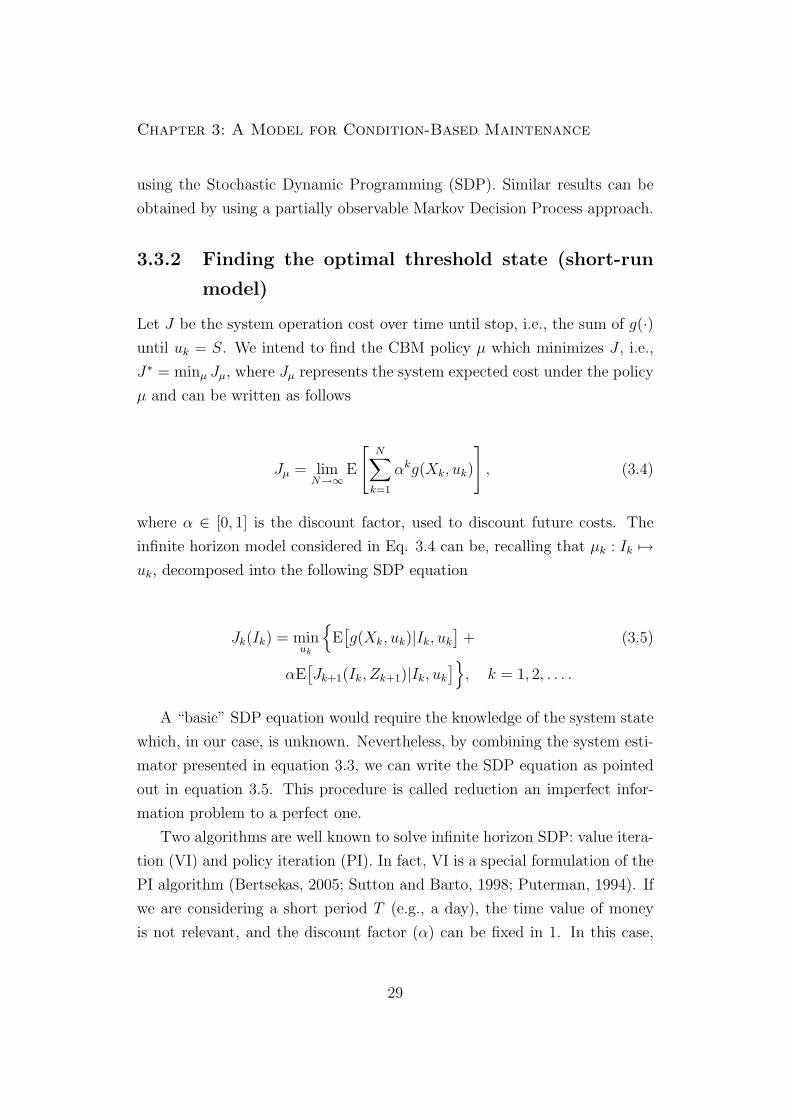
Chapter 3: A Model for Condition-Based Maintenance
using the Stochastic Dynamic Programming (SDP). Similar results can be
obtained by using a partially observable Markov Decision Process approach.
3.3.2 Finding the optimal threshold state (short-run
model)
Let J be the system operation cost over time until stop, i.e., the sum of g(·)until uk = S. We intend to find the CBM policy µ which minimizes J , i.e.,
J∗ = minµ Jµ, where Jµ represents the system expected cost under the policy
µ and can be written as follows
Jµ = limN→∞
E
[N∑k=1
αkg(Xk, uk)
], (3.4)
where α ∈ [0, 1] is the discount factor, used to discount future costs. The
infinite horizon model considered in Eq. 3.4 can be, recalling that µk : Ik 7→uk, decomposed into the following SDP equation
Jk(Ik) = minuk
{E[g(Xk, uk)|Ik, uk
]+ (3.5)
αE[Jk+1(Ik, Zk+1)|Ik, uk
]}, k = 1, 2, . . . .
A “basic” SDP equation would require the knowledge of the system state
which, in our case, is unknown. Nevertheless, by combining the system esti-
mator presented in equation 3.3, we can write the SDP equation as pointed
out in equation 3.5. This procedure is called reduction an imperfect infor-
mation problem to a perfect one.
Two algorithms are well known to solve infinite horizon SDP: value itera-
tion (VI) and policy iteration (PI). In fact, VI is a special formulation of the
PI algorithm (Bertsekas, 2005; Sutton and Barto, 1998; Puterman, 1994). If
we are considering a short period T (e.g., a day), the time value of money
is not relevant, and the discount factor (α) can be fixed in 1. In this case,
29

Chapter 3: A Model for Condition-Based Maintenance
the VI method may require an infinite number of iterations. However, the
method converges finitely under special circumstances. Under definition 1
our problem can be reduced to a Stochastic Shortest-Path (SSP) problem
and, using this fact, we can guarantee the convergence of the VI algorithm,
for α = 1, which will be discussed in the proposition 2. For α < 1, the
convergence is straightforward.
Proposition 2 (Convergence of the value iteration algorithm). Suppose that
the problem is well-defined. Then, the VI algorithm converges with probability
1, since the action uk=S will be taken with finite k.
Proof. Under definition 1, we are able to write the problem as a Stochas-
tic Shortest-Path (SSP) problem (Bertsekas, 2005; Bertsekas and Tsitsiklis,
1991), where the system states are nodes. A SSP problem is a problem in
which the state space {1, 2, . . . , n, t} is such that the node t is a goal (target)
state that is absorbing and cost-free (i.e., Pr[Xk+1 = t|Xk = t] = 1 and
g(t, u) = 0, ∀u), and the discount factor α = 1.
In order to write our problem as a SSP problem, let the states 1, . . . , L be
the nodes 1, . . . , n and create the target node t. This target can be reached
from each state whenever the action u = S is taken (see Fig. 3.6).
Figure 3.6: Stochastic Shortest-Path associated with the problem.
This SSP problem has all cost positives (i) and, with probability 1, the
node t will be reached (ii). Under these two points, it can be shown that the
VI algorithm converges to an optimal and stationary policy (Bertsekas and
Tsitsiklis, 1991; Sutton and Barto, 1998; Bertsekas, 2005), in terms of a SDP
model.
30

Chapter 3: A Model for Condition-Based Maintenance
This algorithm can be used to calculate the optimal repair rule, i.e., deter-
mine the operation threshold r.
3.3.3 The value iteration algorithm
The VI algorithm consists in calculating successive approximations for J∗
through the recursive equations
Jk+1(i) = minu
E[g(Xk+1, u) + Jk(Xk+1)|Xk = i, uk = u
]= min
u
∑j∈X
aij(u)(g(j, u) + Jk(j)), (3.6)
for all i ∈ X. For an arbitrary value of J0, the sequence {Jk}k≥1 converges
to J∗, i.e., |Jk+1(i) − Jk(i)| → 0, ∀i ∈ X, under the same conditions that
guarantee the existence of J∗ (Sutton and Barto, 1998; Bertsekas, 2005).
Algorithm 1 Value iteration algorithm
1: J(i)← 0, ∀i ∈ X . begin with an arbitrary J2: repeat3: ∆← 04: for all i ∈ X do . for all states5: v ← J(i)
6: J(i)← minuk
∑j∈X
pij(u)(g(j, u) + Jk(j))
7: ∆← max(∆, |v − J(i)|)8: until ∆ < ε . precision shall
9: return µ(i) = arg minu
∑j∈X
pij(u)(g(j, u) + J(j))
In addition to the optimal operation threshold r, VI algorithm outputs
the expected cost to termination (J(i)) which, in a SSP context, means that
the state t was reached. In our CBM problem, this cost indicates the expected
cost until the end of a cycle.
31

Chapter 3: A Model for Condition-Based Maintenance
3.4 Model Analytical Properties
In this section we discuss some analytical properties of our CBM model.
Proposition 3 (Our CBM model contemplates both constant and increasing
failure rate in the short-run horizon). In the short-run horizon, if no control
is applied (uk = C, ∀k), the system failure rate is constant or increases over
time.
Proof. If the probabilities a1x = 0 for 2 ≤ x ≤ L−1 we have a constant prob-
ability to failure (a1L) and then a constant failure rate, which is a particular
case. The general case (increasing failure rate) has been proved in 1965 by
Barlow and Proschan4.
In Chapter 5 we provide an illustration of this proposition (page 46).
Despite the Proposition 3 and considering the long-run horizon, the average
uptime is constant: this is the subject of the following result.
Proposition 4 (In the long-run horizon, the number of failures follows a
Renewal Process). In the long-run horizon, if no control is applied (except
that the perfect repair is performed whenever the system fails), the number
of failures follows a Renewal Process.
Proof. Since we consider that the system is left as it is (no control is applied)
and the perfect repair is performed after each failure, the times between
failures are independent and identically distributed (i.i.d.).
Let τ(i, j) be the first passage time in going from state i to state j in a
Markov chain, i.e., the mean length of time required to go from i to j. {Xk}is not ergodic (because of Definition 1 it is not possible to go from state i+ i
to state i) but we only aim to compute the first passage time from state 1
(which is ergodic) since the system starts at this state. τ(1, L) represents
then the time to failure.
4Barlow, R. and Proschan, F. (1965). Mathematical Theory of Reliability. New York:Wiley.
32

Chapter 3: A Model for Condition-Based Maintenance
Let τm(1, L) be the time to failure in the mth short-run horizon. τm(1, L)
are i.i.d. discrete random variables: since no control is applied, there is no
re-estimation of Ψ after each short-run horizon. τm(1, L) have the following
probability distribution:
n pn = Pr[τm(1, L) = n]1 a1L
2 a11a1L + a12a2L
3 a211a1L + a11a12a2L + a12a22a2L + a12a23a3L
......
pn → 0 as n → ∞ because the state L is an absorbing state. Hence,
E[τm(1, L)] is finite and has the same value for all short-run horizon.
In Chapter 5 we also provide an illustration of this result (page 48)
Proposition 5 (A SM policy is a particular case of our CBM model). For
the same system, a SM (Scheduled Maintenance) policy is a particular case
of our CBM policy. Moreover, the SM policy cost is greater or equals to the
CBM policy cost.
Proof. A SM policy can be written as follows:
uk =
{C, if k < n,
S, if k = n,
where n is the period of the scheduled preventive repair. Let W be the system
cost under the SM policy. Since we can write the SM policy as a particular
CBM policy and the CBM policy’s cost is optimal (see Eq. 3.5) we have
W ≥ J,
which demonstrates this result.
33

Chapter 3: A Model for Condition-Based Maintenance
Notice that the information about the system required to apply any CBM
policy may have a cost. We have not considered this case but in practice one
should take it into account when planning the CBM approach.
Proposition 6 (Our CBM policy improves the system availability). The
system availability under our CBM model is greater than or equal to the
availability under a SM policy.
Proof. Recalling the definition of availability (Section 2.1) and fixing the
MTTR (mean time to repair) since it is not concerned (it is assumed to be
the same in both cases), the availability can be increased as the MTTF (mean
time to failure = E[Uptime]) increases.
In order to demonstrate this result, let us set the cost function g as
follows: g(x < L, u = C) = −1, g(x < L, u = S) = 1, g(L, uk = S) = 1 and
g(L, uk=C) = 2. Note that this satisfies Definition 1.
Our Stochastic-Dynamic Programming equation (Eq. 3.5) is designed to
minimize the cost to go from stage k to stage k+1. With g as defined above,
Eq. 3.5 is now an algorithm to maximize the expected number of transitions
of {Xk}.Let W and J be the expected number of transitions under a SM and a
CBM policy, respectively. From Proposition 5 we have
W ≥ J,
which demonstrates this result since both W and J are expected to be ne-
gative numbers (as consequence of cost function g).
34

Chapter 4
Inference of Model Parameters
4.1 Introduction and Motivation
This chapter addresses to the problem of fitting the CBM model parame-
ters to apply the model to a given system. That means we are looking for
a technique that uses the available data and leads to the best parameters
estimation.
The motivation for using Hidden Markov Models (HMM for short) for pa-
rameters estimation comes from its ability to differentiate between changes
in the system measurement which are due to regular system changes (e.g.,
changes of operating conditions), and condition measurement changes which
are due to changes in the measuring instrument and/or measurement pre-
cisions. Also, there exist computationally efficient methods for computing
likelihoods, in particular in the signal processing literature. Additional in-
formation on this topic can be found in (Rabiner, 1989; Ephraim and Merhav,
2002; Dugad and Desai, 1996).
HMM has already been used to tackle maintenance problems. For in-
stance, Tai et al. (2009) use HMM to deal with machine’s production con-
formity in order to detect machine/equipment failures. In line with that
work, Bunks et al. (2000) consider vibration measures to assess the status
of helicopter gearboxes. However, different from our approach, those papers
do not aim to propose CBM policies. Furthermore, we are also interested
expanding the use of CBM policies through HMM by offering an approach
35

Chapter 4: Inference of Model Parameters
for estimating the input parameters.
4.2 Model Parameters Estimation
We deal with the problem of parameters estimation by modeling the available
data for estimating the parameters of our model (Ψ) in order to construct
the statistical inference for Ψ.
Let O represent the historical information about the system, i.e., the
historical data. O can be viewed as a set of M observation sequences, or
observed cycles (as defined in Fig. 3.1). That is O = {O1, O2, . . . , OM},where Om represents a cycle, and it can be written as Om = {z1, z2, . . . , zN},where N is the cycle’s length and zn is the system condition observed in n.
The estimation of Ψ = (A,B) can be viewed as follows: given the available
historical information O, we want to define Ψ as a function of the data
available. In other words, the problem is to find Ψ that maximizes Pr[O|Ψ]1.
We assume that an initial guess of Ψ is available, which will be denoted by
Ψ0.
Unfortunately, there is no known analytical approach to solve maxΨ Pr[O|Ψ]
(Rabiner, 1989). Nonetheless, this problem can be solved numerically using
an iterative procedure. The most successful method, widely cited in the liter-
ature, is the Baum-Welch re-estimation formulas (Baum et al., 1970), which
will be discussed below.
4.2.1 The Baum-Welch Algorithm
“Baum-Welch algorithm” is an algorithm based on successive applications
of the Baum-Welch re-estimation formulas (Baum et al., 1970). The model
Ψ = (A,B) is adjusted so as to increase Pr[O|Ψ] until a maximum value is
reached. First, we offer an intuitive explanation of the formulas.
Let aij and bx(z) be an estimation of aij and bx(z), respectively. These
estimators are based on the relative frequency principle, as follows:
1This problem is called in HMM literature as “problem 3”.
36

Chapter 4: Inference of Model Parameters
• aij =expected number (e.n.) of transition from state i to j
e.n. of transition leaving i;
• bx(z) = e.n. of times in x where z was observede.n. of times in x
.
In order to describe the procedure for re-estimation for each observation
sequence On we define the following variables:
• forward: αn(x) = Pr[Z1 = z1, Z2 = z2, . . . , Zn = zn, Xn = x|Ψ];
• backward: βn(x) = Pr[Zn+1 = zn+1, Zn+2 = zn+2, . . . , ZN = zN , XN =
x|Ψ].
In the previous Chapter, we considered the question of estimating the
system state (Xk) from the information vector (Ik), as described in equation
3.3. The computation of Pr[Xk = x|Ik] can be efficiently performed using
the forward variable:
Pr[Xk = x|Ik] =Pr[Xk = x, Ik]
Pr[Ik]=
αk(x)∑i∈X
αk(i). (4.1)
Now let γn(x) be the probability of being in state x at time n given On
and Ψ, i.e., γn(x) = Pr[Xn = x|On,Ψ]. The use of Bayes rule yields
γk(x) = Pr[Xk = x|On,Ψ] =Pr[Xk = x,On|Ψ]
Pr[On|Ψ]=αk(x)βk(x)
Pr[On|Ψ].
Finally, let ξk(i, j) be the probability of being in the state i at epoch k and
making a transition to j at k+1, i.e., ξk(i, j) = Pr[Xk = i,Xk+1 = j|On,Ψ].
Using the Bayes rule yields
ξk(i, j) =Pr[Xk = i,Xk+1 = j, On|Ψ]
Pr[On|Ψ]=αk(i)aijbj(Zk+1)βk+1(j)
Pr[On|Ψ].
37

Chapter 4: Inference of Model Parameters
It can be shown that∑K−1
k=1 γk(x) is the expected number of transitions
from state x and∑K−1
k=1 ξk(i, j) is the expected number of transitions from
state i to state j (Rabiner, 1989; Dugad and Desai, 1996).
Now, we present the Baum-Welch re-estimation formulas:
• aij =K−1∑k=1
ξk(i, j)/K−1∑k=1
γk(i)
• bx(z) =K∑
k=1zk=z
γk(x)/K∑k=1
γk(x)
We can use these formulas to enhance the estimation quality using the
historical data. That is to say, we start with an initial estimation of Ψ and
we are able to improve this estimation by using field data, which makes our
approach clearly more applicable to real contexts. The algorithm 2 is pro-
posed based on these formulas. It involves collecting a set of data sequences,
computing the posterior distribution over hidden variables (Xk) at all times
given that sequences, and, finally, updating the parameters according to the
statistics of the posterior distribution.
Algorithm 2 Baum-Welch algorithm
1: Ψ0 ← (A,B) . a priori estimate for Ψ2: for all n ∈ 1..N do . for each observation sequence
3: aij ←K−1∑k=1
ξk(i, j)/K−1∑k=1
γk(i), ∀i, j ∈ X
4: bx(z)←K∑
k=1zk=z
γk(x)/K∑k=1
γk(x), ∀x ∈ X, ∀z ∈ Z
5: Ψn ← (aij, bx(z))
6: return ΨN
Applying this algorithm at the end of each cycle (as described in Fig.
3.2) yields a systematic updating of Ψ, which is suitable for computer im-
plementation as part of a maintenance software, for example. Consequently,
we are able to get a more accurate estimation of Ψ as soon as more data are
available.
38

Chapter 4: Inference of Model Parameters
4.3 Estimation Properties
The Baum-Welch algorithm is a computationally efficient iterative algorithm
for local maximization of the log-likelihood function. For more details, please
check (Ephraim and Merhav, 2002). It is an expectation-maximization al-
gorithm and it was developed and proved to local converge by Baum et al.
(1970).
In this section, we present some characteristics of our inference model
based on the Baum-Welch algorithm. To this end, let us define the following
terms for a given system2:
• Ψ: the system’s real parameters;
• Ψ0: initial guess of the system’s parameters;
• ΨN : the estimation of the system’s parameters yielded by the Baum-
Welch algorithm after running N observation sequences.
We can use Ψ to generate N random samples in order to simulate Baum-
Welch algorithm and evaluate its fitting quality. Formally, this is called sta-
tistical simulation and it means an artificial data generation process, driven
by model design and parameter settings. The output, a synthetic sample,
can be used to validate the inference process.
For the purpose of evaluate the bias between Ψ and ΨN , let us create the
following fitness measure
ρ =∑i,j∈X
(aij − aij)2 +∑
x∈X,z∈Z
(bx(z)− bx(z))2. (4.2)
Hence, ρ is the sum of the squared residual deviations between Ψ and ΨN
for both transition (A) and observation (B) probability matrices.
Proposition 7 (Baum-Welch algorithm convergence depends on the initial
parameters guess). The Baum-Welch algorithm gives an estimation that cor-
responds to the local maximum of the likelihood function. However, there
2Please recall that the system is assumed to be well-defined (Definition 1).
39

Chapter 4: Inference of Model Parameters
exists at least one Ψ0 which garantees the convergence (global maximum of
the likelihood function) to the real system’s parameters as the number of em-
pirical data increases. That is
∃Ψ0 : ρN→∞−→ 0. (4.3)
Proof. Finding a Ψ0 that results in the algorithm convergence is straightfor-
ward: Baum-Welch will always converge if we make Ψ0 = Ψ for a sufficiently
larger N .
Indeed, the key question is how to choose the initial guess Ψ0 so that the
local maximum is the global maximum of the likelihood function. If it does
not happen, the algorithm yields a suboptimal solution. This fact is due to
the Baum-Welch formulas structure (Ephraim and Merhav, 2002; Rabiner,
1989; Baum et al., 1970) and basically there is no simple answer. We provide
below examples showing optimal and suboptimal convergences.
Let us illustrate the Proposition 7. For this purpose, we performed the
following experiment:
Algorithm 3 Baum-Welch convergence test: unbiased Ψ0 case
1: generate L as a discrete uniform distribution in [2, 10]2: create Ψ as follows: (it assures that all probabilities add to 1 when needed
and Ψ will be well-defined)
• aii = 0.94 for 1 ≤ i < L−1, aL−1L−1 = 0.95 and aLL = 1
• aii+1 = 0.05 for 1 ≤ i < L
• b1(1) = 0.9, bx(z) = 0.8 for 1 < x < L, 1 < z < L and bL(L) = 0.9
• bii+1 = 0.1 for 1 ≤ i < L and bii−1 = 0.1 for 1 < i ≤ L
3: let Ψ0 = Ψ, i.e., a completely unbiased prior estimation4: generate N random data series from Ψ. Each series corresponds to a
complete simulation of the system running to failure, i.e., the series endswhenever L is reached
5: for each series n ∈ N , we use Baum-Welch to get Ψn and then we evaluateρ according to Eq. 4.2.
The Fig. 4.1 presents the results: it shows ρ→ 0 when N grows.
40

Chapter 4: Inference of Model Parameters
Figure 4.1: Baum-Welch optimal convergence for some random data (10runs).
This result shows a cleary convergence of the method. Let us now run
our experiment considering a “uniform” prior system parameters estimation
(Ψ0). We replace then line 3 in Alg. 3 by:
Algorithm 4 Baum-Welch convergence test: uniform Ψ0 case
create Ψ0 as follows:for i = 1 to L do
for j = i to L do . starts from i to ensure “well-definedness”
aij =1
L− i+ 1. uniform distribution
for x = 1 to L dofor z = 1 to L do
bx(z) =1
L. uniform distribution
This piece of pseudo-code produces an “uniform” Ψ0. Running again our
experiment produces the Fig. 4.2. We have limited the number of generated
data series (N) to 50 due the computational effort required to run the Baum-
Welch algorithm. In one case we have an optimal estimation (L = 3).
The Fig. 4.3 shows a long-run using an “uniform” Ψ0 converging to a non-
41

Chapter 4: Inference of Model Parameters
Figure 4.2: Baum-Welch suboptimal convergence for some random data (10runs).
optimal estimation since ρ 9 0. This test required about 3hs of machine3.
Figure 4.3: Baum-Welch suboptimal convergence for some random data (1run).
Rabiner (1989) points out that the initial guess of the matrixB is specially
3The computational environment is described in the beginning of the Chapter 5.
42

Chapter 4: Inference of Model Parameters
critical. To illustrate this fact, let us replace the part of Alg. 4 that generates
B by the following:
Algorithm 5 Baum-Welch convergence test: “semi-unbiased” B-matrix case
for x = 1 to L dofor z = 1 to L do
if observation z corresponds to x (as in 1 = 1) thenbx(z) = 0.5
else
bx(z) =0.5
L− 1. “uniform” distribution
Hence, we give a half of the probability mass to the correct guess. The
rest of B is left uniformly random. The results are sensibily differents: all
estimations have optimally converged (see Fig. 4.4).
Figure 4.4: Baum-Welch optimal convergence for some random data (10runs).
This section highlights the role of the initial parameters guess in the
parameters estimation as a whole. Rabiner (1989) says that there is no
general answer but there exist some techniques useful, though, helping to
avoid suboptimals estimation regardless the initial guess. For the purposes
of this dissertation, this topic will not be covered.
43

Chapter 5
An Application Example
This chapter discusses the application of our methodology using empiric data.
The algorithms were coded using Matlab v6.5 and the tests were performed
on a 2.0 GHz dual core machine with 3Gb RAM running Microsoft Windows
XP. All computation times took no more than 10 seconds.
5.1 Preliminaries
Our application example uses data from a piece of equipment, provided by
a zinc mining company. For confidentiality reasons, we have had to disguise
the input data1. This system is electric-powered, it runs continuously, and
its main failure mode is a serious internal degradation, affecting the product
quality and the process productivity. This failure can happen whenever the
electric current is higher than a given design-fixed value, which is supposed
to be the maximum value for a correct operation. The perfect repair is per-
formed by replacing some internal components. Upon failure, even while the
piece of equipment is still running, the degradation is generalized, requiring
a more complex repair.
We wish to define the state failed (L) as the state where we have to carry
out the complex repair in order to bring back the system to state 1. Therefore,
in some sense, the event failure is hidden since it does not necessarily imply
1It has been performed by multiplying all values by some constant in such a way that,despite the changes, the data remain coherent.
44

Chapter 5: An Application Example
that the piece of equipment is broken or not operating. Because of equipment
design and structure, as well as operational limitations, the electric current
is the monitored parameter. It is assumed that other failure modes are not
relevant and that they have no correlation with the mode being analyzed.
Hence, let θk denote the current measured (in Ampere) at epoch k, sampled
every day (the period T ). We set L = 5 and Table 5.1 shows the classification
adopted in our study, translating the parameter measurement into condition
measurement.
Parameter value zkθk < 27.5 1
27.5 ≤ θk < 29.0 229.0 ≤ θk < 30.5 330.5 ≤ θk < 32.0 4
θk ≥ 32.0 5 (system seems failed)
Table 5.1: Classification of the parameter measurement.
The cost function g(xk, uk) considered is showed in Table 5.2. Notice
that “stop and perform the preventive maintenance” (g(xk, uk) with xk =
{1, 2, 3, 4}, uk = S) is 50 times more expensive than operate the system in
the condition “as good as new” (g(xk, uk) with xk=1, uk=C). For reference
purposes, let us call this function as gA.
Action taken (uk)System real condition (xk) Continue Stop
1 1 502 1.1 503 1.2 504 1.3 50
5 (failed) 1000 200
Table 5.2: The cost function gA.
45

Chapter 5: An Application Example
5.2 Initial Parameters Estimation
We discuss now the model parameters (Ψ) estimation. As discussed, we
need an initial guess of Ψ, showed in Fig. 5.1. This estimation considers the
wear-out process and the possibility of failures due to shocks as well.
Figure 5.1: The initial guess (Ψ0) of the transition and observation matrices.
Let us illustrate some properties of our model. If the system is left “as
it is” (no control is applied), we expect that the system will fail in a finite
time interval due to wear-out and shock failures. We can check this fact by
computing the reliability and failure rate functions using Ψ0, as in Figs. 5.2
and 5.3.
Figure 5.2: The reliability function for the system (Ψ0) if no control is ap-plied.
46

Chapter 5: An Application Example
Figure 5.3: The failure rate function for the system (Ψ0) if no control isapplied.
We have an increasing failure rate, which is the general case by systems
modeled using Markov chains, as discussed in Proposition 3. Since we con-
sider discrete-time Markov chain, we have computed the failure rate λ(k)
with respect to a fixed interval equal to 1 (a day, the period T ). This system
deterioration can be verified by computing the n-step transition probability
matrices, as shown in Table 5.3.
A10:
0.5386 0.2865 0.0686 0.0099 0.09640 0.5386 0.2865 0.0706 0.10430 0 0.5386 0.3006 0.16080 0 0 0.5987 0.40130 0 0 0 1.0000
A100:
0.0021 0.0109 0.0288 0.0661 0.89220 0.0021 0.0109 0.0420 0.94500 0 0.0021 0.0193 0.97860 0 0 0.0059 0.99410 0 0 0 1.0000
A500:
0.0000 0.0000 0.0000 0.0000 1.00000 0.0000 0.0000 0.0000 1.00000 0 0.0000 0.0000 1.00000 0 0 0.0000 1.00000 0 0 0 1.0000
Table 5.3: Some n-step transition probability matrices if no control is applied.
Still considering that no control is applied, we can compute the distribu-
tion of the time to failure (τ(1, L), Proposition 4). For this purpose, we use
47

Chapter 5: An Application Example
Ψ0 to calculate τ(1, L), as in Fig 5.4.
Figure 5.4: The distribution of the time to failure (τ(1, L)) for the system(Ψ0) if no control is applied.
The data set used for initial parameters estimation consists of 3 distinct
systems that are in the same operating condition, in a total of 11 series. Ac-
cording to our definition of failure, two of these series are of the “up to pre-
ventive maintenance” type (Fig. 3.1a), while the others are of the “through
failure” type. The Fig. 5.5 illustrates, for each series, the behavior of the
electric current over time and Fig. 5.6 shows the data after classification,
performed according to Table 5.1.
Figure 5.5: The data series (total: 11) used in our application example.
We use these data series in our Hidden Markov Model approach to construct
the statistical inference for Ψ, providing a better estimation given the his-
torical data available.
48
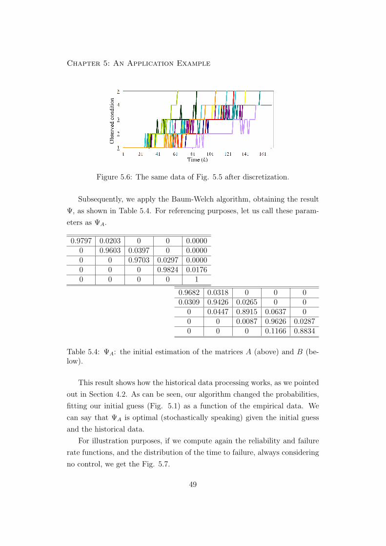
Chapter 5: An Application Example
Figure 5.6: The same data of Fig. 5.5 after discretization.
Subsequently, we apply the Baum-Welch algorithm, obtaining the result
Ψ, as shown in Table 5.4. For referencing purposes, let us call these param-
eters as ΨA.
0.9797 0.0203 0 0 0.00000 0.9603 0.0397 0 0.00000 0 0.9703 0.0297 0.00000 0 0 0.9824 0.01760 0 0 0 1
0.9682 0.0318 0 0 00.0309 0.9426 0.0265 0 0
0 0.0447 0.8915 0.0637 00 0 0.0087 0.9626 0.02870 0 0 0.1166 0.8834
Table 5.4: ΨA: the initial estimation of the matrices A (above) and B (be-low).
This result shows how the historical data processing works, as we pointed
out in Section 4.2. As can be seen, our algorithm changed the probabilities,
fitting our initial guess (Fig. 5.1) as a function of the empirical data. We
can say that ΨA is optimal (stochastically speaking) given the initial guess
and the historical data.
For illustration purposes, if we compute again the reliability and failure
rate functions, and the distribution of the time to failure, always considering
no control, we get the Fig. 5.7.
49

Chapter 5: An Application Example
Figure 5.7: The reliability (top) and failure rate (middle) functions, and thedistribution of time to failure (bottom) for ΨA if no control is applied.
Now that we have ΨA, we are able to calculate the CBM policy µ, we
are interested in computing the threshold state (r) by solving the Eq. 3.5
as discussed in Section 3.3. The algorithm result, depicted in Table 5.5,
indicates the state 4 as the threshold state. The expected cost until stop
(preventive or corrective) is 168.8720.
State (Xk) 1 2 3 4(=r) 5Action (uk) C C C S S
Table 5.5: Threshold state (r) computation and optimal action.
We are now prepared to apply our CBM policy µ. We illustrate its application
50

Chapter 5: An Application Example
via the following scenarios that illustrate how our proposed approach works.
5.3 Testing-Scenarios
5.3.1 Scenario 1: A Typical Scenario
We begin by analyzing the scenario illustrated in Fig. 5.8. This figure shows
the behavior of µ: while k < 85, Xk < r= 4 hence uk = C. At k = 85 we
have Xk = 4 and hence u85 = S.
Figure 5.8: Scenario 1: condition observed (top) and state estimation (bot-tom).
Let us illustrate how Eq. 3.3 works: until k = 19 we have Zk = 1 and
(x, Pr[Xk = x|Ik]) as follows: (1, 0.9993), (2, 0.0007); At k = 20, Zk = 2
and (1, 0.6116), (2, 0.3883), (3, 0.0001); At k = 21, Zk = 2 and (1, 0.0497),
(2, 0.9485), (3, 0.0018); ...; At k = 25, Zk = 2 and (2, 0.9979), (3, 0.0021);
At k = 26, Zk = 1 and (1, 0.0001), (2, 0.9999); At k = 25, Zk = 2 and (2,
0.9980), (3, 0.0020).
Since we stopped the system at k = 85, the actual measurement cycle
has just been closed. We wish to update ΨA using the newest condition
measurement series, as described in Fig. 3.2. To this end, we apply Baum-
Welch with the recently updated historical data (Fig. 5.6 plus Fig. 5.8)
giving a new up to now parameters estimation ΨB shown in Table 5.6.
51

Chapter 5: An Application Example
0.9786 0.0214 0 0 00 0.9625 0.0375 0 0.00000 0 0.9696 0.0304 0.00000 0 0 0.9824 0.01760 0 0 0 1
0.9693 0.0307 0 0 00.0299 0.9308 0.0393 0 0
0 0.0445 0.8945 0.0605 00 0 0.0092 0.9625 0.02830 0 0 0.1216 0.8784
Table 5.6: ΨB: the matrices A (above) and B (below) updated (ΨA + Fig.5.8).
5.3.2 Scenario 2: Changes in the Cost g(·)
In this scenario we assume operational costs that are higher than those con-
sidered in gA, as follows: g(1, uk=C) = 1, g(2, uk=C) = 1.5, g(3, uk=C) =
2, g(4, uk =C) = 3 and g(5, uk =C) = 1000; and g(i, uk =S) = 50 (for i≤4)
and g(5, uk=S) = 200. Let us call it as gB(.).
Re-computing the CBM policy µ (using the ΨA, i.e., Table 5.4) yields,
with this new cost function (gB(.)), the state 3 as the threshold state. The
expected cost until stop is 172.7884. As we had expected, this cost is higher
than the cost of the previous scenario.
Hence, it is expected that uk = S will be carried out earlier, as far
as system degradation is concerned, than the state defined in the previous
scenario, reflecting the fact that operating in one of degraded states is more
expensive than before.
5.3.3 Scenario 3: Incidence of Shocks
Let us consider gA and ΨA. Hence, we have µ as in Table 5.5. So far, in the
scenarios we have considered, we did not note the occurrence of shocks. Let
us now analyze the scenario illustrated in Fig. 5.9. As can be seen, there has
been a shock at k = 14 forcing a corrective repair. Therefore, we conducted
52
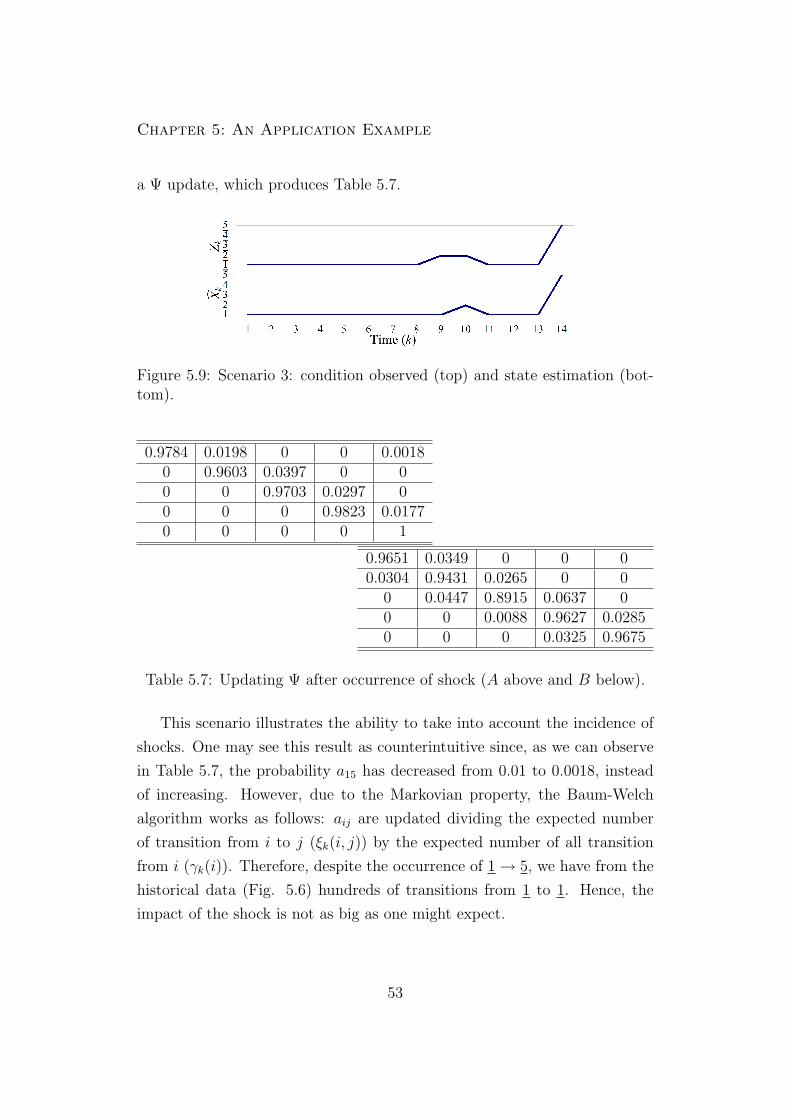
Chapter 5: An Application Example
a Ψ update, which produces Table 5.7.
Figure 5.9: Scenario 3: condition observed (top) and state estimation (bot-tom).
0.9784 0.0198 0 0 0.00180 0.9603 0.0397 0 00 0 0.9703 0.0297 00 0 0 0.9823 0.01770 0 0 0 1
0.9651 0.0349 0 0 00.0304 0.9431 0.0265 0 0
0 0.0447 0.8915 0.0637 00 0 0.0088 0.9627 0.02850 0 0 0.0325 0.9675
Table 5.7: Updating Ψ after occurrence of shock (A above and B below).
This scenario illustrates the ability to take into account the incidence of
shocks. One may see this result as counterintuitive since, as we can observe
in Table 5.7, the probability a15 has decreased from 0.01 to 0.0018, instead
of increasing. However, due to the Markovian property, the Baum-Welch
algorithm works as follows: aij are updated dividing the expected number
of transition from i to j (ξk(i, j)) by the expected number of all transition
from i (γk(i)). Therefore, despite the occurrence of 1→ 5, we have from the
historical data (Fig. 5.6) hundreds of transitions from 1 to 1. Hence, the
impact of the shock is not as big as one might expect.
53

Chapter 5: An Application Example
5.3.4 Scenario 4: Changing L and Classification Step
Let us now illustrate a scenario in which the discretization of the system
condition is refined - that is, a scenario where we take into account higher
values for L. Recall that L is the number of system states between “as good
as new” and “completely failed”. Let’s set L = 10. Fig. 5.10 shows the same
data presented in Fig. 5.5 after new classification, performed according to
Table 5.8.
Parameter value zkθk < 25.25 1
25.25 ≤ θk < 26.00 2(...)
31.25 ≤ θk < 32.0 9θk ≥ 32.0 10 (system seems failed)
Table 5.8: Classification of the parameter measurement.
Figure 5.10: The same data of Figure 5.5 after new discretization (Table 5.8).
We consider an initial guess Ψ and a cost function g similar to the ones
used in scenario 1, just adapted to this scenario where L = 10. Hence,
for A we have aii:i≤8 = 0.94, a99 = 0.95, a1010 = 1, aij:j=i+1,i≤9 = 0.05
and ai10:i≤8 = 0.01. For B we have b1(1) = 0.9, bi(i) = 0.8 (for i ≤ 9)
and b10(10) = 0.9; bi(i+1) = 0.1 (for i ≤ 9) and bi+1(i) = 0.1 (for i ≤ 9).
The cost function is the following: g(1, uk = C) = 1, g(2, uk = C) = 1.1,
g(3, uk = C) = 1.2, ..., g(9, uk = C) = 1.8 and g(10, uk = C) = 1000; and
g(i, uk=S) = 50 (for i≤9) and g(10, uk=S) = 200.
54

Chapter 5: An Application Example
Applying Baum-Welch for parameters estimation yields the state 7 as
threshold state. The expected cost until stop is 272.6329. In Fig. 5.11 we
present the same data used in scenario 1 using the new classification. In this
case, we stop the system at k = 71 since Xk = 7. As should be expected,
setting L = 10 implies different results from the model using L = 5.
Figure 5.11: Scenario 4: condition observed and state estimation.
55

Chapter 6
Conclusion, Suggestions for
Future Research
In this dissertation, we have studied the problem of constructing Condition-
Based Maintenance policy for systems under periodic inspection. The system
state is represented by a discrete-state Markov process and we take into ac-
count that the condition measurement may be not perfect. Also, we have
discussed the model parameters inference from a both theoretical and prac-
tical point of view.
The main result of this dissertation is a framework that combines opti-
mization and model parameter computation from historical data. We illus-
trated the application of our methodology in a industrial case and provided
a step by step discussion of our approach, using four different scenarios, illus-
trating its key points. The result suggests an approach suitable for industrial
applications, which can help managers to improve their decisions for cases
similar to the one that we tackled.
Few papers in the literature have pointed out that the Hidden Markov
Model theory is efficient to model historical data concerning condition mea-
surement. This dissertation expands the use of HMMs in reliability and
maintenance field by combining an optimization model with input parame-
ters estimation from empirical data. We believe our work can increase the
use of such models as well as motivate more research in this area.
An important issue of our approach concerns the parameters’ estimation
56

Chapter 6: Conclusion, Suggestions for Future Research
robustness, since this step critically determines the CBM model outputs as
well as the performance and effectiveness of the model outcome. We have
chosen HMM because of its solid mathematical structure and theoretical
basis, as well as the computational efficiency to compute the estimations.
However, some aspects of HMM were not explored – for instance, a formal
discussion concerning the quality of the parameter estimates provided by the
Baum-Welch algorithm.
There are a couple of extensions, refinements, and alternative formula-
tions that might be worth exploring. As a future work, one can plan to im-
prove on our approach by considering some sophistication, we suggest some
possible directions:
1. Use of intermediate repairs, such as the minimal one. For instance, a
minimal repair will bring the system back to the state it was just after
failure.
2. Consider the stochastic rejuvenation. In this case, the repair action
outcome is stochastic, i.e., the state that the system will be brought is
a probability distribution.
3. Use random or sequential inspection (periodic inspection is a particular
case). One should also consider the cost do obtain information about
the system condition through inspection or any other mean (such as
on-line monitoring using sensors).
Naturally, these refinements would increase the complexity and thus would
require a different approach to process historical data for estimation of model
parameters.
57

Bibliography
Barlow, R. and Hunter, L. (1960). Optimum preventive maintenance policies.
Operations Research, 8:90–100.
Baum, L. E., Petrie, T., Soules, G., and Weiss, N. (1970). A maximization
technique occurring in the statistical analysis of probabilistic functions of
markov chains. The Annals of Mathematical Statistics, 41(1):164–171.
Bellman, R. E. (1957). Dynamic Programming. Princeton: Princeton Uni-
versity Press.
Bertsekas, D. P. (2005). Dynamic Programming and Optimal Control, 3rd
edition. Belmont: Athena Scientific.
Bertsekas, D. P. and Tsitsiklis, J. N. (1991). An analysis of stochastic shortest
path problems. Mathematics of Operations Research, 16:580–595.
Bloch-Mercier, S. (2002). A preventive maintenance policy with sequential
checking procedure for a markov deteriorating system. European Journal
of Operational Research, 147:548–576.
Bloom, N. B. (2006). Reliability-Centered Maintenance. New York: Mac
Graw-Hill).
Bunks, C., McCarthy, D., and Al-Ani, T. (2000). Condition-based mainte-
nance of machines using hidden markov models. Mechanical Systems and
Signal Processing, 14:597–612.
58

Bibliography
Cassandras, C. G. and Lafortune, S. (2009). Introduction To Discrete Event
Systems, 2nd edition. New York: Springer.
Charng, T. (1981). Optimum equipment maintenance/replacement policy
periodic inspection of a stochastically degrading system. Technical Report
42-66, TDA Progress Report, NASA, USA.
Chen, C. T., Chen, Y. W., and Yuan, J. (2003). On a dynamic preventive
maintenance policy for a system under inspection. Reliability Engineering
and System Safety, 80:41–47.
Chen, D. and Trivedi, K. S. (2005). Optimization for condition-based main-
tenance with semi-markov decision process. Reliability Engineering and
System Safety, 90:25–29.
Chiang, J. H. and Yuan, J. (2001). Optimal maintenance policy for a marko-
vian system under periodic inspection. Reliability Engineering and System
Safety, 71:165–172.
Dugad, R. and Desai, U. B. (1996). A tutorial on Hidden Markov Mod-
els. Technical Report n◦. SPANN-96.1, Indian Institute of Technology -
Bombay.
Ephraim, Y. and Merhav, N. (2002). Hidden markov processes. IEEE Trans-
actions on Information Theory, 48(6):1518–1569.
Gong, L. and Tang, K. (1997). Monitoring machine operations using on-line
sensors. European Journal of Operational Research, 96:479–492.
Grate, L. et al. (2006). Stochastic modeling techniques: under-
standing and using Hidden Markov Models. Tutorial available in
http://compbio.soe.ucsc.edu/papers/ismb96 tutorial.ps.
Grimmett, G. and Stirzaker, D. (2001). Probability and Random Processes,
3rd edition. New York: Oxford University Press.
59

Bibliography
Gurler, U. and Kaya, A. (2002). A maintenance policy for a system with
multi-state components: an approximate solution. Reliability Engineering
and System Safety, 76:117–127.
Hoel, P. G., Port, S. C., and Stone, C. J. (1972). Introduction to Stochastic
Processes. Prospect Heights: Waveland Press.
Kawai, H., Koyanagi, J., and Ohnishi, M. (2002). Stochastic Models in
Reliability and Maintenance, chapter Optimal Maintenance Problems for
Markovian Deteriorating Systems, pages 193–218. Berlin: Springer.
Lam, C. T. and Yeh, R. H. (1994). Optimal maintenance-policies for deteri-
orating system under various maintenance strategies. IEEE Transactions
on Reliability, 43:423–430.
Moubray, J. (1993). Reliability-Centered Maintenance. New York: Industrial
Press).
Nakagawa, T. (2005). Maintenance Theory Of Reliability. Springer Series in
Reliability Engineering. London: Springer.
Ohnishi, M., Moriokab, T., and Ibaraki, T. (1994). Optimal minimal-repair
and replacement problem of discrete-time markovian deterioration system
under incomplete state information. Computers & Industrial Engineering,
27:409–412.
Pham, H. (2003). Handbook of Reliability Engineering. London: Springer.
Pierskalla, W. P. and Voelker, J. A. (1976). A survey of maintenance mod-
els: the control and surveillance of deteriorating systems. Naval Research
Logistics Quartely, 23:353–388.
Puterman, M. L. (1994). Markov Decision Processes. New York: John Wiley
& Sons.
Rabiner, L. R. (1989). A tutorial on hidden markov models and selected
applications in speech recognition. In Proceedings of the IEEE, volume 77,
pages 257–286.
60

Bibliography
Rigdon, S. E. and Basu, A. P. (2000). Statistical Methods for the Reliability
of Repairable Systems. New York: John Wiley & Sons.
Sherif, Y. S. and Smith, M. L. (1981). Optimal maintenance models for
systems subject to failure - a review. Naval Research Logistics, 28:47–74.
Smith, A. M. (1993). Reliability-Centered Maintenance. New York: Mac
Graw-Hill.
Sutton, R. S. and Barto, A. G. (1998). Reinforcement Learning: An Intro-
duction. Cambridge: The MIT Press.
Tai, A. H., Ching, W.-K., and Chan, L. (2009). Detection of machine failure:
Hidden markov model approach. Computers & Industrial Engineering,
57:608–619.
Valdez-Flores, C. and Feldman, R. M. (1989). A survey of preventive main-
tenance models for stochastically deteriorating single-unit system. Naval
Research Logistics, 36:419–446.
Wang, H. and Pham, H. (2006). Reliability and Optimal Maintenance.
Springer Series in Reliability Engineering. London: Springer.
Wang, L., Chu, J., and Mao, W. (2008). A condition-based order-replacement
policy for a single-unit system. Applied Mathematical Modelling, 32:2274–
2289.
61