Relief Texture Mapping

TR00-009

March 3, 2000�Manuel Menezes de Oliveira Neto

Department of Computer Science

University of North Carolina at Chapel Hill

Chapel Hill, NC 27599-3175 �UNC is an Equal Opportunity/A�rmative Action Institution.

RELIEF TEXTURE MAPPING

by

Manuel Menezes de Oliveira Neto

A dissertation submitted to the faculty of the University of North Carolina at Chapel Hill

in partial fulfillment of the requirements of the degree of Doctor of Philosophy in the

Department of Computer Science.

Chapel Hill

March 2000

Approved by:

ii

This page left blank intentionally.

iii

© 2000Manuel Menezes de Oliveira Neto

ALL RIGHTS RESERVED

iv

This page left blank intentionally.

v

ABSTRACTManuel Menezes de Oliveira Neto

Relief Texture Mapping(Under the supervision of Professor Gary Bishop)

This dissertation presents an extension to texture mapping that supports the

representation of 3-D surface details and view motion parallax. The results are correct for

viewpoints that are static or moving, far away or nearby. In this approach, a relief texture

(texture extended with an orthogonal displacement per texel) is mapped onto a polygon

using a two-step process. First, it is converted into an ordinary texture using a

surprisingly simple 1-D forward transform. The resulting texture is then mapped onto the

polygon using standard texture mapping. The 1-D warping functions work in texture

coordinates to handle the parallax and visibility changes that result from the 3-D shape of

the displacement surface. The subsequent texture-mapping operation handles the

transformation from texture to screen coordinates.

The pre-warping equations have a very simple 1-D structure that enables the pre-

warp to be implemented using only 1-D image operations along rows and columns and

requires interpolation between only two adjacent texels at a time. This allows efficient

implementation in software and should allow a simple and efficient hardware

implementation. The texture-mapping hardware already very common in graphics

systems efficiently implements the final texture mapping stage of the warp.

I demonstrate a software implementation of the method and show that it

significantly increases the expressive power of conventional texture mapping. It also

dramatically reduces the polygon count required to model a scene, while preserving its

realistic look. This new approach supports the representation and rendering of three-

dimensional objects and immersive environments, and naturally integrates itself with

popular graphics APIs. An important aspect of this research is to provide a framework for

combining the photo-realistic promise of image-based modeling and rendering techniques

with the advantages of polygonal rendering.

vi

This page left blank intentionally.

vii

ACKNOWLEDGEMENTS

Very special thanks go to my advisor, Gary Bishop, for his enthusiasm, friendship and for

the many delightful discussions we’ve had. His insightful remarks and suggestions were

invaluable for me during this project and are a source of inspiration that will last much

longer than this dissertation.

I would also like to warmly acknowledge the other members of my dissertation

committee: Professors Frederick Brooks, Nick England, Anselmo Lastra, Steve Molnar

and Lars Nyland. All these gentlemen have contributed valuable suggestions to this work.

Lars was especially encouraging to me during the planning stages of this thesis.

Professors Anatólio Laschuk and Elian Machado deserve warm recognition for their

earlier support and inspiration.

The following people have provided me with various kinds of assistance as I worked in

this project. David McAllister assisted with the production of some animations. Voicu

Popescu lent me a 3-D Studio MAX® plug-in. Paul Rademacher provided GLUI. Cassio

Ribeiro designed Relief Town. David, Lars, Voicu, Anselmo and Chris McCue provided

the reading room data set. Jason Smith let me borrow his voice and accent for video

submissions, and George Stackpole proofread this dissertation. de Espona Infografica

created most of the 3-D models I used.

During the undertaking of this project, the Computer Science Department faculty and

staff provided a wonderful working environment. Janet Jones and Mary Whitton deserve

special recognition for their assistance.

Additionally, I would like to acknowledge the Brazilian Research Council (CNPq –

process # 200054/95) for supporting me during my graduate studies. DARPA and NSF

have also provided some funding.

Finally, I want to extend my heartfelt gratitude to my mother and to Ninha, for showing

me so much love, and to my wife, Ana, for all her love, patience and support.

viii

This page left blank intentionally.

ix

To my lovely wife,

To all our children,

And to their children, too.

x

This page left blank intentionally.

xi

TABLE OF CONTENTS

LIST OF TABLES ........................................................................................................ xv

LIST OF FIGURES ...................................................................................................xvii

LIST OF EQUATIONS .............................................................................................xxiii

CHAPTER 1 – INTRODUCTION ....................................................................... 1

1.1 Hybrid Systems............................................................................................................. 4

1.2 Thesis Statement……………………………………………………….……..………4

1.3 Results………………………………………………………………………….……..6

1.4 Overview of the Relief Texture Mapping Algorithm................................................... 7

1.5 Related Work............................................................................................................. 8

1.5.1 Image warping methods ................................................................................... 9

1.5.2 View-dependent texture mapping .................................................................. 10

1.5.3 One-dimensional Perspective Projection ....................................................... 10

1.5.4 Extension for handling visibility.................................................................... 10

1.6 Discussion................................................................................................................... 11

CHAPTER 2 – SEPARABLE TRANSFORMATIONS................................... 13

2.1 Images and Warp Maps .............................................................................................. 13

2.2 Parallel and Serial Warps ........................................................................................... 15

2.3 Difficulties Associated with Serial Warps.................................................................. 17

2.3.1 Bottlenecks ..................................................................................................... 17

2.3.2 Foldovers........................................................................................................ 23

2.4 The Ideal Separable Transform .................................................................................. 25

2.5 Intensity Resampling .................................................................................................. 26

2.5.1 One-dimensional intensity resampling........................................................... 26

2.5.2 Limitations of one-dimensional serial resampling ......................................... 27

2.6 Discussion................................................................................................................... 28

xii

CHAPTER 3 – RELIEF TEXTURE MAPPING AND THE PRE- WARPINGEQUATIONS ............................................................................. 31

3.1 Images with Depth and Relief Textures ..................................................................... 32

3.2 3-D image Warping .................................................................................................... 34

3.3 Factoring the 3-D Image-Warping Equation.............................................................. 59

3.4 The Ideal Factorization............................................................................................... 39

3.5 Simpler Coefficients ................................................................................................... 42

3.6 Pre-warping Equations for Relief Textures ................................................................ 43

3.6.1 The one-dimensional nature of the pre-warping equations............................ 46

3.6.2 Geometric interpretation of the coefficients of the pre-warping equations forrelief textures ................................................................................................. 51

3.6.3 A Useful identity............................................................................................ 51

3.6.4 Pre-warping equations for perspective projection source images: a geometricderivation ....................................................................................................... 52

3.7 Occlusion-Compatible Order for Parallel Projection Images with Depth.................. 54

3.8 Pre-Warping Equations for Inside-Looking-Out Cells ........................................... 79

3.9 Discussion ............................................................................................................... 59

CHAPTER 4 – IMAGE RESAMPLING FROM RELIEF TEXTURES ....... 63

4.1 Two-Pass 1-D Resampling ......................................................................................... 64

4.1.1. Limitations of the straightforward two-pass 1-D warp .................................. 664.1.1.1 Self-occlusion errors .................................................................................. 66

4.1.1.2 Color interpolation errors ........................................................................... 67

4.1.1.3 Non-linear distortion.................................................................................. 69

4.1.2 Correcting the non-linear effects of the interpolation.................................... 71

4.1.2.1 Asymmetric two-pass algorithm................................................................ 72

4.1.2.2 Two-pass algorithm with displacement compensation .............................. 74

4.2 Pipelined Resampling.............................................................................................. 75

4.3 Mesh-Based Resampling......................................................................................... 77

4.4 Reconstruction Using Quantized Displacement Values.......................................... 79

4.5 Rendering Statistics................................................................................................. 81

4.6 Filtering Composition ............................................................................................. 82

4.7 The Changing Field of View Effect ........................................................................... 83

4.8 Discussion................................................................................................................... 87

xiii

CHAPTER 5 – OBJECT AND SCENE MODELING AND RENDERING .. 89

5.1 Multiple Instantiations of Relief Textures.................................................................. 89

5.2 Capturing Samples Beyond the Limits of the Source Image Plane............................ 91

5.3 Object Representation ............................................................................................. 93

5.4 Handling Surface Discontinuities............................................................................ 97

5.5 Correct Occlusions .................................................................................................. 98

5.6 Scene Modeling..................................................................................................... 103

5.7 Discussion................................................................................................................. 106

CHAPTER 6 – MULTIRESOLUTION, INVERSE PRE-WARPING,CLIPPING AND SHADING .................................................. 111

6.1 Relief Texture Pyramids........................................................................................... 112

6.1.1 Bilinear versus trilinear filtering .................................................................. 114

6.1.2 Cost considerations ...................................................................................... 116

6.2 Inverse Pre-Warping................................................................................................. 117

6.2.1 Searching along epipolar lines ..................................................................... 118

6.3 One-dimensional Clipping........................................................................................ 119

6.4 Shading ..................................................................................................................... 121

6.5 Discussion................................................................................................................. 122

6.6 Summary................................................................................................................... 124

CHAPTER 7 – CONCLUSIONS AND FUTURE WORK ............................ 125

7.1 Why One-Dimensional Warp and Reconstruction Works ....................................... 125

7.2 Discussion................................................................................................................. 126

7.2.1 View-Dependent Texture Mapping ............................................................. 126

7.2.2 Dynamic Environments ............................................................................... 126

7.2.3 Depth Complexity Considerations............................................................... 127

7.2.4 3-D Photography.......................................................................................... 127

7.3 Synopsis.................................................................................................................... 127

7.4 Future Research Directions ...................................................................................... 129

7.4.1 Hardware implementation............................................................................ 129

7.4.2 Extraction of relief textures and geometric simplification .......................... 129

7.4.3 Representations for non-diffuse surfaces..................................................... 129

xiv

BIBLIOGRAPHY .............................................................................................. 131

xv

LIST OF TABLES

Table 4-1: Percentage of the average rendering time associated with the steps of the

relief texture-mapping algorithm …………………………. ......... …..……. 82

xvi

This page left blank intentionally.

xvii

LIST OF FIGURES

Figure 1-1: Town rendered using conventional texture mapping……………….. ............ 1

Figure 1-2: Town rendered using relief texture mapping.….…………………… .......... 3

Figure 1-3: Relief texture mapping algorithm. .….……………………………... .......... 7

Figure 1-4: 2-D illustration of the steps of the relief texture mapping algorithm. .......... 8

Figure 2-1: Two-pass affine transformation. .….……………………………….. ........ 15

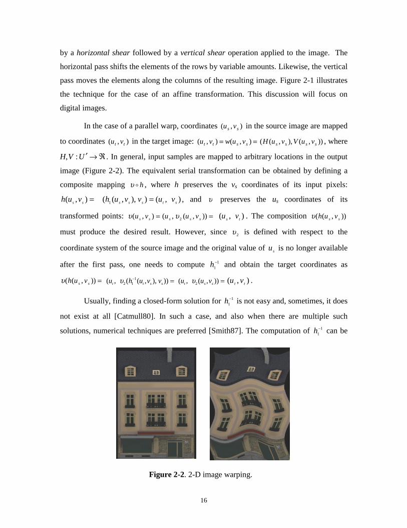
Figure 2-2: 2-D image warping…………………………………………………. ........ 16

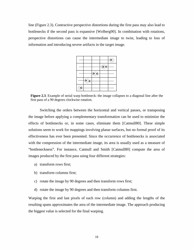
Figure 2-3: Example of serial warp bottleneck. .….……………………………. ........ 18

Figure 2-4: Source image and its view in perspective. .….……………………........... 19

Figure 2-5: Source range image. …………………………………….………….......... 19

Figure 2-6: Result of horizontal-first pass gets twisted (sketch). ………………. ........ 20

Figure 2-7: Result of horizontal-first pass gets twisted (example). …………….......... 20

Figure 2-8: Result of vertical-first pass gets twisted (sketch) …………………. ......... 21

Figure 2-9: Result of vertical-first pass gets twisted (example) ………………. .......... 21

Figure 2-10: Result of parallel war…………….……………….………………. ........... 21

Figure 2-11: Source image rotated by 90 degrees in the same direction of thetransformation before applying a serial warp. …………………………... 22

Figure 2-12: Source image rotated by 90 degrees in the opposite direction of thetransformation before applying a serial warp.….………………………. . 22

Figure 2-13: Perspective view of a brick wall rendered with the relief texture-mappingalgorithm. ……………….……………………………….......................... 23

Figure 2-14: Texture and a surface described by a gray scale image. ………… ............ 23

Figure 2-15: Perspective view of the texture-mapped surface. ………………............... 24

Figure 2-16: Foldover artifact caused by a 2-pass warp. ……………….…….. ............. 24

Figure 2-17: Perspective view of the texture-mapped surface rendered usingrelief texture mapping. ……………….……………….……………..…... 25

Figure 2-18: One-dimensional forward warping and resampling of digital images ……27

Figure 2-19: Texture presenting sharp discontinuities in both horizontal andvertical directions. …..….……………….……………….……………… 28

Figure 2-20: Results of the steps of vertical-first and horizontal-first strategies.. ........... 29

Figure 3-1: Perspective pinhole camera model……………….………………… ........... 32

xviii

Figure 3-2: Parallel projection camera representation. ……………….………… .......... 33

Figure 3-3: Color and depth maps associated with a relief texture…………….............. 33

Figure 3-4: A relief texture and its reprojection viewed from an oblique angle.............. 34

Figure 3-5: Recovering the coordinates of a point in Euclidean space from aperspective image with depth. ……………….……………….…………. 34

Figure 3-6: A point in Euclidean space projected onto both source and targetimage planes. …………………..……….……………….…………….… 35

Figure 3-7: Two-view planar parallax. ……………….…………………………........... 36

Figure 3-8: 2-D schematics for the plane-plus-parallax decomposition. ………. .......... 37

Figure 3-9: Sample sx�

is shifted to ix�

in order to match the view of x� from tC� ............ 40

Figure 3-10: 3-D image warping is equivalent to a pre-warp of the source imagefollowed by conventional texture mapping. …………………………..… 41

Figure 3-11: The pre-warp does not depend on the target image plane…………........... 42

Figure 3-12: Configuration involving two perspective cameras leading tosimplified pre-warping equations. ……………….……………………….43

Figure 3-13: Computing the projection of point x� into a perspective targetcamera from its coordinates in a parallel projection sourcecamera…………………………………………………………………..... 44

Figure 3-14: Parallel and perspective projection cameras sharing the sameimage plane……………….……………….……………………………... 45

Figure 3-15: Line parallel to a plane. ……………….……………….…………. ........... 47

Figure 3-16: Intersection between planes………………….……………….…… .......... 47

Figure 3-17: Top view of a relief texture with point x� projecting at column iu as

observed from C� .……………….……………….……………………... .. 48

Figure 3-18: Another geometric interpretation for the amount of pre-warp shift. …….. 50

Figure 3-19: 2-D view of a scene showing a source camera and target COP….. ............ 52

Figure 3-20: Occlusion-compatible order. ……………….……………….…… ............ 54

Figure 3-21: Occlusion-compatible order: geometric intuition. ………………. ............ 55

Figure 3-22: Pinhole camera model: epipole switches sides. ………………… ............. 56

Figure 3-23: Occlusion-compatible order for parallel projection images…….. .............. 56

Figure 3-24: Occlusion-compatible order for parallel projection images:geometric intuition. …………………….……………….……………….. 57

Figure 3-25: Cell with six perspective projection images…….………………............... 58

Figure 3-26: 2-D representation of a target view inside a cell. ………………. .............. 59

Figure 3-27: 256x256-texel color and depth maps. ……………….………….. ............. 59

xix

Figure 3-28: Three views of a relief texture-mapped brick wall. …………….. ............. 60

Figure 4-1: Structure of the two-pass 1-D relief texture mapping algorithm….. ............ 63

Figure 4-2: Pseudocode for left-to-right warp and resampling of one texel…… ............ 64

Figure 4-3: Warping of one texel. ……………….……………….……………. ............ 65

Figure 4-4: Image created with the two-pass 1-D warping and resamplingalgorithm. ……………….……………….……………….…………….... 66

Figure 4-5: Oblique view of a surface. ……………….……………….……….............. 67

Figure 4-6: Potential self-occlusion. ……………….……………….………….. ........... 67

Figure 4-7: Two ways to perform a serial warp. ……………….………………. ........... 68

Figure 4-8: Serial warp and reconstruction: an example.………………………. ........... 69

Figure 4-9: Graph of Equation (4-2). ……………….……………….…………. ........... 70

Figure 4-10: Texture and depth map associated with a relief texture of aquadrilateral with a deep box at the center. …………………………..… . 71

Figure 4-11: Stages of the pre-warped texture……………….…………………. ........... 71

Figure 4-12: Pseudocode for a first-pass left-to-right horizontal asymmetricwarp and resampling of one texel. ……………….……………………... . 72

Figure 4-13: Reconstruction created with the two-pass asymmetric algorithm…........... 73

Figure 4-14: Stages of the relief texture-mapping algorithm. ……………….………… 73

Figure 4-15: Pseudocode for a first-pass left-to-right horizontal warp withdisplacement compensation. ……………….…………………………... .. 75

Figure 4-16: Correctly computed values……….…….................................................... 76

Figure 4-17: Pipelined reconstruction. ……………….……………….………... ........... 76

Figure 4-18: Pseudocode for left-to-right top-to-bottom warp and resamplingof one texel. ……………….………………………….…………….…… 77

Figure 4-19: Façade of a building warped and resampled using the pipelinedalgorithm. ……………….……………….…………….……………….... 77

Figure 4-20: Mesh-based reconstruction. ……………….……………….…….............. 78

Figure 4-21: Pseudocode for mesh-based reconstruction using OpenGL trianglestrips……………….……………….……………….…………………..... 78

Figure 4-22: Image associated with a relief texture of the front of a statue……............. 79

Figure 4-23: Code fragments used to initialize and use lookup tables in thecomputation of the pre-warped coordinates. ………………………….. ... 80

Figure 4-24: Two views of an object rendered using quantized displacementvalues……………….……………….……………….…………..……. .... 81

Figure 4-25: The changing field of view effect……………….………………… .......... 83

xx

Figure 4-26: Final views (left) and associated pre-warped images. ……………............ 84

Figure 4-27: Actual target field of view. ……………….……………….………........... 86

Figure 4-28: Normalized device coordinates of the vertices of the source imageplane. ……………….……………….……………….……….………...... 86

Figure 4-29: Sharp color discontinuities matched by color change. ………….… .......... 87

Figure 5-1: A relief texture mapped onto two polygons with different sizes andorientations. ……………….……………….………………….……….. .. 90

Figure 5-2: Reprojection of a building façade……………….…………………. ........... 91

Figure 5-3: Light Field representation consisting of a single light slab. ………............. 92

Figure 5-4: Stanford dragon. ……………….……………….……………….… ............ 92

Figure 5-5: An extra quadrilateral is used to map outliers. ………………..…… .......... 93

Figure 5-6: Object represented by six relief textures……………….…………... ........... 93

Figure 5-7: Division of the object space into numbered regions. ………………. .......... 94

Figure 5-8: Pseudocode for rendering object representations. …………………............ 94

Figure 5-9: Displacement versus column values……………….……………….. .......... 95

Figure 5-10: Images associated with four of the six relief textures used torepresent the statue……………….…………………………………….. .. 95

Figure 5-11: Reconstructed view of the statue obtained by texture mappingtwo quads. ……………….……………….……………….…….………. . 96

Figure 5-12: Pre-warped images……………….……………….……………….. .......... 96

Figure 5-13: Another view of the statue rendered with relief textures. ………..... ......... 97

Figure 5-14: Rendering relief textures as continuous surfaces may lead to theoccurrence of “skins”. ……………….……………….………………...... 97

Figure 5-15: Four of the six relief textures used to model a rat………………... ............ 98

Figure 5-16: Skin detection. ……………….……………….……………….… ............. 98

Figure 5-17: Skin-free rendering……………….……………….………………............ 98

Figure 5-18: Occlusion errors. ……………….……………….………………… .......... 99

Figure 5-19: Perceived depth. ……………….……………….………………… ......... 100

Figure 5-20: Relief textures rendered with 8-bit z-correction. ………………… ......... 101

Figure 5-21: Relief textures rendered with z-correction using 8-bit quantizedvalues. ……………….……………….……………………….……….. . 102

Figure 5-22: Scene rendered using a combination of relief texture mapping andconventional techniques. ……………….…………..………………..…. 103

Figure 5-23: Sitterson Hall’s reading room (partial model). ……………….…............ 104

Figure 5-24: Relief textures used in the reading room representation. ………... .......... 104

xxi

Figure 5-25: Modeling of an immersive environment…………………………. .......... 105

Figure 5-26: Reading room rendered using relief texture mapping. …………... .......... 105

Figure 5-27: Northern Vancouver rendered using a mosaic of 5 by 5 relieftextures. ……………….……………….……………….………............. 107

Figure 5-28: Close-up of one of the relief textures used to create Figure 5-27… ......... 108

Figure 5-29: Three views of a surface scanned with UNC nanoManipulator…............ 108

Figure 5-30: Relief textures created locally and sent to remote sites for visualizationfrom arbitrary viewpoints. ……………….……………. ......................... 109

Figure 6-1: Relief texture pyramid. ……………….……………….…………............. 111

Figure 6-2: Image-based LODs. ……………….……………….……………….......... 113

Figure 6-3: Textured LOD produced with 128x128-texel relief textures………. ......... 113

Figure 6-4: Views of a texture LOD rendered from different distances……….. .......... 114

Figure 6-5: A distant object rendered using textured LODs…………………… .......... 114

Figure 6-6: Bilinear versus trilinear resampling. ……………………………… .......... 114

Figure 6-7: Façade observed from a grazing angle. …………………………… .......... 115

Figure 6-8: Relief texture mapping using bilinear and trilinear resampling…… .......... 116

Figure 6-9: Mip-mapped relief texture mapping. ……………………………….......... 116

Figure 6-10: Many-to-one mapping. …………………………………………… ......... 117

Figure 6-11: Inverse pre-warper. ………………………………………………........... 118

Figure 6-12: One-dimensional clipping. ……………………………………..… ......... 120

Figure 6-13: Skin-related artifact. ……………………………………………… ......... 123

Figure 6-14: Cause of the skin-related artifact…………………………………........... 123

xxii

This page left blank intentionally.

xxiii

LIST OF EQUATIONS

Equation 3-1: 3-D image warping equation…………………………. ......... …..……. 35

Equation 3-7: Pre-warping statement for perspective projection images …. ......... …. 40

Equation 3-8: Pre-warping equations for perspective projection images …. ......... …. 40

Equation 3-12: Pre-warping statement for relief textures…………………..… ............. 45

Equation 3-13: Pre-warping equations for relief textures………………… ................... 45

Equation 4-9: Pre-warping equations for relief textures with field of view

compensation ………………………………………..…….................. 86

Equation 5-1: Camera space Z values for samples of a relief texture ……............. … 99

Equation 6-3: One-dimensional clipping……………….………………… .......... … 120

xxiv

This page left blank intentionally.

Chapter 1 – INTRODUCTION

Texture mapping has long been one of the most successful techniques in high-

quality image synthesis [Catmull74]. It can be used to change the appearance of surfaces

in a variety of ways by mapping color, adding specular reflection (environment maps

[Blinn76]), causing vector normal perturbation (bump mapping [Blinn78]) and adding

surface displacements [Cook84], among others. While its meaning can be very broad, the

expression texture mapping will be reserved to refer to its most common use, the

mapping of surface color. Mapping of other attributes, such as bumps and displacements,

will be referred to explicitly.

By adding 2-D details to object surfaces, conventional texture mapping can be

used to correctly simulate a picture on a wall or the label on a can. The planar-projective

transform of texture mapping has a very convenient inverse formulation, which allows

direct computation of texture element coordinates from screen coordinates, leading to

efficient implementation as well as accurate resampling. Unfortunately, texture mapping

Figure 1-1. Town rendered using conventional texture mapping. Each façade and brick wall isrepresented by a single texture.

2

is not as effective for adding 3-D details to surfaces. Its fundamental limitation, the lack

of view-motion parallax1, causes a moving observer to perceive the underlying surface as

locally flat. Such flatness also becomes evident when the surface is observed from an

oblique angle (Figure 1-1).

The most popular approaches for representing surface details are bump mapping

[Blinn78] and displacement mapping [Cook84]. Bump mapping simulates the appearance

of wrinkled surfaces by performing small perturbations on the direction of the surfaces’

normals. It produces very realistic effects, but the technique assumes that the heights of

the bumps are negligibly small when compared to the extent of the associated surface and

it needs to be used in conjunction with per-pixel lighting. Since the surface itself is not

modified, silhouette edges appear unchanged and self-occlusions, which would be caused

by real bumps, are ignored. Surface displacements or displacement maps [Cook84]

specify the amounts by which a desired surface locally deviates from a smooth surface. In

this case, the geometry is actually changed and often rendered as a mesh of micro-

polygons. Displacement maps can be used to create faithful representations for

continuous surfaces, but the associated rendering cost has prevented them from being

used in interactive applications.

This dissertation introduces an extension to texture mapping that supports the

representation of three-dimensional surface detail and view-motion parallax. This new

approach, called relief texture mapping, results from a factorization of the 3-D image

warping equation of McMillan and Bishop [McMillan97] into a pre-warp followed by

conventional texture mapping. The pre-warp is applied to images with per-texel2

displacements, called relief textures, transforming them into regular images by handling

only the parallax effects resulting from the direction of view and the displacement of the

texture elements; the subsequent texture-mapping operation handles scaling, rotation, and

the remaining perspective transformation. The sizes of the displacements can vary

arbitrarily and the results produced by the technique are correct for moving or static

observers standing far away or nearby the represented surfaces. Since relief textures

1 The way the view of a scene changes as a result of viewer motion.2 Texture element

3

contain some geometric information about the surfaces they represent, they can be used

as modeling as well as rendering primitives.

The pre-warping step is described by very simple equations and can be

implemented using 1-D image operations along rows and columns, requiring

interpolation between only two adjacent texels at a time. The final texture mapping stage

is efficiently implemented using conventional texture-mapping hardware.

Relief texture mapping significantly increases the expressive power of

conventional texture mapping and drastically reduces the polygonal count required to

model a scene while preserving its realistic look. The results obtained with the use of this

technique are, in most cases, virtually indistinguishable from the rendering of the more

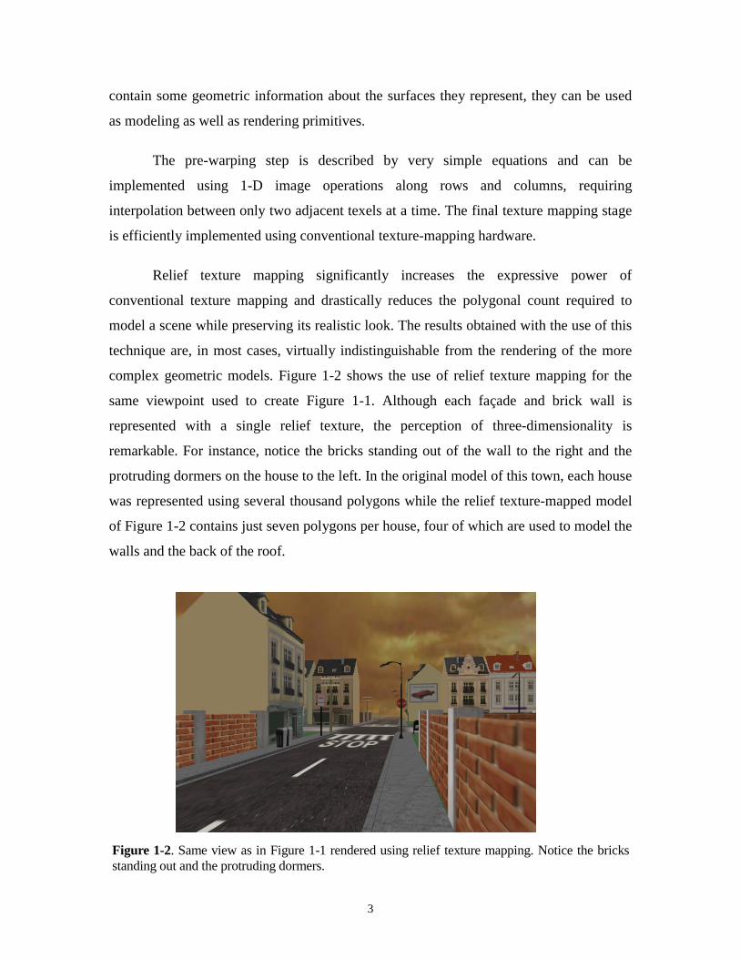
complex geometric models. Figure 1-2 shows the use of relief texture mapping for the

same viewpoint used to create Figure 1-1. Although each façade and brick wall is

represented with a single relief texture, the perception of three-dimensionality is

remarkable. For instance, notice the bricks standing out of the wall to the right and the

protruding dormers on the house to the left. In the original model of this town, each house

was represented using several thousand polygons while the relief texture-mapped model

of Figure 1-2 contains just seven polygons per house, four of which are used to model the

walls and the back of the roof.

Figure 1-2. Same view as in Figure 1-1 rendered using relief texture mapping. Notice the bricksstanding out and the protruding dormers.

4

1.1 Hybrid Systems

In recent years, image-based modeling and rendering (IBMR) techniques have

gained considerable attention in the graphics community because of their potential to

create very realistic images. One of the major benefits of image-based techniques is the

ability to capture details related to the imperfections of the real world that graphics

researchers still do not know how to model and render [Foley00]. By casting a subset of

IBMR, more specifically, the rendering of height images, as an extension to texture

mapping, this research presents an effective technique to construct hybrid systems that

can offer much of the photo-realistic promise of IBMR while retaining the advantages of

polygonal rendering.

1.2 Thesis Statement

I propose to generate valid views of continuous surfaces representing objects and

scenes by warping images augmented with depth using a series of 1-D warps, and

texture-mapping the results onto planar polygons. As in 3-D image warping

[McMillan97], the correctness of the proposed solution is defined as being consistent

with the projections of the corresponding static three-dimensional models represented in

Euclidean geometry. Like all image-based rendering methods, the proposed approach is

essentially a signal reconstruction solution. The central thesis statement of this research is

presented below:

The expressive power of texture maps can be greatly enhanced if textures are

augmented with height fields. Such extended texture maps can be pre-warped

and then conventionally texture-mapped to produce correct perspective views

of surfaces for viewpoints that are static or moving, far away or nearby.

Moreover, the pre-warping step can be implemented using only 1-D image

operations along rows and columns.

Four central issues must be addressed in order to explore the domain associated

with the proposed technique. The first one is the factorization of the 3-D image warping

equation [McMillan97] into pre-warping and texture mapping (a 2-D projective mapping)

5

stages. Chapter 3 presents a derivation of the so-called pre-warping equations. Such

equations can be applied to arbitrary source and target camera configurations. The only

assumption is that the target view is a perspective projection image. I consider parallel

projection images to have some advantages over their perspective projection counterparts

when images are used as modeling primitives. For this reason, pre-warping equations for

both perspective and parallel projection images with depth are derived. Establishing the

visibility of the original samples from arbitrary viewpoints is addressed with an

adaptation of the occlusion-compatible order algorithm [McMillan97] for parallel

projection images.

The second problem involves the reconstruction of a continuous signal from a

discrete input. It also deals with filtering and sampling at the regular lattice of the output

image. Given the special 1-D nature of the pre-warping equations, the resampling process

can be performed in 1-D. This is the subject of Chapter 4, where some resampling

alternatives are explored.

The third issue is the representation and visualization of complex shapes and

objects. The ability to replace complicated shapes with just a few texture-mapped

polygons is an important problem in geometric simplification. This topic is discussed in

Chapter 5, where an algorithm for rendering objects is presented. The increasing interest

for IBMR techniques has popularized the rendering of scenes from images acquired from

real environments. Thus, another important aspect to be considered is the representation

and rendering of such environments using relief texture mapping. This issue is also

discussed in Chapter 5.

The fourth problem is concerned with the use of multi-scale representations of

relief textures. Multi-scale representations in the form of texture pyramids can be used for

anti-aliasing as well as to keep the rendering cost of relief textures proportional to their

contribution to the final image. This subject, as well as shading of relief texture-mapped

surfaces, is discussed in Chapter 6.

6

1.3 Results

This dissertation presents some original results that include:

• an extension to conventional texture mapping that supports the representation

of 3-D surface detail and view-motion parallax,

• a factorization of the 3-D image warping equation into a pre-warp followed by

a 2-D projective mapping,

• a derivation of a family of 1-D pre-warping equations for both parallel and

perspective-projection source images with depth,

• a proof for the one-dimensionality of the pre-warping equations,

• a 1-D clipping algorithm to be used during the pre-warp,

• a family of 1-D resampling algorithms,

• an algorithm for rendering objects with complex shapes represented by sets of

relief textures,

• an adaptation of the occlusion-compatible order algorithm of McMillan and

Bishop to parallel projection images with depth,

• a demonstration that the occlusion-compatible order can be decomposed into

two one-dimensional passes,

• multi-scale image representation for use with image-warping,

• algorithms for constructing scenes by assigning reusable relief textures to

arbitrarily positioned and oriented polygons,

• verification that, after rotations have been factored out, 3-D warps reduce to a

two-dimensional problem that can be implemented as a series of 1-D warps,

regardless of the coordinate systems associated with the source and target

image planes. Moreover, such one-dimensional warps do not suffer from the

shortcomings associated with arbitrary serial warps (bottlenecks, foldovers

and images twists), which are discussed in Chapter 2.

In addition to its original results, the following assertions will be demonstrated:

• complex geometric shapes can be modeled and rendered using the techniques

described in this dissertation,

7

• the use of relief texture mapping can dramatically reduce the polygon count of

a scene when compared to conventional geometric modeling techniques,

• the resampling process associated with the proposed method can be

completely done in 1-D and is simpler than the corresponding operations for

general 3-D image warping,

• relief texture mapping can be used in combination with conventional

geometric models to produce complex scenes with visibility issues

appropriately solved. The proposed approach naturally integrates itself with

popular graphics APIs such as OpenGL [Woo97].

Finally, I expect to provide substantial evidence supporting the claim that the 1-D

operations required for pre-warping and reconstruction lend themselves to a natural

digital hardware implementation.

1.4 Overview of the Relief Texture Mapping Algorithm

Relief texture mapping implements view-motion parallax by pre-warping textures

before mapping them onto polygons (Figures 1-3). Images with depth and a target view

are taken as input. The pre-warping step is responsible for solving visibility issues, filling

holes caused by disocclusion events3 using linear interpolation, and computing the non-

3 Exposures of surfaces not represented in the source images.

Figure 1-3. Relief-texture-mapping algorithm. Images with depth and the desired viewpoint aregiven as input to the pre-warping phase responsible for solving visibility and hole filling. Theresulting image is used as input for a conventional texture-mapping operation that will producethe final image.

Solves visibilityHole fillingNon-planar perspective

Planar perspectiveRotation and scalingFinal filtering

Images withdepth

Pre-warping

Targetview

Final viewPre-warped

images Texture mapping

8

planar component of the perspective distortion. The pre-warp is performed in the

coordinate system of the source images and visibility issues are solved with respect to the

target viewpoint. The final view is obtained by conventionally texture mapping the

resulting pre-warped images onto polygons that match the dimensions, position and

orientation of the image planes associated with the input images. The texture mapping

stage of the algorithm implements rotation, scaling, the planar component of the

perspective distortion and the final filtering. During the pre-warp, depth values associated

with source texels can be interpolated and used to achieve correct occlusions in scenes

containing multiple, and possibly interpenetrating, objects. Figure 1-4 provides a simple

2-D example illustrating the steps of the algorithm, which the reader should be able to

relate to the stages of the pipeline shown in Figure 1-3.

1.5 Related Work

The technique described in this dissertation is derived from the 3-D image

warping method presented in Leonard McMillan’s doctoral dissertation [McMillan97].

Due to its central role in this research, 3-D image warping will receive a detailed

discussion in Chapter 3. Other related approaches have been classified according to their

major features and are presented next.

Figure 1-4. 2-D illustration of the steps of the relief texture-mapping algorithm. The pre-warpingsolves visibility issues and fills holes. The resulting image is used as input for the texturemapping operation that produces the final image.

Pre-warping +reconstruction

Texture mapping

Pre-warped image

Final view

Target view plane

Target viewpoint

Image with depth

Target viewpoint Target viewpoint

9

1.5.1 Image warping methods

Sprites with depth [Shade98] enhance the descriptive power of traditional sprites

with out-of-plane displacements per pixel. Such a technique is based on a factorization

usually referred to in the computer vision literature as plane-plus-parallax [Sawhney94].

Given its importance and its close links with the 3-D image warping equation, such a

factorization will also be considered in detail in Chapter 3. The idea behind sprites with

depth is to use a two-step-rendering algorithm to compute the color of pixels in the target

image from pixels in a source image. In the first step, the displacement map associated

with the source image is forward mapped using a 2-D transformation to compute an

intermediate displacement map. In the second pass, each pixel of the desired image is

transformed by a homography (planar perspective projection) and the resulting

coordinates are used to index the displacement map computed in the first pass. The

retrieved displacement values are then multiplied by the epipole4 of the target image and

added to the result of the homography. Such coordinates are used to index the color of the

destination pixels.

Although such an approach may, at first, seem similar to the mine, given that both

methods use images extended with orthogonal5 displacements, it differs in some

fundamental aspects. Sprites with Depth are an approximation to the 3-D image warping

process. They do not take advantage of available hardware and its 2-D image

reconstruction is more involved and prone to artifacts than the ones presented here. Relief

texture mapping, on the other hand, is based on an exact factorization of the 3-D image

warping equation [McMillan97], takes advantage of texture mapping hardware, uses an

efficient image reconstruction strategy and naturally integrates with popular graphics

APIs. In Figure 1-2, relief textures were pre-warped in software and texture-mapped

using OpenGL [Woo97].

4 The projection of one camera’s center of projection onto the image plane of another camera.5 The techniques described in this dissertation can also be used with source perspective projectionimages with depth. This issue will be discussed in Chapter 3.

10

1.5.2 View-dependent texture mapping

View-dependent texture mapping consists of compositing multiple textures based

on the observer’s viewpoint, and mapping them onto polygonal models. In [Debevec96],

a model-based stereo algorithm is used to compute depth maps from pairs of images.

Once a depth map associated with a particular image has been computed, new views can

be re-rendered using several image-based rendering techniques. Debevec, Yu, and

Borshukov [Debevec98] use visibility preprocessing, polygon-view maps, and projective

texture mapping to produce a three-step, view-dependent texture mapping algorithm that

reduces the computational cost and produces smoother blending when compared to the

work described in [Debevec96].

1.5.3 One-dimensional Perspective Projection

Robertson [Robertson87] showed how hidden-point removal and perspective

projection of height images can be performed on rows and columns. His approach

explores the separability of perspective projection into orthogonal components. First, the

image is rotated to align its lower edge with the lower edge of the viewing window. Then,

a horizontal compression is applied to each scanline so that all points that may potentially

occlude each other fall along the same column. 1-D vertical perspective projection is

applied to the columns of the intermediate image in back-to-front order, thus performing

hidden-point removal. Finally, 1-D horizontal perspective projection is applied to the

resulting image, incorporating compensation for the compression performed in the

second step [Robertson87].

1.5.4 Extension for handling visibility

A nailboard [Schaufler97] is a texture-mapped polygon augmented with a small

depth value per texel specifying how much the surface of an object deviates from the

polygon for a specific view. The idea behind nailboards is to take advantage of frame-to-

frame coherence in smooth sequences. Thus, instead of rendering all frames from scratch,

more complex objects are rendered to separate buffers. The contents of such buffers are

used to create partially transparent textured polygons with per-texel deviations from the

11

objects’ surfaces. These sprites are re-used as long as the geometric and photometric

errors remain below a certain threshold [Schaufler97]. An error metric is therefore

required. When a nailboard is rendered, the depth values associated with each texel are

added to the depth of the textured polygon in order to solve visibility among other

nailboards and conventional polygons.

1.6 Discussion

Impostors have been used to improve a system’s frame rate by reducing the

amount of geometry that needs to be rendered. Some of the most common examples of

impostors include the use of texture-mapped polygons [Maciel95] and levels of detail

[Heckbert97]. While the use of conventionally texture-mapped polygons is very effective

in reducing a scene’s polygonal count, they have limited application due the lack of view-

motion parallax. This research presents a new class of dynamic texture-mapped impostors

that are virtually indistinguishable from the geometric models they represent, even when

the viewer is very close.

An interesting property of relief textures is the ability to adjust their rendering

cost to match their contribution to the final image. Thus, for instance, a surface that is far

away from the viewer can be rendered as a conventional texture or using a low-resolution

level of its associated relief texture pyramid. On the other hand, as the viewer approaches

the represented surface (e.g., when the viewer crosses the plane containing the texture-

mapped polygon), the relief texture can be rendered as a mesh of micro-polygons. The

user application can select the most appropriate rendering strategy for each situation.

12

This page left blank intentionally.

13

Chapter 2 – Separable Transformations

The notion of image warping is at the center of this dissertation and of several

other image-based rendering approaches. This chapter provides formal definitions for

important related concepts, such as images and warp maps, which serve as foundations

for this and subsequent chapters. Its main purpose is to discuss the decomposition of two-

dimensional warps into a series of one-dimensional operations and the advantages of

using such 1-D transformations over their 2-D counterparts. The difficulties associated

with the use of 1-D warps (need for an inverse solution, bottlenecks, image twists, and

foldovers) and their main causes are examined. Examples illustrating the robustness of

the relief texture-mapping algorithm with respect to these problems are provided. This

chapter also introduces the concept of an ideal separable transform, i.e., a 1-D warp in

which source image coordinates can be transformed independently from each other. The

chapter ends with a discussion of one-dimensional intensity resampling, its advantages,

limitations, and applicability to 3-D image warping.

2.1 Images and Warp Maps

A continuous image is a map CUi →: , where 2ℜ⊂U is called the support of the

image, and C is a vector space, usually referred to as its color space [Gomes97]. Besides

color, the elements of C may carry information about other image attributes such as

transparency, depth, etc. A digital image CUid′→′: is a sampled version of a

continuous image, where ( ){ }ZjiyjyxixUyxU jiji ∈∆⋅=∆⋅=∈=′ ,;,:, is an orthogonal

uniform lattice, x∆ and y∆ are positive real numbers, and CC ⊂′ is a quantization of C

[Gomes97].

A 2-D warp map 2: ℜ⊂→WUw is a geometric transformation that deforms the

support of an image, thus producing a new one. Usually, its input is referred to as source

14

image while its output is called destination or target image. When w causes no

superposition of points in the target image, the map is called injective and an inverse

transformation UWw →− :1 exists. Although some simple warping filters implement

invertible transformations, such a property does not hold in general. In the digital case,

the warp map 2: ℜ⊂→′ WUwd distorts the input lattice, usually causing its

orthogonality and uniformity to be lost. An inverse warp is defined as

21 : ℜ⊂→′− UWwd , where W ′ is an orthogonal uniform lattice associated with the

target image. It is important to note that the technique usually referred to as 3-D image

warping [McMillan97] is, in fact, a 2-D warp map. Although from a formal standpoint

such a name may be misleading, it will be used here due to its widespread acceptance.

Given a warp map w and real numbers 1>λ and 10 << µ , w is called an

expansion or expanding transformation if ( ) ( ) YXYwXw −≥− λ for all UYX ∈, .

Likewise, w is called a contraction or contracting transformation if

( ) ( ) YXYwXw −≤− µ for all UYX ∈, . A transformation that preserves distances, i.e.,

( ) ( ) YXYwXw −=− for all UYX ∈, , is called an isometry [Gomes97]. A special kind

of isometry is the identity transformation XXw =)( for all UX ∈ . In general, warping

transformations are not pure expansions, contractions or isometries. Very often, some

regions are locally expanded, whereas others are locally contracted or remain unchanged.

These special geometric transformations have particular importance in image warping.

Expanded or magnified regions require some kind of interpolation and are less

susceptible to aliasing artifacts. On the other hand, contracted or minified areas are more

prone to aliasing, requiring appropriated filtering. Regions where distances are preserved

usually require both reconstruction and filtering to account for a possible grid

misalignment between the source and target digital images. When the isometry is the

identity function, the transformation is unnecessary. This last observation can be explored

to achieve considerable speed up in certain cases and will be discussed in Chapter 3.

15

2.2 Parallel and Serial Warps

Catmull and Smith [Catmull80] showed how affine and perspective

transformations onto planar, bilinear and biquadratic patches could be decomposed into

two 1-D transformations (shears) over rows and columns. Later, Smith [Smith87] showed

that texture mapping onto planar quadric and superquadric surfaces, and planar bicubic

and biquadratic image warps are also two-pass transformable. He coined the expressions

parallel warp and serial warp which refer to the original 2-D map and to the composition

of 1-D transforms that accomplishes a similar result, respectively.

Assuming the row pass takes place first, a two-pass serial warp6 is accomplished

6 Some approaches use more than two passes [Paeth90].

Figure 2-1. Two-pass affine transformation: 45 degrees rotation by applying twoshear operations along the rows and columns of the image.

Horizontalshear

Vertical shear

Rotation

16

by a horizontal shear followed by a vertical shear operation applied to the image. The

horizontal pass shifts the elements of the rows by variable amounts. Likewise, the vertical

pass moves the elements along the columns of the resulting image. Figure 2-1 illustrates

the technique for the case of an affine transformation. This discussion will focus on

digital images.

In the case of a parallel warp, coordinates ),( ss vu in the source image are mapped

to coordinates ),( tt vu in the target image: == ),(),( sstt vuwvu )),(),,(( ssss vuVvuH , where

H, ℜ→′UV : . In general, input samples are mapped to arbitrary locations in the output

image (Figure 2-2). The equivalent serial transformation can be obtained by defining a

composite mapping h�υ , where h preserves the vs coordinates of its input pixels:

=),( ss vuh ),()),,(( 1 stsss vuvvuh = , and υ preserves the us coordinates of its

transformed points: =),( ss vuυ =)),(,( 2 sss vuu υ ),( ts vu . The composition )),(( ss vuhυ

must produce the desired result. However, since 2υ is defined with respect to the

coordinate system of the source image and the original value of su is no longer available

after the first pass, one needs to compute 1

1

−h and obtain the target coordinates as

=)),(( ss vuhυ =− ))),,((,( 112 sstt vvuhu υ =)),(,( 2 sst vuu υ ),( tt vu .

Usually, finding a closed-form solution for 1

1

−h is not easy and, sometimes, it does

not exist at all [Catmull80]. In such a case, and also when there are multiple such

solutions, numerical techniques are preferred [Smith87]. The computation of 1

1

−h can be

Figure 2-2. 2-D image warping.

17

avoided if the original coordinates of pixels in the source image are stored in a lookup

table. This idea was originally suggested by Catmull and Smith [Catmull80] and later

explored by Wolberg and Boult [Wolberg89].

The decomposition of a mapping into a series of independent 1-D operations

presents several advantages over the original 2-D transform [Fant86] [Wolberg90]. First,

the resampling problem becomes simpler. Reconstruction, area sampling and filtering can

be efficiently done using only two pixels at a time. Secondly, it lends itself naturally to

digital hardware implementation. Thirdly, the mapping is done in scanline order both in

scanning the input and output images. This leads to efficient data access and considerable

savings in I/O time. Also, “the approach is amenable to stream-processing techniques

such as pipelining and facilitates the design of hardware that works at real-time video

rates” [Wolberg90].

2.3 Difficulties Associated with Serial Warps

The basic idea behind serial warps is to move pixels to their final positions in the

target image by shifting them along rows and then along columns (or vice versa), so that,

at each pass, one of the coordinates assumes its final value. Thus, besides the difficulty of

finding closed-form solutions for 1

1

−h , serial warps suffer from two major problems,

namely bottlenecks and foldovers [Catmull80]. A bottleneck is characterized by the

collapse of the intermediate image into an area much smaller than the final one. This can

happen if the first pass is not a one-to-one mapping (i.e., not injective). When it occurs,

the final image is usually disrupted. Even if the second pass restores its final shape, some

color information has already been lost. A foldover, on the other hand, is characterized by

self-occlusions of non-planar surfaces.

2.3.1 Bottlenecks

The major sources of bottlenecks are image rotations and perspective distortions

[Wolberg90]. For instance, consider rotating an image by 90 degrees using a serial warp

and assume the horizontal pass takes place first. In this case, all pixels along each row get

mapped to the same column, causing the intermediate image to collapse into a diagonal

18

line (Figure 2.3). Contractive perspective distortions during the first pass may also lead to

bottlenecks if the second pass is expansive [Wolberg90]. In combination with rotations,

perspective distortions can cause the intermediate image to twist, leading to loss of

information and introducing severe artifacts in the target image.

Switching the orders between the horizontal and vertical passes, or transposing

the image before applying a complementary transformation can be used to minimize the

effects of bottlenecks or, in some cases, eliminate them [Catmull80]. These simple

solutions seem to work for mappings involving planar surfaces, but no formal proof of its

effectiveness has ever been presented. Since the occurrence of bottlenecks is associated

with the compression of the intermediate image, its area is usually used as a measure of

“bottleneckness”. For instance, Catmull and Smith [Catmull80] compute the area of

images produced by the first pass using four different strategies:

a) transform rows first;

b) transform columns first;

c) rotate the image by 90 degrees and then transform rows first;

d) rotate the image by 90 degrees and then transform columns first.

Warping the first and last pixels of each row (column) and adding the lengths of the

resulting spans approximates the area of the intermediate image. The approach producing

the biggest value is selected for the final warping.

Figure 2.3. Example of serial warp bottleneck: the image collapses to a diagonal line after thefirst pass of a 90 degrees clockwise rotation.

19

Another solution, proposed by Wolberg and Boult [Wolberg89], consists of

performing a full horizontal-first warp of both the source image and its transpose, and

composing the target image with the best pixels from both results. Image transposition is

performed by a 90 degree clockwise rotation in order to avoid the need to reorder pixels

left to right [Wolberg89]. In this approach, the warp is defined by a set of three spatial

lookup tables (for X, Y and Z) provided by the user. The authors acknowledge the fact

that the occurrence of bottlenecks is intimately related to the order in which the 1-D

warps are performed. They claim, however, that the need for a vertical-first strategy can

be avoided by upsampling the lookup tables before performing the vertical pass. In order

to guide the image composition step, the four corners of each transformed pixel are used

to compute a bottleneck measure. The goal is to minimize the angles between the edges

of the transformed quadrilateral and the rectilinear grid of the output image. The function

φθ coscos=b , computed on a per pixel basis for both warped images, is used for this

purpose, where θ expresses the horizontal deviation from the output grid and φ , the

A B

CD

B’C’

A’

D’

Figure 2-4. A source image, indicate by a rectangle (left). The same source image shown inperspective (right).

Figure 2-5. Source range image.

A B

D C

20

vertical deviation. Pixels presenting the least deviation are used to composite the final

image.

In order to make the implications of bottlenecks more concrete, a simple example

is presented next. Figure 2-4 (right) is a perspective view of a rectangle (left). The

vertices of both quadrilaterals are identified by capital letters, evidencing the existence of

a counter-clockwise rotation. Notice in Figure 2-4 (right) that vertex A’ is to the left of B’

(similar to the relationship between A and B), but D’ is to the right of C’ (as opposed to

their counterparts D and C). Likewise, vertex A’ is above D’, but B’ is below C’. Figure

2-5 shows a texture7 to be warped to the polygon shown in Figure 2-4 (right).

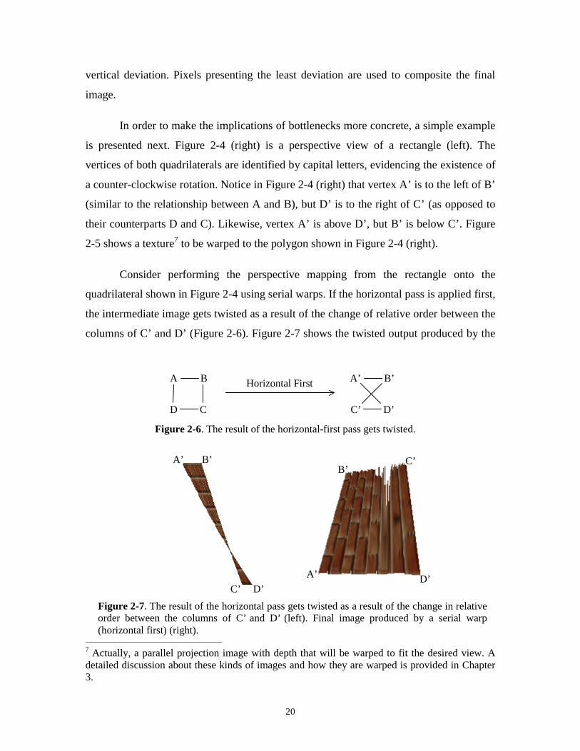
Consider performing the perspective mapping from the rectangle onto the

quadrilateral shown in Figure 2-4 using serial warps. If the horizontal pass is applied first,

the intermediate image gets twisted as a result of the change of relative order between the

columns of C’ and D’ (Figure 2-6). Figure 2-7 shows the twisted output produced by the

7 Actually, a parallel projection image with depth that will be warped to fit the desired view. Adetailed discussion about these kinds of images and how they are warped is provided in Chapter3.

A B

CD

A’ B’

D’C’

Horizontal First

Figure 2-6. The result of the horizontal-first pass gets twisted.

A’

B’C’

D’

B’

C’ D’

A’

Figure 2-7. The result of the horizontal pass gets twisted as a result of the change in relativeorder between the columns of C’ and D’ (left). Final image produced by a serial warp(horizontal first) (right).

21

horizontal warp (left) and the resulting target image (right).

If, however, the vertical pass is executed first, a different twist will introduce

artifacts in the final image (Figure 2-8), brought about this time by the change in the

relative order between the rows with B’ and C’. Figure 2-9 shows the output produced by

the vertical warp (left) as well as the resulting target image (right). Such results should be

compared to the output of a parallel warp (mesh-based reconstruction) for the same view

(Figure 2-10).

Figure 2-9. The result of the vertical pass gets twisted as a result of the change in relative orderbetween the rows with B’ and C’ (left). Final image produced by a serial warp (vertical first)(right).

B’

C’

D’A’

B’C’

D’A’

A B

CD

A’ C’

B’D’

Vertical First

Figure 2-8. The result of the vertical-first pass also gets twisted.

B’C’

D’A’

Figure 2-10. The result of parallel warp (mesh-based reconstruction) to the target image planeis free from the artifacts introduced by serial warps.

22

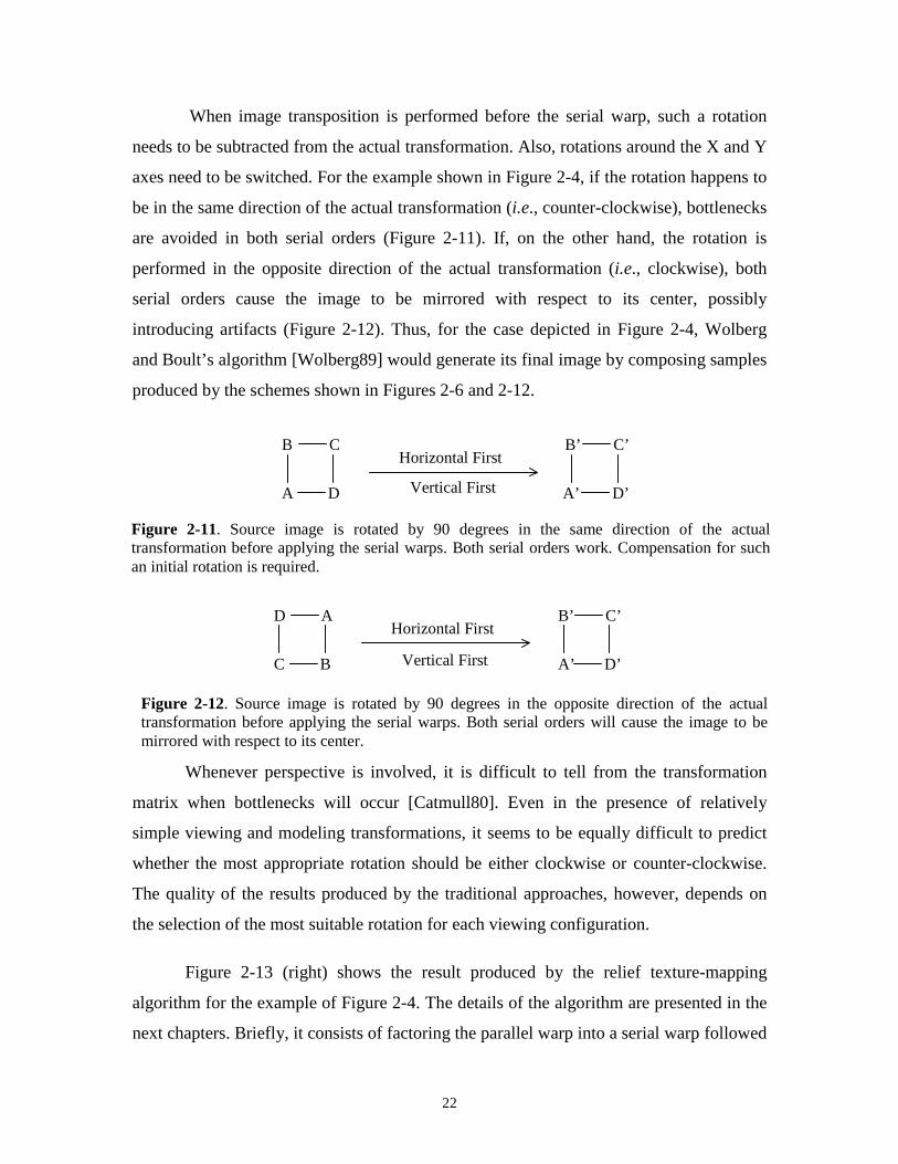
When image transposition is performed before the serial warp, such a rotation

needs to be subtracted from the actual transformation. Also, rotations around the X and Y

axes need to be switched. For the example shown in Figure 2-4, if the rotation happens to

be in the same direction of the actual transformation (i.e., counter-clockwise), bottlenecks

are avoided in both serial orders (Figure 2-11). If, on the other hand, the rotation is

performed in the opposite direction of the actual transformation (i.e., clockwise), both

serial orders cause the image to be mirrored with respect to its center, possibly

introducing artifacts (Figure 2-12). Thus, for the case depicted in Figure 2-4, Wolberg

and Boult’s algorithm [Wolberg89] would generate its final image by composing samples

produced by the schemes shown in Figures 2-6 and 2-12.

Whenever perspective is involved, it is difficult to tell from the transformation

matrix when bottlenecks will occur [Catmull80]. Even in the presence of relatively

simple viewing and modeling transformations, it seems to be equally difficult to predict

whether the most appropriate rotation should be either clockwise or counter-clockwise.

The quality of the results produced by the traditional approaches, however, depends on

the selection of the most suitable rotation for each viewing configuration.

Figure 2-13 (right) shows the result produced by the relief texture-mapping

algorithm for the example of Figure 2-4. The details of the algorithm are presented in the

next chapters. Briefly, it consists of factoring the parallel warp into a serial warp followed

B C

DA

B’ C’

D’A’

Horizontal First

Vertical First

Figure 2-11. Source image is rotated by 90 degrees in the same direction of the actualtransformation before applying the serial warps. Both serial orders work. Compensation for suchan initial rotation is required.

D A

BC

B’ C’

D’A’

Horizontal First

Vertical First

Figure 2-12. Source image is rotated by 90 degrees in the opposite direction of the actualtransformation before applying the serial warps. Both serial orders will cause the image to bemirrored with respect to its center.

23

by conventional texture mapping. Rotations are implemented using the texture mapping

operation and, as a result, the serial warp is free from bottlenecks and image twists.

2.3.2 Foldovers

Foldovers [Catmull80], or self-occlusions, are caused by non-injective 2-D

mappings. Perspective projections of non-planar patches can cause multiple samples to

map to the same pixel on the screen, depending on the viewpoint. If appropriate care is

not taken, samples may be overwritten during the first pass, not being available for the

second one. For example, consider mapping the texture shown on Figure 2-14 (left) onto

the surface described by the gray scale image to its right, where white represents height.

Figure 2-15 shows a perspective view of the resulting texture-mapped surface, which

partially occludes itself. If a vertical-first serial warp is used, some pixels in the upper

central portion of the intermediate image may be overwritten (Figure 2-16 (left)).

Figure 2-14. Texture (left) and a surface described by a gray scale image, where white meansheight (right).

Figure 2-13. Perspective view of a brick wall (right) rendered with the relief texture-mappingalgorithm. Results of the pre-warp: first (horizontal) pass (left); second pass (center).

A’ B’

C’D’ A’

B’C’

D’

A’ B’

C’D’

24

Although they should become visible after the second pass, their information has been

lost and the final image presents some artifacts, as shown by the arrow in Figure 2-16

(right).

The traditional approach for handling self-occlusions in the context of serial

warps is to store both color and depth information in multiple layers. During the second

pass, the depth values are used to perform 1-D warps in back to front order. Catmull and

Smith [Catmull80] suggest the use of multiple frame buffers, one for each fold of the

surface. Such a solution may prove to be too expensive for arbitrary surfaces, which can

potentially present a large number of folds. Wolberg and Boult [Wolberg89] use a more

economic scheme, in which extra layers are allocated on a per column basis. In both

Figure 2-16. Foldover artifact (arrow) caused by a 2-pass warp. Result of the vertical passcause pixels to be overwritten (left). Resulting image (right).

Figure 2-15. Perspective view of the texture-mapped surface obtained after applying the textureshown in Figure 2-14 (left) to the surface shown to its right.

25

cases, appropriate filtering may require accessing multiple layers in order to produce

antialiased output pixels.

Because the warping step of the relief texture-mapping algorithm only deals with

some amount of perspective distortion, it is much less prone to self-occlusions. Figure 2-

17 illustrates the intermediate and final results produced by the algorithm for the example

of Figure 2-15. Nevertheless, a general solution for handling foldovers is presented in

Chapter 4. It consists of interspersing the horizontal and vertical passes and can handle an

arbitrary number of folds without requiring extra storage or depth comparisons.

2.4 The Ideal Separable Transform

The ideal separable transform can be factored as two independent functions of one

variable H, ℜ→′SV : , where { }+ℜ∈∆∈∆⋅=ℜ∈=′ xZixixxS ii ,;: . Thus, =),( tt vu

=),( ss vuw ))(),(( ss vVuH , not requiring the computation of 1

1

−h or the use of lookup

tables. Notice that such a transformation is expected to be faster and scale better than a

regular serial warp. A family of pre-warping equations for relief texture-mapping

satisfying these requirements will be presented in Chapter 3.

Figure 2-17. Perspective view of the texture-mapped surface rendered using relief texturemapping. Results of the vertical (left) and the horizontal pass (center). The final image isshown to the right.

26

2.5 Intensity Resampling

The process of creating new images from discrete ones by means of spatial

transformations is called image resampling. For the case of warped images, it consists of

the following ideal steps [Heckbert89]:

• reconstruct a continuous signal from the input samples

• warp the reconstructed signal

• filter the warped signal to eliminate high frequencies that cannot be captured by

the sampling rate implied by the output grid

• sample the filtered signal to produce the output image.

In practice, a continuous input signal is never actually reconstructed. In fact, only the

significant sample points are evaluated by interpolating the input data. The filtering stage

before the final sampling, however, is still required and is usually referred to as

antialiasing. Nonlinear mappings, such as the ones involving perspective projection,

require the use of adaptive or space variant filters, meaning that the shape and

dimensions of the filter kernel change across the image.

2.5.1 One-dimensional intensity resampling

One-dimensional intensity resampling is considerably simpler than its 2-D

counterpart. 1-D reconstruction reduces to linear interpolation, and antialiasing can be

performed with very little extra computation, by accumulating all contributions to the

currently resampled pixel [Fant86]. Figure 2-18 shows the mapping of an input row onto

an output row. The black segment has slope bigger than one and corresponds to a local

expansion. Dark gray segments have slopes smaller than one and are associated with

local contractions. The light gray segment is a local isometry. A one-dimensional

intensity resampling algorithm can be summarized as follows: if an output pixel falls

completely inside an expanded region, its color is defined by appropriately sampling the

interpolated color at the center of the output pixel. Otherwise, its color is obtained by

weighting the contributions of the various spans covering the pixel. Thus, for instance,

27

the color associated with the fifth pixel in the output row is given by color_at(4.5), where

color_at is a function that returns a linearly interpolated output color for a given

parameter value. Now, let the ut coordinates produced by function H for input pixels 1 to

4 be 0.5, 1.3, 1.7 and 2.4, respectively (Figure 2-18). Since only half of the first pixel in

the output row is actually covered, its color is computed as 0.5*color_at(0.75). Likewise,

the color associated with the second pixel is given by 0.3*color_at(1.15) +

0.4*color_at(1.5) + 0.3*color_at(1.85). In this case, the multiplicative factors represents

pixel coverage by the various spans and the color function is evaluated at the centers of

the span segments covering the pixel.

Suppose that a 2-D antialising process integrates all pixels in a neighborhood N(p) of

a source pixel p to obtain a target pixel p′ . Then, in order for a serial map to perform the

same filtering, all these pixels should be used in the computation of p′ . But this implies

that all pixels in N(p) should map into the same column (row) during the first pass, so that

the second pass can map all their images into p′ [Smith87]. Given that this condition is

seldom satisfied, “it is surprising how often the use of two serial 1-D filtering steps

actually works” [Smith87].

2.5.2 Limitations of one-dimensional serial resampling

Despite the many advantages over parallel warps, the intensity resampling

produced by two-pass methods is not always equivalent to a two-dimensional intensity

Figure 2-18 One-dimensional forward warping and intensity resampling of digital images.Adapted from [Gomes97].

Input row

Output rowlocal expansion

local contraction

0.0

1.0

2.0

3.0

4.0

5.0

6.0

7.0

8.0

1 2 3 4 5 6 7 8

local contraction

local isometry

28

resampling. Although similar for affine transforms, results may vary significantly for

arbitrary warps.

Serial intensity resampling performs poorly when the image resulting from the

first pass presents color discontinuities in the direction of the second pass. Figure 2-19

(left) shows a texture presenting sharp intensity discontinuities in both horizontal and

vertical directions. A simple 2-D warp is defined so that the interior of a squared region is

compressed horizontally and shifted down (Figure 2-19 (right)). Figures 2-20 (a) to (d)

illustrate the outputs of serial resamplings. Figures 2-20 (a) and (b) show the intermediate

and final steps produced by a vertical-first strategy, respectively. Notice that the

horizontal line gets disconnected after the first pass and cannot be recovered by the

second one. The corresponding results produced by a horizontal-first approach are shown

in Figures 2-20 (c) and (d). As the square is horizontally compressed into a rectangle, the

horizontal line maintains its continuity. Notice that although some color discontinuities

were introduced by compressing the vertical line in the central region of the texture, the

resulting artifacts are much less objectionable than the ones in Figure 2-20 (b).

2.6 Discussion

3-D image-warping methods usually map relatively large variations in depth

values into expanded regions, possibly introducing intensity discontinuities not present in

the original texture, such as the one shown in Figure 2-20(a). The magnitude of the

expansions depends on the viewing configuration. The artifacts shown in Figure 2-20 (b)

Figure 2-19. Texture presenting sharp intensity discontinuities in both horizontal and vertical directions(left). A warp defined inside the square region consisting of horizontal compression and vertical shift(right).

29

expose a fundamental limitation of serial resampling methods, and may mistakenly

suggest that the technique is inappropriate for 3-D image-warping applications. In

practice, however, sharp depth discontinuities seem to be associated with smooth color

transitions or, more often, matched by abrupt color variations. None of these cases are

challenges to 1-D reconstruction methods and, for them, the order in which the 1-D

passes are applied (either horizontal or vertical first) seems not to be relevant. This issue

will be discussed in more detail in Chapter 4.

The relief texture-mapping algorithm has several desirable features. First, the

mapping from world to camera coordinate system, perspective transformation, clipping,

hidden surface removal and image resampling are all performed in 1-D. Together, these

operations amount to a significant portion of the whole graphics pipeline. Secondly, as a

scanline algorithm, the approach is suitable for parallel implementation. In each pass, all

rows (columns) can be warped independently from each other. Thus, significant levels of

parallelization can be achieved.

(a) (b)

(c) (d)

Figure 2-20. Results of the passes of a vertical-first strategy: (a) and (b). Results of thepasses of a horizontal-first strategy: (c) and (d).

30

Inverse mapping methods are usually preferred for high-quality image synthesis

applications because filtering naturally fits the construction of the output images. For 1-D

transformations, filtering is extremely simplified and forward mapping produces results

as good as its inverse counterpart. This is extremely important in the context of 3-D

image warping where forward transformations are considerably faster than inverse ones.

31

Chapter 3 – Relief Texture Mapping and the Pre-Warping

Equations

This chapter provides a derivation for a family of ideal separable transforms

called the pre-warping equations and explains their one-dimensional nature. Combined

with texture mapping, such equations can be used to produce correct reprojections of

depth images associated with arbitrary source and target camera configurations.

Particular emphasis is given to the case involving relief textures, which are parallel

projection images with depth, used as modeling and rendering primitives.

The idea behind the relief texture-mapping algorithm is conceptually quite simple:

the 3-D image warp equation [McMillan97] is factored into a serial warp and a

conventional texture mapping operation. Besides performing planar projective

transformations, conventional texture mapping also handles rotations and scaling. Since

the primary sources of difficulties associated with serial warps are image rotations and

perspective distortions, relief texture-mapping benefits from the efficiency of such warps

while avoiding their shortcomings.

3-D image warping [McMillan97] produces correct reprojections of depth images

on arbitrary image planes. Its equation can be factored into a planar perspective

transformation between the source and target image planes, and a per-pixel shift by the

residual planar parallax. If the planar perspective transformation is applied first, the

remaining per-pixel shift needs to handle changes in visibility. If, on the other hand, the

residual shift is applied first, the remaining transformation is not a planar projective

mapping and, therefore, cannot be implemented as a texture mapping operation.

However, the observation that texture mapping is a special case of 3-D image warping

[McMillan97] greatly simplifies the derivation of simple pre-warping equations, since the

problem can be cast as a system involving equations that share many coefficients.

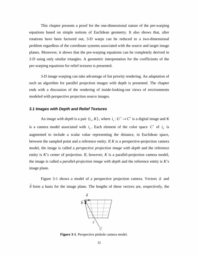
32

This chapter presents a proof for the one-dimensional nature of the pre-warping

equations based on simple notions of Euclidean geometry. It also shows that, after

rotations have been factored out, 3-D warps can be reduced to a two-dimensional

problem regardless of the coordinate systems associated with the source and target image

planes. Moreover, it shows that the pre-warping equations can be completely derived in

2-D using only similar triangles. A geometric interpretation for the coefficients of the

pre-warping equations for relief textures is presented.

3-D image warping can take advantage of list priority rendering. An adaptation of

such an algorithm for parallel projection images with depth is presented. The chapter

ends with a discussion of the rendering of inside-looking-out views of environments

modeled with perspective projection source images.

3.1 Images with Depth and Relief Textures

An image with depth is a pair },{ Kid , where CUid′→′: is a digital image and K

is a camera model associated with di . Each element of the color space C ′ of di is

augmented to include a scalar value representing the distance, in Euclidean space,

between the sampled point and a reference entity. If K is a perspective-projection camera

model, the image is called a perspective projection image with depth and the reference

entity is K’s center of projection. If, however, K is a parallel-projection camera model,

the image is called a parallel-projection image with depth and the reference entity is K’s

image plane.

Figure 3-1 shows a model of a perspective projection camera. Vectors a�

and

b�

form a basis for the image plane. The lengths of these vectors are, respectively, the

Figure 3-1. Perspective pinhole camera model.

c�

b�

a�

C�

33

horizontal and vertical sample spacing in Euclidean space. C� is the center of projection

(COP) of the camera, and c�

is a vector from the COP to the origin of the image plane

[McMillan97].

Figure 3-2 shows the model for a parallel-projection camera. Vectors a�

and

b�

have the same definitions as in the perspective case of Figure 3-1. Vector f�

is a unit

vector orthogonal to the plane spanned by a�

and b�

. The tails of all these vectors are at

C� , the origin of the image plane.

Relief textures are parallel projection images with depth, and are used as modeling

and rendering primitives. Figures 3-3 illustrates the color image and depth map

associated with the relief texture shown in Figure 3-4.

Figure 3-3. Color image (left) and depth map (right) associated with a relief texture.Darker regions in the depth map indicate more distant surfaces.

f�

C�

b�

a�

Figure 3-2. Parallel projection camera representation.

34

3.2 3-D image Warping

Three-dimensional image warping [McMillan97] is a geometric transformation

2: ℜ⊂→′ WUw that maps a source image with depth si onto a target image ti . The

geometric content of the scene is represented implicitly by combining depth information

with the camera model associated with the source image. Thus, let x� be a point in

Euclidean space whose projection into the image plane of si has coordinates ),( ss vu .

Using the perspective projection camera model of Figure 3-1, the coordinates of x� can be

expressed as ),()( ssssss vutbvaucCx����� +++= (Figure 3-5), where the scalar =),( sss vut

bvaucCx sss

����� ++− is the ratio between the distances from sC� to x� and from sC� to

Figure 3-5. Recovering the coordinates of a point in Euclidean space from a perspective image

with depth: ),()( ssssss vutbvaucCx����� +++= .

c�

b�

a�

sC�

x�

),( ss vu

Figure 3-4. A relief texture and its reprojection viewed from an oblique angle.

a�C�f

�

b�

35

pixel ),( ss vu , respectively. In matrix notation:

),(),(

1ssssssss

s

kkk

jjj

iii

s vutxPCvutv

u

cba

cba

cba

Cx���� +=

+=

The projection of x� on an arbitrary target image can be obtained by expressing

the coordinates of x� in both camera systems [McMillan97] (Figure 3-6):

),(),( sssssstttttt vutxPCxvutxPC���

�� +==+

)](),([),( 1tssssssttttt CCvutxPPvutx ���� −+= −

)](),([1tsssssstt CCvutxPPx ���

�� −+= − (3-1)

where =� is projective equivalence, i.e., the same except for a scalar multiple. Notice from

Equation (3-1) that arbitrary target views can be obtained from a single source image

without knowledge about the depth associated with pixels from the desired views.

Dividing Equation (3-1) by ),( sss vut and distributing 1−tP gives:

),()(11

ssststsstt vuCCPxPPx ���

� −+= −− (3-2)

where ),(1),( ssssss vutvu =δ is called the generalized disparity of source pixel

),( ss vu [McMillan97]. Equation (3-2), called the 3-D image-warping equation

[McMillan97], provides a more intuitive interpretation of the underlying process: the

target image is obtained by applying a planar perspective transformation (homography8)

8 Essentially, a texture mapping operation.

Figure 3-6. Point x� in Euclidean space projected onto both source and target image planes

tb�

ta�

sC�

sa�

tC�

x�

sb�

tc�

sc�

36

to the source image, and a per-pixel shift proportional to ),( sss vuδ in the direction of the

epipole of the target view. Such a factorization, often referred to as plane-plus-parallax

in the computer vision literature, avoids many of the inherent ambiguities and instabilities

associated with the decomposition of image motion into its rotational and translational

components [Irani97]. It has been used to produce improved solutions for a variety of

problems in computer vision [Sawhney94] [Kumar94] [Irani96] [Irani97] and constitutes

the basis for a related work on Sprites with Depth [Shade98].

The intuition behind this factorization is explained in Figure 3-7. Let x′� be the

intersection of the source ray, passing through the sampled point x� in Euclidean space,

with a reference plane S, and let tx�

and tx ′� be the projections of x� and x′� , respectively,

into the target image plane. If xx ′= �� for all sampled points, the target image can be

obtained simply by a planar perspective projection of S onto the target image plane. In

general, however, not all samples are coplanar and the differences between the

coordinates of tx�

and tx ′� for all such samples define an epipolar field centered at te�

, the

epipole of the target image. This property can be easily verified by noticing that x� , x′� ,

tx�

, tx ′� and te�

are on the same epipolar plane9 (Figure 3-7). The values associated with

the epipolar field, also referred to as residual planar parallax and represented in Equation

(3.2) by the term ),()(1ssstst vuCCP δ�� −− , can be expressed as )))(/()(( tttZ exdZTH

�� −′−

[Irani96] (Figure 3-8). Here, H is the distance from x� to S, Z and ZT are, respectively, the

9 A plane passing through the centers of projection of two cameras. The intersections of suchplanes with each image plane define the so-called epipolar lines.

Figure 3-7. Two-view planar parallax [Sawhney94].

te�

tx ′�

tx�

x�

tC�

x′�S

sC�

37

depths of x� and the target COP with respect to the source camera, and td is the distance

from S to the target COP (Figure 3-8). The negative sign to the left of H in the epipolar

field expression indicates that x� is in front of S. The expression changes sign as x� crosses

S.

3.3 Factoring the 3-D Image-Warping Equation

Both the homography and the residual planar parallax terms involve two-

dimensional transformations. They are coupled in Equation (3-2) and cannot be

independently applied as is. This can be checked after rewriting Equation (3-2) as

+

=

′′′

2

2

2

1

1

1

w

v

u

w

v

u

w

v

u

t

t

t

(3-3)

with

21

21

ww

uuut +

+=

21

21

ww

vvvt +

+=

where [McMillan97]

)()()(1 ttssttssttsss cbcvcbbucbaCBvAuu��������� ×⋅+×⋅+×⋅=++= (3-4a)

)()()(1 ttssttssttsss accvacbuacaGFvEuv��������� ×⋅+×⋅+×⋅=++= (3-4b)

Figure 3-8. 2-D schematics for the plane-plus-parallax decomposition [Irani96].

TZ

tx′�tx�

sC�

x′�

x�

tC�

H

Z

1

reference plane S

target imagesource image

td

38

)()()(1 ttssttssttsss bacvbabubaaKJvIuw��������� ×⋅+×⋅+×⋅=++= (3-4c)

),()()(),(2 sstttsss vucbCCvuDu δδ ���� ×⋅−== (3-4d)

),()()(),(2 sstttsss vuacCCvuHv δδ ���� ×⋅−== (3-4e)

),()()(),(2 sstttsss vubaCCvuLw δδ���� ×⋅−== (3-4f)

If the homography is followed by a shift in the direction of the epipole, this needs

to handle changes in visibility. The residual planar parallax is given by Equations (3-5a)

and (3-5b) and depends on both terms in Equation (3-3).

( )211

2112

1

1

21

21

www

wuwu

w

u

ww

uuuSHIFT +

−=−++= (3-5a)

( )211

2112

1

1

21

21

www

wvwv

w

v

ww

vvvSHIFT +

−=−

++

= (3-5b)

If the shift towards the epipole represented by the last term in Equation (3-3) is

executed first, the expressions for the remaining transformation are obtained from

Equations (3-5a) and (3-5b) simply by switching the subscripts 1 and 2. In this case,

however, the resulting mapping is not a planar projective transformation and cannot be

implemented as a texture-map operation.

It is interesting to note from Equations (3-4a) through (3-4f) that, if ),( sss vuδ has

a constant value for all pixels of the source image, the 3-D image warping reduces to a

texture mapping operation. In particular, if 0),( =sss vuδ the coordinates of the target

pixels are given by equations (3-6a) and (3-6b) [McMillan97].

KJvIu

CBvAu

w

uu

ss

sst ++

++==

1

1 (3-6a)

KJvIu

GFvEu

w

vv

ss

sst ++

++==1

1 (3-6b)

39

3.4 The Ideal Factorization

Equation (3-2) concisely describes the warping process. From a conventional

rendering point-of-view, the mapping expressed by Equation (3-2) should ideally be

factored so as to allow conventional texture mapping to be applied after the shift in the

direction of the epipole. Such an approach is the opposite of the conventional plane-plus-

parallax decomposition [Sawhney94], in the sense that shifts take place prior to the

homography. It offers some advantages. First, it can benefit from texture mapping

hardware to perform the final transformation and filtering. Secondly, the resulting

equations have a very simple 1-D structure that enables the pre-warp to be implemented

using only 1-D image operations along rows and columns, as will be discussed later in

Chapter 4. Since no rotations are involved, the resulting serial warps do not suffer from

the shortcomings associated with arbitrary serial warps and discussed in Section 2.3.

In order to obtain an ideal factorization, one needs to find a warp 2: ℜ⊂→′ QUp

so that the composition 2: ℜ⊂→′ WUpm � , where 2: ℜ⊂→WQm is a standard

texture-mapping transformation, is equivalent to the 3-D image warp 2: ℜ⊂→′ WUw .

w maps samples from a source image with depth onto the image plane of a target

camera. m should map texels from the source image plane onto pixels in the target image

plane as well. Thus, the fundamental issues are that, during the warp, visibility and the

induced distortion be computed with respect to the target center of projection.

Thus, let ),( ii vu = ),( vvuu ss ∆+∆+ be the intermediate coordinates obtained

after shifting the coordinates of the source pixel ),( SS vu by ),( vu ∆∆ . The equivalence

between the composed mapping pm � and w is modeled by Equations (3-7a) and (3-7b).

The correct interpretation of these equations is critical for the understanding of one of the

central ideas of this dissertation. Simply put, Equations (3-7a) and (3-7b) ask the

following question: What coordinates ),( ii vu should the source pixels ),( ss vu have so that

a view of such a flat distorted image on the source image plane from the target COP would

be identical to a 3-D image warp of the source image onto the target image plane? The

process is illustrated in Figures 3-9 and 3-10. Since the warped image is ready to be

texture-mapped onto the source image plane, it can be mapped onto a polygon that

40

matches the dimensions, position and orientation of such a plane. This notion allows

relief textures to be used as modeling primitives and will be discussed in detail in Chapter

5.

),(

),(

ssss

ssss

ii

ii

vuLKJvIu

vuDCBvAu

KJvIu

CBvAu

δδ

++++++

=++++

(3-7a)

),(

),(

ssss

ssss

ii

ii

vuLKJvIu

vuHGFvEu

KJvIu

GFvEu

δδ

++++++

=++++

(3-7b)

The desired warp p is obtained by solving Equations (3-7a) and (3-7b) for iu and

iv :

),())()()(())()()((

),())()()(())()()((

SS

SSSi vuIFEJDELHIBHJFLAIFEJCEKIGBGJFKA

vuGJFKDFLHJCHKGLBuIFEJCEKIGBGJFKAu

δδ

−+−+−+−+−+−−+−+−+−+−+−

=

),())()()(())()()((

),())()()(())()()((

SS

SSSi vuIFEJDELHIBHJFLAIFEJCEKIGBGJFKA

vuEKGIDIHELCGLHKAvIFEJCEKIGBGJFKAv

δδ

−+−+−+−+−+−−+−+−+−+−+−

=

Dividing both numerators and denominators by +−+− )()(( EKIGBGJFKA

))( IFEJC − , produces the simple one-dimensional equations:

),(1

),(

3

1

SS

SSSi vuq

vuquu

δδ

++

= (3-8a)

),(1

),(

3

2

SS

SSSi vuq

vuqvv

δδ

++

= (3-8b)

or

Figure 3-9. Sample sx�

is shifted to ix�

in order to match the view of x� from tC� .

ix�

sx�

tx�

x�

tC�sC�

41

+

=

′′′

3

2

1

),(

1 q

q

q

vuv

u

w

v

u

SSS

S

i

i

i

δ

where 1q , 2q and 3q are constants for a given configuration of source and target cameras

and, together with ),( ss vuδ , determine the amount of change ),( vu ∆∆ in the coordinates

of the source pixels along epipolar lines.

The pre-warping equations (3-8a) and (3-8b) solve visibility and perform some of

the perspective transformation. The texture-mapping step is responsible for the remaining

perspective distortion, as well as for some scaling and rotation (Figure 3-10).

Figure 3-10. 3-D image warping is equivalent to a pre-warp of the source image followed byconventional texture mapping. The borders of the polygon that matches the source image planeare shown in dashed lines.

tC

target view

forward3-D image

warp

source imageand camera

warped image

sC

pre-warp

texturemapping

Source image plane

42

3.5 Simpler Coefficients

The amount of shift ),( vu ∆∆ to be applied to a source texel only depends on the

position of the target COP (and not on any other target camera parameters), on the

position and orientation of the source image plane, and on the distance from the

associated sample to the source image plane (Figure 3-11). Therefore, one can freely

specify the parameters ta�

, tb�

and tc�

, which define a temporary target camera used only

for the purpose of the pre-warp and which usually differs from the virtual camera used

for the visualization of the final scene. By appropriately choosing such parameters, it is

possible to eliminate several of the coefficients in Equations (3-7a) and (3-7b) by forcing

the corresponding scalar triple products shown in Equations (3-4a) to (3-4f) to have the

form )( wvv��� ×⋅ or )( wvw

��� ×⋅ . Such a procedure leads to a drastic simplification of the

expressions used to compute coefficients 1q , 2q and 3q . For instance, the canceling

process can be made very effective by letting st aa�� α= , st bb

��β= and )( tst CCc ��� −= γ , for

non-zero ℜ∈γβα ,, . This is equivalent to making source and target image planes parallel

to each other, with no relative rotation between them, and to putting the source center of

projection at the origin of the target image plane (Figure 3-12 (left)). In such a case,

coefficients B, D, E, H, I and J become zero and Equations (3-8a) and (3-8b) become

Figure 3-11. The amount of shift to be applied by the pre-warp to the coordinates of a sourcepixel does not depend on the target image plane (not shown).

sc�

iusu

x�

sC�

tC�

source image plane

sample

43

),(1

),(

SS

SSS

i

vuK

L

vuAK

CLu

uδ

δ

+

−= (3-9a)

),(1

),(

SS

SSS

i

vuK

L

vuFK

GLu

vδ

δ

+

−= (3-9b)

3.6 Pre-warping Equations for Relief Textures

The use of parallel projection images as modeling primitives presents some

advantages. For instance, the sampling density is constant across the entire image. Also,

one can take advantage of the perpendicular relationship between the sampling rays and

the image plane of a parallel projection image to produce a simple algorithm to render

these image-based representations. The details of such an algorithm are presented in

Chapter 5.

Given a parallel projection source camera, the coordinates of a point x� in

Euclidean space are given by:

Figure 3-12. Left: configuration involving two perspective cameras leading to simplified pre-warping equations. Right: 2-D representation of the configuration on the left.

tC�

tb� ta

�

tc�

sC�

sb� sa

�

sc�

source viewfrustum

target viewfrustum

target imageplane

source imageplane

tc�

tC�

sC�

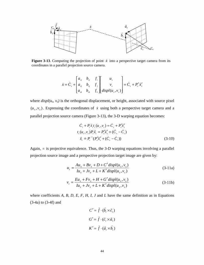
44

sss

ss

s

s

ksksk

jsjsj

isisi

s xPC

vudispl

v

u

fba

fba

fba

Cx ′′+=

+= ����

),(

where displ(us, vs) is the orthogonal displacement, or height, associated with source pixel

),( SS vu . Expressing the coordinates of x� using both a perspective target camera and a

parallel projection source camera (Figure 3-13), the 3-D warping equation becomes:

ssstttttt xPCvutxPC ′′+=+ ���� ),(

)(),( tsssttttt CCxPxPvut ���� −+′′=

))((1

tssstt CCxPPx ����

� −+′′= − (3-10)

Again, =� is projective equivalence. Thus, the 3-D warping equations involving a parallel

projection source image and a perspective projection target image are given by:

),(

),(

ssss

sssst vudisplKLJvIu

vudisplCDBvAuu

′+++′+++

= (3-11a)

),(

),(

ssss

sssst vudisplKLJvIu

vudisplGHFvEuv

′+++′+++

= (3-11b)

where coefficients A, B, D, E, F, H, I, J and L have the same definition as in Equations

(3-4a) to (3-4f) and

)( tt cbfC���

×⋅=′

)( tt acfG���

×⋅=′

)( tt bafK���

×⋅=′

Figure 3-13. Computing the projection of point x� into a perspective target camera from itscoordinates in a parallel projection source camera.

f�

tb�

ta�

Cssa�

Ct

x�

sb�

tc�

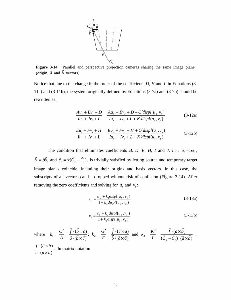
45

Notice that due to the change in the order of the coefficients D, H and L in Equations (3-

11a) and (3-11b), the system originally defined by Equations (3-7a) and (3-7b) should be

rewritten as:

),(

),(

ssss

ssss

ii

ii

vudisplKLJvIu

vudisplCDBvAu

LJvIu

DBvAu

′+++′+++

=++++

(3-12a)

),(

),(

ssss

ssss

ii

ii

vudisplKLJvIu

vudisplGHFvEu

LJvIu

HFvEu

′+++′+++

=++++

(3-12b)

The condition that eliminates coefficients B, D, E, H, I and J, i.e., st aa�� α= ,

st bb��

β= and )( tst CCc ��� −= γ , is trivially satisfied by letting source and temporary target

image planes coincide, including their origins and basis vectors. In this case, the

subscripts of all vectors can be dropped without risk of confusion (Figure 3-14). After

removing the zero coefficients and solving for iu and iv :

),(1

),(

3

1

SS

SSSi vudisplk

vudisplkuu

++

= (3-13a)

),(1

),(

3

2

SS

SSSi vudisplk

vudisplkvv

++

= (3-13b)

where )(

)(1

cba

cbf

A

Ck ���

���

×⋅×⋅=

′= ,

)(

)(2

acb

acf

F

Gk ���

��

×⋅×⋅=

′= and =

×⋅−×⋅=

′=

)()(

)(3

baCC

baf

L

Kk

ts

����

���

)(

)(

bac

baf���

���

×⋅×⋅

. In matrix notation

Figure 3-14. Parallel and perspective projection cameras sharing the same image plane

(origin, a�

and b�

vectors).

tC�

f�

c�

b�

a�

SC�

46

=

′′′′

1

),(

100

0000

010

001

3

2

1

ss

s

s

i

i

i

i

vudispl

v

u

k

k

k

w

z

v

u

Equations (3-13a) and (3-13b) are called the pre-warping equations for relief

textures. The per-texel divisions can be avoided by quantizing the displacement values

(in a pre-processing step) and storing the reciprocal of the denominator of Equation (3-

13a) in a lookup table. This issue will be discussed in Section 4.4.

3.6.1 The one-dimensional nature of the pre-warping equations

Although, at first glance, it may seem surprising that the pre-warping equations

are one-dimensional, the geometric intuition behind this fact is actually very simple and

leads to the computation of even simpler coefficients. It follows directly from the

separability of the perspective projection into orthogonal components. Recall that the pre-

warp simply reprojects a range image with respect to a different center of projection. This

notion of separability into orthogonal components will be explained in the context of

relief textures for the horizontal shift. The same reasoning applies to the vertical case, as

well as to perspective projection images.

Proposition 3-1. Given three planes Π1, Π2 and Π3, so that no two of them are parallel to

each other, if the intersection between Π1 and Π2 is parallel to Π3, then the lines resulting

from the intersections between Π1 and Π3, and between Π2 and Π3 are parallel.

Proof. Let AB be parallel to plane Π3, but not in Π3, and let Π1 be any plane through AB

intersecting Π3 in CD (Figure 3-15). AB and CD cannot meet; otherwise, AB would meet

Π3. Since AB and CD are in Π1, AB and CD are parallel [Euclid]. Now, consider Π2, a

plane through AB intersecting Π3 in EF. Using the same argument, one concludes that

AB and EF are parallel. Since both CD and EF are in Π3, by transitivity, CD and EF are

parallel.

If AB is in Π3, then AB = CD = EF and therefore, CD is parallel to EF.

(q.e.d)

47

Notice that the parallelism between CD and EF is independent of any coordinate

system associated with Π3. In other words, the basis vectors used to span Π3 are not

required to be orthogonal. Thus, let Π3 be an image plane and let AB in Π1 be parallel to

Π3 (i.e., all points in AB are equidistant to Π3), such that the intersection CD between Π1

and Π3 has constant “column” coordinate in the coordinate system associated with Π3

(Figure 3-16). According to Proposition 3-1, each non-empty intersections between Π3

and any plane containing AB is parallel to CD and, therefore, also has constant “column”

coordinate in the coordinate system of Π3. Thus, the intersection between Π3 and the

plane defined by AB and a center of projection C� has constant “column” coordinate in

such a coordinate system. In the context of the pre-warping, such an observation leads to

the following conclusion: for a given camera configuration and displacement/disparity

value, the amount of horizontal (vertical) shift to be applied to a texture element is

independent of its row (column) coordinate. More specifically, the amount of shift only

depends on the position of the target COP, on the position and orientation of the source

C�

A

B

Π3Π1

C

D

Figure 3-16. Intersection CD between Π3 and Π1 has constant “column” coordinate in thecoordinate system of Π3. Π1 contains AB, which is parallel to Π3. The intersection between Π3 and

the plane defined by AB and C� is parallel to CD.

Figure 3-15. AB is parallel to Π3. The intersection of Π3 with plane Π1 passing through AB isparallel to AB [Euclid]. CD and EF are parallel.

Π3

A

B

C

D

Π1

E

F

Π2

48

image plane, and on the distance from the sample to the source image plane. This allows

the computation of the amount of shift to be carried out in two dimensions only and

independently of the coordinate system associated with the image plane.

Figure 3-17 shows a 2-D view of a relief texture observed from C� . The pre-warp

maps point x� , originally at column su , to column iu . Thus, the amount of horizontal

shift applied to the corresponding texel is si uuu −=∆ . By similar triangles (Figure 3-

17):

H

displ

B

u

u

=∆

displH

Bu u=∆ (3-14)

where uB is the distance from eu (the horizontal coordinate of the epipole10) to su :

seu uuB −= (3-15)

Expressing eu in source pixel coordinates

aa

ac

a

acue ��

��

�

��

⋅⋅−=⋅−=

2

H, on the other hand, is given by

displfcH +⋅=��

(3-16)

10 In the case of a parallel projection image, the epipole is obtained by orthographically projectingthe COP of the other camera into the parallel projection image plane.

Figure 3-17. Top view of a relief texture with point x� projecting at column iu as observed

from C� . Triangles C ′ C� x� and su iu x� are similar. eu is the column of the epipole.

a�

eu

c�

f�

C�

iusu

uB

H

displ

x�

C ′

49

The absolute value of u∆ is directly proportional to uB , the horizontal distance

from the epipole to the source texel, and inversely proportional to H, the depth of x� with

respect to C� . The sign of uB , in Equation (3-15), guarantees that the shift is always

towards the epipole. For a given viewing configuration, the amount of horizontal shift

applied to a source texel only depends on its original column and displacement values.

Substituting Equations (3-15) and (3-16) into Equation (3-14) gives

displfc

displuuu se

+⋅−

=∆ ��)(

(3-17)

Computing u∆ directly from the pre-warping equation (3-13a)

ss u

displk

displkuu −

++

=∆3

1

1

displk

displkuku s

3

31

1

)(

+−

=∆ (3-18)

Notice that Equations (3-17) and (3-18) express the same quantity. The former is

obtained after dividing both numerator and denominator of Equation (3-18) by 3k . A

direct inspection of these two expressions reveals that

fck �� ⋅

= 13 (3-19)

and

31 kuk e= (3-20)

It is easy to verify that )(

)(1

bac

baf

fc���

���

�� ×⋅×⋅=

⋅ (see Equation 3-13). Since f

� is a unit

vector perpendicular to the plane spanned by vectors a�

and b�

,

)( baf���

×=α (3-21)where

ba��×

= 1α

Therefore,

50

fcfc

ff

bac

baf����

��

���

���

⋅=

⋅⋅=

×⋅×⋅ 1

)/1(

)/1(

)(

)(

αα

Using similar derivations, the amount of vertical shift can be shown to be

displH

Bv v=∆

where

sev vvB −=and

bb

bcve ��

��

⋅⋅−=

Thus,

displfc

displuvv se

+⋅−

=∆ ��)(

(3-22)

Computing v∆ directly from the pre-warping equation (3-13b)

displk

displkvkv s

3

32

1

)(

+−

=∆ (3-23)

From Equations (3-22) and (3-23), one obtains

32 kvk e= (3-24)

where ev is the row coordinate of the epipole.

Figure 3-18. Another geometric interpretation for the amount of shift applied to point x� as

observed from C� . Triangles x� C ′′ C� and su iu x� are similar. eu is the column of the epipole.

C ′′x�

w

eu

c�

f�

C�

iusu

fck

d��

⋅==3

1

displ

51

3.6.2 Geometric interpretation of the coefficients of the pre-warping equations for

relief textures

Equations (3-19), (3-20) and (3-24) provide a clear geometric interpretation for

the coefficients of the pre-warping equations for relief textures. Figure 3-18 shows the

same situation depicted in Figure 3-17 in terms of the new coefficients. According to

Equations (3-19) and (3-20)

dk

13 = (3-25)

and

d

wkuk e == 31 (3-26)

Thus, 3k is the reciprocal of the distance from the target center of projection ( C� )

to the shared image plane. 1k is the ratio between the horizontal coordinate of the epipole

and the distance from C� to the shared image plane. Likewise, 2k is the ratio between the

vertical coordinate of the epipole and the distance from C� to the shared image plane.

3.6.3 A Useful identity

Proposition 3-2. Given three arbitrary vectors a�

, b�

and c�

in three-space, such that a�

is

not a null vector, the following relationship holds:

aa

cabacbba ��

��������

⋅⋅×−=×⋅×

2

)()(

Proof: From the expressions for 1k , the following equality holds

))(()(

)(3

fcaa

acku

cba

cbfe ����

��

���

���

⋅⋅⋅−==

×⋅×⋅

(3-27)

Substituting Equation (3-21) into the numerator of the left-hand side of Equation (3-27)

and rearranging the terms of the corresponding denominator

))(()(

)()(

fcaa

ac

cba

cbba����

��

���

����

⋅⋅⋅−=

⋅××⋅×α

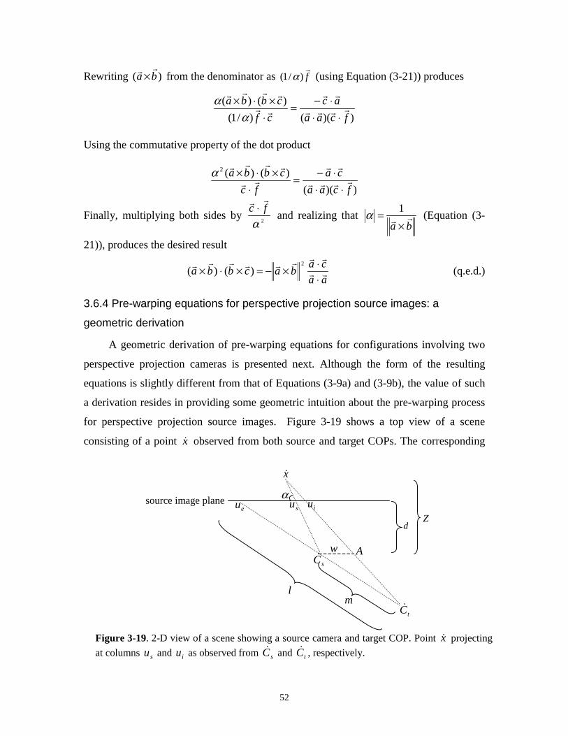
52

Rewriting )( ba��× from the denominator as f

�)/1( α (using Equation (3-21)) produces

))(()/1(

)()(

fcaa

ac

cf

cbba����

��

������

⋅⋅⋅−=

⋅×⋅×

αα

Using the commutative property of the dot product

))((

)()(2

fcaa

ca

fc

cbba����

����

����

⋅⋅⋅−=

⋅×⋅×α

Finally, multiplying both sides by 2αfc�� ⋅

and realizing that ba�� ×

= 1α (Equation (3-

21)), produces the desired result

aa

cabacbba ��

��������

⋅⋅×−=×⋅×

2

)()( (q.e.d.)

3.6.4 Pre-warping equations for perspective projection source images: a

geometric derivation

A geometric derivation of pre-warping equations for configurations involving two

perspective projection cameras is presented next. Although the form of the resulting

equations is slightly different from that of Equations (3-9a) and (3-9b), the value of such

a derivation resides in providing some geometric intuition about the pre-warping process

for perspective projection source images. Figure 3-19 shows a top view of a scene

consisting of a point x� observed from both source and target COPs. The corresponding

Figure 3-19. 2-D view of a scene showing a source camera and target COP. Point x� projecting

at columns su and iu as observed from sC� and tC� , respectively.

α

AwsC�

sueu

tC�

iuZ

d

x�

ml

source image plane

53

projections onto the source image plane are su and iu , respectively. eu is the column

coordinate of the epipole, d is the distance from the source COP to its image plane, and Z

is the depth of x� with respect to sC� . The distances from tC� to sC� and from tC� to eu are

m and l, respectively. According to the definition of generalized disparity [McMillan97],

Zdvu ss /),( =δ .

Triangles is uxu � and AxCs �� are similar and so are triangles ts CAC �� and tie Cuu � .

From the first pair of similar triangles, one has

αα

cos/

cos/)()(

Z

dZ

w

uu si −=−

)),(1()( sssi vuwuu δ−=− (3-28)

Equation (3-28) expresses the amount of horizontal shift applied to source column su .

1),( =ss vuδ when x� is on the image plane, in which case its projection does not move.

As x� switches from one side of the source image plane to another, the sense of the shift

is reversed.

From triangles ts CAC �� and tie Cuu � :

cl

m

uu

w

ei

==− )(

.

Thus,

cuuw ei )( −= . (3-29)

Substituting Equation (3-29) into Equation (3-28) and solving for iu

)1),((1

)1),((

−+−+

=ss

ssesi vuc

vucuuu

δδ

. (3-30)

Using a similar derivation, one obtains

)1),((1

)1),((

−+−+

=ss

ssesi vuc

vucvvv

δδ

. (3-31)

54

3.7 Occlusion-Compatible Order for Parallel Projection Images with Depth

The occlusion-compatible order of McMillan and Bishop [McMillan97], essentially

a painter’s style algorithm, specifies possible orders in which the pixels of a perspective

projection image with depth can be warped, so that correct visibility is achieved for

arbitrary viewpoints without explicit depth comparison. Algorithm 3-1 summarizes the

procedure.

find the projection of the target COP into the source image plane (the epipole);

divide the source image into at most four sheets based on the coordinates of the epipole;

if the target COP is behind the source COP then

for each resulting sheet

warp its samples from the epipole towards the borders of the sheet;

else

for each resulting sheet

warp its samples from the borders of the sheet towards the epipole;

Algorithm 3-1. Occlusion-compatible order for perspective projection source images.

2C�

epipole e12

epipole e21

2a�

2b�

1C�

2c�

1a�

1b�

Figure 3-20. Occlusion-compatible order. The epipole divides the source image in at most foursheets. The arrows indicate the order in which pixels should be warped.

55

Figure 3-20 shows two images playing both source and target image roles. The

white and gray regions represent the sheets when the image acts as source; the arrows

define the warping order. The intuition behind the algorithm is illustrated in Figure 3-21

for the case in which the target center of projection is behind the source COP: whenever

multiple samples fall along a target ray, the one whose corresponding pixel is furthest

from the epipole is the closest to the desired center of projection and, therefore, may

safely overwrite previously warped samples. Thus, source pixels should be warped from

the epipole towards the borders of the image.

In the pinhole camera model, all rays must pass through its COP. This causes the

projection of a point to reverse the side (left/right, top/bottom) of its projection on the

image plane as the point crosses the plane (parallel to the image plane) that contains the

center of projection (Figure 3-22). Thus, although the spatial relationship among the

samples in the source image remains the same, the reference point for the algorithm (the

epipole) may reverse sides as the desired viewpoint moves (Figure 3-22). In such a case,

the order in which the samples are warped needs to be reversed accordingly. This

explains the two possible enumerations of the occlusion-compatible order algorithm. The

COP of a parallel projection image, on the other hand, is at infinity. Thus, the epipole

Figure 3-21. Occlusion-compatible order: geometric intuition. The target center of projection isbehind the source COP. Whenever multiple samples fall along the same target ray, the one whoseprojection into the source image plane is furthest from the epipole is the closest to the target centerof projection.

tC�

sC�

target image plane

epipole

warping direction

target ray

56

does not change as the target COP is moved perpendicularly with respect to the source

image plane (Figure 3-23). Therefore, a single order exists for warping the source pixels.

When parallel projection images with depth are used as source images, samples

falling along a target ray define similar triangles (Figure 3-24). The sides of such

triangles are, respectively, the depth associated with the sample, the distance between the

corresponding pixel and the intersection of the target ray with the source image plane,

and the distance between such an intersection and the sample itself. Due to triangle

similarity, the sample whose corresponding pixel is closest to the epipole is also closest

Figure 3-23. Occlusion-compatible order for parallel projection images. Samples are alwayswarped from the borders towards the epipole.

epipole

sC�

sb�

sa�

tC�

ta�

tb�

tc�

f�

Figure 3-22. Pinhole camera model: the projection of a point changes sides (left/right,top/bottom) in the image plane as the point crosses the plane parallel to the source image planethat contains the COP.

plane containing the COP

source image planeepipole

Source COP

moving target COP

57

to the desired viewpoint (Figure 3-24). Thus, an occlusion-compatible order for parallel

projection images with depth is obtained by always warping pixels from the borders

towards the epipole and is summarized in Algorithm 3-2.

3.7 Pre-Warping Equations for Inside-Looking-Out Cells

Often, texture-mapped impostors are used to replace distant portions of a scene

[Maciel95]. Another commonly used technique to speedup the rendering of large

geometric databases, and particularly suited for indoor environments, consists of

partitioning the space into cells and rendering exclusively the cell containing the current

viewpoint. In this case, only objects that fall inside the current cell need to be rendered as

polygons, while the outside environment is rendered as texture maps. Image warping

Figure 3-24. Occlusion-compatible order for parallel projection images: geometric intuition.Triangles ABC , CBA ′′ and CBA ′′′′ are similar. Similarity of triangles guarantees that anocclusion compatible order is obtained by always warping samples from the borders towards theepipole.

B ′′

C A ′′

B′

A′A

target image plane

tC�

epipolewarping direction

target ray

B

find the projection of the target COP into the source image plane (the epipole);

divide the source image into at most four sheets based on the coordinates of the

epipole;

for each resulting sheet

warp its samples from the borders of the sheet towards the epipole;

Algorithm 3-2. Occlusion-compatible order for parallel projection source images.

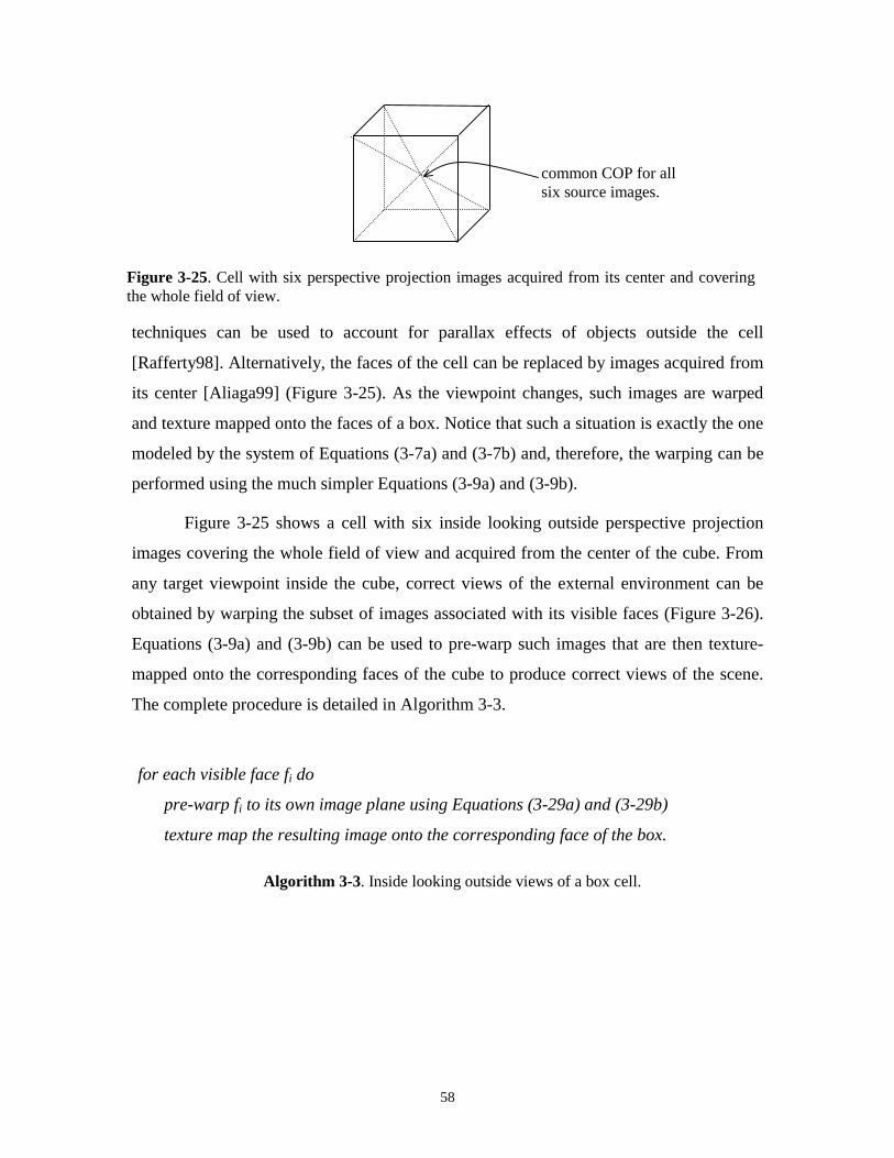
58

techniques can be used to account for parallax effects of objects outside the cell

[Rafferty98]. Alternatively, the faces of the cell can be replaced by images acquired from

its center [Aliaga99] (Figure 3-25). As the viewpoint changes, such images are warped

and texture mapped onto the faces of a box. Notice that such a situation is exactly the one

modeled by the system of Equations (3-7a) and (3-7b) and, therefore, the warping can be

performed using the much simpler Equations (3-9a) and (3-9b).

Figure 3-25 shows a cell with six inside looking outside perspective projection

images covering the whole field of view and acquired from the center of the cube. From

any target viewpoint inside the cube, correct views of the external environment can be

obtained by warping the subset of images associated with its visible faces (Figure 3-26).

Equations (3-9a) and (3-9b) can be used to pre-warp such images that are then texture-

mapped onto the corresponding faces of the cube to produce correct views of the scene.

The complete procedure is detailed in Algorithm 3-3.

for each visible face fi do

pre-warp fi to its own image plane using Equations (3-29a) and (3-29b)

texture map the resulting image onto the corresponding face of the box.

Algorithm 3-3. Inside looking outside views of a box cell.

Figure 3-25. Cell with six perspective projection images acquired from its center and coveringthe whole field of view.

common COP for allsix source images.

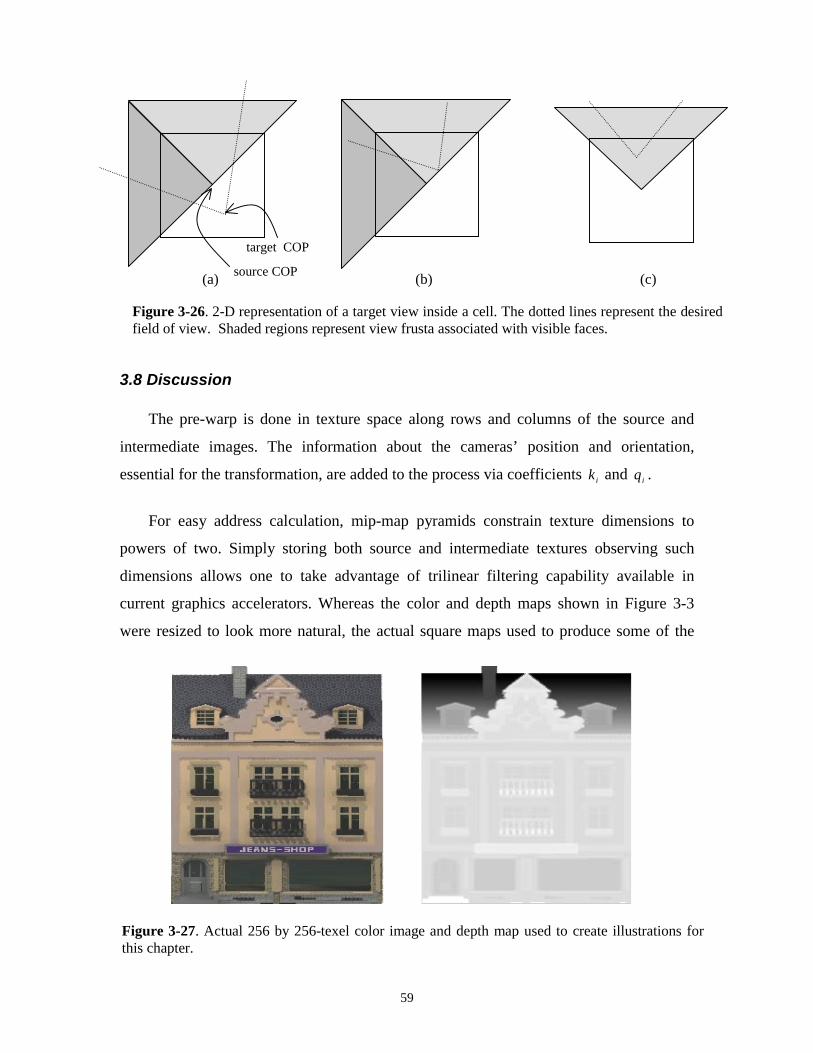
59

3.8 Discussion

The pre-warp is done in texture space along rows and columns of the source and

intermediate images. The information about the cameras’ position and orientation,

essential for the transformation, are added to the process via coefficients ik and iq .

For easy address calculation, mip-map pyramids constrain texture dimensions to

powers of two. Simply storing both source and intermediate textures observing such

dimensions allows one to take advantage of trilinear filtering capability available in

current graphics accelerators. Whereas the color and depth maps shown in Figure 3-3

were resized to look more natural, the actual square maps used to produce some of the

Figure 3-27. Actual 256 by 256-texel color image and depth map used to create illustrations forthis chapter.

Figure 3-26. 2-D representation of a target view inside a cell. The dotted lines represent the desiredfield of view. Shaded regions represent view frusta associated with visible faces.

(a) (b) (c)

target COP

source COP

60

images in this chapter are shown in Figure 3-27. Vectors a�

and b�

associated with the

relief texture are automatically rescaled to compensate for the distortion. In this example,

the rescaling led to higher sampling density along the horizontal dimension (see Figure 3-

4). The resulting pre-warped textures are also square and some scaling is required to

produce correct-looking pictures. This is accomplished automatically by the texture

mapping operation.

Whenever 0),( =ss vudispl (or 0),( =ss vuδ ) then no transformation is necessary.

Figure 3-28 shows multiple views of a relief texture-mapped brick wall. Texels

representing bricks have zero displacement, whereas the mortar is at some depth. The

images on the left correspond to three views of the wall; the ones on the right are the

Figure 3-28. Three views of a relief texture-mapped brick wall. The images on the left showpolygons texture-mapped with the corresponding pre-warped images shown to the right. Bricktexels have zero displacement and, therefore, do not move.

61

associated pre-warped textures. Notice that although the images on the left present

significant visual differences, pixels representing bricks did not move at all in the pre-

warped textures on the right. When a large number of pixels have zero displacement,

such as in the example of Figure 3-28, speed-ups of over 100% were verified in the

current software prototype by just avoiding unnecessary transformations.

62

This page left blank intentionally.

63

Chapter 4 – Image Resampling from Relief Textures

The process of spatially transforming discrete images, usually referred to as image

resampling, is composed of two stages: image reconstruction and a later sampling at the

pixel grid of the output image (section 2.4). Chapter 3 described the warping map, i.e.,

how to determine the coordinates of infinitesimal points in the destination image from

points in the source image. Here, we discuss issues regarding reconstruction, antialiasing

and the final sampling.

The simplest and most common approaches to reconstruction are splatting

[Westover90] and meshing. Splatting requires spreading each input pixel over several

output pixels to assure full coverage and proper interpolation. This usually involves splat-

shape calculation and blending of overlapping samples. Meshing, on the other hand,

requires rasterizing a quadrilateral for each pixel in the NN × input image. The multiple

writes (to possibly incoherent memory positions) of splatting and the setup overhead of

rasterizing tiny quadrilaterals make both approaches very expensive.

The one-dimensional structure of the pre-warping equations allows resampling to

be implemented as a two-pass process using 1-D operations along rows and columns.

Relief texture-mapping algorithm

Figure 4-1. Structure of the two-pass 1-D relief texture-mapping algorithm.

Pre-warp Texture mapping

Horizontal pass Vertical pass

64

Figure 4-1 shows the structure of the two-pass 1-D relief texture-mapping algorithm. The

reader should make a clear distinction between the two steps of the algorithm: pre-

warping followed by texture mapping, and the two phases used to implement the pre-

warp step itself. Such phases consist of a horizontal pass and a vertical pass (Figure 4-1).

The notion of serial resampling is introduced using a simple two-pass strategy.

This is followed by a detailed discussion of the limitations of such an approach and ways

to overcome them. Some filtering issues and the effects of using quantized displacement

values on the quality of the reconstructed images are discussed at the end of the chapter.

4.1 Two-Pass 1-D Resampling

Assume the horizontal pass is completed before beginning the vertical one; either

order is acceptable and either may be advantageous, as discussed in section 2.3. Equation

(3-13a) shows that the pre-warped coordinate iu depends only on its input counterpart Su

and on the input texel displacement. Therefore, each row of the input texture can be

processed independently, with all its texels going to a corresponding row in the

intermediate texture. The elements of each row are processed in occlusion-compatible

order by starting with the element furthest from the epipole and working towards the

epipole. For simplicity’s sake, consider the case when the epipole is to the right and the

warp is proceeding left to right. Figure 4-2 shows a pseudocode for warping one texel

without antialiasing. Antialiasing is implemented using the method described in section

2.5.1. The get and put operations in the pseudocode are reads and writes of the texel at

the indicated index (column, in this case) position. The output element index is computed

based on the input element index and on the displacement of the texel, according to

Figure 4-2. Pseudocode for left-to-right warp and resampling of one texel with coordinateu (or v), index I, color C and displacement D. No antialiasing is treatment is shown forsimplicity.

get Iin, Cin, Din

Inext = Equation_3-13a(Iin,Din)for (Iout = integer(Iprev+1); Iout ≤ Inext; Iout++)

linearly interpolate Cout between Cprev and Cin

linearly interpolate Dout between Dprev and Din

put Cout, Dout at Iout,Iprev=Inext; Cprev=Cin; Dprev=Din

65

Equation (3-13a). The color and displacement values between the previous and current

input texels are linearly interpolated, sampled at each output texel center, and the

sampled values are then stored for use by the next pass. After the horizontal warp has

processed all rows, the same algorithm (replacing Equation (3-13a) with Equation (3-

13b)) is applied to the columns of the resulting image, thus handling the vertical shifts of

texels. Figure 4-3 illustrates the entire process for one texel (B). Figure 4-3(a) shows two

adjacent texels A and B and their positions after the pre-warp (dashed circles). The first texel

of each row is moved to its final column (Figure 4-3(b)) and, as the subsequent texels are

warped, color and displacement values are interpolated during rasterization (Figure 4-3(c)).

Notice that adjacent texels are usually warped to adjacent positions and the situation shown

in Figure 4-3(c) is used to stress the interpolation scheme. This situation may happen, though,

if the adjacent samples are at the boundary of a depth discontinuity. Let texel C be above to

texel B after all rows have been warped (Figure 4-3(d)). During the second pass, the

interpolated displacement values are used to compute the final row coordinates of all texels.

Along columns, each texel is moved to its final row (Figure 4-3(e)) and colors are

interpolated (Figure 4-3(f)).

Figure 4-3. Warping of one texel. (a) Source texels A and B and their final position indicated bydashed circles. (b) The first texel of the current row is moved to its final column. (c) Next texelis moved to its final column and color and displacement values are interpolated duringrasterization. (d) After all rows have been warped, texel C is adjacent to texel B. (e) Verticalpass: row coordinates are computed using the interpolated displacement values and, along eachcolumn, texels are moved to their final rows. (f) Color values are interpolated duringrasterization.

BA

C

(d)

A

(b)(a)

B

A

A

B

BA

(c)

B

A

C

(e) (f)

B

A

C

66

I have compared the results of this simple resampling algorithm to a pre-warp that

uses hardware-based triangular mesh rasterization because the latter is the most common

reconstruction method used in computer graphics. The results are almost

indistinguishable in most cases. The differences are limited to interpolated regions across

depth discontinuities and, therefore, areas not represented in the source images. Figure 4-

4(b) shows a view of a building façade reconstructed using the algorithm. The limitations

of this 1-D resampling strategy are discussed next.

4.1.1 Limitations of the straightforward two-pass 1-D warp

The two-pass algorithm presented in Figure 4-2 is prone to some occlusion and

color interpolation artifacts. Moreover, straight lines may get curved in regions

interpolated across depth discontinuities (Figure 4-5). Whereas the first two kinds of

problems require changes in the resampling strategy, the curved distortion has a simpler

solution.

4.1.1.1 Self-occlusion errors

The straightforward two-pass implementation may, theoretically, cause

information to be lost in the presence of self-occlusions. For instance, consider the

example shown in Figure 4-6. Most of the plane has zero displacement, causing the

Figure 4-4. (a) Color image associated with a relief texture (256x256 texels). (b) View of abuilding generated with the two-pass 1-D warping and resampling algorithm.

(a) (b)

67

corresponding samples to have the same coordinates in both the input and pre-warped

textures. Texels in the diagonal slot are below the plane and should move to the left and

down because the epipole is in the lower left corner. The amount of induced shift during

the horizontal pass may cause some of these texels to be overwritten by others in the

same row. If this happen, the vertical pass has no information about the occluded texels

and thus cannot move them down to the final locations. In Figure 4-6, a pair of dotted

lines represents a hypothetical path associated with a texel and illustrates the problem. In

pratice, however, self-occlusions seem not to introduce noticeable artifacts in the pre-

warped textures. A general solution for this problem, obtained by interspersing the

horizontal and vertical passes, is presented in section 4.2.

Figure 4-6. Potential self-occlusion. The diagonal area corresponds to a deep region, whereasthe rest of the surface has zero displacement. Following a hypothetical path, texel t will moveto the left during the horizontal pass and be overwritten by another texel with zerodisplacement. In this case, no information will be available for the vertical pass.

epipole

texel t

Figure 4-5. Oblique view of a surface. (a) Mesh-based versus (b) two-pass 1-D reconstruction(horizontal pass first). Reconstruction artifacts in (b): straight lines appear curved (left) and wrongcolor interpolation (right) may happen in interpolated regions across depth discontinuities.

(a) (b)

68

4.1.1.2 Color interpolation errors

The two-pass 1-D reconstruction scheme of Figure 4-2 can cause color

interpolation errors across depth discontinuities as shown in Figure 4-5(b). Such artifacts

occur because the pre-warp does not preserve image topology. Thus, consider the four

neighboring pixels A, B, C and D shown in Figure 4-7. In this example, the vertical-first

strategy (Figures 4-7(a), (b) and (c)) produces the same local result as the rasterization of

the corresponding warped quadrilateral. The horizontal-first strategy (Figures 4-7(a), (d)

and (e)), on the other hand, introduces color artifacts. The dashed lines in Figure 4-7(e)

represent improper color interpolation across the boundaries of the warped quadrilateral.

Although such boundaries can be preserved with the use of additional data structures, the

introduction of this extra complexity would diminish some of the advantages resulting

from the simplicity of 1-D warps. In practice, such extra care seems to be unnecessary

most of the time. We will return to this point in the discussion section at the end of this

chapter.

Figure 4-7. Two ways to perform a serial warp: (a) input texels; (b) and (c) results of the stepsproduced by a vertical-first strategy; (d) and (e) results of the steps produced by a horizontal-first strategy. The dashed lines in (e) represent improper color interpolation across theboundaries of the warped quadrilateral ABCD.

(d)

(b)

(a)

A

DC

B W

Y

(e)

(c)

A

DCY

W A

DCY

W

A

DCY

W A

DCY

WB B

B B

69

4.1.1.3 Non-linear distortion

Straight lines may get curved in interpolated regions across depth discontinuities

under the two-pass 1-D algorithm (Figure 4-5(b)). Although no texture information is in

fact available for such expanded areas, the non-linear distortion introduced by the warp

does not correspond to an “expected interpolation behavior”. These artifacts may be

noticed if the expanded regions are relatively large and the texture contains regular

patterns, such as straight lines, across the discontinuities.

The cause of the distortions is the use of a linear fractional transformation11 for

computing the remaining texel coordinate during the second pass. Thus, for instance,

consider a serial warp and reconstruction of the four adjacent texels depicted in Figure 4-

8. The horizontal pass takes place first and the epipole is at the lower right corner. Figure

4-8(b) shows the state immediately after the horizontal pass is concluded. According to

the pseudocode in Figure 4-2, linearly-interpolated values of color and displacements are

sampled and stored at the center of each texel. Although, ideally, performing a serial

warp should be equivalent to performing a parallel warp of the same texels, results may

differ across regions undergoing local expansion. For example, consider texels C and D

in Figure 4-8. Interpolated displacement values are computed for texels labeled 2 and 3

(Figure 4-8(b)) using Equation (4-1).

]1,0[,)()1()( ∈+−= tdispltdisplttdispl DC (4-1)

11 The ratio of two linear functions.

Figure 4-8. Serial warp and reconstruction: (a) source image with four texels highlighted. (b)Intermediate image obtained after the horizontal pass. Interpolated texels are labeled withnumbers. (c) Pre-warped image obtained after the vertical pass.

A B

DC

(a)

A B

DC

1

2 3

(b)

4

2

A

D

C

B1

3

(c)

5 6

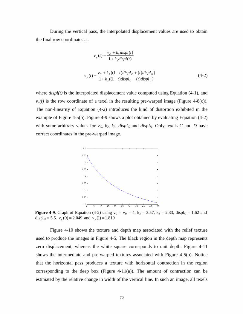
70

During the vertical pass, the interpolated displacement values are used to obtain

the final row coordinates as

)(1

)()(

3

2

tdisplk

tdisplkvtv C

p ++

=

))()1((1

))()1(()(

3

2

DC

DCCp displtdispltk

displtdispltkvtv

+−++−+

= (4-2)

where displ(t) is the interpolated displacement value computed using Equation (4-1), and

vp(t) is the row coordinate of a texel in the resulting pre-warped image (Figure 4-8(c)).

The non-linearity of Equation (4-2) introduces the kind of distortion exhibited in the

example of Figure 4-5(b). Figure 4-9 shows a plot obtained by evaluating Equation (4-2)

with some arbitrary values for vC, k2, k3, displC and displD. Only texels C and D have

correct coordinates in the pre-warped image.

Figure 4-10 shows the texture and depth map associated with the relief texture

used to produce the images in Figure 4-5. The black region in the depth map represents

zero displacement, whereas the white square corresponds to unit depth. Figure 4-11

shows the intermediate and pre-warped textures associated with Figure 4-5(b). Notice

that the horizontal pass produces a texture with horizontal contraction in the region

corresponding to the deep box (Figure 4-11(a)). The amount of contraction can be

estimated by the relative change in width of the vertical line. In such an image, all texels

Figure 4-9. Graph of Equation (4-2) using vC = vD = 4, k2 = 3.57, k3 = 2.33, displC = 1.62 anddisplD = 5.5. 049.2)0( =pv and 819.1)1( =pv

71

are correctly mapped to their final columns. The error is introduced only during the

second pass, as a consequence of the non-linear behavior of Equation (4-2). The

relatively large dimensions of the expanded region (Figure 4-11(b)) allow the distortion

to be noticed.

4.1.2 Correcting the non-linear effects of the interpolation

Several approaches can be used to fix the non-linear distortions introduced by the

straightforward two-pass 1-D reconstruction. All solutions involve some changes in the

computation performed during the first stage of the pre-warp, which will be assumed to

be the horizontal pass. A vertical-first strategy is similar, only involving the renaming of

a few variables.

Let C and D be the previous and current texels under the horizontal pass,

respectively (Figure 4-8). Since serial warps involve three distinct image spaces, namely

Figure 4-11. Stages of the pre-warped texture for the example shown in Figure 4-5(b). Result ofthe horizontal pass (a), and pre-warped image (b).

(a) (b)

Figure 4-10. Texture (a) and depth map (b) associated with a relief texture of a quadrilateralwith a deep box at the center. Black represents zero displacement and white represents deep unitdisplacement.

(a) (b)

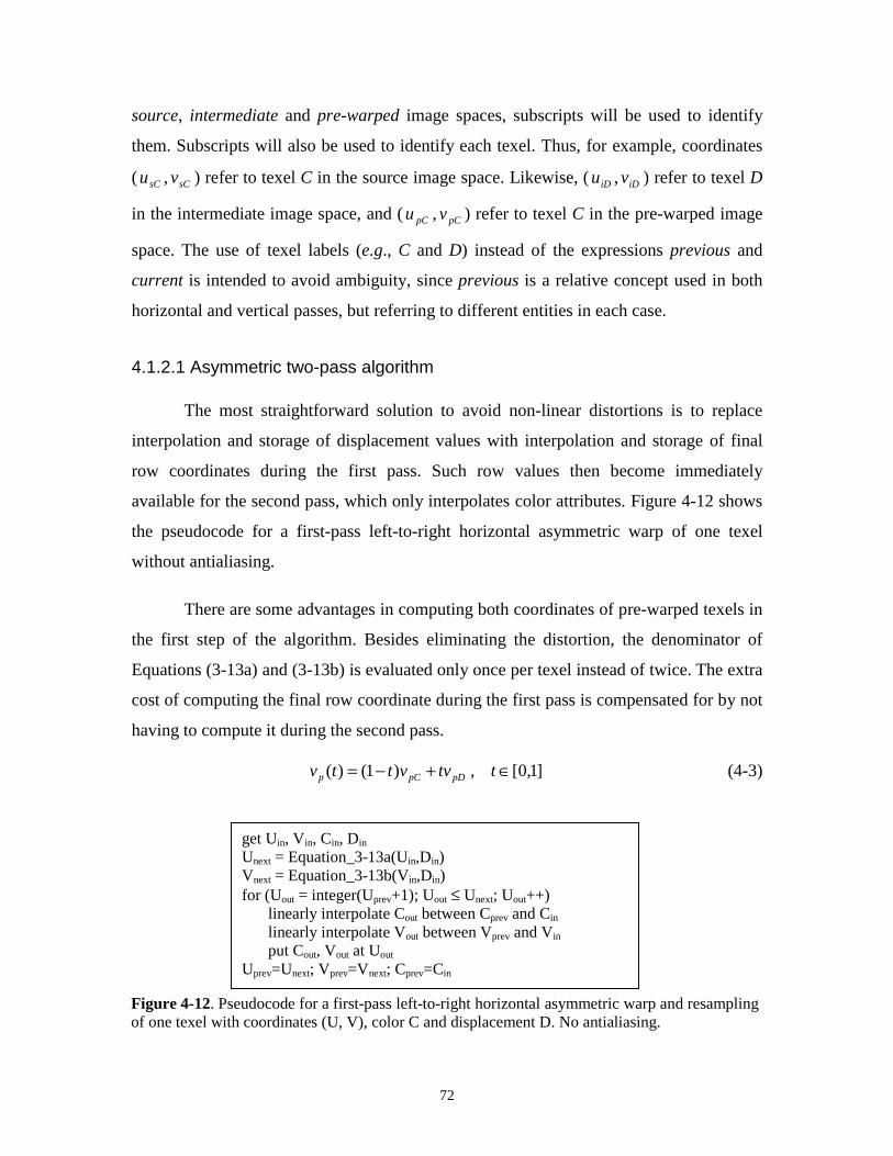
72

source, intermediate and pre-warped image spaces, subscripts will be used to identify

them. Subscripts will also be used to identify each texel. Thus, for example, coordinates

( sCu , sCv ) refer to texel C in the source image space. Likewise, ( iDu , iDv ) refer to texel D

in the intermediate image space, and ( pCu , pCv ) refer to texel C in the pre-warped image

space. The use of texel labels (e.g., C and D) instead of the expressions previous and

current is intended to avoid ambiguity, since previous is a relative concept used in both

horizontal and vertical passes, but referring to different entities in each case.

4.1.2.1 Asymmetric two-pass algorithm

The most straightforward solution to avoid non-linear distortions is to replace

interpolation and storage of displacement values with interpolation and storage of final

row coordinates during the first pass. Such row values then become immediately

available for the second pass, which only interpolates color attributes. Figure 4-12 shows

the pseudocode for a first-pass left-to-right horizontal asymmetric warp of one texel

without antialiasing.

There are some advantages in computing both coordinates of pre-warped texels in

the first step of the algorithm. Besides eliminating the distortion, the denominator of

Equations (3-13a) and (3-13b) is evaluated only once per texel instead of twice. The extra

cost of computing the final row coordinate during the first pass is compensated for by not

having to compute it during the second pass.

]1,0[,)1()( ∈+−= ttvvttv pDpCp (4-3)

Figure 4-12. Pseudocode for a first-pass left-to-right horizontal asymmetric warp and resamplingof one texel with coordinates (U, V), color C and displacement D. No antialiasing.

get Uin, Vin, Cin, Din

Unext = Equation_3-13a(Uin,Din)Vnext = Equation_3-13b(Vin,Din)for (Uout = integer(Uprev+1); Uout ≤ Unext; Uout++)

linearly interpolate Cout between Cprev and Cin

linearly interpolate Vout between Vprev and Vin

put Cout, Vout at Uout

Uprev=Unext; Vprev=Vnext; Cprev=Cin

73

Once the row coordinates of two

Figure 4-13. Reconstruction created with the two-pass asymmetric algorithm. (a) Same view asin Figure 4-5 with curved lines corrected. (b) Corresponding pre-warped texture.

(a) (b)

Figure 4-14. Stages of the relief texture-mapping algorithm created with the asymmetric two-pass approach. (a) Source relief texture. (b) Intermediate image produced by the horizontalpass. (c) Pre-warped texture obtained after the vertical pass. (d) Final view, showing theborders of the texture-mapped polygon.

HorizontalPass

Vertical

TextureMapping

(a) (b)

(c) (d)

74

adjacent texels have been computed, they are linearly interpolated (Equation (4-3)).

Figure 4-13 shows the result obtained with the asymmetric two-pass algorithm for the

surface showed in Figure 4-5. The non-linear distortions have been eliminated. This

asymmetric two-pass algorithm was used to create most of the illustrations shown in this

dissertation and to produce the supporting animations. The use of other reconstruction

strategies is acknowledged explicitly. Figure 4-14 illustrates all stages of the relief

texture-mapping algorithm.

4.1.2.2 Two-pass algorithm with displacement compensation

Alternatively, several approaches can be used to compute corrected displacement

values for the interpolated texels in the first pass so that the desired coordinates are

obtained in the second pass. For instance, substituting the pre-warping equation

D

DsDpD displk

displkvv

3

2

1++

= into Equation (4-3) produces

++

+−=D

DsDpCp displk

displkvtvttv

3

2

1)1()( (4-4)

Equation (4-4) is clearly linear since k3 and Ddispl are both constants, and it can be

rewritten as:

D

DpCpCsDpC

p displk

displtkkvttvvvtv

3

23

1

))1(()()(

++−+−+

= (4-5)

Recall from Equation (4-2) that the interpolated row coordinate of a texel during

the vertical pass is given by:

)(1

)()(

3

2

tdisplk

tdisplkvtv sC

p ++

= (4-6)

The corrected displacement can then be obtained by solving Equations (4-5) and

(4-6) for displ(t):

)(1

)(

1

))1(()(

3

2

3

23

tdisplk

tdisplkv

displk

displtkkvttvvvsC

D

DpCpCsDpC

++

=+

+−+−+

DpCDpCsDDpC

DpCDpCsDpCDsC

displkvtkdisplkvvtkdisplkkv

displkvtdisplkvvtvdisplkvtdispl

2332233

323

)1()()1(

)1()()1()(

−++−++−−−+−−−+

= (4-7)

75

or, more compactly

321

321

)1(

)1()(

γγγβββ

tt

tttdispl

−++−−−

= (4-8)

where

pCDsC vdisplkv −+= )1( 31β

DpCsD displkvv 22 +−=β

DpC displkv 33 =β

2331 )1( kdisplkkv DpC +−=γ

DpCsD displkvv 22 +−=γ

DpC displkv 233 =γ

Notice that most of the terms in these constants can be reused, such as k2displD, k3displD

and (1 + k3displD). The corresponding equations for a vertical-first strategy are obtained

directly from Equations (4-7) by replacing v with u, and k2 with k1.

The corrected displacement values, displ(t), are computed in the first pass using

Equation (4-8) and stored at the interpolated texels. During the second pass, the final row

coordinates are obtained using Equation (4-6). Figure 4-15 shows the pseudocode for a

first-pass left-to-right horizontal warp with displacement compensation. Figure 4-16

shows the result of a simulation for the same parameters used in Figure 4-9 and

superimposed on top of the original graph.

4.2 Pipelined Resampling

The overwriting of texels during the first pass may cause self-occlusions.

Although bottlenecks [Catmull80] are not an issue during the pre-warp step and, in

Figure 4-15. Pseudocode for a first-pass left-to-right horizontal warp with displacementcompensation.

get Uin, Vin, Cin, Din

Unext = Equation_3-13a(Uin,Din)Vnext = Equation_3-13b(Vin,Din)for (Uout = integer(Uprev+1); Uout ≤ Unext; Uout++)

linearly interpolate Cout between Cprev and Cin

Dout = Equation_4-8(Vprev,Vin, Din)put Cout, Dout at Uout,

Uprev=Unext; Vprev=Vnext; Cprev=Cin

76

practice, self-occlusions seem not to introduce noticeable artifacts in the pre-warped

textures, we present a solution that is capable of handling an arbitrary number of

foldovers and that does not require depth comparison. It consists of interspersing the

horizontal and vertical warps. As before, assume the horizontal pass is completed first

and the rows are processed in occlusion-compatible order. As the horizontal warp

produces each intermediate texel, this is immediately interpolated into the appropriate

column. Since each vertical warp receives and processes its texels in occlusion-

compatible order, correct visibility is preserved in the output. Also, because each texel is

processed immediately after its generation, no information is overwritten and self-

occlusions are avoided. The steps of the algorithm are illustrated in Figure 4-17, where

light gray circles represent the texels previously warped to the corresponding columns.

Figure 4-18 presents a pseudocode for the pipelined warp and resampling and Figure 4-

19 shows an image reconstructed with the algorithm.

Parameter t

Figure 4-16. Correctly computed values superimposed on top of the graph of Figure 4-9.

Figure 4-17. Pipelined reconstruction: (a) Two adjacent texels and their final positions after thewarping (dashed circles). (b) Horizontal interpolation. Dashed lines represent linearinterpolation. (c) The new values are vertically interpolated as soon as they become available.

(b)

A B

(c)

A

B

(a)

B

A

B

A

77

4.3 Mesh-Based Resampling

For the cases in which color interpolation errors may become a concern, the 1-D

reconstruction can be replaced with a mesh-based approach. This can be done while still

taking advantage of an occlusion compatible ordering. Thus, consider the situation

depicted in Figure 4-20, in which the epipole splits a relief texture into four sheets. Each

sheet is warped and reconstructed as a set of triangle strips as shown for the first row of

Figure 4-19. Façade of a building warped and resampled using the pipelined algorithm.

Figure 4-18. Pseudocode for left-to-right top-to-bottom pipelined warp and resampling of onetexel with coordinates (U, V), color C and displacement D. C[Uout] and V[Uout] are the color androw coordinates of the last sample warped to column Uout.

get Uin, Vin, Cin, Din

Unext = Equation_3-13a(Uin,Din)Vnext = Equation_3-13b(Vin,Din)for (Uout = integer(Uprev+1); Uout ≤ Unext; Uout++)

linearly interpolate Cout between Cprev and Cin

linearly interpolate Vout between Vprev and Vin

for (Vfinal=integer(V[Uout]+1); Vfinal ≤ Vnext; Vfinal++)linearly interpolate Cfinal between C[Uout] and Cout.put Cfinal at (Uout, Vfinal)

Uprev=Unext; Vprev=Vnext; Cprev=Cin

78

the top left sheet. The arrows specify the order in which pixels from two consecutive

rows should be visited. Notice that the coordinates used for triangle rasterization are the

pre-warped coordinates of the corresponding texels. The resulting 2-D triangles are

rasterized without performing depth comparison. While mesh-based reconstruction is not

subject to nonlinear distortions or color interpolation artifacts, it requires rasterizing

approximately two triangles per each NN × texels of the input texture.

Figure 4-21 presents a pseudocode for mesh-based reconstruction of the top left

sheet that uses OpenGL-like functions to implement the rasterization. This approach was

used to generate the image shown in Figure 4-5(a).

Figure 4-20. Mesh-based reconstruction. Relief texture split into four sheets. The arrowsindicate the order in which texels from consecutive rows of the top left sheet should be visitedto produce triangle strips.

Initialize a reuse buffer with color and warped coordinates for the first sheet rowfor (V = Vinitial +1; V ≤ Vfinal; V++) glBegin(GL_TRIANGLE_STRIP)

for (U = Uinitial; U ≤ Ufinal; U++) glColor(reuse_buffer[U].color) glVertex(reuse_buffer[U].u, reuse_buffer[U].v)

texel.u = Equation_3-13a(U, D[U, V])texel.v = Equation_3-13b(V, D[U, V])

texel.color = color(U, V) glColor(texel.color) glVertex(texel.u, texel.v) reuse_buffer[U] = texel;

glEnd()}

Figure 4-21. Pseudocode for mesh-based reconstruction of the top left sheet using OpenGLtriangle strips. (Uinitial, Vinitial) and (Ufinal, Vfinal) are the coordinates of the top left and bottomright texels of the sheet, respectively. D[U,V] is the displacement value associated with texel(U,V). color(U,V) is the color associated with texel coordinates (U, V).

79

4.4 Reconstruction Using Quantized Displacement Values

As defined in Chapter 3, a relief texture is composed of color, depth and camera

information. The camera data are specified by three vectors ( a�

, b�

and f�

) and a point

( C� ) (Figure 3-2). If the displacement associated with each texel is stored as a float, the

storage requirement for the depth information matches the amount needed for the color

data (32 bits per sample). In this case, transferring a relief texture from main memory to

texture memory would require twice as much bandwidth and space as a regular texture.

Such requirements can be reduced to essentially the same as for regular textures by

storing quantized displacement values in the alpha channel of the relief texture. This

strategy also helps to improve cache coherence, since the displacement and color data

associated with a texel are always used together.

In a pre-processing step, the minimum and maximum displacement values

associated with the relief texture are identified. A quantization step, qs, is then computed

as

−=

254

minmaxqs

and the indices for the quantized values are obtained from the actual displacements using

the formula

−=qs

displqi

minint .

Figure 4-22. Image associated with a relief texture of the front of a statue. The black pixelsrepresenting the background are identified by a reserved depth value and are skipped during thepre-warp.

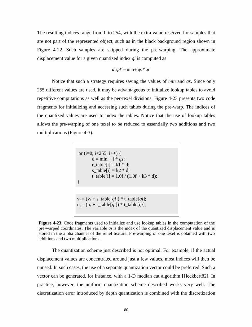
80

The resulting indices range from 0 to 254, with the extra value reserved for samples that

are not part of the represented object, such as in the black background region shown in

Figure 4-22. Such samples are skipped during the pre-warping. The approximate

displacement value for a given quantized index qi is computed as

qiqsldisp *min+=′

Notice that such a strategy requires saving the values of min and qs. Since only

255 different values are used, it may be advantageous to initialize lookup tables to avoid

repetitive computations as well as the per-texel divisions. Figure 4-23 presents two code

fragments for initializing and accessing such tables during the pre-warp. The indices of

the quantized values are used to index the tables. Notice that the use of lookup tables

allows the pre-warping of one texel to be reduced to essentially two additions and two

multiplications (Figure 4-3).

The quantization scheme just described is not optimal. For example, if the actual

displacement values are concentrated around just a few values, most indices will then be

unused. In such cases, the use of a separate quantization vector could be preferred. Such a

vector can be generated, for instance, with a 1-D median cut algorithm [Heckbert82]. In

practice, however, the uniform quantization scheme described works very well. The

discretization error introduced by depth quantization is combined with the discretization

or (i=0; i<255; i++) {d = min + i * qs;r_table[i] = k1 * d;s_table[i] = k2 * d;t_table[i] = 1.0f / (1.0f + k3 * d);

}

vt = (vs + s_table[qi]) * t_table[qi];ut = (us + r_table[qi]) * t_table[qi];

Figure 4-23. Code fragments used to initialize and use lookup tables in the computation of thepre-warped coordinates. The variable qi is the index of the quantized displacement value and isstored in the alpha channel of the relief texture. Pre-warping of one texel is obtained with twoadditions and two multiplications.

81

errors of the source and pre-warped images and undergoes the same filtering process. The

results are virtually indistinguishable from the ones obtained with the use of the actual

displacement values, even for complex shapes. Figure 4-24 shows two views of a statue

rendered with the relief texture-mapping algorithm using quantized displacement values.

Notice the details on the face and hair.

4.5 Rendering Statistics

For a typical 256x256-texel relief texture (e.g., Figure 4-4(a)) mapped onto a

single quadrilateral using the asymmetric two-pass approach, the current software

prototype, written in C++, achieves an average frame rate of 9.42 frames per second.

Such measurements were performed on a Pentium II PC running at 400MHz with an

Intergraph graphics accelerator (Intense 3D RealiZm II VX113A-T) with 16 MB of

texture memory and 16MB of frame buffer memory. The final view of the surface was

displayed on a 512x512-pixel window. The percentage of the rendering time spent with

pre-warping and resampling, loading pre-warped textures into texture memory, and the

actual texture mapping operation are shown in Table 4-1. Notice that since the pre-

warping and resampling operations dominate the rendering time, these results are

essentially independent of the dimensions of the output window.

Figure 4-24. Two views of an object rendered using quantized displacement values. Despitethe geometric complexity, they are essentially indistinguishable from the renderings obtainedusing the actual displacements.

82

Pre-warping andresampling

Loading pre-warpedtextures into texture

memory

Actual texturemapping operation Others

94.10% 2.65% 0.066% 3.18%

The use of quantized displacement values did not significantly reduce the

rendering time in the current prototype. For relief textures of dimension 256x256

containing less than 5% background texels, the average speedup was only about 2%.

Given that the pre-warping and resampling dominates the rendering time, a hardware

implementation of these steps can significantly improve the performance of the entire

algorithm. It can also take better advantage of displacement quantization.

4.6 Filtering Composition

A texture undergoes three resamplings during a relief texture-mapping operation:

two as part of the pre-warp and a latter 2-D resampling as part of the conventional texture

map stage. During the pre-warp, some regions of the image are compressed while others

are expanded, requiring the 1-D filters used for reconstruction to change width along the

rows and columns adaptively. Thus, these 1-D filters are adaptive asymmetric triangle12

filters, and the whole pre-warp reconstruction consists of bilinear interpolation using an

anisotropic adaptive filter. The reconstruction filter used by the relief texture-mapping

algorithm is then obtained by convolving a box filter (used by texture mapping hardware)

with the anisotropic filter used by the pre-warp.

It is important to make a distinction between the separability13 of the warping and

reconstruction filters used by the pre-warp. The first, represented by the pre-warping

equations (3-13a) and (3-13b), is clearly separable. The reconstruction filter, on the other

12 A triangle filter is also known as tent filter, Bartlett filter, Chateau function and roof function.

Table 4-1: Percentage of the average rendering time associated with the steps of therelief texture-mapping algorithm (one relief texture mapped onto one quadrilateral).

83

hand, is not separable in general and causes the color interpolation artifacts discussed in

section 4.1.1.2.

4.7 The Changing Field of View Effect

The three resampling steps mentioned in section 4.5 produce good antialiased

images without introducing excessive blurring. In Section 3-6, in order to simplify the

computation of coefficients 1k , 2k and 3k , the image planes of both the source and the

temporary14 target cameras were identified (Figure 3-14). As a result, the field of view of

the temporary camera varies with the viewer’s position (Figure 4-25). As the viewer

moves away from the source image plane, such a field of view decreases and the

projected area of the represented surfaces increases (Figure 4-25(a)). Likewise, as the

viewer moves towards the source image plane, the field of view increases and the

projected area of the represented surfaces decreases (Figure 4-25(b)). The relationship

between the final view and the pre-warped texture is illustrated in Figure 4-26. The

images shown on the left correspond to the final view of the scene while the images on

the right are the output of the pre-warp process. Figures 4-26(a) and (b) correspond to the

situation represented in Figure 4-25(a). The pre-warped image is minified as a

consequence of the planar perspective distortion, implemented by the texture mapping

13 A filter is said to be separable if it can be decomposed into simpler functions, each of which isindependently applied to distinct dimensions of the input signal.14 Used for the purpose of the pre-warp only. See Section 3.5.

Figure 4-25. The changing field of view effect. The viewer moves with respect to a fixed sourceimage plane causing the field of view of the temporary camera (shaded triangle) to change. The sizeof the projected area of the surfaces varies inversely with the changes in the field of view.

(a)

c�

(b)

c�

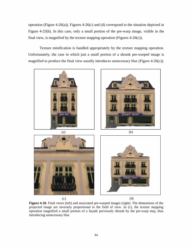
84

operation (Figure 4-26(a)). Figures 4-26(c) and (d) correspond to the situation depicted in

Figure 4-25(b). In this case, only a small portion of the pre-warp image, visible in the

final view, is magnified by the texture mapping operation (Figures 4-26(c)).

Texture minification is handled appropriately by the texture mapping operation.

Unfortunately, the case in which just a small portion of a shrunk pre-warped image is

magnified to produce the final view usually introduces unnecessary blur (Figure 4-26(c)).

(a) (b)

(c) (d)Figure 4-26. Final views (left) and associated pre-warped images (right). The dimensions of theprojected image are inversely proportional to the field of view. In (c), the texture mappingoperation magnified a small portion of a façade previously shrunk by the pre-warp step, thusintroducing unnecessary blur.

85

This situation can be improved by using the full resolution of the pre-warped image to

represent only its visible portion. This is equivalent to clipping the field of view of the

temporary target camera against the field of view of the actual target camera and to

rescaling the temporary a�

and b�

vectors (Figure 4-27). The implementation of these

operations is explained next.

First, the normalized device coordinates (i.e., the coordinates obtained after

perspective projection and division by the homogeneous coordinate w) of the vertices of

the source image plane are computed. By definition, the visible portion of a scene ranges

from [-1, 1] in normalized device coordinates in X and Y dimensions [Foley90]. Figure

4-28 illustrates the situation in 2-D for the X dimension. The new a�

vector is computed

as

amM

a��

+=′ 2

,

where M and m are the absolute values of the maximum and minimum normalized device

coordinates associated with the horizontal limits of the source image plane (Figure 4-28).

The new b�

vector is computed similarly using the plane’s vertical limits. Notice that the

origins of the source image plane and of its visible portion do not coincide in general.

Also, vectors a�

and b�

have been rescaled. Both factors need to be compensated for

during the pre-warp. This will be explained for the column coordinate. The row

coordinate is similar. Thus, let arr be the ratio between the lengths of a�

and a′� , and let

0u be the column coordinate of the origin of the visible portion of the source image plane

expressed in the coordinate system of the source image itself. Recall from Equation (3-

13a) that

),(1

),(

3

1

SS

SSSi vudisplk

vudisplkuu

++

= .

Also recall that )(

)(1

tts

tt

cba

cbfk ���

���

×⋅×⋅

= , )(

)(2

tts

tt

acb

acfk ���

���

×⋅×⋅

= and fc

kt

�� ⋅= 1

3 . Vectors ta�

and tb�

have been rescaled, but since they appear in both numerator and denominator of 2k and

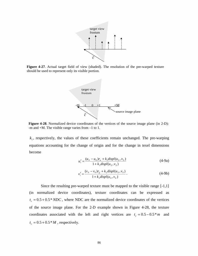
86

1k , respectively, the values of these coefficients remain unchanged. The pre-warping

equations accounting for the change of origin and for the change in texel dimensions

become

),(1

),()(

3

10

SS

SSaSi vudisplk

vudisplkruuu

++−

=′r

(4-9a)

),(1

),()(

3

20

SS

SSbS

i vudisplk

vudisplkrvvv

++−

=′r

. (4-9b)

Since the resulting pre-warped texture must be mapped to the visible range [-1,1]

(in normalized device coordinates), texture coordinates can be expressed as

NDCtc *5.05.0 += , where NDC are the normalized device coordinates of the vertices

of the source image plane. For the 2-D example shown in Figure 4-28, the texture

coordinates associated with the left and right vertices are mtc *5.05.0 −= and

Mtc *5.05.0 += , respectively.

Figure 4-28. Normalized device coordinates of the vertices of the source image plane (in 2-D):-m and +M. The visible range varies from –1 to 1.

+1-1 0 +M-m

target viewfrustum

source image planec�

Figure 4-27. Actual target field of view (shaded). The resolution of the pre-warped textureshould be used to represent only its visible portion.

c�

target viewfrustum

87

4.8 Discussion

Improper color interpolation across depth discontinuities is the major source of

artifacts in images produced by two-pass 1-D reconstruction strategies. These problems

are associated with high-spatial frequencies in texture patterns whose dimensions are

small relatively to the expansion induced by the discontinuity. In practice, depth

discontinuities are frequently associated with either smooth color changes or sharp color

transitions matching the discontinuities. Both cases are satisfactorily handled by two-pass

1-D reconstruction methods. Figure 4-29(a) shows a texture whose color pattern exactly

matches the depth map of Figure 4-10(b). In this case, the results produced by the 1-D

approach are similar to the ones obtained with a parallel warp and resampling. Examples

of the use of one-dimensional resampling involving complex shapes associated with

sharp and smooth color transitions are shown in Figures 4-29 and 4-24, respectively.

The large number of texture lookups and the amount of computation required for

texture address generation and color filtering make texture mapping the main

performance bottleneck in a graphics pipeline [Hakura97]. Whereas the adoption of cache

architectures for texture mapping [Hakura97] [Cox98] can significantly reduce the

bandwidth requirements between texture memory and the rasterizer, it introduces the

need for careful cache management. For instance, the order in which screen pixels are

visited may produce arbitrary texture access patterns and, consequently, influence the

cache behavior [Hakura97]. In order to reduce the number of cache misses due to texture

Figure 4-29. Sharp depth discontinuities matched by color change. (a) Source image used inconjunction with the depth map shown in Figure 4-10. (b) Oblique view of the resulting surfacerendered with a two-pass 1-D warping and resampling algorithm. The results obtained with bothorders (i.e., horizontal and vertical first) are similar to a 2-D resampling.

(b)(a)

88

orientation on the screen, textures are stored in blocks or tiles [Blinn90] whose sizes

should ideally correspond to one cache line. The pre-warp step does not depend on the

texture orientation on the screen and can be carried out along one row (column) at a time.

A cache three times15 the size of the side of the input image suffices to reduce all cache

misses to cold misses during the pre-warping. A single pre-warping orientation (e.g.,

horizontal first) can always be used for both passes if the image is appropriately

transposed after the first pass. The final texture-map operation can compensate for the

transposition through appropriate assignment of texture coordinates.

15 It needs to store the input row/column, the output row/column, and the interpolated row/columnvalues used to avoid non-linear distortions.

89

Chapter 5 – Object and Scene Modeling and Rendering

This chapter explains the relief-texture instantiation process and describes how

objects and environments can be modeled and rendered using relief texture mapping. By

decoupling color and displacement data from camera information, relief textures can be

arbitrarily reused. Objects are modeled using sets of six relief textures acquired from the

faces of the objects’ bounding boxes. The details of the rendering algorithm are

presented. The chapter also discusses a way to avoid improper reconstruction of non-

connected surfaces, presents a depth-buffer-modulation strategy to produce correct

visibility among intersecting relief texture-mapped polygons and discusses the

construction and rendering of immersive environments.

5.1 Multiple Instantiations of Relief Textures

Often, a single texture is used to add detail to multiple surfaces. For example, a

brick texture might be used for all exterior walls of a building. Relief textures carry depth

information on a per texel basis and have an associated parallel projection camera. While

the depth data describe the deviation of the sampled points from a reference plane, the

camera parameters specify the position, orientation and dimensions of the relief texture in

a virtual world. More precisely, point C� determines the position; vector f�

defines the

orientation, and vectors a�

and b�

determine the dimensions (Figure 3-2). Thus, by

appropriately changing the camera parameters, a relief texture can be instantiated

multiple times in the same way as a conventional texture.

Let P be a polygonal representation of a scene S, and let PPq ⊆ be a set of planar

quadrilaterals (quads, for short) to be texture-mapped with instances of pre-warped relief

textures. The use of transparency allows the representation of non-rectangular shapes.

Each quad in qP has a corresponding relief texture iR , whereas each texture can be

90

mapped onto an arbitrary number of quads simultaneously. As in conventional texture

mapping, a pair (s,t) of texture coordinates is associated with each quad vertex. As the

scene model is loaded, for each quad qi Pq ∈ , camera parameters are computed based on

the position, orientation and dimensions of iq and stored with it for later use:

ii vC 1=� ,

))(*/()( 12 icrsvva iiii −=�,

))(*/()( 10 irrtvvb iiii −=�

and

)( iii banormalizedf���

×= ,

where jiv is the jth vertex of iq , 10 ≤< irs is the range of the texture parameter s

( )()( 12 iii vsvsrs −= ), 10 ≤< irt is the range of the texture parameter t

( )()( 10 iii vtvtrt −= ), )(ic and )(ir are, respectively, the number of columns and rows of

the associated relief texture. irs and irt are scaling factors for the cases in which the

whole parameter spaces for s and t are not used. Figure 5-1 shows a relief texture mapped

onto two quads of different dimensions and orientations. The scaling factor 5.0=rs

produces bricks of the same size in the smaller wall, for which the values of parameter s

vary from 0 to 0.5.

In general, a distinct pre-warp is required for each texture-mapped quadrilateral.

At rendering time, the camera parameters associated with iq are used in the pre-warping.

This has the effect of placing the relief texture at the same position and orientation as iq

v1 v2

v0

v3

Figure 5-1. A relief texture mapped onto two polygons with different sizes and orientations.The labels indicate the vertex ordering (counter-clockwise, starting at the bottom left vertex)for the case of the larger polygon.

91

with respect to the desired viewpoint. The texture coordinates associated with the vertices

of iq are used to select the portion of the image to be mapped.

The current software prototype uses the OpenGL ModelView matrix [Woo97] to

transform iq ’s camera parameters ( iC� , ia�

, ib�

, and if�

) according to the current viewing

configuration. The transformed values are then used to instantiate the associated relief

texture. The matrix is copied and the translational component of the transformation is

saved and then zeroed. The resulting rotation matrix is used to multiply the 4x4 matrix

][ iiii fbaC���� (with the fourth coordinate of all vectors set to 1). The translational

component is then added to the transformed value of iC� . This technique is applied to all

quadrilaterals associated with relief textures. By performing the pre-warp using camera

parameters computed for the quads, relief textures are not bound to any particular

position or orientation and, therefore, can be arbitrarily reused.

5.2 Capturing Samples Beyond the Limits of the Source Image Plane

During the pre-warping, samples may be mapped beyond the limits of the source

image plane, causing the resulting image to exhibit an incomplete view of the represented

Figure 5-2. Reprojection of a relief texture representing the façade of a building. Some samplesmap outside of the source image plane (left). An incomplete view of the surface is obtained ifoutliers are ignored (right).

92

surface (Figure 5-2). The occurrence of such situations depends on the viewing

configuration and size of the displacements. This is similar to what happens when a Light

Field [Levoy96] consisting of a single light slab is used to represent a surface. In such a

case, the values of the s, t, u, and v parameters may map to outside of the interval [0, 1]

for some resampling rays (Figure 5-3), causing the final image to miss part of the

represented surface (Figure 5-4).

The problem of incomplete views can be overcome if extra polygons are texture-

mapped with the outliers. This situation is illustrated in Figure 5-5. The details of the

technique will be explained in the next section, in the context of the more general

problem of rendering three-dimensional objects from arbitrary viewpoints.

u

v

s

tL(u,v,s,t)

Figure 5-3. Light Field representation consisting of a single light slab. The resampling rayL(u,s,v,t) intersects the s-t plane at an s coordinate whose value is outside of the interval [0,1].

Figure 5-4. Stanford dragon: a single slab 32 x 32 x 256 x 256 light field [LightPack]. When thevalues of at least one of the parameters u, v, s or t is outside of the interval [0,1], the resultingimage misses part of the represented surface (right).

93

5.3 Object Representation

Several researchers have used image-based techniques to represent complex

object shapes [Gortler96] [Levoy96] [Grossman98] [Schaufler98] [Oliveira99]. Relief

textures can also be used to render complex three-dimensional shapes. Figure 5-6 shows

a relief-texture representation of a statue originally modeled with 35,280 polygons. It

consists of six relief textures associated with the faces of the object’s bounding box. New

views of an object can be obtained by pre-warping the relief textures used for its

representation and mapping the resulting images onto the faces of the box. Since a single

Figure 5-6. Object represented by six relief textures associated with the faces of a boundingbox.

Figure 5-5. An extra quadrilateral is used to texture map outliers (center). Final view renderedwith additional sidewall (right).

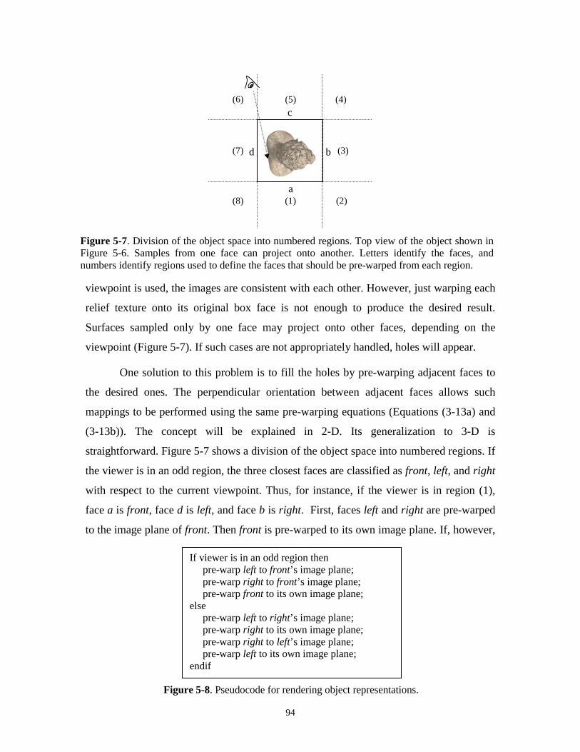
94

viewpoint is used, the images are consistent with each other. However, just warping each

relief texture onto its original box face is not enough to produce the desired result.

Surfaces sampled only by one face may project onto other faces, depending on the

viewpoint (Figure 5-7). If such cases are not appropriately handled, holes will appear.

One solution to this problem is to fill the holes by pre-warping adjacent faces to

the desired ones. The perpendicular orientation between adjacent faces allows such

mappings to be performed using the same pre-warping equations (Equations (3-13a) and

(3-13b)). The concept will be explained in 2-D. Its generalization to 3-D is

straightforward. Figure 5-7 shows a division of the object space into numbered regions. If

the viewer is in an odd region, the three closest faces are classified as front, left, and right

with respect to the current viewpoint. Thus, for instance, if the viewer is in region (1),

face a is front, face d is left, and face b is right. First, faces left and right are pre-warped

to the image plane of front. Then front is pre-warped to its own image plane. If, however,

Figure 5-7. Division of the object space into numbered regions. Top view of the object shown inFigure 5-6. Samples from one face can project onto another. Letters identify the faces, andnumbers identify regions used to define the faces that should be pre-warped from each region.

(1) (2)

(3)

(4)(5)(6)

(7)

(8)a

b

c

d

If viewer is in an odd region then pre-warp left to front’s image plane; pre-warp right to front’s image plane; pre-warp front to its own image plane;else pre-warp left to right’s image plane; pre-warp right to its own image plane; pre-warp right to left’s image plane; pre-warp left to its own image plane;endif

Figure 5-8. Pseudocode for rendering object representations.

95

the viewer is an even region, the two closest faces are classified as left and right. For

instance, if the viewer is in region (8), face d is left and face a is right. First, left is pre-

warped to the image plane of right, then right is pre-warped to its own image plane.

Likewise, right is pre-warped to the image plane of left, and then left is pre-warped to its

own image plane. Figure 5-8 presents the pseudocode for the algorithm. Notice that this

algorithm explicitly defines a set of at most three (in the full 3-D version of the

algorithm) polygons that need to be displayed.

The perpendicular orientation between adjacent faces can be exploited to pre-

warp a face to its adjacent face as if it were the adjacent face itself. When the viewer is in

an odd region, the displacement values associated with left and right are converted to

column indices for front, while their column indices can be used as displacement for front

(Figure 5-9). Thus, left and right can be pre-warped to front as if they were front

Figure 5-9. Displacement values from left and right become column values for front. Columnsfrom left and right become displacement for front.

lefta�

righta�

front

left right

fronta�

viewpoint

Figure 5-10. Images associated with four of the six relief textures used to represent the statue.

96

themselves. The even region is similar.

Figure 5-10 shows the images associated with four relief textures of the statue

shown in Figure 5-6. Despite its complex shape, relief texture mapping produces realistic

renderings of the object at interactive rates. Figure 5-11 shows the statue rendered as two

texture-mapped quadrilaterals (left and right), whose boundaries are shown to the right.

The corresponding pre-warped textures are shown in Figure 5-12 and illustrate the

factorization of the planar perspective component from the pre-warp. Such a distortion is

latter compensated for during the texture mapping stage of the algorithm. A different

view of the statue is shown in Figure 5-13.

Figure 5-11. Reconstructed view of the statue obtained by texture mapping two quads (left).The lines show the boundaries of the polygons (right).

Figure 5-12. Pre-warped textures used to produce the image shown in Figure 5-11.

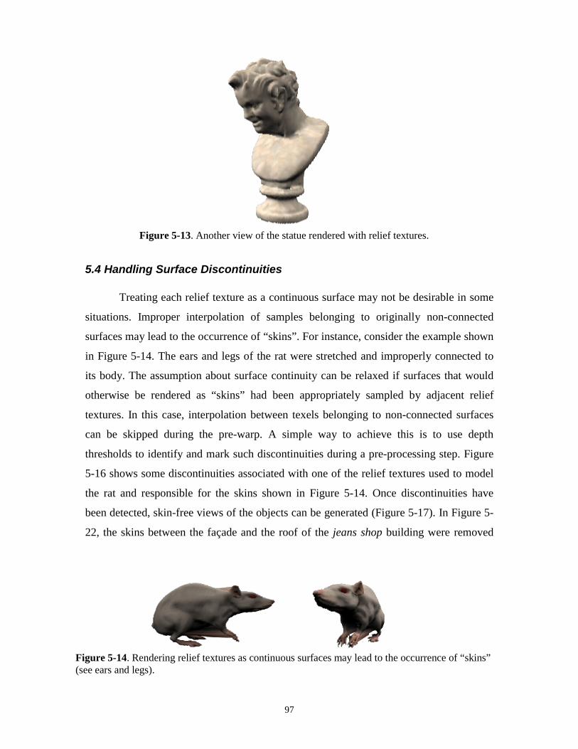
97

5.4 Handling Surface Discontinuities

Treating each relief texture as a continuous surface may not be desirable in some

situations. Improper interpolation of samples belonging to originally non-connected

surfaces may lead to the occurrence of “skins”. For instance, consider the example shown

in Figure 5-14. The ears and legs of the rat were stretched and improperly connected to

its body. The assumption about surface continuity can be relaxed if surfaces that would

otherwise be rendered as “skins” had been appropriately sampled by adjacent relief

textures. In this case, interpolation between texels belonging to non-connected surfaces

can be skipped during the pre-warp. A simple way to achieve this is to use depth

thresholds to identify and mark such discontinuities during a pre-processing step. Figure

5-16 shows some discontinuities associated with one of the relief textures used to model

the rat and responsible for the skins shown in Figure 5-14. Once discontinuities have

been detected, skin-free views of the objects can be generated (Figure 5-17). In Figure 5-

22, the skins between the façade and the roof of the jeans shop building were removed

Figure 5-14. Rendering relief textures as continuous surfaces may lead to the occurrence of “skins”(see ears and legs).

Figure 5-13. Another view of the statue rendered with relief textures.

98

and the use of an extra conventionally texture-mapped polygon seamlessly filled the

resulting hole.

5.5 Correct Occlusions

The relief texture-mapping algorithm, as described so far, does not handle

interpenetrating polygons appropriately. Thus, for example, consider intersecting a planar

polygon with the bounding box used to represent an object. Since the intersection

between two polygons defines a straight line, the resulting occlusion pattern will not

Figure 5-15. Four of the six relief textures used to model the rat of Figure 5-14. Some adjacenttexels in (b) and (d) represent samples from non-connected surfaces.

(a) (b) (c) (d)

Figure 5-17. Same view as in Figure 5-14, rendered after surface discontinuity identification.

Figure 5-16. Skin detection. Surface discontinuities associated with Figure 5-15(b) identifiedafter some user-specified depth thresholds.

99

match the perceived depth of the associated relief textures and will exhibit straight lines

in regions containing nontransparent texels. Figure 5-18 (left) illustrates this situation.

The correct image, rendered using a mesh of micro-polygons, is shown on the right. In

order to avoid this problem, corrected depth values accounting for the perceived off-the-

plane displacements must be computed.

Figure 5-19 shows a 2-D view of a relief texture observed from a center of

projection C� . Let x� be a point in 3-space sampled by texel t, whose coordinates in the

source texture are ),( ss vu . The Z coordinate of x� in camera space when observed from

C� is given by

4321 ),( cvudisplcvcucZ ssssx +++=&

(5-1)

where ncc�� ⋅=1 , nac s

�� ⋅=2 , nbc s

��⋅=3 and nfc s

��⋅=4 are constants for a given viewing

configuration, n�

is the unit vector normal to the image plane of the target camera,

CCc s��� −= , and sC� , sa

�, sb

� and sf

� are the parallel-projection camera parameters

associated with the relief texture. xZ&

can be interpolated along rows and columns in the

same way as described for color in Chapter 4. Also, let ),( jj vu be the coordinates of

texel t ′ obtained after pre-warping t . Notice that the perceived depth at t ′ is xZ&

(Figure

5-19). Alternatively, one can compute and interpolate only the difference z∆ between the

Figure 5-18. Occlusion is checked against the faces of the bounding box, introducing visibilityerrors characterized by straight lines in regions containing nontransparent texels (left). Correctresult obtained by rendering the statue as a mesh of micro-polygons (right). Bounding box shownfor comparison.

100

perceived depth and the actual depth at t ′ , which can be encoded using a smaller number

of bits. Since t ′ is on the source image plane, its Z coordinate in the target camera space

can be expressed as

321 cvcucZ jjt ++=′ .

During the pre-warp, z∆ values can be linearly interpolated along rows and columns.

The interpolated values can be used to compute the amount by which the depth buffer

must be changed to produce correct visibility.

The normalized Z values in device or screen coordinates for point x� is computed

as [Blinn98]:

−

−

=x

nx

nf

fscreenx Z

ZZ

ZZ

ZZ

&

&

&

−=

x

nxscreenx Z

ZZkZ

&

&

&

, (5-2)

where nZ and fZ are the near and far clipping planes, respectively, specified in the target

camera’s coordinate system (Figure 5-19). The amount of z-buffer correction required for

texel t ′ is then given by

screentscreenxscreen ZZz ′−=∆&

C�

image plane

Zn = Znear

Zf = Zfar

t

x.

relief texture

t ′

c�

Figure 5-19. Point x� , originally associated with texel t, projects into texel t ′ after the pre-warping. nZ and fZ are the near and far clipping planes, respectively.

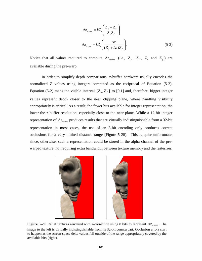
101

−=∆

′

′

tx

txnscreen ZZ

ZZkZz

&

&

∆+∆=∆

′′ tt

nscreen ZzZ

zkZz

)(. (5-3)

Notice that all values required to compute screenz∆ (i.e., xZ&

, tZ ′ , nZ and fZ ) are

available during the pre-warp.

In order to simplify depth comparisons, z-buffer hardware usually encodes the

normalized Z values using integers computed as the reciprocal of Equation (5-2).

Equation (5-2) maps the visible interval ],[ fn ZZ to [0,1] and, therefore, bigger integer

values represent depth closer to the near clipping plane, where handling visibility

appropriately is critical. As a result, the fewer bits available for integer representation, the

lower the z-buffer resolution, especially close to the near plane. While a 12-bit integer

representation of screenz∆ produces results that are virtually indistinguishable from a 32-bit

representation in most cases, the use of an 8-bit encoding only produces correct

occlusions for a very limited distance range (Figure 5-20). This is quite unfortunate,

since, otherwise, such a representation could be stored in the alpha channel of the pre-

warped texture, not requiring extra bandwidth between texture memory and the rasterizer.

Figure 5-20. Relief textures rendered with z-correction using 8 bits to represent screenz∆ . The

image to the left is virtually indistinguishable from its 32-bit counterpart. Occlusion errors startto happen as the screen-space delta values fall outside of the range appropriately covered by theavailable bits (right).

102

An efficient 8-bit encoding solution, whose results are comparable to the

rendering of the actual geometric model, can still be obtained with the quantization of

z∆ . In this approach, one identifies the maximum and minimum z∆ values after

interpolation and uses the same strategy described in Chapter 4. First, a quantization step

is computed as:

−=

254

minmaxqs ,

and the indices for the quantized values are obtained from z∆ using the formula

−∆=qs

zqi

minint .

Notice that, in this case, a single index value has been reserved for transparency, thus

constraining the surface to be either completely transparent or fully opaque. Extra

quantization indices could be traded for extra transparency levels. The computation of the

approximate delta value for a given index qi is given by

qiqsz *min+=′∆ . (5-4)

Figure 5-21 shows the statue rendered with an interpenetrating polygon seen from

different distances. In this example, z∆ was interpolated and the resulting values were

quantized before being used to modulate the depth buffer. The results are virtually

indistinguishable from the rendering of the object as a mesh of micro-polygons.

Figure 5-21. Relief texture rendered with z-correction using 8-bit quantized z∆ values.

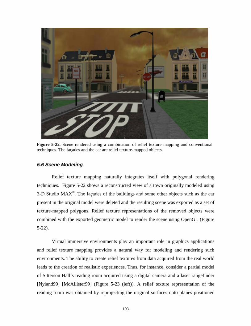
103

5.6 Scene Modeling

Relief texture mapping naturally integrates itself with polygonal rendering

techniques. Figure 5-22 shows a reconstructed view of a town originally modeled using

3-D Studio MAX®. The façades of the buildings and some other objects such as the car

present in the original model were deleted and the resulting scene was exported as a set of

texture-mapped polygons. Relief texture representations of the removed objects were

combined with the exported geometric model to render the scene using OpenGL (Figure

5-22).

Virtual immersive environments play an important role in graphics applications

and relief texture mapping provides a natural way for modeling and rendering such

environments. The ability to create relief textures from data acquired from the real world

leads to the creation of realistic experiences. Thus, for instance, consider a partial model

of Sitterson Hall’s reading room acquired using a digital camera and a laser rangefinder

[Nyland99] [McAllister99] (Figure 5-23 (left)). A relief texture representation of the

reading room was obtained by reprojecting the original surfaces onto planes positioned

Figure 5-22. Scene rendered using a combination of relief texture mapping and conventionaltechniques. The façades and the car are relief texture-mapped objects.

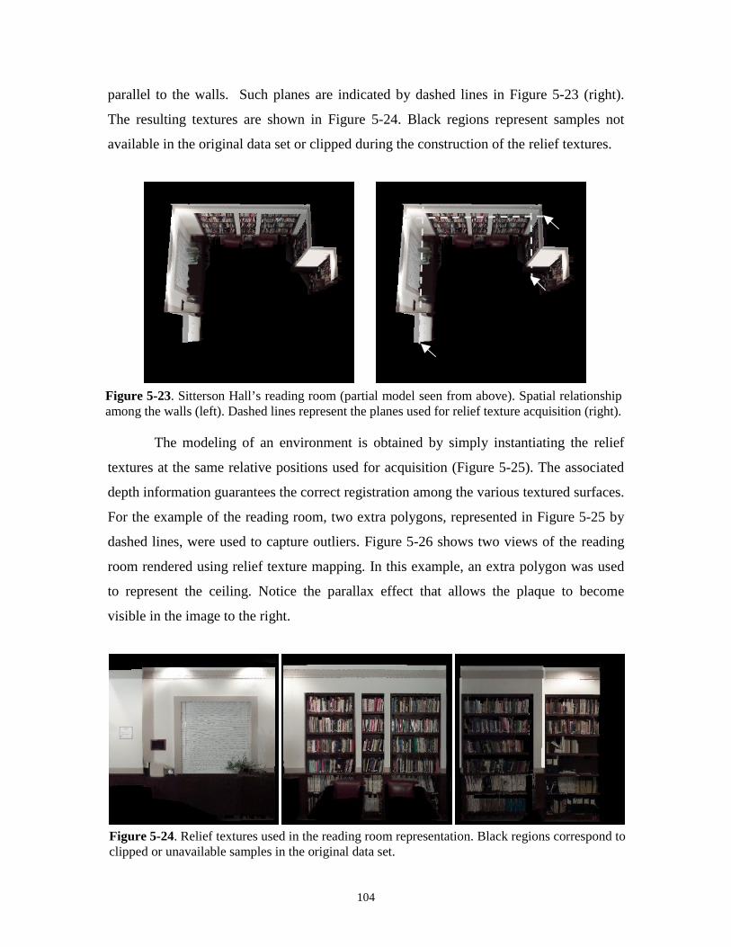
104

parallel to the walls. Such planes are indicated by dashed lines in Figure 5-23 (right).

The resulting textures are shown in Figure 5-24. Black regions represent samples not

available in the original data set or clipped during the construction of the relief textures.

The modeling of an environment is obtained by simply instantiating the relief

textures at the same relative positions used for acquisition (Figure 5-25). The associated

depth information guarantees the correct registration among the various textured surfaces.

For the example of the reading room, two extra polygons, represented in Figure 5-25 by

dashed lines, were used to capture outliers. Figure 5-26 shows two views of the reading

room rendered using relief texture mapping. In this example, an extra polygon was used

to represent the ceiling. Notice the parallax effect that allows the plaque to become

visible in the image to the right.

Figure 5-23. Sitterson Hall’s reading room (partial model seen from above). Spatial relationshipamong the walls (left). Dashed lines represent the planes used for relief texture acquisition (right).

Figure 5-24. Relief textures used in the reading room representation. Black regions correspond toclipped or unavailable samples in the original data set.

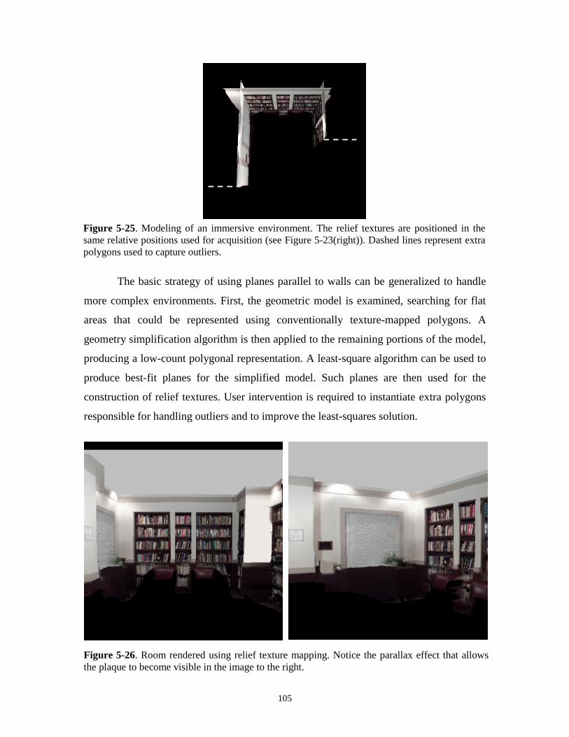
105

The basic strategy of using planes parallel to walls can be generalized to handle

more complex environments. First, the geometric model is examined, searching for flat

areas that could be represented using conventionally texture-mapped polygons. A

geometry simplification algorithm is then applied to the remaining portions of the model,

producing a low-count polygonal representation. A least-square algorithm can be used to

produce best-fit planes for the simplified model. Such planes are then used for the

construction of relief textures. User intervention is required to instantiate extra polygons

responsible for handling outliers and to improve the least-squares solution.

Figure 5-25. Modeling of an immersive environment. The relief textures are positioned in thesame relative positions used for acquisition (see Figure 5-23(right)). Dashed lines represent extrapolygons used to capture outliers.

Figure 5-26. Room rendered using relief texture mapping. Notice the parallax effect that allowsthe plaque to become visible in the image to the right.

106

5.7 Discussion

The mapping of displacement values into column indices for perpendicular faces

introduces a truncation error whose magnitude is bounded by 0.5 texel16. This may,

theoretically, cause minor misregistration problems for isolated pixels along the edge

shared by two perpendicular polygons. The effect of such a truncation is further

minimized by the texture’s spatial coherence, by the existence of other kinds of

discretizations inherent to digital images and by filtering, as discussed in Chapter 4.

Truncation errors seem not to be a concern for the case of relief texture-mapped objects,

since one relief texture containing actual displacement values is always warped to each of

the visible faces of the object’s bounding box. The occurrence of skins may, however,

cause color discontinuities along shared edges in object representations. Although subtle,

such effects can be distracting in animated sequences due to the human’s visual

sensitivity to them. Once skins have been satisfactorily removed, these effects disappear.

Shaded-relief maps have been used in cartography for many years to convey the

illusion of three-dimensionality [Batson75]. More recent, terrain rendering has become an

important component of flight simulators, games and topographic applications, with real-

time visualization of large-scale surfaces attracting the attention of several researchers

[Hoppe98] [Pajarola98]. Although terrain data is usually presented as irregular grids

matching the high-scale details of surfaces, relief texture representation for such data sets

can be easily constructed. Figure 5-27 shows a view of Northern Vancouver, British

Columbia, rendered using relief texture mapping. Such a view corresponds to an area of

approximately 26,000 km2 and was created by patching 25 256x256-texel relief textures

[Hillesland99]. Hillesland used digital orthophotos17 covering Vancouver and the Frasier

Valley in British Columbia [Triathlon95]. Since the elevation data was scattered, a 2-D

Delaunay triangulation was computed and the height associated with each texel was

interpolated [Hillesland99]. Registration between the color images and the elevation data

was performed using Universal Transverse Mercator (UTM) coordinates available for

16 Measured in the texture space associated with the perpendicular face.17 Image maps produced by removing distortions inherent in aerial photography [Triathlon95].

107

both data sets. A close-up of one of the relief textures used to create Figure 5-27,

illustrating the silhouettes of some mountains, is shown in Figure 5-28.

An interesting property of relief texture mapping is its support for dynamic

changes in surface shape. Surface attributes are represented using a linear array and their

values can be easily changed over time. This suggests the use of relief textures to animate

surfaces undergoing changes of both shape and color. The UNC nanoManipulator

[Taylor94] is a virtual-environment interface to a scanned-probe microscope that allows

chemists, biologist and physicists to explore the surface of a material at nanometer scale.

The height values output by the microscope are sent through a network to a 3-D graphics

workstation for visualization. Researchers from the nanoManipulator project have

suggested, and are exploring, visualization strategies based on dynamic relief textures,

which are updated as new data become available from the microscope. Figure 5-29 shows

Figure 5-27. Northern Vancouver rendered using a mosaic of 5 by 5 relief textures created fromaerial photographs and elevation data [Hillesland99].

108

three views of a surface scanned with the probe microscope and rendered using relief

texture mapping.

Yang has explored a combination of post-rendering warp [Mark99] and relief

texture mapping to produce remote rendering of live action [Yang99]. In this approach, a

server acquires and sends color and compressed depth data to remote locations. The scene

is modeled as a set of relief textures whose updates are conditioned to changes in the

original scene. Figure 5-30 illustrates the idea using the DECface model [Waters94]. The

Figure 5-28. Close-up on one of the relief textures used to create Figure 5-27. Notice thesilhouettes of the mountains.

Figure 5-29. Three views of a surface scanned with UNC nanoManipulator scanned-probemicroscope and rendered in gray scale using relief texture mapping.

109

images on the left are views of a deformable polygonal model at the server site while the

images on the right correspond to relief texture-mapping reconstructions from new

viewpoints at the client side. As the facial expression changes (Figure 5-30(a)), updated

data are sent to clients (Figure 5-30(b)).

Figure 5-30. Relief texture created locally (a) and sent to remote sites for visualization fromarbitrary viewpoints (b).

(a) (b)

110

This page left blank intentionally.

111

Chapter 6 – Multiresolution, Inverse Pre-Warping, Clipping and

Shading

Image pyramids have long been used in computer graphics to produce antialiased

texture mapped images at fixed per-pixel cost [Williams83]. This chapter discusses the

construction and use of relief texture pyramids for representing levels of detail and for

antialiasing. Representing each texture using fixed resolution implies a constant amount

of work during the pre-warp, independently of the number of pixels it covers on the

screen. Relief texture pyramids can be used to keep the warping cost proportional to its

contribution to the final image and to reduce the effects of aliasing. The chapter also

describes an inverse pre-warping strategy for relief textures and presents an efficient

incremental algorithm for performing clipping in 1-D. It discusses the use of normal

maps for shading relief textures and the use of the shadow map algorithm [Williams78] to

cast shadows both onto and from relief-texture mapped representations.

Figure 6-1. Relief texture pyramid showing five levels for the front face of the statue. From leftto right the dimensions of the textures are respectively 256x256, 128x128, 64x64, 32x32 and16x16 texels.

112

6.1 Relief Texture Pyramids

A relief texture pyramid is a set { }+∈≤= − ZmlmlTP lm ,;:2

, where lmT −2 is a relief

texture with dimensions lmlm x −− 22 associated with level l of the pyramid and m is its

maximum level (Figure 6-1). lmT −2 is obtained by averaging color and depth data of

groups of ll x22 adjacent texels in the highest resolution relief texture (level zero). Only

texels representing actual surface samples18 are considered during the averaging process.

The lengths of vectors a�

and b�

(camera parameters representing the horizontal and

vertical sample spacing, respectively) are doubled from level l to level 1+l of the

pyramid, i.e., 02 aa ll

�� = , 02 bb ll

��= , where subscripts identify the levels. This

compensates for the halving of the number of texels in each dimension between levels l

and 1+l , thus keeping the spatial coverage of the relief texture unchanged.

Relief texture pyramids provide a unified representation for implementing both levels

of detail and antialiasing. Levels of detail (LODs) are pre-computed simplified object

representations used to reduce the number of rendered primitives at a given time. During

the rendering, a representation is selected based on the object’s estimated contribution to

the final image. Relief texture pyramids can be regarded as realizations of image-based

LODs19 and can also be used for antialiasing, exploiting the filtering capabilities

available in texture mapping hardware.

A multiresolution object representation consists of six relief-texture pyramids, one for

each face of the object’s bounding box. Figures 6-2 shows the first four levels of such an

object representation rendered using the same algorithms described in previous chapters.

Examples of image-based LODs mapped onto two quadrilaterals are shown in Figures 6-

3 and 6-4. 128x128-texel relief textures (level 1) were used to create Figure 6-3. Figure

6-4 was produced using 64x64-texel relief textures (level 2) and shows the same object at

three different distances. A level 0 rendering of the same view is shown in Figure 5-11.

18 Transparent samples are ignored.19 Mip-map pyramids [Williams83] are the simplest example of (static) image-based LODs.

113

Selection of geometric LODs is usually based on a user specified pixel error

requirement [Erikson99]. By estimating the maximum error (in object space) introduced

by the simplification algorithm and projecting such an error onto the view plane, a screen

space error is obtained [Erikson99]. Although automatic level selection for textured

LODs has not been implemented, it can be based on the projected areas of the associated

quadrilaterals. Figure 6-5 shows a distant object rendered using texture LODs produced

at different levels of a relief texture pyramid. From left to right, the source textures used

for warping consist of 256x256, 128x128, 64x64, 32x32 and 16x16 texels, respectively.

Figure 6-3. Textured LOD produced with 128x128-texel relief textures. The corresponding pre-warped textures are shown on the right.

Figure 6-2. Image-based LODs rendered using the first four levels of an object’s multiresolutionrepresentation, whose front images are shown in Figure 6-1.

114

For this example, the renderings produced with levels 0 and 1 (first and second images

from left to right) are unnecessarily expensive and more prone to aliasing. Levels 2 and 3

produce acceptable results with significantly less work.

6.1.1 Bilinear versus trilinear filtering

Higher-order filters are usually regarded as producing better results than lower-

order filters when used for image reconstruction and resampling. In texture mapping

applications, trilinear interpolation is often preferred to bilinear interpolation for image

resampling despite being computationally more expensive and usually introducing

excessive blurring (Figure 6-6). For relief texture mapping, however, bilinear

interpolation is the preferred resampling method.

Although mip maps [Williams83] are very effective for reducing aliasing artifacts

due to texture minification, such an issue is not crucial in the texture map stage of the

relief texture mapping algorithm. Also, the distinction between the apparent distance of a

Figure 6-6. Checkerboard texture mapped using bilinear (left) and trilinear (mip mapped)resampling (right).

Figure 6-5. A distant object rendered using textured LODs. From left to right: 256x256,128x128, 64x64, 32x32 and 16x16-texel relief textures were used for the warping. Imageresampling was performed using bilinear interpolation.

Figure 6-4. Views of a textured LOD rendered from different distances using 64x64-texel relieftextures.

115

rendered surface and the actual distance of the texture-mapped polygon is an important

aspect to be considered. Both topics are discussed next.

Consider the situation depicted in Figure 6-7, where a building façade is observed

at a grazing angle through a viewing plane. The pre-warp causes samples whose

projections are adjacent on the viewing plane to also be adjacent in the pre-warped

texture. Thus, samples that need to be averaged together for antialiasing purposes are

always close to each other and bilinear interpolation suffices to produce satisfactory

resampling. Figure 6-8 shows the renderings of the view represented in Figure 6-7 using

both bilinear (left) and trilinear filtering (right). The results are very similar except that

the image resampled using bilinear interpolation is sharper. Trilinear filtering, on the

other hand, produced better antialiased contours (Figure 6-8).

The second argument against the use of trilinear interpolation for relief texture

mapping has to do with the difference between the apparent distance of a surface and the

actual distance of the associated texture-mapped polygon(s). While an observer perceives

the apparent distance of the surface, conventional mip map level estimation algorithms

try to keep the ratio between pixel and texel sizes equal to one. For this reason, they are

not suitable for projective-based representations such as the perpendicular plane

representation used for objects. For example, consider the rendering shown in Figure 6-9.

The difference between the projected areas of the two quadrilaterals leads to the selection

of different mip map levels for rendering each polygon. This causes regions perceived as

Figure 6-7. Façade observed from a grazing angle. The perspective effect causes the tip of theroof ornament to project closer to the viewer onto the source image plane (dot).

source image plane

116

spatially close to each other to exhibit different amounts of blurring. In the case of Figure

6-9, the forehead and nose are blurrier than other parts of the statue.

An approximation to trilinear filtering capable of reducing both rendering costs

and aliasing artifacts can be achieved by combining LOD selection with bilinear

resampling. Such a strategy was used to render the views of the statue in Figure 6-5.

6.1.2 Cost considerations

The use of bilinear interpolation for texture resampling also has some

computational advantages over the use of mip map filtering. Thus, let T be a nxn relief

texture whose projection, from a viewpoint V , covers p pixels on the screen. Assuming

that the texture mapping resampling is performed using bilinear interpolation, the worst–

Figure 6-8. Building façade pre-warped and then texture mapped using bilinear (left) andtrilinear (mip mapping) resampling (right).

Figure 6-9. Conventional mip map level estimation algorithms are not suited for projection-based representations. The image containing the forehead and nose is blurrier than the other one.

117

case rendering cost for T adds up to 2n warps and p bilinear filtering operations. If,

however, trilinear resampling is used, the worst-case rendering cost amounts to 2n warps,

31..

44

2

2

22 nnnf ≅+++= averaging operations applied to groups of four adjacent texels

(for the construction of the mip map) and p trilinear filtering operations. Trilinear

interpolation also requires twice as much bandwidth between the texture memory and the

rasterizer as bilinear interpolation. Moreover, the pre-warp needs to be performed every

time the viewer moves and, in this case, a new mip map needs to be created.

6.2 Inverse Pre-Warping

Ideally, only texels effectively contributing to some screen fragment should be

pre-warped. Unfortunately, such an optimal strategy is not practical for interactive

applications. In the case of the pre-warp, Equations (3-13a) and (3-13b) define many-to-

one mappings and, therefore, are not invertible (Figure 6-10). Inverting them would be

equivalent to solving the following indeterminate system

),()),(1( 13 ssssis vudisplkvudisplkuu −+=

),()),(1( 23 ssssis vudisplkvudisplkvv −+= .

Without knowing (or introducing additional restrictions to) the value of ),( ss vudispl , the

system accepts multiple solutions. Thus, any inverse approach has to search for the

Figure 6-10. Two source texels are mapped to the same location in the pre-warped image. Thepre-warping equations define many-to-one mappings and cannot be directly inverted.

118

closest sample from the viewpoint along each target ray 20.

6.2.1 Searching along epipolar lines

Although inverse mapping solutions ultimately require a search to be performed,

this search can be performed along segments of epipolar lines. The approach described

here is similar to the inverse warping methods of McMillan and Bishop [McMillan97]. In

this case, however, only the pre-warping is being inverted, allowing the algorithm to be

efficiently implemented using simple incremental computations. Nevertheless, it has no

significant advantages over the forward approach described in the previous chapters and

is presented here for completeness.

Consider the situation illustrated in Figure 6-11, where fcd�� ⋅= is the distance

between the viewer to the source image plane, ev is the row coordinate of the epipole and

c�

is the vector from the target COP to the origin of the source image plane. f�

is the unit

vector normal to the source image plane (Figure 3-17). Let iv be the row coordinate of

the intersection of the source image plane with the viewing ray through p� (Figure 6-11).

From similar triangles,

20 This assertion also applies to the “inverse” rendering of all kinds of range images.

Figure 6-11. Two-dimensional representation of the search strategy used for an inverse pre-warper.

c�

iv1−pv

pv

d

ev

p.

source image plane

119

)()( ip

p

ei vv

displ

vv

d

−=

−, (6-1)

where pdispl is the displacement value associated with p� . Equation (6-1) can be

rewritten as

pvip vcdispl ∆= ,

where ipp vvv −=∆ .

The search for the visible sample through iv should then start at iv and proceed in

the opposite direction to the epipole21, ending when Inequality (6-2) is satisfied for a

given source texel with row coordinate sv , displacement sdispl and iss vvv −=∆ .

svis vcdispl ∆≤ (6-2)

In 3-D, the search should stop when the condition

suis ucdispl ∆≤ and svis vcdispl ∆≤

is satisfied. In this case, uic and su∆ are the column analogs of vic and sv∆ ,

respectively. For each pre-warped texel ),( ii vu , this search proceeds along the epipolar

line corresponding to the parallel projection of the ray passing through the target COP

and ),( ii vu onto the source image plane. Since the source and target image planes do not

coincide in general, the resulting image still needs to be texture mapped onto the source

image plane.

6.3 One-dimensional Clipping

Skipping the pre-warp for samples having zero displacement speeds up the

rendering of relief textures, as discussed in Chapter 3. Another way to accelerate the

rendering is to avoid transforming samples whose projections fall outside of the limits of

the source image plane. This section presents a 1-D clipping algorithm for use during the

pre-warp. It will be described in the context of relief textures, but the same ideas also

apply to perspective projection images with depth.

21 Assuming that all samples are behind the source image plane, such as the case shown in Figure6-11, no texels closer to the epipole than iv can possibly map to iv .

120

Consider the two-dimensional representation depicted in Figure 6-12, where P is

the plane defined by the target COP and by the two vertices of the source image plane

associated with mu , the extremum column closest to the COP. According to Figure 6-12,

all samples outside of the shaded region project beyond the limits of the source image

plane. Thus, let st be a source texel at column su whose corresponding sample ss lies on

P (Figure 6-12). Also, let ur be the ratio

s

su u

displr

∆= ,

where sms uuu −=∆ , sdispl is the displacement value associated with st and ur is the

tangent of the angle between P and the source image plane. Thus, for any given source

texel jt , jt projects onto the source image plane if and only if

juj urdispl ∆≤ . (6-3)

Notice that if splatting is used for reconstruction, all samples not satisfying

Inequality (6-3) can be automatically clipped. Extra care must be taken if linear

interpolation is used for reconstruction, such as the case of the two-pass 1-D approach.

For instance, consider the situation of sample 1+ks shown in Figure 6-12. Although its

projection falls outside the limits of the source image plane, the column coordinate of its

projection is still required to appropriately interpolate colors between 1+ks and its visible

Figure 6-12. Clipping (top view). All samples whose outside the shaded triangle project beyondthe limits of the source image plane.

ks

ss

1+ks

mususource image plane

P

121

neighbor ks . The necessary condition for performing clipping in 1-D follows: given three

consecutive texels 1−kt , kt and 1+kt on the same row, such that none of them satisfies

Inequality (6-3), the warp of kt can be safely skipped. A similar property applies to

columns. In this case, Inequality (6-3) becomes

jvj vrdispl ∆≤ , (6-4)

where βtan=vr and jms vvv −=∆ have analogous definitions to ur and su∆ ,

respectively. Thus, clipping can be efficiently implemented during both the horizontal

and the vertical passes of the pre-warp by checking the conditions defined by Inequalities

(6-3) and (6-4), respectively, for groups of three consecutive texels.

6.4 Shading

Image-based rendering techniques can create photo-realistic pictures from images,

thus avoiding expensive simulations of surface-light interactions. Such a property not

only leads to considerable computational savings but also provides a simple way to

represent and render complex physical processes. Unfortunately, the photometric

properties of many materials cannot be represented using just a few pictures. For

instance, the appearance of non-diffuse surfaces changes with viewpoint and illumination

direction. For these surfaces, correct rendering would require the use of huge image

databases to store their appearance from arbitrary viewpoints. The Light Field [Levoy96]

and Lumigraph [Gortler96] approaches approximate such a solution. If the scene

illumination is allowed to vary, storage requirements become even bigger [Wong97].

A simple approach capable of producing local illumination solutions22 consists of

extending image-based representations with surface normals. Normals are geometric

properties of surfaces and therefore do not change with viewpoint. They can be

interpolated during the pre-warp and used by a deferred shading strategy to compute

view-dependent effects. Normal maps are special kinds of texture maps that store normal

vector components instead of color data [Fournier92]. Multiresolution representations for

22 Local illumination solutions only account for direct illumination, not considering lightcontributions resulting from multiple inter-reflections.

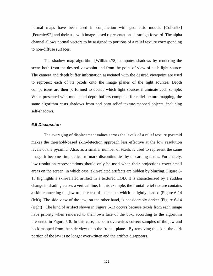
122

normal maps have been used in conjunction with geometric models [Cohen98]

[Fournier92] and their use with image-based representations is straightforward. The alpha

channel allows normal vectors to be assigned to portions of a relief texture corresponding

to non-diffuse surfaces.

The shadow map algorithm [Williams78] computes shadows by rendering the

scene both from the desired viewpoint and from the point of view of each light source.

The camera and depth buffer information associated with the desired viewpoint are used

to reproject each of its pixels onto the image planes of the light sources. Depth

comparisons are then performed to decide which light sources illuminate each sample.

When presented with modulated depth buffers computed for relief texture mapping, the

same algorithm casts shadows from and onto relief texture-mapped objects, including

self-shadows.

6.5 Discussion

The averaging of displacement values across the levels of a relief texture pyramid

makes the threshold-based skin-detection approach less effective at the low resolution

levels of the pyramid. Also, as a smaller number of texels is used to represent the same

image, it becomes impractical to mark discontinuities by discarding texels. Fortunately,

low-resolution representations should only be used when their projections cover small

areas on the screen, in which case, skin-related artifacts are hidden by blurring. Figure 6-

13 highlights a skin-related artifact in a textured LOD. It is characterized by a sudden

change in shading across a vertical line. In this example, the frontal relief texture contains

a skin connecting the jaw to the chest of the statue, which is lightly shaded (Figure 6-14

(left)). The side view of the jaw, on the other hand, is considerably darker (Figure 6-14

(right)). The kind of artifact shown in Figure 6-13 occurs because texels from each image

have priority when rendered to their own face of the box, according to the algorithm

presented in Figure 5-8. In this case, the skin overwrites correct samples of the jaw and

neck mapped from the side view onto the frontal plane. By removing the skin, the dark

portion of the jaw is no longer overwritten and the artifact disappears.

123

Image re-shading is a difficult problem. Whereas evaluating shading expressions

for each sample of a range image is straightforward, removing light, deleting shadows,

and maintaining consistent illumination among several image-based representations in a

scene are not trivial tasks [Fournier93] [Oliveira98]. All these operations require

knowledge about the properties of the light sources involved. Reference images may also

record the result of light interaction with objects not represented in the pictures, such as

Figure 6-14. Front and right relief textures of the statue representation (level 0). The regionresponsible for the skin-related artifact is highlighted.

Figure 6-13. Skin-related artifact caused by large difference in the shading of a region aroundthe chin as viewed by two adjacent relief textures (Figure 6-14).

124

the case of caustics and shadows cast by objects clipped from the image’s field of view.

In general, a substantial amount of information is needed to change the illumination in a

picture consistently.

6.6 Summary

This chapter has covered a variety of topics including multiresolution

representations for relief textures, inverse pre-warping, clipping and shading.

Multiresolution representations are constructed by averaging color and displacement

values of groups of adjacent texels and are similar to mip map pyramids. The resulting

LOD representations are rendered using the same algorithms described in previous

chapters.

The use of bilinear interpolation for the texture resampling presents some

advantages over trilinear filtering when used for relief texture mapping. While mip

mapping is very effective for reducing aliasing artifacts caused by texture minification,

pre-warp images tend to require little amounts of minification. Thus, bilinear

interpolation produces sharper images, is less prone to undesirable blurring due to

polygonal orientation with respect to the screen, and is computationally less expensive

than trilinear interpolation. Combining LOD selection and bilinear resampling can

approximate trilinear filtering.

The discussion about scene rendering was extended to include shadows. Once the

depth buffer has been modulated to account for relief occlusions, the shadow map

algorithm [Williams78] can be used to cast shadows both onto and from relief texture-

mapped representations. This chapter has also discussed an inverse pre-warping strategy

and presented an efficient incremental algorithm for performing 1-D clipping on the fly.

125

Chapter 7 – Conclusions and Future Work

The idea of texture mapping, i.e., the ability to assign properties to surfaces, is

one of the most powerful concepts in computer graphics. It has been explored and

extended in many ways to produce realistic images, create impressive effects and

accelerate rendering. This research has presented one more extension: the ability to

represent three-dimensional surface details and view-motion parallax. This closing

chapter returns to the issue of one-dimensional warp and reconstruction and explains why

it works. It also provides additional discussions on view-dependent texture mapping and

image-based representations for dynamic environments. The chapter ends with a

summary of the major points presented in this dissertation and with a list of suggested

areas for future exploration.

7.1 Why One-Dimensional Warp and Reconstruction Works

The surprisingly good results produced by 1-D warp and reconstruction strategies

follow from spatial-coherence preservation under projective mappings: groups of

spatially adjacent samples in 3-D are projected onto nearby pixels of an image plane23.

Remember that the pre-warp is just a reprojection of a range image from a new COP.

Together with the separability of perspective projection into orthogonal components,

spatial-coherence preservation guarantees that although samples are shifted along

independent rows (columns), their movements are consistent with the movements of their

original neighbors. Thus, linear interpolation produces good reconstruction for

continuous surfaces in both passes of the pre-warp. This argument supports the use of

two-pass 1-D interpolation for all view-independent surface attributes, such as normal

fields, and for camera-space Z values as discussed in Section 5.5. The resulting normal

23 The converse, though, is not true, mainly because of view-motion parallax, i.e., adjacent pixelsin one image may come from distant samples in 3-D.

126

and depth maps are likely to be as good as the reconstructed intensity image for diffuse

surfaces.

The occurrence of depth discontinuities causes regions of a source image to be

expanded as a result of a parallax effect and are the major cause of source image topology

disruption. Such expansions correspond to the exposure of surfaces not represented in the

original image (skins). Even in the presence of depth discontinuities, the results produced

by one-dimensional resampling are satisfactory for most practical situations, as discussed

in Section 4.7.

7.2 Discussion

7.2.1 View-Dependent Texture Mapping

View-dependent texture mapping [Debevec98] consists of selecting and blending

textures pre-acquired from directions that approximate the desired view. In this case, an

underlying geometric model determines the shape of the surfaces. Relief texture

mapping, on the other hand, creates an illusion of three-dimensionality by projecting

textures, specifically warped for the desired view, onto planar or box-shaped models. It

is, therefore, a projective view-dependent texture-mapping algorithm. Unlike the

blending strategies used in conventional approaches, relief texture mapping is based on a

texture reconstruction strategy that uses a small set of source images.

7.2.2 Dynamic Environments

Virtual reality applications, games and animations often need to continuously

update position, orientation and shape of objects in a scene. By treating each object as a

separate entity, geometry-based approaches naturally support such changes. Relief

textures are hybrid representations and can be used to construct dynamic environments.

Moreover, data associated with relief textures can be changed incrementally over time to

produce morphing effects, such as the case of the face shown in Figure 5-30.

127

7.2.3. Depth Complexity Considerations

A relief texture is a single-layer image representation. Under the surface

continuity assumption, the entire scene has a depth complexity of one and there is no

need for multiple samples along each ray. Objects, on the other hand, are represented

with six perpendicular relief textures, which is equivalent to a multi-layer representation.

Thus, for instance, in Figure 6-14, the combined samples from the left and right images

contain information about the front part of the jaw and from the neck, which are not

visible in any of the individual images simultaneously.

If one wants to remove skins from individual relief textures, such as the walls of

the reading room shown in Figure 5-24, holes may appear. In this case, alternative

representations such as layered-depth images (LDIs) [Shade98] could be used. However,

reconstruction of LDIs is limited to splatting. The existence of multiple samples along

each ray introduces ambiguity about which samples should be connected, making 1-D

interpolation and mesh-based reconstruction impractical. Alternatively, creating and

rendering several layers, each consisting of individual relief textures can be used to

produce similar results. In the supporting animation entitled “Town Exploration Using

Relief Texture Mapping”, the skin between the façade ornament and the roof of one of

the buildings (Jeans Store) was removed and the resulting hole was seamlessly filled by

adding an extra conventionally texture-mapped polygon.

7.2.4. 3-D Photography

In the near future, one can expect the development and popularization of new

devices for simultaneous acquisition of color and depth data. 3-D photography should

then become a standard part of the computer graphics modeling repertoire, and relief

texture mapping offers a suitable strategy for rendering such primitives.

7.3 Synopsis

This dissertation has presented an extension to texture mapping that supports the

representation of three-dimensional surface details and view-motion parallax. This

approach results from the factorization of the 3-D image warping equation of McMillan

128

and Bishop [McMillan97] into a pre-warp followed by standard texture mapping. The

pre-warp is applied to images with per-texel displacements and handles only the parallax

effects resulting from the direction of view and the displacements of texture elements.

The subsequent texture-mapping operation handles the transformation from texture to

screen coordinates. By doing so, relief texture mapping takes advantage of the efficiency

of forward transforms to solve visibility issues, while exploring the superior filtering

capabilities of inverse mappings.

Pre-warping equations for both parallel and perspective-projection images with

depth have been derived and 1-D algorithms for performing clipping, hidden surface

removal, image reconstruction and anti-aliasing have been presented. The use of a depth

buffer modulation strategy for achieving correct occlusions and allowing shadow

computation was described.

The one-dimensional nature of the pre-warping equations follows from the

separability of the perspective projection into orthogonal components. The effectiveness

of 1-D warp and reconstruction strategies results from the spatial coherence preservation

under projective mappings and from the separability of perspective projection.

I have presented algorithms for modeling and rendering three-dimensional objects

and immersive environments using relief textures. The use of quantized displacement

values makes the storage requirements of relief textures equivalent to the requirements of

regular textures, without apparent image degradation. Quantized displacement values can

be used in combination with lookup tables to reduce the computational cost associated

with the pre-warping of one texel to essentially two additions and two multiplications.

I have shown how to construct and render multiresolution representations for

range images. These can be used to reduce aliasing artifacts and to keep the rendering

cost of relief textures proportional to their contribution to the final image. Bilinear

interpolation is the preferred image resampling strategy during the texture mapping stage

of the relief texture-mapping algorithm. It produces sharper images, is less prone to

undesirable blurring due to polygon orientation and is computationally less expensive

than trilinear interpolation.

129

Relief texture mapping naturally integrates itself with current graphics APIs and

provides a framework for combining the photo-realistic promise of image-based

modeling and rendering techniques with the advantages of polygonal rendering.

7.4 Future Work

Some possible areas for further exploration include hardware design for relief

texture mapping, automatic or semi-automatic extraction of relief textures from scenes,

use of relief textures for geometry simplification, and representation of non-diffuse

surfaces.

7.4.1 Hardware implementation

One important area for future investigation is the design of efficient hardware

implementations for relief texture mapping using the derived pre-warping equations.

Adding this pre-warping capability to the texture memory of a graphics accelerator may

allow relief texture mapping to become as commonly used as conventional texture

mapping.

7.4.2 Extraction of relief textures and geometric simplification

Automatic or semi-automatic extraction of relief textures from 3-D environments

and geometry simplification are two important related areas for exploration. A semi-

automatic procedure that combines geometry simplification and least-squares solutions

has been outlined in Section 5-6. Such a strategy serves both purposes at once, as it helps

to identify areas that could benefit most from relief representations, while replacing flat

regions with conventionally texture-mapped polygons.

7.4.3 Representations for non-diffuse surfaces

The striking realism obtained with the use of image-based rendering techniques is

attenuated as the viewer perceives incorrect shading clues, such as fixed highlights, on

non-diffuse surfaces. Highlights produced with Phong shading are unconvincing for most

130

materials, and new algorithms for reshading photographs, accounting for more believable

view-dependent effects, are required.

131

Bibliography

[Aliaga99] Aliaga, D. et al. “MMR: An Integrated Massive Model Rendering SystemUsing Geometric and Image-Based Acceleration”. Proceedings of 1999ACM Symposium on Interactive 3D Graphics. Atlanta, Ga, April 26-28,1999, pp. 199-206.

[Batson75] Batson, R., Edwards, K., Eliason, E. “Computer-Generated Shaded-ReliefImages”. Journal of Research U.S. Geol. Survey, Vol. 3, No. 4, July-Aug.1975, pp. 401-408.

[Blinn76] Blinn, J., Newell, M. “Texture and Reflection in Computer GeneratedImages”. Communications of ACM, Vol. 19, No. 10, October 1976, pp.542-547.

[Blinn78] Blinn, J. “Simulation of Wrinkled Surfaces”. Proc. SIGGRAPH 78 (July1978). In Computer Graphics Proceedings. Annual Conference Series,1978, ACM SIGGRAPH, pp. 286-292.

[Blinn90] Blinn, J. “The Truth About Texture Mapping”. IEEE Computer Graphicsand Applications. March, 1990, pp. 78-83.

[Blinn98] Blinn, J. “W Pleasure, W Fun”. IEEE Computer Graphics andApplications. May, 1998, pp. 78-82.

[Catmull74] Catmull, E. “A Subdivision Algorithm for Computer Display of CurvedSurfaces”. Ph.D. Dissertation, Department of Computer Science,University of Utah, December 1974.

[Catmull80] Catmull, E., Smith, A. “3D Transformations of Images in Scanline Order”.Proc. SIGGRAPH 80 (Seattle, Washington, July 14-18, 1980). InComputer Graphics Proceedings. Annual Conference Series, 1980, ACMSIGGRAPH, pp. 279-285.

[Cohen98] Cohen, J., Olano, M., Manocha, D. “Appearance-PreservingSimplification”. Proc. SIGGRAPH 98 (Orlando, FL, July 19-24, 1998). InComputer Graphics Proceedings. Annual Conference Series, 1998, ACMSIGGRAPH, pp. 115-122.

[Cook84] Cook, R. “Shade Trees”. Proc. SIGGRAPH 84 (July 1984). In ComputerGraphics Proceedings. Annual Conference Series, 1984, ACMSIGGRAPH, pp. 223-231.

[Cox98] Cox, M., Bhandari, N., Shantz, M. “Multi-Level Caching for 3D GraphicsHardware”. Proceedings of the International Symposium on ComputerArchitecture. Barcelona, Spain, June 27 to July 1st, 1998.

[Debevec96] Debevec, P., Taylor, C., Malik, J. “Modeling and Rendering Architecturefrom Photographs: A hybrid geometry- and image-based approach”. Proc.SIGGRAPH 96 (New Orleans, LA, August 4-9, 1996). In ComputerGraphics Proceedings. Annual Conference Series, 1996, ACMSIGGRAPH, pp. 11-20.

132

[Debevec98] Debevec, P., Yu, Y., Borshukov, G. “Efficient View-Dependent Image-Based Rendering with Projective Texture-Mapping”. Proceedings of the9th Eurographics Workshop on Rendering. Vienna, Austria, June 1998.Rendering Techniques ’98, Springer-Verlag, pp. 105-116.

[Erikson99] Erikson, K., Manocha, D. “GAPS: General and Automatic PolygonalSimplification”. Proceedings of 1999 ACM Symposium on Interactive 3DGraphics. Atlanta, Ga, April 26-28, 1999, pp. 79-88.

[Euclid] Euclid. The Thirteen Books of THE ELEMENTS. Vol.3, Book XI, page298. Second Edition Unabridged. Translated by Sir Thomas Heath. DoverPublications, Inc.

[Fant86] Fant, Karl. “A Nonaliasing, Real-Time Spatial Transform Technique”.IEEE Computer Graphics and Application, Vol. 6, No 1, January 1986,pp. 71-80.

[Foley90] Foley, J. et al. Computer Graphics: Principles and Practice. 2nd Edition.Addison-Wesley, 1990.

[Foley00] Foley, J. et al. “Getting There: The Ten Top Problems Left”. IEEEComputer Graphics and Application, Vol. 20, No 1, January 2000, pp. 66-68.

[Fournier92] Fournier, A. “Normal Distribution Functions and Multiple Surfaces”.Graphics Interface ‘92 Workshop on Local Illumination. pp. 45-52.

[Fournier93] Fournier, A., Gunawan, A., Romanzin, “Common Illumination betweenReal and Computer Generated Scenes”. Graphics Interface ‘93, Toronto,Canada. pp. 254-262.

[Gomes97] Gomes, J., Velho, L. Image Processing for Computer Graphics. Springer-Verlag, 1997.

[Gortler96] Gortler, S., et al.. “The Lumigraph”. Proc. SIGGRAPH 96 (New Orleans,LA, August 4-9, 1996). In Computer Graphics Proceedings. AnnualConference Series, 1996, ACM SIGGRAPH, pp. 43-54.

[Grossman98] Grossman, J., Dally, W. “Point Sample Rendering”. Proceedings of the 9th

Eurographics Workshop on Rendering. Vienna, Austria, June 1998.Rendering Techniques ’98, Springer-Verlag, pp. 181-192.

[Hakura97] Hakura, Z., Gupta, A. “The Design and Analysis of a Cache Architecturefor Texture Mapping”. Proceedings of the 24th International Symposiumon Computer Architecture, pp. 108-120.

[Heckbert82] Heckbert, P. “Color Quantization for Frame Buffer Display”. SIGGRAPH82. In Computer Graphics Proceedings. Annual Conference Series, 1982,ACM SIGGRAPH, pp. 297-307.

[Heckbert89] Heckbert, P. Fundamentals of Texture Mapping. Master’s thesis. TechnicalReport No. UCB/CSD 89/516. Computer Science Division, University ofCalifornia, Berkeley.

133

[Heckbert97] Heckbert, P., Garland, M. “Survey of Polygonal Survey SimplificationAlgorithms”. Draft of Carnigie Mellon University Computer ScienceTechnical Report, 1997.

[Hillesland99] Hillesland, K. Interactive, 3D Visualization of Terrain Data Overlaid withAerial Photographs. http://www.cs.unc.edu/~khillesl/comp258/project.html, 1999.

[Hoppe98] Hoppe, H. “Smooth View-Dependent Level-of-Detail Control and itsApplication to Terrain Rendering”. IEEE Visualization’98, ResearchTriangle Park, NC. October 18-23, 1998. pp. 35-42.

[Irani96] Irani, M., Anandan, P. “Parallax Geometry of Pairs of Points for 3D SceneAnalysis”. European Conference on Computer Vision, pp. I:17-30,Cambridge, England, April 1996.

[Irani97] Irani, M., Rousso, B., Peleg, S. “Recovery of Ego-Motion Using RegionAlignment”. IEEE Transactions on Pattern Analysis and MachineIntelligence, Volume 19, No. 3, pp. 268-272, March 1997.

[Kumar94] Kumar, R., Anandan, P., Hanna, K. “Direct Recovery of Shape fromMultiple Views: A Parallax Based Approach”. In Twelfth InternationalConference on Pattern Recognition (ICPR’94), Volume A, pp. 685-688.IEEE Computer Society Press, Jerusalem, Israel, October 1994.

[Levoy96] Levoy, M., Hanrahan, P. “Light Field Rendering”. Proc. SIGGRAPH 96(New Orleans, LA, August 4-9, 1996). In Computer GraphicsProceedings. Annual Conference Series, 1996, ACM SIGGRAPH, pp. 31-42.

[LightPack] LightPack: Light Field Authoring and Rendering Package. StanfordComputer Graphics Laboratory. http://www-graphics.stanford.edu/software/lightpack/.

[Maciel95] Maciel, P., Shirley, P. “Visual Navigation of Large Environments UsingTexture Clusters”. Proceedings of 1995 ACM Symposium on Interactive3D Graphics. Monterey, CA, April 9-12, 1995, pp.95-102.

[Mark99] Mark, W. Post-Rendering 3D Image Warping: Visibility, Reconstruction,and Performance for Depth-Image Warping. Ph.D. Dissertation. UNCComputer Science Technical Report TR99-022, University of NorthCarolina, April 21, 1999.

[McAllister99]McAllister, D. et al. “Real-Time Rendering of Real-World Environments”.Proceedings of the 10th Eurographics Workshop on Rendering. Granada,Spain, June 1999. Rendering Techniques ’99, Springer-Verlag, pp. 145-160.

[McMillan97] McMillan, L. An Image-Based Approach to Three-Dimensional ComputerGraphics. Ph.D. Dissertation. UNC Computer Science Technical ReportTR97-013, University of North Carolina, April 1997.

134

[Nyland99] Nyland, L. et al. “The Impact of Dense Range Data on ComputerGraphics”. Proceedings of Multi-View Modeling and Analysis Workshop(MVIEW99), (Part of CVPR99), Fort Collins, CO, June 1999. pp. 3-10.

[Oliveira98] Oliveira, M., Bishop, G. “Dynamic Shading in Image-Based Rendering”.UNC Computer Science Technical Report TR98-023, University of NorthCarolina, May 31, 1998.

[Oliveira99] Oliveira, M., Bishop, G. “Image-Based Objects”. Proceedings of 1999ACM Symposium on Interactive 3D Graphics. Atlanta, Ga, April 26-28,1999, pp. 191-198.

[Paeth90] Paeth, A. “A Fast Algorithm for General Raster Rotations”. GraphicsGems, Andrew Glassner, Editor. Academic Press, 1990, pp. 179-195.

[Pajarola98] Pajarola, R. “Large Scale Terrain Visualization Using The RestrictedQuadtree Triangulation”. IEEE Visualization ’98, Research Triangle Park,NC. October 18-23, 1998. pp. 19-26.

[Raffert98] Rafferty, M., Aliaga, D., and Lastra, A. 3-D “Warping in ArchitecturalWalkthroughs”. VRAIS’98. March 14-18, 1998. Pp. 228-233.

[Robertson87] Robertson, P. “Fast Perspective Views of Images Using One-DimensionalOperations”. IEEE Computer Graphics and Applications, Vol. 7, No. 2,pp. 47-56, Feb. 1987.

[Sawhney94] Sawhney, H. “3D Geometry from Planar Parallax”. In IEEE ComputerSociety Conference on Computer Vision and Pattern Recognition(CVPR’94), pages 929-934. IEEE Computer Society, Seattle, Washington,June 1994.

[Schaufler97] Schaufler, G. “Nailboards: A Rendering Primitive for Image Caching inDynamic Scenes”. Proceedings of the 8th Eurographics Workshop onRendering. St. Ettiene, France June 16-18, 1997. Rendering Techniques’97, Springer-Verlag, pp. 151-162.

[Schaufler98] Schaufler, G. “Per-Object Image Warping with Layered Impostors”.Proceedings of the 9th Eurographics Workshop on Rendering. Vienna,Austria, June 1998. Rendering Techniques ’98, Springer-Verlag, pp. 145-156.

[Shade98] Shade, J., et al. “Layered Depth Images”. Proc. SIGGRAPH 98 (Orlando,FL, July 19-24, 1998). In Computer Graphics Proceedings. AnnualConference Series, 1998, ACM SIGGRAPH, pp. 231-242.

[Smith87] Smith, Alvy Ray. “Planar 2-Pass Texture Mapping and Warping”. Proc.SIGGRAPH 87 (Anaheim, CA, July 27-31, 1987). In Computer GraphicsProceedings. Annual Conference Series, 1987, ACM SIGGRAPH, pp.263-272.

[Taylor94] Taylor, Russel. The Nanomanipulator: A Virtual-Reality Interface to aScanning Tunneling Microscope. Ph. D. Dissertation, University of NorthCarolina, Chapel Hill, TR94-030, May, 1994.

135

[Triathlon95] Vancouver and Fraser Valley – Orthophotos on CD-ROM. TriathlonMapping Corporation. CD-ROM. 1995.

[Waters94] Waters, K. DEC Face. DEC’s Cambridge Research Lab.http://www.research. digital.com/CRL/projects/DECface/DECface.html,1994.

[Westover90] Westover, L. “Footprint Evaluation for Volume Rendering”. Proc.SIGGRAPH 90. In Computer Graphics Proceedings. Annual ConferenceSeries, 1990, ACM SIGGRAPH, pp. 367-376.

[Williams78] Williams, L. “Casting Curved Shadows on Curved Surfaces”. Proc.SIGGRAPH 78. In Computer Graphics Proceedings. Annual ConferenceSeries, 1978, ACM SIGGRAPH, pp. 270-274.

[Williams83] Williams, L. “Pyramidal Parametrics”. Proc. SIGGRAPH 83 (Detroit, MI,July 25-29, 1983). In Computer Graphics Proceedings. AnnualConference Series, 1983, ACM SIGGRAPH, pp. 1-11.

[Wolberg89] Wolberg, G., Boult, T. “Separable Image Warping with Spatial LookupTables”. Proc. SIGGRAPH 89 (Boston, MA, July 31-4 August, 1989). InComputer Graphics Proceedings. Annual Conference Series, 1989, ACMSIGGRAPH, pp. 369-378.

[Wolberg90] Wolberg, G.. Digital Image Warping. IEEE Computer Society Press,1990.

[Wong97] Wong, T., Heng, P., Or, S., Ng, W. “Image-Based Rendering withControllable Illumination”. Proceedings of the 8th Eurographics Workshopon Rendering. St. Etienne, France, June 1997. Rendering Techniques ’97,Springer-Verlag, pp. 13-22.

[Woo97] Woo, M., et al. OpenGL Programming Guide. 2nd edition. AddisonWesley, 1997.

[Yang99] Yang, R. Remote Displaying of Large Scale Model Compression andRendering. http://www.cs.unc.edu/~ryang/COMP258/final-report.htm,1999.