a computational study of linking solid oxide fuel cell
TRANSCRIPT

Wright State University Wright State University
CORE Scholar CORE Scholar
Browse all Theses and Dissertations Theses and Dissertations
2013
A Computational Study of Linking Solid Oxide Fuel Cell A Computational Study of Linking Solid Oxide Fuel Cell
Microstructure Parameters to Cell Performance Microstructure Parameters to Cell Performance
Chao Wang Wright State University
Follow this and additional works at: https://corescholar.libraries.wright.edu/etd_all
Part of the Engineering Commons
Repository Citation Repository Citation Wang, Chao, "A Computational Study of Linking Solid Oxide Fuel Cell Microstructure Parameters to Cell Performance" (2013). Browse all Theses and Dissertations. 1141. https://corescholar.libraries.wright.edu/etd_all/1141
This Dissertation is brought to you for free and open access by the Theses and Dissertations at CORE Scholar. It has been accepted for inclusion in Browse all Theses and Dissertations by an authorized administrator of CORE Scholar. For more information, please contact [email protected].

A COMPUTATIONAL STUDY OF LINKING SOLID OXIDE FUEL CELL
MICROSTRUCTURE PARAMETERS TO CELL PERFORMANCE
A dissertation submitted in partial fulfillment of the
requirements of the degree of
Doctor of Philosophy
By
CHAO WANG
B.E., Dalian University of Technology, 2007
M.S. Egr., Wright State University, 2010
2013
Wright State University

WRIGHT STATE UNIVERSITY
GRADUATE SCHOOL
May, 02, 2013
I HEREBY RECOMMEND THAT THE DISSERTATION PREPARED UNDER MY
SUPERVISION BY Chao Wang ENTITLED A Computational Study of Linking Solid Oxide
Fuel Cell Microstructure Parameters to Cell Performance BE ACCEPTED IN PARTIAL
FULFILLMENT OF THE REQUIREMENTS FOR THE DEGREE OF Doctor of Philosophy.
______________________
George P. G. Huang, Ph.D.
Dissertation Director
______________________
Ramana V. Grandhi, Ph.D.
Director, Ph.D. in Engineering Program
______________________
R. William Ayres, Ph.D.
Interim Dean, Graduate School
Committee on
Final Examination
______________________
George P. G. Huang, Ph.D.
______________________
Ryan Miller, Ph.D.
______________________
Daniel Young, Ph.D.
______________________
Hong Huang, Ph.D.
______________________
Robert Wilkens, Ph.D.

iii
ABSTRACT
Wang, Chao Ph.D., Department of Mechanical and Materials Engineering, Wright State
University, 2013. A Computational Study of Linking Solid Oxide Fuel Cell Microstructure
Parameters to Cell performance.
Solid Oxide Fuel Cell (SOFC) has been considered as a promising technology to replace the
traditional fossil fuels due to high efficiency, low emission, and silent operation. The
configuration of microstructures throughout the electrodes plays a significant role in improving
cell performance. However, current research did not capture the connections of the
microstructure parameters, which is vital to simulate the SOFC behavior under practical
circumstances. This study explored the correlations of microstructure parameters from a micro
scale level, together with mass transfer and electrochemical reactions inside the electrodes,
providing a novel approach to predict the SOFC performance numerically. The results then
compared with available experimental data with encouraging outcome. Sensitivity of each
microstructure parameter is also tested aiming to deliver a benchmark for micro-scale analysis of
SOFC in the future. Additional effort focuses on exploring the cell performance of functionally
graded electrodes by taking the microstructure sub-model correlations into consideration. Present
results exhibit that micro-scale graded electrodes have the potential to enhance SOFC efficiency
by boosting mass diffusion and fastening electrochemical reactions and hence demonstrate a
strong improvement of cell performance compared with conventional uniform composite
electrodes.
iv
Table of Contents Chapter 1 Introduction .................................................................................................................... 1
1.1 Motivations and Objectives ................................................................................................... 1
1.2 Introduction of Fuel Cells ..................................................................................................... 1
1.2.1 Fuel Cell Definitions ...................................................................................................... 1
1.2.2 Types of Fuel Cell .......................................................................................................... 2
1.3 Solid Oxide Fuel Cells .......................................................................................................... 3
1.3.1 Basic Principles and Operations ..................................................................................... 3
1.3.2 Advantages and Disadvantages of SOFC ....................................................................... 4
1.3.3 Components Requirements ............................................................................................. 5
1.3.4 Materials ......................................................................................................................... 5
1.3.4.1 Electrolyte ................................................................................................................ 5
1.3.4.2 Anode ....................................................................................................................... 6
1.3.4.3 Cathode .................................................................................................................... 7
1.3.5 Equilibrium Potential ...................................................................................................... 7
1.3.6 Overpotential .................................................................................................................. 9
1.3.6.1 Activation Overpotential .......................................................................................... 9
1.3.6.2 Ohmic Overpotential .............................................................................................. 10
1.3.6.3 Concentration Overpotential .................................................................................. 10
1.3.7 Microstructure Parameters ............................................................................................ 10
1.3.7.1 Porosity .................................................................................................................. 10
1.3.7.2 Tortuosity ............................................................................................................... 11
1.3.7.3 Particle Size ........................................................................................................... 11
1.3.8 Functionally Grade Electrodes ..................................................................................... 11
1.4 Scopes and Contributions of Thesis Work .......................................................................... 13
Chapter 2 Literature Review ......................................................................................................... 14
2.1 Numerical Simulation of SOFC .......................................................................................... 14
2.2 Microstructure of SOFC ...................................................................................................... 16
2.3 Functionally Grade Electrodes of SOFC ............................................................................. 18
Chapter 3 Numerical Modeling of SOFC ..................................................................................... 20
3.1 Anode .................................................................................................................................. 20

v
3.1.1 Overpotential due to electrochemical reactions and ohmic resistance ......................... 20
3.1.2 Overpotential due to mass transport ............................................................................. 21
3.1.2.1 Diffusion in porous electrodes ............................................................................... 21
3.1.2.2 Fick’s Law ............................................................................................................. 23
3.1.2.3 Dusty Gas Model ................................................................................................... 25
3.1.3 Anode governing equations and boundary conditions ................................................. 26
3.2 Cathode................................................................................................................................ 28
3.2.1 Overpotential due to electrochemical reactions and ohmic resistance ......................... 28
3.2.2 Overpotential due to mass transport ............................................................................. 28
3.2.2.1 Fick’s Law ............................................................................................................. 28
3.2.2.2 Dusty Gas Model ................................................................................................... 29
3.2.3 Cathode governing equations and boundary conditions ............................................... 30
3.3 Electrolyte ........................................................................................................................... 31
3.4 Numerical Solution Procedure ............................................................................................ 31
Chapter 4 Analysis of model parameters ...................................................................................... 39
4.1 Active surface area per unit volume .................................................................................... 39
4.2 Exchange current density .................................................................................................... 43
4.2.1 Anode exchange current density................................................................................... 43
4.2.2 Cathode exchange current density ................................................................................ 47
4.3 Material conductivity .......................................................................................................... 50
4.3.1 Electrical conductivity of anode material (nickel) ....................................................... 50
4.3.2 Electrical conductivity of cathode material (LSM) ...................................................... 51
4.3.3 Ionic conductivity of electrolyte material (YSZ) ......................................................... 52
4.4 Relationships among volume fraction, number fraction and mass fraction ........................ 55
4.5 Relationship between porosity and tortuosity ..................................................................... 56
4.6 Relationship between porosity and particle size ................................................................. 57
4.6.1 Relationship between mono-sized sphere particles and porosity ................................. 57
4.6.2 Relationship between bimodal mixtures of spherical particles and porosity ............... 58
Chapter 5 Model Validation.......................................................................................................... 60
5.1 Case No.1 ............................................................................................................................ 60
5.2 Case No.2 ............................................................................................................................ 64

vi
5.3 Case No.3 ............................................................................................................................ 67
Chapter 6 Sensitivity Study .......................................................................................................... 71
6.1 Sub Model Correlations ...................................................................................................... 72
6.1.1 Tortuosity vs. Porosity .................................................................................................. 72
6.1.2 Particle size ratio vs. porosity ....................................................................................... 76
6.2 Direct Input Parameters ....................................................................................................... 79
6.2.1 Particle Size .................................................................................................................. 79
6.2.2 Porosity ......................................................................................................................... 82
6.2.3 Volume Fraction ........................................................................................................... 85
6.3 Summary ............................................................................................................................. 88
Chapter 7 Functionally Graded Electrodes ................................................................................... 90
7.1 Boundary condition treatment ............................................................................................. 90
7.2 Comparison between FGEs and non-FGEs SOFCs ............................................................ 90
7.3 Comparison between anode- and electrolyte-supported SOFCs ......................................... 96
Chapter 8 Conclusions .................................................................................................................. 98
Works Cited .................................................................................................................................. 99

vii
List of Figures Figure 1 Reaction mechanism of different types of fuel cells ........................................................ 3
Figure 2 Schematics of SOFC......................................................................................................... 4
Figure 3 Variation of electrical conductivity .................................................................................. 7
Figure 4 Typical SOFC I-V Curve.................................................................................................. 9
Figure 5 Schematics of functionally graded electrodes ................................................................ 12
Figure 6 computational domain of anode ..................................................................................... 32
Figure 7 discretization of the domain ........................................................................................... 33
Figure 8 Flow chart ....................................................................................................................... 38
Figure 9 Schematics of particle contact ........................................................................................ 40
Figure 10 Number of contact to achieve stable (20) .................................................................... 40
Figure 11 contact area fraction of two spheres ............................................................................. 42
Figure 12 the schematics of anode detailed reactions ................................................................... 44
Figure 13 the schematics of cathode detailed reactions ................................................................ 48
Figure 14 LSM electrical conductivity vs. partial pressure of oxygen (50) ................................ 51
Figure 15 Arrhenius plots for three different Y2O3 doping of ZrO2 compositions ....................... 52
Figure 16 the ion conductivity as a function of temperature and doping composition................. 55
Figure 17 Dependence of the tortuosity on the packing porosity ................................................. 56
Figure 18 Dependence of n on φD for different Dl/ Ds .................................................................. 57
Figure 19 simple cubic packing .................................................................................................... 58
Figure 20 packing density vs. composition for different particle size ratios ................................ 58
Figure 21 Nyquist plot of Ni/YSZ anode at 900°C operating temperature .................................. 63
Figure 22 Comparison between numerical results and experimental data ................................... 64
Figure 23 EIS plots of the SOFC at 700°C and 800°C ................................................................. 66
Figure 24 Comparison between mathematical calculation and experimental data ....................... 67
Figure 25 SEM picture of Ni/ 8 mol% Y2O3-ZrO2 (Ni/TZ8Y) cermet anodes sintered at (a) 1300,
(b) 1350, (c) 1400, (d) 1500 °C after fuel cell testing ................................................................. 69
Figure 26 mathematical results vs. experimental data for three different anode thicknesses ....... 70
Figure 27 micro structure parameter inputs .................................................................................. 71
Figure 28 comparison of anode overpotential at different n-value ............................................... 76
Figure 29 comparison of anode overpotential at different particle size ratio ............................... 79
Figure 30 comparisons of particle sizes for two different composition of Ni/YSZ...................... 82
Figure 31 comparisons of porosity for two different composition of Ni/YSZ ............................. 85
Figure 32 comparisons of volume fraction of Ni/YSZ ................................................................. 88
Figure 33 I-V curve of different porosity value at anode thickness equal to 30μm ..................... 91
Figure 34 detailed plots of anode thickness=30μm and current density=0.4A/cm2 ..................... 92
Figure 35 I-V curve of different porosity value at anode thickness equal to 300μm ................... 93
Figure 36 detailed plots of anode thickness=300μm and current density=0.4A/cm2 ................... 93
Figure 37 I-V curve of different porosity value at anode thickness equal to 1000μm ................. 94
Figure 38 detailed plots of anode thickness=1000μm and current density=0.4A/cm2 ................. 95

viii
Figure 39 an updated I-V curve of different porosity value ......................................................... 96
Figure 40 Comparison between anode- and electrolyte-supported SOFC .................................... 97

ix
List of Tables Table 1 Fuel cell types .................................................................................................................... 2
Table 2 Microstructure, Property, and Processing Requirements of SOFC ................................... 5
Table 3 and values ........................................................................................................ 22
Table 4 ion conductivity for different doping of Y2O3 at different temperature ........................... 53
Table 5 packing type vs. porosity ................................................................................................. 57
Table 6 values of input parameters used in the model .................................................................. 61
Table 7 upper and lower bounds for particle size ratio and electronic volume fraction ............... 62
Table 8 Fitted impedance parameters for hydrogen oxidation on Ni-YSZ anodes ...................... 63
Table 9 input parameters in the experiment .................................................................................. 65
Table 10 Input parameters provided by the paper ........................................................................ 67
Table 11 comparison among different tortuosity for 79%/21% Ni/YSZ ...................................... 74
Table 12 comparison among different tortuosity for 83%/17% Ni/YSZ ...................................... 75
Table 13 comparison among different particle size ratio for 79%/21% Ni/YSZ ......................... 77
Table 14 comparison among different particle size ratio for 83%/17% Ni/YSZ ......................... 78
Table 15 comparisons of particle sizes for two different composition of 79%/21% Ni/YSZ ...... 80
Table 16 comparisons of particle sizes for two different composition of 83%/17% Ni/YSZ ...... 81
Table 17 comparison of porosity for 79%/21% Ni/YSZ .............................................................. 83
Table 18 comparison of porosity for 83%/17% Ni/YSZ .............................................................. 84
Table 19 comparison of volume fraction for 79%/21% Ni/YSZ .................................................. 86
Table 20 comparison of volume fraction for 83%/17% Ni/YSZ .................................................. 87
Table 21 Results of parameter sensitivity study ........................................................................... 89
Table 22 list of microstructure parameters change with porosity ................................................. 90

x
List of Symbols Symbol Meaning Unit
Specific surface area m-1
Area specific resistance Ω·m2
Pre-exponential factor s·cm2/mol
Pre-exponential factor atm
Permeability m2
Concentration mol/m3
,D Diameter m
Density kg/ m3
Pore diameter m
Hydraulic diameter m
Effective Knudsen diffusion coefficient for species i m2/s
Effective binary diffusion coefficient m2/s
Equilibrium potential V
Activation energy kJ/mol
Activation energy kJ/mol
Activation energy kJ/mol
Faraday constant C/mol
Gas species Dimensionless
Gibbs free energy of species i J/mol
Current density of electronic conductors A/m2
Current density of ionic conductors A/m2
Imperial constant Dimensionless
Exchange current density A/m2
Contact area fraction of two spheres Dimensionless
Equilibrium constant of reaction i Dimensionless
Forward reaction constant of reaction i Dimensionless
Backward reaction constant of reaction i Dimensionless
Boltzmann constant J·K-1
l Thickness of electrode m
TPB length m
Molar weight g/mol
Mass kg
Number fraction; adjustable parameter Dimensionless
Molar flux mol/m2·s
Total number of particles per unit volume Dimensionless

xi
Probability Dimensionless
Partial pressure atm
Ideal gas constant J/mol∙K
Radius of particle m
Sticking coefficient Dimensionless
Entropy of species i J/mol∙K
Active surface area per unit volume m2/m
3
Reference temperature K
Temperature K
Practical voltage V
Urf Under relaxation factor
Convection velocity m/s
Potential V
Volume m3
Electrical work J
W Weight kg
X axis m
Molar fraction Dimensionless
Y Doping composition Dimensionless
Number of charges transferred per unit fuel gas Dimensionless
Overall average number of contact Dimensionless
Average total coordination number in a random packing
of mono-sized spheres Dimensionless
Average number of electronic conductor in contact with
an ionic conductor Dimensionless
Average number of ionic conductor in contact with an
ionic conductor Dimensionless
Average number of ionic conductor in contact with an
electronic conductor Dimensionless
Average number of electronic conductor in contact with
an electronic conductor Dimensionless
Average number of contacts of both ionic conductor and
electronic conductor with an ionic conductor Dimensionless
Average number of contacts of both ionic conductor and
electronic conductor with an electronic conductor Dimensionless
Greek symbol Meaning Unit
Ionic and electronic particles size ratio Dimensionless

xii
Charge transfer coefficient Dimensionless
Mass fraction Dimensionless
Porosity Dimensionless
Collision diameter Å
Overpotential voltage V
Contact angle °
Coverage of species i Dimensionless
Viscousity of mixture kg / m·s
Stoichiometric coefficient of species i Dimensionless
Lennard-Jones energy J
Resistivity Ω·m
Conductivity S/m
Pre-exponential coefficient S·m-1
·K
Tortuosity Dimensionless
Volume fraction Dimensionless
Surface site density mol/cm2
Collision integral Dimensionless
Subscript Meaning
Anode
Activation overpotential
Cathode
Concentration overpotential
Electronic conductor
Ionic conductor
Large particle
Ohmic overpotential
Small particle
sat saturated
Forward reaction
Backward reaction
Superscript Meaning
At standard conditions for temperature and pressure
Effective
Equilibrium
I Inlet

xiii
Acknowledgement
I am heartily grateful to my advisors, Dr. George Huang and Dr. Ryan Miller, for their guidance
and inspiration during my past four years of studies. Their continuous support from the initial to
the final level enabled me to achieve this dissertation. I owe my deepest gratitude to them. I also
would like to extend my thanks to the rest committee members: Dr. Daniel Young, Dr. Hong
Huang, and Dr. Robert Wilkens for their help in my studies.

xiv
Dedicated to
This dissertation is dedicated to my beloved wife and parents who have always supported me
through my studies.
1
Chapter 1 Introduction
1.1 Motivations and Objectives
Scientists are tirelessly working on sources of alternative energy so that we can have a better
substitute for fossil fuels in near future, since the amount of recoverable fossil fuels is finite and
is likely to get more expensive as resources are depleted. Furthermore, evidence suggests that the
rise of atmospheric CO2 due to the combustion of fossil fuels is correlated with the global
warming. Thus, considerable effort should be made to develop efficient energy conversion
devices with minimal negative environmental impact. The solid oxide fuel cell (SOFC) is
considered as an attractive alternative because of its silent operation, high efficiency and low
emission. In the last few years people have realized its huge potential and many experimental
researches have been reported to improve the cell performance by applying new materials.
However, for the further development of SOFC technology the combination of numerical and
experimental evaluation is indispensable. Instead of spending lots of time on the complex cell
fabrication and testing processes, accurate numerical models taking into consideration the whole
physical-chemical processes can easily predict the cell performance and saves expense of the
costly equipment as well. The objectives of this project are listed below. The primary objective
of this thesis is to develop a numerical model that can simulate the mass transfer and
electrochemical reactions within the electrodes by taking microstructure parameters into account.
The second task is to explore the interactions and sensitivities of these cell microstructure
parameters in order to understand the performance of a SOFC from the micro-scale level. The
next goal is to conduct comparison between the functionally graded electrodes (FGEs) and
conventional non-graded electrodes (uniform random composites) to investigate the potential of
FGEs for SOFCs.
1.2 Introduction of Fuel Cells
1.2.1 Fuel Cell Definitions
A fuel cell is an electrochemical device that directly converts the chemical energy from a fuel
into electricity through a chemical reaction with oxygen or another oxidizing agent. Hydrogen is
the most common fuel, but methanol and hydrocarbons such as natural gas can also be used. Fuel
cells are different from batteries. They require a continuous supplement of fuel and oxygen to
2
run. As long as these inputs are satisfied, the cells can produce electricity unceasingly. A fuel
cell is comprised of an anode (negative side), a cathode (positive side), and an electrolyte that
allows charges to move between the two sides of the fuel cell. Electrons are drawn from the
anode to the cathode through an external circuit, producing direct current electricity. The
electrolyte layer is sandwiched between the anode and cathode. Fuel cells can be manufactured
in a variety of sizes. Individual fuel cells only produce very small amounts of electricity. In order
to increase the voltage and current output to meet an application’s power generation
requirements, cells are stacked, or placed in series or parallel circuits. In addition to electricity,
fuel cells produce water, heat and, depending on the fuel source, very small amounts of carbon
dioxide and other emissions. The energy conversion efficiency of a fuel cell is generally between
40-60%. However, it could go up to 85% if the waste heat is captured for use.
1.2.2 Types of Fuel Cell
Fuel cells are classified according to the types of electrolyte employed. There are five major
types of fuel cells: polymer electrolyte membrane fuel cell (PEMFC); phosphoric acid fuel cell
(PAFC); alkaline fuel cell (AFC); molten carbonate fuel cell (MCFC), and the solid oxide fuel
cell (SOFC). The properties of different types of fuel cells such as electrolyte materials,
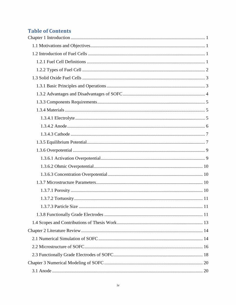
operation temperature, catalyst, fuel gases, charge carriers, and cell efficiency are listed in Table
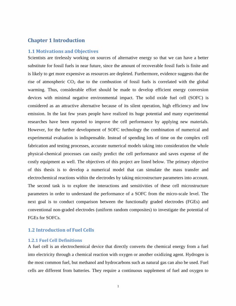
1. The reaction mechanisms of 5 types of fuel cells are provided in Figure 1 (1).
Table 1 Fuel cell types
PEMFC PAFC AFC MCFC SOFC
Electrolyte Polymer
membrane
Liquid H3PO4
Liquid KOH
Molten
carbonate Ceramic
Operating
Temperature
150-180°F
(65-85°C)
370-410°F
(190-210°C)
190-500°F
(90-260°C)
1200-1300°F
(650-700°C)
1350-1850°F
(750-1000°C)
Catalyst Platinum Platinum Platinum Electrode
Material
Electrode
Material
Fuel H2, methanol H2 H2 H2, CO H2, CH4, CO
Charge Carrier H+ H
+ OH
- CO3
2- O
2-
Efficiency 25%-35% 35%-45% 32%-40% 40%-50% 45%-55%
3
Figure 1 Reaction mechanism of different types of fuel cells
1.3 Solid Oxide Fuel Cells
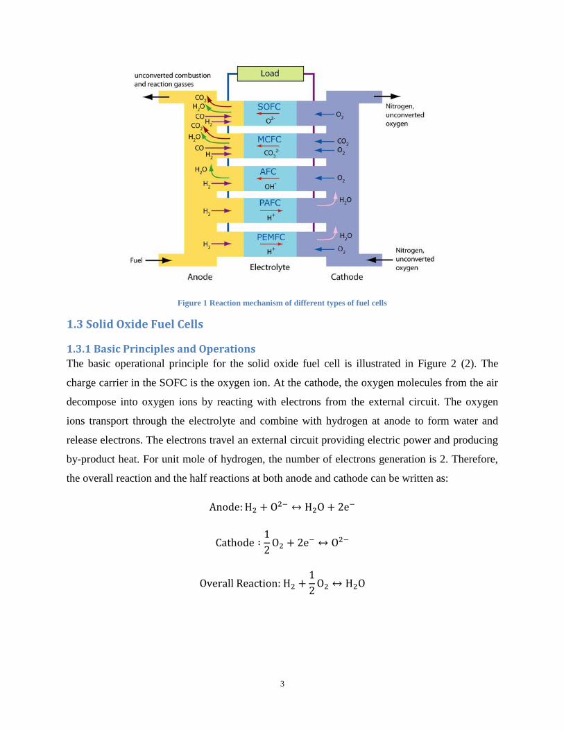
1.3.1 Basic Principles and Operations
The basic operational principle for the solid oxide fuel cell is illustrated in Figure 2 (2). The
charge carrier in the SOFC is the oxygen ion. At the cathode, the oxygen molecules from the air
decompose into oxygen ions by reacting with electrons from the external circuit. The oxygen
ions transport through the electrolyte and combine with hydrogen at anode to form water and
release electrons. The electrons travel an external circuit providing electric power and producing
by-product heat. For unit mole of hydrogen, the number of electrons generation is 2. Therefore,
the overall reaction and the half reactions at both anode and cathode can be written as:

4
Figure 2 Schematics of SOFC
1.3.2 Advantages and Disadvantages of SOFC
The SOFC stands out as a promising technology because it has a number of advantages. First of
all, SOFCs offers very high-energy conversion efficiency as compared with conventional fossil
fuel. Second, the solid component structure will make it simpler to design and manufacture.
Since the reaction zone at the electrode-electrolyte interface becomes a gas-solid contact,
complex electrolyte management is not required. Also, the problems of electrolyte such as
material depletion, lifetime, and the server corrosion of the cell are avoided completely if
compared with liquid-based electrolyte such as PAFC and AFC. Next, because SOFCs are
operated at high-temperature conditions, the relevant electrochemical kinetics at the electrodes
proceeds sufficiently fast without the need of noble metals as catalysts. Furthermore, such high
operating temperatures also make it possible for the internal reforming of methane and other
hydrocarbons to produce hydrogen gas and carbon monoxide. Therefore, SOFCs have a better
ability to allow flexible fuel choices in the reactant gas streams. Finally, the high-temperature
SOFC operation provides a high-quality waste heat for co-generation applications such as heat
engines.
On the other hand, the solid oxide fuel cell has its drawbacks, as well. The challenges include
stack hardware, sealing, and cell interconnects issues due to high operating temperatures. The
high operating temperature also makes materials requirements, mechanical issues, reliability
concerns, and thermal expansion matching tasks more difficult.

5
1.3.3 Components Requirements
Each of the components of an SOFC: anode, cathode and electrolyte must be thermally,
chemically, and mechanically stable at the operating conditions. In addition to those
requirements, the individual layers have additional microstructure, property, and processing
target requirements, as summarized in Table 2. (3)
Table 2 Microstructure, Property, and Processing Requirements of SOFC
Anode Electrolyte Cathode
Microstructure
Porous, many triple-
phase boundaries, stable
to sintering.
Dense, thin, free of cracks
and pinholes
Porous, many triple-
phase boundaries,
stable to sintering.
Electrical
Electronically and
preferably ionically
conductive.
Ionically but not
electronically conductive.
Electronically and
preferably ionically
conductive.
Chemical
Stable in fuel
atmosphere; preferably
also stable in air for
redox tolerance.
Catalytic for oxidation
and reforming but not for
carbon deposition
Stable in both oxidizing and
reducing environments.
Minimal reduction and
resulting electronic
conductivity in reducing
conditions.
Stable in air
environments.
Catalytic for oxygen
reduction. Resistant to
performance loss
caused by chromium
deposition.
Thermal
Expansion
Compatible with other
layers, especially
electrolyte
Compatible with other
layers especially structural
support layers.
Compatible with other
layers, especially
electrolyte
Chemical
Compatibility
Minimal reactivity with
electrolyte and
interconnect
Minimal reactivity with
anode and cathode
Minimal reactivity
with electrolyte and
interconnect
1.3.4 Materials
1.3.4.1 Electrolyte
The electrolyte materials for SOFCs are generally oxygen ion conductors, in which current flow
occurs by the movement of oxygen ions through the crystal lattice. This movement is a result of
thermally activated hopping of the oxygen ion, moving from one crystal lattice to its neighbor
site. To achieve this movement, the crystal must contain unoccupied sites equivalent to those
occupied by the lattice oxygen ions. Yttria-stabilized zirconia (YSZ) is the common electrolyte
materials for SOFCs. YSZ is created by doping ZrO2 with a certain percentage Y2O3. The doping
concentration is typically around 8 mol% because it has been reported (4) that the ion
conductivity reaches peak at that yttria content. In the crystal structure two zirconium cations

6
(Zr4+
) are replaced by two yttrium cations (Y3+
), thus one oxygen site (O2-
) will be left vacant to
maintain charge balance. The vacancy production can also be expressed by Kroger-Vink notation.
→
1.3.4.2 Anode
The most common SOFC anode material is Ni-YSZ cermet, since Ni-YSZ cermet materials meet
most of the electrode requirements aforementioned. In a porous Ni-YSZ cermet anode, the Ni
metal provides the required electronic conductivity and catalytic activity, while the relatively low
thermal expansion of YSZ ceramic prevents Ni from coarsening. In addition, YSZ also provides
ionic conductivity to the electrode, thus effectively broadening the triple phase boundary (TPB).
The electrical conductivity is strongly dependent on the Ni composition. Fig. 3 (5) shows the
conductivity as a function of nickel measured at 1000 °C for different sintering temperatures of
the Ni/ZrO2 (Y2O3) cermet. The percolation threshold plays an important role in the conductivity
of composite materials. Percolation threshold of a SOFC means the critical configuration of same
type of particles connecting with each other to form a bridge through the electrodes. It relies on
composition, porosity, particle sizes and other physical parameters of electrode. In this particular
case, the percolation threshold for nickel (which drives the electronic conductivity) is at
approximately 30 volume percent. Below the threshold, the cermet exhibits predominantly ionic
conduction behavior. Above this threshold, the electrical conductivity increases by about three
orders of magnitude. Moreover, it can be found from Fig. 3 that higher sintering temperature, in
the range given, will result in higher conductivity. In general, the anode and electrolyte are co-
sintered in the range of 1300°C and 1400°C to achieve a dense electrolyte while maintaining an
anode with about 30% porosity. (6)

7
Figure 3 Variation of electrical conductivity
1.3.4.3 Cathode
SOFC cathodes must provide high activity for the electrochemical reduction of oxygen. In order
to maximize the number of TPB sites, SOFC cathodes must provide both ionic and electronic
conductivity, as well as catalytic activity. Because metal conductors are typically not stable in
high temperature oxidizing environments, SOFC cathodes are almost always purely ceramic. In
YSZ-based SOFCs, the dominant cathode material is strontium-doped lanthanum manganite
(LSM) with the general formula La1-xSrxMnO3, where x describes the doping level and is usually
in the range of 10-20% (7) (8). It has a high electronic conductivity, crucial for reducing the
ohmic polarization, especially when the cathode is made thick to provide the structure support.
This material also has proper catalytic properties and maintains mechanical and chemical
stability under high temperature operating conditions. Unfortunately, oxygen-ion conductivity is
very low in LSM. Therefore, LSM-based cathodes are typically mixed with YSZ to form a LSM-
YSZ composite cathode, where the YSZ can provide high ionic conductivity in order to possess
mixed electronic and ionic conductivity and expand the reaction zone.
1.3.5 Equilibrium Potential
The maximum possible electrical energy output and the corresponding electrical potential
difference between the cathode and anode are achieved when a fuel cell is operated under the
thermodynamically equilibrium condition. This maximum possible cell potential is called

8
equilibrium cell potential, or reversible potential. Combing the first and second law of
thermodynamics with Gibbs free energy, we have:
∑ (
)
∑( )
(1.1)
Where is electrical work; z is the number of charges transferred in the reaction per unit
fuel gas, (for SOFC, z=2); F is the Faraday constant (96485 C/mol); is equilibrium potential
of the cell; is the stoichiometric coefficient of the ith
constituent, is the Gibbs free energy
(J/mol) of ith
constituent and the superscript 0 means at standard conditions for temperature and
pressure (STP), which are 25°C (298K) and 1 atm (101325Pa).
The reversible voltage can be approximately calculated as a function of temperature using the
Gibbs free energy and entropy under STP condition. (9)
( )
( ) (1.2)
Where ∑ ( ) ∑ (
) , which is the entropy difference of the chemical
reaction at STP condition; is the standard temperature (298K); and T is the operating
temperature (K). For all of the fuel cell reactions is negative, thus fuel cell reversible
potential will drop due to increasing of temperature. The reversible cell voltage can also be
directly calculated by using the Gibbs free energy of each component at operating temperature,
and can be written as
( )
∑ [ ( )] ∑ [ ( )]
(1.3)
Also from the Gibbs energy expression above, the variation of the reversible cell voltage can be
written in terms of to the pressure change of fuel and oxidant gases, as given below
∏
∏
(1.4)
Where R is the ideal gas law constant (8.314 J/mol·K); is partial pressure (atm) of species i.
The full expression describing how the reversible voltage of SOFC varies with temperature and
pressure can be written as
9
( )
( )
( )
( )
( )
( )
( )
( )
(1.5)
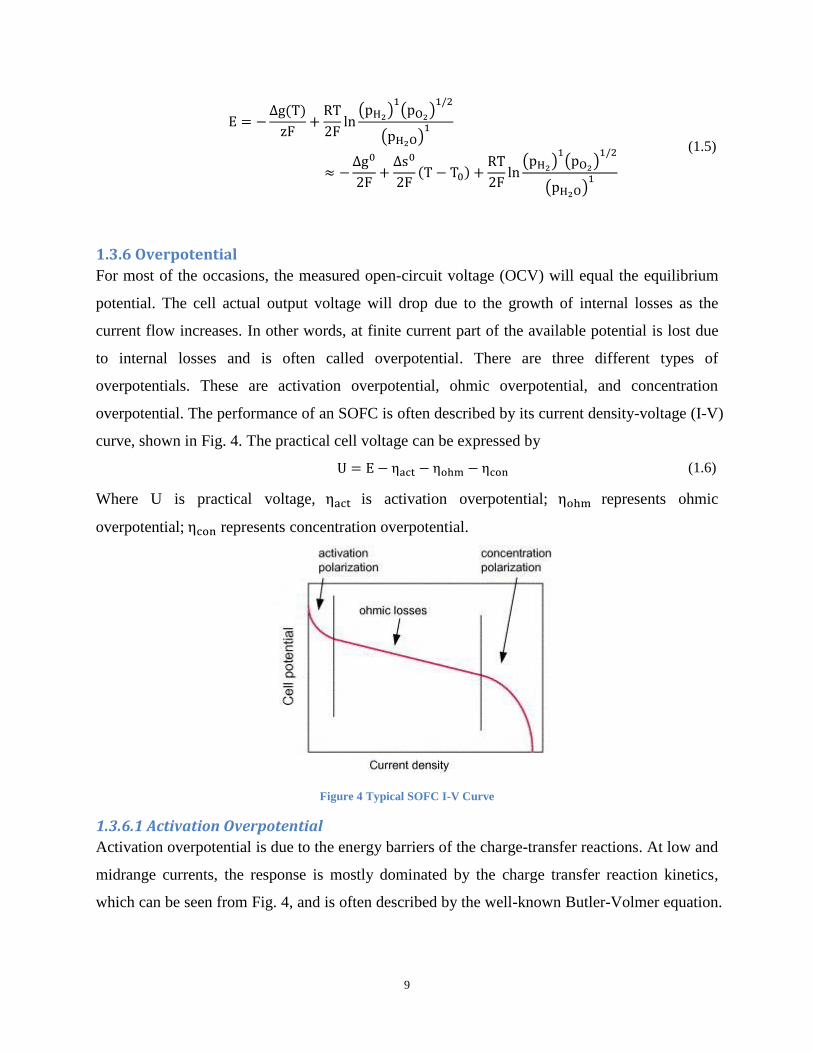
1.3.6 Overpotential
For most of the occasions, the measured open-circuit voltage (OCV) will equal the equilibrium
potential. The cell actual output voltage will drop due to the growth of internal losses as the
current flow increases. In other words, at finite current part of the available potential is lost due
to internal losses and is often called overpotential. There are three different types of
overpotentials. These are activation overpotential, ohmic overpotential, and concentration
overpotential. The performance of an SOFC is often described by its current density-voltage (I-V)
curve, shown in Fig. 4. The practical cell voltage can be expressed by
(1.6)
Where U is practical voltage, is activation overpotential; represents ohmic
overpotential; represents concentration overpotential.
Figure 4 Typical SOFC I-V Curve
1.3.6.1 Activation Overpotential
Activation overpotential is due to the energy barriers of the charge-transfer reactions. At low and
midrange currents, the response is mostly dominated by the charge transfer reaction kinetics,
which can be seen from Fig. 4, and is often described by the well-known Butler-Volmer equation.
10
1.3.6.2 Ohmic Overpotential
Ohmic overpotential is associated with ion transport through the electrolyte and electron transfer
through the electrodes, which is normally solved by Ohm’s law. In Fig. 4, a linear central region
is often attributed to ohmic resistance and the slope is the summation of the electrodes and
electrolyte ohmic resistance.
1.3.6.3 Concentration Overpotential
Concentration overpotential is caused by non-reacting mass transport process in the gas-diffusion
region of the electrodes. As shown in Fig. 4, the effect of this type of loss is most pronounced at
the high current region, where a limiting or maximum current occurs. Concentration
overpotential is important because it defines the maximum current achievable from the device
and it is strongly dependent on the concentration of fuel gas and reactant at fuel channel and
electrode-electrolyte (EE) interface. In other words, it is driven by the gas diffusion process.
Theoretically, the limiting current density occurs when the concentration of fuel gas drops to
zero at EE interface. The mathematical expression of concentration overpotential is listed below
[(
∏
∏ )
( ∏
∏ )
] (1.7)
1.3.7 Microstructure Parameters
1.3.7.1 Porosity
Porosity (ε) is a parameter that measures the void part of the material and can be expressed by a
fraction of the volume of voids over the total volume. According to the definition a large
porosity value means more vacant space in the structure. The range of porosity is between 0 and
1, or as a percentage between 0 and 100%. Porosity value is vital to SOFC performance. For a
low porosity, the number of particles will increase to occupy the empty spots with decreasing
porosity, which in turn causes the available reaction sites near TPB region to increase
considerably. The disadvantage of low porosity is that fewer channels are available for the gas to
transport through the electrodes and hence block the diffusion process. On the other hand, if the
porosity is too high, the electrode will suffer from poor particle connectivity, poor percolation,
and thus poor electrochemical performance. However, large porosity will benefit the gas
diffusion by providing more unobstructed channels. Therefore, it is a trade-off and the porosity
11
range of SOFC is usually between 30% - 70%. (10) The measurement of porosity can be
achieved by applying Archimedes’ method. (11) Basically, a dry weight ( ), saturated weight
( ), and wet weight ( ) of a fuel cell sample need to be measured and the porosity can be
calculated using the eqn. (1.8).
(1.8)
1.3.7.2 Tortuosity
Tortuosity is a property used in porous media describing how the porous structure is twisted. The
definition of tortuosity (τ) can be expressed by eqn. (1.9) and it is always greater or equal to 1. In
a SOFC the higher that number is, the longer the distance that the reactant gas has to travel
before it reaches the TPB region. Therefore, in order to improve diffusion efficiency, tortuosity
needs to be retained as small as possible.
(1.9)
1.3.7.3 Particle Size
Particle size, also called grain size, refers to the diameter of individual “spherical” particles that
can be used to represent the grain structure of an SOFC electrode. Obviously, the conductors in
the electrodes of SOFC are not perfect spherical shapes. Still, it is valid and reasonable
assumption. Currently, particle radius of SOFC electrodes ranging from 0.03 to 10.0 m have
been reported (12). The overpotential drops with decreasing particle size due to the expansion of
reactive surface area. However, if the particle keeps reducing, eventually electrodes will become
dense and block the mass transfer of gases and increase the resistance, increasing the overall
overpotential.
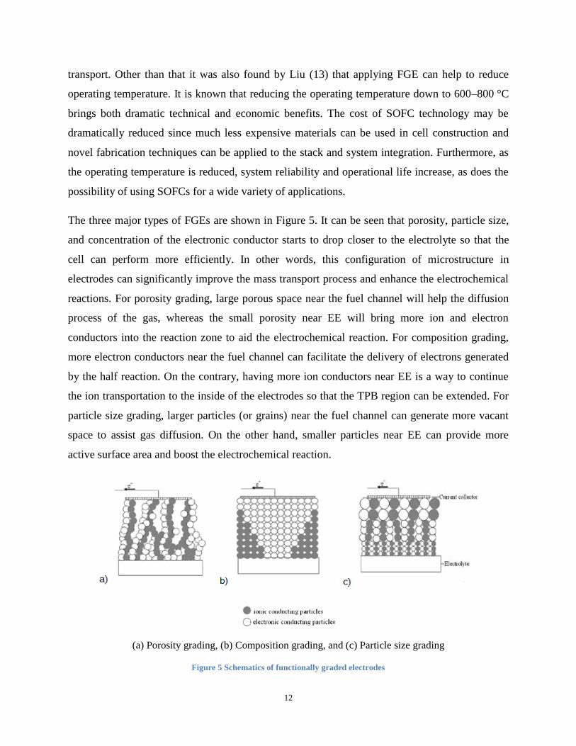
1.3.8 Functionally Grade Electrodes
FGE have been applied to SOFCs in recent years aiming to improve the cell performance by
altering the microstructure including porosity, particle size, and composition of electronic and
ionic conductors near the TPB region. The advantages of FGEs include expanding the
electrochemical reaction area, optimizing the electrical/ionic conductivity, and improving the gas
12
transport. Other than that it was also found by Liu (13) that applying FGE can help to reduce
operating temperature. It is known that reducing the operating temperature down to 600–800 °C
brings both dramatic technical and economic benefits. The cost of SOFC technology may be
dramatically reduced since much less expensive materials can be used in cell construction and
novel fabrication techniques can be applied to the stack and system integration. Furthermore, as
the operating temperature is reduced, system reliability and operational life increase, as does the
possibility of using SOFCs for a wide variety of applications.
The three major types of FGEs are shown in Figure 5. It can be seen that porosity, particle size,
and concentration of the electronic conductor starts to drop closer to the electrolyte so that the
cell can perform more efficiently. In other words, this configuration of microstructure in
electrodes can significantly improve the mass transport process and enhance the electrochemical
reactions. For porosity grading, large porous space near the fuel channel will help the diffusion
process of the gas, whereas the small porosity near EE will bring more ion and electron
conductors into the reaction zone to aid the electrochemical reaction. For composition grading,
more electron conductors near the fuel channel can facilitate the delivery of electrons generated
by the half reaction. On the contrary, having more ion conductors near EE is a way to continue
the ion transportation to the inside of the electrodes so that the TPB region can be extended. For
particle size grading, larger particles (or grains) near the fuel channel can generate more vacant
space to assist gas diffusion. On the other hand, smaller particles near EE can provide more
active surface area and boost the electrochemical reaction.
(a) Porosity grading, (b) Composition grading, and (c) Particle size grading
Figure 5 Schematics of functionally graded electrodes

13
1.4 Scopes and Contributions of Thesis Work A comprehensive numerical model taking consideration of microstructure parameters of SOFC
will be implemented to study the cell performance from a micro-scale. In additional to that, we
will take one step further to explore and establish firm relationships and assumptions the for the
definition of the physical and microstructure parameters of the fuel cell in order to produce
predictions of real cell performance. Furthermore, in order to determine if the numerical model
and sub model correlations of microstructure parameters have the potential to accurately describe
the mass transfer and electrochemical reactions of the cell, model validation will be carried out.
If the numerical results and experimental data show reasonable agreement, the model can be
considered as a proper assumption to resemble the experimental study of SOFC. We can take
advantages of that and perform sensitivity study for all the physical and microstructure
parameters. For the parameters with noticeable sensitivity, they should be highlighted and noted
for accurate measurement during experimental analysis. In contrast, for the parameters with
trivial sensitivity the significance may be neglected and perhaps conventional values may be
used in the analysis. In the end, a sensitivity table of each parameter will be provided so that
model users can make their own judgment on which error range is affordable to them and then
determine if the measurement is necessary for that particular parameter. Another goal of our
research is to modify our adapted numerical model so that it can be applied in more complicated
scenarios, such as FGEs. After that, a detailed analysis of FGEs will be examined and compared
with uniform composite electrodes. The purpose is to find out under which circumstances
applying FGEs will be necessary and can provide better performance. The numerical results need
to be reasonable and represent physics as well. That is to say, by taking sub-model correlations
into account, micro structural parameters will not be treated separately during the grading
process. In contract, as one factor changes, the affected factors will alter correspondingly.
Multiple approaches of grading will also be tested and the one that can improve SOFC
performance most will be determined.

14
Chapter 2 Literature Review
2.1 Numerical Simulation of SOFC
In order to investigate SOFCs mathematically, efforts have been put into development of models
including mass transportation and electrochemical reactions. Zhu et al. (14) presents a new
computational modeling framework for SOFC simulation that takes the whole system including
flow channels and planar membrane-electrode assemblies into consideration. SOFCs can be
operated with a variety of fuels, such as hydrogen, carbon monoxide, hydrocarbons, and
mixtures of those. His work employed multistep reaction mechanisms in terms of detailed
elementary heterogeneous chemical kinetics so that hydrocarbons could be treated as fuel input,
in addition to pure hydrogen. Mass diffusion is calculated by using the dusty-gas model. Detailed
charge transfer reactions are analyzed by separating the mechanism into several elementary steps,
with activation overpotential being determined by the dominating single rate-limiting step.
Won Yong Lee (15) extended Zhu’s study and predicted the activation overpotential of SOFC by
proposing two rate-limiting reactions with a switch-over mechanism. Instead of using only one
rate-limiting reaction, the author claims that two rate-limiting reactions with a switch-over
mechanism is in accordance with actual observations and is also helpful to simulate cell
performance, especially near the limiting current density region.
Regarding mass transport, Suwanwarangkul et al. (16) implement and compare three different
numerical models inside a porous SOFC anode. It was found that current density, reactant
concentration, and pore size are the three key factors in selecting the appropriate mass transport
model. The dusty gas model is considered to be the best approximation for describing mass
transport, especially for multicomponent systems, small porosity, high current density, and low
fuel gas concentrations. However, this model does not have an analytical solution. Therefore, an
iterative approach is required to solve for the solution. Fick’s and Stefan-Maxwell models are
easily to solve but can be applied in fewer occasions because they are restricted to the fuel gas
system, current density region, and so on.
Since the main purpose of this project is to investigate the performances of FGEs in SOFCs by
taking the micro structural parameters into account, a comprehensive mathematical model needs
to be explored and implemented. Chan and Xia (17) proposed a numerical modeling approach to

15
simulate the polarization effects of SOFCs. Their model takes into account electronic, ionic, and
gas transport together with the electrochemical reaction. They can predict the distributions of
overpotentials, current densities, and gas concentrations along the electrodes. The reason Chan
and Xia’s (17) model was selected to be the basis of the study is that their model is built based on
the first principles and includes all the micro structural factors that are critical to the cell
performances. This model can simulate the complex gas transport phenomena in electrodes and
electrochemical reactions at TPB region. The disadvantage of this model is that it can only be
used in uniform electrodes, i.e. fixed micro structural parameters such as porosity, particle size,
and electronic/ ionic composition throughout the whole electrodes. Therefore, the model will be
modified and revised so that it can be applied for both uniform electrodes and FGEs.
Several other numerical models were studied in the literature review, however they all have their
drawbacks and did not fit the goal of this project. For example, in the M. Ni el al. (10) model,
they applied Graham’s law to predict the relationships between the water flux and hydrogen flux.
Graham’s Law states that the flux ratio of two substances is inverse proportional to their molar
masses. And it may not be a reasonable assumption in this case because the flux of the reactant
and product need to obey mass conservation (i.e., flux of water coming out of the electrode
equals to the flux of hydrogen going in). Furthermore, their model was applied to study the FGEs
as well. But all the micro structural parameters are treated separately. For instance, when they try
to perform the porosity grading, particle size of electronic and ionic conductors and tortuosity
stay the same through electrodes. However, physically all those parameters are observed to
correlate with each other. Once one factor changes, the rest of the factors should alter
correspondingly.
In some other CFD-based models such as Wilson Chiu et al. (18) and Huayang Zhu et al. (14),
the activation overpotential is directly calculated by the Butler-Volmer equation and do not take
the micro structural characteristics into consideration. Theoretically, these micro structural
factors are critical to the size of active reaction surface sites and hence affect the rate of
electrochemical reaction. Therefore, these simulations may not fully mimic the electrochemical
reaction process and result in inaccurate prediction. Chan and Xia’s (17) adopt a binary random
packing sphere model created by Costamagna (19) and Bouvard (20) to solve this problem so
that the microstructure parameters can be taken into account when calculating the activation
16
overpotential. Bouvard and Lange used a numerical simulation of the random packing of
particles to study the percolation within a powder mixture (20). Costamagna et al. extended the
theory to propose a model for active area per unit volume (19). In the random packing sphere
model, the electrode is assumed to be a random packing of spheres. By applying coordination
number model together with percolation theory, this model guarantees that the same type of
particles touch each other and form a network or particle chain through the electrode. That is to
say, for any given combination of compositions and particle size ratios of electronic and ionic
conductors, the coordination model is used to differentiate if it is above the percolation threshold
and hence determine if the simulation can be proceeded or not. In other words, if the percolation
threshold is not satisfied, the model will stop the simulation due to the extremely poor
connectivity of particles. As abovementioned, active surface area is supposed to be taking micro
structural parameters into account in order to control the rate of electrochemical reaction. In the
random packing model, the active surface area formula takes all these micro scale factors such as
porosity, particle size, number fraction of electronic and ionic conductors into consideration.
Therefore, charge transfer processes in the TPB can be properly described. Other than activation
overpotential, both ohmic overpotential and concentration overpotential in the electrodes are
affected by micro structural parameters. In a porous structure, the resistivity of electronic/ionic
conductors is called effective resistivity and it depends on porosity, tortuosity and volume
fraction of electronic/ionic conductors of the electrodes. Concentration overpotential is related to
mass transport. Effective diffusion coefficients capture the effects of micro structural parameters
such as porosity, tortuosity and particle size. Our selected model will capture all these
overpotentials from a micro scale level.
2.2 Microstructure of SOFC The primary focus of our study is to investigate how the micro structural parameters are related
to each other. During the literature review, it was determined that for most numerical simulations
which took microstructure into account, the micro structural parameters were assumed to be
some commonly used values. Most of them were neither obtained from experimental data nor
had theory to back them up. This basically meant that all these parameters became tuning factors
which were manipulated to allow the mathematical results to be consistent with experimental
data. In order to improve the applicability of the mathematical model, our goal was to develop
correlations between the micro structural parameters. The correlations are selected based on
17
experimental study including tortuosity/porosity relationships and porosity/particle size ratio
relationships.
Perhaps the most intuitive and straightforward definition of tortuosity is the ratio of the length of
true flow paths to the shortest length between any two points within the pore space. Notice that
by this definition, it is evident that tortuosity is dependent on the microscopic geometry of the
pores. It has been reported that the measurement of tortuosity has been made by both performing
experiments and using mathematical derivation. Recent studies of SOFC using focused ion beam
scanning electron microscopy (FIB-SEM), X-ray computed tomography and gas counter-
diffusion provide evidence that the tortuosity for a typical anode, in an anode-supported cell is
1.33-4.0 (21) (22) (23). On the other hand, many modern SOFC models calculated the value of
the tortuosity in the range of 2 to 17. (24) (25)
Several tortuosity and porosity relations were developed and organized by Cussler (26).
( ) (2.1)
( ) ( ) (2.2)
( ) ( ) (2.3)
( ) [ ( )] (2.4)
where n is an adjustable parameter. Eqn. (2.1) was proposed for the electric tortuosity by Jiang et
al. (27). Eqn. (2.2) (with n = 1/2) was found in a theoretical study on diffusivity of a model
porous system composed of freely overlapping spheres by Matyka et al. (28). The same relation
(with n ≈ 0.86 and n ≈ 1.66) was also reported in measurements of the hydraulic tortuosity for
fixed beds of parallelepiped particles by Archie (29). Weissberg (30) measured the tortuosity in
fixed beds and determined that n is dependent on the particle shape. Eqn. (2.3) is an empirical
relation found for sandy (n = 2) or clay-silt (n = 3) sediments by Comiti et al. (31). Eqn. (2.4),

18
with n = 32/9π ≈ 1.1, was obtained in a model of the diffusive tortuosity in marine mud (the
particles are assumed to be disks) by (32).
Regarding the correlation between particle size and porosity, it has been found that the porosity
has nothing to do with particle size for mono-sized particle and it only relies on the packing type
(33). It has been reported that the electrochemical performance of the cell was extensively
improved when the size of the constituent particles was reduced so as to yield a denser
microstructure (34). In binary mixture of spherical particles, porosity is dependent on
composition of two species and particle size ratio. German (33) finds out that the larger the
particle size ratio is, the higher the packing density at all compositions will be. Conventional
non-graded electrodes and two types of FGEs, namely, particle size graded and porosity graded
SOFC anodes, were compared to evaluate the potential of the SOFC by M. Ni et al. (10). Their
research shows that the particle size graded electrode causes a high reduction in overpotential
from that of the non-graded electrode. Besides, the graded electrode can also increase the active
surface area per unit volume and allow the fuel gas to remain at a high concentration at the
reaction sites. Ricardo Dias (35) explored the dependence of packing porosity on particle size
ratio, but he focused on exploring the extreme limits of the particle size ratio. However, for
common SOFCs, the particle size ratio of electronic and ionic conductors is more or less the
same. S. Yerazunis (36) performed experiments to analyze this particular situation. In the
experiment, the particles sizes are assumed to be comparable. In addition, dense-packed particles
will ensure good connection of particles as it will reduce the path length of the fuel gases and
allow the flow to reach the TPB faster. Based on the experimental data, the curve fitting equation
of the measured data gives the correlation between particle size ratio and porosity.
A number of numerical and experimental studies have been conducted to improve the cell
performance. However to the best of the author’s knowledge, to carry out a mathematical study
by considering the correlations of microstructure parameters has not yet been attempted.
2.3 Functionally Grade Electrodes of SOFC New materials and fabrication techniques have been used in FGEs in order to enhance the
performance of SOFCs. Hart et al. (37) used slurry spraying techniques to observe the cell
performance by setting up electrode layers with different materials. It was found that as
temperature decreases, the functionally layered cell still maintained a high level of performance.

19
Zha et al. (38) fabricated a four-layer cathode and the results indicated the cell performance was
strongly dependent on sintering temperature and oxygen partial pressure. Liu et al. (13) found
out that a functionally graded cathode fabricated by combustion CVD process can dramatically
increase the rates of electrode reactions, enhance the transport of oxygen molecules to the active
reaction sites, and significantly improve the compatibility between the electrodes and other cell
components. As a result, extremely low interfacial polarization resistances and high power
densities have been achieved at operating temperatures of 600-850°C. Efforts have also been
made by examining the advantages of applying FGEs in SOFCs from a mathematical perspective.
Ni et al. (10) developed a mathematical model to compare the uniform composite electrodes with
two types of FGEs (particle size grading and porosity grading) in the anode. Both particle size
and porosity were linearly varied from the flow channel to the electrolyte surface. The results
show that applying FGEs reduced the mass transport resistance and increase the active surface
area near the TPB region, thus improving cell performance. Greene et al. (18) developed
computational model to explore mass transport and ohmic loss in graded SOFC electrodes from a
micro-scale level. A porosity-tortuosity graded electrode is applied to demonstrate the reduction
of ohmic overpotential. Gas fuel concentration and molar flux increases significantly at
electrolyte surface for graded electrodes, so mass transfer is also improved as compared to a
uniform pore structure. Activation overpotential is not calculated based on microstructure
parameters, porosity or tortuosity, as author assumes electrochemical reactions only take place at
electrode-electrolyte surface, where a very thin layer with few microstructure parameters get
involved in the reactions. Thus, it is assumed that the activation overpotential may not be
affected by the grading. Wang et al. (39) implemented a mathematical model to predict SOFCs
performance of electrodes with one interlayer. It was found that in most cases, using an
interlayer in the anode can improve the SOFC performance by reducing the overpotential.
However, for the addition of an interlayer to the cathode, the improvement may vary depending
on the thickness.

20
Chapter 3 Numerical Modeling of SOFC In this chapter we will present a framework for the numerical simulation of SOFCs. This is a
physically based, predictive, quantitative model that can be used for SOFC design and
optimization at the cell level.
3.1 Anode
3.1.1 Overpotential due to electrochemical reactions and ohmic resistance
The overall charge balance relationship can be written as (17):
(3.1)
and are the current density (A/m2) due to transport of electronic and ionic conductors in
anode; is active surface area per unit volume (m2/m
3) of the porous hydrogen electrode; is
the transfer current density per unit area of reactive surface (A/m2). This equation essentially
accounts for the electrochemical reaction rate of the fuel cell along the anode.
The transfer current density is normally described by the general form of the Butler-Volmer (B-
V) equation.
{ (
)
( ( )
)} (3.2)
Where is the exchange current density of anode (A/m2); is the molar fraction of .
is
the molar fraction of at fuel channel. is the charge transfer coefficient and is normally
chosen to be 0.5 for “symmetric” reactions (9).
Applying Ohm’s law for the electronic and ionic conductors, we get:
(3.3)
is the effective resistivity (Ω·m) of the anode electronic conductors;
is the effective
resistivity of anode ionic conductors; and are electronic and ionic potential (V), respectively.
The effective resistivity can be determined by (40):
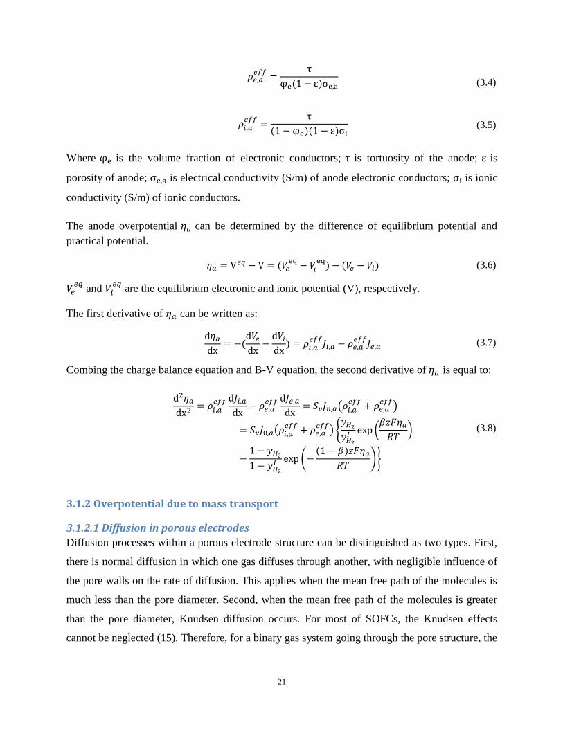
21
( )
(3.4)
( )( ) (3.5)
Where is the volume fraction of electronic conductors; is tortuosity of the anode; is
porosity of anode; is electrical conductivity (S/m) of anode electronic conductors; is ionic
conductivity (S/m) of ionic conductors.
The anode overpotential can be determined by the difference of equilibrium potential and
practical potential.
(
) ( ) (3.6)
and
are the equilibrium electronic and ionic potential (V), respectively.
The first derivative of can be written as:
( )
(3.7)
Combing the charge balance equation and B-V equation, the second derivative of is equal to:
(
)
(
) { (
)
( ( )
)}
(3.8)
3.1.2 Overpotential due to mass transport
3.1.2.1 Diffusion in porous electrodes
Diffusion processes within a porous electrode structure can be distinguished as two types. First,
there is normal diffusion in which one gas diffuses through another, with negligible influence of
the pore walls on the rate of diffusion. This applies when the mean free path of the molecules is
much less than the pore diameter. Second, when the mean free path of the molecules is greater
than the pore diameter, Knudsen diffusion occurs. For most of SOFCs, the Knudsen effects
cannot be neglected (15). Therefore, for a binary gas system going through the pore structure, the
22
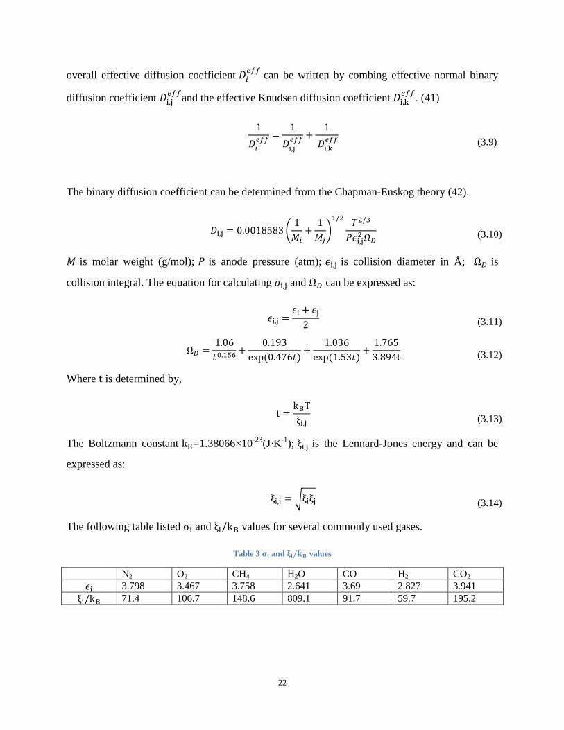
overall effective diffusion coefficient
can be written by combing effective normal binary
diffusion coefficient
and the effective Knudsen diffusion coefficient
. (41)
(3.9)
The binary diffusion coefficient can be determined from the Chapman-Enskog theory (42).
(
)
(3.10)
is molar weight (g/mol); is anode pressure (atm); is collision diameter in Å; is
collision integral. The equation for calculating and can be expressed as:
(3.11)
( )
( )
(3.12)
Where is determined by,
(3.13)
The Boltzmann constant =1.38066×10⁻²³
(J·K-1
); is the Lennard-Jones energy and can be
expressed as:
√ (3.14)
The following table listed and values for several commonly used gases.
Table 3 and values
N2 O2 CH4 H2O CO H2 CO2
3.798 3.467 3.758 2.641 3.69 2.827 3.941
71.4 106.7 148.6 809.1 91.7 59.7 195.2
23
The effectively diffusion coefficient depends on the microstructure of the porous anode,
quantified through the porosity and tortuosity values. Thus, the effective binary diffusion
coefficient can be written as: (17)
(3.15)
For Knudsen diffusion, its coefficient can be described as (14),
√
(3.16)
is the pore diameter (m) and is assumed to be approximately equal to the hydraulic diameter.
(43)
(3.17)
is specific surface area based on the solid volume. For random packing of binary, is
expressed as:
( )
( )
(3.18)
is the diameter (m) of electronic particles, is number fraction of electronic particles,
.
Similarly as with the effective binary diffusion coefficient, the effective Knudsen diffusion
coefficient can be expressed as:
(3.19)
3.1.2.2 Fick’s Law
Fick’s Law is the simplest form to describe the mass transfer through the porous media. The
general form of the model takes into account both diffusion and convection mass transfer and
can be expressed as: (15) (16)

24
(3.20)
Where is molar flux (mol/m2·s) of species i;
is the effective diffusion coefficient (m
2/s)
of specie i; is the concentration (mol/m3) of specie i; v is the convection velocity (m/s); p is
pressure (Pa); is the permeability (m2); is the viscosity of mixture (kg / m·s).
The equations of diffusion for both H2 and H2O are listed as follows: (44)
(3.21)
(3.22)
The convection velocity is due to inertia. Under constant operating temperature, the ideal gas law
can be written as:
(3.23)
If pressure is uniform throughout the electrode, then is constant. According to eqn. (3.23),
will also be constant. Then we will have:
(3.24)
For equimolar counter-current mass transfer, . The summation of eqn. (3.21) and
(3.22) will give us:
(
)
( ) (3.25)
Eqn. (3.25) can be rearranged as:
(3.26)
Substitute above equation back into H2 and H2O flux equations, which are eqn. (3.21) and eqn.
(3.22), we have:
25
(
)
(
)
(3.27)
(
)
(
)
(3.28)
According to flux and current density relations as well as ideal gas law,
(3.29)
(3.30)
Eqn. (3.27) turns into:
( )
(3.31)
3.1.2.3 Dusty Gas Model
The Dusty Gas Model (DGM) (16) is another commonly used diffusion model. It is assumes that
the pore walls consist of giant molecules (dust) uniformly distributed in space. These dust
molecules are considered to be dummy, pseudo, species in the mixture. The general form of the
DGM is shown as
∑
(
) (3.32)

26
The first term on the left hand side (LHS) expresses Knudsen diffusion. The second term
indicates the multi-component diffusion and is described by the Stefan-Maxwell Model. The first
term on the right hand side (RHS) denotes the concentration gradient along the electrode The
second term takes into consideration the effect of total pressure gradient on mass transport. If we
assume pressure is uniform along the entire electrode, then this term drops out. The DGM
reduces to:
∑
(3.33)
For a H2 - H2O binary system, the DGM can be rewritten as:
(3.34)
Under steady state, and . The above equation turns into:
(
)
(3.35)
Then hydrogen flux can be expressed as:
(3.36)
This above equation is exactly the same as Fick’s Model if the pressure term is neglected.
3.1.3 Anode governing equations and boundary conditions
In our simulation, the Fick’s model is selected to calculate the mass transfer over anode.
Combining with the electrochemical reaction formulas, we get a total of three governing
equations. They are:
27
(
) { (
)
( ( )
)}
(3.37)
{ (
)
( ( )
)}
(3.38)
( )
(3.39)
The boundary conditions for the governing equations can be derived as follows: At the fuel gas
inlet, which is also the location of the current collector, the hydrogen molar fraction is equal to
the bulk flow value. The total current density only comes from the transport of electrons. As a
result, the boundary conditions can be expressed as:
| ( ) | |
|
(3.40)
Since the governing equation associated with solving for the overpotential is a second order
partial differential equation, another boundary condition is required. At the electrode-electrolyte
(EE) interface, the transport of ions is the only factor that contributes to the overall current
density. Therefore, ion current density equals to the overall current density. This allows for the
boundary condition of the overpotential to be from defined, as in eqn. (3.7).
| |
(3.41)
After solving the governing equations, , and distribution can be obtained. Then the
overall overpotential of the anode can be written as follows. At the fuel gas inlet,
28
| ( ) ( | ) (3.42)
At the electrode-electrolyte interface,
| ( ) ( | ) (3.43)
Adding the above two equations together, we will get anode overall overpotential:
|
| |
(
) ( | | )
(3.44)
3.2 Cathode
3.2.1 Overpotential due to electrochemical reactions and ohmic resistance
The electrochemical reaction equations in cathode are similar to the ones in anode and can be
derived in a similar fashion, to produce the following.
(
) { (
) ( ( )
)}
(3.45)
{ (
) ( ( )
)} (3.46)
Where is cathode overpotential; is cathode exchange current density;
is effective
resistivity of cathode electronic conductors. is the current density due to transport of
electronic current conductors in cathode.
3.2.2 Overpotential due to mass transport
3.2.2.1 Fick’s Law
The model is proposed by Berger (44). An effective Knudsen diffusion coefficient of O2 can be
defined by
( )
(3.47)
29
The effective normal diffusion of oxygen taking both conduction and convection transport can be
defined by
( )
( )
(3.48)
Total concentration of O2 is equal to the summation of Knudsen concentration and normal
concentration.
( )
( )
(
)
(3.49)
On the cathode side, nitrogen does not involve any electrochemical reaction, so flux of nitrogen
at steady state is zero. Then we have . The above equation turns into
(
) (
) (3.50)
The O2 flux becomes
(
)
(3.51)
3.2.2.2 Dusty Gas Model
Assume pressure is uniform throughout cathode, and then the DGM equation becomes
(3.52)

30
Because and , DGM equation becomes
( )
(3.53)
Rearranging the above equation, we have
(
)
(3.54)
It can be found that the DGM and Fick’s Law have the same formula in this case.
According to flux and current density relations as well as ideal gas law, we have
(3.55)
(3.56)
Then eqn. (3.57) becomes
(
)
(3.57)
3.2.3 Cathode governing equations and boundary conditions
Similarly as anode, three coupled governing equations for cathode can be listed as
(
) { (
) ( ( )
)} (3.58)
{ (
) ( ( )
)} (3.59)
(
)
(3.60)
31
At fuel gas inlet, which is also the location of current collector, the oxygen molar fraction is
equal to the bulk flow value and the total current density only comes from the transport of
electrons. The boundary conditions can then be expressed as:
|
( ) | | |
(3.61)
On electrode-electrolyte (EE) interface, the transport of ions will be the only factor contributes to
the overall current density. Thus, the treatment of overpotential on the EE boundary can be
obtained as follows.
| |
(3.62)
After solving the governing equations, the cathode overall overpotential can be calculated as:
|
| |
(
) ( | | )
(3.63)
3.3 Electrolyte The overpotential from the electrolyte can be simply expressed by the Ohm’s Law.
(3.64)
The area specific resistance (Ω·m2) equals to . L is the thickness of electrolyte (m) and
is the ionic conductivity (S·m-1
) of electrolyte.
3.4 Numerical Solution Procedure The numerical domain for anode is listed below.
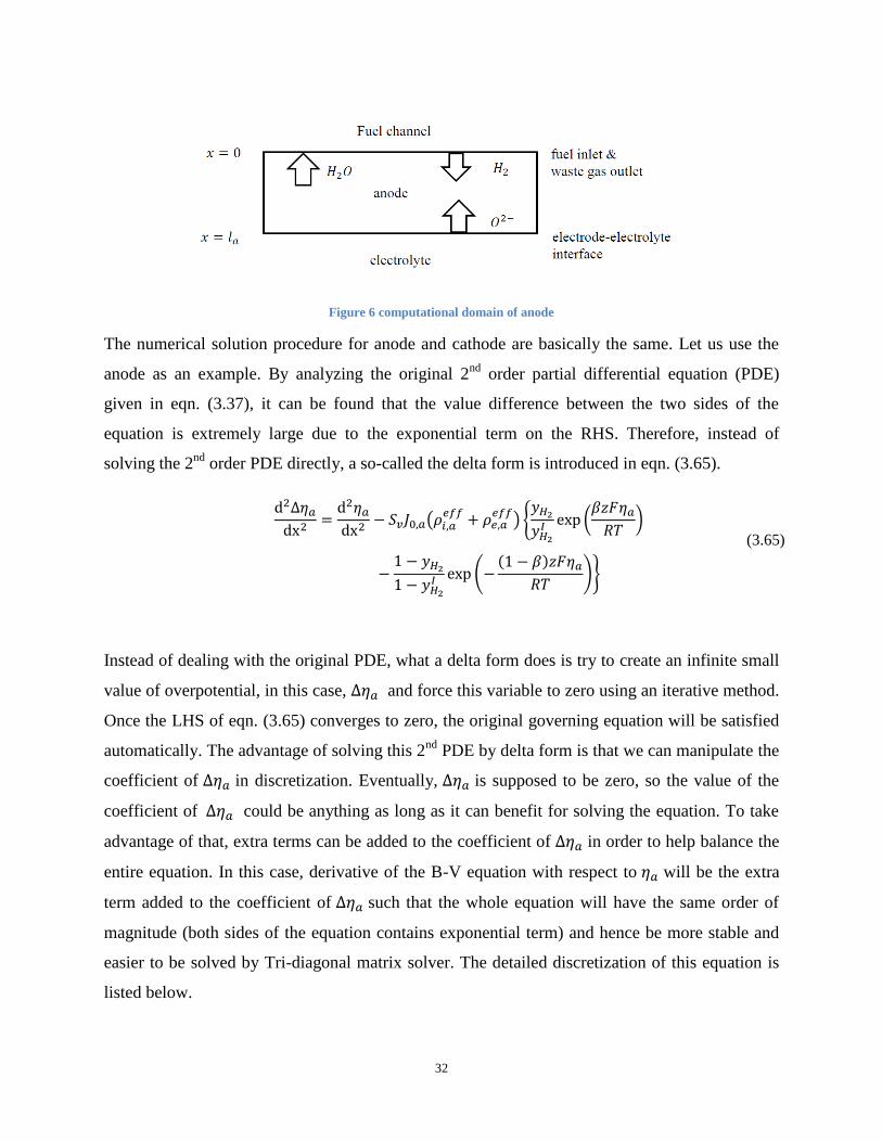
32
Figure 6 computational domain of anode
The numerical solution procedure for anode and cathode are basically the same. Let us use the
anode as an example. By analyzing the original 2nd
order partial differential equation (PDE)
given in eqn. (3.37), it can be found that the value difference between the two sides of the
equation is extremely large due to the exponential term on the RHS. Therefore, instead of
solving the 2nd
order PDE directly, a so-called the delta form is introduced in eqn. (3.65).
(
) { (
)
( ( )
)}
(3.65)
Instead of dealing with the original PDE, what a delta form does is try to create an infinite small
value of overpotential, in this case, and force this variable to zero using an iterative method.
Once the LHS of eqn. (3.65) converges to zero, the original governing equation will be satisfied
automatically. The advantage of solving this 2nd
PDE by delta form is that we can manipulate the
coefficient of in discretization. Eventually, is supposed to be zero, so the value of the
coefficient of could be anything as long as it can benefit for solving the equation. To take
advantage of that, extra terms can be added to the coefficient of in order to help balance the
entire equation. In this case, derivative of the B-V equation with respect to will be the extra
term added to the coefficient of such that the whole equation will have the same order of
magnitude (both sides of the equation contains exponential term) and hence be more stable and
easier to be solved by Tri-diagonal matrix solver. The detailed discretization of this equation is
listed below.
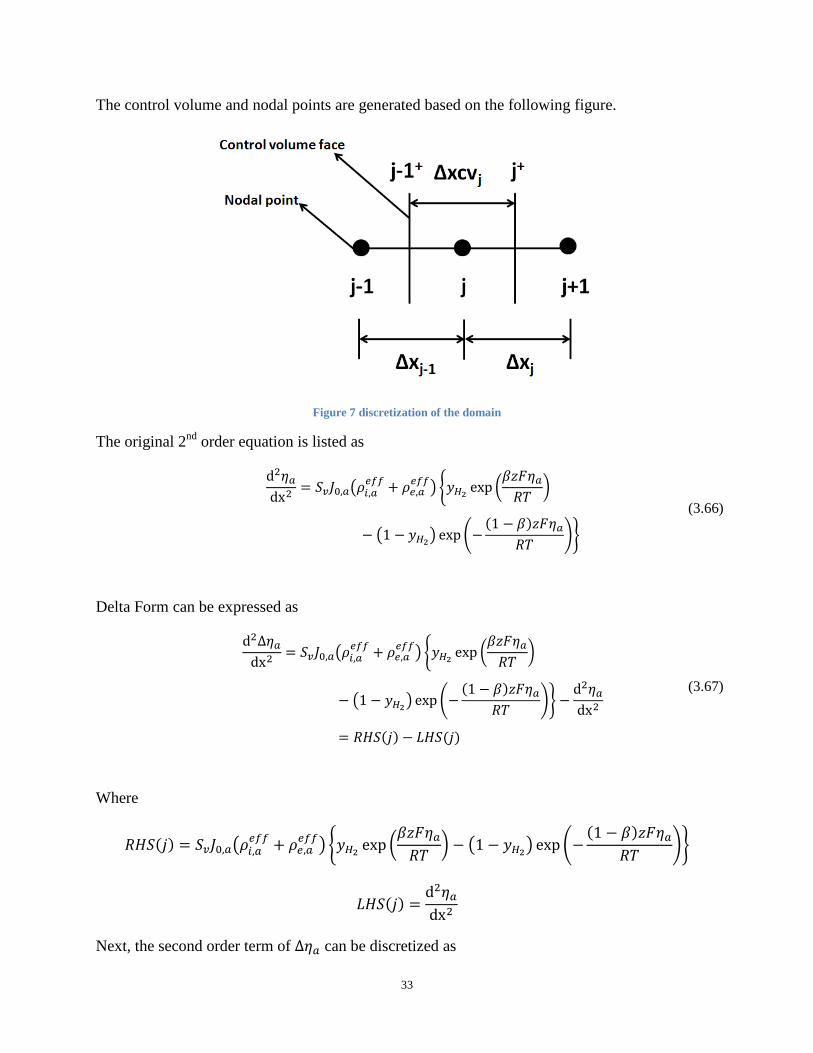
33
The control volume and nodal points are generated based on the following figure.
Figure 7 discretization of the domain
The original 2nd
order equation is listed as
(
) { (
)
( ) ( ( )
)}
(3.66)
Delta Form can be expressed as
(
) { (
)
( ) ( ( )
)}
( ) ( )
(3.67)
Where
( ) (
) { (
) ( ) ( ( )
)}
( )
Next, the second order term of can be discretized as
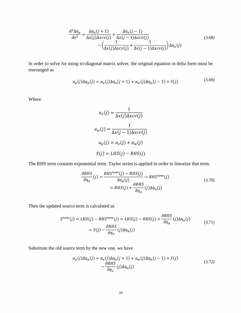
34
( )
( ) ( )
( )
( ) ( )
(
( ) ( )
( ) ( )) ( )
(3.68)
In order to solve for using tri-diagonal matrix solver, the original equation in delta form must be
rearranged as
( ) ( ) ( ) ( ) ( ) ( ) ( ) (3.69)
Where
( )
( ) ( )
( )
( ) ( )
( ) ( ) ( )
( ) ( ) ( )
The RHS term contains exponential term. Taylor series is applied in order to linearize that term.
( )
( ) ( )
( ) ( )
( )
( ) ( )
(3.70)
Then the updated source term is calculated as
( ) ( ) ( ) ( ) ( )
( ) ( )
( )
( ) ( )
(3.71)
Substitute the old source term by the new one, we have
( ) ( ) ( ) ( ) ( ) ( ) ( )
( ) ( )
(3.72)
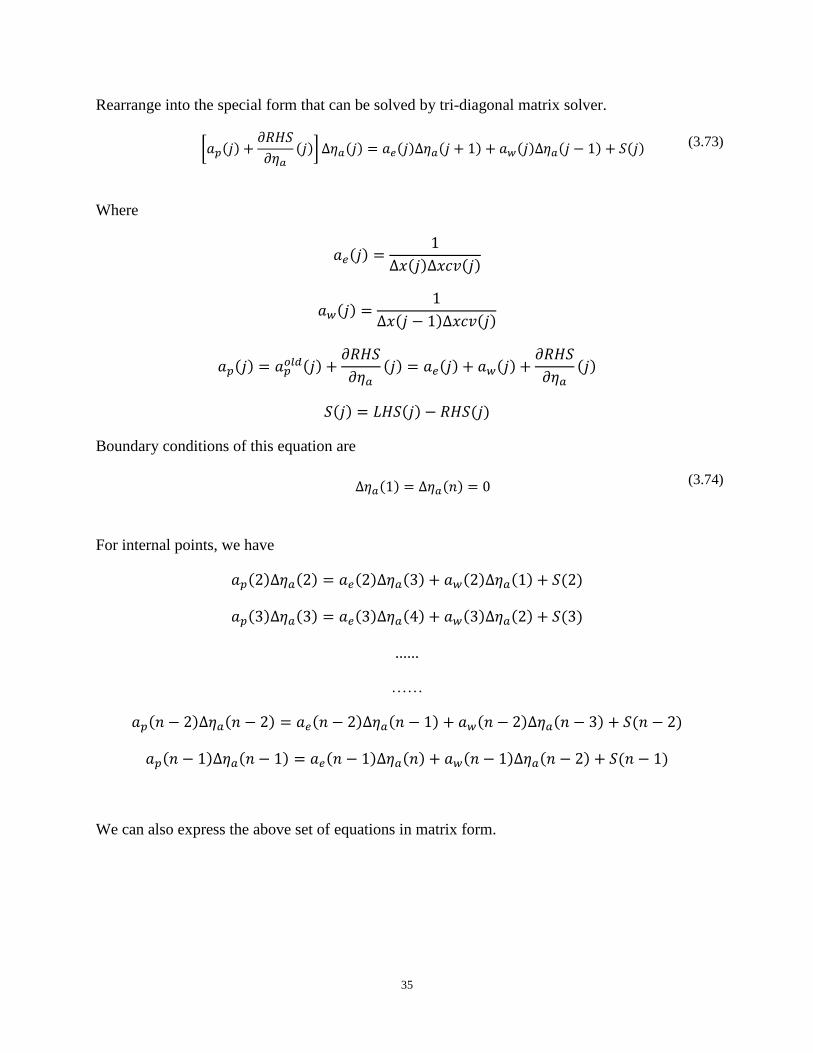
35
Rearrange into the special form that can be solved by tri-diagonal matrix solver.
[ ( )
( )] ( ) ( ) ( ) ( ) ( ) ( )
(3.73)
Where
( )
( ) ( )
( )
( ) ( )
( ) ( )
( ) ( ) ( )
( )
( ) ( ) ( )
Boundary conditions of this equation are
( ) ( ) (3.74)
For internal points, we have
( ) ( ) ( ) ( ) ( ) ( ) ( )
( ) ( ) ( ) ( ) ( ) ( ) ( )
......
……
( ) ( ) ( ) ( ) ( ) ( ) ( )
( ) ( ) ( ) ( ) ( ) ( ) ( )
We can also express the above set of equations in matrix form.
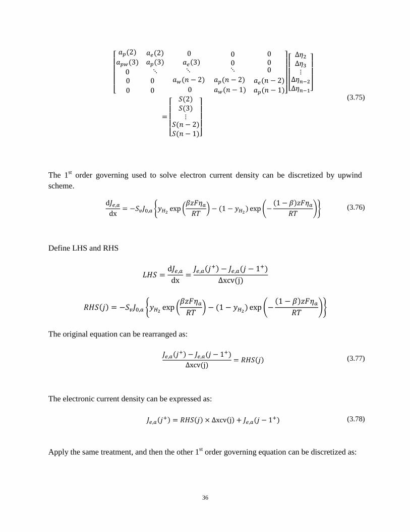
36
[ ( )
( )
( ) ( )
( )
( ) ( ) ( )
( ) ( )]
[
]
[ ( ) ( )
( ) ( )]
(3.75)
The 1st order governing used to solve electron current density can be discretized by upwind
scheme.
{ (
) ( ) ( ( )
)} (3.76)
Define LHS and RHS
(
) ( )
( )
( ) { (
) ( ) ( ( )
)}
The original equation can be rearranged as:
(
) ( )
( ) ( ) (3.77)
The electronic current density can be expressed as:
( ) ( ) ( ) (
) (3.78)
Apply the same treatment, and then the other 1st order governing equation can be discretized as:

37
( )
(3.79)
Define LHS and RHS
( ) ( )
( )
( )
( )
( )
Then, we have
( ) ( )
( ) ( )
(3.80)
Hydrogen concentration can be calculated as:
( ) ( ) ( ) ( ) (3.81)
Along x direction, the domain will be divided into 500 sections. The flow chart show that the
overall numerical treatment of these three coupled governing equations is to bond the 2nd
order
equation with either of the 1st order equations and solve them together until converges. The under
relaxation factor (urf) in this case can be chosen to be 0.5. After that, the third equation is
coupled and all the governing equations are iterated together. Please notice that if all three
equations are solved simultaneously, the code may end up not converging unless applying a
heavy under-relaxation factor (0<urf<0.1). We want to avoid this because it will make the
computing process very time-consuming.

38
Figure 8 Flow chart
39
Chapter 4 Analysis of model parameters In order to produce predictions of real cell performance, firm relationships and assumptions need
to be established for the definition of the physical and microstructure parameters of the fuel cell.
These assumptions and relationships are defined in this chapter.
4.1 Active surface area per unit volume The active surface area per unit volume of a composite, porous material cannot be simply
calculated on the basis of the properties of the pure materials or porosity/tortuosity parameters,
alone. Instead, the composite material can be represented as randomly packed spheres, as was
done by Costamagna and Bouvard (19) (20). They utilized the particle coordination number
together with percolation theory to build a model of a porous, composite electrode. This model
ensures good pathways for both electrical and ionic conduction by connecting the particles of the
same type together and forming a bridge through the electrode.
The following equations describe the number of contact points on one electronic or ionic particle
(4.1)
(4.2)
(4.3)
(4.4)
Zi-e is the average number of contact points between an electronic conductor particle and other
ionic conductor particles; Zi-i is the average number of contact points between an ionic conductor
particle and other ionic conductor particles; Ze-i is the average number of contact points between
an ionic conductor particle and other electronic conductor particles; Ze-e is the average number of
contact points between an electronic conductor particle and other electronic conductor particles.
Zi is the average number of contacts between both ionic conductor and electronic conductor
particles with an ionic conductor particle; Ze is the average number of contacts of both ionic
conductor and electronic conductor particles with an electronic conductor particle; and Z is the
overall average number of contacts between particles. In addition, ni is the number fraction of
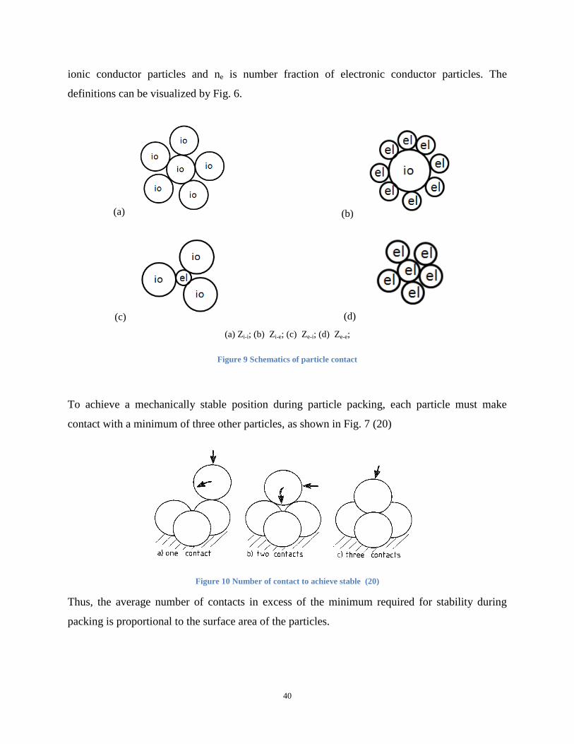
40
ionic conductor particles and ne is number fraction of electronic conductor particles. The
definitions can be visualized by Fig. 6.
(a) (b)
(c) (d)
(a) Zi-i; (b) Zi-e; (c) Ze-i; (d) Ze-e;
Figure 9 Schematics of particle contact
To achieve a mechanically stable position during particle packing, each particle must make
contact with a minimum of three other particles, as shown in Fig. 7 (20)
Figure 10 Number of contact to achieve stable (20)
Thus, the average number of contacts in excess of the minimum required for stability during
packing is proportional to the surface area of the particles.
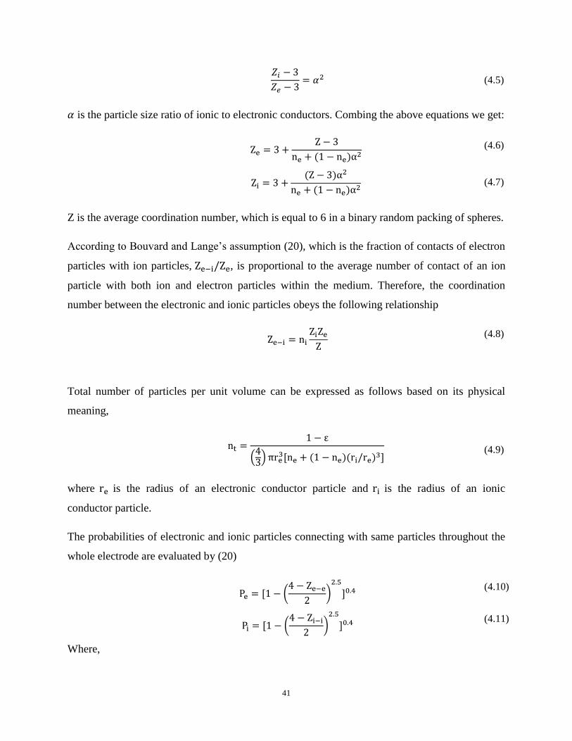
41
(4.5)
is the particle size ratio of ionic to electronic conductors. Combing the above equations we get:
( ) (4.6)
( )
( ) (4.7)
Z is the average coordination number, which is equal to 6 in a binary random packing of spheres.
According to Bouvard and Lange’s assumption (20), which is the fraction of contacts of electron
particles with ion particles, , is proportional to the average number of contact of an ion
particle with both ion and electron particles within the medium. Therefore, the coordination
number between the electronic and ionic particles obeys the following relationship
(4.8)
Total number of particles per unit volume can be expressed as follows based on its physical
meaning,
( )
[ ( )( ) ]
(4.9)
where is the radius of an electronic conductor particle and is the radius of an ionic
conductor particle.
The probabilities of electronic and ionic particles connecting with same particles throughout the
whole electrode are evaluated by (20)
[ (
)
] (4.10)
[ (
)
] (4.11)
Where,
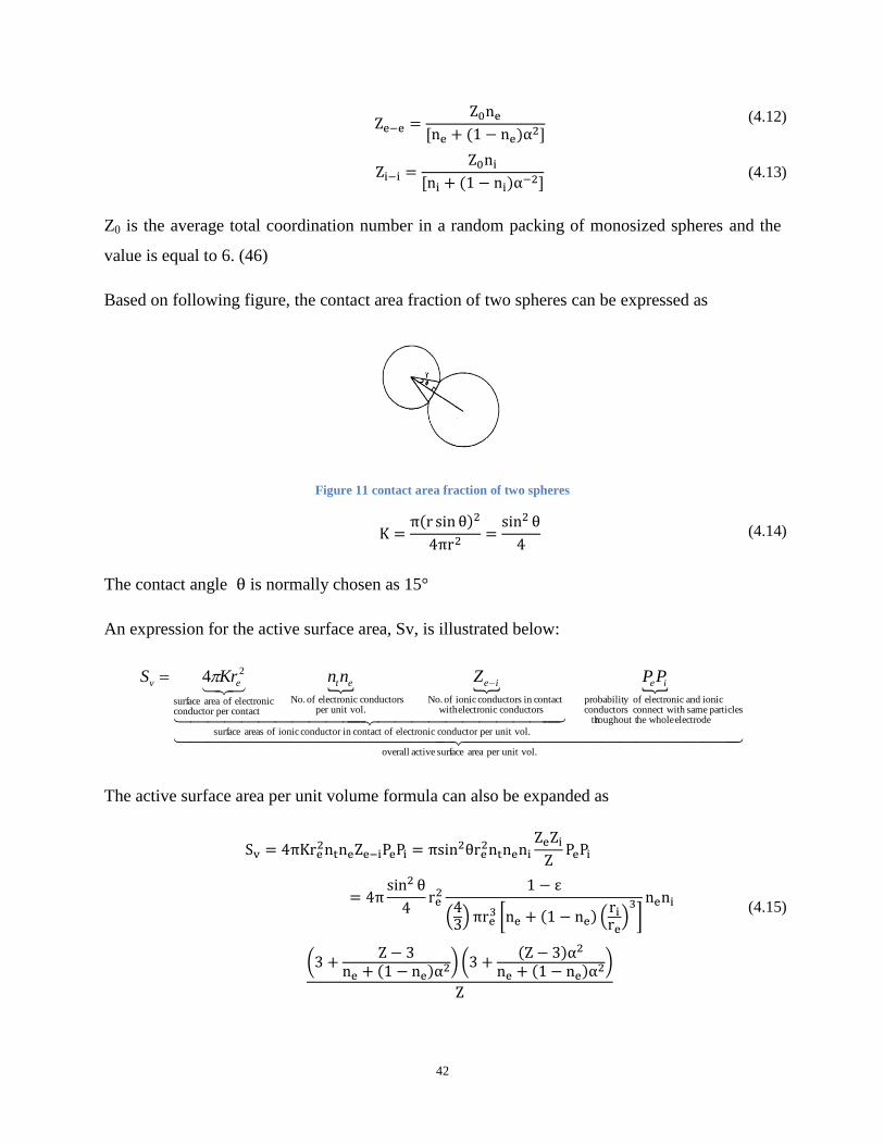
42
[ ( ) ]
(4.12)
[ ( ) ]
(4.13)
Z0 is the average total coordination number in a random packing of monosized spheres and the
value is equal to 6. (46)
Based on following figure, the contact area fraction of two spheres can be expressed as
Figure 11 contact area fraction of two spheres
( )
(4.14)
The contact angle is normally chosen as 15°
An expression for the active surface area, Sv, is illustrated below:
unit vol.per area surface active overall
electrode wholeheroughout t thparticles sameth connect wi conductors
ionic and electronic ofy probabilit
unit vol.per conductor electronic ofcontact in conductor ionic of areas surface
conductors electronic with contact in conductors ionic of No.
unit vol.per conductors electronic of No.
contactper conductor electronic of area surface
24 ieieetev PPZnnKrS
The active surface area per unit volume formula can also be expanded as
( )
[ ( ) ( ) ]
(
( ) ) (
( )
( ) )
(4.15)

43
[
(
[ ( )
]
)
]
[
(
[ ( )
]
)
]
4.2 Exchange current density
Exchange current density can be determined from detailed elementary reactions. (15) (14)
4.2.1 Anode exchange current density
The follow development is summarized from Lee (2001). The anode overall half reaction is
)(2)()()()( 22 NieYSZVgOHYSZOgH O
X
O
The detailed elementary reactions are listed below.
Absorption on the anode surface:
I)(2)(2)(2 NiHNigH
Charge transfer reaction at the triple phase boundary (TPB) region:
III)()()()()(
II)()()()()(
2
2
NieYSZOHNiYSZOHNiH
NieYSZOHNiYSZONiH
Adsorption/desorption on the YSZ surface:
IV)()()( 22 YSZgOHYSZOH
Transfer of the oxygen ion between the surface and the bulk YSZ:
V)()()()( 2 YSZVYSZOYSZYSZO O
X
O
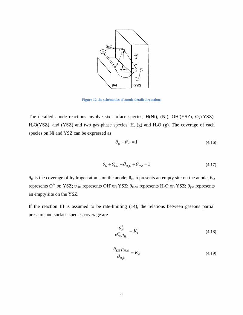
44
Figure 12 the schematics of anode detailed reactions
The detailed anode reactions involve six surface species, H(Ni), (Ni), OH-(YSZ), O2
-(YSZ),
H2O(YSZ), and (YSZ) and two gas-phase species, H2 (g) and H2O (g). The coverage of each
species on Ni and YSZ can be expressed as
1 NiH (4.16)
12
YSZOHOHO (4.17)
θH is the coverage of hydrogen atoms on the anode; θNi represents an empty site on the anode; θO
represents O2-
on YSZ; θOH represents OH- on YSZ; θH2O represents H2O on YSZ; θysz represents
an empty site on the YSZ.
If the reaction III is assumed to be rate-limiting (14), the relations between gaseous partial
pressure and surface species coverage are
12
2
2
KpHNi
H
(4.18)
4
2
2 Kp
OH
OHYSZ
(4.19)

45
5KO
YSZ
(4.20)
is the equilibrium constant of reaction i.
For reaction II, the current density can be written in elementary form as
RT
FVk
RT
FVkFl
JJJ
OHNiHOTPB
a
)1(expexp2 2
2,22
1,2
21
(4.21)
At zero current density (J1=J2), with K2=k2,1/k2,2, the equilibrium electrical potential can be found
as:
RT
FVK
HO
OHNi exp2
(4.22)
The current density is determined by rate-limiting reaction III and can be expressed as:
RT
FVk
RT
FVkFl
JJJ
NiOHOHHTPB
a
)1(expexp2 3
2,33
1,3
21
2
(4.23)
At zero current density (J1=J2=0), with K3=k3,1/k3,2, substitute the surface coverage species
equations, which are eqn. (4.18), eqn. (4.19), eqn. (4.20) and eqn. (4.22) into eqn. (4.23), the
equilibrium electrical potential can be found.
2
2
4321
5ln
2 H
OHeq
pKKKK
pK
F
RTV (4.24)

46
Combining all equations in this section together, the current density can be expressed in terms of
the activation overpotential
RT
F
RT
FJJ aa
aa
)1(exp
)1(exp 33
,0 (4.25)
Where
(4.26)
2/)1(
4321
52/12/1
14
52,3
,03
2
2
2
2
1
2
H
OH
H
OHTPB
a
pKKKK
pKpKK
pKFklJ
(4.27)
Then the anode exchange current density can be simplified by setting =0.5 for the
“symmetric” reactions.
2/1
1
4/34/1
1
,0
2
22
2 1 H
OHH
HapK
ppKJJ
(4.28)
Where
4/3
45
4/1
232,3 )/()(22
KKKKFklJ TPBH (4.29)
The parameter
2HJ is taken here as an empirical parameter that is adjusted to represent
experimentally observed performance. Also, from eqn. (4.29) we know that
2HJ is only a
function of temperature. This indicates that under the same operating temperature
2HJ is a fixed
value.
According to Lapujoulade and Neil’s report (47), reasonable estimate of hydrogen adsorption-
desorption rates are available. K1 can be computed as
47
RT
EA
RTM
S
Kdes
des
H
i
exp
2
2
0
1
2
(4.30)
where the surface site density Γ= 2.6×10⁻⁹
mol/cm2, the pre-exponential factor Ades = 5.59×10
19
s·cm2/mol, and the activation energy Edes = 88.12 kJ/mol, the sticking coefficient S=0.01. It can
be found that K1 is a function of operating temperature.
Exchange current density will normally be obtained by the Electrochemical Impedance
Spectroscopy (EIS) plot from experimental study. EIS plot is captured when the fuel cell is
working at open circuit voltage. This means partial pressures of the fuel gases at TPB region are
equal to the bulk partial pressure during the measurement. Hence,
2HJ can be calculated by
inputting exchange current density, temperature and fuel gas input from eqn. (4.28). Once
2HJ is
obtained, the exchange current density with different fuel gases input under the same operating
temperature can be predicted.
4/3
)(
4/1
)(1
2/1
)(1
,04/34/1
1
2/1
1
,0
22
2
22
2
2)(
)(11
bulkOHbulkH
bulkH
a
OHH
H
aHppTK
pTKJ
ppK
pKJJ
(4.31)
4.2.2 Cathode exchange current density Again, summarizing from Lee (2001), the cathode overall half reaction is:
)()(2)()(2
12 YSZOLSMeYSZVgO X
OO (4.32)
The detailed elementary reactions are listed below:
Adsorption/desorption on LSM surface
VI)(2)(2)(2 LSMOLSMgO ad
Charge transfer reaction at TPB region

48
VII)()()(2)()( LSMYSZOLSMeYSZVLSMO X
OOad
Figure 13 the schematics of cathode detailed reactions
Where )(YSZVO
and )(YSZOX
O denoted the oxygen vacancies and lattice oxygen ions in the bulk
of the electrolyte; )(LSMe is the electron within the cathode; )(LSMOad is adsorbed atomic
oxygen on the cathode surface; )(LSM is an unoccupied cathode surface site. The charge
transfer step is assumed to be rate-limiting, as a result the adsorption-desorption reaction is
equilibrated.
62
2
2 Kp
O
vO
(4.33)
θv represents the coverage of the vacancy on the cathode surface and θO represents the coverage
of adsorbed oxygen on the cathode surface.
The surface of the cathode is covered with only adsorbed oxygen and vacancies.
1 Ov (4.34)
Using above two equations, the surface coverage can be expressed by the gaseous partial
pressure and the equilibrium constant
49
2/12/1
6
2/1
2
2
O
O
OpK
p
(4.35)
2/12/1
6
2/1
6
2O
vpK
K
(4.36)
The current density can be written in elementary form from reaction VII as
RT
FVk
RT
FVkFlJJJ OvTPBc
)1(expexp2 7
2,77
1,721
(4.37)
At zero current density (J1=J2=0), with K7=k7,1/k7,2, substitute the eqn. (4.35) and (4.36) into eqn.
(4.37), the equilibrium electrical potential can be found
7
2/1
6
2/1
02lnKK
p
F
RTV
O
(4.38)
Combining all equations in this section together, the current density can be expressed in terms of
activation overpotential
RT
F
RT
FJJ cc
cc
)1(exp
)1(exp 77
,0 (4.39)
Where
(4.40)
7
2
2
2
1
7
2/1
6
2/1
2/12/1
6
2/1
2,7
,0
2
KK
ppK
pFklJ
O
O
OTPB
c
(4.41)
Then the cathode exchange current density can be simplified by setting =0.5 for “symmetric”
reactions.

50
2/1
6
4/1
6
,0
2
2
2
1
K
p
K
p
JJ
O
O
Oc (4.42)
Where
2/1
2,7
2/1
1,722
kFklJ TPBO
(4.43)
The parameter
2OJ is taken here also as an empirical parameter that is adjusted to represent
experimentally observed performance.
For an LSM-YSZ interface, Matsuzaki and Yasuda (48) presented an Arrhenius expression for
K6 as
RT
EAK
O
O2
2exp6 (4.44)
Where the pre-exponential factor 2OA = 4.9×10
8 atm, and the activation energy
2OE = 200 kJ/mol.
Similar to the anode, cathode exchange current density of different fuel gases input under the
same operating temperature can be predicted by using eqn. (4.42) once
2OJ is known.
4.3 Material conductivity The conductivity of commonly used materials in the anode (nickel), cathode (LSM) and
electrolyte (YSZ) are studied and expressed as only a function of temperature. The purpose is to
make the model compact and reduce the unnecessary inputs.
4.3.1 Electrical conductivity of anode material (nickel) The most commonly used electron conducting material in the anode is nickel. The electrical
conductivity of nickel can be expressed as a function of temperature (49).
( )
( )
( )[ ( )] (4.45)

51
The reference temperature is =20°C; the resistivity of nickel at 20°C, ( ) = 6.99×10⁻⁸
Ω·m.
4.3.2 Electrical conductivity of cathode material (LSM) Lanthanum strontium manganite (LSM) is an oxide ceramic material with the general formula
La1-xSrxMnO3, where x describes the doping level and is usually in the range of 10-20%.
The electrical conductivity of LSM measured at PO2=1 bar is listed as follows (50).
For x≤1/3,
Tk
E
x
xxxx
T B
actce exp
)17(
)1718)(6(108.22
226
, (4.46)
Where eVxEact 00.2)3(59.0 , Bk =8.617×10⁻⁵
eV K−1
.
For x≥1/3,
Tk
Exx
T B
actce exp)1(
108.2 6
, (4.47)
Where eVxEact 16.0)3(036.0 .
The unit of eqn. (4.46) and eqn. (4.47) is in terms of S/cm.
Figure 14 LSM electrical conductivity vs. partial pressure of oxygen (50)

52
Fig. 14 shows the how the electrical conductivity of LSM varies with oxygen partial pressure
(50). It can be determined that the electrical conductivity remains almost unchanged for oxygen
partial pressure in the range -5<log[P(O2)/bar]<0. Or in other words, 0.0067bar<P(O2)<1bar. In
the cathode the most common fuel gas is air or pure oxygen, which means that partial pressure of
oxygen is either 0.21 bar or 1 bar. By observing Fig. 14, it can be concluded that the conductivity
of those different partial pressure keeps almost the same for doping level between 0.1 and 0.2.
To sum up, the electrical condctivity keeps consistent no matter the input is air or pure oxygen.
4.3.3 Ionic conductivity of electrolyte material (YSZ) YSZ ionic conductivity was studied by S.P.S. Badwal (4). In his experiments, the conductivity
was measured by a 4 probe DC technique.
Figure 15 Arrhenius plots for three different Y2O3 doping of ZrO2 compositions
The governing equation of ion conductivity in a crystalline solid electrolyte is given as (9)
RT
ET act
io exp1
0 (4.48)
Where 0 (S·m-1
·K) is pre-exponential coefficient; actE (J/mol) is activation energy.
SOFC operation temperature is usually between 650°C and 900°C. Correspondingly, in the
above Arrhenius plot x-axis is approximately from 8.5 to 10.8. The curve fitting of eqn. (4.48)

53
will give us two unknown variables, which are 0 and actE . For different doping compositions,
those two variables can be calculated as follows by least square method.
For 3 mol% Y2O3,
molJE
KmS
act /102709.8
1047172.2
4
17
0
For 8 mol% Y2O3,
molJE
KmS
act /107605.7
1094550.2
4
17
0
For 12 mol% Y2O3,
molJE
KmS
act /109602.8
1087489.5
4
17
0
By applying the above curve fitting equations, YSZ ion conductivity for different Y2O3 doping
compositions under different temperatures can be obtained as
Table 4 ion conductivity for different doping of Y2O3 at different temperature
YSZ ionic conductivity
(Ω-1
·m-1
)
650°C
700°C
750°C
800°C
850°C
900°C
3 mol% Y2O3 0.558 0.921 1.444 2.167 3.129 4.370
8 mol% Y2O3 1.294 2.064 3.138 4.577 6.441 8.789
12 mol% Y2O3 0.540 0.934 1.527 2.379 3.554 5.122
Next, the YSZ ion conductivity equation depends on both temperature and doping composition
will be discussed. Eqn. (4.49) is the mathematical form.
( ) (4.49)

54
is the desired ion conductivity value (S/m); is temperature (°C); Y is Y2O3 doping
composition (mol %)
The function of is assumed to form a parabolic shape at both T- and Y- plane, thus the
formula is built as
(4.50)
Here are the coefficients that need to be calculated.
The least square algorithm is applied to fit function . Based on Table 4, for each pair of T
(temperature) and Y (Y2O3 doping composition), there is one corresponding ion conductivity
value, g. The purpose is to find one set of that will make ∑ ( )
minimum. In order to
do that, the gradient of ∑ ( )
must be equal to zero.
∑ ( )
(4.51)
After solving the above six equations, the value of each can be calculated.
Then, the expression of conductivity can be expressed as
(4.52)
which is plotted in the 3D contour below.
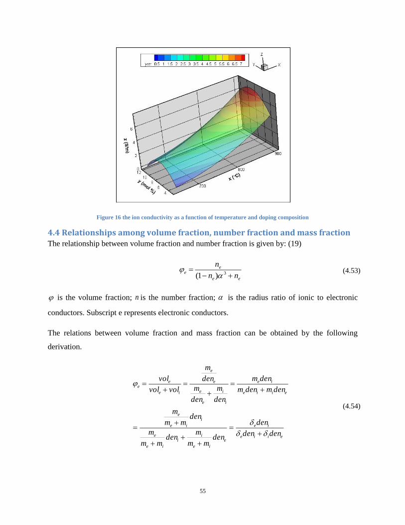
55
Figure 16 the ion conductivity as a function of temperature and doping composition
4.4 Relationships among volume fraction, number fraction and mass fraction
The relationship between volume fraction and number fraction is given by: (19)
ee
ee
nn
n
3)1( (4.53)
is the volume fraction; n is the number fraction; is the radius ratio of ionic to electronic
conductors. Subscript e represents electronic conductors.
The relations between volume fraction and mass fraction can be obtained by the following
derivation.
eiie
ie
e
ie
ii
ie
e
i
ie
e
eiie
ie
i
i
e
e
e
e
ie
ee
denden
den
denmm
mden
mm
m
denmm
m
denmdenm
denm
den
m
den
m
den
m
volvol
vol
(4.54)

56
is volume fraction; vol is volume; m is mass; den is density; is mass fraction. Subscript e
and i represent electronic and ionic conductors, respectively. It can be observed from the
equation that if densities of the two materials are the same, their mass fraction is also identical.
4.5 Relationship between porosity and tortuosity Since the materials in the model are assumed to be composed of binary spherical mixtures, the
model proposed by Ricardo Dias [8] was adopted. His model is consistent with our assumption
of treating the particles to be spheres. The tortuosity () is assumed to be inversely proportional
to porosity (). The adjustable variable (n) in the correlation has been analyzed and determined
so that it will fit most of the fuel cell cases.
(4.55)
The following figure plots the data from the experiments of (51) for sphere mixtures. By
applying eqn. (4.55) as the relationship, it can be observed from Fig. 17 that most of the data
falls in the region where n value is in between 0.4 and 0.5.
Figure 17 Dependence of the tortuosity on the packing porosity
In order to further investigate the adjustable number, Ricardo (35) performed an experimental
study for binary mixture spheres as shown in Fig. 18.

57
Figure 18 Dependence of n on φD for different Dl/ Ds
In the above figure, Dl/ Ds is the diameter ratio of large particle to small particle; D is volume
fraction of large particles. It can be observed that for the particle size ratio less or equal to 3.33,
the value of n is approximately to be 0.5 regardless of the volume fraction. For most of the
SOFCs, the sizes of ionic and electronic conductors are more or less the same, so it is reasonable
to select the value of n to be equal to 0.5 in the numerical model. However, if we happen to
encounter large particle size ratio, the above plot will be used for selecting the appropriate n
value.
4.6 Relationship between porosity and particle size
4.6.1 Relationship between mono-sized sphere particles and porosity
For mono-sized spherical particles, porosity has nothing to do with particle size. It only depends
on the particle packing type. The following table lists porosity values under different particle
packing types.
Table 5 packing type vs. porosity

58
Porosity can also be calculated by the given coordination number. For example, if particles are
packed in a simple unit cubic format, which means one particle is connected with 6 other
particles, the porosity can be calculated as
4764.02
1
3
41
3
(4.56)
Figure 19 simple cubic packing
Another way to express porosity is to use packing density, which is the solid part in the porous
structure, and can be calculated as 1-ε.
4.6.2 Relationship between bimodal mixtures of spherical particles and porosity
For bimodal mixtures of spherical particles, S. Yerazunis (36) performed experimental study and
plotted packing density vs. volume fraction as shown in Fig. 20.
Figure 20 packing density vs. composition for different particle size ratios

59
The curve fitting equation of that experimental study is listed as
L
L
L
sL
L
s
D
D
D
D
1955.0315.0362.01
64.01
247.0
(4.57)
where is volume fraction. The subscript L means large particle size, S means small particle size.
Particle size ratio, number fraction, and porosity are the variables contained in eqn. (4.57). As
long as two of them are provided, the last one can be calculated. This correlation is useful and
can be used practical situations. For example, in the experimental study, once the volume
fraction and particle sizes of electron conducting and ion conducting particles are determined, the
porosity can be calculated using eqn. (4.57) without any measurement needed.
It can be deduced from the experimental data that the porosity value is trying to approach 0.36 as
particle size ratio is getting closer to 1. Therefore, we assume that when ionic particle size is
equal to electronic particle size, the porosity is set to be 0.36. It is obvious that under that
particular circumstance bimodal mixtures turn into mono-sized particles. Table 5 lists the
porosity range for different packing of mono-sized particles, which is from 0.26 to 0.66. The
assumption we made is reasonable because 0.36 falls in between that range.

60
Chapter 5 Model Validation In order to determine if the mathematical model and correlations of microstructure parameters
have the potential to accurately describe the cell performance, model validation needs to be
carried out. Three experiments are selected to facilitate the comparison between mathematical
simulation and experimental data. All the selected experiments have different perspectives on
investigating the cell performance. It will demonstrate a strong compatibility and proper
selection of sub model correlations for our model if there is good agreement between the
mathematical and experimental data.
There will be two types of inputs in the model: operational inputs and physical inputs. The
operational inputs of the model include operating temperature and pressure, fuel gases
composition, and current density. The physical inputs include exchange current density,
thickness of anode, cathode and electrolyte, volume fraction (or mass fraction) of electronic and
ionic conductors, particle size of electronic and ionic conductors, porosity, and tortuosity.
5.1 Case No.1 The first experimental data selected is from S.P. Jiang (52). The objective of the experiment is to
investigate the effect of impregnation of different volume fractions of nano-sized YSZ particles
into nickel anodes on the electrode behavior for the hydrogen oxidation reaction. The following
table lists the parameters provided by the paper.

61
Table 6 values of input parameters used in the model
Parameter (provided by paper) Value
Operating Temperature 1073K
Pressure 1.0 atm
Anode thickness 30μm
Electrolyte thickness 1mm
Gas fuel in anode 97% H2 (3% H2O)
Volume fraction of NiO/YSZ Ni: 100%/0%
Ni+2.7mg/cm2 YSZ: 83%/17%
Ni+4.0mg/cm2 YSZ: 79%/21%
Porosity 30%
YSZ particle size 0.1-0.3 μm
In order to solve this problem using the developed numerical model, Ni particle size, tortuosity,
and anode exchange current density need to be determined.
Let us take Ni+4.0mg/cm2
YSZ for example. The volume fraction of Ni/YSZ for Ni+4.0mg/cm2
YSZ is given as 79%/21%. Combining the eqn. (4.10) - (4.13) from the coordination number
model and volume fraction eqn. (4.53), the upper and lower bounds of particle size ratio and
number fraction can be found in Table 7. The values within the two bounds will maintain the
threshold of the same types of particles (electronic conductors and ionic conductors) connecting
with each other through the electrodes and hence ensure good conductivity.
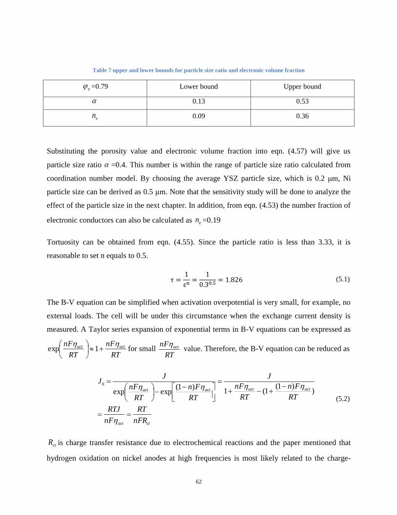
62
Table 7 upper and lower bounds for particle size ratio and electronic volume fraction
e =0.79 Lower bound Upper bound
0.13 0.53
en 0.09 0.36
Substituting the porosity value and electronic volume fraction into eqn. (4.57) will give us
particle size ratio =0.4. This number is within the range of particle size ratio calculated from
coordination number model. By choosing the average YSZ particle size, which is 0.2 μm, Ni
particle size can be derived as 0.5 μm. Note that the sensitivity study will be done to analyze the
effect of the particle size in the next chapter. In addition, from eqn. (4.53) the number fraction of
electronic conductors can also be calculated as en =0.19
Tortuosity can be obtained from eqn. (4.55). Since the particle ratio is less than 3.33, it is
reasonable to set n equals to 0.5.
(5.1)
The B-V equation can be simplified when activation overpotential is very small, for example, no
external loads. The cell will be under this circumstance when the exchange current density is
measured. A Taylor series expansion of exponential terms in B-V equations can be expressed as
RT
nF
RT
nF actact
1exp for small
RT
nF act value. Therefore, the B-V equation can be reduced as
ctact
actactactact
nFR
RT
nF
RTJ
RT
Fn
RT
nF
J
RT
Fn
RT
nF
JJ
)
)1(1(1
)1(expexp
0
(5.2)
ctR is charge transfer resistance due to electrochemical reactions and the paper mentioned that
hydrogen oxidation on nickel anodes at high frequencies is most likely related to the charge-

63
transfer reaction at the TPB region. In contrast to the behavior of the high-frequency arc,
impregnation of nano-YSZ phase has no effect on the characteristic frequency of the low-
frequency arc.
Table 8 Fitted impedance parameters for hydrogen oxidation on Ni-YSZ anodes
Figure 21 Nyquist plot of Ni/YSZ anode at 900°C operating temperature
Therefore, based on Table 8 and Fig. 21 provided by the paper, the anode exchange current
density at 800 °C can be expressed as
2
21
11
,
,0 0651.071.0964852
1073314.8
cmA
cmmolC
KmolKJ
nFR
RTJ
act
a (5.3)
Since all the parameters applied in the model have been calculated, the mathematical simulation
can be performed. From the figure below, it can be seen that the numerical results and
experimental data agree reasonably well with each other.

64
Figure 22 Comparison between numerical results and experimental data
5.2 Case No.2 The second experiment comes from Kim et al (53). The objective of this experiment was to
investigate the performance and durability of Ni-coated YSZ anodes for intermediate
temperature solid oxide fuel cells.

65
Table 9 input parameters in the experiment
Parameter (provided by paper) Value Operating Temperature 700°C / 800°C
Pressure 1.0 atm Anode thickness 1200μm
Electrolyte thickness 7μm
Cathode thickness 30μm
Gas fuel in anode 97% H2 (3% H
2O)
Gas fuel in cathode air
Volume fraction of NiO/YSZ 40%/60%
Mass fraction of LSM/YSZ 50%50%
Porosity 40%
NiO particle size 20-30nm YSZ particle size <300nm
LSM particle size, anode exchange current density, and cathode exchange current density will be
calculated by using the sub model correlation and EIS plot from experimental measurement.
Let me take 700°C case as an example to show the procedure of calculation. The same approach
will be used for the 800°C operating temperature case. Regarding the anode and cathode
exchange current density, they can be figured by the EIS plots as shown in Fig. 23. For common
SOFCs, the low frequency arc will represent the anode charge transfer resistance and high
frequency arc will represent the cathode charge transfer resistance. Therefore, the anode and
cathode exchange current can be approximate as follows.
2
21
11
,
,0 5989.007.0964852
973314.8
cmA
cmmolC
KmolKJ
nFR
RTi
act
a

66
2
21
11
,
,0 1612.026.0964852
973314.8
cmA
cmmolC
KmolKJ
nFR
RTi
cct
c
Figure 23 EIS plots of the SOFC at 700°C and 800°C
In the anode, the porosity is given and the particle size ratio and tortuosity can be calculated by
sub model correlations. It turns out be that the particle size ratio is equal to 0.718 by applying
eqn. (4.57) and this value falls within the upper and lower limits of the coordination number
model. The tortuosity can also be calculated as 1.581 from eqn. (4.55). In cathode, the particle
size ratio and tortuosity can be calculated as 0.71 and 1.581, respectively using the same
approach as the anode.
The anode electron particle size is within 20 to 30 µm based on the information provided by the
paper. Once we know the particle size ratio, the ionic particle, YSZ, can be obtained to be 39 µm
by assuming the Ni particle size to be 25 µm, which is the average of the given bounds. Again
the sensitivity study will be done to analyze the effect of the particle size. In the cathode, the
particle size of LSM can be determined as 27.7 µm by the calculated particle size of YSZ from
anode.
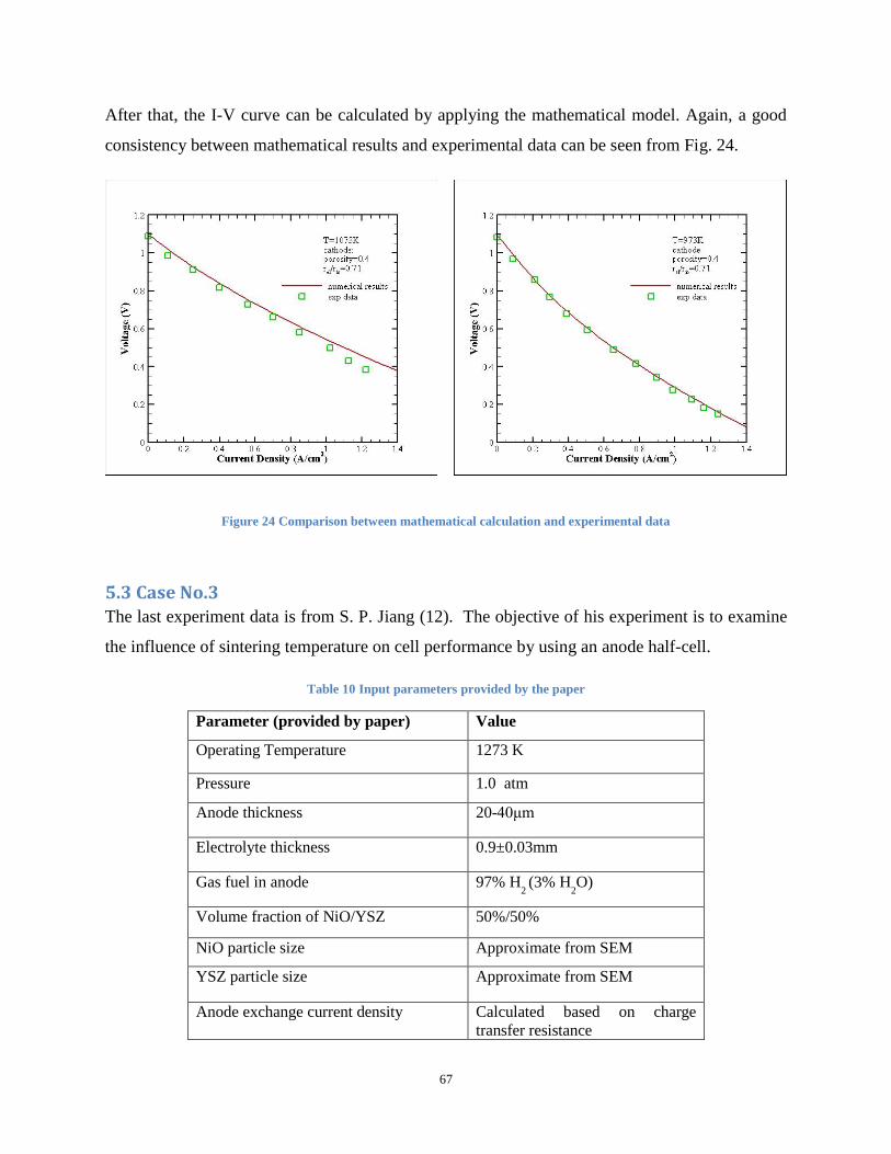
67
After that, the I-V curve can be calculated by applying the mathematical model. Again, a good
consistency between mathematical results and experimental data can be seen from Fig. 24.
Figure 24 Comparison between mathematical calculation and experimental data
5.3 Case No.3 The last experiment data is from S. P. Jiang (12). The objective of his experiment is to examine
the influence of sintering temperature on cell performance by using an anode half-cell.
Table 10 Input parameters provided by the paper
Parameter (provided by paper) Value Operating Temperature 1273 K
Pressure 1.0 atm Anode thickness 20-40μm
Electrolyte thickness 0.9±0.03mm
Gas fuel in anode 97% H2 (3% H
2O)
Volume fraction of NiO/YSZ 50%/50%
NiO particle size Approximate from SEM YSZ particle size Approximate from SEM
Anode exchange current density Calculated based on charge
transfer resistance
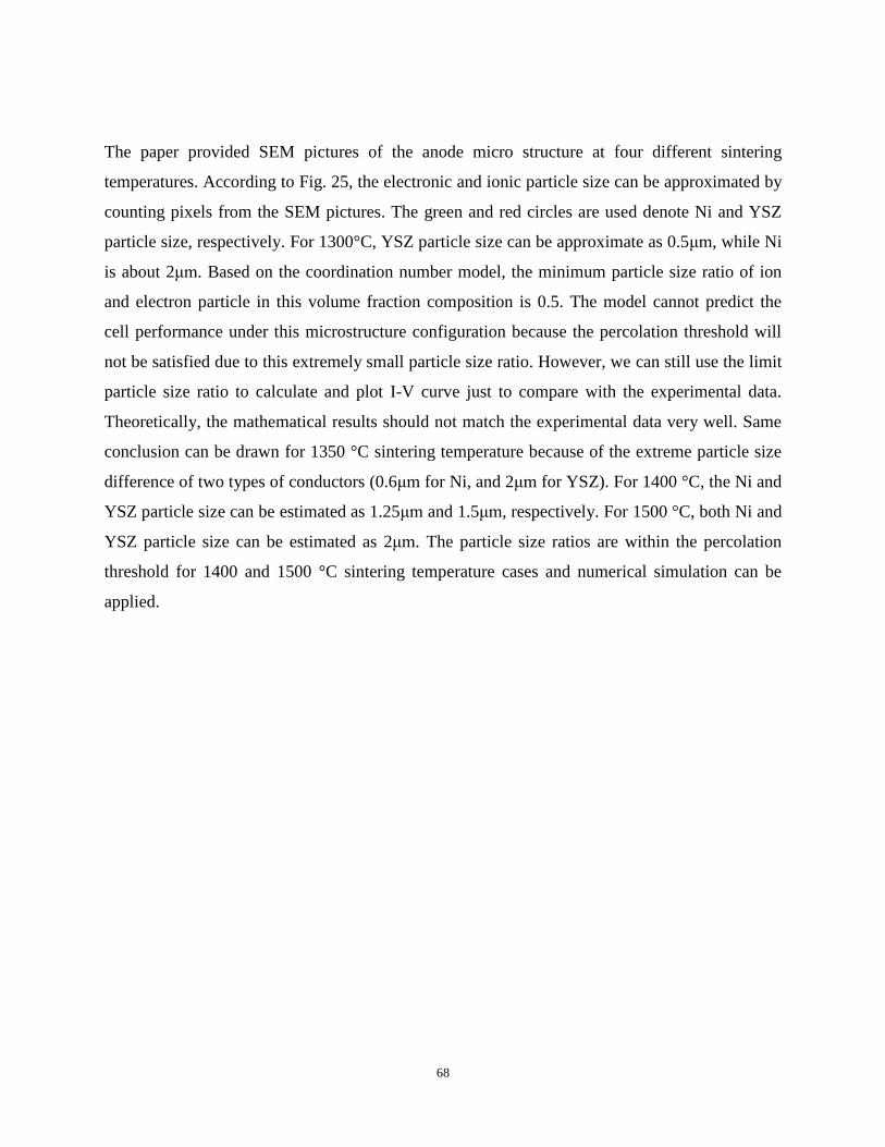
68
The paper provided SEM pictures of the anode micro structure at four different sintering
temperatures. According to Fig. 25, the electronic and ionic particle size can be approximated by
counting pixels from the SEM pictures. The green and red circles are used denote Ni and YSZ
particle size, respectively. For 1300°C, YSZ particle size can be approximate as 0.5μm, while Ni
is about 2μm. Based on the coordination number model, the minimum particle size ratio of ion
and electron particle in this volume fraction composition is 0.5. The model cannot predict the
cell performance under this microstructure configuration because the percolation threshold will
not be satisfied due to this extremely small particle size ratio. However, we can still use the limit
particle size ratio to calculate and plot I-V curve just to compare with the experimental data.
Theoretically, the mathematical results should not match the experimental data very well. Same
conclusion can be drawn for 1350 °C sintering temperature because of the extreme particle size
difference of two types of conductors (0.6μm for Ni, and 2μm for YSZ). For 1400 °C, the Ni and
YSZ particle size can be estimated as 1.25μm and 1.5μm, respectively. For 1500 °C, both Ni and
YSZ particle size can be estimated as 2μm. The particle size ratios are within the percolation
threshold for 1400 and 1500 °C sintering temperature cases and numerical simulation can be
applied.

69
Figure 25 SEM picture of Ni/ 8 mol% Y2O3-ZrO2 (Ni/TZ8Y) cermet anodes sintered at (a) 1300, (b) 1350, (c) 1400, (d) 150
0 °C after fuel cell testing
Let us take 1400 °C sintering temperature as an example. Once the particle sizes of electronic
and ionic conductors are figured out, the porosity can be obtained by using the sub model
correlation, eqn. (4.57), which in this case is 0.401. The way of calculating tortuosity in this case
is a little different from the previous ones. Since the paper provides the value of anode ohmic
resistance, which is 1.03 Ωcm2 for 1400°C sintering temperature, eqn. (3.5) can be applied to
estimate tortuosity, and the tortuosity turns out to be 12.086. However, if we still insist to use the
porosity and tortuosity correlation, the tortuosity would be estimated as 1.581. Use of this
number will result in the calculated anode ohmic resistance to be one order of magnitude less the
actual value measured by the author. It can be interpreted as: a large tortuosity value will cause
ion particles take too many detours from electrode-electrolyte surface to reach the fuel channel.
Therefore, it will reduce the effective ionic conductivity and result in a relative large ohmic
resistance like this case.

70
Fig. 26 shows the comparison of model outcome vs. experimental data. It can be seen that for
1400 and 1500 °C sintering temperatures, the mathematical results matched reasonably well with
experimental data. However, for the rest of the two sintering temperatures, there is a noticeable
difference between model results and experimental data even with the limiting particle size ratio
applied. This result is anticipated because the numerical model is trying to calculate the scenario
that we artificially make particle size ratio to satisfy the percolation threshold. However, in
reality the particle size ratio falls outside the percolation threshold range. Therefore, it is logical
to see that the cell performance of experimental data is even worse than the one calculated from
numerical model. Relatively low sintering temperature, such as 1300 and 1350 °C in this case
will result in a larger particle size difference between ion and electron conductors after the
sintering process. As mentioned before, the mathematical model is built based on a coordination
number model, which ensures the connections of the two types of conductors are above the
percolation threshold and hence provide smooth transportation of electrons and ions within the
electrodes. If the particle ratio is outside the percolation limit, the percolation threshold will not
be satisfied and the cell performance will be extremely poor due to bad connections of ion and
electron conductors throughout the anode. As indicated from the experimental data, the terminal
voltage drops rapidly and reaches zero at a very small current density value. This validation case
also proves that applying the coordination number model, together with percolation threshold
theory will facilitate the prediction of variation tendency of cell performance.
Figure 26 mathematical results vs. experimental data for three different anode thicknesses
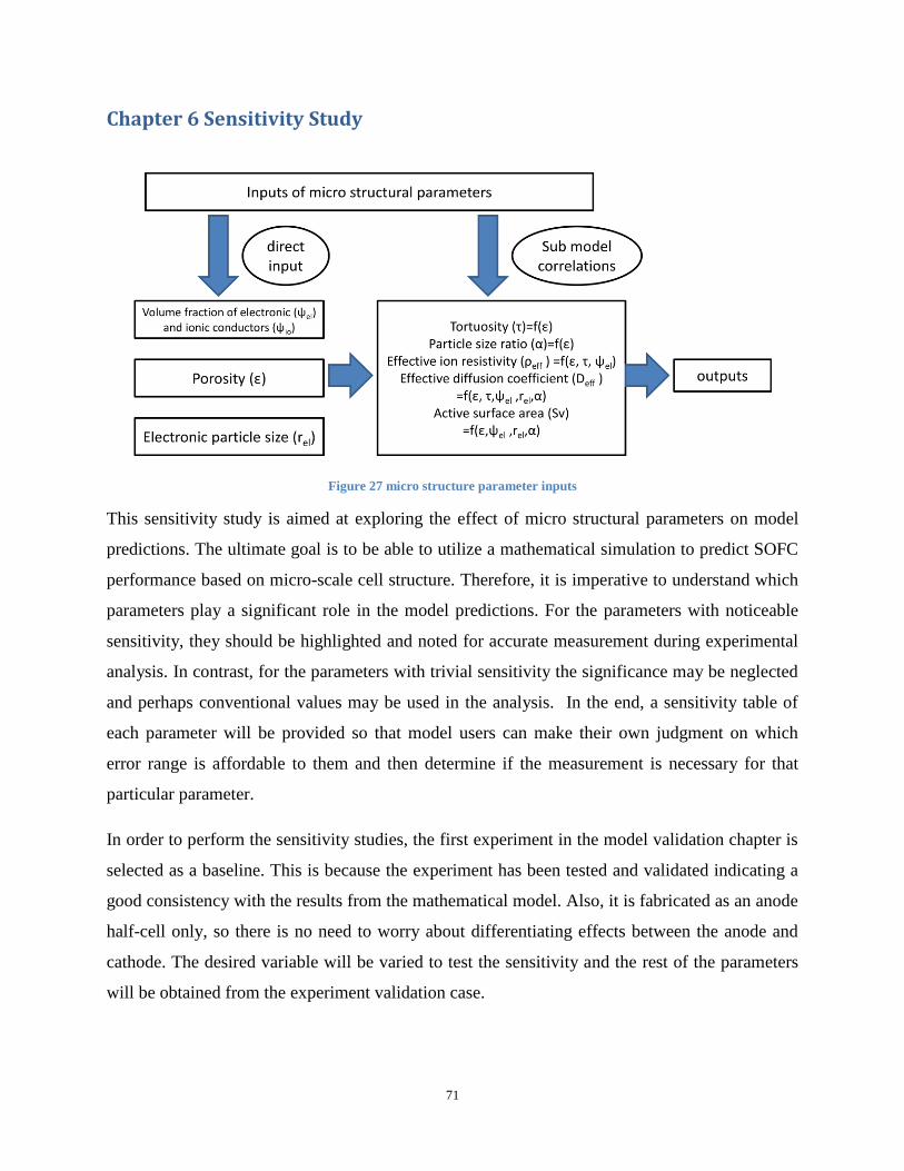
71
Chapter 6 Sensitivity Study
Figure 27 micro structure parameter inputs
This sensitivity study is aimed at exploring the effect of micro structural parameters on model
predictions. The ultimate goal is to be able to utilize a mathematical simulation to predict SOFC
performance based on micro-scale cell structure. Therefore, it is imperative to understand which
parameters play a significant role in the model predictions. For the parameters with noticeable
sensitivity, they should be highlighted and noted for accurate measurement during experimental
analysis. In contrast, for the parameters with trivial sensitivity the significance may be neglected
and perhaps conventional values may be used in the analysis. In the end, a sensitivity table of
each parameter will be provided so that model users can make their own judgment on which
error range is affordable to them and then determine if the measurement is necessary for that
particular parameter.
In order to perform the sensitivity studies, the first experiment in the model validation chapter is
selected as a baseline. This is because the experiment has been tested and validated indicating a
good consistency with the results from the mathematical model. Also, it is fabricated as an anode
half-cell only, so there is no need to worry about differentiating effects between the anode and
cathode. The desired variable will be varied to test the sensitivity and the rest of the parameters
will be obtained from the experiment validation case.
72
6.1 Sub Model Correlations
6.1.1 Tortuosity vs. Porosity
There are two places containing the tortuosity parameter in the model. They are related to ohmic
resistance in electrode and mass diffusion. First of all, based on eqn. (3.5), it can be found that
increasing tortuosity will result in a growing of effective ionic resistivity and hence worsen the
performance of SOFCs. Physically, if tortuosity increases, the transportation rate of ionic
conductors will be reduced due to a relatively long and twisting path from one end of the
electrode to the other end. Therefore, the effective ion resistivity is expected to increase. Since
electronic conductivity is several orders of magnitude higher than the ionic conductivity, ohmic
overpotential is primarily dominated by the resistance due to ionic conductors. That is why we
are mainly interested in effective ionic resistivity. Secondly, the parameter of tortuosity also
appears in the effective diffusivity to impact the gas diffusion process. From the eqn. (3.19), it
can be seen that the increase of tortuosity will result in a decrease in effective diffusion
coefficient. In that case, a larger tortuosity will lead to a lower concentration of fuel at electrode-
electrolyte interface and hence increase the concentration overpotential. This is represented in
the mathematical model as well. The concentration gradient will drop fast due to a large
tortuosity in eqn. (3.31) and thus increase the concentration overpotential due to eqn. (1.6).
For this particular case, the porosity is given as 30%. The idea is to vary the unknown parameter
n from eqn. (4.59) in order to find out how tortuosity impacts the model. Table 11, Table 12, and
Fig. 28 show comparison among different tortuosity values. The n-value is chosen to vary from
0.01 to 1 for 79%/21% Ni/YSZ, and from 0.01 to 1.3 for 83%/17% Ni/YSZ, respectively.
Tortuosity can be calculated by using eqn. (4.59). After that, each tortuosity value is applied into
the model to calculate the overall overpotential. The last column in Table 11 and Table 12 is to
compare the overpotential value calculated from the corresponding n values with experimental
data for two different volume fractions of Ni and YSZ. In this case, the experiment data is
represented by the mathematical model with n-value equal to 0.5. The purpose is to explore how
the n-value affects the overall overpotential. As shown in Table 11 and Table 12, the range of n-
value is proper selected so that the overall percentage difference is within around ±15%. After
the range is determined, the domain will be averagely divided into 20 sections plus one
additional point, the n-value equals to 0.5. And the same strategy will be applied for selecting the
ranges and points for the rest of the testing variables. In addition, Fig. 28 converts the table into

73
an x-y plot, the dashed region indicates the range of ±5% difference of overpotential by
compared with the experimental data. In order to maintain the change to be within 5% of the
error bars, the range of n-value is approximately from 0.275 to 0.685 for 79%/21% Ni/YSZ, and
from 0.08 to 0.79 for 83%/17% Ni/YSZ, respectively. Correspondingly, the tortuosity value and
percentage range is about 1.4 - 2.25 (-23.3% - 33.7%) for 79%/21% Ni/YSZ, and 1.1 - 2.5 (-39.6%
- 36.9%) for 83%/17% Ni/YSZ. It can be seen that the tortuosity value can vary over a relatively
large range (~ +/-40%) while having a small impact on the predicted overpotential (+/- 5%). This
indicates that the sensitivity of this factor is not that significant.

74
Table 11 comparison among different tortuosity for 79%/21% Ni/YSZ
n-value tortuosity ∑
0.010 1.012 -10.037%
0.062 1.078 -9.186%
0.114 1.147 -8.290%
0.166 1.222 -7.345%
0.218 1.301 -6.350%
0.271 1.385 -5.302%
0.323 1.475 -4.200%
0.375 1.570 -3.039%
0.427 1.672 -1.819%
0.479 1.780 -0.536%
0.500 1.826 0.000%
0.531 1.895 0.811%
0.583 2.018 2.226%
0.635 2.149 3.711%
0.687 2.288 5.268%
0.739 2.436 6.901%
0.792 2.594 8.612%
0.844 2.761 10.403%
0.896 2.940 12.278%
0.948 3.131 14.239%
1.000 3.333 16.288%
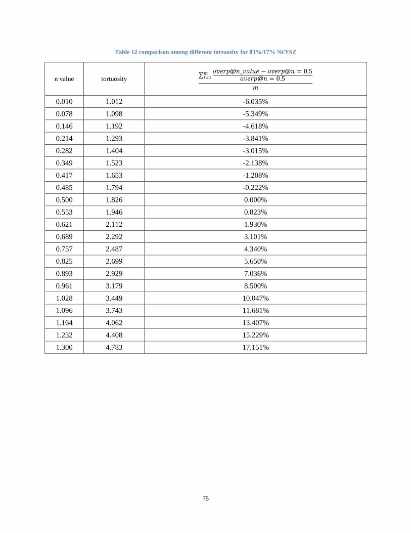
75
Table 12 comparison among different tortuosity for 83%/17% Ni/YSZ
n value tortuosity ∑
0.010 1.012 -6.035%
0.078 1.098 -5.349%
0.146 1.192 -4.618%
0.214 1.293 -3.841%
0.282 1.404 -3.015%
0.349 1.523 -2.138%
0.417 1.653 -1.208%
0.485 1.794 -0.222%
0.500 1.826 0.000%
0.553 1.946 0.823%
0.621 2.112 1.930%
0.689 2.292 3.101%
0.757 2.487 4.340%
0.825 2.699 5.650%
0.893 2.929 7.036%
0.961 3.179 8.500%
1.028 3.449 10.047%
1.096 3.743 11.681%
1.164 4.062 13.407%
1.232 4.408 15.229%
1.300 4.783 17.151%

76
(a) 79%/21% Ni/YSZ
(b) 83%/17% Ni/YSZ
Figure 28 comparison of anode overpotential at different n-value
6.1.2 Particle size ratio vs. porosity
From the mass transfer governing equation and active surface area formula, it can be found that
both mass diffusion and electrochemical reaction depend on the particle size ratio. Let us take
79%/21% Ni/YSZ as an example, the ion and electron particle size ratio need to be within 0.13
to 0.53 determined by coordination number model in order to maintain the threshold. Table 13
shows the proper range of particle size ratio. It can be found that as particle size ratio increases,
the active surface area decreases and results in a growth of overpotential. It is because as particle
size ratio gets smaller, the size difference of two types of conductors is expected to be more
significant. Therefore, there will be more of the smaller particles falling in the porous space
among large particles to increase the reaction sites at TPB region and hence improve the cell
performance. The particle size ratio impact of gas diffusion is not significant due to a relative
thin anode thickness. For both of the two volume fractions, the particle size ratio is strongly
sensitive. As shown in Figure 29 if the overpotential difference is expected to be within 5%
(dashed line region), the range of particle size ratio and its percentage needs to be 0.386 - 0.414
(-3.5% - 3.5%) for 79%/21% Ni/YSZ, and 0.376 - 0.385 (-1.3% - 1.1%) for 83%/17% Ni/YSZ.

77
Table 13 comparison among different particle size ratio for 79%/21% Ni/YSZ
Particle size ratio α Active surface area ∑
0.350 3.03E+05 -16.946%
0.355 2.96E+05 -15.544%
0.359 2.89E+05 -14.106%
0.364 2.82E+05 -12.631%
0.369 2.75E+05 -11.116%
0.374 2.68E+05 -9.559%
0.378 2.61E+05 -7.957%
0.383 2.55E+05 -6.307%
0.388 2.48E+05 -4.606%
0.393 2.42E+05 -2.850%
0.397 2.35E+05 -1.035%
0.400 2.32E+05 0.000%
0.402 2.29E+05 0.843%
0.407 2.23E+05 2.789%
0.412 2.17E+05 4.809%
0.416 2.11E+05 6.910%
0.421 2.05E+05 9.099%
0.426 1.99E+05 11.383%
0.431 1.93E+05 13.774%
0.435 1.87E+05 16.282%
0.440 1.81E+05 18.919%
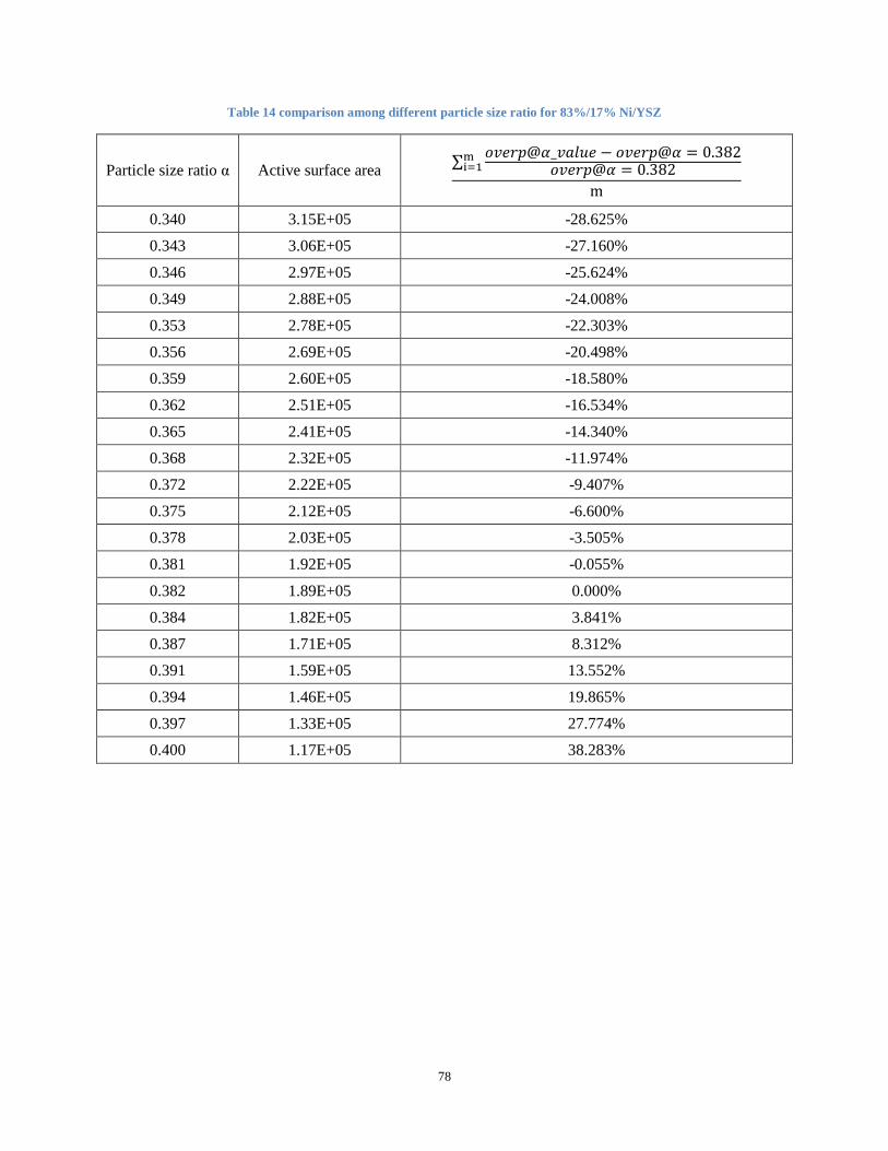
78
Table 14 comparison among different particle size ratio for 83%/17% Ni/YSZ
Particle size ratio α Active surface area ∑
0.340 3.15E+05 -28.625%
0.343 3.06E+05 -27.160%
0.346 2.97E+05 -25.624%
0.349 2.88E+05 -24.008%
0.353 2.78E+05 -22.303%
0.356 2.69E+05 -20.498%
0.359 2.60E+05 -18.580%
0.362 2.51E+05 -16.534%
0.365 2.41E+05 -14.340%
0.368 2.32E+05 -11.974%
0.372 2.22E+05 -9.407%
0.375 2.12E+05 -6.600%
0.378 2.03E+05 -3.505%
0.381 1.92E+05 -0.055%
0.382 1.89E+05 0.000%
0.384 1.82E+05 3.841%
0.387 1.71E+05 8.312%
0.391 1.59E+05 13.552%
0.394 1.46E+05 19.865%
0.397 1.33E+05 27.774%
0.400 1.17E+05 38.283%
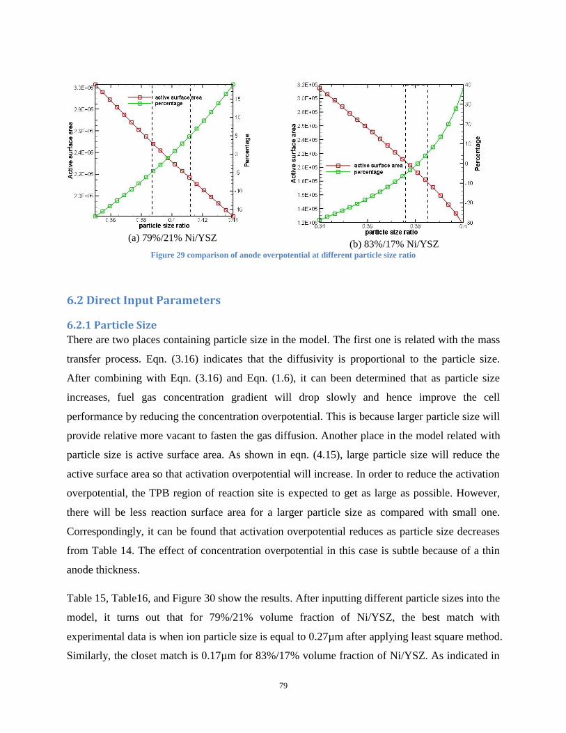
79
(a) 79%/21% Ni/YSZ
(b) 83%/17% Ni/YSZ Figure 29 comparison of anode overpotential at different particle size ratio
6.2 Direct Input Parameters
6.2.1 Particle Size
There are two places containing particle size in the model. The first one is related with the mass
transfer process. Eqn. (3.16) indicates that the diffusivity is proportional to the particle size.
After combining with Eqn. (3.16) and Eqn. (1.6), it can been determined that as particle size
increases, fuel gas concentration gradient will drop slowly and hence improve the cell
performance by reducing the concentration overpotential. This is because larger particle size will
provide relative more vacant to fasten the gas diffusion. Another place in the model related with
particle size is active surface area. As shown in eqn. (4.15), large particle size will reduce the
active surface area so that activation overpotential will increase. In order to reduce the activation
overpotential, the TPB region of reaction site is expected to get as large as possible. However,
there will be less reaction surface area for a larger particle size as compared with small one.
Correspondingly, it can be found that activation overpotential reduces as particle size decreases
from Table 14. The effect of concentration overpotential in this case is subtle because of a thin
anode thickness.
Table 15, Table16, and Figure 30 show the results. After inputting different particle sizes into the
model, it turns out that for 79%/21% volume fraction of Ni/YSZ, the best match with
experimental data is when ion particle size is equal to 0.27µm after applying least square method.
Similarly, the closet match is 0.17µm for 83%/17% volume fraction of Ni/YSZ. As indicated in

80
Figure 30, if the overpotential difference is considered to be within ±5% (as indicated within the
dashed line), the change of range of particle size is within 0.02µm, which is from –7.4% to 7.4%
in terms of percentage for 79%/21% volume fraction of Ni/YSZ. On the other hand, the ion
particle size needs to be between from to 0.156µm to 0.183µm (or -8.2% - 7.6%) for 83%/17%
volume fraction of Ni/YSZ. This factor has a strong sensitivity in the model. Thus this parameter
is extremely important in the model input and precise measurement is required. Also, the ion
particle range provided by the paper, which varies from 0.1-0.3μm, is not good enough for a
mathematical model to predict a solution within +/- 5%.
Table 15 comparisons of particle sizes for two different composition of 79%/21% Ni/YSZ
Ionic particle size (μm) ∑
0.210 -15.958%
0.215 -14.670%
0.219 -13.388%
0.224 -12.110%
0.229 -10.837%
0.234 -9.569%
0.238 -8.306%
0.243 -7.047%
0.248 -5.793%
0.253 -4.543%
0.257 -3.298%
0.262 -2.058%
0.267 -0.822%
0.270 0.000%
0.272 0.410%
0.276 1.637%
0.281 2.860%
0.286 4.078%
0.291 5.292%
0.295 6.502%
0.300 7.707%
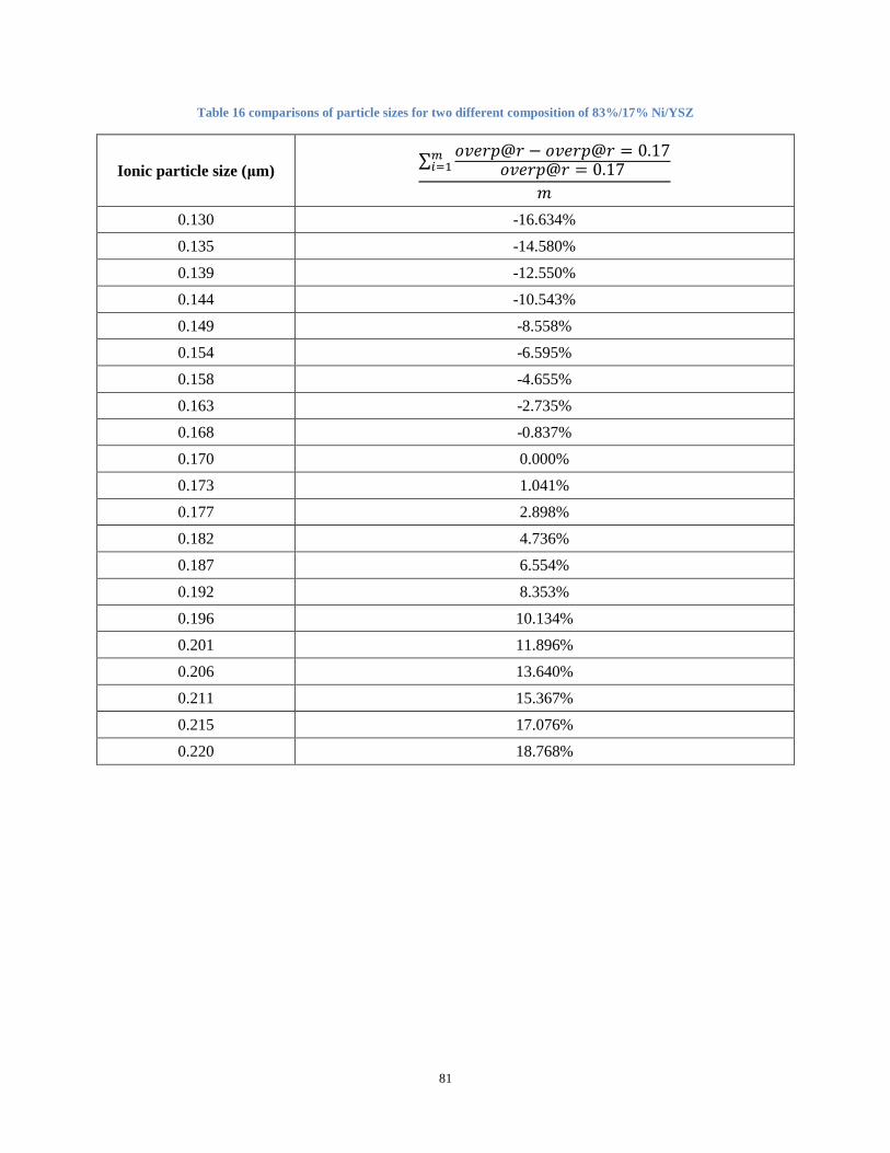
81
Table 16 comparisons of particle sizes for two different composition of 83%/17% Ni/YSZ
Ionic particle size (μm) ∑
0.130 -16.634%
0.135 -14.580%
0.139 -12.550%
0.144 -10.543%
0.149 -8.558%
0.154 -6.595%
0.158 -4.655%
0.163 -2.735%
0.168 -0.837%
0.170 0.000%
0.173 1.041%
0.177 2.898%
0.182 4.736%
0.187 6.554%
0.192 8.353%
0.196 10.134%
0.201 11.896%
0.206 13.640%
0.211 15.367%
0.215 17.076%
0.220 18.768%

82
(a) 79%/21% Ni/YSZ
(b) 83%/17% Ni/YSZ
Figure 30 comparisons of particle sizes for two different composition of Ni/YSZ
6.2.2 Porosity
All three different overpotentials are a function of porosity. Eqn. (3.5) indicates that the ohmic
resistance within the electrodes will increase as porosity increases. On the other hand, it can be
concluded from eqn. (3.15) that a larger porosity will make the effective diffusivity increase.
Thus, fuel gas concentration gradient will drop slowly as indicated from eqn. (3.31) and result in
a relatively larger concentration at TPB region. This will cause the concentration overpotential to
reduce. Physically, increasing the porosity will reduce the solid parts in the electrodes, which is
unfavorable for ion transport through particles. However, it will facilitate gas diffusion as more
channels are available in a larger porous structure. Furthermore, eqn. (4.15) shows that active
surface area will decrease with the increase of porosity. Therefore, a relative small porosity can
enhance the electrochemical reaction by providing more reaction area and reduce the activation
overpotential.
The porosity of 79%/21% Ni/YSZ is listed in Table 17 and Table 18 shows the comparison of
porosity for 83%/17% Ni/YSZ. The selected porosity range has to maintain the threshold of
same particles throughout the electrode connected with each other to form a good conductivity
pathway. Therefore, for different compositions of Ni and YSZ, the porosity range need to be
calculated by combining the coordination number model and porosity and particle size ratio sub
model. It can be seen that the overpotential difference increases as porosity increases. This is
because the activation overpotential is dominant as compared with ohmic and concentration

83
overpotential due to a thin anode thickness. The test results are consistent with the
aforementioned physical analysis.
Table 17 comparison of porosity for 79%/21% Ni/YSZ
Porosity (%) ∑
0.270 -17.651%
0.273 -15.926%
0.276 -14.175%
0.279 -12.394%
0.283 -10.584%
0.286 -8.742%
0.289 -6.866%
0.292 -4.953%
0.295 -3.003%
0.298 -1.012%
0.300 0.000%
0.302 1.023%
0.305 3.103%
0.308 5.233%
0.311 7.414%
0.314 9.652%
0.317 11.949%
0.321 14.309%
0.324 16.738%
0.327 19.241%
0.330 21.822%

84
Table 18 comparison of porosity for 83%/17% Ni/YSZ
Porosity (%) ∑
0.280 -21.617%
0.282 -20.293%
0.283 -18.922%
0.285 -17.501%
0.286 -16.026%
0.288 -14.491%
0.289 -12.892%
0.291 -11.222%
0.293 -9.474%
0.294 -7.640%
0.296 -5.710%
0.297 -3.672%
0.299 -1.514%
0.300 0.000%
0.301 0.781%
0.302 3.233%
0.304 5.864%
0.305 8.704%
0.307 11.790%
0.308 15.171%
0.310 18.908%
As shown in Figure 31, if a ±5% difference of overpotential needs to be satisfied (as indicated
within the dashed line region), the porosity range is from 0.291 to 0.306 (or -3.0% - 2.0%) for
79%/21% Ni/YSZ, and from 0.296 to 0.303 (or -1.3% - 1.0%) for 83%/17% Ni/YSZ respectively.
This indicates that this quantity is highly sensitive. Therefore, an accurate measurement may be
needed to perform accurate predictions from the model.

85
(a) 79%/21% Ni/YSZ
(b) 83%/17% Ni/YSZ
Figure 31 comparisons of porosity for two different composition of Ni/YSZ
6.2.3 Volume Fraction
First of all, volume fraction affects the ohmic overpotential. As indicated from eqn. (3.5), as ion
volume fraction increases, ohmic overpotential deceases. Next, active surface area is a function
of volume fraction as well. However, this quantity in active surface area formula is highly
nonlinear and hence it is too complex to analyze the detailed influence. As shown in Fig. 32, if
the overpotential difference is restricted to ±5%, the adjustable range of electron volume fraction
is from 0.781 to 0.797 (or -1.1% - 0.8%) for 79%/21% volume fraction Ni/YSZ, and from 0.8275
to 0.832 (or -0.3% - 0.2%) for 83%/17% volume fraction Ni/YSZ respectively. Therefore,
volume fraction value is extremely crucial for predicting SOFC performance.
86
Table 19 comparison of volume fraction for 79%/21% Ni/YSZ
Electronic conductor
volume fraction (%) ∑
74.000 -18.521%
74.368 -17.701%
74.737 -16.819%
75.105 -15.873%
75.474 -14.856%
75.842 -13.763%
76.211 -12.588%
76.579 -11.324%
76.947 -9.962%
77.316 -8.491%
77.684 -6.901%
78.053 -5.177%
78.421 -3.302%
78.789 -1.256%
79.158 0.000%
79.526 0.987%
79.895 3.458%
80.263 6.196%
80.632 9.253%
81.000 12.698%
74.000 16.622%

87
Table 20 comparison of volume fraction for 83%/17% Ni/YSZ
Electronic conductor
volume fraction (%) ∑
82.000 -16.303%
82.079 -15.381%
82.158 -14.415%
82.237 -13.403%
82.316 -12.340%
82.395 -11.221%
82.474 -10.041%
82.553 -8.793%
82.632 -7.470%
82.711 -6.063%
82.789 -4.562%
82.868 -2.955%
82.947 -1.227%
83.000 0.000%
83.026 0.639%
83.105 2.665%
83.184 4.877%
83.263 7.311%
83.342 10.009%
83.421 13.030%
83.500 16.451%

88
(a) 79%/21% Ni/YSZ
(b) 83%/17% Ni/YSZ
Figure 32 comparisons of volume fraction of Ni/YSZ
6.3 Summary To sum up, Table 21 lists the results of sensitivity study for the microstructure parameters in the
numerical model at two different volume fractions. It can be seen that the model is extremely
sensitive to volume fraction, porosity and particle size ratio. These parameters can only be varied
within a narrow range, which is within ±3.5% for all three in order to maintain a ±5% change in
the predicted overpotential for both of the volume fractions. Furthermore, among those
parameters, volume fraction is the most sensitive one. If the measurement has ±1% error, the
error of the results will be ±5%. Therefore, a careful measurement is highly suggested for
particle size ratio, porosity, and volume fraction. Next, as the variation of overpotential is within
±5%, the particle size changes at around ±8%. It is also a sensitive factor, but not as much as
particle size ratio. As mentioned before, particle size ratio is strongly sensitive and needs to be
measured. Since the only way to measure particle size ratio is to measure particle size, particle
size also needs to be counted as a significant sensitive quantity and require careful measurement.
However, the model does not seem to be very sensitive to tortuosity. For a small percent change
of overpotential, ±5%, the model can allow the tortuosity to vary up to ±20% to ±30%. Besides,
this factor is the most difficult parameter to perform a measurement of in an experiment.
Therefore, the porosity-tortuosity correlation we adapt may be valid to approximate tortuosity
depending on the accuracy requirement.

89
Table 21 Results of parameter sensitivity study
Percent change corresponding to +/- 5% change in predicted overpotential
Parameter 79%Ni / 21% YSZ 83% Ni / 17% YSZ
Tortuosity -23.3% - 33.7% -39.6% - 36.9%
Particle size ratio -3.5% - 3.5% -1.3% - 1.1%
Particle size -7.4% - 7.4% -8.2% - 7.6%
Porosity -3% - 2% -1.3% - 1.0%
Volume fraction -1.1% - 0.8% -0.3% - 0.2%

90
Chapter 7 Functionally Graded Electrodes
7.1 Boundary condition treatment
Another goal of our research is to implement and modify this model so that it can be applied in
more complicated scenarios, such as FGEs. To accomplish this, the boundary conditions of our
original model needed to be reconsidered. It required a more general treatment of boundary
conditions so that they could fit the multiple layers and micro structural grading of electrodes. In
the original model, the overall overpotential gradient at the EE interface is given as the product
of effective resistivity at fuel channel and total current density. This is fine for conventional
electrodes, since all the micro structural parameters are uniform throughout the electrode.
However, it is incorrect for FGEs because the effective resistivity varies with different types of
grading and the value at EE interface may not be the same as the one at fuel channel. In order to
solve this problem, what we did is use an iterative method to adjust the overpotential value after
each computing cycle until meet our requirement, which is to force electron current density equal
to zero. Several linear-interpolation approaches can accomplish this job such as the Secant
method (54).
7.2 Comparison between FGEs and non-FGEs SOFCs In order to test if FGEs will provide better performance for SOFCs, a SOFC with FGEs will be
studied and compared with conventional electrodes SOFC. Again, let us select the microstructure
parameters from Jiang’s experimental data to do the analysis.
Table 22 list of microstructure parameters change with porosity
Porosity (%) Particle size ratio (rio/rel) Active surface area (m2/m
3)
20 0.202 6.65105
30 0.396 2.19105
40 0.513 0.64105
The above table lists how the particle size ratio and active surface area changes with porosity. By
applying porosity and particle size ratio correlation, it can be found out that as porosity gets
bigger, particle size ratio also appears to be larger. Larger particle size ratio means the size
difference between two types of conductors is becoming smaller. In addition, according to
coordination number model, active surface area starts to drop with increasing of porosity.
Physically, relative large porosity will be favorable for diffusion process because it will generate
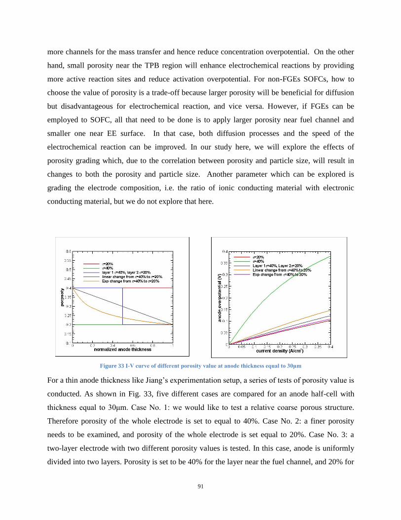
91
more channels for the mass transfer and hence reduce concentration overpotential. On the other
hand, small porosity near the TPB region will enhance electrochemical reactions by providing
more active reaction sites and reduce activation overpotential. For non-FGEs SOFCs, how to
choose the value of porosity is a trade-off because larger porosity will be beneficial for diffusion
but disadvantageous for electrochemical reaction, and vice versa. However, if FGEs can be
employed to SOFC, all that need to be done is to apply larger porosity near fuel channel and
smaller one near EE surface. In that case, both diffusion processes and the speed of the
electrochemical reaction can be improved. In our study here, we will explore the effects of
porosity grading which, due to the correlation between porosity and particle size, will result in
changes to both the porosity and particle size. Another parameter which can be explored is
grading the electrode composition, i.e. the ratio of ionic conducting material with electronic
conducting material, but we do not explore that here.
Figure 33 I-V curve of different porosity value at anode thickness equal to 30μm
For a thin anode thickness like Jiang’s experimentation setup, a series of tests of porosity value is
conducted. As shown in Fig. 33, five different cases are compared for an anode half-cell with
thickness equal to 30μm. Case No. 1: we would like to test a relative coarse porous structure.
Therefore porosity of the whole electrode is set to equal to 40%. Case No. 2: a finer porosity
needs to be examined, and porosity of the whole electrode is set equal to 20%. Case No. 3: a
two-layer electrode with two different porosity values is tested. In this case, anode is uniformly
divided into two layers. Porosity is set to be 40% for the layer near the fuel channel, and 20% for

92
the other layer. Case No. 4: a linear change of porosity within the whole electrode will be
considered. Thus, we would like to vary porosity starting from 40% in the fuel channel to 20% at
EE interface. Case No. 5: Other than linearity, it is necessary to test a different curvature shape
of porosity variation in the electrode such as exponential change. This time the porosity changes
exponentially from 40% at fuel channel to 20% at EE surface. Due to the shape of an exponential
function, most of the porosity value will be close to 20%. The plots of Fig. 33 indicate that
overpotential depends on porosity mainly, and smaller porosity will result in better performance.
This result is reasonable and can be interpreted from a detailed analysis in Fig. 34.
(a) distribution of current density
in electron conductor
(b) distribution of anode
overpotential
(c) distribution of H2 molar
concentration
Figure 34 detailed plots of anode thickness=30μm and current density=0.4A/cm2
Fig. 34 (c) shows the distribution of H2 in the normalized anode. Since the anode thickness is
extremely thin, there is almost no diffusion resistance in the whole electrode and that makes
concentration of H2 at EE surface remain almost the same as inlet condition. On other hand, it
can be seen from Fig. 34 (a) that electrochemical reaction occurs throughout the whole anode
and that makes activation overpotential dominate the whole overpotential. Since smaller porosity
will provide larger active surface area and hence reduce activation overpotential, it can be found
out from Fig. 34 (b) that, the electrode with 20% porosity has the minimum overpotential, while
40% has the maximum overpotential. Exponential change of porosity has the second minimum
overpotential, and it is due to most of the porosity value is close to 20%. In this case,
electrochemical reaction will be fastened at small porosity region. As a result, the two-layer
electrode turns out showing better performance compared with a linear change porosity electrode.
In the previous tests, diffusion does not play an important role due to an extremely thin anode
thickness. Next, we would like to take this factor into consideration and explore how the FGEs
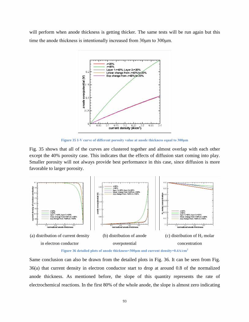
93
will perform when anode thickness is getting thicker. The same tests will be run again but this
time the anode thickness is intentionally increased from 30μm to 300μm.
Figure 35 I-V curve of different porosity value at anode thickness equal to 300μm
Fig. 35 shows that all of the curves are clustered together and almost overlap with each other
except the 40% porosity case. This indicates that the effects of diffusion start coming into play.
Smaller porosity will not always provide best performance in this case, since diffusion is more
favorable to larger porosity.
(a) distribution of current density
in electron conductor
(b) distribution of anode
overpotential
(c) distribution of H2 molar
concentration
Figure 36 detailed plots of anode thickness=300μm and current density=0.4A/cm2
Same conclusion can also be drawn from the detailed plots in Fig. 36. It can be seen from Fig.
36(a) that current density in electron conductor start to drop at around 0.8 of the normalized
anode thickness. As mentioned before, the slope of this quantity represents the rate of
electrochemical reactions. In the first 80% of the whole anode, the slope is almost zero indicating

94
that there is no electrochemical reaction occurs. After that, the slope drops significantly and
electrochemical reaction starts to take place. Fig. 36(b) also proves that diffusion process is more
dominant up to 80% of the whole anode and then takes over by electrochemical reactions.
Moreover, compared with Fig. 34(c), the drop of H2 molar concentration at EE interface is
significant in Fig. 36(c). This is shows that diffusion process is expected to have more of an
effect as thickness of electrode increases.
In the end, a typical anode-supported cell is tested as well. This time anode thickness is chosen to
be equal to 1000μm. As shown in Fig. 37, the linear change porosity and two-layer porosity
anode have lower overpotential than the uniform 20% and exponential distribution of porosity.
Figure 37 I-V curve of different porosity value at anode thickness equal to 1000μm
The results are anticipated and reasonable as it is consistent with the physics. Concentration
overpotential due to diffusion process becomes more important as anode thickness gets thicker.
Fig. 38 (a) shows that electrochemical reaction only takes place within about 10% of the whole
anode near EE interface, elsewhere is dominated by mass transfer. Larger porosity will benefit
diffusion and thus can reduce concentration overpotential. As indicated in Fig. 38 (c), the
electrode with 40% porosity has the minimum concentration overpotential, since this porosity
value will facilitate mass transfer and make molar concentration H2 to be highest at EE interface.
Same conclusion can also be found in Fig. 38 (b), which is the overpotential distribution in the

95
normalized anode. For almost 90% of anode starting from fuel channel, overall overpotential is
governed by concentration overpotential and anode with 40% porosity has the minimum overall
overpotential. As it approaches the EE surface, activation overpotential starts to climb
dramatically. Anodes with smaller porosity have a higher slope representing a faster reaction rate.
(a) distribution of current density
in electron conductor
(b) distribution of anode
overpotential
(c) distribution of H2 molar
concentration
Figure 38 detailed plots of anode thickness=1000μm and current density=0.4A/cm2
From the above analysis, we can see that almost 90% of the anode is governed by mass transfer
and the rest is dominated by electromechanical reactions. In order to further improve the cell
performance, a two-layer porosity grading is proposed. In the first 90% of anode thickness, a
larger porosity, 40%, will be applied to boost mass transfer process. On the other hand, for the
rest of anode, a smaller porosity, 20%, is used to enhance electrochemical reactions. The black
curve in Fig. 39 does show a best performance compared with the previous tests demonstrating a
consistency of physical assumption and mathematical simulation.
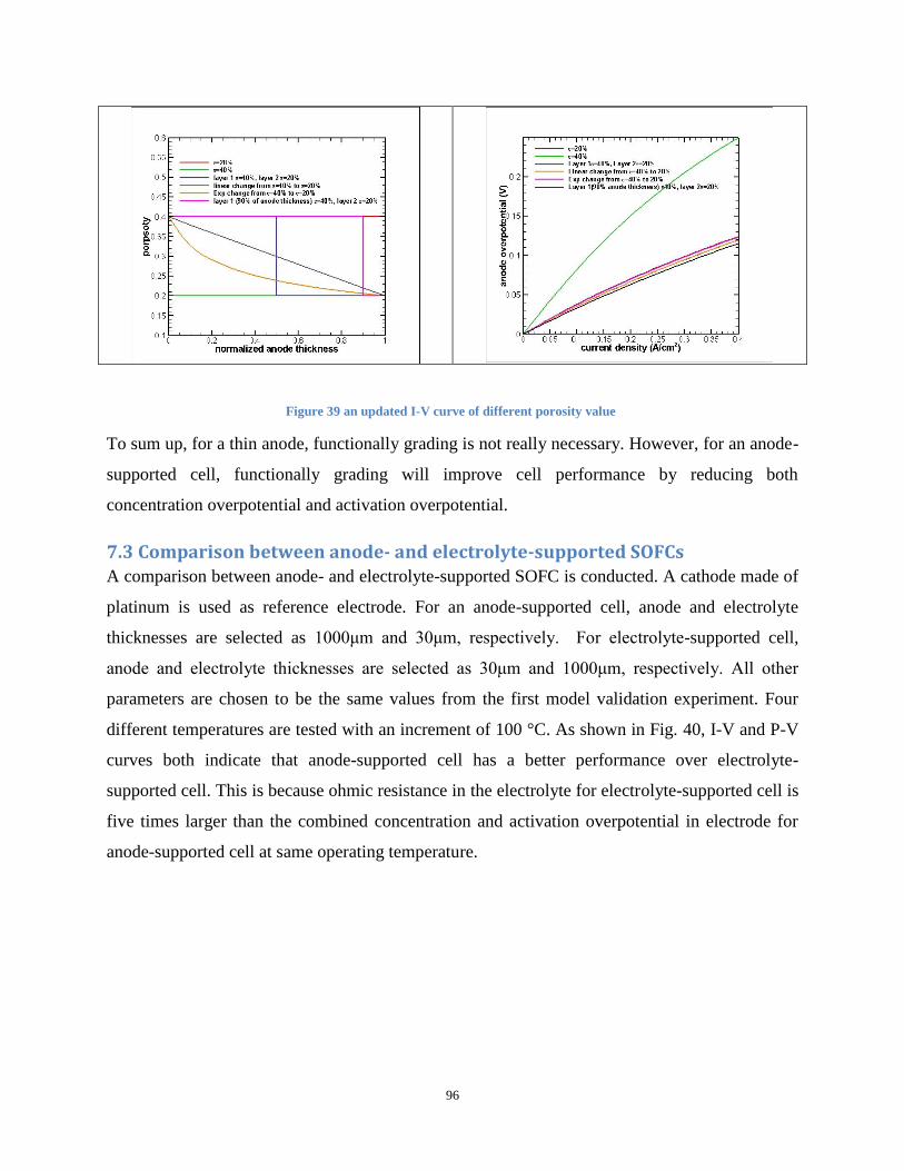
96
Figure 39 an updated I-V curve of different porosity value
To sum up, for a thin anode, functionally grading is not really necessary. However, for an anode-
supported cell, functionally grading will improve cell performance by reducing both
concentration overpotential and activation overpotential.
7.3 Comparison between anode- and electrolyte-supported SOFCs A comparison between anode- and electrolyte-supported SOFC is conducted. A cathode made of
platinum is used as reference electrode. For an anode-supported cell, anode and electrolyte
thicknesses are selected as 1000μm and 30μm, respectively. For electrolyte-supported cell,
anode and electrolyte thicknesses are selected as 30μm and 1000μm, respectively. All other
parameters are chosen to be the same values from the first model validation experiment. Four
different temperatures are tested with an increment of 100 °C. As shown in Fig. 40, I-V and P-V
curves both indicate that anode-supported cell has a better performance over electrolyte-
supported cell. This is because ohmic resistance in the electrolyte for electrolyte-supported cell is
five times larger than the combined concentration and activation overpotential in electrode for
anode-supported cell at same operating temperature.
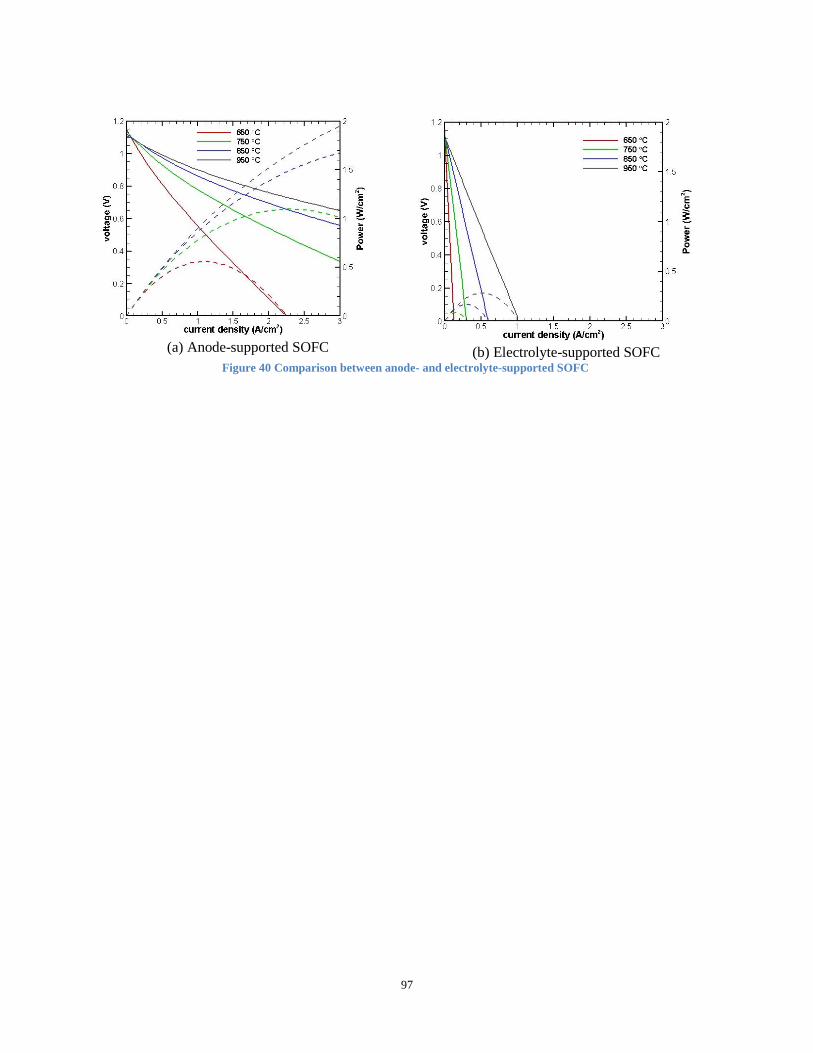
97
(a) Anode-supported SOFC
(b) Electrolyte-supported SOFC
Figure 40 Comparison between anode- and electrolyte-supported SOFC
98
Chapter 8 Conclusions In this study, SOFC performance has been investigated by a comprehensive mathematical model
that can simulate both mass transfer and electrochemical reactions for both electrodes from a
micro-scale level. The relationship of microstructure parameters such as the particle size of two
types of conductors, tortuosity and porosity were explored. Two sub model correlations, i.e.,
porosity and tortuosity, particle size ratio and porosity are adopted and implemented in the model
in order to mimic the SOFCs more closely to the practical situation. Next, three experiments that
aimed to examine SOFCs from different perspectives selected from literature to perform the
model validation. The numerical predictions agreed reasonably well with the experimental data
indicating a strong reliability of mathematical model and proper selection of sub model
correlations. After that, a sensitivity study of microstructure parameters and adopted sub model
correlations were tested. We achieved the goal to provide a benchmark so that scientists can
determine the precision of measurements required make reasonably accurate performance
predictions from the model. Moreover, we illustrated that FGEs can be applied to SOFCs in
order to achieve better cell efficiency when compared with uniform electrodes.

99
Works Cited 1. http://www.doitpoms.ac.uk/tlplib/fuel-cells/printall.php. univerisity of cambridge. [Online]
2. http://ogniwa-paliwowe.info/sofc.php. [Online]
3. Jeffrey W. Fergus, Rob Hui, Xianguo Li, David P. Wilkinson, Jiujun Zhang. Solid Oxide
FUel Cells materials Properties and Performance. Boca Raton : CRC Press, 2009.
4. Zirconia-based solid electrolytes: microstructure, stability and ionic conductivity. Badwal, S.
P.S. 1-3, 1992, Solid State Ionics, Vol. 52, pp. 23-32.
5. A review on the status of anode materials for solid oxide fuel cells. W.Z. Zhu, S.C. Deevi. 20
03, Materials Science anf Engineering, Vol. A362, pp. 228-239.
6. Ionic Conductivity of Nanocrystalline Yttria-Stablized Zirconia: Grain Boundry and Size Effec
ts. Dura, O.J., et al., et al. 2010, Chemical Reviews, p. 81.
7. Oxidation-Reduction Behavior of Undoped and Sr-Doped LaMnO3: Defect Structure, Electric
al Conductivity, and Thermoelectric Power. J.H. Kuo, H.U. Anderson. 1, 1990, Solid State Che
mistry, Vol. 87, pp. 55-63.
8. Thermodynamic analysis on interface between perovskite electrode and YSZ electrolyte. Yoko
kawa H, Sakai N, Kawada T, Dokiya M. 1990, Solid State Ionics, Vols. 40-41, pp. 398-401.
9. Ryan O'Hayre, Suk-Won Cha, Whitney Colella, Fritz B. Prinz. Fuel Cell Fundamentals (2
nd ed.). s.l. : John Wiley & Sons, Inc., Hoboken, New Jersey, 2009.
10. Micro-Scale Modleing of a Funcationally Graded Ni-YSZ Anode. M. Ni, M.K.H. Leung, D.
Y.C. Leung. 5, 2007, Chem. Eng. Technol. , Vol. 30, pp. 587-592.
11. Tortuosity in anode-supported proton conductive solid oxide fuel cell found from current flo
w rates and dusty-gas model. Chih-Long Tsai, V. Hugo Schmidt. 2011, journal of Power Sourc
es, Vol. 196, pp. 692-699.
12. fabrication and performance of Ni/3 mol% Y2O3-ZrO2 cermet andoes for solid oxide fuel cel
ls. S.P. Jiang, p.J. Callus, S.P.S Badwal. 132, 2000, Solid State Ionics, pp. 1-14.
13. Nanostructured and functionally graded cathodes for intermediate temperature solid oxide fu
el cells. Ying Liu, Charles Compson, Meilin Liu. 1-2, 2004, Journal of Power Sources, Vol. 13
8, pp. 194-198.
14. Modeling Elementary Heterogeneous Chemistry and Electrochemistry in Solid-Oxide Fuel C
ells. Huayang Zhu, Robert J. Kee, Vinod M. Janardhanan, Olaf Deutschmann, David G. G
oodwin. 152 (12) (2005), Journal of The Electrochemical Society, pp. A2427-A2440.

100
15. Lee, Won Yong. Modeling of Solid Oxide Fuel Cells. s.l. : MIT master thesis, 2006.
16. Performance comparison of Fick's, dusty-gas and Stefan_Maxwell models to predict the conc
entration overpotential of a SOFC anode. R. Suwanwarangkul, E. Croiset, M.W. Fowler, P.L.
Douglas, E. Entchev, M.A. Douglas. 122 (2003), Journal of Power Sources, pp. 9-18.
17. Anode Micro Model of Solid Oxide Fuel Cell. Xia, S.H. Chan Z.T. 148 (4) (2001), Journal o
f The Electrochemical Society, pp. A388-A394.
18. Mass transfer in graded microstructure solid oxide fuel cell electrodes. Eric S. Greene, Wils
on K.S. CHiu, Maria G. Medeiros. 161, 2006, Journal of Power Sources, pp. 225-231.
19. Micro-modelling of solid oxide fuel cell electordes. Paola Costamagna, Paolo Costa, Vince
zo Antonucci. 1998, Electrochimica Acta., Vol. 43, pp. 375-394.
20. Relation between percolation and particle corrdination in binary power mixtures. D. Bouvar
d, F.F. Lange,. 1991 : s.n., Acta Metall. Mater., Vol. 39, pp. 3080-3090.
21. Qnantification of SOFC anode microstructure based on dual beam FIB-SEM technique. Hiro
shi Iwai, et al. 2010, Journal of Power SOurces, Vol. 195, pp. 955-964.
22. Diffusion Limitations in the Porous Anodes of SOFCs. R.E. Williford, et al. 8, 2003, Journal
of the Electrochemical society, Vol. 150, pp. A1067-A1072.
23. Nondestructive Reconstruction and Analysis of SOFC Anodes Using X-ray computed tomogr
aphy at sub-50nm Resolution. John R. Izzo, et al. 5, 2008, Journal of the electrochemical societ
y, Vol. 155, pp. B504-B508.
24. Cussler, E.L. Diffusion: Mass transfer in fluid systems. cambridge : cambridge university pr
ess, 1995.
25. Fuel composition and diluent effect on gas transport and performance of anode supported S
OFCs. Yi Jiang, Anil V. Virkar. 7, 2003, Journal of the electrochemical society, Vol. 150, pp.
A942-A951.
26. Tortuosity-porosity relation in porous media flow. Maciej Matyka, Arzhang Khalili, and Z
bigniew Koza. 026306-1 ~026306-8, 2008, Phys. Rev. E , Vol. 78.
27. Archie, G. 1942, Metallurgical and Petroleum Engineers, Vol. 146, p. 54.
28. Effective Diffusion Coefficient in Porous Media. WEISSBERG, HAROLD L. 1963, Appl. P
hys., Vol. 34, pp. 2636-2639.
29. J. Comiti, M. Renaud. 1989, Chem. Eng. Sci., Vol. 44, p. 1539.

101
30. Tortuosity of Porous Particles. M. Barrande, R. Bouchet, R. Denoyel. 2007, Anal. Chem.,
Vol. 79, pp. 9115-9121.
31. Diffusion coefficients of sulfate and methane in marine sediments: Influence of porosity. N. I
VERSEN, B. B. Jorgensen. 1993, Geochimica et Cosmochimica Acta, Vol. 57, pp. 571-578.
32. Predicted tortuosity of muds. Bernard P. Boudreau, Filip J.R. Meysman. 2006, Geology,
Vol. 34, pp. 693-696.
33. German, Randall M. Particle packing characteristics. s.l. : Princeton, N.J. : Metal Powder I
ndustries Federation, 1989.
34. Impact of anode microstructure on solid oxide fuel cells. Toshio Suzuki, Zahir Hasan, Yos
hihiro Funahashi, Toshiaki Yamaguchi, Yoshinobu Fujishiro, Masanobu Awano. 2009, Sic
ence, Vol. 325, pp. 852-855.
35. Tortuosity variation in a low density binary particulate bed. Ricardo Dias, Jose A. Teixeira,
Manuel Mota, Alexander Yelshin. 2006, Separation and Purification Technology, Vol. 51, pp.
180-184.
36. Dense Random Packing of Binary Mixtures of Spheres. S. Yerazunis, S. W. Cornell and B.
Wintner. 1965, Nature, Vol. 207, pp. 835-837.
37. Functionally graded composite cathodes for solid oxide fuel cells. N.T. Hart, N.P. Brandon,
M.J. Day, N.Lapena-Rey. 2002, Journal of Power Source, Vol. 106, pp. 42-50.
38. Functionally graded cathodes fabricated by sol-gel/slurry coating for honeycomb SOFCs. Sh
aowu Zha, Yuelan Zhang, Meilin Liu. 2005, Solid State Ionics, Vol. 176, pp. 25-31.
39. Computational Analysis of Solid Oxide Fuel Cell with Functioanlly Graded Electrodes. Cha
o Wang, George Huang, Ryan Miller. Orlando : AIAA, 2011-272. AIAA.
40. Mathematical modeling of planar solid oxide fuel cells. M.M. Hussain, X. Li, I. Dincer. 161
(2006), Journal of Power Sources, pp. 1012–1022.
41. On Gaseous Self-Diffusion in Long Capillary Tubes. W.G. POLLARD, R. D. Present. 1948,
Physical Review, Vol. 73, pp. 762-774.
42. A macro-level model for determining the performance characteristics of solid oxide fuel cells.
Eduardo Hern andez-Pachecoa, Devinder Singh, Phillip N. Hutton, Nikhil Patel, Michael
D. Mann. 138 (2004), Journal of Power Sources, pp. 174-186.
43. comprehensive micro-scale model for transport and reaction in intermediate temperature sol
id oxide fuel cells. Jin Hyun Nam, Dong Hyup Jeon. 51 (2006), Electrochimica Acta , pp. 3446
–3460.

102
44. Berger, Carl. Handbook of Fuel Cell Technology. s.l. : Prentice-Hall Inc., Englewood Cliffs,
New Jersey, 1968.
45. Rigidity and conductivity percolation thresholds in particulate composites. C.H. Kuo, P.K.
Gupta. 1995, Acta Metall, Mater., Vol. 43, pp. 397-403.
46. Chemisorption of Hydrogen on the (111) Plane of Nickel. J. Lapujoulade, K. S. Neil. 8, 197
2, Journal of Chemical Physics, Vol. 57, p. 3535.
47. Relationship between the steady-state polarization of the SOFC air electrode, La0.6Sr0.4Mn
O3 /YSZ, and its complex impedance measured at the equilibrium potential. Yoshio Matsuzaki,
Isamu Yasuda. 3-4, 1999, Solid State Ionics, Vol. 126, pp. 307-313.
48. Serway, Raymond A. Principles of Physics (2nd ed.). Fort Worth, Texas : London: Saunder
s College Pub., 1998.
49. Electronic conductivity, Seebeck coefficient, defect and electronic structure of nonstoichiome
tric La1-xSrxMnO3. Junichiro Mizusakia et al. 2000, Solid State Ionics, Vol. 132, pp. 167-180.
50. J.A. Currie, Br. 1960, J. Appl. Phys., Vol. 11, pp. 318-324.
51. Performance and electrode behaiour of nano-YSZ impregnated nickel anodes used in solid o
xide fuel cells. S.P.Jiang, W. Wang, Y.D. Zhen. 2005 : s.n., Journal of Power Sources, Vol. 147,
pp. 1-7.
52. Performance and durability of Ni-coated SZ anodes for intermediate temperature solid oxide
fuel cells. Sun-Dong Kim, Hwan Moon, Sang-Hoon Hyun, Jooho Moon, Joosu Kim, Hae-W
eon Lee. 2006, Solid State Ionics, pp. 931-938.
53. http://en.wikipedia.org/wiki/Secant_method. [Online]
54. Micro-Scale Modelling of solid oxide fuel cells with micro-sturcurally graded electrodes. Me
ng Ni, Michael K. H. Leung, Dennis Y.C. Leung. 168 (2007), Journal of Power Sources, pp. 3
69-378.
55. Functionally graded cathodes for solid oxide fuel cells. Hart, N.T., et al., et al. 2001, Journa
l of materials science, pp. 1077-1085.