Emergent Power-Law Phase in the 2D Heisenberg Windmill Antiferromagnet:A Computational Experiment

Bhilahari Jeevanesan,1 Premala Chandra,2 Piers Coleman,2, 3 and Peter P. Orth1, 4

1Institute for Theory of Condensed Matter, Karlsruhe Institute of Technology (KIT), 76131 Karlsruhe, Germany2Center for Materials Theory, Rutgers University, Piscataway, New Jersey 08854, USA

3Hubbard Theory Consortium and Department of Physics,Royal Holloway, University of London, Egham, Surrey TW20 0EX, UK

4School of Physics and Astronomy, University of Minnesota, Minneapolis, Minnesota 55455, USA(Dated: June 15, 2015)

In an extensive computational experiment, we test Polyakov’s conjecture that under certain cir-cumstances an isotropic Heisenberg model can develop algebraic spin correlations. We demonstratethe emergence of a multi-spin U(1) order parameter in a Heisenberg antiferromagnet on interpene-trating honeycomb and triangular lattices. The correlations of this relative phase angle are observedto decay algebraically at intermediate temperatures in an extended critical phase. Using finite-sizescaling, we show that both phase transitions are of the Berezinskii-Kosterlitz-Thouless type and atlower temperatures, we find long-range Z6 order.

PACS numbers: 75.10.-b, 75.10.Jm

In statistical mechanics it is assumed [1, 2] that 2DHeisenberg magnets cannot develop algebraic order atfinite temperatures since interaction of the Goldstonemodes causes the spin-wave sti↵ness to renormalize tozero. However, in his pioneering work on this subject [3],Polyakov speculated that a 2D Heisenberg magnet mightdevelop algebraic order if the system were to developa “vacuum degeneracy”; he further suggested that thispossibility might be explored experimentally. RecentlyOrth, Chandra, Coleman and Schmalian (OCCS) haveproposed that frustration can provide a mechanism to re-alize Polyakov’s conjecture; here fluctuations induce anemergent XY order parameter that decouples from therotational degrees of freedom [4, 5]. However these argu-ments were based on a long-wavelength renormalizationgroup analysis, leaving open the possibility that short-wavelength fluctuations could preempt the scenario viaunanticipated transitions into di↵erent phases [6–8]. Inthis Letter, we report a computational experiment thatdetects the development of an emergent XY order pa-rameter in a 2D Heisenberg spin model with power-lawcorrelations, confirming the OCCS mechanism and its re-alization of the Polyakov conjecture.

The OCCS mechanism relies on the formation of amulti-spin U(1) order parameter describing the relativeorientation of the magnetization between a honeycomband a triangular lattice. The development of discretemulti-spin order is well known in systems with compet-ing interactions: an example is the fluctuation-inducedZ2 order in the J1�J2 Heisenberg model [9]. This mech-anism is thought to be responsible for the high tempera-ture nematic phase observed in the iron-pnictides [10–13].In the OCCS mechanism, the emergent U(1) order pa-rameter is subject to a Z6 order-by-disorder potential atshort distances. At intermediate temperatures this po-tential is irrelevant (in the renormalization group sense)

and scales to zero at long distances, leading to emer-gent power-law correlations. Remarkably, the sti↵nessof the emergent U(1) order parameter remains finite inthe infinite system, despite the short-range correlationsof the underlying Heisenberg spins. In this XY manifoldthe binding of logarithmically interacting defect vorticesleads to multi-step ordering via two consecutive transi-tions in the Berezinskii-Kosterlitz-Thouless (BKT) uni-

FIG. 1. (color online). Finite temperature phase diagram ofclassical windmill Heisenberg antiferromagnet as a function ofinter-sublattice coupling Jth/J , J =

pJttJhh. Below a copla-

nar crossover temperature Tcp, emergent XY spins appear andundergo two BKT phase transitions: at T> from a disorderedto a critical phase with algebraic order and then at T< intoa Z6 symmetry broken phase with discrete long-range order.At zero temperature the system undergoes a first order tran-sition at Jth = J from a 120�/Neel ordered windmill phase toa collinear phase.

arX

iv:1

506.

0381

3v1

[con

d-m

at.st

r-el

] 11

Jun

2015

2

versality class [4, 5, 14].The Hamiltonian studied by OCCS is the “Windmill

Heisenberg antiferromagnet”, given by H = Htt

+HAB

+H

tA

+HtB

with

Hab

= Jab

NX

j=1

X

{�ab}

Sa

j

· Sb

j+�ab, (1)

where Sa

j

denote classical Heisenberg spins at Bravaislattice site j and basis site a 2 {t, A,B}. The windmilllattice can be described as interpenetrating and coupledtriangular (t) and honeycomb (A,B) lattices. The indices�ab

relate nearest-neighbors of sublattices a, b, countingeach bond once. The antiferromagnetic exchange cou-plings are J

tt

, Jth

⌘ JtA

= JtB

and Jhh

⌘ JAB

, and weintroduce J =

pJtt

Jhh

.We employ large-scale parallel tempering classical

Monte-Carlo simulations to obtain the finite tempera-ture phase diagram shown in Fig. 1. As the emergentorder parameter is a multi-spin object, we had to designa specific non-local Monte-Carlo updating sequence con-sisting of three sub-routines: (i) a heat bath step [15] inwhich a randomly chosen spin is aligned within the localexchange field of its neighbors according to a Boltzmannweight; (ii) a standard parallel tempering move [16, 17]for which we run parallel simulations at 40 temperaturepoints and switch neighboring configurations accordingto the Metropolis rule; finally step (iii) is specifically tai-lored to our system where the emergent spins, definedbelow, exhibit a minute Z6 order-by-disorder potential.We select a (global) rotation axis perpendicular to the av-erage plane of the triangular spins, which exhibit (local)120� order, and rotate all honeycomb spins around thisaxis by a randomly chosen angle and accept accordingto the Metropolis rule. This Monte Carlo algorithm wasapplied at least for 9 ⇥ 105 Monte-Carlo steps of whichthe first half is discarded to account for thermalization.

The emergent phases we are interested in occur forJth

J where the zero temperature ground state is char-acterized by coplanar 120� order of the triangular spinsand Neel order of the honeycomb spins (see Fig. 1) [18].This order has SO(3) ⇥ O(3)/O(2) symmetry and is de-scribed by five Euler angles (✓,�, ) ⇥ (↵,�). As shownin the inset of Fig. 2, the angles (↵,�) describe the orien-tation of the honeycomb spins relative to the coordinatesystem t

�

(� = 1, 2, 3) set by the triangular spins. TheEuler angles (✓,�, ) relate t

�

to a fixed coordinate sys-tem. While the relative orientation can be changed with-out energy cost at T = 0, thermal fluctuations induceorder-by-disorder potentials [19–21]. Considering Gaus-sian thermal fluctuations around the classical groundstate, one finds a contribution to the free energy equalto [22, 23]

Fpot

NT= cos(2�)

h0.131

J2th

J2� 10�4 J

6th

J6cos2(3↵)

i.

(2)

FIG. 2. (Color online) Coplanarity estimator as a functionof temperature for various values of Jth/J for system sizeL = 60. Inset shows definition of relative angles ↵ and �.

The first term forces the spins to become coplanar(� = ⇡/2) below a coplanarity crossover temperatureTcp

. More precisely, long-wavelength excitations out ofthe plane acquire a mass and are gapped out for T < T

cp

.The second term shows that the remaining U(1) relativeangle ↵ is subject to a Z6 potential.As shown in Fig. 2, we track this coplanarity crossover

within the Monte-Carlo simulations by measuring thecoplanarity estimator

= 1� 3

N

NX

j=1

hcos2 �j

i , (3)

where cos�j

= SA

j

·�St

j

⇥St

j+�tt

�with �

tt

being a nearest-neighbor vector on the triangular lattice. At high tem-peratures, where no relative spin configuration is pre-ferred, one expects = 1/3, while for a completely copla-nar state holds = 1. For uncorrelated 120� and Neelorder at J

th

= 0 one finds = 0. Our Monte-Carlo re-sults show that coplanarity develops as soon as T . 0.25Jand smoothly approaches unity for lower temperatures.Interestingly, depends only weakly on J

th

as long asJth

& J/10. We define the location of the coplanarcrossover T

cp

shown in Fig. 1 to be the location of theminimum of . Note that down to the lowest tempera-tures we observe substantial out-of-the plane fluctuationsand < 1. We have identified these to be predominantlyof short-wavelength nature.Below the coplanar crossover temperature T

cp

one maydefine emergent XY spins m

j

at all Bravais lattice sitesvia projecting the honeycomb spin SA

j

(or SB

j

' �SA

j

)onto the plane that is spanned by the three nearest-neighbor triangular spins and normalizing

mj

=

�SA

j

· t1,j ,SA

j

· t2,j�

���SA

j

· t1,j ,SA

j

· t2,j��� =

�cos↵

j

, sin↵j

�.

(4)

3

We study the behavior of these emergent spins in theremainder of this paper. The local triangular triad t

�,j

isdefined as follows: the spins on the triangular lattice arefirst partitioned into three classes {St,X

j

,St,Y

j

,St,Z

j

} as

shown in Fig. 2. One then defines t1,j = St,X

j

and t2,j to

point along the component of St,Y

j

that is perpendicularto t1,j . Finally, t3,j = t1,j⇥t2,j completes the local triad.We show below that although the system exhibits out-of-the plane fluctuations and < 1, the emergent spinsm

j

decouple from these fluctuations and behave as U(1)degrees of freedom.

To map out the low temperature phase diagram weanalyze the correlations of the emergent spins m

j

in thefollowing. First, we define the total magnetization as

m =1

N

NX

j=1

mj

= |m|(cos↵, sin↵) . (5)

The magnetization amplitude |m| depends on the (lin-ear) system size L, in particular, it vanishes in the ab-sence of long-range order for L ! 1. Performing theMonte-Carlo average, we show the dependence of h|m|iwith system size L in Fig. 3(a). While it vanishes fasterthan algebraic at large temperatures, it exhibits power-law scaling h|m|i / L�⌘(T )/2 with 0 < ⌘ . 0.3 for inter-mediate temperatures, a key signature of a critical phase.At the lowest temperatures, the exponent approacheszero and the magnetization saturates. To directly provethat the system develops (discrete) long-range order, weshow the direction of the magnetization vector expressedas hcos(6↵)i in Fig. 3(b). Clearly, hcos(6↵)i approachesits saturation value of unity at low temperatures andlarge system sizes. The relative phase vector m pointsinto one of the six directions preferred by the Z6 potentialin Eq. (2). The honeycomb spins are then aligned withone of the three triangular spin classes {St,X , St,Y , St,Z},in agreement with the general order-from-disorder mech-anism that spins tend to align their fluctuation Weissfields to maximize their coupling [21].

To determine the universality class of the phase tran-sition and the transition temperatures T

>

and T<

, whichpartition the regimes of algebraic and long-range order-ing, we perform a finite-size scaling analysis of the XYsusceptibility and magnetization for various values ofJth

/J . As shown in Fig. 4 we obtain perfect data col-lapse using a BKT scaling ansatz. Since the susceptibil-ity diverges when the system enters a critical phase, wecan detect the upper transition at T

>

by analyzing

�(T, L) =N

T

⌦|m|2

↵=

1

NT

D��X

j

mj

��2E

(6)

for di↵erent temperatures T and system sizes L. Weemploy a BKT ansatz for the correlation length ⇠

>

=exp

�a>

pT>

/pT � T

>

�with a

>

being a non-universal

FIG. 3. (color online). (a) XY magnetization amplitude h|m|ias a function of linear system size L for various temperaturesT/J and fixed Jth/J = 0.8. On a double logarithmic plotit exhibits linear scaling within the critical phase with indi-cated floating exponent ⌘(T ). It bends down in the disor-dered phase. Due to the finite system size we cannot clearlyobserve a saturation (at a finite value) at low temperatures,but ⌘ approaches zero in a linear fit. (b) Direction of themagnetization expressed as hcos(6↵)i as a function of T forJth = 0.9J . A non-zero value signals breaking of the six-foldsymmetry at low temperatures T < T<. Inset shows L = 12.

constant [24–27]. Since �(T,1) ⇠ ⇠>

(T )2�⌘> in the in-finite system, it holds that �(T, L) = L2�⌘Y

�

(⇠>

(T )/L)with a universal function Y

�

(x). For Jth

= 0.6J we ex-tract the values T

>

= 0.200(4)J , a>

= 1.9(3) and ⌘>

=0.25(1) from optimizing the collapse. This agrees verywell with the theoretically expected value ⌘

>

= 1/4 [14].

Performing the analysis for other values of Jth

yieldsdata collapse of similar quality with a value ⌘

>

= 0.25within error bars. This determines T

>

(scal.) and the up-per phase transition line in Fig. 1. As an independentway to determine T

>

, we use the power-law scaling ofthe magnetization with the system size L, which is ex-pected to be h|m|i / L�⌘/2 with ⌘ = 1/4 at the uppertransition. This yields T

>

(⌘) included in Fig. 1. The twotemperatures agree within error bars with T

>

(⌘) beingsystematically slightly larger. Finally, we note that wehave also tried to achieve data collapse using a scalingansatz corresponding to a second order phase transition,

4

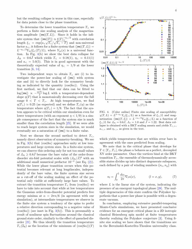
but the resulting collapse is worse in this case, especiallyfor data points close to the phase transition.

To determine the lower transition temperature T<

weperform a finite size scaling analysis of the magnetiza-tion amplitude h|m|(T, L)i. Since it holds in the infi-

nite system that h|m|(T )i / ⇠(T )�⌘</2<

with correlationlength ⇠

<

= exp�a<

pT<

/pT<

� T�and non-universal

factor a<

, it follows for a finite system that h|m|(T, L)i =L�⌘</2Y

m

(⇠<

(T )/L), where Ym

(x) is a universal func-tion. In Fig. 4(b) we show the best data collapse forJth

= 0.6J which yields T<

= 0.18(1), ⌘<

= 0.11(1)and a

<

= 5.0(5). This is in good agreement with thetheoretically expected value of ⌘

<

= 1/9 at the lowertransition [6, 14].

Two independent ways to obtain T<

are (i) to in-vestigate the power-law scaling of h|m|i with systemsize and (ii) to directly look for the symmetry break-ing as indicated by the quantity hcos(6↵)i. Using thefirst method, we find that our data can be fitted tologh|m|i / �⌘(T )

2 logL with a temperature-dependentslope ⌘(T ) that is monotonically decreasing over the fullrange 0 < T < T

>

. At high temperatures, we find⌘(T

>

) ' 0.25 (as expected) and we define T<

(⌘) as thetemperature where ⌘(T

<

) = 1/9. The fact that the sys-tem appears to be critical within our simulation even forlower temperatures (with an exponent ⌘ < 1/9) is a sim-ple consequence of the fact that the system size is muchsmaller than the correlation length [25]. If we were ableto reach larger system sizes in the simulation, we wouldeventually see a saturation of h|m|i to a finite value.

Next we discuss the second method to detect T<

,namely direct observation of symmetry-breaking. We seein Fig. 3(b) that hcos(6↵i approaches unity at low tem-peratures and large system sizes. In a finite-size system,we can observe this ordering only for not too small valuesof J

th

� 0.8J because the bare value of the order-from-disorder six-fold potential scales with (J

th

/J)6 with anadditional small numerical prefactor 10�4 (see Eq. (2)).While the lower phase transition occurs when this po-tential becomes relevant at long lengthscales, indepen-dently of the bare value, the finite system size servesas a cut-o↵ of the scaling making an e↵ect of the po-tential only visible at su�ciently large bare values. Toextract the transition temperature T

<

from hcos(6↵)i wehave to take into account that while at low temperaturesthe Gaussian order-from-disorder potential predicts freeenergy minima at ↵ = 2⇡n/6 (in agreement with oursimulation), at intermediate temperatures we observe inthe finite size system a tendency of the spins to prefera relative direction corresponding to a negative value ofhcos(6↵)i (see inset in Fig. 3(b)). This is presumably aresult of nonlinear spin fluctuations around the classicalground state order, similarly to the e↵ect of quenched dis-order [21]. We thus identify the transition temperatureT<

(Z6) as the location of the minimum of hcos(6↵)i(T )

FIG. 4. (Color online) Finite size scaling of susceptibility�(T, L) = L2�⌘>Y�(⇠>/L) as a function of ⇠>/L and mag-netization h|m|(T, L)i = L�⌘</2Ym(⇠</L) as a function of⇠</L for Jth = 0.6J , Jtt = 1.0 and J = 1.22. Best data col-lapse is obtained with a BKT scaling ansatz and yields T<,>,a<,> and ⌘<,> as given in the text.

which yields temperatures that are within error bars inagreement with the ones predicted from scaling.We note that in the critical phase that develops for

T 2 [T<

, T>

], the phase ↵ behaves as a perfect, decoupledXY order parameter. Once the vortices bind at the BKTtransition T

>

, the ensemble of thermodynamically acces-sible states divides up into distinct degenerate subspaces,each defined by a pair of winding numbers {n

x

, ny

} with

nl

=

ZL

0

dxl

2⇡r

l

↵(x), (l = x, y), (7)

where L is the linear size of the system, indicating thepresence of an emergent topological phase [28]. The mul-tiple degeneracies of this state confirm the Polyakov hy-pothesis that a power-law phase is possible with a degen-erate vacuum.In conclusion, employing extensive parallel-tempering

Monte-Carlo simulations, we have presented conclusiveevidence for an emergent critical phase in a 2D isotropicclassical Heisenberg spin model at finite temperaturesthereby realizing the Polyakov conjecture [3]. Using fi-nite size scaling we have shown that the transitions arein the Berezinskii-Kosterlitz-Thouless universality class.

5

At low temperatures, we find direct evidence of long-range order in the relative orientation of the spins viabreaking of a discrete six-fold symmetry induced by anorder-from-disorder potential. Direct numerical analysisof the spin sti↵ness tensor, the metric of the associatedSO(3) ⇥ U(1) topological manifold, and its Ricci flowwill be the topic of future work.

We acknowledge helpful discussions with B. Altshuler,K. Damle, J. Schmalian, M. D. Schulz, S. Trebst, andC. Weber. The Young Investigator Group of P.P.O. re-ceived financial support from the “Concept for the Fu-ture” of the Karlsruhe Institute of Technology (KIT)within the framework of the German Excellence Initia-tive. This work was supported by DOE grant DE-FG02-99ER45790 (P. Coleman) and P.C. and P.C. acknowl-edge visitors’ support from the Institute for the Theoryof Condensed Matter, Karlsruhe Institute of Technol-ogy (KIT). This work was carried out using the compu-tational resource bwUniCluster funded by the Ministryof Science, Research and Arts and the Universities ofthe State of Baden-Wurttemberg, Germany, within theframework program bwHPC.

[1] A. M. Polyakov, Gauge fields and strings, Contemporaryconcepts in physics, Vol. 3 (Harwood Academic Publish-ers, Chur, Switzerland, 1987).

[2] J. Zinn-Justin, Quantum Field Theory and Critical Phe-nomena (Oxford University Press, New York, NY, USA,2002).

[3] A. M. Polyakov, Phys. Lett. B 59, 79 (1975).[4] P. P. Orth, P. Chandra, P. Coleman, and J. Schmalian,

Phys. Rev. Lett. 109, 237205 (2012).[5] P. P. Orth, P. Chandra, P. Coleman, and J. Schmalian,

Phys. Rev. B 89, 094417 (2014).[6] J. Cardy, J. Phys. A: Math. Gen. 13, 1507 (1980).[7] G.-W. Chern, P. Mellado, and O. Tchernyshyov, Phys.

Rev. Lett. 106, 207202 (2011).[8] G.-W. Chern and O. Tchernyshyov, Phil. Trans. R. Soc.

A 370, 5718 (2012).[9] P. Chandra, P. Coleman, and A. I. Larkin, Phys. Rev.

Lett. 64, 88 (1990).[10] R. M. Fernandes, L. H. VanBebber, S. Bhattacharya,

P. Chandra, V. Keppens, D. Mandrus, M. A. McGuire,B. C. Sales, A. S. Sefat, and J. Schmalian, Phys. Rev.Lett. 105, 157003 (2010).

[11] R. M. Fernandes, A. V. Chubukov, J. Knolle, I. Eremin,and J. Schmalian, Phys. Rev. B 85, 024534 (2012).

[12] C. Weber, L. Capriotti, G. Misguich, F. Becca, M. Elha-jal, and F. Mila, Phys. Rev. Lett. 91, 177202 (2003).

[13] L. Capriotti, A. Fubini, T. Roscilde, and V. Tognetti,Phys. Rev. Lett. 92, 157202 (2004).

[14] J. V. Jose, L. P. Kadano↵, S. Kirkpatrick, and D. R.Nelson, Phys. Rev. B 16, 1217 (1977).

[15] Y. Miyatake, M. Yamamoto, J. J. Kim, M. Toyonaga,and O. Nagai, J. Phys. C 19, 2539 (1986).

[16] E. Marinari and G. Parisi, EPL 19, 451 (1992).[17] K. Hukushima and K. Nemoto, J. Phys. Soc. Jpn. 65,

1604 (1996).[18] B. Jeevanesan and P. P. Orth, Phys. Rev. B 90, 144435

(2014).[19] J. Villain, J. Phys France 38, 385 (1977).[20] E. Shender, Sov. Phys. JETP 56, 178 (1982).[21] C. L. Henley, Phys. Rev. Lett. 62, 2056 (1989).[22] J. T. Chalker, P. C. W. Holdsworth, and E. F. Shender,

Phys. Rev. Lett. 68, 855 (1992).[23] The Supplemental Material contains details on the

derivation of the order from disorder potential.[24] M. Challa and D. Landau, Phys. Rev. B 33, 437 (1986).[25] S. V. Isakov and R. Moessner, Phys. Rev. B 68, 104409

(2003).[26] C. C. Price and N. B. Perkins, Phys. Rev. Lett. 109,

187201 (2012).[27] C. Price and N. B. Perkins, Phys. Rev. B 88, 024410

(2013).[28] J. M. Kosterlitz and D. J. Thouless, J. Phys. C: Solid St.

Phys. 6, 1181 (1973).

Supplemental to “Emergent Power-Law Phase in the 2D Heisenberg WindmillAntiferromagnet: A Computational Experiment”

Bhilahari Jeevanesan,1 Premala Chandra,2 Piers Coleman,2, 3 and Peter P. Orth1, 4

1Institute for Theory of Condensed Matter, Karlsruhe Institute of Technology (KIT), 76131 Karlsruhe, Germany2Center for Materials Theory, Rutgers University, Piscataway, New Jersey 08854, USA

3Hubbard Theory Consortium and Department of Physics,Royal Holloway, University of London, Egham, Surrey TW20 0EX, UK

4School of Physics and Astronomy, University of Minnesota, Minneapolis, Minnesota 55455, USA(Dated: June 11, 2015)

Analytic calculation of the order-by-disorder potential

In this appendix we summarize our calculation of the order-by-disorder potential terms. The aim of this calculationis to determine the dependence of the free-energy on the manifold of ground-state configurations (the calculationfollows [1–3],[4]). In order to carry out the calculation we parametrize the spins as small fluctuations around oneof the ground states. We choose the plane of spins of the triangular lattice spins in their groundstate to lie in thexy plane. The honeycomb spins have an order parameter, that is described by angles � and ↵. The fluctuations ofthe triangular sublattice spins are called (⇢,�, ⌧) and those of the honeycomb spins are called (µ, ⌫). We choose thefollowing parametrization of the fluctuations

nA =

0

@1� ⇢

2y+⇢

2z

2⇢y

⇢z

1

A

nB = R

0

@1� �

2y+�

2z

2�y

�z

1

A =

0

B@� 1

2 �p32 �y +

�

2y+�

2z

4p32 � 1

2�y �p34 (�2

y

+ �2z

)�z

1

CA

nC = R2

0

@1� ⌧

2y+⌧

2z

2⌧y

⌧z

1

A =

0

B@� 1

2 +p32 ⌧y +

⌧

2y+⌧

2z

4

�p32 � 1

2⌧y +p34 (⌧2

y

+ ⌧2z

)⌧z

1

CA

hA =

✓1� µ2

1 + µ22

2

◆h0 + µ1� + µ2↵

hB = �✓

1� ⌫21 + ⌫222

◆h0 + ⌫1� + ⌫2↵

�

with unit vectors

h0 =

0

@sin� cos↵sin� sin↵

cos�

1

A , � =

0

@cos� cos↵cos� sin↵

sin�

1

A , ↵ =

0

@� sin↵cos↵0

1

A

and where R = Rz

(2⇡/3) is the rotation matrix that rotates spins around the z-axis by 2⇡/3. With this parametriza-tion it is a straightforward task to rewrite the Hamiltonian in the following form. The triangular spin Hamiltonianbecomes

Ht

= Jtt

X

i

nA

i

·

0

@X

j(i)

nB

j

+X

j(i)

nC

j

1

A+ Jtt

X

i

nB

i

·X

j(i)

nC

j

here the notation j(i) denotes summation over the neighbors j of the spin with index i. This is

Ht

= �3

2NJ

tt

+ �Ht

7

with

�Ht

= Jtt

X

hi,ji

1

4

�⇢2iy

+ ⇢2iz

+ �2jy

+ �2jz

�� 1

2⇢iy

�jy

+ ⇢iz

�jz

�

+Jtt

X

hi,ji

1

4

�⇢2iy

+ ⇢2iz

+ ⌧2jy

+ ⌧2jz

�� 1

2⇢iy

⌧jy

+ ⇢iz

⌧jz

�

+Jtt

X

hi,ji

1

4

��2iy

+ �2iz

+ ⌧2jy

+ ⌧2jz

�� 1

2�iy

⌧jy

+ �iz

⌧jz

�,

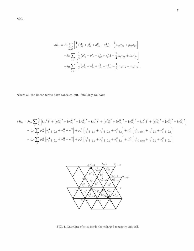
where all the linear terms have canceled out. Similarly we have

�Hh

= Jhh

X

i

3

2

h�µA

i1

�2+�µA

i2

�2+�⌫Ai1

�2+�⌫Ai2

�2+�µB

i1

�2+�µB

i2

�2+�⌫Bi1

�2+�⌫Bi2

�2+�µC

i1

�2+�µC

i2

�2+�⌫Ci1

�2+�⌫Ci2

�2i

�Jhh

X

i

µA

i1

h⌫Ai+1+2,1

+ ⌫Bi1 + ⌫C

i1

i+ µB

i1

h⌫Ai+1+2,1

+ ⌫Bi+1+2,1

+ ⌫Ci+1,1

i+ µC

i1

h⌫Ai+1+2,1

+ ⌫Bi+2,1

+ ⌫Ci+1+2,1

i

�Jhh

X

i

µA

i2

h⌫Ai+1+2,2

+ ⌫Bi2 + ⌫C

i2

i+ µB

i2

h⌫Ai+1+2,2

+ ⌫Bi+1+2,2

+ ⌫Ci+1,2

i+ µC

i2

h⌫Ai+1+2,2

+ ⌫Bi+2,2

+ ⌫Ci+1+2,2

i

FIG. 1. Labelling of sites inside the enlarged magnetic unit-cell.

8

and finally

Hth = Jth

X

i

cos↵⇢iy

⇣µA

i2 + µB

i�1�2,2+ µC

i�1�2,2

⌘+ cos� sin↵⇢

iy

⇣µA

i1 + µB

i�1�2,1+ µC

i�1�2,1

⌘

� sin�⇢iz

⇣µA

i1 + µB

i�1�2,1+ µC

i�1�2,1

⌘� cos↵⇢

iy

�⌫Ai2 + ⌫B

i2 + ⌫Ci2

�� cos� sin↵⇢

iy

�⌫Ai1 + ⌫B

i1 + ⌫Ci1

�

+sin�⇢iz

�⌫Ai1 + ⌫B

i1 + ⌫Ci1

�+ J

th

X

i

p3 sin↵� cos↵

2�iy

⇣µA

i2 + µB

i2 + µC

i�2,2

⌘

�p3 cos↵+ sin↵

2cos��

iy

⇣µA

i1 + µB

i1 + µC

i�2,1

⌘� sin��

iz

⇣µB

i1 + µA

i1 + µC

i�2,1

⌘

+�p3 sin↵+ cos↵

2�iy

⇣⌫Ai+1+2,2

+ ⌫Bi2 + ⌫C

i+1,2

⌘+

p3 cos↵+ sin↵

2cos��

iy

⇣⌫Ai+1+2,1

+ ⌫Bi1 + ⌫C

i+1,1

⌘

+sin��iz

⇣⌫Ai+1+2,1

+ ⌫Bi1 + ⌫C

i+1,1

⌘+ J

th

X

i

�p3 sin↵+ cos↵

2⌧iy

⇣µA

i2 + µB

i�1,2+ µC

i2

⌘

+

p3 cos↵� sin↵

2cos�⌧

iy

⇣µA

i1 + µB

i�1,1+ µC

i1

⌘� sin�⌧

iz

⇣µA

i1 + µB

i�1,1+ µC

i1

⌘

+

p3 sin↵+ cos↵

2⌧iy

⇣⌫Ai+1+2,2

+ ⌫Bi+2,2

+ ⌫Ci2

⌘�

p3 cos↵� sin↵

2cos�⌧

iy

⇣⌫Ai+1+2,1

+ ⌫Bi+2,1

+ ⌫Ci1

⌘

+sin�⌧iz

⇣⌫Ai+1+2,1

+ ⌫Bi+2,1

+ ⌫Ci1

⌘.

We transform this into fourier space with

⇢i

= ⇢ (ri

) =1

(2⇡)2

Zd2qeiqri⇢(q)

and rewrite the resulting total Hamiltonian in matrix form. This matrix has dimensions 18 ⇥ 18. It may, however,be written in extremely compact block form. This will facilitate the calculation of the free energy below. The fullHamiltonian is

�H =N

6(2⇡)2

Zd2q †

✓Jtt

Mt

Jth

M†th

Jth

Mth

Jhh

Mh

◆ .

with

Mt

=

152 I� j0j

†0

2 00 3I+ j0j

†0

!

Mh

=

0

BB@

3I �ei(q1+q2)j†0 0 0�e�i(q1+q2)j0 3I 0 0

0 0 3I �ei(q1+q2)j†00 0 �e�i(q1+q2)j0 3I

1

CCA

and

Mth

=

0

BB@

j0u j0v

�j†0u �j†0vj0w 0�j†0w 0

1

CCA .

9

The entries are themselves matrices:

j0 =

0

@1 1 1

ei(q1+q2) 1 eiq1

ei(q1+q2) eiq2 1

1

A

u = cos�

0

@sin↵ 0 00 sin(↵+ 4⇡

3 ) 00 0 sin(↵+ 2⇡

3 )

1

A

v = � sin�

0

@1 0 00 1 00 0 1

1

A

w =

0

@cos↵ 0 00 cos(↵+ 4⇡

3 ) 00 0 cos(↵+ 2⇡

3 )

1

A .

The quantity describing the fluctuation amplitudes is given by

(Q1, Q2) =�⇢y

,�y

, ⌧y

, ⇢z

,�z

, ⌧z

, µA

1 , µB

1 , µC

1 , ⌫A

1 , ⌫B1 , ⌫C1 , µA

2 , µB

2 , µC

2 , ⌫A

2 , ⌫B2 , ⌫C2�.

Finally, the correction to the free energy due to the fluctuations in a given ground state, characterized by � and ↵, iscomputed by the formula

�F = T

Zd2q log�

with determinant

� = det

✓Jtt

Mt

Jth

M†th

Jth

Mth

Jhh

Mh

◆.

A straightforward analytical evaluation of this determinant is complicated by the large dimension of the matrices.However, we may still carry out this computation by making repeated use of the block structure of �H. We use thefollowing block matrix decomposition:

✓A BC D

◆=

✓1 00 D

◆✓A B

D�1C 1

◆=

✓1 00 D

◆✓1 B0 1

◆✓A�BD�1C 0

D�1C 1

◆.

Since all three matrices are triangular, the determinant is just

det

✓A BC D

◆= detD det

�A�BD�1C

�,

an equality known as the Schur identity. Iterative application of this identity to the block matrices breaks the blockstructure down, until we are left with a determinant of a 3⇥3 matrix. We start with the calculation of the determinantfor the special case � = ⇡

2 . Here the determinant (after discarding ↵-independent factors) can be written as

3X

n=0

�n

✓Jth

J

◆2n

with J =pJtt

Jhh

and q-dependent �n

. Computation of the �n

shows that only n = 3 yields an ↵-dependence. Thetwo other determinants are independent of ↵ and are therefore not responsible for the selection of the groundstate.Integration over q yields the sought free energy dependence on ↵. Numerical evaluation of this last integral yields

�F ⌘✓Jth

J

◆6NT

3

Zd2q

(2⇡)2�3

�0= �10�4NT cos2(3↵)

✓Jth

J

◆6

.

10

Next we compute to lowest-order in�Jth

J

�the dependence on �. In computing the determinant by Schur’s identity,

one is left with a determinant of the form

log det

"I+

✓Jth

J

◆2

A�1B +

✓Jth

J

◆4

A�1C

#,

where A,B,C are 3 ⇥ 3 matrices. We are only interested in the lowest-order correction, which will obviously be

proportional to�Jth

J

�2. We find this most conveniently by rewriting the logarithm as a trace:

log det

"I+

✓Jth

J

◆2

A�1B +

✓Jth

J

◆4

A�1C

#= Tr[log(I+

✓Jth

J

◆2

A�1B +

✓Jth

J

◆4

A�1C)] ⌘X

Tn

✓Jth

J

◆2n

Once the Tn

are known, the free energy can be expressed as

�F ⌘6X

n=1

�Fn

✓Jth

J

◆2n

=NT

3

6X

n=1

✓Jth

J

◆2n Zd2q

(2⇡)2Tn

Next we compute the Tn

by expanding the logarithm in�Jth

J

�2

Tr[log(I+✓Jth

J

◆2

A�1B +

✓Jth

J

◆4

A�1C)] =1X

1

(�)n�1

�Jth

J

�2nTrh(A�1B +

�Jth

J

�2A�1C)n

i

n

with

T1 = Tr⇥A�1B

⇤

T2 = Tr⇥A�1C

⇤� 1

2Tr⇥(A�1B)2

⇤

T3 = �Tr⇥A�1BA�1C

⇤+

1

3Tr⇥(A�1B)3

⇤.

Here we will only require T1. Using the stated formula, it is straightforward to calculate the lowest-order dependenceof the free energy on �. We find

�F = 0.131274 cos(2�)NT

✓Jth

J

◆2

.

[1] J. Villain, J. Phys France 38, 385 (1977).[2] E. Shender, Sov. Phys. JETP 56, 178 (1982).[3] C. L. Henley, Phys. Rev. Lett. 62, 2056 (1989).[4] J. T. Chalker, P. C. W. Holdsworth, and E. F. Shender, Phys. Rev. Lett. 68, 855 (1992).