comparison of computational results with a low-g nitrogen ... · comparison of computational...

American Institute of Aeronautics and Astronautics

1

Comparison of Computational Results with a Low-g,

Nitrogen Slosh and Boiling Experiment

Mark. E. M. Stewart1

VPL at NASA Glenn Research Center, Cleveland, Ohio, 44135

Jeffrey P. Moder2

NASA Glenn Research Center, Cleveland, Ohio, 44135

This paper compares a fluid/thermal simulation, in Fluent, with a low-g, nitrogen slosh

and boiling experiment. In 2010, the French Space Agency, CNES, performed cryogenic

nitrogen experiments in a low-g aircraft campaign. From one parabolic flight, a low-g

interval was simulated that focuses on low-g motion of nitrogen liquid and vapor with

significant condensation, evaporation, and boiling. The computational results are compared

with high-speed video, pressure data, heat transfer, and temperature data from sensors on

the axis of the cylindrically shaped tank. These experimental and computational results

compare favorably. The initial temperature stratification is in good agreement, and the

two-phase fluid motion is qualitatively captured. Temperature data is matched except that

the temperature sensors are unable to capture fast temperature transients when the sensors

move from wet to dry (liquid to vapor) operation. Pressure evolution is approximately

captured, but condensation and evaporation rate modeling and prediction need further

theoretical analysis.

Nomenclature

a, acg = acceleration, acceleration of center of gravity, m/s2

ALAT = Air Liquide Advanced Technology

CNES = Centre National d’Etudes Spatiales

Cp, Cv = specific heat at constant pressure and constant volume, J/kg-K

c = VOF fraction, unitless

g = gravitational acceleration, m/s2

k = thermal conductivity, W/m-K

MW = molecular weight, kg/kmol

m = mass flux due to evaporation (>0) and condensation, kg/s-m2

P, Psat(T) = static pressure, Pa, saturation pressure at temperature, Pa

Ru = universal gas constant, J/kmol-K

r

= radius vector from center of gravity, m

T, Tsat(P) = temperature, K, saturation temperature at pressure, K

UDF = User Defined Function (Fluent)

VOF = Volume of Fluid

V, vr = fluid velocity, m/s, radial velocity relative to center of gravity, m/s

w = dissipation per unit turbulent kinetic energy, 1/s

Z = compressibility factor, unitless

Δt = time step, s

= surface tension, N/m

= turbulent kinetic energy, m2/s

2

= molecular viscosity, Pa s

= density, kg/m3

1 Senior Research Engineer, MS VPL-3, AIAA member.

2 Research Aerospace Engineer, Engine Combustion Branch, MS 5-10, AIAA Member.

https://ntrs.nasa.gov/search.jsp?R=20150018267 2019-05-04T14:31:19+00:00Z


2

Figure 1. Cross-sectional geometry for

experimental apparatus. Picture from

Mathey et al. [1].

cond, evap = accommodation coefficients for condensation and evaporation, unitless

τ = time constant for temperature sensor, s

, = angular velocity vector, rad/s, angular acceleration vector, rad/s

2

liq, vap = subscripts indicating liquid and vapor phases

I. Introduction

N 2010, Centre National d’Etudes Spatiales and Air Liquide Advanced Technologies conducted a parabolic flight

campaign which included an experimental test bench, Cry0genic, to study nitrogen sloshing and boiling in low-g

conditions. Computational fluid dynamics simulations accompanied these experiments [1] [2]. This experimental

and computational work is part of a long term effort by CNES to examine cryogenic fluid behavior in low-g

conditions, including evaporation, condensation, boiling, stratification, pressurization and de-pressurization, as well

as helium pressurization.

CNES is interested [3] in cryogenic fluid behavior in flight conditions, gathering data for validating

computational simulations, and predicting tank pressure, thermal stratification, and tank outlet/engine inlet

conditions for engine restart after an orbital coast phase. NASA is interest in long term storage of cryogenic

propellants for on-orbit refueling and long duration space missions. Cryogenic propellants promise higher specific

impulse than storable hypergolic fuels, but storage for long duration missions must be demonstrated. A pacing

technology for manned Mars missions using Nuclear Thermal Propulsion is storage of many tons of liquid hydrogen

propellant for several years with minimal boil-off loss. With this convergence of interests, NASA and CNES agreed

to benchmark simulations, and this is one of the test cases.

II. Geometry and Grid

The experimental apparatus consisted of nitrogen, gas and liquid, in a

sapphire cylindrical shell with aluminum and stainless steel (inox)

lids (Figure 1) all contained in an insulating vacuum chamber. To

remove the small residual heat fluxes into the vessel (and reduce boil

off), the lower lid contains a cryocooler. Instrumentation included

high speed video and twelve temperature sensors mounted to a post

along the axis of the shell. The dimensions of the cylindrical

nitrogen vessel are approximately 6 cm by 10 cm, with a slosh

frequency of near 4 Hz.

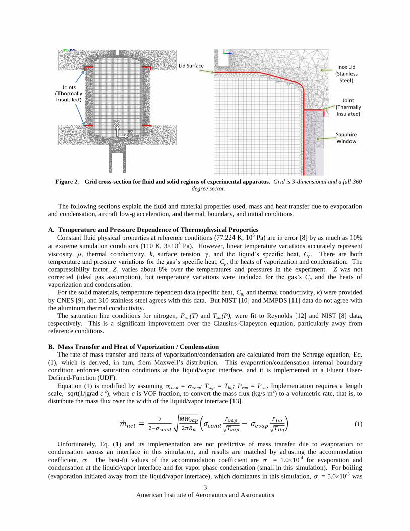
The three-dimensional grid is shown in Figure 2. It is a full 360-

degree sector of the apparatus with 569,110 fluid cells, and 685,858

solid cells. The solid grid is unstructured with variable resolution.

The interior of the fluid grid is a uniform, structured grid with ~1 mm

resolution, but near the fluid-solid interface, it becomes unstructured

and merges into the solid grid. The grid does not include the central

post where the fluid temperature sensors are mounted. The region of

the joints and sealing gaskets between the sapphire shell and metal

lids is meshed; however, thermal isolation is enforced along the

interface lines shown in Figure 2. The grid was partitioned to run of

16 or 32 processors.

III. Numerical Methods and Fluent Settings

ANSYS Fluent version 13 [4] was used to solve thermal equations in the solid coupled to thermal/fluid equations

in the fluid region. While the energy equation is solved in the solid region, mass, momentum, energy, and

turbulence equations are solved in the fluid region with second-order upwind schemes. The PISO scheme was used

for the pressure-velocity coupling, and the PRESTO! scheme was used for the pressure interpolation. The gas phase

was modeled as an ideal gas, and a Boussinesq approximation was used for the liquid phase. Two-phase flow was

resolved using the Volume of Fluid method [5]. The -w SST turbulence model of Menter [6] [7] was used with a

turbulent damping coefficient of 10. The simulation was time-accurate (second order implicit temporal scheme)

with a time step Δt = 1.010-4

seconds. The simulation was run on Pleiades at the NASA Advanced

Supercomputing Facility. Add execution time.

I

Cryocooler


3

Figure 2. Grid cross-section for fluid and solid regions of experimental apparatus. Grid is 3-dimensional and a full 360

degree sector.

The following sections explain the fluid and material properties used, mass and heat transfer due to evaporation

and condensation, aircraft low-g acceleration, and thermal, boundary, and initial conditions.

A. Temperature and Pressure Dependence of Thermophysical Properties

Constant fluid physical properties at reference conditions (77.224 K, 105 Pa) are in error [8] by as much as 10%

at extreme simulation conditions (110 K, 3105 Pa). However, linear temperature variations accurately represent

viscosity, , thermal conductivity, k, surface tension, , and the liquid’s specific heat, Cp. There are both

temperature and pressure variations for the gas’s specific heat, Cp, the heats of vaporization and condensation. The

compressibility factor, Z, varies about 8% over the temperatures and pressures in the experiment. Z was not

corrected (ideal gas assumption), but temperature variations were included for the gas’s Cp and the heats of

vaporization and condensation.

For the solid materials, temperature dependent data (specific heat, Cp, and thermal conductivity, k) were provided

by CNES [9], and 310 stainless steel agrees with this data. But NIST [10] and MMPDS [11] data do not agree with

the aluminum thermal conductivity.

The saturation line conditions for nitrogen, Psat(T) and Tsat(P), were fit to Reynolds [12] and NIST [8] data,

respectively. This is a significant improvement over the Clausius-Clapeyron equation, particularly away from

reference conditions.

B. Mass Transfer and Heat of Vaporization / Condensation

The rate of mass transfer and heats of vaporization/condensation are calculated from the Schrage equation, Eq.

(1), which is derived, in turn, from Maxwell’s distribution. This evaporation/condensation internal boundary

condition enforces saturation conditions at the liquid/vapor interface, and it is implemented in a Fluent User-

Defined-Function (UDF).

Equation (1) is modified by assuming cond = evap; Tvap = Tliq; Pvap = Psat. Implementation requires a length

scale, sqrt(1/|grad c|2), where c is VOF fraction, to convert the mass flux (kg/s-m

2) to a volumetric rate, that is, to

distribute the mass flux over the width of the liquid/vapor interface [13].

�̇�𝑛𝑒𝑡 = 2

2−𝜎𝑐𝑜𝑛𝑑√

𝑀𝑊𝑣𝑎𝑝

2𝜋𝑅𝑢(𝜎𝑐𝑜𝑛𝑑

𝑃𝑣𝑎𝑝

√𝑇𝑣𝑎𝑝− 𝜎𝑒𝑣𝑎𝑝

𝑃𝑙𝑖𝑞

√𝑇𝑙𝑖𝑞) (1)

Unfortunately, Eq. (1) and its implementation are not predictive of mass transfer due to evaporation or

condensation across an interface in this simulation, and results are matched by adjusting the accommodation

coefficient, . The best-fit values of the accommodation coefficient are = 1.010-4

for evaporation and

condensation at the liquid/vapor interface and for vapor phase condensation (small in this simulation). For boiling

(evaporation initiated away from the liquid/vapor interface), which dominates in this simulation, = 5.010-3

was


4

Figure 4. Initial temperature determined from a

transient simulation of the high-g interval. Temperature

sensor locations are also marked. Liquid/vapor interface

indicated between sensors t12c and t12e. High temperature

gradient near t12b.

Figure 3. Acceleration profile during low-g interval. High-g refers

to the preceding and following intervals.

used. This boiling model includes a superheat criterion, Tmax – Tsat(P) > 5 K, that is, the liquid temperature within

the cell must exceed the saturation temperature by a fixed temperature in the liquid phase. Tmax is the maximum

temperature in the cell, including adjacent walls. The vapor phase condensation model includes a similar

supercooled liquid criteria based on the minimum temperature.

Data exists for boiling heat transfer rates for 1-g, nitrogen boiling in wires [14] and cylinders [15]; however, this

wire and cylinder data is not clearly applicable here, so they can only provide guidance.

C. Non-Inertial Reference Frame Accounts for Low-g Aircraft Acceleration

A non-inertial reference frame will

account for the acceleration of the aircraft

during low-g (and high-g) parabolic flight.

In the general case, such as a satellite with

measured linear acceleration, cga

, angular

velocity,

, and angular acceleration,

,

the acceleration components are given by

Eq. (2). The terms included on the RHS of

the x-, y-, and z-momentum equations are

a

, and in the energy equation, Va

.

In this experiment, angular velocity and

acceleration are zero. Only two

components of the linear acceleration of the

aircraft, ax and az, were measured, and ay is

assumed to be zero. The acceleration

components were measured during

parabolic flight at a 10 Hz sampling rate, as

shown in Figure 3. Values are interpolated

as piece-wise linear fits. The steady initial

conditions assumed in the high-g phase of parabolic flight are ax = -16.5 m/s2 and az = -1.93 m/s

2.

)(2 rrvaa rcg

(2)

The Bond or Eötvös number is in the range [0.3, 6.]

during the low-g phase, and it is approximately 1 for

about 10 seconds.

The weightless interval of parabolic flight is referred

to as low-g, while high-g refers to the intervening

interval.

D. Thermal, Boundary, and Initial Conditions

Despite being contained in a vacuum chamber, small

heat fluxes exist into the experimental apparatus, and

they are compensated by a cryocooler attached to the

lower aluminum lid. The surface heat fluxes are due to

radiation from the vacuum chamber inner surface, and

conduction through the near vacuum conditions.

Consequently, heat flows through the apparatus as

discussed in the next section. The cryocooler removes

about 4 W, and the surface heat inflow is estimated and

assumed to be uniformly distributed over the top lid (1

W), bottom lid (1 W), and the sapphire surface (2 W).

Nitrogen fills the tank 55% full. The liquid-to-

vapor contact angle is taken as 5 degrees. Between low-

g intervals in the parabolic flight, the conditions are


5

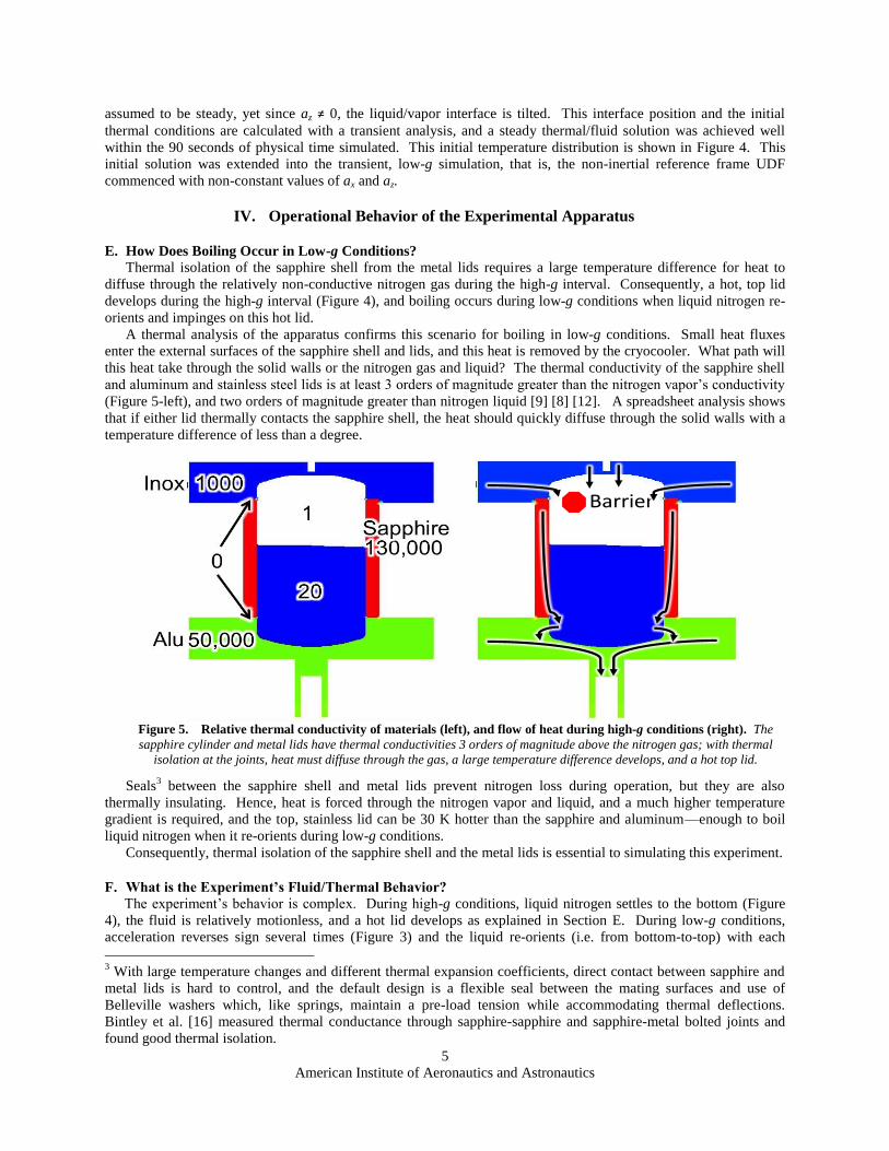
Figure 5. Relative thermal conductivity of materials (left), and flow of heat during high-g conditions (right). The

sapphire cylinder and metal lids have thermal conductivities 3 orders of magnitude above the nitrogen gas; with thermal

isolation at the joints, heat must diffuse through the gas, a large temperature difference develops, and a hot top lid.

Barrier

assumed to be steady, yet since az ≠ 0, the liquid/vapor interface is tilted. This interface position and the initial

thermal conditions are calculated with a transient analysis, and a steady thermal/fluid solution was achieved well

within the 90 seconds of physical time simulated. This initial temperature distribution is shown in Figure 4. This

initial solution was extended into the transient, low-g simulation, that is, the non-inertial reference frame UDF

commenced with non-constant values of ax and az.

IV. Operational Behavior of the Experimental Apparatus

E. How Does Boiling Occur in Low-g Conditions?

Thermal isolation of the sapphire shell from the metal lids requires a large temperature difference for heat to

diffuse through the relatively non-conductive nitrogen gas during the high-g interval. Consequently, a hot, top lid

develops during the high-g interval (Figure 4), and boiling occurs during low-g conditions when liquid nitrogen re-

orients and impinges on this hot lid.

A thermal analysis of the apparatus confirms this scenario for boiling in low-g conditions. Small heat fluxes

enter the external surfaces of the sapphire shell and lids, and this heat is removed by the cryocooler. What path will

this heat take through the solid walls or the nitrogen gas and liquid? The thermal conductivity of the sapphire shell

and aluminum and stainless steel lids is at least 3 orders of magnitude greater than the nitrogen vapor’s conductivity

(Figure 5-left), and two orders of magnitude greater than nitrogen liquid [9] [8] [12]. A spreadsheet analysis shows

that if either lid thermally contacts the sapphire shell, the heat should quickly diffuse through the solid walls with a

temperature difference of less than a degree.

Seals3 between the sapphire shell and metal lids prevent nitrogen loss during operation, but they are also

thermally insulating. Hence, heat is forced through the nitrogen vapor and liquid, and a much higher temperature

gradient is required, and the top, stainless lid can be 30 K hotter than the sapphire and aluminum—enough to boil

liquid nitrogen when it re-orients during low-g conditions.

Consequently, thermal isolation of the sapphire shell and the metal lids is essential to simulating this experiment.

F. What is the Experiment’s Fluid/Thermal Behavior?

The experiment’s behavior is complex. During high-g conditions, liquid nitrogen settles to the bottom (Figure

4), the fluid is relatively motionless, and a hot lid develops as explained in Section E. During low-g conditions,

acceleration reverses sign several times (Figure 3) and the liquid re-orients (i.e. from bottom-to-top) with each

3 With large temperature changes and different thermal expansion coefficients, direct contact between sapphire and

metal lids is hard to control, and the default design is a flexible seal between the mating surfaces and use of

Belleville washers which, like springs, maintain a pre-load tension while accommodating thermal deflections.

Bintley et al. [16] measured thermal conductance through sapphire-sapphire and sapphire-metal bolted joints and

found good thermal isolation.


6

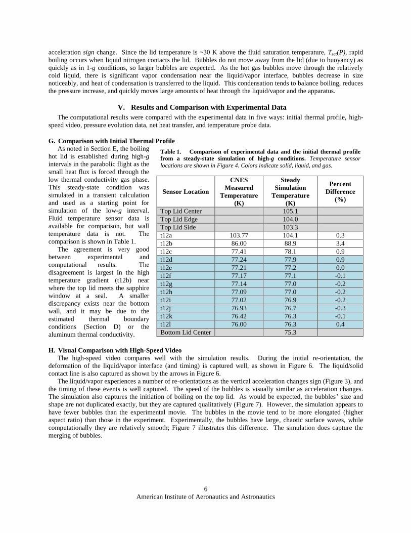
Table 1. Comparison of experimental data and the initial thermal profile

from a steady-state simulation of high-g conditions. Temperature sensor

locations are shown in Figure 4. Colors indicate solid, liquid, and gas.

Sensor Location

CNES

Measured

Temperature

(K)

Steady

Simulation

Temperature

(K)

Percent

Difference

(%)

Top Lid Center 105.1

Top Lid Edge 104.0

Top Lid Side 103.3

t12a 103.77 104.1 0.3

t12b 86.00 88.9 3.4

t12c 77.41 78.1 0.9

t12d 77.24 77.9 0.9

t12e 77.21 77.2 0.0

t12f 77.17 77.1 -0.1

t12g 77.14 77.0 -0.2

t12h 77.09 77.0 -0.2

t12i 77.02 76.9 -0.2

t12j 76.93 76.7 -0.3

t12k 76.42 76.3 -0.1

t12l 76.00 76.3 0.4

Bottom Lid Center 75.3

acceleration sign change. Since the lid temperature is ~30 K above the fluid saturation temperature, Tsat(P), rapid

boiling occurs when liquid nitrogen contacts the lid. Bubbles do not move away from the lid (due to buoyancy) as

quickly as in 1-g conditions, so larger bubbles are expected. As the hot gas bubbles move through the relatively

cold liquid, there is significant vapor condensation near the liquid/vapor interface, bubbles decrease in size

noticeably, and heat of condensation is transferred to the liquid. This condensation tends to balance boiling, reduces

the pressure increase, and quickly moves large amounts of heat through the liquid/vapor and the apparatus.

V. Results and Comparison with Experimental Data

The computational results were compared with the experimental data in five ways: initial thermal profile, high-

speed video, pressure evolution data, net heat transfer, and temperature probe data.

G. Comparison with Initial Thermal Profile

As noted in Section E, the boiling

hot lid is established during high-g

intervals in the parabolic flight as the

small heat flux is forced through the

low thermal conductivity gas phase.

This steady-state condition was

simulated in a transient calculation

and used as a starting point for

simulation of the low-g interval.

Fluid temperature sensor data is

available for comparison, but wall

temperature data is not. The

comparison is shown in Table 1.

The agreement is very good

between experimental and

computational results. The

disagreement is largest in the high

temperature gradient (t12b) near

where the top lid meets the sapphire

window at a seal. A smaller

discrepancy exists near the bottom

wall, and it may be due to the

estimated thermal boundary

conditions (Section D) or the

aluminum thermal conductivity.

H. Visual Comparison with High-Speed Video

The high-speed video compares well with the simulation results. During the initial re-orientation, the

deformation of the liquid/vapor interface (and timing) is captured well, as shown in Figure 6. The liquid/solid

contact line is also captured as shown by the arrows in Figure 6.

The liquid/vapor experiences a number of re-orientations as the vertical acceleration changes sign (Figure 3), and

the timing of these events is well captured. The speed of the bubbles is visually similar as acceleration changes.

The simulation also captures the initiation of boiling on the top lid. As would be expected, the bubbles’ size and

shape are not duplicated exactly, but they are captured qualitatively (Figure 7). However, the simulation appears to

have fewer bubbles than the experimental movie. The bubbles in the movie tend to be more elongated (higher

aspect ratio) than those in the experiment. Experimentally, the bubbles have large, chaotic surface waves, while

computationally they are relatively smooth; Figure 7 illustrates this difference. The simulation does capture the

merging of bubbles.


7

Figure 6. Comparison of computational predictions (left) and experimental data (right) showing the liquid/vapor

interface as it rapidly deforms with the initial reduction in gravity. Arrows indicate the liquid/solid contact line. At left, the

blue bands indicate the sapphire/lid joints.

Figure 7. Comparison of computational predictions (left) and experimental data (right) showing the liquid/vapor interface

during the intense boiling phase. At left, the blue bands indicate the sapphire/lid joints.

I. Pressure Data

Pressure is a measure of the net mass transfer due to evaporation and condensation. Figure 8 (left) shows the

time evolution of mass transfer rate (evaporation, condensation, and net), and (right) shows pressure with time for

two accommodation coefficients. Evaporation (boiling) precedes condensation as the liquid nitrogen contacts the

top lid. After a surge of condensation and a pressure drop, evaporation and condensation reach an approximate

balance with no apparent correlation with subsequent re-orientations.

The computational results for pressure, shown in Figure 8, show general agreement with the experimentally

measured data. The simulation does capture the initial rapid pressure rise and reversal, but it does not capture the

gentle pressure rise between 97 and 107 seconds.

J. Heat Transfer Rate and Fluid Enthalpy Increase

We verify the boiling heat transfer rate by calculating the increase in fluid enthalpy in the simulation and

comparing with an estimate from the experiment. The results, shown in Figure 9, show good agreement, and

indicate the accommodation coefficient value, = 5.010-3

, used in Eq. (1) is a good fit. The computational

estimate evaluated the integral of Eq. (3), and the experimental estimate of enthalpy assumed the fluid was thermally

stratified at the temperatures indicated by the probes before and after the low-g interval.


8

Figure 8. Evaporation, condensation, and net mass transfer rates (left), and pressure evolution for two accommodation

coefficients compared with experimental measurements (right). The pale red line indicates acceleration, ax/g.

Figure 9. To check if the heat transfer rate is correct, compare the computationally measured change in fluid enthalpy

with an estimate from the experiment. The pale red line indicates acceleration, ax/g.

∫ 𝜌𝑙𝑖𝑞(𝑇 − 𝑇𝑟𝑒𝑓) 𝐶𝑣𝑙𝑖𝑞 𝑉𝑂𝐹𝑙𝑖𝑞

𝑣𝑜𝑙𝑑𝑉𝑜𝑙 (3)

K. Comparison of Temperature Probe Results

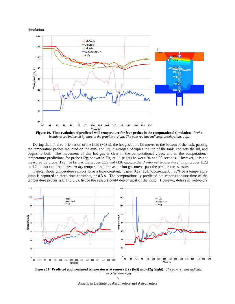
Although experimental wall temperature data were not available, predictions from the simulation are given in

Figure 10. From 114 to 120 seconds in Figure 10, the top lid is reheating. How long does the lid take to reheat

during the high-g interval? Combining Figure 10 data with the transient solution for initial conditions, the lid re-

heating time is expected to be completely reheated within 60 seconds.

The temperature evolution at two temperature probes is shown in Figure 11, and these are typical of the 12

probes. The results for probe t12a show the probe is in the hottest vapor at the top of the tank. As the hot vapor

moves away and is replaced with cold liquid, the predicted quick temperature drop agrees with the experimental

measurements. From 95 to 113 seconds, the liquid slowly heats, and there is general agreement between the two

results. However after 115 seconds, the computation predicts re-heating of the vapor near the lid, while the

experimental data do not show this. One explanation is that liquid nitrogen remains in the fill lines above probe

t12a, and this liquid drains over the temperature probe after the re-orientation. The fill lines are not modeled in the

cond = 2.10-4

cond = 1.10-4


9

Figure 11. Predicted and measured temperatures at sensors t12a (left) and t12g (right). The pale red line indicates

acceleration, ax/g.

Figure 10. Time evolution of predicted wall temperature for four probes in the computational simulation. Probe

locations are indicated by stars in the graphic at right. The pale red line indicates acceleration, ax/g.

simulation.

During the initial re-orientation of the fluid (~93 s), the hot gas at the lid moves to the bottom of the tank, passing

the temperature probes mounted on the axis, and liquid nitrogen occupies the top of the tank, contacts the lid, and

begins to boil. The movement of this hot gas is clear in the computational video, and in the computational

temperature predictions for probe t12g, shown in Figure 11 (right) between 94 and 95 seconds. However, it is not

measured by probe t12g. In fact, while probes t12a and t12b capture the dry-to-wet temperature jump, probes t12d

to t12l do not capture the wet-to-dry temperature jump as the hot gas moves past the temperature sensors.

Typical diode temperature sensors have a time constant, τ, near 0.1s [16]. Consequently 95% of a temperature

jump is captured in three time constants, or 0.3 s. The computationally predicted hot vapor exposure time of the

temperature probes is 0.3 to 0.5s, hence the sensors could detect most of the jump. However, delays in wet-to-dry


10

response time have been observed experimentally and analyzed [17]. The explanation is that wet-to-dry transition of

a diode sensor includes a liquid film that must vaporize before gas temperature is measured.

VI. Conclusion

The computational and experimentally results agree. The initial temperature profile, bubble motion, and heat

transfer, are in good agreement, while the pressure evolution, and shape and number of bubbles is only acceptable.

Evaporation/condensation model is not predictive of rates and more theoretical analysis is needed. Turbulence

damping keeps turbulence away from interface.

Acknowledgments

The authors thank Jason Hartwig, Mojib Hasan, Olga Kartuzova, and Juan Agui for helpful discussions. Steve

Barsi generated the grid, Nicole Velez handled many administrative issues, and Rich Rinehart provided graphics

expertise. The authors also thank Fabrice Mathey, Didier Zaepffel, and Sebastian Bianchi of ALAT for a valuable

benchmarking meeting. This work was conducted under an "Implementing Arrangement Between the National

Aeronautics and Space Administration of the United States of America and the Centre National D’Etudes Spatiales

of France on Cooperation Related to Benchmarking Activities Regarding Computational Propellant Management

Capability.” The authors would like to thank Benjamin Legrand, Vincent Leudiere, and Pascal Fortunier of CNES.

Without their help and discussions, this valuable cooperative activity would not have been possible. This work was

supported by the NASA Space Technology Mission Directorate's Technology Demonstration Missions Program

under the Evolvable Cryogenics Project.

References

[1] F. Mathey, C. Blanc-Mathieu, S. Demare, D. Zaepffel, B. Legrand and V. Leudiere, "Numerical Simulations of Two-Phase

Flow Inside Cryogenic Tanks Under Microgravity Conditions: Comparison with Experiments Onboard Zero-G Parabolic

Flights," in Space Propulsion Conference (Europe), Cologne, 2014.

[2] J. Lacapere, J. Tanchon, B. Legrand, Y. Prel and V. Leudiere, "Thermal Destratification Tests with Liquid Nitrogen in

Parabolic Flights," in 61st International Astronautical Congress, IAC-110.A2.3.3, 2010.

[3] B. Legrand, J. Lacapere and S. Bianchi, "New Technologies for Cryogenic Propellant Management for Next Generation

Launchers," in AIAA Space , AIAA 2012-5203, Pasadena, 2012.

[4] ANSYS, ANSYS Fluent User's Guide, Release 14.0, Canonsburg, PA: ANSYS, Inc., 2011.

[5] S. W. J. Welch and J. Wilson, "A volume of fluid based method for fluid flows with phase change," Journal of

Computational Physics, vol. 160, no. 2, pp. 662-682, 2000.

[6] F. R. Menter, "Two-Equation Eddy-Viscosity Turbulence Models for Engineering Applications," AIAA Journal, vol. 32, no.

8, pp. 1598-1605, August 1994.

[7] ANSYS, ANSYS FUENT Theory Guide, Release 14.0, Canonsburg, PA: ANSYS, 2011.

[8] NIST, "Thermophysical Properties of Fluid Systems," National Institute for Standards and Technology, 2011. [Online].

Available: http://webbook.nist.gov/chemistry/fluid. [Accessed January 2015].

[9] Private Communication with CNES, 2014.

[10] NIST, "Material Measurement Laboratory: Cryogenics Technologies Group," [Online]. Available:

http://cryogenics.nist.gov/MPropsMAY/materialproperties.htm. [Accessed 2015 April].

[11] Federal Aviation Administration, MMPDS-06, Metallic Materials Properties Development and Standardization, FAA, April

2011.

[12] W. C. Reynolds, Thermodynamic Properties in SI: graphs, tables and computational equations for 40 substances, Dept. of

Mech Eng, Stanford University, 1979.

[13] O. Kartuzova and M. Kassemi, "Modeling Interfacial Turbulent Heat Tansfer during Ventless Pressurization of a Large

Scale Cryogenic Storage Tank in Microgravity," in AIAA, 2011.

[14] K. Okuyama and Y. Iida, "Transient boiling heat transfer characteristics of nitrogen (bubble behavior and heat transfer rate

at stepwise heat generation)," Int. J. Heat Mass Transfer, vol. 33, no. 10, pp. 2065-2071, 1990.

[15] A. Sakurai, M. Shiotsu and K. Hata, "Boiling heat transfer characteristics for heat inputs with various increasing rates in

liquid nitrogen," Cryogenics, vol. 32, no. 5, pp. 421-429, 1992.

[16] D. Linenberger, E. Spellicy and R. Radebaugh, "Thermal Response Times of Some Cryogenic Thermometers," in


11

Temperature: Its Measurement an Control in Science and Industry, American Institute of Physics, 1982, pp. 1367-1372.

[17] E. Rame and G. A. Zimmerli, "Analysis of capillary drainage from a flat solid strip," Physics of Fluids, vol. 26, no. 062102,

2014.

[18] D. Bintley, A. L. Woodcraft and F. C. Gannaway, "Millikelvin thermal conductance measurements of compact rigid thermal

isolation joints using sapphire-sapphire contacts, and of copper and beryllium-copper demountable thermal contacts,"

Cryogenics, vol. 47, no. 5-6, pp. 333-342, 2007.

comparison of computational results with a low-g nitrogen ... · comparison of computational...

Documents