a comparison of two models for cognitive diagnosis
TRANSCRIPT
A Comparison of Two Models for Cognitive Diagnosis
January 2004 RR-04-02
ResearchReport
Duanli Yan
Russell Almond
Robert Mislevy
Research & Development


A Comparison of Two Models for Cognitive Diagnosis
Duanli Yan and Russell Almond
ETS, Princeton, NJ
Robert Mislevy
University of Maryland, College Park, MD
January 2004

Research Reports provide preliminary and limited dissemination of ETS research prior to publication. They are available without charge from:
Research Publications Office Mail Stop 7-R ETS Princeton, NJ 08541

Abstract
Diagnostic score reports linking assessment outcomes to instructional interventions are one of
the most requested features of assessment products. There is a body of interesting work done in
the last 20 years including Tatsuoka’s rule space method (Tatsuoka, 1983), Haertal and Wiley’s
binary skills model (Haertal, 1984; Haertal & Wiley, 1993), and Mislevy, Almond, Yan, and
Steinberg’s Bayesian inference network (Mislevy, Almond, Yan, & Steinberg, 1999). Recent
research has resulted in major breakthroughs for the use of a parametric IRT model for
performing skills diagnoses. Hartz, Roussos, and Stout (2002) have developed an identifiable
and flexible model called the fusion model.
This paper compares the fusion model and the Bayesian inference network in the design
and analysis of an assessment, including the Q-matrix, and then compares other related models,
including rule space, item response theory (IRT), and general multivariate latent class models.
The paper also attempts to characterize the kinds of problems for which each type of
measurement model is well-suited. A general Bayesian psychometric framework provides
common language, making it easier to appreciate the differences.
In addition, this paper explores some of the strengths and weaknesses of each approach
based on a comparative analysis of a cognitive assessment, the mixed number subtraction data
set. In this case, both the fusion model and Bayesian network approaches yield similar
performance characteristics and also seem to pick up on different characteristics.
Key words: Cognitive diagnosis, fusion model, binary skills model, latent class models, Bayesian
network, Markov chain Monte Carlo (MCMC)
i

Table of Contents
Page
Introduction..................................................................................................................................... 1
Evidence-centered Design .............................................................................................................. 2
An Example From Mixed Number Subtraction.............................................................................. 3
Q-matrix ........................................................................................................................... 4
Bayesian Psychometric Framework................................................................................................ 6
Proficiency Model: Bayesian Network ............................................................................ 8
Proficiency Model: Fusion Model.................................................................................. 10
Noisy-and Models.................................................................................................................. 12
Evidence Model: Bayesian Network .............................................................................. 15
Evidence Model: Fusion Model ..................................................................................... 16
Comparison of Models.................................................................................................................. 16
Empirical Comparisons................................................................................................................. 19
Model Fitting ......................................................................................................................... 19
Procedures ...................................................................................................................... 19
Discussion....................................................................................................................... 20
Estimation Results and Comparisons .................................................................................... 21
Diagnostic Results and Comparisons .................................................................................... 25
Conclusion .................................................................................................................................... 29
References..................................................................................................................................... 31
Notes ............................................................................................................................................. 33
ii

List of Tables
Page
Table 1. Original Q-matrix Skill Requirements for Fraction Items................................................ 5
Table 2. Some Bayesian Psychometric Models in the Bayesian Psychometric Framework ........ 17
Table 3. Equivalence Classes and Evidence Models .................................................................... 19
Table 4. Final Q-matrix for Fusion Model Skill Requirements for Fraction Items...................... 22
Table 5. Estimated Proportions of Skill Masters .......................................................................... 23
Table 6. Estimated Item Parameters From 3LC and Fusion Model ............................................. 24
Table 7. Fusion Model and Bayesian Network Classifications at 0.5 Level ................................ 26
Table 8. Fusion Model and Bayesian Network Classifications at (0.4, 0.6) Level ...................... 27
Table 9. Selected Examinee Responses ........................................................................................ 28
iii
Table of Figures
Page
Figure 1. Conceptual assessment framework (CAF). ..................................................................... 3
Figure 2. Psychometric model for the conceptual assessment framework. .................................... 8
Figure 3. The graphical representation of the student model for mixed number subtraction. ........ 9
Figure 4. Compensatory (and-gate) model. .................................................................................. 12
Figure 5. Compensatory model with probabilitistic inversion of the outputs............................... 13
Figure 6. Noisy-and model with probabilistic inversion of inputs. .............................................. 14
Figure 7. Full noisy-and model with inversion of both inputs and outputs. ................................. 14
iv
Introduction
One of the most interesting and requested features in educational assessment is cognitive
diagnostic score reports. Instead of assigning a single ability estimate to each examinee as in
typical item response theory (IRT) model-based summative assessments, cognitive diagnosis
model-based formative assessments partition the latent space multidimensionality into more fine-
grained, often discrete or dichotomous cognitive skills or latent attributes, and evaluate the
examinee with respect to his/her level of competence for each attribute. Another purpose of
model-based cognitive diagnosis is to evaluate the items in terms of their effectiveness in
measuring the intended constructs and identify the accuracy with which the attributes are being
measured; this information can be used in improving test construction. The results of the
cognitive structure of the test may also be useful to inform the standard setting process for the
examination.
Tatsuoka’s rule space method (Tatsuoka, 1983) represents one approach to generating
diagnostic scores, characterized by first identifying a vector of attributes α—knowledge, skills,
and abilities being tested—and then defining an incidence matrix Q, which shows which
attributes are used in which items. Naturally, learners do not behave exactly according to the
theory defined in the Q-matrix; many different models have been proposed to account for this
uncertainty. The fusion model (Hartz, Roussos, & Stout, 2002) provides one approach that
combines a noisy-and model (Pearl, 1988; Junker & Sijtsma, 2001) for attribute application with
a Rasch-type IRT error model for unmodeled skills. Thus in limiting cases, the fusion model
should behave like a pure IRT model or a noisy-and Bayesian network. Both models implicitly
define multidimensional latent classes, so there is obviously a connection between these models
as well.
This paper compares the Bayesian estimation results using the fusion model and Bayesian
network model-fit to a real assessment of mixed number subtractions created by Tatsuoka (1983,
1990) based on cognitive analyses of students’ problem solutions. The initial modeling of the
Tatsuoka data in terms of cognitive diagnosis with a Bayesian inference network is from Mislevy
(1995), and the results were reported in Mislevy, Almond, Yan, and Steinberg (1999). A fuller
discussion of the design and analysis using a binary-skills Bayesian network for this assessment
(Yan, Mislevy, & Almond, 2003) includes cognitive analysis and statistical modeling with
Bayesian estimations using Markov chain Monte Carlo (MCMC). This research focuses on the
1

comparisons of the fusion model results with the results from the binary-skills Bayesian network
in a general Bayesian psychometric framework.
Most of the early applications of the fusion model were meant to add diagnostic reporting to
assessments that were designed as unidimensional selection or placement tests. At some of the early
presentations of these applications, both the authors and the audience agreed that the fusion model
should perform better in an assessment that was designed for diagnosis from the start. However,
designing an assessment for diagnosis requires a different approach to assessment design.
Evidence-centered Design
Sam Messick (1992) described a construct-oriented philosophy of assessment design:
A construct-centered approach would begin by asking what complex of knowledge,
skills, or other attribute should be assessed....[proficiency model] Next, what behaviors or
performances should reveal those constructs, and what tasks or situations should elicit
those behaviors? [evidence model] Thus, the nature of the construct guides the selection
or construction of relevant tasks as well as the rational development of construct-based
scoring criteria and rubrics. [task model] (p. 17)
Mislevy, Steinberg, and Almond (2003) developed an approach to construct-oriented
design using four models: The proficiency model describes the knowledge, skills, and abilities
being assessed; the evidence models describes how to update our beliefs about a student’s
proficiency based on the observed outcomes from that student’s work;, the task models describes
how to structure the assessment situation to obtain the kinds of observations we need to make;,
and finally, the assembly model describes the collection of tasks that will comprise the
assessment. Mislevy et al. call this approach evidence-centered design (ECD) because of the
central role of evidentiary reasoning in the design process. Figure 1 is a schematic representation
of the four models in the conceptual assessment framework (CAF) for ECD.
2

Assembly Model
Proficiency Model(s) Evidence ModelsStat
modelEvidence
Rules
Task Models
Features1.
xxxxx2.
xxxxx
3. xxxxx
Figure 1. Conceptual assessment framework (CAF).
The CAF is quite general and can be used to describe assessments developed with a
number of different methodologies. Mislevy (1995) suggested using Bayesian networks (Pearl,
1988) as the psychometric machinery to implement the CAF, so most of our work to date
involves applications using Bayesian networks (Mislevy, Almond et al., 1999; Yan, Mislevy, &
Almond et al., 2003; Sinharay, Almond, & Yan, 2003). The fusion model (Hartz, et al., 2002)
also fits into this framework. Furthermore, both models can accommodate proficiency models
consisting of multiple binary skills, making them both attractive candidates for diagnostic
assessments.
This paper explores some of the strengths and weaknesses of each approach based on a
comparative analysis of a single data set: a short assessment designed to assess the mixed
number subtraction skills of middle school students first analyzed by Tatsuoka (1983). This
should serve as a starting point for exploring the space of possible models suitable for diagnostic
assessment.
An Example From Mixed Number Subtraction
The example discussed in this paper is drawn from the research of Tatsuoka and her
colleagues. Their work began with cognitive analyses of middle-school students’ solutions of
mixed-number subtraction problems. Klein, Birenbaum, Standiford, and Tatsuoka (1981)
identified two methods that students used to solve problems in this domain:
3
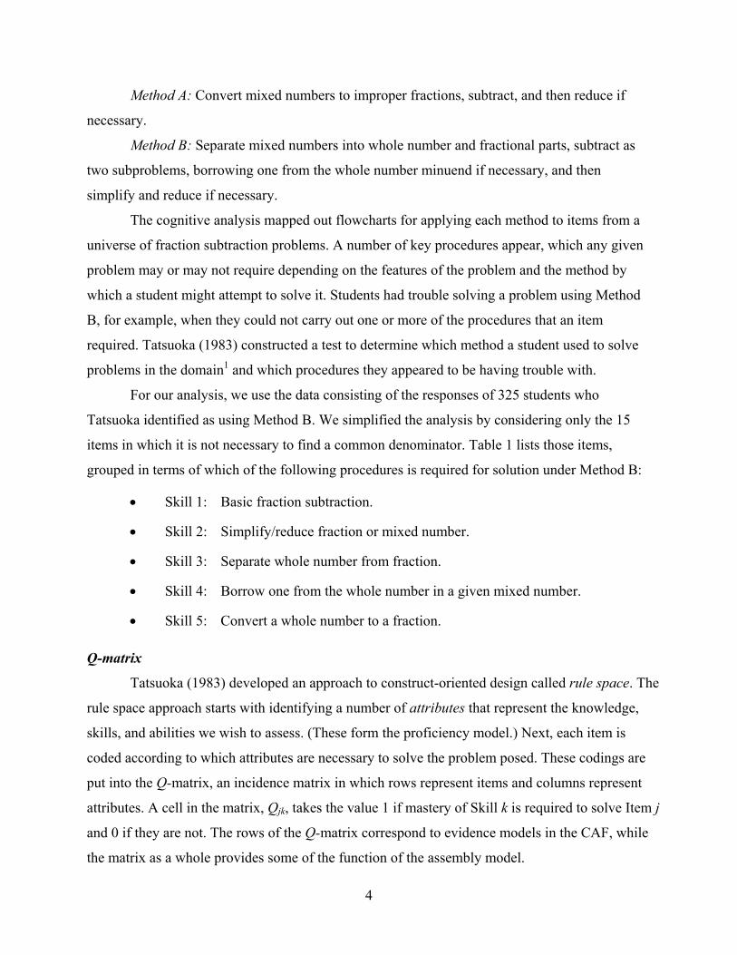
Method A: Convert mixed numbers to improper fractions, subtract, and then reduce if
necessary.
Method B: Separate mixed numbers into whole number and fractional parts, subtract as
two subproblems, borrowing one from the whole number minuend if necessary, and then
simplify and reduce if necessary.
The cognitive analysis mapped out flowcharts for applying each method to items from a
universe of fraction subtraction problems. A number of key procedures appear, which any given
problem may or may not require depending on the features of the problem and the method by
which a student might attempt to solve it. Students had trouble solving a problem using Method
B, for example, when they could not carry out one or more of the procedures that an item
required. Tatsuoka (1983) constructed a test to determine which method a student used to solve
problems in the domain1 and which procedures they appeared to be having trouble with.
For our analysis, we use the data consisting of the responses of 325 students who
Tatsuoka identified as using Method B. We simplified the analysis by considering only the 15
items in which it is not necessary to find a common denominator. Table 1 lists those items,
grouped in terms of which of the following procedures is required for solution under Method B:
• Skill 1: Basic fraction subtraction.
• Skill 2: Simplify/reduce fraction or mixed number.
• Skill 3: Separate whole number from fraction.
• Skill 4: Borrow one from the whole number in a given mixed number.
• Skill 5: Convert a whole number to a fraction.
Q-matrix
Tatsuoka (1983) developed an approach to construct-oriented design called rule space. The
rule space approach starts with identifying a number of attributes that represent the knowledge,
skills, and abilities we wish to assess. (These form the proficiency model.) Next, each item is
coded according to which attributes are necessary to solve the problem posed. These codings are
put into the Q-matrix, an incidence matrix in which rows represent items and columns represent
attributes. A cell in the matrix, Qjk, takes the value 1 if mastery of Skill k is required to solve Item j
and 0 if they are not. The rows of the Q-matrix correspond to evidence models in the CAF, while
the matrix as a whole provides some of the function of the assembly model.
4

Table 1 contains the original Q-matrix for this example. For the 15 items in this
assessment, the matrix of skill requirements for each of the items forms the Q-matrix. For
example, Items 2 and 4 require Skill 1 only; Items 1, 7, 12, 13, and 15 require Skills 1, 3, and 4
together.
Table 1
Original Q–matrix Skill Requirements for Fraction Items
Skills required Item Text 1 2 3 4 5 EM 2 6
7 − 47 = x 1
4 34 − 3
4 = x 1 8 11
8 − 18 = x x 2
9 3 45 − 3 2
5 = x x 3 11 4 5
7 −1 47 = x x 3
5 3 78 − 2 = x x 3
1 3 12 − 2 3
2 = x x x 4 7 4 1
3 − 2 43 = x x x 4
12 7 35 − 4
5 = x x x 4 15 4 1
3 − 1 53 = x x x 4
13 4 110 − 2 8
10 = x x x 4 10 2 − 1
3 = x x x x 5 3 3 − 2 1
5 = x x x x 5 14 7 − 1 4
3 = x x x x 5 6 4 4
12 − 2 712 = x x x x 6
Among these 15 items, we only see six unique patterns of skills required for the
assessment. Following the conceptual assessment framework, we call these rows evidence
models. Note that the analysis of Klein et al. (1981) called this a conjunctive model: In order to
solve a problem (e.g., Item 1) of a given type (e.g., Evidence Model 4), all of the listed skills
(Skill 1, Skill 3, and Skill 4 for Evidence Model 4) are required. The conjunctive skill model is a
purely logical one that predicts whether a student with a particular pattern of skills will be able to
answer problems from a given evidence model without making guesses or mistakes.
5
The rule space method of Tatsuoka (1983) never builds an explicit model for deviations
from the logical model. Rule space uses a pattern matching approach that containing an implicit
model for the deviations, which we will not explore here. Instead, we will explore two
approaches that take the Q-matrix and build explicit probability models for the deviations: one
based on Bayesian networks and one based on the fusion model.
Bayesian Psychometric Framework
To try and place the two different approaches within a larger context, we press into
service a general form of the psychometric models for the CAF first introduced by Almond and
Mislevy (1999). We start by defining some observable quantities:
i–student
j–task
T(i)–set of tasks “attempted” by student i
Yij–outcome (scored response) of ith student on jth task
Next, we define the proficiency model. The most important part of the proficiency model
development is identifying the variables that represent the knowledge, skills, and abilities we
wish to use in reporting. To make the model fully general (and to better illustrate the difference
between the fusion model and Bayesian networks), we divide the variables into discrete
variables, α , and continuous variables, . These variables are purely latent. They are
sometimes referred to as person parameters in the literature, but as the Bayesian framework
makes no distinction between unobserved parameters and variables, we prefer to use the term
“variable” to emphasize that they are person-specific. We reserve the term “parameter” to refer
to quantities that do not change across persons. The proficiency model is essentially the joint
distribution of the proficiency variables in the population of interest. That is,
i iθ
iα —discrete proficiency variables (latent)
iθ —continuous proficiency variables (latent)
( , | )i iP α θ λ —proficiency model: population distribution for proficiency variables
6
λ —population parameters for proficiency model
( )P λ —prior law for population parameters
The evidence models link the proficiency variables to the observable outcomes. Note that
for different rows of the Q-matrix, different patterns of skills are required. Thus the functional
form of the evidence model will vary from item to item. We group all the items that have a
common pattern of dependence on the proficiency variables and call that pattern an evidence
model. The mixed number subtraction model uses six different evidence models. While the
functional form of the distribution of the outcome variables is the same for all items within an
evidence model, the values of the individual parameters may not be.
S(j)–evidence model index (unique rows of Q-matrix)
( ) ( | , , )s j ij i i jP Y α θ π –evidence model; distribution of outcomes given proficiency
variables
jπ –item-specific evidence model parameters
( )j jP π –prior distribution of evidence model parameters
We can now assemble a general form of a predictive model for the observable
outcomes:
( )( ),
( ) ( | , , ) ( ) ( , | ) (i i i
ij s j ij i i j j j i i ij T i
P P Y dP dPλ α θ π<
= )dP∏∫ ∫ ∫Y α θ π π α θ λ λ
As the model includes prior distributions for all parameters, this is a full Bayesian model.
This has a number of important implications. First, the “scoring” process consists of applying
Bayes’ theorem to calculate the posterior distribution of the proficiency variables given the
observed outcomes. Second, even if the integrals shown above cannot be calculated analytically,
we can use MCMC to sample from posterior distributions for both proficiency variables and
parameters. Both the Bayesian network and the fusion model approach use this technique to
calibrate their models.
7

θi
λ πi
Student i
Item j
αi
Figure 2. Psychometric model for the conceptual assessment framework.
Figure 2 shows the psychometric framework as a picture using the graphical model
notation with “plates” to represent repetitions (Buntine, 1994). We notice here that proficiency
variables, α and , are replicated over persons, and the evidence model parameters, i iθ jπ , are
specific to the item. Outcomes, Yij, are replicated over both items and students, while there is
only one set of the proficiency model parameters, . λ
The following sections compare in detail the Bayesian network and fusion model in terms
of the proficiency model and evidence model.
Proficiency Model: Bayesian Network
The Mislevy (1995) model for the mixed number subtraction problem follows exactly
this framework laid out above. It starts with five proficiency variables, { 1iα ,…, 5iα },
corresponding to the five skills identified in Q–matrix in Table 1. Each of these is an indicator
variable that takes on the value 1 if the participant has mastered the skill and the value 0
otherwise. The prior (population) distribution is expressed as a discrete Bayesian
network or graphical model (Pearl, 1988). The Bayesian network uses a graph to specify the
factorization of the joint probability distribution over the skills. Note that the Bayesian network
entails certain conditional probability conditions that we can exploit when developing the Gibbs
sampler
( | )iP α λ
2 for this model. Figure 3 shows the dependence relationships among the skill parameters
provided by the expert analysis (mostly correlations, but Skill 1 is usually acquired before any of
the others so all of the remaining skills are given conditional distributions). It corresponds to the
factorization:
3 4 1 2 5 5 1 2 2 1( ) ( | ) ( | ) ( | , , ) ( | , ) ( | ) ( )WN WN WNP P P P P P P 1α α α α α α α α α α α α α α=α .
8

Prior analyses revealed that Skill 3 is a prerequisite to Skill 4. A three-level auxiliary
variable WNα (whole number skill) incorporates this constraint. Level 0 of WNα represents the
participants who have mastered neither skill; Level 1 represents participants who have mastered
Skill 3 but not Skill 4; Level 2 represents participants who mastered both skills. The relationships
between WNα , 3α , and 4α are logical rather than probabilistic; but the relationships can be
represented in probability tables with 1s and 0s.
α1
α2
α3 α4
α5
αwn
Figure 3. The graphical representation of the student model for mixed number subtraction.
The parameters of the graphical model are defined as follows: λ
1 1( 1P )λ α= =
2, 2 1( 1 |m P )mλ α α= = = for m = 0, 1
5, 5 1 2( 1 |m P )mλ α α α= = + = for m = 0, 1, 2
, , 1 2 5( |WN m n wnP n )mλ α α α α= = + + = for m = 0, 1, 2, 3
Finally, we require prior distributions, . We assume that ( )P λ 1λ , 2λ , 5λ , and WNλ are a
priori independent. (They will be a posteriori dependent because the θ variables are latent.
However, the MCMC analysis will take that dependence into account.)
The natural conjugate priors for the components of are either Beta or Dirichletλ 3
distributions. In all cases we chose the hyperparameters so that they sum to 27 (relatively strong
numbers in comparison with the sample size of 325). With such a complex latent structure,
strong priors such as the ones here are necessary to prevent problems with identifiability. These
9

must be supported by relatively expensive elicitation from the experts. Here we have given
numbers that correspond to 87% for acquiring a skill when the previous skills are mastered and
13% for acquiring the same skill when the previous skills are not mastered. They are given in the
following list:
1 (23.5,3.5)Betaλ ∼
2,0 (3.5, 23.5)Betaλ ∼
2,1 (23.5,3.5)Betaλ ∼
5,0 (3.5,23.5)Betaλ ∼
5,1 (13.5,13.5)Betaλ ∼
5,2 (23.5,3.5)Betaλ ∼
,0,* (15,7,5)WN Dirichletλ ∼
,1,* (11,9,7)WN Dirichletλ ∼
,2,* (7,9,11)WN Dirichletλ ∼
,3,* (5,7,15)WN Dirichletλ ∼
where , ,*WN mλ represents the vector of values, , ,1 , ,,...,WN m WN m nλ λ .
Proficiency Model: Fusion Model
The proficiency model takes the five discrete proficiency variables representing the skills
and adds a continuous variable, iθ , representing “other required skills not modeled in the Q-
matrix.” To avoid working with distributions that contain a mixture of discrete and continuous
variables, the fusion model uses the discrete proficiency variables α in terms of continuous i
10
proficiency variables through a Thurstonian approach of using mastery/nonmastery cut points.
For Skill k, we define a cut point, . Then we have
iα
kκ
)θα
11,...
0ik k
ikik k
k Kκκ
αα
α>
= = <
The cut points are assigned a unit normal prior distribution, (0,1)k Nκ ∼ .
We assume that the now continuous proficiency variables have a joint normal
distribution, that is, ( . To make the model identifiable, we wish to scale this
distribution to have a variance of 1 for each component; however, we wish to let the correlation
vary arbitrarily. In the fusion model, this is achieved by defining the diagonal elements of
, ) (0,i i N Σ∼
Σ to be
one and the off diagonal elements to be kmρ ∼ Unif (a, b), where 0 < a < b 1≤ . The latter restriction
prevents problems with collinearity.
We can see an immediate difference between the Bayesian network and fusion model
approaches: The Bayesian network approach uses strong prior opinion about the structure of the
proficiency variables while the fusion model attempts to be much more noninformative, using
strong priors only where necessary to keep the model away from potential problems. This latter
situation may present some problems. In particular, the prior distribution for is quite artificial,
and it is difficult to understand exactly what the region of space looks like to which it restricts
Σ
Σ .
An approach based on the Wishart distribution and the inverse of the covariance matrix (natural
conjugates) should at least be explored. The Bayesian network model, in contrast, uses natural
conjugate priors that have a natural interpretation in terms of artificial data.
Reparameterizing the fusion model to use the inverse of the covariance matrix has
another interesting consequence. The inverse of the covariance matrix can be expressed as a
graphical model similar to the Bayesian network (Whittaker, 1990); zeros in the inverse
covariance matrix express conditional independence constraints on the distribution. Thus, the
same kind of expert opinion used to build the Bayesian network proficiency model could be used
to build the fusion model.
The informative priors of the Bayesian networks do not come without a price. Generally
speaking, it takes an extensive cognitive analysis to understand the nature of the domain and the
collaboration between domain experts and psychometricians to build the proficiency model. This
11

is expensive. However, the most significant part of that expense is identifying the proficiency
variables, an expense that is shared by the fusion model.
Noisy-and Models
In the CAF, evidence models are predictive models for the outcome variables given (a
subset of) the proficiency variables. However, if we attempt to directly assess these probability
distributions for models that draw on multiple proficiency variables, we will quickly run into a
combinatorial explosion in the number of parameters we wish to assess. If the outcome variable
and all of the proficiency variables have two levels, then we need to assess 2k probabilities,
where k is the number of proficiency variables tapped for evidence mode s(j).
To reduce the number of parameters, many authors have looked at a class of models
know as noisy-or models (Pearl, 1988; Díez, 1993; Srinivas, 1993). The noisy-or type models
have readily interpretable parameters. They also separate the influences of the parent variables
allowing for factorizations of the probability distributions that can be exploited for efficient
computation. (This separable influences property is sometimes called causal independence. We
prefer the former term, which avoids using the word “causal” in a technical sense since that word
can be dissonant with its lay meaning.)
Because the models given to us by the experts are compensatory, we will build up the
noisy-and model rather than the noisy-or since the development is similar (Junker & Sijtsma,
2001). Look at a task that requires mastery of two skills for correct performance. If “Skill 1 is
mastered” and “Skill 2 is mastered,” then “Response is correct” is true; otherwise it is false. In
the engineering world, this is called an and-gate, an operator that is true if and only if all of its
inputs are true. This is expressed in the logic diagram in Figure 4.
Skill1
Skill2
Correct Response
Figure 4. Compensatory (and-gate) model.
12

Let s(j)i δ be an indicator function that is 1 if Participant I has mastered the skills required
for Item j (Evidence Model s(j) ). Then
( )
( )
1 1( 1 | , )
0 0s j
ij i js j
ifP Y
ifδδ
== = =
α π
This deterministic model is not a very realistic one in educational testing. A participant
who has not mastered one of the required skills may be able to guess the solution to a problem or
solve it via a different mechanism than the one modeled, giving a false-positive result. A
participant who has mastered all of the required skills may still fail to apply them correctly or
may make a careless error, giving a false-negative result. By providing “false-positive,” −π , and
“true-positive,” +π , probabilities, we can make a much more realistic model at the cost of only
two additional parameters.
( )
( )
1( 1 | , )
0j s j
ij i jj s j
ifP Y
ifπ δπ δ
+
−
== = =
α π
Figure 5 expresses this with a probabilistic inversion gate. Junker and Sijtsma (2001) call
this model DINA (deterministic input noisy and).
Skill1
Skill2
Correct Response
Probability of invertingoutput: False-Positive(guessing) and False-
Negative (flubbing)probabilities
Figure 5. Compensatory model with probabilitistic inversion of the outputs.
The classic approach to building a noisy-logic model is to look at inversions of the inputs.
To solve the example problem, the participant must either have mastered Skill 1 or find a way to
work around that lack of mastery. We call the probability of finding that workaround r1. If S(j)
represents the set of skills required for Evidence Model s(j), then we can express the distribution
for the outcome variable as: ( )
(1 )( 1 | , ) k
s j
ij i j jkk
P Y r α−= = ∏α π
13

Figure 6 shows this model. Junker and Sijtsma (2001) call this model NIDA (noisy input
deterministic and). Note that each of the inputs is a combination of two factors. A person can
solve the problem if the person has Skill 1 OR can find a workaround for Skill 1 AND the person
has Skill 2 OR can find a workaround for Skill 2.
Skill1
Skill2
Correct Responser1
r2
Parameters indicating thechances of solving the taskwithout having mastered the
indicated skill, that is anexception.
Figure 6. Noisy-and model with probabilistic inversion of inputs.
We can put the two different types of “noise” together to make a full noisy- and model
(Figure 7). Note that with the skill suppression parameters, jkr , the false-negative parameter
become unidentifiable (it becomes a scale factor for the jkr ’s), so we set it equal to 1. The final
probability model is then: ( )
(1 )( 1 | , ) k
s j
ij i j j jkk
P Y r απ −+= = ∏α π
Skill1
Skill2
Correct Response
Probability of invertingoutput: False-Positive
(guessing) probabilities
r1
r2
Parameters indicating thechances of solving the taskwithout having mastered the
indicated skill, that is anexception.
Figure 7. Full noisy-and model with inversion of both inputs and outputs.
14

Evidence Model: Bayesian Network
Mislevy et al. (1999) originally used the DINA model with output but not input
inversions for the evidence models for the mixed number subtraction example. Yan et al. (2003)
noted that this model caused some underfit. In particular, participants who had not mastered Skill
1 did not perform as well as predicted by the model.
To compensate, Sinharay et al. (2003) suggest “softening” the compensatory model by
separating those who had mastered no skills from those who had mastered some, but not all, of
the required skills for a particular item. However, in the Q-matrix for this assessment, the first
column (corresponding to Skill 1) is a constant vector of 1s. This means that it is impossible to
distinguish, on the basis of this test, which other skills a participant may or may not have
mastered if they have not mastered Skill 1. (This is probably not a problem operationally as the
prescription for the diagnosis “Lacks Skill 1” would almost certainly be “Review basic fraction
arithmetic operations” no matter what other skills the participant may have mastered.)
Furthermore, Skill 1 was considered a prerequisite to all of the others. As a consequence, the
new evidence model divided the participants up into three latent classes (for each type of item):
“Lacks Skill 1” (always required), “Mastered Skill 1 but lacks at least one other required skill,”
and “Mastered all required skills.” (Yan et al., 2003, used a model with only two latent classes
per item type: “Mastered the required skills” and “Lacked the required skills.”) The three latent
class (3LC) model has the following evidence model:
2 ( )
1 ( ) 1
0 1
1( 1 | , ) 0 0
0
j s j
ij i j j s j
j
ifP Y if and
if
π δπ δ απ α
== = = =
α π ≠
Finally, we must assign prior distributions for the jπ . Note that students who have yet to
master Skill 1 are probably struggling with the very basics of fraction subtraction, and it makes
sense that they would be less readily able to solve any problem. Consequently, we use a prior
distribution for 0jπ , a Beta (3.5,23.5), with a lower mean than the one we use for 1jπ , a Beta
(6,21). The prior for true positives, 2jπ , were a Beta (23.5,3.5). Note that Items 2 and 4 only
require Skill 1. Therefore, we set 0jπ = 1jπ for those items.
15

Evidence Model: Fusion Model
Both the fusion model and the noisy-and model are based on the idea that all skills for an
item are used conjunctively. Therefore, making a few substitutions in the formula for the noisy-
and model produces the fusion model. In the fusion model, the true-positive probability, πj+,
depends on the continuous proficiency variable, θi. In particular, jπ + = . This
introduces two new parameters,
* Logit( )j i ic−π θ
*jπ , which serve as “difficulty” parameters, and ci,, called the
completeness index, which measures the extent to which the item relies on the “other required
skills” variable, θi. Finally, for historical reasons, the fusion model calls the skill suppression
parameters *jkr instead of jkr . This gives the following likelihood for the fusion–model-
evidence–model: ( )
(1 )*( 1 | , ) Logit( ) k
s j
jij i j i i jkk
P Y c r απ θ −= = − ∏α π
Note that iθ enters into the equation using a Rasch-type IRT model. The role that would
be played by discrimination parameters are taken by the *jkr ’s. It is a mistake, however, to
interpret the θI as meaning the same thing as in a conventional IRT. The θI in the fusion model is
actually a residual skill and might be less confusing if it were given a different name.
All that remains is to establish prior distributions for the evidence model parameters,
. The prior distributions for * * *( , , : ( ))j j j jkc r k in S jπ π= *jπ , jc /3, and *
jkr are Beta( , )sπ πµ , c cBeta( , )sµ
and Beta( , )r rsµ . The µ ’s and s ’s are hyper-parameters. The µ ’s come from a Unif(0.1, 0.9) and
the s ’s come from a Unif(0.5, 10).
Comparison of Models
The general Bayesian psychometric framework describes a broad space of possible
models. It includes not only the models explored above, but also more conventional models such
as IRT (both unidimensional and multidimensional) and latent class models. Table 2 lists some
Bayesian psychometric models in the Bayesian psychometric framework, although this paper
only looks at the Bayesian network and fusion models.
16

Table 2
Some Bayesian Psychometric Models in the Bayesian Psychometric Framework
Model Proficiency Evidence Pros Cons
IRT Single θ Single outcome Ranking participants
Little diagnostic information
MIRT M ultiple θ; Correlational structure
S ingle outcome; Requires expert opinion
Multiple reporting scales
Expert opinion required to avoid nonidentifiability
Latent class
S ingle α; Multiple levels
Single outcome Classes can be matched to educational interventions
No details beyond class membership
Binary skills
Multiple binary α Single outcome Tied to cognitive theory of domain
Expert opinion required to avoid nonidentifiability
Bayesian network
M ultiple α; Requires expert opinion
M ultiple outcomes; Requires expert opinion
F lexible; Tied to cognitive heory of domain; t
Fast computation
Expert opinion required to avoid nonidentifiability
Fusion M ultiple binary α;
S ingle θ; Correlational structure, underlying multinormal with cut points
Single (binary) utcome; o
Expert opinion only on which proficiencies are tapped
Good measure of importance of proficiencies
Cut points can be difficult to
etermine; d Expert opinion required to avoid nonidentifiability
17

The fusion model has a very nice structure for the evidence model. In particular, the r*jk
parameters have a natural interpretation related to the importance of Skill k in solving Item j; -
log(r*) is the weight of evidence that getting Item j right provides for Skill k (L. DiBello,
personal communication, May 12, 2003). On the other hand, the proficiency model is rather
weak, particularly in the unusual choice of prior for the covariance matrix.
The Bayesian network model is very flexible, but it requires a fairly substantial input of
expert opinion to build each model. Much of the flexibility of the Bayesian network is not
explored in this paper. In particular, proficiency variables can have any number of levels, as can
observable outcome variables of items (allowing for constructed response items). Actually, some
of our work for Bayesian networks has gone further in that it uses multivariate outcomes for
complex constructed response tasks (e.g,. simulator output) that are not easily handled by other
systems (Almond et al., 2001). The theory to support these kinds of proficiency and outcome
variables has not yet been worked out for the fusion model, so we have limited our comparison
to a class of simplified Bayesian networks that are parallel with the fusion model.
In general, any Bayesian psychometric model that has a multivariate proficiency model
will require some input from experts to prevent nonidentifiability of the proficiency variables
(which could always be relabeled). This must take the form of giving some guidance as to which
items load which proficiency variables, thus making the effective definition of that variable. The
Q-matrix is a natural expression of this loading and represents the minimum required
information that must be elicited from experts to support a multidimensional model. Although
we can detect some deviations from expert-supplied Q–matrix through data analysis, we still
require that initial Q-matrix to bootstrap the process.
Note that any time there are binary (or other discrete) attributes in the proficiency model,
it will produce latent classes. These latent classes, however, more closely resemble the ones
induced by the binary skills model of Haertel and Wiley (1993). The five skills in the mixed
number subtraction model produce 32 latent classes. Including the prerequisite relationship
between Skill 3 and Skill 4 (the Bayesian network model includes this but the fusion model does
not) reduces the number of latent classes to 24.
However, not all of these 24 classes can be distinguished from the data. For example, all
tasks use Skill 1. Therefore, the 12 latent classes that lack Skill 1 are indistinguishable on the
basis of the data. Table 3 groups the latent classes into equivalence classes that can be
18

distinguished on the basis of the data. In this 15-item assessment with only six evidence models,
we can only distinguish nine different equivalence classes of proficiency variable states.
Table 3
Equivalence Classes and Evidence Models
Equivalence Evidence model Class class 1 2 3 4 5 6 description 1 No Skill 1 2 x Skill 1 only 3 x x Skill 1 & 3 4 x x x Skill 1, 3, & 4 5 x x x x Skill 1, 3, 4, & 5 6 x x Skill 1 & 2 7 x x x Skill 1, 2, & 3 8 x x x x x Skill 1, 2, 3, & 4 9 x x x x x x All skills
Note. x represents evidence models in which a student in an equivalence class is expected to make a correct response. In other words, for example, a student in Equivalent Class 8 who has Skills 1, 2, 3, and 4 is expected to make a correct response for the tasks in Evidence Models 1, 2, 3, 4, and 6.
Empirical Comparisons
Model Fitting
Procedures
The analyses for both models had the same specifications whenever possible. We used
BUGS (Spiegelhalter, Thomas, & Best, 2000; Spiegelhalter, Thomas, Best, & Gilks, 1995)and
the original Q-matrix as shown in Table 1 in the analyses for the Bayesian network. The starting
value for the parameters were from the posterior approximations in an early run (Mislevy et al.,
1999). The final model parameter estimates resulted from 2,000 iterations following 2,000 burn-
in iterations (Yan et al., 2003).
We used Arpeggio (Hartz et al., 2002) for the fusion model analyses starting with the
original Q-matrix as shown in Table 1 and following the guidelines described in Hartz et al. (2002).
We also used mild prior distributions for the hyper-parameters in the model. The results were based
on a sample of 2,000 iterations after 2,000 burn-in iterations.
19

To increase the estimation accuracy for the fusion parameters that sufficiently influence
the data as described in Skills Diagnosis: Theory and Practice (Hartz et al., 2002), the Arpeggio
estimation algorithm was expanded to sequentially drop some model parameters that appeared to
be poorly estimated or statistically insignificant based on the 95% Bayesian confidence intervals
(CI) of the posterior distribution estimates.
Our first results with the original Q-matrix and all the item and examinee parameters
showed us that many r*jk have the upper 95% CI > 0.95; 8 of the 15 ci parameters’ upper 95% CI
> 2.0; and the proportion of mastery for Skill k, , for Skill 2 and Skill 5 has quite a big 95% CI
width. For Skill 2, only two items measure the skill, which is less than the Arpeggio requirement
of at least three items in order to have a good estimate. As a result, we dropped Skill 2 due to its
lack of information in the data set. We also dropped the eight c
kP
i parameters that have big upper
95% CI in the model.
The second run resulted in another ci parameter with upper 95% CI > 2.0, so we dropped
that. The subsequent Arpeggio results turned out to have more ci parameters that have big upper
95% CI, so we proceeded to drop them one after another, and eventually we ended up dropping
all the ci parameters. We then looked at the estimates for the other parameters. There were many
r*jk that were still very big for some items ( for Skill 3 on Item 5 was 0.975, which was the
biggest), so we dropped the items. Then we found for Skill 3 on Item 9 was 0.975 and
for Skill 3 on Item 11 was 0.955, so we dropped and for Skill 3 on Items 9 and 11. As a
result, we only dropped one parameter per item each time.
*53r
*93r
*93
*11,3r
r *11,3r
After these item parameters were dropped, we found there was no r*jk > 0.95, although
for Skill 1 on Item 5 was 0.915, *51r *
10,3r for Skill 3 on Item 10 was 0.905, and many had 95% CI
width > 0.6 or 0.7 (especially for Skill 4). Now, in this model, Skill 3 and Skill 4 were completely
confounded, so both analyses with either Skill 3 or Skill 4 were the same. The final fusion model
contained Skill 1, Skill 4, and Skill 5.
Discussion
Before we begin to examine the parameters, we can already see some interesting
differences between the two approaches. In some ways, dropping the iθ parameter from the
fusion model was fortuitous, as it makes both models purely discrete and hence easier to
20

compare. In particular, we can find functions of the fusion model parameters that should be
equivalent to the Bayesian network parameters to compare them more directly.
With iθ out of the picture, the biggest difference between the fusion model and the
Bayesian network model is one of approach. The Bayesian network model is built with a fully
Bayesian approach using relatively strong priors. The fusion model takes a more data-driven
Bayesian approach using fairly weak priors. Because several skills had very few items that
tapped it, there is a fair amount of sensitivity to the choice of prior.
In particular, the test contained only two items that tapped Skill 2. The Bayesian network
model can still make inferences about that skill based mainly on the prior judgments about
relationships with other skills. The situation for Skill 3 is even stronger. Even though only three
items tapped Skill 3 without also using Skill 4, the Bayesian network model can still provide
fairly strong information about Skill 3 because of the modeled prerequisite connection between
Skill 3 and Skill 4.
Estimation Results and Comparisons
The distribution of the MCMC estimates for 1λ , the proportion of students who have Skill
1 is nicely concentrated and centered at 0.81 with a small posterior variance. 20λ is the probability
of having Skill 2 when Skill 1 is not present. This is the prior, and we learned nothing from the
data. Because of the design of the assessment, Skill 2 is present when Skill 1 is present, too. So,
21λ is the probability of having Skill 2 when Skill 1 is present; it has a tighter distribution centered
nicely at 0.92. 50λ , 51λ , and 52λ are the probabilities of having Skill 5 when having neither Skill 1
nor Skill 2, having one of them, and having both of them, respectively. They are centered at prior,
0.49, and 0.74, with 52λ having smallest posterior variance based on the data.
In the final fusion model, the ci parameters are not influential parameters and are all
dropped, so we basically do not have the iθ effects any more. Table 4 is the final Q-matrix for
the fusion model. Skill 1 is an easy skill; ’s are estimated well for the easy items, but they are
not estimated well for the hard items, with their 95% CI width > 0.4. Skill 4 is estimated well for
the hard items except for Item 3. Basically, the fusion model recognizes the easy skill, such as
Skill 1, and the hard skill, such as Skill 4 (or Skill 3). Skill 5 is not estimated well in this model,
with 95% CI width > 0.4 on all three items, which means there is not enough information for this
*r
21

parameter. The estimated has its 95% CI width = 0.2 at its borderline; it is only measured on
three items with the small data set (325 examinees), so there may not be much information for
Skill 5, either. Also, the lag 200 autocorrelation for is 0.487, which is very high, indicating the
requirement for more iterations to have good estimates for this parameter. Although the
estimates are noisy, we kept Skill 5 in the model so that we retained at least three skills. For this
assessment, Skill 3 and Skill 4 were not distinguishable. If we need to distinguish these two
skills, we will need to add more items that use Skill 3 but not Skill 4 (EM 3).
5P
5P
5P
Table 4
Final Q-matrix for Fusion Model Skill Requirements for Fraction Items
Skills required Item Text 1 2 3 4 5 EM 2 6
7 − 47 = x 1
4 34 − 3
4 =11
x 1 8 8 − 1
8 =4
x 2 9 3 5 − 3 2
5 =5
x 3 11 4 7 −1 4
7 =7
x 3 5 3 8 − 2 =
1 x 3
1 3 2 − 2 32 =
1 x x 4
7 4 3 − 2 43 =
3 x x 4
12 7 5 − 45 =
1 x x 4
15 4 3 − 1 53 =
1 x x 4
13 4 10 − 2 810 =
1 x x 4
10 2 − 3 =1
x x x 5 3 3 − 2 5 =
− 4 x x x 5
14 7 1 3 =4
x x x 5 6 4 12 − 2 7
12 = x x 6
The final fusion model is simpler than the Bayesian network model, because the final
fusion model has only Skill 1, Skill 4, and Skill 5, and it is a model based on the data set without
considering the information from the assessment designers. Our fusion model basically had two
main skills: Skill 1 for easy items and Skill 4 for hard items. By dividing the 15 items into only
easy and hard groups, we actually lost some detailed information from the assessment where
examinees mastered part of the easy items dealing with “Basic fraction subtract” (Skill 1), but
had not yet mastered “Simplifying/reducing fraction or mixed number” (Skill 2). Using the
Bayesian network, we can still make inferences about Skill 2, but they are based mainly on our
22

prior beliefs about its relationship to the other skills. This is a similar situation for Skill 5,
“Convert a whole number to a fraction.”
We now look at the proportion of masters for each of the five skills. Table 5 lists the
posterior mean for the proportion of masters for each of the five skills fit with the Bayesian
network model and each of the three skills fit with the fusion model. For comparison purposes, it
also lists the prior mean proportion of masters for the Bayesian network model.
Table 5
Estimated Proportions of Skill Masters
Skill Bayes net priors Bayes net Fusion model 1 0.870 0.803 0.711 2 0.774 0.764 ------ 3 0.815 0.824 ------ 4 0.517 0.392 0.369 5 0.739 0.600 0.354
First, Table 5 shows us the data were able to pull the Bayesian network posterior away
from the prior to a fairly large extent for Skills 1, 4, and 5 (the ones retained in the fusion
model). For Skills 2 and 3, which the fusion model drops, the Bayesian network model does not
move far from its prior at all.
Note that Skill 1 does not mean the same thing in the fusion and Bayesian network
models. Because Skills 2 and 3 were dropped in the fusion model, the new Skill 1' is the only one
required for Evidence Models 1, 2, and 3. Skill 1' incorporates some elements of Skill 2 and Skill
3 that are harder to acquire and hence rare in the population. This explains the observed
difference in Table 5.
The difference in the population proportions for Skill 5 seems quite large. This is an
artifact of the design of the test. Note that Skill 5 was only tested with Evidence Model 5, which
also includes Skill 4. Thus, it is impossible to make inferences purely from the data on the
presence of Skill 5 for persons who lack Skill 4. The Bayesian network model will assign the
presence of Skill 5 to those who lack Skill 4, with the prior probability 5 4( 1 | 0P )α α= =
approximately equal to 0.614. (This can be calculated from the mean of the prior distributions for
λ in Bayesian network software.) The observed proportion of masters for Skill 5 will be a
23
mixture of this probability for the 60% of the population who have not mastered Skill 4 and
5 4( 1 | 1P )α α= = estimated from the data for the 40% of the population who have mastered Skill 4.
P α
* *
1
K
i ikk
rπ=
∏ 0iπ
What happens in the fusion model is more complex because it depends on the correlation
between Skill 4 and Skill 5, which is difficult to estimate because of the design of the test.
However, the effect is likely to be the assumption that 5 4( 1 | 0P )α α= = is assumed to be roughly
equal to 5 4( 1 |α= = . Indeed because of the design of the assessment, we observe that the
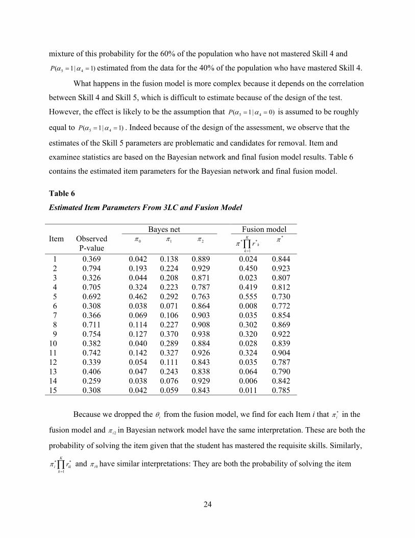
estimates of the Skill 5 parameters are problematic and candidates for removal. Item and
examinee statistics are based on the Bayesian network and final fusion model results. Table 6
contains the estimated item parameters for the Bayesian network and final fusion model.
1)
Table 6
Estimated Item Parameters From 3LC and Fusion Model
Bayes net Fusion model Item
Observed P-value
0π 1π 2π * *
1
K
kk
rπ=
∏*π
1 0.369 0.042 0.138 0.889 0.024 0.844 2 0.794 0.193 0.224 0.929 0.450 0.923 3 0.326 0.044 0.208 0.871 0.023 0.807 4 0.705 0.324 0.223 0.787 0.419 0.812 5 0.692 0.462 0.292 0.763 0.555 0.730 6 0.308 0.038 0.071 0.864 0.008 0.772 7 0.366 0.069 0.106 0.903 0.035 0.854 8 0.711 0.114 0.227 0.908 0.302 0.869 9 0.754 0.127 0.370 0.938 0.320 0.922 10 0.382 0.040 0.289 0.884 0.028 0.839 11 0.742 0.142 0.327 0.926 0.324 0.904 12 0.339 0.054 0.111 0.843 0.035 0.787 13 0.406 0.047 0.243 0.838 0.064 0.790 14 0.259 0.038 0.076 0.929 0.006 0.842 15 0.308 0.042 0.059 0.843 0.011 0.785
Because we dropped the iθ from the fusion model, we find for each Item i that *iπ in the
fusion model and 2iπ in Bayesian network model have the same interpretation. These are both the
probability of solving the item given that the student has mastered the requisite skills. Similarly,
and have similar interpretations: They are both the probability of solving the item
24

given that the student has not mastered any of the requisite skills. For example, 10π is the
probability of solving Item 1 given the student has not mastered any of the skills required for
Item 1. is the product of , the probability of solving Item 1 given the student has not
mastered any of the k skills. Thus the probability of solving Item 1 is the product of solving Item
1 given the student has mastered the skills
*1
1
K
kk
r=
∏ *1kr
*1π and *
11
K
kk
r=
∏ . Table 6 offers a comparison.
2,2π
*ik
k
π π
* *
1
K
i ikk
r=
∏ π
Even though the interpretation of the parameters is similar, we do not expect the numbers
to be the same because the population proportion of the skills (and even their interpretation in the
case of Skill 1) is different in the two models. For example, the value of *2π is approximately the
same as for Item 2 (from Evidence Model 1); however, the value of 2,0π is quite a bit smaller
than the value of . This is due to the difference in the population proportion for Skill 1. In
both cases, the predicted proportion correct is 78%.
* *2 2
1
K
kk
rπ=
∏
The largest discrepancies between *
1
K
i r=
∏ and ,0i comes for Items 2, 4, 5, 8, 9, and 11.
Note that these are all from Evidence Models 1, 2, or 3. By dropping Skill 2 and Skill 3, the
fusion model collapses those into a single evidence model. The 3LC model on the other hand,
distinguishes between students who have mastered Skill 1 but not Skill 2 (or 3) and between
those who have not yet mastered Skill 1. Thus π often falls between ,0iπ and ,1i . In some
cases it is higher than ,1iπ ; this is probably due to the same proportion-balancing problem seen
before.
For the other evidence models, the fusion model and the Bayesian network are in fairly
good agreement. In this case, both have enough parameters to model the data better.
Diagnostic Results and Comparisons
For the total 325 examinees, we first applied classification rate of 0.5 for their Skill 1,
Skill 4, and Skill 5 estimation results from both the fusion model results and the Bayesian
network. That is, for those examinees whose posterior probability for Skill k is greater or equal to
0.5, we classify them as “Having Skill k.” Table 7 lists the diagnostic results.
25

There are fairly good agreements for the examinee skills classification under the two
models, especially for Skill 4. Basically all the examinees are classified as either “Having Skill
4” or “Not having Skill 4” under the two models, except for six examinees. For Skill 1, 231
examinees are classified as “Having Skill 1” under both models, and 62 examinees are classified
as “Not having Skill 1” under both models. There is no misclassification where the fusion model
classifies examinees as “Having Skill 1” while the Bayesian network model classifies them as
“Not having Skill 1,” but there are 32 examinees whom the fusion model classifies as “Not
having Skill 1” while the Bayesian network model classifies them as “Having Skill 1.” For Skill
5 under both models, 108 and 113 examinees are classified as “Not having Skill 5” and “Having
Skill 5,” respectively, with 102 examinees in disagreement; they are classified as “Not having
Skill 5” under the fusion model while they are classified as “Having Skill 5” under the Bayesian
network model.
Table 7
Fusion Model and Bayesian Network Classifications at 0.5 level
Fusion model Bayes net No skill Have skill
Skill 1 No skill 62 32 Have skill 0 231
Skill 4
No skill 205 0 Have skill 6 114
Skill 5
No skill 108 102 Have skill 2 113
We then applied a classification rate of (0.4, 0.6) for the Skill 1, Skill 4, and Skill 5
estimation results from both models. For those examinees if their posterior probabilities for Skill
k was less than or equal to 0.4, we classified them as “Not having Skill k”, and if their posterior
26

probabilities for Skill k was greater than or equal to 0.6, we classified them as “Having Skill k”.
Table 8 lists the classification results for this case.
We then applied a classification rate of (0.4, 0.6) for the Skill 1, Skill 4, and Skill 5
estimation results from both models. For those examinees if their posterior probabilities for Skill
k was less than or equal to 0.4, we classified them as “Not having Skill k”, and if their posterior
probabilities for Skill k was greater than or equal to 0.6, we classified them as “Having Skill k”.
Table 8 lists the classification results for this case.
Table 8
Fusion Model and Bayesian Network Classifications at (0.4, 0.6) Level
Fusion model Bayes net
No skill Unknown Have skill
Skill 1
No skill 60 4 24 Unknown 0 0 6 Have skill 0 0 231
Skill 4
No skill 202 0 0 Unknown 4 1 1 Have skill 3 3 111
Skill 5
No skill 98 16 81 Unknown 3 3 19 Have skill 0 0 105
There are, again, fairly good agreements for the examinee skills classification under the
two models, especially for Skill 4. Three examinees in each of the “Not having Skill 4” and
“Having Skill 4” categories under both models were moved to “Unknown” or unclassified
categories because their posterior probabilities are around 0.5 and therefore are not classified.
There are still 24 examinees in the Skill 1 classification disagreement and 81 examinees in the
Skill 5 classification disagreement from the two models.
27

Table 9 lists typical individuals from the classification disagreement groups. The total
number of correct responses from the Skill 1 classification disagreement group of examinees is
between three and four. Examinees 249 and 256 both have typical response patterns from this
group. Examinee 249 had four correct responses for Items 2, 5, 8, and 11 and was missing Item 4
and 9 from Evidence Models 1, 2, and 3, which is a strong indication of having Skills 1 and 3,
but not Skills 4 and 5. Examinee 256 is a similar case but had Item 9 correct instead of Item 11
correct from Evidence Model 3.
For the Skill 5 classification, 98 examinees were classified as “Not having Skill 5” under
both models, and 105 examinees were classified as “Having Skill 5” under both models. There
were still 81 examinees in disagreement, and the total number of correct responses for this group
of examinees ranged from 3 to 11 out of 15 items. Examinee 195 and Examinee 197 had typical
response patterns in this group. They had correct responses for all of the items in Evidence
Models 1, 2, and 3, which indicates that they are very likely to have Skills 1, 2, and 3. In the
fusion model, we had to drop Skill 2 and Skill 3 during the model adjustment because only two
items tap Skill 2, and Skill 3 was confounded with Skill 4. The fusion model could not estimate
Skill 3 separately due to not having enough of the information that the model requires from the
data, so Skill 4 is a result of a combination of Skill 3 and Skill 4. However, the Bayesian network
model can use the relationship among the skills to estimate Skills 3, 4, and 5.
Table 9
Selected Examinee Responses
Item EM 1 EM 2 EM 3 EM 4 EM 5 EM 6 Examinee 2 4 8 5 9 11 1 7 12 13 15 3 10 14 6 Total249 1 0 1 1 0 1 0 0 0 0 0 0 0 0 0 4 256 1 0 1 1 1 0 0 0 0 0 0 0 0 0 0 4 195 1 1 1 1 1 1 0 0 1 0 0 0 0 0 0 7 197 1 1 1 1 1 1 0 0 0 0 0 0 0 0 0 6
28
Conclusion
In summary, the Bayesian network approach is a strong Bayesian approach using
informative priors. The fusion model, in contrast, is a data-driven Bayesian approach using weak
(diffuse, but not noninformative) priors. The Bayesian network model was able to retain more of
the skills identified by the cognitive experts, but only by relying on expert opinion. One’s
conclusions about which approach is better are likely to rest mostly on one’s opinion about the
strong priors; there is simply not enough data in a single example to shift that prior one way or
another.
However, the structural assumptions about the relationships among the items and
parameters are likely much stronger than the input priors for the parameters. In particular, the Q-
matrix is a critical piece insuring that what is claimed to be measured by the skills is actually
measured by those skills. Even though the fusion-model fitting procedures modifies the Q-matrix
to remove unidentified skills and unneeded attributes, it still relies very heavily on the initial Q-
matrix provided by the experts.
The Q-matrix plays a role equivalent to the design matrix in a more conventional
experiment. It determines which parameters will be estimable from data and which will simply
reproduce the prior information. Difficulties like the one with Skill 5 derive directly from the
specifications for this test as seen in the Q-matrix. In this particular problem, the short test length
produces a number of problems for estimation. Most of those can be seen by inspecting the Q-
matrix. The proper fix for many of these problems would be to increase the length of the test to
try to get new problem types that tap the skills in different combinations. DiBello, Crone,
Monfils, Narcowich, and Roussos (2002) call this “total and partial blocking.”
One useful result from our comparison of the two models was a graphic illustration of
which parts of the Bayesian network 3LC model were sensitive to the prior information. By
running two models, one with a strong prior and one with a weak, we discovered which parts of
the model changed and which stayed steady, helping us to identify which parts of the model were
not well-validated by the data. This comparison might be formalized into interesting kinds of
diagnostic procedures.
From a purely theoretical standpoint, we prefer the Bayesian network form of the
proficiency model to the fusion model form. The multivariate normal model underlying the
fusion proficiency model does not allow us to model the prerequisite dependency. To do this, we
29

would need to explore the prior distribution for ∑ used in the fusion model; a covariance
selection model (modeling ) might allow for richer kinds of expert opinion to be incorporated
into the model (Whittaker, 1990). On the other hand, the Bayesian network models can be
expensive to elicit. We have begun looking at applying the same Thurstonian cut-score trick that
we used with the fusion model to reduce the number of parameters we must elicit from a
Bayesian network model.
1−∑
For the evidence model, we prefer the fusion model parameterization. The parameters of
the fusion model have a natural interpretation in terms of the noisy-and model. In particular, the
parameter r has a direct interpretation in terms of the importance of Skill k for solving Item j.
Furthermore, thinking about the design of the test in terms of the Q-matrix has a powerful
analytical value.
*ik
Going forward, we would like to explore models that are hybrids of the two approaches.
Mixing the Bayesian network proficiency model with the fusion evidence model would produce
a very attractive class of models. It allows the use of additional expert opinion in the proficiency
model along with the fusion model statistics for item/skill correspondence. Furthermore,
approximating the iθ parameter with a discrete latent variable having five or seven levels would
give a fairly good approximation of the fusion model, but it would still support the fast
calculation algorithms of Bayesian networks (Pearl, 1988; Lauritzen & Speigelhalter, 1988). It
would give us a good starting place for exploring the universe of possible models encompassed
by the Bayesian psychometric framework.
30

References
Almond, R. G., Dibello, L., Jenkins, F., Mislevy, R. J., Senturk, D., Steinberg, L. S., & Yan, D.
(2001). Models for conditional probability tables in educational assessment. In T.
Jaakkola & T. Richardson (Eds.). Artificial Intelligence and Statistics 1999–2001 (pp.
137–143). San Francisco, CA: Morgan Kaufmann.
Almond, R. G., & Mislevy, R. J. (1999). Graphical models and computerized adaptive testing.
Applied Psychological Measurement, 23, 223-238.
Buntine, W. L. (1994). Operations for learning with graphical models. Journal of Artificial
Intelligence Research, 2, 159-225.
DiBello, L., Crone, C., Monfils, L., Narcowich, M., & Roussos, L. (2002). Student profile
scoring. Paper presented at the annual meeting of the National Council on Measurement
in Education, New Orleans.
Díez, F. J. (1993). Parameter adjustment in Bayes networks. The generalized noisy OR-gate.
Uncertainty in artificial intelligence. Proceedings of the Ninth Conference (pp. 99-105).
San Mateo, CA: Morgan Kaufmann.
Gelman, A., Carlin, J. B., Stern, H. S., & Rubin, D. B. (1995). Bayesian data analysis. London:
Chapman & Hall.
Gilks, W. R., Richardson, S., & Spiegelhalter, D. J. (1996). Markov chain Monte Carlo in
Practice. London: Chapman & Hall.
Haertel, E. H., & Wiley, D. E. (1993). Representations of ability structures: Implications for
testing. In N. Frederiksen, R. J. Mislevy, & I. I. Bejar (Eds.), Test theory for a new
generation of tests (pp. 359-384). Hillsdale, NJ: Erlbaum.
Hartz, S., Roussos, L., & Stout, W. (2002). Skill diagnosis: Theory and practice [Computer
software user manual for Arpeggio software]. Princeton, NJ: ETS.
Junker, B. W., & Sijtsma, K. (2001). Cognitive assessment models with few assumptions, and
connections with nonparametric item response theory. Applied Psychological
Measurement, 25, 258–272.
Klein, M. F., Birenbaum, M., Standiford, S. N., & Tatsuoka, K. K. (1981). Logical error analysis
and construction of tests to diagnose student “bugs” in addition and subtraction of
fractions (Research Report 81-6). Urbana, IL: University of Illinois, Computer-based
Education Research Laboratory.
31

Lauritzen, D .J., & Spiegelhalter, S. L. (1988). Fast manipulation of probabilities with local
representations—With applications to expert systems (with discussion). Journal of the
Royal Statistical Society, Series B, 50, 205–247.
Messick, S. (1992). The interplay of evidence and consequences in the validation of performance
assessments. Educational Researcher, 23(2), 13-23.
Mislevy, R. J. (1995). Probability-based inference in cognitive diagnosis. In P. Nichols, S.
Chipman, & R. Brennan (Eds.), Cognitively diagnostic assessment (pp. 43-71). Hillsdale,
NJ: Erlbaum.
Mislevy, R. J., Almond, R. G., Yan, D., & Steinberg, L. S. (1999). Bayes nets in educational
assessment: Where do the numbers come from? In K .B. Laskey & H. Prade (Eds.),
Proceedings of the Fifteenth Conference on Uncertainty in Artificial Intelligence (pp.
437-446). San Francisco: Morgan Kaufmann.
Mislevy, R. J., Steinberg, L. S., & Almond, R. G. (2003). On the structure of educational
assessments. Measurement, 1(1), 3-62
Pearl, J. (1988). Probability reasoning in intelligence systems: Networks of plausible inference.
San Mateo, CA: Morgan-Kaufmann.
Sinharay, S., Almond, R. G., & Yan, D. (2003). Model checking for models with discrete
proficiency variables in educational assessment. Manuscript submitted for publication.
Spiegelhalter, D. J., Thomas, A., & Best, N. G. (2000). WinBUGS (Version 1.3) [Computer
software user manual]. Cambridge: MRC Biostatistics Unit.
Spiegelhalter, D. J., Thomas, A., Best, N. G., & Gilks, W. R. (1995). BUGS: Bayesian inference
using Gibbs sampling (Version 0.50) [Computer software]. Cambridge: MRC
Biostatistics Unit.
Srinivas, S. (1993). A generalization of the noisy-or model. In Uncertainty in artificial
intelligence. Proceedings of the Ninth Conference (pp. 208-215). San Mateo, CA:
Morgan Kaufmann.
Tatsuoka, K. K. (1983). Rule space: An approach for dealing with misconceptions based on item
response theory. Journal of Educational Measurement, 20, 345-354.
Whittaker, J. (1990). Graphical models in applied multivariate statistics. New York: Wiley.
Yan, D., Mislevy, R. J., & Almond, R. G. (2003). Design and analysis in a cognitive assessment
(ETS RR-03-32). Princeton: NJ: ETS.
32

Notes 1Their analyses indicated their students tended to use one method consistently, even though an
adult might use whichever strategy appears easier for a given item. 2 A certain type of MCMC that provides numerical approximation of posterior probability
parameters in Bayesian estimation problems (Gelman, Carlin, Stern, & Rubin, 1995; Gilks,
Richardson, & Spiegelhalter, 1996). 3 A generalization of Beta distribution and a natural conjugate prior for categorical distributions.
If there are K categories, then the Dirichlet distribution has K parameters, kα , k = 1, .. K,
kk
α∑ is interpreted as a pseudo sample size, and each kα / jj
α∑ is the prior mean of the
probability for category k (Gelman, Carlin, Stern, & Rubin, 1995).
33