a comparison of conceptual rf system designs for the...
TRANSCRIPT
A Comparison of Conceptual RF System Designs for the
SSC Collider
Superconducting Super Collider Laboratory
SSCL-613 December 1992 Distribution Category: 400
X. Wang P. Coleman G. Schaffer


SSCL-613
A Comparison of Conceptual RF' System Designs for the SSC Collider
x. Wang, P. Coleman, and G. Schaffer
Superconduding Super Collider Laboratory* 2550 Beckleymeade A venue
Dallas, Texas 75237
December 1992
* Operated by the Universities Research Association, Inc., for the U.S. Department of Energy under Contract No. DE-AC35-89ER40486.


A Comparison of Conceptual RF System Designs for the SSC Collid4er
X. Wang, P. Coleman, and G. Schaffer
Abstract
The rf system for each Superconducting Super Collider (SSC) Collider ring is required
to provide a maximum of 20-MV peak voltage for beam acceleration and storage. Because
of the small revolution frequency and large number of bunches, it is important to have
good control on transient beam loading and coupled-bwJ.ch instabilities driven by the
cavity higher order modes. In this document, issues about rf system performance, cost,
and related longitudinal effects are studied. Transverse e£Dects will not be discussed here.
It has been realized that, independent of which rf system. is chosen for the Collider, a
transverse active damping system must be installed to address the transverse instability
problem.

CONTENTS
FIGURES .................................... . . . . . . . . . . . . . . . . . . . . . . .. Vll
TABLES ...... . . . . . . . . . . . . . . . . . . . . . . . . . . . . . . . . . . . . . . . . . . . . . . . . . . . . . . . viii
1.0 INTRODUCTION ... . . . . . . . . . . . . . . . . . . . . . . . . . . .. . . . . . . . . . . . . . . . . . . . . . . 1
2.0 RF REQUIREMENTS FOR THE COLLIDER .. . . . . . . . . . . . . . . . . . . . . . . . . . . 2
2.1 Transient Beam Loading. . . . . . . . . . . . . . . . . . . . . . . . . . . . . . . . . . . . . . . . . . . . 2
2.1.1 Periodic Transients. . . . . . . . . . . . . . . . . . . . . . . . . . . . . . . . . . . . . . . . . . . . 3
2.1.2 Non-periodic Transients. . . . . . . . . . . . . . . . . . . . . . . . . . . . . . . . . . . . . . . . 6
2.1.3 Beam Loading Effect on RF Control Loops" . . . . . . . . . . . . . . . . . . . . . . 7
2.1.4 Compensation of Transient Beam Loading. . . . . . . . . . . . . . . . . . . . . . . . 9
2.2 RF Power Requirements ..................... " . . . . . . . . . . . . . . . . . . . . .. 11
2.2.1 Steady-State Situation. . . . . . . . . . . . . . . . . . . . . . . . . . . . . . . . . . . . . . . .. 13
2.2.2 Periodic Transients . . . . . . . . . . . . . . . . . . . . . . . . . . . . . . . . . . . . . . . . . . .. 14
2.2.3 Injection Errors . . . . . . . . . . . . . . . . . . . . . . . . . . . . . . . . . . . . . . . . . . . . . .. 15
2.3 Cavity HOMs and Longitudinal Instabilities .. . . . . . . . . . . . . . . . . . . . . . . . .. 16
3.0 NORMAL CONDUCTING FIVE-CELLS .. . . . . . . . . . . . . . . . . . . . . . . . . . . . . .. 20
3.1 Power and Power Distribution. . . . . . . . . . . . . . . . . . . . . . . . . . . . . . . . . . . . . .. 21
3.2 Cavity HOMs and Coupled-Bunch Instabilities . . . . . . . . . . . . . . . . . . . . . . . .. 21
3.2.1 Instabilities Driven by HOMs ............ " . . . . . . . . . . . . . . . . . . . . .. 23
3.2.2 Instabilities Driven by 7r Mode ............ , . . . . . . . . . . . . . . . . . . . . .. 24
3.2.3 Other Fundamental Modes . . . . . . . . . . . . . . . . . . . . . . . . . . . . . . . . . . . .. 24
3.2.4 Requirements of the Feedback System . . . . . . . . . . . . . . . . . . . . . . . . . .. 24
3.3 System Reliability Considerations . . . . . . . . . . . . . . . . . . . . . . . . . . . . . . . . . . .. 25
3.4 Preliminary Cost Estimates . . . . . . . . . . . . . . . . . . . . . . . . . . . . . . . . . . . . . . . .. 25
3.4.1 General Breakdown Structure of Costs. . . . . . . . . . . . . . . . . . . . . . . . . .. 25
3.4.2 Estimated Cost for Five-Cell System . . . . . . . . . . . . . . . . . . . . . . . . . . . .. 26
3.5 Remarks about the System . . . . . . . . . . . . . . . . . . . .. . . . . . . . . . . . . . . . . . . . . .. 27
4.0 NORMAL CONDUCTING SINGLE-CELLS . . . . . . . . . . . . . . . . . . . . . . . . . . . . .. 27 4.1 Transients. . . . . . . . . . . . . . . . . . . . . . . . . . . . . . . . . . . . . . . . . . . . . . . . . . . . . . . .. 28
4.2 Power Requirements and System Layout. . . . . . . . . . . . . . . . . . . . . . . . . . . . .. 28
4.3 Cavity HOMs and Coupled-Bunch Instabilities .. " . . . . . . . . . . . . . . . . . . . . .. 29
4.4 System Reliability ............................ , .................... " 30
4.5 Preliminary Cost Estimates . . . . . . . . . . . . . . . . . . . . . . . . . . . . . . . . . . . . . . . .. 31
4.6 Remarks about the System . . . . . . . . . . . . . . . . . . . . . . . . . . . . . . . . . . . . . . . . .. 31

5.0 SUPERCONDUCTING SINGLE-CELLS. . . . . . . . . . . . . . . . . . . . . . . . . . . . . . . .. 32
5.1 Beam Loading. . . . . . . . . . . . . . . . . . . . . . . . . . . . . . . . . . . . . . . . . . . . . . . . . . . .. 33
5.2 Cavity Fundamental Mode and HOMs ................................ 33
5.3 Power and Power Distribution . . . . . . . . . . . . . . . . . . . . . . . . . . . . . . . . . . . . . .. 34
5.4 System Reliability. . . . . . . . . . . . . . . . . . . . . . . . . . . . . . . . . . . . . . . . . . . . . . . . .. 36
5.4.1 HERA System-History and Performance . . . . . . . . . . . . . . . . . . . . . . .. 36
5.4.2 LEP System-History and Performance . . . . . . . . . . . . . . . . . . . . . . . . .. 37
5.4.3 TRISTAN System-Performance . . . . . . . . . . . . . . . . . . . . . . . . . . . . . . .. 38
5.4.4 Performance Summary ...................................... '. .. 38
5.4.5 Klystron Availability . . . . . . . . . . . . . . . . . . . . . . . . . . . . . . . . . . . . . . . . .. 38
5.5 Preliminary Cost Estimates. . . . . . . . . . . . . . . . . . . . . . . . . . . . . . . . . . . . . . . .. 39
5.6 A Prospective Option. . . . . . . . . . . . . . . . . . . . . . . . . . . . . . . . . . . . . . . . . . . . . .. 39
5.7 Remarks about the System . . . . . . . . . . . . . . . . . . . . . . . . . . . . . . . . . . . . . . . . .. 40
6.0 COMPARISON OF THREE SYSTEMS .. . . . . . . . . . . . . . . . . . . . . . . . . . . . . . .. 40
6.1 System Performance. . . . . . . . . . . . . . . . . . . . . . . . . . . . . . . . . . . . . . . . . . . . . . .. 40
6.2 Estimated Total System Costs. . . . . . . . . . . . . . . . . . . . . . . . . . . . . . . . . . . . . .. 41
6.3 Other Costs. . . . . . . . . . . . . . . . . . . . . . . . . . . . . . . . . . . . . . . . . . . . . . . . . . . . . .. 41
6.4 Summary . . . . . . . . . . . . . . . . . . . . . . . . . . . . . . . . . . . . . . . . . . . . . . . . . . . . . . . .. 43
7.0 CONCLUSIONS...................................................... 43
ACKNOWLEDGEMENTS ............................................. 45
REFERENCES .... . . . . . . . . . . . . . . . . . . . . . . . . . . . . . . . . . . . . . . . . . . . . . . . . . .. 47

FIGURES
1. Equivalent RLC Circuit Representing RF Cavity Being Driven by Generator and Beam. ............................................... 2
2. Beam to Cavity Transfer Functions for Small Signals. ...................... 4 3. Phase Modulation Due to a Beam Gap. .................................. 5 4. Phase-modulated RF Waveform and Beam Bunches. ....................... 6 5. Phase Error at Injection of a New Batch. ................................. 7 6. Phase, Amplitude, and Tuning Loops Around a Cavity. .................... 8 7. Schematic of a Feedforward System (Dash Line). .......................... 9 8. Schematic of a Fast RF Feedback Loop (Dash Line) Around the Power Amplifier. 10 9. Cavity, Generator, and Circulator. ....................................... 12
10. Phasor Diagram for a Beam-loaded Cavity Coupled to a Power Generator (Below Transition). ..................................... 13
11. Compensation of Transient Beam Loading (sin cPB = 0). .................... 14 12. Correction of the Injection Error. ........................................ 16 13. Form Factors Fm(x) for Different Longitudinal Modes. ..................... 18 14. Attenuation Factor D. ................................................. 18 15. A Five-Cell Structure for the Collider. .................................... 20 16. Schematic of the APS Cavity. ........................................... 27 17. Power Distribution for Normal-Conducting Single-Cells. .................... 29 18. Geometry of the LHC Cavity. ........................................... 32 19. Layout of the Superconducting RF System. ............................... 35

TABLES
1. Primary Requirements of the Collider RF. ................................ 1 2. Optimum Coupling and Generator Power for Five-Cell Cavities. ............. 21 3. Comparison of HOM Measurement for One Five-Cell with
URMEL Calculation for Five Single-Cells. ................................ 22 4. Some Modes in a LEP Five-Cell Cavity That May Drive
Coupled-Bunch Instabilites. ............................................. 23 5. Longitudinal HOMs for one APS Cavity. ................................. 30 6. Estimated HOM Data for Collider Single-Cells. ............................ 33 7. Summary of Each RF System. .......................................... 43
1.0 INTRODUCTION
The main collider of the Superconducting Super Collid.er (SSC) consists of two rings,
both having a circumference of 87,120 m. Each Collider ring has its own rf system that
accelerates a proton beam from 2 TeV to 20 TeV (3.6 MeV jturn), maintains tight bunching
during beam storage, and compensates for energy loss due to synchrotron radiation. To
achieve the design luminosity of 1033 cm-2sec-1 , each proton beam has a dc current of
70 rnA and is grouped into 16000 bunches.
To ensure proper Collider operation, the current baseline design requires that the rf sys
tem for each ring provide a peak voltage of 20 MV. Since the High Energy Booster (HEB)
rf frequency at extraction is fixed at 60 MHz, the Collider rf frequency must be an in
teger multiple of that frequency. Various physics considerations-such as luminosity,
beam-beam effects, parasitic heating, single-bunch and multi-bunch instabilities, and in
trabeam scattering-lead to a choice of the Collider rf frequency range of 200-500 MHz.
In this range, 360-MHz and 480-MHz rf systems have been particularly considered because
352-MHz and 500-MHz sources are available on the market and can be slightly modified
for Collider use. Studies have shown that the two systems do not significantly differ in
their effects on the beam during acceleration and storage. However, beam transfer from
the HEB to the Collider is easier if the rf frequency of the Collider is closer to 60 MHz.
In the following discussions the Collider rf frequency is assumed to be 360 MHz. Some
primary requirements of the Collider rf system are listed in Table 1.
Table 1. Primary Requirements of the Collider RF.
RF frequency 360 MHz
Peak RF voltage 20 MV
Accelerating voltage per turn 3.6 MV
Voltage per turn at storage 0.12 MV
The unique characteristics of the Collider compared to other proton synchrotrons are
small beam revolution frequency, large number of bunches,and relatively high beam inten
sity. In a situation like this, transient beam loading and coupled-bunch instability driven
by the cavity higher order modes (HaMs) are the most dangerous factors in achieving the
design luminosity. Therefore, in order to define the optimum rf system for the Collider, it
is important to get good estimates of how well transient beam loading must be controlled,
the extra rf power associated with transient control, and the level to which the cavity
HaMs can be reduced. Other important issues such as the cost and reliability will also be
discussed.

Section 2 of this report reviews some theoretical aspects of beam loading and coupled
bunch instabilities. Sections 3, 4, and 5 describe the three rf systems under consideration:
the PEP-type, normal-conducting, five-cell cavity system, which represents the baseline
design; the APS-type, normal-conducting, single-cell system; and the LHC-type, super
conducting, single-cell system. Comparison results of the rfsystems are summarized in
Section 6.
2.0 RF REQUIREMENTS FOR THE COLLIDER In a synchrotron accelerator, rf cavities generate sinusoidal electric fields in the longi
tudinal direction that accelerate the beam repetitively and maintain longitudinal phase
stability. In the vicinity of the resonant frequency, a cavity can be modeled with a parallel
resistance-inductance-capacitance (RLC) circuit, shown in Figure 1. The rf power gener
ator that drives the cavity is represented by a current source I g • The amount of input
power required to generate a certain cavity voltage is related through the cavity shunt
impedance by
(1)
In this simplified circuit, the internal impedance of the rf generator is expressed as t, and f3 is termed the cavity coupling coefficient.
Cavity ---------------..,
c L
TIP-03658
Figure 1_ Equivalent RLC Circuit Representing RF Cavity Being Driven by Generator and Beam.
2.1 Transient Beam Loading Beam loading refers to the effects of beam passage in rf cavities. It can be considered
as a particular case of the problem of a beam's interaction with its environment.
The beam can drive the cavity in the same way that the rf power generator does. The
introduction of beam image current IB (the rf component of the beam current, which
equals twice the dc current in the Collider) will move both the phase and amplitude of the
gap voltage away from the original values. In a high-intensity proton collider like the SSC
2

Collider, the beam-induced voltage in the cavities cannot be neglected. In a steady-state
situation where the beam current is constant, the desired phase and amplitude of the gap
voltage are usually restored by properly detuning the cavity such that the effective load
presented by the cavity-beam to the rf power generator is resistive. l
However, the instantaneous beam current is not a constant, due to the non-uniform
structure of the beam around the ring. When the beam current suddenly changes, the
beam-induced voltage is established in a period of time much shorter than the beam
synchrotron period. It is impossible for the tuner to react to the current change and settle
to the new equilibrium during this time period. Before the tuner settles to the stationary
situation, the beam-cavity system undergoes a transient phase that may be very harmful
to the beam. The only way to eliminate or reduce the transient beam loading is to act via
the rf power generator to provide a fast control of the gap voltage. This determines the
required peak power and, therefore, the size of the rf power generator.
There are two types of transient beam loading that will be considered: periodic and non
periodic. In general, periodic transient beam loading is due to the non-uniform structure
of the beam current around the ring. It occurs during acceleration and storage, when the
existence of the abort gap and other gaps between two batches in the Collider presents
a periodic current change. Periodic transient beam loading also occurs at injection when
the ring is partially filled. Non-periodic transient beam loading occurs during the filling of
the machine, when a newly injected batch causes a sudden change in the beam current. In
fact, the two types of transient beam loading are the same in principle, and the injection
transients are always combined with the periodic transients.
2.1.1 Periodic Transients Periodic transient beam loading results in phase and amplitude modulations on the cav
ity voltage. As will be seen shortly, a consequence of the phase modulation of the rf voltage
is that the bunch spacing is no longer a constant. This m.ay cause serious problems such
as mismatch in the HEB-Collider transfer, coherent instabilities, and dilution of the beam
longitudinal emittance. Amplitude modulation of the rf voltage will be ignored, since it
can change the bunch shape only slightly and is unimportant in most cases.
Detailed discussion on transient beam loading and subsequent requirements on the rf sys
tem for a large proton collider can be found in Reference 2, and only an outline will be
given here. According to the Pederson model,3 when the cavity is driven by the rf gen
erator and beam at the same time, the phase and amplitude modulations of the cavity
voltage (av, Pv) are related to the phase and amplitude modulations of the beam (a B, P B)
through the cavity transfer function, as shown in Figure 2. The beam transfer function
3

for phase is assumed to be unity (B = 1), which corresponds to the equilibrium case; in
other words, there are no coherent oscillations of the bunches. When the cavity is properly
detuned from its resonant frequency, W r , such that the generator current is in phase with
the gap voltage, the frequency change is
1 (R) IB ~w = 2 Q WrfvCOS<PB, (2)
and the transfer coefficients can be expressed as
GB = GB = ~w b.w - (s + O")tan<pB , pp aa (s + 0")2 + ~w2 (3)
GB = _GB = b.w~wtan<pB + (s + 0") , pa ap (s + 0")2 + ~w2 (4)
where 0" /27r = Wr /47rQ is the cavity half bandwidth and s the complex variable. The abort
gap leads to an amplitude modulation of the beam current aB at the revolution frequency.
The relations between Pv and aB, and between av and aB are
Pv G~p + G~a tan<pB -b.w(s + 0")(1 + tan2 <PB) aB = 1 - Gfp - G:a tan <PB = (s + 0")2 - ~w2 tan2 <PB '
av G~a(1- G~) + G:aG~ -~wtan<pB(s + 0" + b.w tan <PB) aB = 1 - Gfp - G:a tan <PB = (s + 0")2 - b.w2 tan2 <PB
TlP"()3659
Figure 2. Beam to Cavity Transfer Functions for Small Signals.
(5)
(6)
It follows from Eq. (6) that in the case of small tan<PB, which corresponds to hadron
machines like the Collider, the amplitude modulation of the cavity voltage is unimportant
4

compared with the phase modulation. According to Eq. (5), the cavity acts like a low-pass
filter: Pv D.w 1 aB = --;;-1 + (s/(7) . (7)
Figure 3 shows the phase excursion of the cavity voltage over one revolution in the case
of single gap (abort gap) in a constant beam current. When the cavity has an extremely
small wall loss, it behaves like an integrator, and the maximum phase excursion D.tp max
can be expressed explicitly as
1 (R) wrf-D.tp max = 2" Q -yIBD.t,
where D.t is the length of the gap expressed in time.
18(t) ••
~~-------------------------, r--
~(t)
a
o
-Lt to T
to TIP-03660
Figure 3. Phase Modulation Due to a Beam Gap.
(8)
The phase-modulated rf waveform is shown in Figure 4 with the bunches at their nominal
azimuthal positions, in this case with synchronous phase (P B = 7r. It can been seen that
the bunches are no longer evenly spaced. This phase modulation of the beam current has
several consequences:
• The superposition of the wakefields induced by these unevenly spaced bunches may
drive certain couple-bunch modes to be unstable. Since the bunch spacing varies
gradually, these modes will have low coupled-bunch mode numbers.
• During injection, when the Collider ring is partially filled, the rf voltage is phase
modulated by the stored bunches. In a newly injeded batch, the equally spaced
5
bunches will not be captured into the center of the rf buckets. This so-called mis
match will result in coherent dipole oscillations and consequent dilution of the beam
longitudinal emittance.
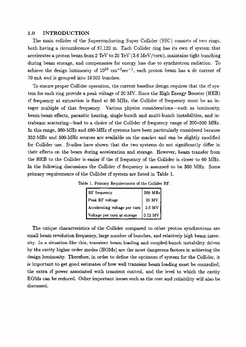
• The collision point will vary if the beams are phase-modulated, depending which parts
of the beams meet at the crossing point. Nevertheless, this effect is not important
because the bunches can be arranged such that the abort gaps of the two beams
overlap at the interaction point, so the phase variations of the two beams cancel at
that point.
1.0~~------'-Tn-------r~.------r.~~-----'~r.------'
0.5
-0.5
-- Modulated tf waveform ---- Unmodulated rf waveform
TIP-03661
Figure 4. Phase-modulated RF Waveform and Beam Bunches. (h = 5, and there are five bunches.)
It can be seen from Eq. (8) that the transient effect depends upon (~)~. This de
pendence can be understood as the following: the RIQ is inversely proportional to the
capacitance C in the equivalent RLe circuit. Therefore the amplitude of the phase modu
lation is in proportion to dv, the total charge on the capacitor. In other words, the more
energy that is stored in the cavity, the more r~sistant it is to the transients. Because a
superconducting cavity has a smaller RIQ and greater rf voltage per cavity than a normal
conducting cavity, transient beam loading will be greatly reduced when superconducting
cavities are used.
2.1.2 Non-periodic Transients Non-periodic transient beam loading typically occurs at injection, when a newly injected
batch causes the beam current to increase suddenly. When there are already stored batches
6

in the machine, this effect is always combined with the periodic transients at multiples of
the revolution frequency. In Figure 5, the phase modulation before a new batch is injected
is represented by curve a. After injection, the power source must provide extra power to
restore periodicity and bring the phase to curve b. The maximum phase error occurs when
half of the ring is filled. Its value is given as
where 6t is the length of one batch, and IB is the current of the stored beam.
Old cp(t)
/..... ____ New batch without '<::", . // , correction
/ ' / '
/ "
T 2
, , , /
'...... / , / , /
" // .....
. New batch with correction
T TIP-03662
Figure 5. Phase Error at Injection of a New Batch.
(9)
Expression (9) shows that during the filling of the ring;, the effect of the transients is
much smaller in superconducting cavities with lower R/Q and higher voltage per cavity.
2.1.3 Beam Loading Effect on RF Control Loops Another consequence of the beam loading is its effect on the rf control loops. It is a
standard technique to build independent phase and amplitude feedback loops around a.
cavity to control the rf voltage for proton machines. The resonant frequency of the cavity
is controlled by the tuning loop. Figure 6 shows a cavity (represented by a parallel RLC
circuit) with control loops around it.
When the beam current is low such that the gap volta~~e is predominantly determined
by the generator current, i.e., IIgl > IIBI, the rf control loops work satisfactorily. However,
for higher beam currents, a variation of either phase or amplitude of the beam current will
result in both phase and amplitude errors in the gap voltage. In other words, the control
loops become coupled to one another, and the beam + cavity + controls system becomes
unstable above a certain beam current threshold. For a cavity with only phase, amplitude
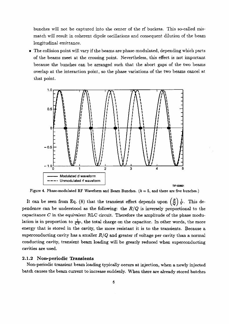
and tuning loops around it, and no acceleration (sin<pB = 0), an analytical result is given
for the beam current threshold3 as
(10)
where f p , fa, and fT are the bandwidths of the phase, amplitude, and tuning loops in the
absence of beam loading. In general, a rule of thumb that provides a reasonable safety
margin in cavity design is
where RL is the loaded cavity shunt impedance, and V is the gap voltage.
Radial position Modulator control
Frequency program
Phase loop
Amplitude loop
rf voltage control
Beam PU Beam .... rf cavity
Figure 6. Phase, Amplitude, and 'lUning Loops Around a Cavity.
rf driver
TIP-03663
(11)
For a normal conducting cavity, because of large ohmic loss on the cavity wall, the
generator current required to produce the desired gap voltage is usually greater than the
beam current. In other words, the condition (11) is easily satisfied.
In the case of a superconducting cavity, only a small amount of generator current is
needed to produce the required cavity voltage. Therefore the requirement from (11) may
determine the level to which the Q-value of the cavity must be loaded down.
8
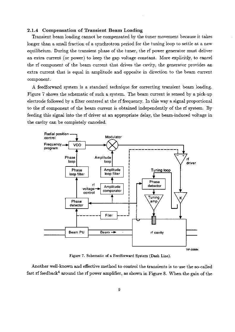
2.1.4 Compensation of Transient Beam Loading Transient beam loading cannot be compensated by the tuner movement because it takes
longer than a small fraction of a synchrotron period for the tuning loop to settle at a new
equilibrium. During the transient phase of the tuner, the rf power generator must deliver
an extra current (or power) to keep the gap voltage constant. More explicitly, to cancel
the rf component of the beam current that drives the cavity, the generator provides an
extra current that is equal in amplitude and opposite in direction to the beam current
component.
A feedforward system is a standard technique for correcting transient beam loading.
Figure 7 shows the schematic of such a system. The beam current is sensed by a pick-up
electrode followed by a filter centered at the rf frequency. In this way a signal proportional
to the rf component of the beam current is obtained independently of the rf system. By
feeding this signal into the rf driver at an appropriate delay, the beam-induced voltage in
the cavity can be completely canceled.
Radial position control
Frequency program
Phase loop
Phase loop filter
rf voltage control
Phase detector
Amplitude loop
-----_._--------,
Tuning loop
------1 Filer ~---
Beam PU Beam~ rf cavity
Figure 7. Schematic of a Feedforward System (Dash Line).
TIP·03664
Another well-known and effective method to control the transients is to use the so-called
fast rf feedback4 around the rf power amplifier, as shown in Figure 8. When the gain of the
9
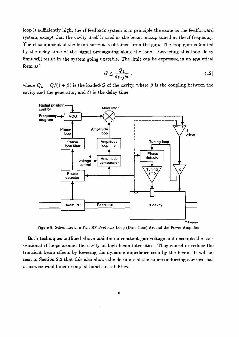
loop is sufficiently high, the rf feedback system is in principle the same as the feedforward
system, except that the cavity itself is used as the beam pickup tuned at the rf frequency.
The rf component of the beam current is obtained from the gap. The loop gain is limited
by the delay time of the signal propagating along the loop. Exceeding this loop delay
limit will result in the system going unstable. The limit can be expressed in an analytical
form asS
G< QL - 4f Tfht '
(12)
where QL = Q/(l + 13) is the loaded-Q of the cavity, where 13 is the coupling between the
cavity and the generator, and ht is the delay time.
Radial position control
Frequency program
Phase loop
Phase loop filter
rf voltage control
Phase detector
Beam PU
Modulator
Amplitude loop
Beam ....
r------------.. I r-=-1-a.""'7
I -I I I I I I I I
rf cavity
rf
TIP-03665
Figure 8. Schematic of a Fast RF Feedback Loop (Dash Line) Around the Power Amplifier.
Both techniques outlined above maintain a constant gap voltage and decouple the con
ventional rf loops around the cavity at high beam intensities. They cancel or reduce the
transient beam effects by lowering the dynamic impedance seen by the beam. It will be
seen in Section 2.3 that this also allows the detuning of the superconducting cavities that
otherwise would incur coupled-bunch instabilities.
10

2.2 RF Power Requirements In the Collider, little rf power is needed for beam acceleration because of the slow ramp
ing rate (3.6 MeV/turn), and synchrotron radiation is not as significant as in an electron
machine. However, the generator must provide enough rf power to correct transient beam
loading. Indeed the peak rf power is determined by the requirements for compensation of
the transients.
As described in Section 2.1, rf power can be saved if the cavity is properly detuned to
compensate for reactive beam loading. Furthermore, the required power can be minimized
by optimizing the coupling (;3 in Figure 1) between the generator and the cavity. Obviously
the optimum coupling depends upon the effective load presented by the cavity plus the
beam. Under different beam conditions-such as variation of the beam current, a change
from storage to acceleration mode, etc.-the total load presented by the cavity-beam sys
tem is different. Hence the optimum coupling will change accordingly.
In the case of a normal conducting cavity, the beam has relatively small influence on the
total effective load because of large power dissipation on the cavity wall. As a consequence,
the optimum coupling does not vary dramatically for different beam conditions. In the
case of a superconducting cavity, the shunt impedance of the naked cavity is so high that
the effective load is just that presented by the beam. Therefore the optimum coupling
varies greatly, depending on the beam operation conditions. When a fixed coupler is to
be used, various beam effects should be taken into account, and the coupling coefficient
should be chosen such that overall power requirements are minimized.
The beam effects to be included in rf power considerations are:
1. Injection of a new batch with a phase error;
2. Before acceleration with the ring filled and the abort gap left in the beam (peak
voltage 6.6 MV);
3. During acceleration plus the abort gap;
4. During storage at 20 TeV plus the abort gap (peak voltage 20 MV).
It will be shown that, for the CollideI', the greatest power is needed during the acceleration
process when the transients generated by the abort gap are to be corrected.
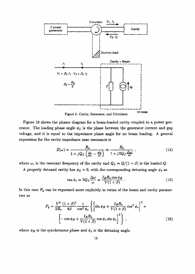
Because most of the time the load does not match the source impedance, a circulator
is always inserted between the rf power generator and the cavity to absorb the reflected
wave and protect the generator. As shown in Figure 9, the generator current Ig is equal
to twice the forward current II, and the generator power that goes into the cavity is
(13)
11
rf power generator
Zo = Rs ~
Circulator V1. 11 ~
Cavity ,. V2. 12
Cavity + Beam 1---------------1
Z
l ________ :.... _____ _
Figure 9. Cavity, Generator, and Circulator. TIP-03666
Figure 10 shows the phasor diagram for a beam-loaded cavity coupled to a power gen
erator. The loading phase angle <PL is the phase between the generator current and gap
voltage, and it is equal to the impedance phase angle for no beam loading. A general
expression for the cavity impedance near resonance is
(14)
where Wr is the resonant frequency of the cavity and QL = Q/(1 + (3) is the loaded-Q.
A properly detuned cavity has <PL = 0, with the corresponding detuning angle <Pi as
t ;/.. - 2Q ~W _ IBRscoS<PB an o/z - L W - V(l + (3) . (15)
In this case Pg can be expressed more explicitly.in terms of the beam and cavity parame
ters as
V2 (1 + (3)2 1 { [ . IBRs 2] 2 Pg = 2Rs 4(3 cos2 <Pz sm <PB + V(l + (3) cos <Pz +
IBRs . [ ]2} - cos <PB + V(l + (3) cos <Pz sm <Pz , (16)
where <P B is the synchronous phase and <Pz is the detuning angle.
12
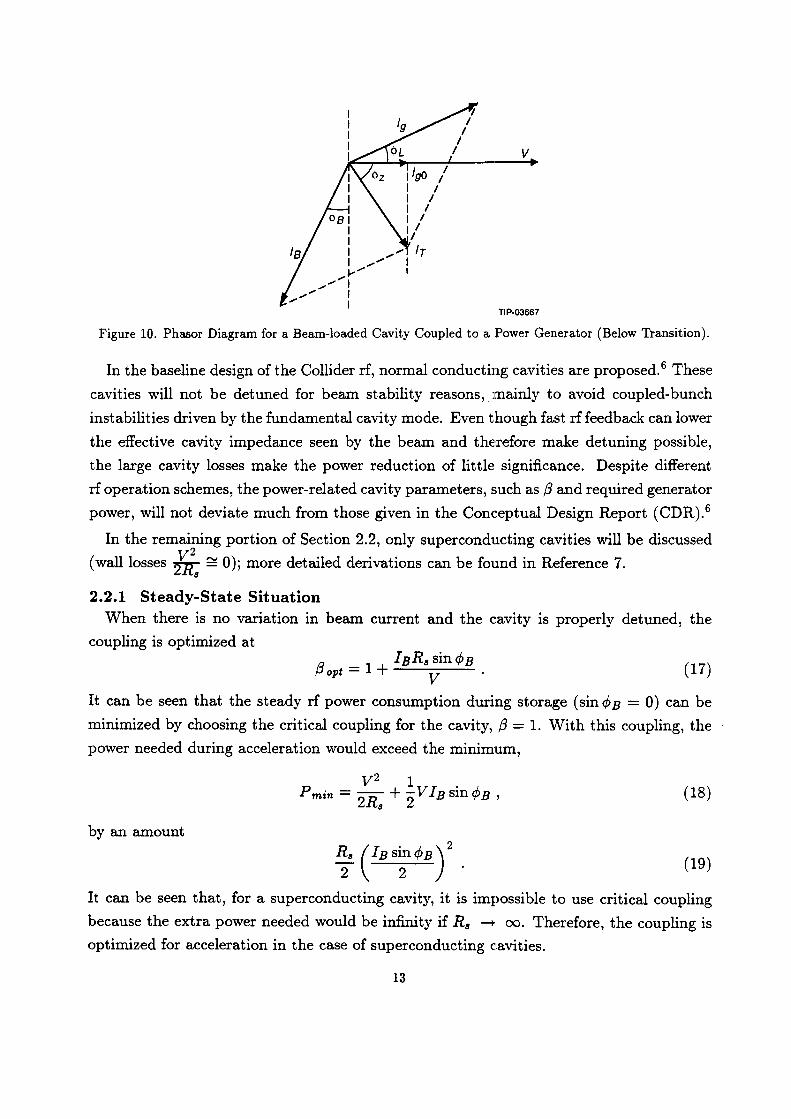
TIP-03667
Figure 10. Phasor Diagram for a Beam-loaded Cavity Coupled to a Power Generator (Below Transition).
In the baseline design of the Collider rf, normal conducting cavities are proposed.6 These
cavities will not be detuned for beam stability reasons, mainly to avoid coupled-bunch
instabilities driven by the fundamental cavity mode. Even though fast rf feedback can lower
the effective cavity impedance seen by the beam and therefore make detuning possible,
the large cavity losses make the power reduction of little significance. Despite different
rf operation schemes, the power-related cavity parameters, such as f3 and required generator
power, will not deviate much from those given in the Coneeptual Design Report (CDR).6
In the remaining portion of Section 2.2, only superconducting cavities will be discussed
(wall losses i1:s ~ 0); more detailed derivations can be found in Reference 7.
2.2.1 Steady-State Situation When there is no variation in beam current and the cavity is properly detuned, the
coupling is optimized at
(17)
It can be seen that the steady rf power consumption during storage (sin 4> B = 0) can be
minimized by choosing the critical coupling for the cavity, f3 = 1. With this coupling, the
power needed during acceleration would exceed the minimum,
(18)
by an amount
(19)
It can be seen that, for a superconducting cavity, it is impossible to use critical coupling
because the extra power needed would be infinity if Rs -+ 00. Therefore, the coupling is
optimized for acceleration in the case of superconducting cavities.
13
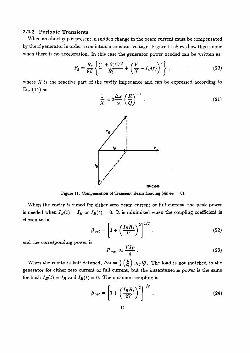
2.2.2 Periodic Transients When an abort gap is present, a sudden change in the beam current must be compensated
by the rf generator in order to maintain a constant voltage. Figure 11 shows how this is done
when there is no acceleration. In this case the generator power needed can be written as
p = Rs {(I+,8)2V2 (V -I ())2} 9 8,8 R; + X B t , (20)
where X is the reactive part of the cavity impedance and can be expressed according to
Eq. (14) as
IS /
/ /
/ /
/
/ /
/ /
/ /
v
TIP-03668
Figure 11. Compensation of Transient Beam Loading (sin tPB = 0).
(21)
When the cavity is tuned for either zero beam current or full current, the peak power
is needed when IB(t) = IB or IB(t) = O. It is minimized when the coupling coefficient is
chosen to be
[ 2]1/2
,8 opt = 1 + ( IBvRs
) ,
and the corresponding power is VIB p.",
min'" 4'
(22)
(23)
When the cavity is half-detuned, t1w = i (~) Wrf'-l. The load is not matched to the
generator for either zero current or full current, but the instantaneous power is the same
for both IB(t) = IB and IB(t) = O. The optimum coupling is
Pop, = [1+ C~:· y]'" , (24)
14
and the minimized power becomes
VIB Pmin ~ -S-· (25)
It can be seen that the required peak rf power can be reduced by a factor of two if the
cavity is half-detuned.
In fact, half-detuning the cavity during the process of acceleration can also reduce the
peak rf power.7 The optimum coupling is independent of the synchronous phase angle ¢>B
and, therefore, is the same as Eq. (24), with the corresponding rf power
P VIB ( . A.. ) min = S 2 A.. 1 + sm 'P B .
cos 'PB (26)
In the case of a fully detuned cavity with the optimized eoupling coefficient expressed in
Eq. (22), the minimum required rf power is expressed as
Pmin = V:B (1 + sin¢>B) , (27)
almost twice as much as in the half-detuning case.
2.2.3 Injection Errors A newly injected batch with current 8IB and phase error 8¢> introduces both in-phase
and quadrature errors, as shown in Figure 12. In order to correct this injection error, the
generator must provide a current I~ such that
I~2 = (Ig + 8IB sin 8¢»2 + (8IB cos 8¢»2
= I; + (8IB)2 + 2Ig8IB sin 84) ,
and from £q. (13) the corresponding power is
p . . _ R [ (V8IB)2 V8IB sin8¢>] In) - 0 1 + SPo + 41'0 '
with Po = ~k: being the rf power for no beam (matched cavity).
(2S)
(29)
In addition, it should be pointed out that the bandwidth of the cavity fundamental
mode must be large enough to handle injection errors. This can be achieved with a fast
rf feedback loop installed around the rf.
15

~~--. MBsin C\>B
8/BeGS 8C\>B
TIP-03669
Figure 12. Correction of the Injection Error.
2.3 Cavity HOMs and Longitudinal Instabilities In a high-beam-intensity accelerator, interactions of the beam with its environment
produce electromagnetic fields that drive the coherent motion of the beam bunches. The
effects of these interactions on the beam are usually described using modes of the coherent
oscillations in longitudinal phase space. The coherent motion of the particles within a
bunch is described by within-bunch modes, with mode numbers m = 1 for dipole mode,
m = 2 for the quadrupole, and so on. In addition, the coherent motions of the different
bunches may be coupled together. For M equally spaced bunches in the machine, there are
M coupled-bunch modes, each of which is designated by the couple-bunch mode index n
ranging from 0 to M -1. * The phase difference between adjacent bunches is n jT for mode n.
The spectrum associated with a coupled-bunch mode n and single-bunch mode m appears
at frequencies
fn,m = (n + pM)fo + mfs , (30)
where fo is the revolution frequency, fs is the synchrotron frequency, and -00 < p < +00
is an integer.
For the Collider, the beam parameters are chosen such that single-bunch coherent in
stabilities are not important. A major concern is the coupled-bunch instabilities due to
the large number of bunChes and small bunch spacing. When there are more than two
bunches in a machine, the upper and lower synchrotron sidebands associated with a cer
tain coupled-bunch mode belong to different revolution harmonics, except for n = 0 modes.
In other words, the synchrotron sidebands around one revolution harmonic belong to two
complementary coupled-bunch modes. Above transition, upper sidebands are unstable and
lower sidebands are stable; the opposite occurs below transition. Therefore, a narrowband
impedance object that covers both upper and lower sidebands around one revolution har
monic will always excite one coupled-bunch mode and damp its complementary mode. In
* It can run from 1 to M, depending on one's preference.
16

the Collider, obvious candidates for this type of impedance objects are the HOMs of the
rf cavities.
The mathematical model for instability treatment was originally developed by F. Sacherer
in the early 1970s.8 Interaction of a beam with its environment results in a coherent fre
quency shift. The reactive impedances of the ring contribute to the real frequency shift,
while the imaginary frequency shift or the growth (damping) rate of instabilities is de
termined by the real impedances. Assuming parabolic line density along the bunch, the
growth rate (imaginary coherent frequency shift) of an unstable coupled-bunch mode is
given by9
.6.wcm = j ( m) IB (RI~) DFm(.6.<!» , Ws m+l 3B2 hVTCOS<!>B n
(31)
where B is the bunching factor, VT is the effective rf voltage seen by the bunch, with
coherent effects such as space charge and inductive wall included, and F m is the form factor
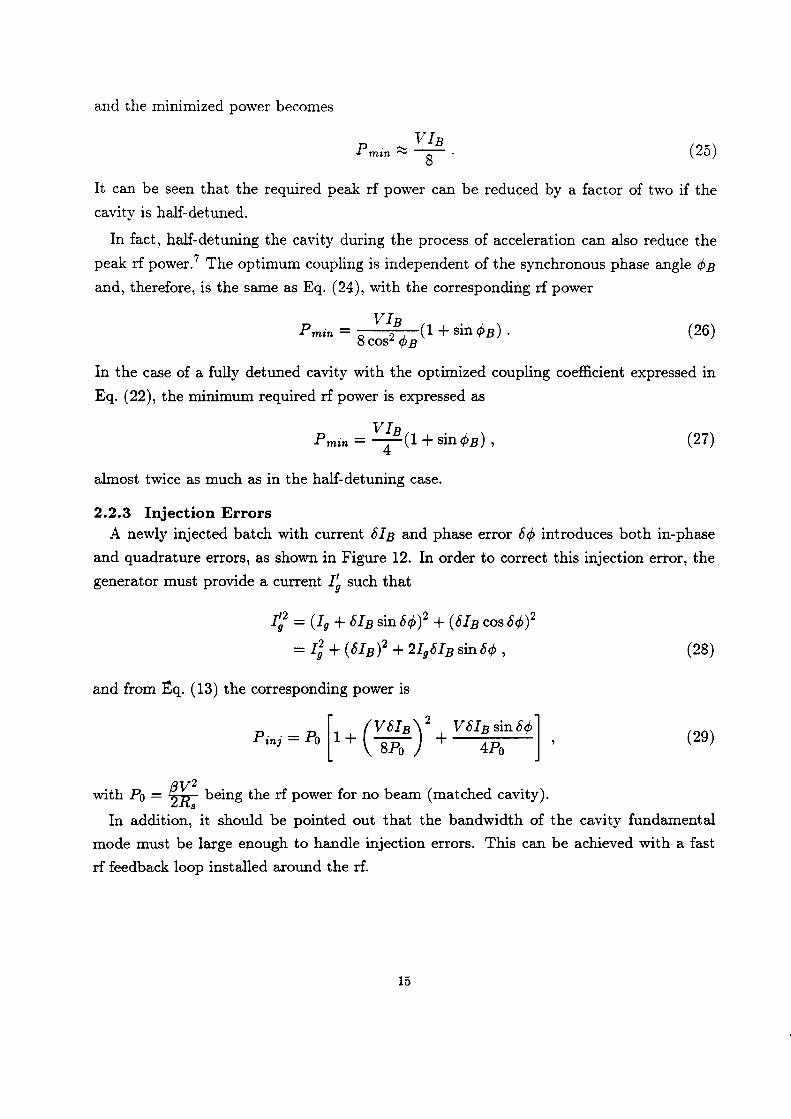
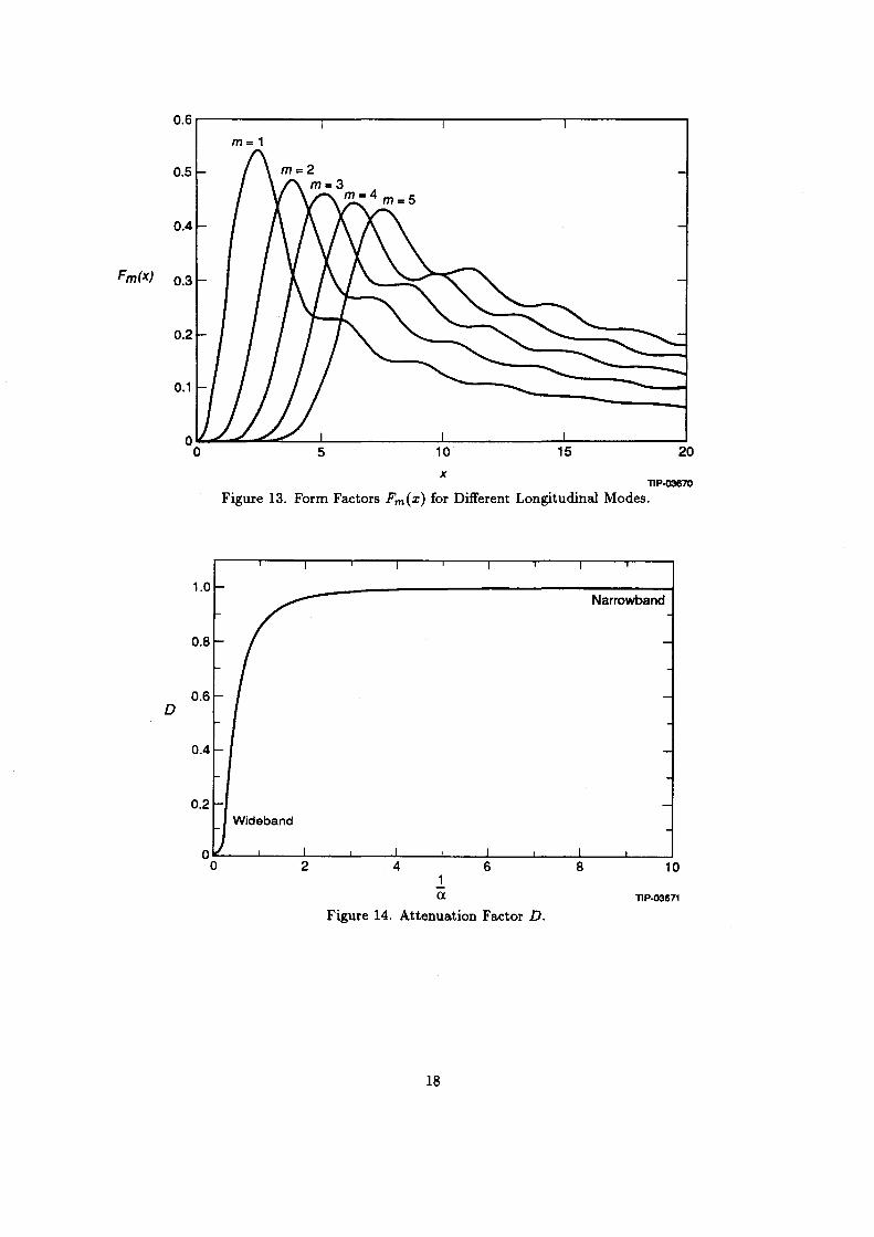
that specifies the efficiency with which the resonator can drive the mode. Figure 13 shows
the form factors for the first 5 modes. D takes into account the decay of the wakefields
between successive bunches. The coherent frequency shift is reduced by the factor D,
shown in Figure 14: a
D= , sinha
(32)
with the quantity Wr 27r 1
a = ------2QLWo M
(33)
being the attenuation between successive bunches, where Wr is the resonant frequency of
the cavity. There won't be any coupled-bunch instability if the wakefield induced by one
bunch decays appreciably before the next bunch arrives, which is the situation of low-Q
objects.
The non-linear longitudinal focusing force provided by rf field gives rise to a synchrotron
frequency spread and, potentially, to Landau damping. For small-bunch bunches, the
natural synchrotron frequency spread S is given by
1 hUJ ( )
2
S= 8" If· WsO, (34)
where Ul is the rms bunch length, h is the rf harmonic number, R is the radius of the ring,
and WsO is the synchrotron frequency for small amplitude oscillations. For the Collider
rings, Ul = 5.4 cm, R = 13,865.6 m, h = 104,544, and WsO = 47.8 sec-I. The natural
synchrotron frequency spread is
S = 0.99 sec-I. (35)
17
0.6r------------,,------------r------------~----------~
m= 1
0.5
0.4
FmM 0.3
0.2
0.1
O~'-~~~--~-----------L----------~----------~ o
1.0
0.8
0.6 D
0.4
0.2
5 10 15 20
x T1P-03670
Figure 13. Form Factors Fm(z) for Different Longitudinal Modes.
Narrowband
Wideband
2 4 6 8 10
ex T1P-03671
Figure 14. Attenuation Factor D.
18
Instabilities are Landau damped when the coherent frequency shift, including both real
and imaginary shifts, is sufficiently small compared to the natural synchrotron frequency
spread. More explicitly, calculations of the stability diagram for different particle distri
butions result in an approximate condition
(36)
where We is the coherent frequency shift.
The broadband impedance of the ring (inductive below the cut-off frequency of the beam
pipe) may cause a large enough real frequency shift of the coherent oscillation modes such
that Landau damping may be lost. In other words, ifthe real coherent frequency introduced
by reactive impedances is large enough that the mode frequency lies outside the natural
synchrotron frequency band, any small resistive impedance will cause instability. The real
frequency shift caused by the broadband impedance is expressed as
D..we 3hIB(h/M) I Z I -:;; = 27r2 B3 V cos <P B -;;: B.R'. .
(37)
For the Collider, the broadband impedance is 0.34 n (not including the broadband
impedance introduced by the liner), and the total rf voltage at injection is 6.6 MV. These
lead to a coherent frequency shift
D..we = 0.97 sec-I, (38)
which means that the broadband impedance of the Collider ring causes loss of Landau
damping.
A convenient and effective tool for coherent instability cakulations is the program ZAP.lO
For coupled-bunch instabilities, the program takes cavity and beam data as the input, and
computes the growth times of the most unstable modes. Landau-damping is also included
in the program.
It should be noticed that, in the case of the Collider, the fundamental mode of the
cavity can also drive coupled-bunch instabilities if the cavities are detuned. In the baseline
design, the normal conducting cavities have a fundamental mode bandwidth that covers
several revolution harmonics of the beam. Any detuning of the cavities will lead to unequal
resistive impedance seen by the upper and lower sidebands belonging to a certain couple
bunch mode; detuning, therefore, will drive this mode unstable. With the cavities tuned
to resonance, all the coupled-bunch modes neither grow nor damp.
However, with the fast rf feedback loop that lowers the effective shunt impedance seen
by the beam, the large bandwidth or low effective Q value results in weak couplings among
19
beam bunches. It is then possible to detune the cavity and make the growth rate small
enough that it can be easily suppressed by an active damper system. (In fact, this can be
done with the main rf system itself.)
Detuning normal conducting cavities will not save any power because of large ohmic loss
on the cavity wall and the requirements of transient corrections. On the other hand the
power needed from the generator will be greatly reduced if superconducting cavities are to
be used.
3.0 NORMAL CONDUCTING FIVE-CELLS
The baseline design for the Collider rf system consists of eight five-cell, normal
conducting cavities per ring, driven by two 1.1-MW klystrons. Details about the system
can be found in the CDR.6 For the sake of comparison with other options, a description
and preliminary cost estimates for this system will be given.
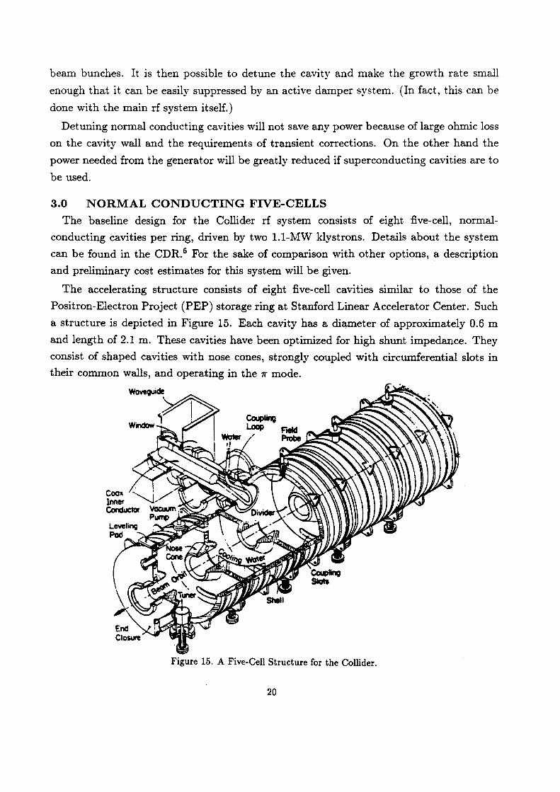
The accelerating structure consists of eight five-cell cavities similar to those of the
Positron-Electron Project (PEP) storage ring at Stanford Linear Accelerator Center. Such
a structure is depicted in Figure 15. Each cavity has a diameter of approximately 0.6 m
and length of 2.1 m. These cavities have been optimized for high shunt impedance. They
consist of shaped cavities with nose cones, strongly coupled with circumferential slots in
their common walls, and operating in the 7r mode.
Figure 15. A Five-Cell Structure for the Collider.
20

3.1 Power and Power Distribution For stability reasons, the cavities will not be detuned to compensate for reactive beam
loading. In other words, extra power from the rf power generator is the only means for
beam loading compensation. From the general expression (16) for the required rf power,
by setting the detuning angle <Pz = 0, the power from the generator is given by
(39)
Table 2 gives the optimum coupling and corresponding power for acceleration and storage
modes. In fact, for f3 values from 1 to 4 there is less than 15% change in Pg in the
acceleration phase, and only 24% in the storage mode. As discussed before, this is due to
the large wall losses of the cavity. In the baseline design, the f3 value is chosen to be 3 to
minimize the effects of beam loading. This leads to 1.74 MW power for acceleration and
1.50 MW for storage.
Table 2. Optimum Coupling and Generator Power for Five-Cell Cavities.
f3 Pg (MW)
Acceleration 1.92 1.65
Storage 1.73 1.37
The rf power is supplied by two klystron tubes, each able to deliver somewhat more than
1 MW power. This type of klystron has been produced by several European manufacturers
to support the Large Electron-Positron Collider (LEP) project at CERN. In order for one
klystron to feed four cavities, the power will be split twice with the magic-T combiners.
The reflected power of about 250 k W from each cavity will be dissipated in the dummy
load of magic-T and will not be seen by the klystron.
3.2 Cavity HOMs and Coupled-Bunch Instabilities In the CDR, calculations of the longitudinal coupled-bunch instabilities driven by the
cavity HOMs were done with ZAP. The computation was based on the cavity HOM
impedance calculated for a single-cell. There are a total of 40 cells (eight cavities) for
each Collider, so the total shunt impedance is 40 times that of a single-cell. Since all the
cavities are not identical, the frequency for each HOM varies slightly from cavity to cavity.
The calculation took this fact into account by lowering the Q values of the HOMs and
keeping the Rj Q unchanged. The de-Q-ing factor used was 20. The result showed that
the most unstable dipole mode has growth times of about 0.6 sec at injection and about
4 sec at storage.
21
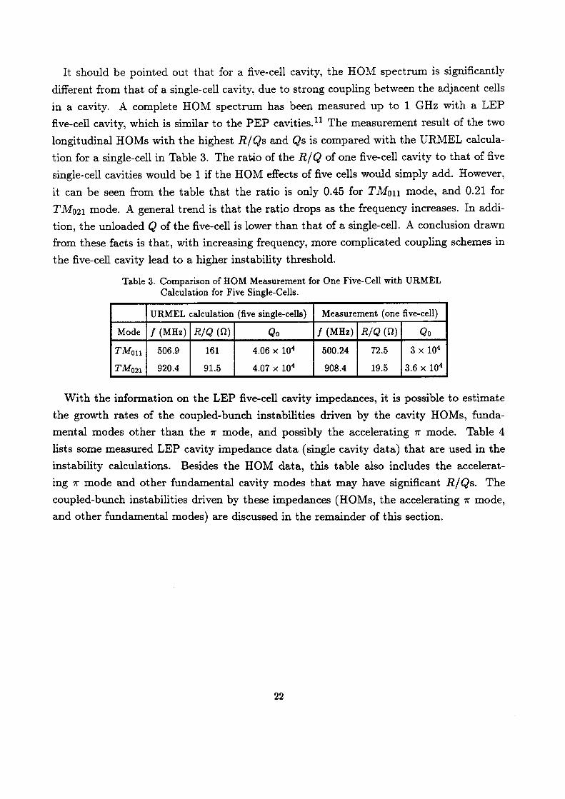
It should be pointed out that for a five-cell cavity, the HOM spectrum is significantly
different from that of a single-cell cavity, due to strong coupling between the adjacent cells
in a cavity. A complete HOM spectrum has been measured up to 1 GHz with a LEP
five-cell cavity, which is similar to the PEP cavities.ll The measurement result of the two
longitudinal HOMs with the highest R/Qs and Qs is compared with the URMEL calcula
tion for a single-cell in Table 3. The rat.io of the R/ Q of one five-cell cavity to that of five
single-cell cavities would be 1 if the HOM effects of five cells would simply add. However,
it can be seen from the table that the ratio is only 0.45 for T MOll mode, and 0.21 for
T M021 mode. A general trend is that the ratio drops as the frequency increases. In addi
tion, the unloaded Q of the five-cell is lower than that of a single-cell. A conclusion drawn
from these facts is that, with increasing frequency, more complicated coupling schemes in
the five-cell cavity lead to a higher instability threshold.
Table 3. Comparison of HOM Measurement for One Five-Cell with URMEL Calculation for Five Single-Cells.
URMEL calculation (five single-cells) Measurement (one five-cell)
Mode f (MHz) R/Q (0) Qo f (MHz) R/Q (0) Qo
™oll 506.9 161 4.06 x 10⁴ 500.24 72.5 3 x 10⁴
TMo21 920.4 91.5 4.07 x 10⁴ 908.4 19.5 3.6 x 10⁴
With the information on the LEP five-cell cavity impedances, it is possible to estimate
the growth rates of the coupled-bunch instabilities driven by the cavity HOMs, funda
mental modes other than the 7r mode, and possibly the accelerating 7r mode. Table 4
lists some measured LEP cavity impedance data (single cavity data) that are used in the
instability calculations. Besides the HOM data, this table also includes the accelerat
ing 7r mode and other fundamental cavity modes that may have significant R/ Qs. The
coupled-bunch instabilities driven by these impedances (HOMs, the accelerating 7r mode,
and other fundamental modes) are discussed in the remainder of this section.
22

Table 4. Some Modes in a LEP Five-Cell Cavity That May Drive Coupled-Bunch Instabilities.
Frequency (MHz) RIQ Qo
352.23 696 38,482
352.68 6.75 40,500
355.46 0.435 42,623
489.78 0.65 to 55 23,300
494.46 28 32,336
500.24 72.5 28,129
504.69 31.5 34,058
505.7 10.5 33,757
908.79 11.2 16,071
913.87 13.35 17,082
924.96 10 27,195
3.2.1 Instabilities Driven by HOMs ZAP has been used to calculate instability growth rates driven by vanous cavity
impedances. Very little data exists on damping of HOMs in multi-cell structures. There
fore, to obtain reasonable estimates of damped HOM levels, single-cell damping data has
been extrapolated to this multi-cell case. In particular, it is assumed two Advanced Pho
ton Source (APS)-style dampers* are installed in the cavity, one in each end-cell. The
measured performance of these dampers is then scaled by ~ in obtaining the extrapolated
loaded Qs for the five-cell HOMs. Another assumption is that the HOMs of the eight
cavities are staggered, i.e., the beam interacts only with the impedance of one cavity at a
certain HOM frequency.
If all the dangerous HOMs are effectively damped by the couplers, the most unstable
dipole mode has a growth rate of 6.6 sec. If the cavities are not stagger-tuned, the growth
time of the most unstable dipole mode becomes 0.76 sec. -
There have been concerns about the difficulty of HOM damping in the five-cell cavities
for the Collider. The rich HOM spectrum of a five-cell cavity makes it difficult to damp all
the dangerous modes without missing a single one. Some modes have field distributions
such that there are strong fields in the inner cells but no fields in the end-cells. Dampers
mounted in the end-cells would thus be ineffective. In addition, even if there are significant
fields in the end-cells, it is likely that the couplers cannot reach all the modes because of
* HOM damping result in the APS cavities is listed in Table 5, Section 4.3.
23
different field configurations of those modes. (Examples of this can be seen in the APS data
presented in Table 5, Section 4.3.) If one mode is missed in a five-cell cavity (staggered)
for example, the one with R/ Q of 21 at 506 MHz-it will drive instabilities with a growth
rate of 2 sec for the most unstable dipole mode. Missed or undamped modes may become
significant sources in driving the coupled-bunch instabilities.
3.2.2 Instabilities Driven by 7r Mode Because the bandwidth of the fundamental 7r mode of the five-cell cavity (48 kHz) is much
larger than the beam revolution frequency (3.4 kHz) in the Collider, any cavity detuning
will result in a different real impedance seen by the upper and lower sideband of the beam
current belonging to the same lower order coupled-bunch mode (e.g., n = ±1, ±2, ... ).
Therefore, it was planned not to detune the cavity for beam loading compensation. In
order to ensure that the cavity remains on resonance, information on both the phase and
the amplitude of the beam current must be included in the tuning loop. This added
complexity limits the accuracy of the tuning process. It was assumed that the loop will
maintain the detuning angle to 00 ± 10. The detuning angle ¢>z is related to a tuning error
l:!.f by l:!.f
tan ¢>z = 2QL -f . RF
(40)
A 10 error in tuning angle causes the cavity resonant frequency to be off by 300 Hz. The
most unstable dipole mode caused by the detuning has a growth rate of 2.1 sec. These
unstable modes have lower enough frequencies and can be damped through the main
rf system.
3.2.3 Other Fundamental Modes Because of the coupling between cells, the fundamental mode of the cavity splits into
a family of five modes (7r, 47r /5, 37r /5, etc.). The frequencies of the 7r mode and other
fundamental modes are quite close. Hence it would be very difficult to damp the other
fundamental modes without excessively damping the 7r mode as well. In addition, the two
fundamental modes listed in Table 4 have no fields in the middle cell on which the input
coupler is mounted. Because of these conditioI?-s, the unloaded Qs are assumed for these
two modes in the ZAP calculations. The result shows a growth rate of 1.4 sec for the most
unstable dipole mode.
3.2.4 Requirements of the Feedback System In order to address the coupled-bunch instabilities driven by the cavity impedances,
a longitudinal active damper system must be installed. The bandwidth of the damping
system is 30 MHz to cover all the possible coupled-bunch modes, and a damping rate that
24

is three to five times the growth rate of the most unstable mode would be desirable. 12 The
center frequency is assumed to be around 540 MHz, the same as in the CDR.
For a given instability damping rate, the required voltage of the feedback system can be
expressed as
(41)
where D.wd is the damping rate, and 64> is the phase errOir that the feedback detector is
able to detect.
For the five-cell system, assuming a damping rate three times the growth rate of the most
unstable mode and a phase detector resolution of 2°, the calculated rf voltage is 34 kV.
The required feedback power depends on the kicker shunt impedance. One often trades
shunt impedance of a structure for bandwidth. In this case, a 3D-MHz bandwidth is
required, and a 2-kn shunt impedance is assumed achievable. U sing a 2-kn structure
to achieve 34 kV will require 290 kW of broadband power. This represents a challenging
requirement for the source and may force the use of multiple, lower-power damper systems.
3.3 System Reliability Considerations Reliability of this rf system has been estimated in the CDR based on the PEP system
reliability. During the 1983-84 PEP run, the rf system wa.s inoperative 3.4% of the time;
during the 1984-85 run, 2.9%. Of the down time, 35% was due to low-power circuits,
which are essentially the same as the SSC Collider, and 155% was caused by high-power
circuits. Since the commissioning of the LEP, 17 1.1-MW· klystrons have been used and
have shown high reliability.
A concern about this rf system comes from the rf power distribution scheme. The
bucket-to-bunch area (95%) ratio has been chosen to be ;::: 4 to avoid excessive beam loss
due to rf phase noise. Since two klystrons are to feed eight cavities, failure of one klystron
would result in this ratio dropping to f'V 2, which would be considered unacceptable based
on Super Proton Synchrotron (SPS) experience.13
3.4 Preliminary Cost Estimates 3.4.1 General Breakdown Structure of Costs
The method of estimating the cost is the same as the standard method applied in
other projects and studies such as the Fermi National Accelerator Laboratory (FNAL)
linac upgrade and possible extension of the Los Alamos Meson Physics Facility (LAMPF)
proton linac. Available information from comparable projects at Argonne National Labo
ratory (ANL), CERN, DESY, and other laboratories has been used to obtain cost figures
as realistic as possible. Factors such as inflation and curren,cy exchange have been included
where appropriate. Details of the preliminary cost analysis can be found in Reference 14;
25

here results are summarized based on more recent information. Contingency costs are not
included in the following discussions.
The total cost of an rf system can be broken down into the following major components:
Total cost
rf equi ment { rf power .source p acceleratmg structure
personnel (engineering design & inspection, management)
buildings and utilities.
A more detailed breakdown structure of the rf equipment costs is:
Rf power source
rf power: dc power supplies, water cooling, crowbar, klystron (stand, water cooling, solenoid, filament transformer)
rf power distribution: circulator, magic-T / splitter, waveguide, dummy load, water cooling
low-level rf & rf control
Accelerating structure: cavity, input power coupler, HOM coupler, vacuum system, water distribution for a normal-conducting cavity, or cryostat, valve box and cryocontrol system for a superconducting cavity.
In this estimate, installation cost is assumed to be an additional 10% of the rf equipment
cost.
A typical breakdown of the total cost is estimated as follows: installed rf equipment,
approximately 55-60%; personnel, building, and utilities, approximately 40-45%. Because
these costs may vary significantly from one laboratory to another, they will not be discussed
here.
3.4.2 Estimated Cost for Five-Cell System For a five-cell, normal-conducting cavity system, the cost of the accelerating structure
is $0.35 million/cavity, based on the cost figure from a recent ANL purchase. The cost
for the rf power source, extrapolated from the LEP expenses, is $2.1 million/klystron per
1.1-MW unit. With a total of eight five-cell ca~ities and two klystrons for each ring, the
total cost for rf equipments is
Baseline system cost/ring = (8 x $0.35 million) + (2 x $2.1 million)
= $7.0 million.
Adding 10% for installation, the rf equipment costs $7.7 million per ring or $15.4 million
for two rings.
26

With respect to operational costs, there is a heat load of approximately 5 M~~ Iring
that must be removed from the main tunnel and klystron gallery if the normal-conducting
rf system is to be used. This cost will be compared with that for the other systems in
Section 6.
3.5 Remarks about the System Several concerns about this system are listed below.
1. Difficulty in damping the coupled-bunch instabilities driven by both the fundamental
modes and HOMs of the cavities.
2. The rf power per window is about 200 k W, which is close to the practical power limit
that a window can withstand.
3. Reliability issue: if one power source fails, the whole system goes down.
4.0 NORMAL CONDUCTING SINGLE-CELLS The second system under consideration uses 32 single-eell, normal-conducting cavities
per ring, powered by two 1.1-MW klystrons. The cavities are similar to those designed
for the APS at ANL. Figure 16 gives the cavity schematic:. The cavity shape is basically
spherical with a rounded, slightly reentrant nose cone beam pipe. This shape is optimized
for highest shunt impedance using the program URMEL. The basic cavity parameters are
R/Q = 115 n for each cavity, with an unloaded Q of 5 x 10⁴ . These are similar to the
per-cell data for five-cell cavities.
Figure 16. Schematic of the APS Cavity.
27
4.1 Transients Even though detuning the cavities is possible with fast rf feedback lowering the effective
cavity impedance to the beam, the transient must be corrected with extra rf generator
power. According to Eq. (8), when the cavities are properly detuned and there is no
compensation on the transient, the rf phase modulation of the beam is
for lllJection (42)
for storage
In the case where the cavities are not detuned, as in the baseline design, the transients are
always corrected with the generator power. Because the required rf peak power is mainly
determined by wall losses and correction of the transients, detuning the cavities will not
lower the required peak power. In other words, there is power saving with detuned cavities,
but the peak power is the same for the detuned and non-detuned systems.
To produce the required rf voltage in the Collider, the generator current for the normal
conducting cavities is larger than the beam current. Coupling among the local rf control
loops is not a problem in this case. On the other hand, the locations of the cavities and
klystrons make the loop delay too long for the fast rf feedback loop to be effective. The
transient beam-loading is to be corrected by the rf phase and amplitude control loops; if
that is not enough, a feedforward or long-delay feedback system can be used. The required
rf power will be discussed next.
4.2 Power Requirements and System Layout A primary consideration in the Collider rf system design is to use the lowest possible
number of cavities in order to reduce the total HOM impedance and to minimize the
required lattice space and system cost. However, use of a shorter accelerating structure
will result in a higher cost of the rf power system.
Generally, the rf power coupler is the most critical yet fragile component for reliable
operation of normal-conducting cavities as well as superconducting cavities. The peak
voltage for each cavity is determined by the maximum rf power that the vacuum window
of the coupler can sustain. A high power test on the APS cavity showed that the voltage
per cavity can reach 800 kV to 1 MV. For each Collider ring, 32 single-cell cavities are to be
used to produce 20-MV peak voltage, which translates to a peak voltage of 625 kV for each
cavity. This leaves a sufficient safety margin to the practical upper limit of 800 k V to 1 MV.
In addition, when considering use of the rf generator power to correct the transients, the
rf power per window should be kept below 200 kW.lS
The power required to attain the necessary peak voltage is supplied by two 1.1-MW
klystrons, as for five-cell cavities. The 32 cavities are conveniently fed by a series of
28

two-way power splitters from the klystron down to the individual cavities. The total
power requirement (1.7 MW Iring) is set primarily by cavity wall losses and transient
compensation. In other words, the required peak rf power remains the same, regardless of
the cavity detuning.
Figure 17 shows the layout of the single-cell, normal-conducting rf systems for both
Collider rings. In order to have the necessary space for cavity access, the spacing between
the cavities is 1.5 wavelengths. In addition, the input power is split once it has entered the
klystron gallery in order to make the waveguide plumbing less congested in the rf gallery of
the Collider tunnel. The total lattice space needed for the rf cavities is 40 m for one ring.
If the longitudinal active damper system is to be placed in the same region in the West
Utility section, an extra 10 m should be reserved for each ring. The total space needed for
both rings will be about 90 m. This means that the tunnel space needed for the single-cell,
normal-conducting rf system is about twice that needed for the baseline design. Taking
into account the other system components in the West Utility region-such as injection
and abort kick systems, scrapers and collimators, etc.-there is barely enough space for
the rf system.
~I 1--1.51.. TIP.Q3672
Figure 17. Power Distribution for Normal-Conducting Single-Cells.
4.3 Cavity HOMs and Coupled-Bunch Instabilities The HOMs of the APS cavities that will drive coupled-bunch instabilities have been
calculated using URMEL.16 These modes are damped by a HOM coupler mounted on
29
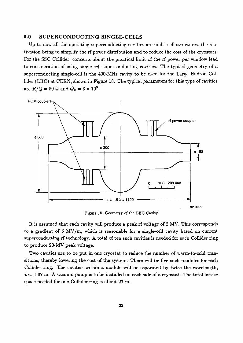
5.0 SUPERCONDUCTING SINGLE-CELLS
Up to now all the operating superconducting cavities are multi-cell structures, the mo
tivation being to simplify the rf power distribution and to reduce the cost of the cryostats.
For the SSC Collider, concerns about the practical limit of the rf power per window lead
to consideration of using single-cell superconducting cavities. The typical geometry of a
superconducting single-cell is the 400-MHz cavity to be used for the Large Hadron Col
lider (LH C) at CERN, shown in Figure 18 .. The typical parameters for this type of cavities
are RIQ = 50 n and Qo = 3 X 10⁹,
HOM couplers
1 rf power coupler
<1>680
o 100 200 mm I
L = 1.5 A = 1122
TIP·03673
Figure 18. Geometry of the LHC Cavity.
It is assumed that each cavity will produce a peak rf voltage of 2 MV. This corresponds
to a gradient of 5 MV 1m, which is reasonable for a single-cell cavity based on current
superconducting rf technology. A total of ten such cavities is needed for each Collider ring
to produce 20-MV peak voltage.
Two cavities are to be put in one cryostat to reduce the number of warm-to-cold tran
sitions, thereby lowering the cost of the system. There will be five such modules for each
Collider ring. The cavities within a module will be separated by twice the wavelength,
i.e., 1.67 m. A vacuum pump is to be installed on each side of a cryostat. The total lattice
space needed for one Collider ring is about 27 m.
32

5.1 Beam Loading Since the superconducting cavities do not have significant wall losses, the beam current
is usually greater than the generator current. In order to decouple the local rf control loops
in this high beam-loading situation, the shunt impedance, or Q, of the cavities must be
loaded down to a certain level. According to Eq. (ll), the maximum value of Q is 3 X 10⁵
for acceleration and storage, and 1 x 10⁵ at injecti~n. In fact, the cavities may be operated
at Q values higher than these as long as the fast rf feedback system is turned on to lower
the effective shunt impedance seen by the beam such that the condition given in Eq. (11)
is satisfied.
As discussed in Section 2.1.1, transient beam loading is not significant in the supercon
ducting cavities. When the cavities are properly detuned and no transient correction is
made, the maximum phase excursion for lossless cavities (the worst case) can be calculated
from Eq. (8) as for injection
(43) for storage
It can be seen that, even without any correction, the efl:ects of transient beam loading
in the superconducting cavities are about one order of magnitude smaller than those in
the normal conducting cavities, due to the high stored energy in each superconducting
cavity cell. The fast rf feedback system is needed only for decoupling the rf control loops
and eliminating the coupled-bunch instabilities driven by the fundamental mode because
of the cavity detuning.
5.2 Cavity Fundamental Mode and HOMs From Eq. (2), the necessary detuning frequency to fully compensate for reactive beam
loading is 1.9 kHz for injection and 620 Hz for acceleration/storage. In the case of half
detuning, only one half of these frequency changes are needed.
Because to this point all operating superconducting cavities have been multi-cell types,
there are no direct data on the HOMs of superconducting single-cells available. To estimate
how well the HOM couplers developed at CERN and DESy20,21 might work for the Collider
single-cell cavities, a crude scaling is made from the most updated HOM data for the multi
cell cavities at CERN and DESY.22 Table 6 gives the scaled data.
Table 6. Estimated HOM Data for Collider Single-Cells.
Mode Frequency (MHz) R/Q (0) QL
TMoll 639 55 500
TMo12 1006 22 ~11250
33

With this cavity detuning, ZAP calculations showed that the instabilities driven by the
fundamental mode have a fastest growth time of 37 sec when the gain of the fast rf feedback
system is 50. The maximum gain of the loop, given in Eq. (12), is 400 for a loop delay of
515 nsec (25 m from the beam pipe to the rf gallery x 2 plus 350 nsec delay of the klystron)
and Q L = 3 X 10⁵. This means that there is sufficient margin in the loop gain for getting a
slow enough growth rate of the coupled-bunch instabilities. In the ZAP calculation, it was
assumed that the cavity HOMs are to be staggered. If no staggered tuning is assumed,
the growth rate of the most unstable dipole mode is 5.6 sec.
5.3 Power and Power Distribution It is clear that the coupling should be optimized for the worst case, where the largest
amount of rf power is needed. For the Collider, this corresponds to the acceleration phase.
Using the formulae given in Section 2.2.2, the minimum required rf power is
{
833 kW fully detuned (Eq. (27)) with (3 = 104,
Pmin = 434 kW half-detuned (Eq. (26)) with (3 = 5000.
This translates to a minimum power of about 43.4 kW per cavity.
(44)
At injection, extra rf power needed to handle injection errors IS given by Eq. (29).
Assuming 150 injection phase error, and a newly injected batch with SIB - tIB, the
required rf power is
Pinj = 32kW , (45)
or about 3 k W per cavity.
It can be seen that the required generator power is greatly reduced compared with
the normal-conducting cavities when the superconducting cavities are half-detuned (Pg =
434 kW, or 43 kW jcell). A reasonable layout ofthe rf system is shown in Figure 19. In this
power distribution scheme, one klystron with an output power of approximately 200 kW
is used to feed two cavities. In other words, there will be five klystrons feeding ten cavities
for each Collider ring.
Compared with either normal-conducting rf system, the superconducting rf system lay
out has the following advantages:
• If one klystron or cavity fails to work,· the machine can remain operational with the
rest of the cavities on.
• When the rf power is split by the magic-Ts to feed several cavities, there is a con
cern that HOM fields may be able to propagate from one cavity to another via
* Cavity failure may be something like power-coupler discharge, but must not be a vacuum-related problem such as a broken window.
34

the magic-Ts; in other words there may be coupled-HOMs among those cavities fed
by one klystron. 23 This problem is largely reduced when a klystron feeds only two
cavities.
• Since all the cavities are not identical, transients are better controlled if one klystron
feeds fewer cavities. In the case of one klystron feeding several cavities, as in the
situation with the normal-conducting rf systems, it needs to be understood how well
a fast rf feedback system can control the cavity voltage against the transients. 24
Nonetheless, one klystron feeding two cavities is aceeptable to maintain a constant
gap voltage effectively in the case of beam loading.
• The number of cavities is not restricted to a power of 2. Choice can be based solely
on the field gradient per cavity with which one feels comfortable.
• This feeding scheme needs less waveguide plumbing, making the Collider tunnel less
congested. Of course there will be more penetrations from the rf gallery to the main
tunnel.
• When the rated power of the klystrons is about 200 k W or lower, air-insulation can
be used for the cathode instead of oil-insulation. This simplifies the klystron design,
reducing the cost.
200 kW Klystron (5 each)
180 0 3 db hybrid
(5 each)
Beam -.
-~-
TIP-03674
Figure 19. Layout of the Superconducting RF System.
Good control on beam transients can best be achieved with a power feeding scheme of
one klystron feeding each single-cell cavity. This one-on-one feeding scheme, to be used
for the LHC rf system, is motivated by beam-loading compensation.25 For the Collider,
an obvious disadvantage of this power distribution scheme is that it is expensive. It is the
desired distribution system only if the budget allows. On the other hand, the distribution
scheme shown in Figure 19 offers a good compromise between cost and cavity control.
35

5.4 System Reliability For superconducting single-cells, reliability cannot be estimated by any scaled system be
cause so far all the operating superconducting cavities are multi-cell structures. Therefore
judgement can be based only on the operational experience with the superconducting multi
cells in other laboratories. The laboratories with extensive experience in superconducting
rf systems are Continuous Electron Beam Accelerating Facility (CEBAF), 1.5 GHz; CERN
(LEP), 352 MHz; DESY (HERA), 500 MHz; and KEK (TRISTAN), 500 MHz. Among
these systems, LEP, HERA, and TRISTAN are of more interest because the rf frequencies
are close to that for the Collider.
5.4.1 HERA System-History and Performance There are three normal-conducting rf stations and one superconducting rf station in the
HERA electron ring. The superconducting cavities are four-cell structures. There are 16
such cavities powered by one klystron. These cavities are put into eight cryostats, i.e., two
cavities in one cryostat. The total rf voltage is 120 MV, one-half of which is provided by
the superconducting cavities. Donier (a German company) worked closely with DESY to
manufacture the cavities.
The reason for the mix of normal-conducting and superconducting cavities at HERA
is purely historical. When the HERA project started in 1982, only normal-conducting
cavities were proposed. Since not all the PETRA cavities were needed for the required
PETRA rf voltage, the plan was to use some PETRA cavities for HERA. The remainder
of the required HERA cavities were to be manufactured. However, during the time when
these cavities were being produced, it was found that the cavities would not be able
to meet field gradient requirements because of the lattice space limitation. In addition,
maximizing RI Q of these copper cavities would result in a dominant impedance that would
cause beam instabilities. Therefore, it was decided that superconducting cavities would be
used to finish off the HERA system, which would also allow an upgrading potential.
The HERA superconducting system had one accident in the past: a computer malfunc
tion resulted in a burst valve. Overall, operation of the superconducting rf cavities at
HERA has proven to be reliable.26 During the first run after HERA was commissioned,
the superconducting cavities were at low temperature (4.2 K) for more than 7500 hours.
The rf-on time was more than 3800 hours, and the time with beam in the machine ex
ceeded 2500 hours.26
The HERA cavities are presently run at gradients of 3.5 MV 1m '" 4 MV 1m and can be
run at 5 MV 1m. The Q-disease that the HERA cavities experienced in the past was related
to the chemical treatment of the cavities. This is well understood and can be avoided in
the future. At present, the field limitation comes from the maximum rf power that the
36

input couplers can handle. An input power of 300 kW Iwindow is considered the absolute
limit on window capability, and 100 kW Iwindow is a safe and reliable design value.
It is clear that at HERA there is no fundamental problem for the superconducting
rf cavities and superconducting magnets to share one cryogenic system (both at 4.2 K).
Superconducting cavities and magnets demand different liquid helium pressure, which can
be assured easily by an additional valve box for each cryostat. Having one cryosystem
for both the cavities and magnets has the advantage of lower cost, although it introduces
some inconvenience. In the case of HERA, when the magnets warm up, the cavities must
do so as well. In addition, more valve boxes are needed to protect the cavity system,
adding some complexity to the design. However, experts at both DESY and CERN have
suggested that the SSC Collider consider having the cavities and magnets share the same
cryosystem if superconducting cavities are to be used.
5.4.2 LEP System-History and Performance There are 128 five-cell, normal-conducting cavities at LEP that provide a total peak
voltage of 400 MV. The cavities are powered by 16 1.1-MW klystrons. There are also
12 four-cell, superconducting cavities in the machine. Niobium-coated copper cavities are
used for LEP instead of pure niobium cavities because of lower cost and better perfor
mance. Currently the LEP superconducting cavities are running at an average gradient of
approximately 4 MV 1m with beams in the machine. In LEP Phase 11,192 superconducting
cavities will be installed in addition to the existing normal conducting cavities, providing
enough power for beams at the top energy of 90 Ge V.
There were two problems with the superconducting cavities at the beginning of the first
LEP run in 1990. One was the helium bath pressure oscillations that caused corresponding
changes of the resonant frequency. The tuning loop was unable to react quickly enough, re
sulting in a sharp drop in the cavity voltage, which in turn caused a false quench detection.
The reason was soon understood; transition from room temperature to low temperature
was· made smooth for the liquid helium cooling line, and the problem disappeared. The
other problem involved excessive heating of some HOM couplers. Because of the orienta
tion of the helium cooling lines for those couplers, they picked up gas helium instead of
liquid helium from the transfer line when it contained two-phase helium in it. At the same
time the other couplers worked well. The cooling line has been modified slightly to solve
the problem.
The LEP cavities have been working reliably since these problems were understood and
solved. It has been realized that the reliability problems of the rf system, either normal
conducting or superconducting, are not usually associated with the cavities themselves;
37

rather, they are correlated with operation at high power levels. Problems such as window
failures, overheating of the waste loads, etc., occur when the system is running at high
power.
Recently, some LEP cavities experienced a problem with input power couplers. Arcing in
that region resulted in metalized windows. The reason was said to be that the windows had
been conditioned only with traveling waves, not with standing waves.27 This indicates that
superconducting cavities must be treated with extreme care. In order to avoid repeating
these types of problems at the SSCL, one obviously would want to take advantage as much
as possible of the operational experience with existing superconducting systems.
5.4.3 TRISTAN System-Performance TRISTAN has 32 five-cell superconducting cavities operated at 500 MHz. The cavities
are able to run at 5 MV 1m (currently run at 3-4 MV 1m) with the beam in the machine,
and they produce a total voltage of 140 MV. Since commissioning in late 1988, the accu
mulated time for these cavities at low temperature (4.4 K) has been 16,000 hours, and the
accumulated time for physics experiments has been more than 8300 hours.
In general these superconducting cavities have been reliable. Synchrotron radiation of
the electron beam did cause trips of the cavities near the arc sections of the machine. By
adjusting the mask positions, the rate at which cavities tripped has been substantially
reduced.
5.4.4 Performance Summary Operating experience with superconducting cavities at different laboratories has proven
that superconducting rf technology has matured to the point that it is as reliable as a
normal-conducting rf system. This high reliability is achieved when the system is not
pushed to its high power extreme.
The reason that TRISTAN, HERA, and LEP all have a mixture of normal-conducting
and superconducting cavities is purely historical: decisions had to be made before people
had enough confidence about superconducting rf technology.
5.4.5 Klystron Availability Because design of a new klystron product Incurs additional R&D cost and gener
ally requires two to three years of work, use of existing tubes is preferred. At present,
the klystrons in the 360-MHz frequency range are the 1.1-MW tubes at LEP and the
600-kW tubes at PEP. Philips personnel have said they could modify their 352-MHz LEP
klystron design for the 360-MHz SSC Collider system and deliver a tube in approximately
nine months. At the 200-kW level, Thomson-CSF personnel say they are developing a
38
368-MHz tube for the DA0NE experiment in Frascati, Italy, that could be easily modified
for the 360-MHz SSC Collider system.
5.5 Preliminary Cost Estimates For each superconducting single-cell, the cavity cost-induding cavity, input power cou-
pler, HOM coupler, cryostat, instrumentation, and cavity control-is $0.375 million/cavity;
a valve box costs about $0.15 million, so the total cost for ten cavities is
total cavity cost = (10 x $0.375 million) + (5 x $0.15 million)
= $4.5 million.
Here it is assumed that the rf system will share the cryogenic system with the supercon
ducting magnets. The advantage is cost reduction: only a valve box rather than a cryoplant
is needed for each cryostat. The disadvantage is that cold operation of the rf system may
be subject to cryoplant downtime imposed by the magnets.
Budgetary quotes are presently being prepared by Thomson-CSF on its 200-kW klystron.
In lieu of that quote, the rf power source cost is estimated using an approximate rule of
thumb: the cost is proportional to the square root of the rf power. For a 200-kW power
source, the estimated rfpower cost is $4.5 million (based on $2.1 million per 1.1-MW power
system cost). A 10% installation cost should be added as for the other systems, resulting
in the total rf system cost (rf power and accelerating strueture) of $9.9 million/ring.
In addition to the initial capital investment for the rf system itself, the heat load that
must be removed from the rf system (klystrons and dummy loads) during Collider op
erations is estimated to be 2.5 MW Iring, compared with 5 MW Iring for the normal
conducting systems. The impact of each system on future operations will be discussed in
Section 6.
5.6 A Prospective Option Consideration has been given to the use of eight superconducting single-cell cavities,
instead of ten, to provide 20-MV peak rf voltage for each Collider ring. Each cavity will
produce 2.5 MV voltage, which is translated to a gradient of 6 MV /m. This gradient is
considered slightly too high for a conservative conceptual design at this time. However,
based on the current trend of the accelerating field gradient of the superconducting cavities,
this layout may become attractive in terms of both cost and performance.
At present, the operating multi-cell superconducting cavi.ties are routinely run at average
field gradients of 3.5-5 MV /m. Since each single-cell cavity can be optimized individually,
the field gradient can be higher than the average value for a multi-cell cavity. In addition,
research on achieving much higher field gradient in the future appears promising. The
39

multi-cell niobium-sputtered copper cavities developed at CERN have led to a 30% increase
in gradient. In the rf test laboratories, gradients of 15-20 MV 1m have been achieved. These
results show a good prospect for reaching significantly higher gradients than 5 MV I m in
the presence of beam.
In the case of eight single-cell superconducting cavities per ring, it is possible to use one
small klystron to feed each cavity without escalating the cost. Cost can be further reduced
if one klystron feeds two cavities.
5.7 Remarks about the System The advantages of superconducting rf cavities have become well known. In general,
they require less lattice space, are capable of higher rf voltage per cell, have fewer HOMs,
and have lower rf power requirements. With superconducting cavities, gap transients and
coherent beam instabilities are greatly reduced.
A difficulty associated with this system is that superconducting rf technology is more
complicated than that for the other two systems. Various issues must be dealt with, includ
ing sensitivity to contamination, increased assembly complexity, vibration sensitivity, extra
controls, and the extra lab infrastructure required to support the use of superconducting
cavities. Expertise on superconducting rf must be developed at the SSCL in the process
of the rf system construction. This can be achieved with help from other laboratories.
6.0 COMPARISON OF THREE SYSTEMS
Sections 3, 4, and 5 have described in detail three designs for the Collider rf system
based on eight five-cell, normal-conducting cavities, 32 single-cell, normal-conducting cav
ities, and ten single-cell, superconducting cavities, respectively. Comparison among these
three systems will be based on system performance, required tunnel space in the Collider
West Utility region, estimated total cost of the system, impact of each system on tunnel
construction, and future Collider operations.
6.1 System Performance A major concern in the drive to achieve the design luminosity is the coupled-bunch
instabilities driven by the HOMs of the rf syst~m. Both single-cell systems have advan
tages over the five-cell system in this aspect, since HOM damping for single-cells is much
more effective. Moreover, the superconducting cavities have fewer HOMs. These modes
can be sufficiently damped using CERN-designed HOM couplers. This eases the power
requirement in the longitudinal active damper design.
The input rf power needed for the superconducting single-cell system is substantially less
than the power needed for the normal-conducting systems. For superconducting cavities
the minimum required rf power is 0.43 MW, compared with more than 1.7 MW for the
40
normal-conducting cavities. The difference is due to the small wall losses of the supercon
ducting cavities.
Operating with a smaller number of cavities-eight to ten-has the obvious advantage
of simpler waveguide plumbing schemes. Fewer cavities also allow consideration of using
one klystron per cavity. Ideally, driving each cavity with :its own klystron would provide
the maximum control of the gap voltage and would make rf feedback easier to implement.
This also would mean if one klystron-cavity system were to go down, Collider operations
could continue. Besides, the klystron design will be simpler and more reliable because of
the air-insulation for the cathode instead of oil-insulation. However, the overall system
cost escalates significantly as the number of klystrons increases. The proposed one klystron
per two cavities for the superconducting system is seen as a reasonable compromise. A
similar strategy could be adopted for the five-cell, normal-conducting system; however, the
cost would be greater than what has been discussed in this report.
6.2 Estimated Total System Costs The normal conducting single-cell system is the most expensive of the systems consid-
ered. If two 1.1-MW klystrons are used, the total capitall investment for the single-cell,
normal-conducting rf system is about $12.1 million/ring, which represents a 60% increase
in cost from the baseline five-cell cavity system. The superconducting rf system costs
$10.7 million/ring, slightly lower than the single-cell, normal-conducting rf system. How
ever, this estimate is rough because of the lack of a klystron quotation.
6.3 Other Costs Active longitudinal damping systems have not been addressed in detail in this report.
However, it should be noted that the poorer the performance of the main accelerating
system with respect to driving instabilities, the more powerful the active damper must be.
High-power, wideband rf amplifiers in the 600-800 MHz frequency range will be difficult
to find and will probably be expensive.
In terms of conventional construction, because the 32-single-cell, normal-conducting
rf system occupies about twice as long a lattice space as the other two systems, there is
extra cost for the tunnel space needed for this system in the rf gallery. A rough estimate of
$200/yd3 for tunneling leads to an additional cost of $0.5 million for the normal-conducting,
single-cell system.28
Cooling plant costs scale directly with the rf power. Assuming a ",50% klystron effi
ciency, the utility power requirements are ",5 MW Iring for a normal-conducting system
and ",2 MW Iring for the superconducting system. Less than half of this power is delivered
to the cavities, with the remainder being dissipated in the klystrons and other components
41

in the system. For a lOoC temperature rise, the normal-conducting system would require
"" 2250 gallons per minute (GPM)/ring. At $1000/GPM,29 the cost for the cooling plant
would be $2.25 million/ring. On the other hand, the cooling plant for the superconducting
rf system would cost", $0.9 million/ring.
A cost item that is unique to the superconducting system is the cryoplant. For a cryo
plant capacity of 500 W, the cost is estimated to be $0.5-0.8 million.
During Collider operations, the water cooling system will have to remove about 5 MW of
power per ring from the tunnel and klystron gallery when the normal-conducting rf system
is used. This requires a pumping system of roughly 325 hp for each ring, 30 whereas for
the superconducting cavities, only one-third of this power needs to be removed. The
electricity cost is proportional to the amount of power that needs to be taken out of
the tunnel. Assuming a machine operating time of 67% each year and a cost of 5 cents
per kWh, the annual cost of electricity for removing the heat load from the Collider
tunnel is approximately $140,000 for the normal-conducting rf system and $30,000 for the
superconducting system. In addition, the deionization bottles need to be replaced roughly
once every other month. For a cooling system that has more water flow, there are more
such bottles, and the replacement cost is higher. But it would be unrealistic to estimate
the cost at this time.
Another factor that will influence Collider operational cost is the required utility power.
With the same assumptions of 5 cents per kWh of electricity and Collider operating time
of 67%, the annual cost of utility power is $1.75 million/ring for the normal-conducting
rf system, and $0.73 million/ring for the superconducting rf system.
42
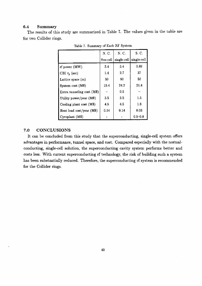
6.4 Summary The results of this study are summarized in Table 7. The values given in the table are
for two Collider rings.
Table 7. Summary of Each RF System.
N. C. N. C. S. C.
five-cell single-cell single-cell
rf power (MW) 3.4 3.4 0.89
CBI Tg (sec) 1.4 2.7 37
Lattice space (m) 50 90 50
System cost (M$) 15.4 24.2 21.4
Extra tunneling cost (M$) - 0.5 -
Utility power/year (M$) 3.5 3.5 1.5
Cooling plant cost (M$) 4.5 4.5 1.8
Heat load cost/year (M$) 0.14 0.14 0.03
Cyroplant (M$) - - 0.5-0.8
7.0 CONCLUSIONS
It can be concluded from this study that the superconducting, single-cell system offers
advantages in performance, tunnel space, and cost. Compared especially with the normal
conducting, single-cell solution, the superconducting cavity system performs better and
costs less. With current superconducting rf technology, the risk of building such a system
has been substantially reduced. Therefore, the supercondUlcting rf system is recommended
for the Collider rings.
43

ACKNOWLEDGEMENTS
The authors would like to thank many rf experts at CgRN, Cornell University, DESY,
Fermilab, and SLAC for their valuable discussions and for other help in the course of this
study. We especially thank Daniel Boussard, Alex Gamp, James Griffin, Joe Kirchgessner,
Phil Morton, Hassan Padamsee, Flemming Pederson, Dieter Proch, Joachim Tiickmental,
and Wolfgang Weingarten. The encouragement and support from Rainer Meinke are
greatly appreciated.

REFERENCES
1. See, for example, J. Griffin, "RF Cavity Primer for Cydic Proton Accelerators," New
Techniques for Future Accelerators II (RF and Microwave Systems), M. Puglisi, S. Stip
cich, and G. Torelli, eds., Plenum Press, 1989.
2. D. Boussard, "RF Power Requirements for a High Intensity Proton Collider" (parts 1
and 2), CERN SL/91-16, (RFS), April 1991.
3. F. Pederson, "Beam Loading Effects in the CERN PS Booster," IEEE Trans. Nucl. Sci.,
Vol. NS-22, No.3, June 1975.
4. D. Boussard, "Control of Cavities with High Beam Loading," IEEE Trans. Nucl. Sci.,
Vol. NS-32, No.5, October 1985.
5. A. Gamp, "Servo Control of RF Cavities Under Beam Loading," DESY HERA 91-09,
May 1991.
6. Conceptual Design of the Superconducting Super Collider (CDR), J.D. Jackson, ed.,
SSC Report No. SSC-SR-2020, March 1986.
7. D. Boussard, "RF Power Estimates for a Hadron Collider," CERN internal report
CERN /SPS/ ARF /DB/GW /Note/84-9, February 1984.
8. F.J. Sacherer, "A Longitudinal Stability Criterion for Bunched Beams," Proc. Particle
Accelerator Conf., San Francisco, March 5-7,1973, IEEE Trans. Nucl. Sci. NS-20, No.3,
June 1973.
9. J.L. Laclare, "Bunched Beam Coherent Instabilities," CERN Accelerator School Pro
ceedings, Advanced Accelerator Physics, CERN 87-03, April 21, 1987.
10. M.S. Zisman, S. Chattopadhyay, and J.J. Bisognano, "ZAP User's Manual," LBL inter
nal report LBL-21270, ESG-15, December 1986.
11. Jorn Jacob, "Measurement of the Higher Order Mode Impedance of the LEP Cavities,"
European Synchrotron Radiation Facility internal report ESRF-RF /88-02, Grenoble,
January 1988.
12. R.D. Kohaupt, private communication.
13. D. Boussard, "RF Technology for pp," CERN Accelerator School Proceedings, Antipro-
tons for Collider Beam Facilities, CERN 84-15, December 20, 1984.
14. G. Schaffer, "RF Cost Figures for the SSC-Collider Rings," April 10, 1992, unpublished.
15. E. Haebel and D. Proch, private communication.
16. L. Emery, "Coupled-Bunch Instabilities in the APS Ring," Proc. 1991 IEEE Particle
Accelerator Conference, San Francisco, May 6-9, 1991.

17. J.F. Bridges, et al., "Measurements on Prototype Cavities (352 MHz) for the Advanced
Photon Source (APS)," Proc. 1991 IEEE Particle Accelerator Conference, San Francisco,
CA, May 6-9, 1991.
18. T.L. Smith, "Mode Identification & Cavity Stretching for the Prototype Storage Ring
Cavity," Argonne Light Source note LS-194.
19. J.F. Bridges, et al., "High Power Testing ofthe Prototype Accelerating Cavity (352 MHz)
for the Advanced Photon Source (APS)," presented at EPAC 1992, Hamburg, Germany,
March 24-28, 1992.
20. G. Cavallari, et al., "Coupler Developments at CERN," presented at the Third Workshop
on RF Superconductivity, Argonne, IL, October 12-21 1987.
21. E. Haebel and J. Sekutowicz, "HOM Coupler Studies at DESY," DESY internal report
M-86-06, July 1986.
22. E. Haebel, "RF Design (Higher Order Modes)," presented at Joint US/CERN Accel
erator School on Factories with e+e- Rings in the series Frontiers of Particle Beams,
Benalmadena, Spain, Oct. 29-Nov. 4, 1992.
23. P. Morton, private communication.
24. A. Gamp, P. Morton, private communication.
25. D. Boussard, private communication.
26. D. Proch, private communication.
27. E. Haebel, private communication.
28. T. Lundin, private communication.
29. G. Conway, private communication.
30. D. Plant, private communication.