A comparison between LSTM and FacebookProphet models: a financial forecasting casestudy

Alejandro González MataGrau en Enginyeria InformàticaIntel·ligència Artificial

Consultor/a: David Isern AlarcónProfessor/a responsable de l’assignatura: Carles Ventura Royo

Gener 2020

Aquesta obra està subjecta a una llicència deReconeixement 3.0 Espanya de CreativeCommons

FITXA DEL TREBALL FINAL

Títol del treball:A comparison between LSTM and FacebookProphet models: a financial forecasting casestudy

Nom de l’autor: Alejandro González Mata

Nom del consultor/a: David Isern Alarcón

Nom del PRA: Carles Ventura Royo

Data de lliurament (mm/aaaa): 01/2020

Titulació o programa: Grau en Enginyeria Informàtica

Àrea del Treball Final: Intel·ligència Artificial

Idioma del treball: Anglès

Paraules clauLSTM, Facebook Prophet, financialforecasting

Resum del Treball (màxim 250 paraules): Amb la finalitat, contextd’aplicació, metodologia, resultats i conclusions del treball

La predicció d’actius financers és una de les principals aplicacions del’Aprenentatge Automàtic i les Xarxes Neuronals. En concret, les xarxesbasades en Long Short-Term Memory (LSTM) han demostrat ser especialmentútils en aquest camp i en altres problemes de sèries temporals. Per contra, s’hainvestigat menys sobre l’idoneïtat i el rendiment del model Facebook Prophet,basat en el model additiu i que és capaç d’unir tèndencies no lineals ambestacionalitats configurables. Aquest projecte buscava construir i comparar dosmodels: un basat en un xarxa neuronal LSTM i l’altre basat en l’algorismeProphet, per així analitzar quin dels dos actuava millor com a predictor, enconcret sobre el preu de l’índex borsari S&P500. Per tal de comparar aquestsmodels un mòdul de simulació de trading va ser implementat i utilitzat com aplataforma de backtesting, mitjançant el qual els models poguessin posar enpràctica les seves prediccions i així determinar el seu rendiment econòmic.Després de l’anàlisi dels models, es va concloure que que la LSTM aconseguiamillors resultats i actuava com un predictor decent en comparació amb altresestràtègies de trading senzilles. El model Prophet també tenia retornsd’inversió positius, però era menys robust com a predictor. A banda, elprojecte ha demostrat la utilitat de fer ús d’una plataforma de backtesting enqualsevol tasca de predicció financera, ja que ajuda a detectar asimetries entreel rendiment d’un model durant la fase de test de l’algorisme i el posteriorrendiment del model en un entorn de trading simulat.

i

Abstract (in English, 250 words or less):

Finance forecasting is one of the main applications of Machine Learning ingeneral and Artificial Neural Networks in particular. Long Short-Term Memory(LSTM) networks have been proven specially useful in this field and in othertime series problems. However, less literature has been written about the suitability and performance of the Facebook Prophet model, which is based onan additive model that blends non-linear trends with configurable seasonalities.This project aimed to build and compare two predictive models, one based on aLSTM network and another one based on the Prophet algorithm, to analysewhich of them performed better in forecasting tasks, particularly in predictingthe price of the S&P500 index. In order to compare these two models, a tradingsimulator module was built as a backtesting platform where the predictions ofthe models could be applied to determine its economic performance. Afterbuilding the two models, it was demonstrated that the LSTM model achievedbetter results, and was proven a decent predictor compared to other benchmarktrading strategies. The Prophet model also showed positive returns ofinvestment, but its accuracy as a predictor was not as high. The project resultsalso suggest that a backtesting platform is a convenient feature when dealingwith forecasting enterprises, since it allows to detect asymmetries between thefitness of a model during the testing phase of the algorithm and its laterperformance in a simulated trading environment.

ii

Table of Contents1. Introduction.......................................................................................................5

1.1 Context and justification...............................................................................51.2 Objectives....................................................................................................61.3 Methodology................................................................................................71.4 Work plan.....................................................................................................71.5 Summary of the products.............................................................................81.6 Chapter description......................................................................................8

2. Tools and data preparation.............................................................................102. 1 Tools selection..........................................................................................102.2 Data gathering...........................................................................................102.3 Data pre-processing...................................................................................112.4 Data presentation.......................................................................................11

3. LSTM model....................................................................................................143.1 How does a Neural Network work?...........................................................143. 2 A brief history of Neural Networks............................................................153.3 The LSTM cell............................................................................................163.4 Hyperparameter description......................................................................173.5 Hyperparameter selection..........................................................................193.6 Data preparation........................................................................................213.7 Hyperparameter tuning..............................................................................223.8 LSTM selected model................................................................................28

4. Facebook Prophet model................................................................................294.1 Model overview..........................................................................................294.2 Hyperparameters.......................................................................................304.3 Default hyperparameters execution...........................................................304.4 Hyperparameter tuning..............................................................................334.5 Logarithmic transformation of the original dataset....................................384.6 Facebook Prophet selected model............................................................40

5. Trading simulator module...............................................................................425.1 Module description.....................................................................................425.2 Additional trading strategies studied..........................................................445.3 Trader simulator testing.............................................................................445.4 Models comparison....................................................................................45

6. Conclusions.....................................................................................................477. Bibliography....................................................................................................49

3

Figure Index Figure 1: Gantt diagram of the project.................................................................7 Figure 2: Daily closing prices of the S&P500 index...........................................12 Figure 3: Training-testing data split...................................................................13 Figure 4: Histogram with the closing prices of the whole dataset.....................14 Figure 5: Neuron diagram..................................................................................16 Figure 6: Comparison between RNN cell and LSTM cell..................................18 Figure 7: Example grid search dictionary defined in Python.............................20 Figure 8: Different learning ratios and its effect.................................................21 Figure 9: LSTM layers distribution.....................................................................22 Figure 10: Training dataset vector with time-step..............................................23 Figure 11: LSTM model 1..................................................................................24 Figure 12: LSTM model 2..................................................................................25 Figure 13: LSTM model 3..................................................................................27 Figure 14: LSTM model 4..................................................................................28 Figure 15: LSTM model 5..................................................................................29 Figure 16: Prophet model prediction with default hyperparameters..................32 Figure 17: Prophet components default hyperparameters................................33 Figure 18: Prophet prediction 1.........................................................................36 Figure 19: Prophet prediction 2.........................................................................37 Figure 20: Prophet prediction 3.........................................................................37 Figure 21: Prophet prediction 4.........................................................................38 Figure 22: Prophet prediction 5.........................................................................41 Figure 23: Prophet prediction 6.........................................................................42

4

1. Introduction

1.1 Context and justification

Since the appearance in the 1970s of the DOT systems (DesignatedOrder Turnaround), that only forwarded trading orders, the trading markethas experimented a huge change thanks to software and computerscience.

From the implementation of systems to assist in decision taking toautomated trading systems (ATS), which automatically take decisionsbased on a set of rules, finance has found in software a powerful tool.The exact percentage is hard to confirm, but something around 60% ofthe trading activities in the equities and the foreign exchange markets [1]are operated by computers.

In this intersection between trading and computing, the field of marketanalysis and finance forecasting has experienced an interesting war ofideas:

There are two main approaches to market analysis: technical andfundamental analysis, which in their core are the exact opposite of eachother. Technical analysis believes that the future prices of an asset canbe predicted by its past price, and frequently make use of statistical andmathematical methods. Fundamental analysis, on the other hand, claimsthat future behaviour of an asset is better predicted from the study of itsfinancial reports and a set of related factors (the environment, thecompetitors, the rest of the economy…).

Until this moment, Machine learning has been widely used mostly intechnical analysis. Since the explosion of neural networks, and speciallyof Recurrent Neural Networks (RNN), lots of research have beenconducted to compare performance of different approaches andalgorithms. In this regard, RNNs and Long Short-Term Memories (LSTM)have been fairly studied [3], [4] as market forecasters.

However, in 2017 a new tool for predicting time series was open sourcedby Facebook: Facebook Prophet tool [21]. This model has already beenused in very interesting applications like Land-Use/Land-Cover

5

classification [25] and others, but has not been as extensively studied asa market forecaster as neural networks.

This projects aims to dig into this recent tool, Facebook Prophet, andexplore its performance as a forecaster. To do so, it will be comparedagainst a solid time series predictor, that has been proven to work well instock market forecasting: LSTMs. Both models will be generated fromscratch as part of the process of understanding and exploring theirrespective strengths.

The motivation for this project is to explore a field where algorithms arerapidly replaced by more efficient ones and where solutions hardly everwork well for all problems.

The Standard & Poor’s 500 index (S&P500) was the variable chosen toforecast. It was chosen between other stock market indexes because it isbroad enough to capture the economic situation of the United States (asopposed to Dow Jones, for instance, which only contains 30 companiesand only from the industrial sector) and because it is commonly used byeconomists as a benchmark1.

1.2 Objectives

This project has two main objectives:

The first one is to implement two different predictive models for the priceof the S&P500 stock index, one of them based on a LSTM neuralnetwork and the other one based on the Facebook Prophet forecastingtool. Those two predictive models will be compared in terms ofperformance between them and also with other trading strategies that willbe used as benchmarks.

The second main objective of this project is to implement a tradingsimulator module in Python where the predictive models can apply theirpredictions with real-world data. This tool will also be used to evaluatethe models’ performance.

1 Benchmark is a model or measurement against which to compare the performance ofanother model.

6

1.3 Methodology

The project involves generating and comparing two predictive models,the architectures of which will be designed and subsequently tuned fromscratch.

The process will be inherently iterative. The models will be firstgenerated with default hyperparameters and they will be updatedgradually in order to find the best performing ones.

1.4 Work plan

The original idea for the project suffered a deviation during November.The objective has always been to build a predictive model, but originallythe method to generate this model was to make use of aneuroevolutionary algorithm called NEAT, and it was exclusively focusedon neural networks.

After the project goal shift, the planning was changed and most of themilestones were modified. The Gantt diagram in Figure 1 shows theproject’s tasks after the change: some of the older project tasks werereused (the data gathering and pre-processing, the LSTM modelpreparation), but some of them were not.

7

Figure 1: Gantt diagram of the project

1.5 Summary of the products

Besides this report, containing the numerical results of the comparisonbetween the two models, the second product generated is the tradersimulator and the rest of the Python project needed to generate themodels and interpret them.

This Python project consists mainly of:

• lstm.py: the module which performs the training and testing of the LSTMmodels.

• prophet.py: the module which performs the training and testing of theFacebook Prophet models.

• trader_simulator.py: the module that interprets the models generated andperforms the trading simulation.

• data_preprocessor.py: an auxiliary module containing methods for datamanipulation.

• test/test_trader_simulator.py: the unit test implemented to verify thetrader simulator.

Some models and predictions (.h5 and .csv files) and plots were alsoincluded in the project’s folder structure, together with the original dataset(sp5001962.csv) used for this project and a README.txt file explainingthe different modules.

1.6 Chapter description

Chapter 2 presents the data used for the prediction task and details thepreparation process. It also enumerates the tools used and the criteriabehind this selection.

Chapter 3 describes the process of building the LSTM model, as well asthe basics about Neural Networks, Recurrent Neural Networks and theLong Short-Term Memory cell.

Chapter 4 does the same process description for the Facebook Prophetmodel.

8

Chapter 5 explains the trader simulator module and how it compares theperformance of the models, finally presenting the results of each model’sprediction.

Chapter 6 presents the conclusion of the project.

9

2. Tools and data preparation

This chapter contains information about the tools used in this project andexplains the methods applied to the original dataset in order to prepare it for theconstruction of the models. It ends with a visual presentation of the data.

2.1 Tools selection

The code for the project was written in Python [6].

For the implementation of the LSTM, two libraries were considered: TensorFlow[7] and Keras [8]. Keras runs on top of TensorFlow and it is a higher levellibrary, so it is faster to prototype and build different architectures with it.TensorFlow also has a high-level API and provides more features, but as theproject would not make use of those features, Keras was chosen for itssimplicity.

For the Facebook Prophet model, the implementation in Python was used.

Some other libraries were used, the most important of them being: sklearn(used for preprocessing tasks), matplotlib (for plotting), numpy (for arrayhandling) and pandas (for reading and writing the datasets).

2.2 Data gathering

Unlike intraday stock prices (with periods smaller than a day, i.e., seconds,minutes our hours), which tend to be hard to find or expensive, daily data isubiquitous and free. The most common dataset for the stock index S&P500 isthe OHLC set, which refers to Open-High-Low-Close prices: the prices at theopening and closing time of the stock market, and its highest and lowest valueachieved during that period. It can be found in several websites.

For this project, the data used was extracted from Yahoo! Finance [5], and itcovers from 2nd January 1962 to 5th December 2019. Stock markets are closed

10

on weekend days and holidays, and the downloaded dataset already considersthat information. Therefore, the days in which the stock market is closed do notappear as samples in our data, which means that the total number ofobservations is 14583.

2.3 Data pre-processing

Since the time series predictive models that are going to be built are univariate,only one column from the OHLC will be selected, the rest will be ruled out.Closing price is the one feature that will be observed since it includes theinformation of the day and would eventually allow the trading simulatror toperform its calculation during the closing times of the stock market (night) andplace a buy or a sell order during that time.

Once the dataset contains only the closing price for each observation (day),some sort of data normalization should be made. This normalization is frequentin Machine Learning tasks and consists in transforming the data in order tomake fit it in a smaller range.

This data transformation has been largely proven to make models not only trainfaster, but also to achieve better performances. In this project, some sort ofnormalization will be applied to both models built, but for each model thetechniques used will be different: in the case of the LSTM model, Min-Maxnormalization will be applied. For Prophet, on the other hand, a logarithmictransformation will be carried out. However, each of these methods will beexplained in the respective chapters for each model.

Lastly, it is worth pointing out that for the LSTM model the train dataset and thetest dataset will be slightly smaller than the original one. This happens becausethe LSTM needs the observations of the N previous days to perform aprediction for the next one. That means that the first prediction that the LSTMwill be able to make is for the observation number N+1 of the test dataset.However this will be thoroughly explained in Chapter 3, and does not have agreat effect in the results, since N will be small.

11

2.4 Data presentation

The dataset after the pre-processing carried out in the previous chapter showthe following values:

The range of the closing prices goes from 52.32$ on its lowest value inFebruary 1962, to 3,153.63$ in November 2019, when it reaches its maximum.

This dataset needs now to be split in training and testing dataset in order to beable to validate the models built in the following chapters. The first 80% of theobservations will serve as training set and the last 20% will be used as testingset.

This draws the split line the on the 7th May 2008:

12

Figure 2: Daily closing prices of the S&P500 index between 1962 and 2019

And it means that the train dataset will contain 11666 observations, while thetest dataset will contain the last 2917 observations.

Another data visualization plot that will be useful to better understand thedataset is the histogram with the frequencies of the different closing priceranges:

13

Figure 3: Training-testing data split

As it could be noticed in the previous plots, most of the samples of the datasethave values smaller than 1,500$, and there is a big mode in the first bin of thedistribution. This knowledge will prove useful when normalizing the data for therespective models.

14

Figure 4: Histogram with the closing prices of the whole dataset

3. LSTM model

In this chapter there is a short introduction to neural networks: how they workand its history. There is also a presentation of the LSTM cell or unit and thehyperparameters that can be used to define a network based on it.

After this theoretical presentation, the LSTM predictive models generated forthis projected are presented and compared with each other. Finally, there is asummary of the selected model with its hyperparameter configuration.

3.1 How does a Neural Network work?

A neural network is a machine learning system, composed of artificial neuronsconnected with each other. Those neurons perform a transformation in a set ofinputs to generate outputs, which can be used both in tasks of classification orregression.

The learning aspect of a neural network takes place after every iteration duringthe training phase, and it mainly updates the relationship between neurons sothat the network can globally adjust better to the expected outputs.

The inner working of a single neuron is the following (see Figure 5):

15

A neuron receives different input values from different neurons (x1...xn). Eachone of this connections with other neurons has a weight assigned (w1...wn), thatcan be updated during the training phase to minimize the difference betweenthe output of the neural network and the expected output.

Inside the neuron, the calculations taken place are:

y neuron=f (∑j=1

n

x j∗w j+b) (1)

Where x are the input values from other neurons, w are the weights, b is thebias value and f is the activation function, which modifies and normalizes theoutput and can be of different types.

3. 2 A brief history of Neural Networks

The idea behind neural networks was born in 1943 by the neurophysiologistWarren McCulloch and the mathematician Walter Pitts, who proposed atheoretical model to represent the inner working of biological neurons withpropositional logic [11]. This served as a starting point for a series of newinventions:

16

Figure 5: Neuron diagram. Source: https://towardsdatascience.com/statistics-is-freaking-hard-wtf-is-activation-function-df8342cdf292

In 1958, the perceptron was presented by Frank Rosenblatt. Perceptrons areprimitive neural networks that only have an input and an output layer consistingof linear threshold units (LTU), which perform a weighted sum of theconnections that they receive from other units and then apply a step function.This is the main behaviour of neurons and despite being very limited in terms ofarchitecture and learning, the perceptron already reinforced the connectionsthat lead to lower errors in the final predictions.

Some years later, in 1986, D.E.Rumelhart et al. [12] presented thebackpropagation algorithm, which made training much more efficient. Thisalgorithm is very clearly described by A. Géron in p. 263-264 of his book“Hands-On Machine Learning” [17]:

“For each training instance the backpropagation algorithm first makes aprediction (forward pass), measures the error, then goes through eachlayer in reverse to measure the error contribution from each connection(reverse pass), and finally slightly tweaks the connection weights toreduce the error (Gradient Descent step).”

Then, Recurrent Neural Networks (RNN) appeared. As opposed to infeedforward networks, the neurons in recurrent networks are connected tothemselves across time steps. This means that a neuron, in addition to theconnections with other neurons, is also connected to its past state, thusallowing the network to develop some sort of memory.

3.3 The LSTM cell

The Long Short-Term Memory cell (or unit) appears as an extension of the RNNcell. It has been modified and extended since its presentation paper by S.Hochreiter and J. Schmidhuber [14], but the main components can still beobserved in Figure 6:

17

The x vector and the h vector work as the input and the output vector of asimple neuron respectively. However, there are several more differences.

In the first place, there are two more input vectors to the cell: ht-1 and ct-1. Thosetwo values represent respectively the short and the long-term state of theprevious time step cell. This way, ht is at the same time the output of the currentunit and the short-term input for the next time step cell.

The main idea behind the LSTM unit is that it allows a long-term vector c to flowover time steps, dropping and learning new memories (via the Forget andOutput gate), while at the same time also the short-time h memory is beingused by the unit.

3.4 Hyperparameter description

A LSTM network has several hyperparameters that can be tuned. Thepreeminent amongst them are:

• Batch size: defines the number of samples that go through the networkbefore the inner parameters of the network update themselves. Eachupdate on the inner parameters is called an iteration so, in a way,defining the batch size equals to define the number of iterations in eachepoch.

18

Figure 6: Comparison between RNN cell and LSTM cell. Source: [9]

For instance, with a training dataset of 11520 observations, having abatch size of 96 samples will allow the neural network to update itself120 times (iterations).

1152096

=120 (2)

• Number of epochs: defines the number of iterations over the wholetraining dataset.

• Number of layers: layers are divided into input, hidden and output ones,and are aggregations of neurons. But as a hyperparameter, the numberof layers refers only to hidden layers.

• Units per layer: refers to the number of neurons in each layer.

• Input sequence’s length (also called time steps): the number ofobservations into the past that each sample contains.

• Objective function (or loss function): the function that computes thedifference between the predicted output and the actual one, i.e., thefunction that the neural network is trying to minimize. For this project,since the objective is to minimize the error, it will referred as the lossfunction.

• Optimizer: the optimization function is the mechanism that uses theneural network to find the value that minimizes the loss function. One ofthe most important optimization algorithms is Stochastic GradientDescent (SGD), which relies on the iterative calculation of the gradient ofa function, making steps at each point towards the negative gradient inorder the find the global minimum.

There are however more recent algorithms that extend and modify thisapproach, like AdaGrad o Adam, and which converge faster and findbetter minima because of its finer behaviour in sparse gradients (thatappear, for instance, when approaching the minimum) [15].

• Dropout: is a technique proposed by Srivastava et al. [10] whichaddresses the problem of overfitting. It does it by randomly disabling(dropping) different units in a neural network along with their connectionsduring training. This prevents the system from relying too much in somespecific units, thus becoming too specialized.

19

3.5 Hyperparameter selection

In order to test several combinations of the previously defined hyperparameters,a grid search dictionary was defined. This dictionary (see Figure 7) is later usedwith the help of the scikit-learn library [24] and allows to test the model with allthe possible combinations of variables defined in the dictionary.

The grid search was performed to find the combination that achieved the lowererror in the test dataset. Specifically, the hyperparameters tested were:

• Input sequence length (or time steps): for this dataset, where everyobservation is a day, they were considered time windows of [5, 150] daysin the past.

• Number of units: this is, the number of LSTM cells in each hidden layer.The range of values tested was [5, 500].

• Number of epochs: values between [3, 50] were tested.

• Batch size: values between [32,128] were tested.

• The number of layers: the range of [1, 4] hidden layers was tested.However, since 2 layers early appeared to be the most efficientarchitecture, all the experiments presented in this section have theconstant value of 2 hidden layers. The results in Table 1 also refer to a 2hidden layer architecture.

The rest of the hyperparameters were not included in the grid search andtherefore had constant values:

• Loss function: mean squared error has been chosen:

20

Figure 7: Example grid search dictionary defined in Python

MSE=1N∑

i=1

N

(Y i−Ŷ i)2

(3)

where N is the number of predictions, Y is the vector of observed valuesand Ŷ is the vector of predicted values. It is a function that highlypenalizes outliers because of the 2-exponent.

Mean absolute error could have also been chosen as the loss function,but in this case it was considered desirable that the model punishedlarge errors specially. Furthermore, mean absolute error was also testedbriefly as loss function for this experiment, and it generated slightly lessaccurate models.

• Optimizer: Adam algorithm was chosen. There are two main reasons:first of all, for its adaptive learning rate. The learning rate determines thespeed at which the model changes as a response to the loss function.For optimization algorithms based in gradient descent, the learning ratedetermines the size of the step towards the minimum that the system willtake (see Figure 8).

Considering θ the variable studied and J(θ) the loss function to minimize,we can see the effects of the learning rate: a rate too high means a riskof overshooting the minimum, even a risk of diverging (left image), and arate too low means a risk of getting stuck at global minima or slowconvergence (right image).

21

Figure 8: Different learning ratios and its effect. Left image: high learning rate. Centerimage: adequate learning rate. Right image: small learning rate. Source: self-elaboration

Adaptive learning rates appeared to try to solve this problem and will bethe choice for this project.

Secondly, Adam was chosen among other adaptive learning-ratealgorithms for its faster convergence [15], [16].

• Dropout probability: 20%. Dropout was incorporated into the model byadding a Dropout Keras layer after each LSTM layer. This way, for eachiteration over the network, 20% of the units in each LSTM layer will bedisabled and not taken into account for the weight updates.

The final distribution of the LSTM layers can be seen in Figure 9: two hiddenLSTM layers with dropout, and an output layer with an only unit (only onefeature is being predicted, that is the closing price, so the output layer will haveonly one unit).

3.6 Data preparation

The data to feed the neural network with must have a particular shape.Specifically, Keras needs the train dataset to be a 3-dimensional vectorcontaining (number of samples, time-steps, number of features):

The number of time-steps will be one of the hyperparameters to be tuned andthe number of features will be always one, since the time series model we areworking with is univariate (it has only one feature, the closing price of theS&P500).

In this case, the number of samples will be the train dataset (11666) minus thenumber of time-steps. This happens because the LSTM model needs the Nprevious observations to perform a prediction (see Figure 10):

22

Figure 9: LSTM layers distribution

The first value that it will be able to predict will therefore be the N+1th

observation, thus reducing the train dataset by N observations. This will not beproblematic since, as it will be showed in subsequent chapters, the optimalvalue for N is quite small (N=5).

Other than that, data is also normalized by using the MinMaxScaler from thesklearn library [24], which uses the following formula:

X std=X−X .min

X .max−X .min(4)

X scaled=X std∗(max−min)+min (5)

where X.min, X.max represent the minimum and maximum values in the originaldata and min, max the desired range, in this case (0,1).

This is a very common choice because, as opposed to standardization (zero-mean and unit variance), it does not distort the data.

The Scaler is fitted with the training data and then both training and test dataare transformed. The transformation will be inverted after training the model, sothe data can be visualized and studied with their original values.

3.7 Hyperparameter tuning

23

Figure 10: Training dataset vector with time-step. Source: self-elaboration

In order to measure the fitness of a model, a lot of metrics can be chosen. Forthis project (both for the LSTM and for the Facebook Prophet model), theselected function will be the root mean squared error (hereafter RMSE), whichis the square root of the MSE defined in formula (3):

RMSE=√ 1N∑i=1

N

(Y i−Ŷ i)2

(6)

Mean absolute error (MAE) could have also been used, since it has theadvantage that it is more intuitive and presents directly the mean of the errors:

MAE=1N

∑i=1

N

|Y i−Ŷ i| (7)

However, let us recall that the model was built using MSE as the loss function inorder to penalize large errors. Although a different metric could have been usedhere to measure the predictions error, RMSE was also chosen so that thispenalization was also taken into account when evaluating the model. Inaddition, RMSE has the advantage that it acts as an upper bound to MAE andtherefore it already gives some information about it.

Before analysing the concrete results of the search grid, there is a phenomenonworth mentioning:

The models that yield a better RMSE seem to predict the real values someobservations later, which means that the predicted value is something similar toa shift of N observations to the right (see Figure 11 and Figure 12). This isdifficult to avoid because this kind of behaviour actually performs well, but itavoids the possibility of finding a more generic predictor that could performworse in terms of the loss function, but rather behave in a more visionary way.

24

However, the models that show this kind of behaviour are not an absolute shiftof N observations. As it can be sen in Figure 12, which shows an extract ofFigure 11 between observations [200,300], the predicted function is notcompletely overfitted.

25

Figure 11: LSTM model with input_seq=5, units=200, epochs=5, batch_size=64

Figure 12: LSTM model with input_seq=5, units=200, epochs=5,batch_size=64. Zoomed over observations [200,300]

This shift can be observed in other models built with neural networks for timeseries prediction. For instance, the neural network built by A. HedayatiMoghaddam et al. [18] for the NASDAQ stock price prediction also show thatdeviation.

The existence of this phenomenon was a motivation to implement a tradingstrategy (that will be explained in Section 5.2) that assigns to the prediction forthe next day the value of the Nth previous one (in this case, N = 5 will be useful).This simple strategy will be useful to compare its performance particularly withthe LSTM model.

Other than that, it can also be interesting to calculate the RMSE between thereal values and a theoretical shift of X observations in that data. Having X=1day, the RMSE obtained is 36.50:

RMSE=√ 1N∑i=1

N

(Y i−Y (i−1))2=36.50 (8)

However, having X=5 days, which is more or less the deviation that theobtained model seems to have, the RMSE obtained is:

RMSE=√ 1N∑i=1

N

(Y i−Y (i−5))2=79.49 (9)

This values will serve as a benchmark for the LSTM models generated. Forinstance, the LSTM model referenced in Figure 11 has a RMSE of 41.31 whichmeans that it performs slightly worse than the 1-day shift just calculated asbenchmark, but better than if was just a 5-day shift in the data.

Having explained this phenomenon and having the 5-day shift RMSE asbenchmark, the grid search results are presented (see Table 1):

26

Inputsequence

lenth

Number ofunits

Number ofepochs

Batch size RMSE

5 5 5 96 532.30

5 10 8 96 399.25

5 150 5 128 43.14

5 200 3 64 37.71

5 200 5 64 41.31

5 200 8 64 139.26

5 500 3 1 307.83

5 500 5 96 33.87

5 500 8 96 35.56

5 500 50 96 135.61

10 50 5 64 168.61

10 500 5 128 37.37

15 200 5 128 46.11

15 500 5 96 47.89

20 50 5 64 226.62

60 500 3 64 85.44

60 500 5 64 148.56

60 500 8 64 74.27

60 500 3 96 83.53

60 500 5 96 37.07

60 500 8 96 84.82

100 50 5 64 188.33

100 200 5 64 59.08

120 150 5 64 92.42

120 200 5 64 63.17

120 500 5 64 78.37

Table 1: RMSE of the LSTM models

The conclusions that can be extracted from this data and from the plots are thefollowing:

• Input sequence length, i.e., a long window into the past, does notcorrelate positively with accuracy. The grid search shows that for both

27

sequences of 5 or 60 observations into the past, the results are quitesimilar.

• It seems beneficial for the model not to train a lot: a higher number ofepochs generates bigger errors. Let us see the best model (Figure 13)which was trained during 5 epochs, compared with the model that hasthe same configuration but trained during 50 epochs (Figure 14):

28

Figure 13: LSTM model input_seq=5, number_units=500, epochs=5,batch_size=96

The model trained for 50 epochs performs way worse specially in the lastpart of the test set. This might be caused by an overfitting acquired overthe train dataset, which has way lower prices that the test dataset. Thoselower values might have been learned by the network, but this is just anhypothesis.

• Low input sequences work well with a high number of units. If thenumber of units is also low (for instance input_sequence=5 andnumber_neurons=10), the model captures the trends, but fails to adjustthe value (see Figure 15).

29

Figure 14: LSTM model input_seq=5, number_units=500, epochs=50,batch_size=96

• In general, both for short and long input sequences, a high number ofunits is needed to let the model learn from the data.

• The adequate batch size for this experiment seems to be 96. They werealso tested extreme batch sizes like 1 that did not perform well despite itsvery high computational cost.

3.8 LSTM selected model

The best performing model, i.e. the model with the lower RMSE, is the one withthe following hyperparameter configuration:

• Input sequence length: 5• Number of units: 500• Number of epochs: 5• Batch size: 96

Its RMSE over the test set is 33.87, which is slightly better than the benchmarkvalue of 36.50 obtained in Formula (8), by calculating the RMSE of the test setwith its 1-observation shift to the past. But it is way better in terms of error thanthe 5-observation shift calculated in Formula (9), which was 79.49.

30

Figure 15: LSTM model input_sequence=5, number_units=10

For a more detailed exploration of the model’s fitness, the MAE was alsocalculated (Formula 7) and the resulting value was 24.92.

31

4. Facebook Prophet model

In this chapter the Facebook Prophet implementation is presented, as well as itsmain hyperparameters tuned to generate the predictive model for the project.

A first execution was carried out with the default parameters of the algorithm, tosee how it performed without any changes. After that, more executions werecarried out: firstly, the original dataset was fed into the algorithm without anydata normalization process. After that, a logarithmic transformation was carriedout on the original dataset, with the purpose of determining the suitability of it,while trying to search for better models.

At the end of the chapter there is a summary of the hyperparameters of theselected model.

4.1 Model overview

Facebook Prophet is a model and a library that provides features both fromgeneralized linear models (GLM) and additive models (AM), mainly extendingGLM by using non-linear smoothing functions. It was specified by Taylor andLetham [19] in 2017.

The main difference between Prophet and other statistical methods is theanalyst-in-the-loop approach. This approach allows the the analyst to apply theirdomain knowledge about the data to the forecasting algorithm, without havingany knowledge of the statistical methods working from within. This approach,therefore, tries to take advantage from both the statistical forecasting and thejudgmental forecasting, the latter being the forecasting methods based onhuman experts decisions. The parameters that can be tuned by the analyst willbe defined and explained in sections 4.2 and 4.4.

The general function to define the time series is the following:

y (t )=g(t )+s(t )+h(t )+ϵt (10)

32

where g(t) represents the non-periodic changes in the value of the time series,s(t) model seasonality (which can be daily, weekly, monthly, yearly or anyother), h(t) represents the effects of holidays and εt is the error term.

4.2 Hyperparameters

There are several customizable parameters in Facebook Prophet’simplementation [21], the main ones being:

• Changepoints: which define trend changes. These can be found by thealgorithm itself or they can also be defined and tuned by the analyst.

• Seasonality: which define the periodic functions which may affect thetime series. By default, Prophet considers yearly, weekly and dailyseasonality, and tries to find trends that represent those periodic effectsin data.

• Holidays: special days (holidays or any other recurrent event) can alsobe modeled by the Prophet additive model. The dates can be addedmanually through a pandas.Dataframe, but there are also built-in holidaysets for a dozen countries.

• Fourier order: referring to the seasonality function, this value willdetermine how fast it can change and adapt, and it will also imply a morefitted model (with the consequent risk of overfitting).

From these hyperparameters, holidays was the only one that was not tuned orconsidered for the building of the current model. There are two reasons for thisdecision: first of all, the S&P500 is a highly globally operated index, andtherefore it is not self-evident that considering only one country’s holidays wouldmake an important difference. But most importantly, equities market are closedon United States holidays, so our original S&P500 dataset does not contain anyinformation in these days for the algorithm to model.

4.3 Default hyperparameters execution

33

Having discarded the holidays, executing the default configuration generatesthe following Prophet model, which can be plotted with the built-in plot function:

The black line shows the training data and the blue line shows the predictionmade (both for the training and the test data, which consist in 2817observations). The lighter blue area delimits the upper and lower predictionbetween the certainty interval (by default it is 80%).

34

Figure 16: Prophet model prediction with default hyperparameters

As we can see, the model is not finely adjusted during the training phase withthe default configuration, but let us see the decomposed seasonalities toexplain how this feature works:

Prophet has three default seasonalities: daily, weekly and yearly. As our datado not contain intraday data (meaning hourly data or even data with smallerintervals like minutes or seconds), the daily seasonality is directly eliminated bythe library. The other two default seasonalities are printed, besides the generaltrend of the prediction.

Some comments on these periodic trends should be made: first of all, thegeneral trend is not correctly determined from 1999 onwards.

35

Figure 17: Prophet components with default hyperparameters. Top image: trendcomponent effect to the general function. Center image: weekly seasonality

effect. Bottom image: yearly seasonality effect.

Second of all, weekly seasonality takes into account weekend days, which arenot in the original dataset as the stock market is closed. So, using our dataset,weekly seasonality should be disabled in the way that it is defined.

Lastly, the yearly seasonality is indeed interesting as it highlights twophenomena that appear frequently in the economic circles. Those are theSeptember Effect and the January Effect, each one respectively referring to adecrease and an increase in stock prices in those months. The SeptemberEffect seems important in our data, and has higher evidence in economicliterature [20]. The January Effect has a smaller impact, but it is also significant.

4.4 Hyperparameter tuning

Once the default configuration has been proven to not perform well as apredictor, the next step is to tune the configurable hyperparameters previouslydescribed: period of the seasonality, Fourier order of this function andchangepoints.

The first step will be to disable the default Prophet seasonality (weekly, yearly,daily). Prophet allows to make use of several seasonality functions working atthe same time, but after trying to define a model with 2-3 different seasonalityfunctions working at the same time, this option was discarded. The reason isthat, despite being more time and resource intensive, the resulting RMSE didnot seem to get specially lower.

Therefore, all the performance results showed in Table 2 are calculated withonly 1 seasonality function, described by its period and Fourier order. Thevariables and its respective range values considered were:

• Period: this variable determines the number of days in a seasonality, soa wide range of values were tested: [5, 12000].

• Fourier order: the default value is 10 for yearly seasonality, but in thisdataset, the range [3, 25] was tested.

• Changepoints: it is not recommended to change directly the number ofchangepoints, but rather to change the strength of the sparse prior. Boththings were done in this experiment. changepoint_prior_scale was

36

changed between [0.001, 10] and changepoints were changed from [10,100] (from a default number of default of 25). Having tested thatchanging the number of changepoints did not affect a lot the results, thatvariable did remain constant in the default value for the rest of the modelexperimentation.

These variables were evaluated using a grid search over different subsets ofvalues. Also, as with the LSTM, RMSE has been the metric chosen to evaluatethe performance of the model, but the results will also be evaluated visuallyusing plots.

For conciseness reasons, only some of these variable combinations have beencopied into this report:

Period Fourier order Changepointsprior scale

RMSE

7 5 0.05 772.04

7 10 0.05 771.17

7 20 0.05 771.35

20 5 0.05 772.31

20 10 0.05 772.75

20 20 0.05 771.19

1000 5 0.01 775.35

2700 10 0.04 857.12

2750 10 0.05 841.40

2850 5 0.01 788.06

5000 5 0.1 569.73

7500 5 0.1 431.90

7500 5 0.04 325.15

9000 5 0.13 251.61

9000 5 0.1 330.10

9000 10 0.01 429.41

11000 5 0.01 388.55

11000 5 0.1 348.57

11000 5 0.13 430.29

11000 10 0.13 911.60

11000 15 0.01 367.40

Table 2: RMSE of Prophet model with raw data

37

The best RMSE obtained in that grid search corresponds to a model with aperiod of 9000 observations, a Fourier order of 5, a changepoint prior scale of0.13 (higher than the default 0.05) and the default number of changepoints (25).Its plot can be see in Figure 18.

The consequences extracted from these results are:

• Period is the most important variable of all, and has the bigger impact inthe RMSE.

• Fourier order also makes a big impact on the model. In some cases itdoes only adjust the model in a more fitted way, but in other cases, thechange of this value can absolutely change a trend and modifyspectacularly the results, as shows in Figure 19 and Figure 21.

These two models differ only in its Fourier order value, being 15 and 5respectively. And while the Fourier order of 5 seems to capture thepositive trend quite well, the model with Fourier value of 15 predicts anegative trend that does not happen.

38

Figure 18: Prophet prediction with period=9000, fourier_order=5,prior_scale=0.13

• It is difficult to chose a particular combination of variables, because theRMSE, besides being too high, does not reflect well the fitness of themodel. For instance:

39

Figure 20: Prophet prediction with period=2700, fourier_order=5

Figure 19: Prophet prediction with period=9000 and fourier_order=15

Figure 20 shows a RMSE=860.14, while in Figure 21, RMSE=330.10.This could lead us to choose the second model since its performance isway better, but looking into the plots, it seems that the first model does abetter job at identifying change trends, though it fails to correctly predictthe dimension of this change.

Particularly, it detects the 2008 bottom price (even though it detects it toolate and with a higher price) and it also detects a second local minimumaround 2015, while the model in Figure 21 fails to identify these twochange points and has a broader prediction.

• That said, there are two configurations of period that seem to reflect wellour data in two different ways, and those are a period value close to2750 observations (days) and another one around 9000. The latterperforms worse but seems to have a better understanding of trends, andthe former has closer predictions to the real values but fails to getimportant downs in price.

• Lower periods close to one week (period=5, since only workdays aretaken into account) or one month (period=20) do not perform well at alland fail to fit the model during the training phase.

40

Figure 21: Prophet prediction with period=9000 and fourier_order=5

4.5 Logarithmic transformation of the original dataset

The previous section calculations were made without any data pre-processing.But given the high error of the predictor and the skewed distribution of our data,a second model incorporating pre-processing was considered in order to test ifthe model could be more accurately fit during training. As showed in Figure 4,the original dataset shows what could be considered a positive skew, with aremarkable long tail. There is a wide range of values (between 52.32$ and3,153.63$), but most of the samples are concentrated on the lowest part of thedistribution.

For those reasons, it was considered appropriate to apply the logarithmictransformation to the original data as a data pre-processing mechanism. Thiswill allow us to compare the performance of model with and without pre-processing.

Given its mathematical nature, the logarithmic transformation is most usefulwhen data has a range of several orders of magnitude. In this case, data spanstwo orders of magnitude, and has a rather low value for most part of the trainingdata, so it could be beneficial to normalize it this way so that the feature hascomparable values.

As it happened with the LSTM, the data pre-processing is done in thedata_preprocessor.py module. In this case, it consists only of applying thenatural logarithm to the closing price of each day. The model is fit with thetransformed data, but the resulting predictions are re-transformed (in this casewith an exponential function), in order to be able to compare them with theoriginal data. The RMSE is therefore calculated with the re-transformed data, soit can be compared with the other Prophet model and with the real dataset.

The resulting RMSE for the same grid search used in the previous section are:

Period Fourier order Changepointsprior scale

RMSE

7 5 0.05 789.33

7 10 0.05 788.50

7 20 0.05 789.70

20 5 0.05 787.84

20 10 0.05 790.22

20 20 0.05 790.28

41

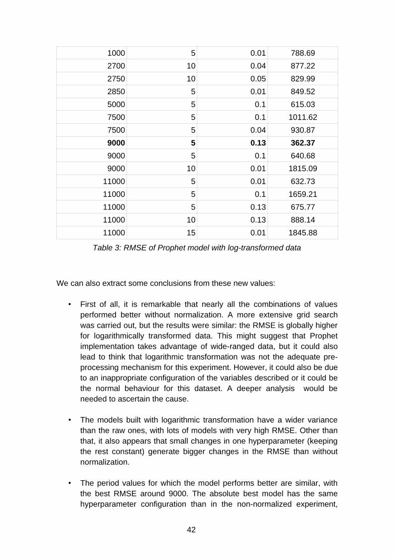
1000 5 0.01 788.69

2700 10 0.04 877.22

2750 10 0.05 829.99

2850 5 0.01 849.52

5000 5 0.1 615.03

7500 5 0.1 1011.62

7500 5 0.04 930.87

9000 5 0.13 362.37

9000 5 0.1 640.68

9000 10 0.01 1815.09

11000 5 0.01 632.73

11000 5 0.1 1659.21

11000 5 0.13 675.77

11000 10 0.13 888.14

11000 15 0.01 1845.88

Table 3: RMSE of Prophet model with log-transformed data

We can also extract some conclusions from these new values:

• First of all, it is remarkable that nearly all the combinations of valuesperformed better without normalization. A more extensive grid searchwas carried out, but the results were similar: the RMSE is globally higherfor logarithmically transformed data. This might suggest that Prophetimplementation takes advantage of wide-ranged data, but it could alsolead to think that logarithmic transformation was not the adequate pre-processing mechanism for this experiment. However, it could also be dueto an inappropriate configuration of the variables described or it could bethe normal behaviour for this dataset. A deeper analysis would beneeded to ascertain the cause.

• The models built with logarithmic transformation have a wider variancethan the raw ones, with lots of models with very high RMSE. Other thanthat, it also appears that small changes in one hyperparameter (keepingthe rest constant) generate bigger changes in the RMSE than withoutnormalization.

• The period values for which the model performs better are similar, withthe best RMSE around 9000. The absolute best model has the samehyperparameter configuration than in the non-normalized experiment,

42

and its plot can be seen in Figure 22, over the transformed data, and inFigure 23, over the re-transformed data.

As it happened with the non-normalized model, it seems to capture sometrends, but it does it too late for some of them (the 2008 crash) and failsto adjust their dimension.

43

Figure 22: Prophet prediction (normalized data) with period=9000,fourier_order=5, prior_scale=0.13. Over the transformed dataset

Figure 23: Prophet prediction (normalized data) with period=9000,fourier_order=5, prior_scale=0.13. Over the de-transformed dataset

4.6 Facebook Prophet selected model

Given that the best performing model with normalization is significantly worsethan its non-normalized equivalent, the non-normalized model will be selectedto be compared with the LSTM model.

Therefore, the hyperparameters for the best model are:

• Period = 9000• Fourier order = 5• Changepoint prior scale = 0.13• Number of changepoints = 25 (default value)

Its RMSE over the test set is 251.61 and its MAE is 191.95.

44

5. Trading simulator module

In order to compare the performance of the models built for the project, atrading simulator was built in which the models can see the financial results oftheir predictions. This trading simulator module is explained in this chapter,alongside some auxiliary trading strategies that were implemented to be usedas benchmarks.

There is a reference to the unit tests written to verify this module, and finallythere is a comparison between the financial returns of all the modelsimplemented (LSTM, Prophet and the auxiliary strategies).

5.1 Module description

Even though the LSTM and the Prophet model could be compared by usingmathematical indicators, another objective of the project was to develop aplatform where these two models could perform as automatic traders. This toolwould act as a backtesting2 module and could be used as a foundation for aneventual system to perform automatic trading on a real-world environment.

The trading simulator uses the same test dataset that was used to tune thehyperparameters and select the more effective LSTM and Prophet predictors,i.e., the data set from the 14th May 2008 to the 5th December 2019. Let us recallthat the original test dataset starts at 7th May 2008, but given the prediction shiftN = 5 that was explained in Chapter 3.6 (see Figure 10) and the lack of samplesfor the weekend days, the first value that can be predicted is the 14th May.

For each day of the dataset, the simulator decides whether to place a buy orderfor the next day, sell or do nothing at all, depending on the predicted value andthe closing price of that day. The decision to buy or sell is taken in a quitestraight-forward and simple way:

If the predicted value of the S&P500 index for the next day is higher than theclosing price of the current day, a buy order is placed. As the simulator has a

2 In predictive models and specially in trading, backtesting is the process of testing a model ora strategy in a secure environment before deploying it in the real world.

45

limited amount of money, it will only be able to buy stock when it has therequired liquidity.

If the predicted value is lower than the closing price of the current day, a sellorder will be placed. Likewise, this order will be carried out only if the traderholds stock in that moment.

At the end of the test dataset, a financial measurement is calculated to show theperformance of each model. The measurement selected is the return ofinvestment (ROI), which is calculated following the formula:

ROI=(Final value of the investment−Cost of investment)

Cost of investment(11)

Summarized, the algorithm behind the module works as follows:

1. An initial capital (10,000$) is assigned to every different model to investit.

2. The test datasets are loaded to perform the comparison with thepredicted values.

3. The predictive models are loaded (in the case of LSTM from the .h5 filesgenerated during the training).

4. The predictions are loaded or generated with the test dataset.

5. Each model executes an specific method to go over all the days in thetest dataset, deciding for each day whether to buy or sell depending onthe prediction made.

6. After going through all the days in the test dataset, the initial capital hasincreased or decreased. The last day, all the stock is sold with theconsequent closing price.

7. A performance ratio is calculated to measure the performance of eachstrategy. In this case, the return of investment or ROI.

46

5.2 Additional trading strategies studied

Besides the LSTM and the Facebook Prophet model, four more models weredeveloped and tested in order to use them as benchmarks for performance.These models were:

• A buy and hold model: this strategy has many advocates amongstfamous investors and makes the case that assets should be held for along time. In our module, this will translate into buying all the stockpossible at the beginning of the test phase and holding it until the verylast day, when it will be all sold.

• Simple Moving Average model (SMA): this method calculates theaverage between the N past observations and assigns the calculatedvalue to the prediction for the next day. This is indeed a very naivetechnique, but it is widely used as a benchmark.For this experiment, two SMA models will be tested: one with a windowof N = 20 days into the past, and another one with N = 60.

• Random buy: this strategy will decide whether to buy or sell each dayrandomly. It does not seem a good investing technique but it will serve ascomparison for the rest of the models. In order to soften the effects of randomness, a mean of the ROI will becalculated over a thousand executions.

• N-last value model: this strategy was designed to compare it to the LSTMmodel specifically. It assigns the closing price of the Nth previous day tothe next day prediction. Values of N = 1 and N = 5 were calculated, butsince the shift between the original data and the predictions seems to beclose to 5 observations (see Figure 12), the model with N = 5 is finallythe one to compare with the LSTM model.

5.3 Trader simulator testing

A small unit test was developed using the standard library unittest [22] fromPython to verify the simulator implementation.

The test class has two methods that simulate standard use cases that willappear in the designed module: buy and sell orders in different sequences. In

47

addition, it includes another test method that covers a less frequent but equallyimportant case use: the case in which the stock price decreases consecutively―or not consecutively but but before any sell order― and after one buy order inwhich all the possible stock was bought, the next day the price decreases it ispossible to buy again even though the last day it was not possible.

All three test were executed during the different phases of the development andpassed without errors.

5.4 Models comparison

The returns of investment (ROI) for all the models implemented can be seen inTable 4:

Model ROI Final capital

LSTM 1.11 21,061$

Facebook Prophet 0.73 17,308$

SMA (20 days) 0.69 16,930$

SMA (60 days) 0.36 13,643$

Buy and hold 1.19 21,961$

Random -0.15 8,500$

N-last value (5 days) 1.29 22,900$

Table 4: ROI of the implemented models

First of all, the best performing LSTM model achieves a ROI of 1.11, whichmeans that it has turned its initial 10,000$ capital into 21,061$. It hasoutperformed both of the SMA models, the random strategy and the Prophetmodel. It has a similar return to the buy and hold method (21,900$).

The Facebook Prophet model (Figure 18) has a smaller ROI, which wassomething expected, since its RMSE was way higher than the one from theLSTM. However, it still achieves a positive return and outperforms both SMAmethods.

The N-last value algorithm has achieved the biggest ROI, and that makes sensein a dataset that has globally growing prices. Stock prices naturally increases itsvalue and executing more buy than sell orders benefits from this behaviour.

48

It is also worth mentioning that the RMSE value of a trained model, calculatedduring the test phase, does not exactly predict its performance in the tradingsimulator.

For instance, let us compare the two best performing LSTM models in terms ofRMSE (presented in Table 1). These two models have a quite similar RMSE,but the one with the lower error, also grants a ROI considerably lower (seeTable 5):

LSTM model RMSE ROI

Model with input_seq, neurons, epochs, batch_size= (5, 500, 5, 96)

33.87 1.11

Model with input_seq, neurons, epochs, batch_size= (5,500, 8, 96)

35.56 1.38

Table 5: ROI comparison between the two best performing LSTM models

Therefore, choosing the second best-performing LSTM model would havegranted better returns on a real-world environment. Actually better than bestperforming method (N-last value method). This was the kind of behaviour thatthe trading simulator was built to detect.

Lastly, it has to be pointed out that, despite the chosen test set covering adecreasing price period of time at the beginning (the year 2008, see Figure 3),there is a global positive growth ratio in the dataset. This might have influencedthe results, since there is no big danger of a huge depreciation in price.

49

6. Conclusions

The first objective, regarding the building of the two models, was achieved butnot completely as expected:

On the one hand, the LSTM models performed quite well with univariate dataand a rather simple architecture. This fact was already expected, since LSTMsare widely used in price forecasting. However, the built architecture seems tofavour models which create predictions that imitate the past behaviour, ratherthan building a proper predictive vision of the future.

Nevertheless, LSTM models achieved acceptable error values and gavepositive economic returns. Also, its design and tuning induced someconclusions (already explained in the respective subsections) about its innerworking that might prove useful in future work.

The Prophet model, on the other hand, did not show the same accuracy, nor thesame returns of investment than its LSTM counterpart. Its predictions weregenerally either too vague or too disproportionate in terms of dimension. Veryfew models showed a close-to-reality trend modeling, and the ones which didwere too late in detecting those trend changes. There are several possiblereasons for this poor predictive results:

One of them might be Prophet’s nature: it is a tool whose main configurableparameters are seasons and holidays. In this regard, Jining Yan et al. [25]showed the great potential of Prophet when dealing with seasonal and noisydata. The stock market, however, does not generate data on holidays, so thatfeature is not used.

In addition, the seasons generated by the author did not seem to adequatelycapture global trends. Models with a sole seasonality did not succeed atgenerating solid predictions, but neither did models with several seasonalities(each one with different periods). Perhaps with a deeper understanding of thefinancial environment and the markets, that would have been different, sincethat is another advantage of the Prophet tool: it allows the analyst to feed itsdomain knowledge into the model.

50

The second objective, regarding the building of the trading simulator module,was also achieved. It proved useful for several reasons:

In the first place, despite having implemented only a very simple investmenttechnique (place a buy order if the prediction for the next day is higher than thecurrent price), it worked well as a comparison tool. In addition to the abstracterror measurement, it also allowed a hands-on comparison between all themodels.

It stated as well the importance of having a backtesting platform in any kind offorecasting enterprise, since it allowed to find out that a better performing modelin terms of error during the test phase does not imply a better return ofinvestment in a trading environment. In this regard, it also pointed out that theelection of a trading strategy cannot rely entirely in the RMSE calculations overthe test set. This does not mean that RMSE is not a valid measurement, butthat auxiliary backtesting methods have to be conducted.

On another front, and regarding the original dataset, the training and the testdata split takes place during the 2008 crash, with the subsequent decrease instock prices. After that period, there is also an anomalously abrupt increase inprices in a very short time. This behaviour could have been predicted by moresophisticated models, but the models built for this project failed to do so. In thisregard, it would have been interesting to apply those models on other test sets:specially to time series that showed decreases in prices, to evaluate data withother trends.

Future work could set out towards a deeper understanding of the S&P500financial and periodic behaviour, in order to better determine the seasonalitiesused by Facebook Prophet and take full advantage of this algorithm’s features.

In addition, the trading simulator could be improved so that its decisions weremore sophisticated. For instance, by investing a variable quantity depending onthe difference between the predicted price and the current price, or byconnecting the module to a live source of data, like AlphaVantage API [26], sothat the process could be more automated.

51

7. Bibliography

[1] https://www.economist.com/leaders/2019/10/03/the-rise-of-the-financial-machines (December 2019)

[2] Simon, Selvan. Accuracy Driven Artificial Neural Networks in Stock Market Prediction. International Journal on Soft Computing. 3. 35-44. (2012). 10.5121/ijsc.2012.3203.

[3] O. Coupelon. Neural network modeling for stock movementprediction Neural Network Modeling for Stock Movement Prediction. (2007). http://olivier.coupelon.free.fr/Neural_network_modeling_for_stock_movement_prediction.pdf

[4] S. Selvin, R. Vinayakumar, E. A. Gopalakrishnan, V. K. Menon and K.P. Soman, "Stock price prediction using LSTM, RNN and CNN-sliding window model," 2017 International Conference on Advances in Computing, Communications and Informatics (ICACCI), Udupi. pp. 1643-1647. (2017). doi: 10.1109/ICACCI.2017.8126078

[5] Yahoo! Finance S&P500 historical data https://finance.yahoo.com/quote/%5EGSPC?p=^GSPC&.tsrc=fin-srch (October 2019)

[6] Python official site. https://www.python.org/ (October 2019)

[7] TensorFlow official site. https://www.tensorflow.org/ (October 2019)

[8] Keras official site. https://keras.io/ (October 2019)

[9] Jeffrey Donahue, Lisa Anne Hendricks, Sergio Guadarrama, MarcusRohrbach, Subhashini Venugopalan, Kate Saenko, and Trevor Darrell.Long-term recurrent convolutional networks for visual recognition anddescription. (2014). https://arxiv.org/abs/1411.4389

[10] Srivastava, Nitish & Hinton, Geoffrey & Krizhevsky, Alex & Sutskever, Ilya & Salakhutdinov, Ruslan. Dropout: A Simple Way to Prevent Neural Networks from Overfitting. Journal of Machine Learning Research. 15. 1929-1958. (2014).http://jmlr.org/papers/volume15/srivastava14a.old/srivastava14a.pdf

52

[11] McCulloch, W.S., Pitts, W. A logical calculus of the ideas immanent in nervous activity. Bulletin of Mathematical Biophysics 5, 115–133 (1943) https://doi.org/10.1007/BF02478259

[12] Rumelhart, D., Hinton, G. & Williams, R. Learning representations byback-propagating errors. Nature 323, 533–536 (1986) https://doi.org/10.1038/323533a0

[13] Russell S.J., Norvig P. Artificial Intelligence: A modern approach (2nd edition). Prentice Hall. (2003).

[14] Hochreiter, Sepp & Schmidhuber, Jürgen. Long Short-term Memory. Neural computation. 9. 1735-80. (1997) 10.1162/neco.1997.9.8.1735.

[15] https://machinelearningmastery.com/adam-optimization-algorithm-for-deep-learning/ (December 2019)

[16] https://towardsdatascience.com/types-of-optimization-algorithms-used-in-neural-networks-and-ways-to-optimize-gradient-95ae5d39529f(December 2019)

[17] Géron A. Hands-On Machine Learning with Scikit-Learn & TensorFlow. O’Reilly. (2017).

[18] A. Hedayati Moghaddam, M. Hedayati Moghaddam and M. Esfand-yari. Stock market index prediction using artificial neural network. (2016).https://www.sciencedirect.com/science/article/pii/S2077188616300245

[19] Taylor SJ, Letham B. Forecasting at scale. PeerJ Preprints. (2017). 5:e3190v2 https://doi.org/10.7287/peerj.preprints.3190v2

[20] Davidsson M. Stock Market Anomalies. A literature Review and Estimation of Calendar effects on the S&P500 index. (2006). http://www.diva-portal.org/smash/get/diva2:4020/fulltext01.pdf [21] Facebook Prophet https://facebook.github.io/prophet/ (December 2019)

[22] Python unittest https://docs.python.org/3/library/unittest.html (December 2019)

[23] https://machinelearningmastery.com (November 2019)

53

[24] Scikit-learn library official site. https://scikit-learn.org (November 2019)

[25] Yan, Jining & Wang, Lizhe & Song, Weijing & Chen, Yunliang & Chen, Xiaodao & Deng, Ze. A time-series classification approach based on change detection for rapid land cover mapping. ISPRS Journal of Photogrammetry and Remote Sensing. 249-262. (2019). https://www.sciencedirect.com/science/article/abs/pii/S0924271619302400

[26] AlphaVantage API. https://www.alphavantage.co/ (January 2020)

[27] https://www.investopedia.com (December 2019)

54