A Comparative Analysis of Popular Phylogenetic

Reconstruction Algorithms

Evan Albright, Jack Hessel, Nao Hiranuma, Cody Wang,

and Sherri Goings

Department of Computer Science

Carleton College

MN, 55057

ichbinevan@gmail.com

Abstract

Understanding the evolutionary relationships between organisms by comparing their

genomic sequences is a focus of modern-day computational biology research.

Estimating evolutionary history in this way has many applications, particularly in

analyzing the progression of infectious, viral diseases. Phylogenetic reconstruction

algorithms model evolutionary history using tree-like structures that describe the

estimated ancestry of a given set of species. Many methods exist to infer

phylogenies from genes, but no one technique is definitively better for all types of

sequences and organisms. Here, we implement and analyze several popular tree

reconstruction methods and compare their effectiveness on both synthetic and real

genomic sequences. Our synthetic data set aims to simulate a variety of research

conditions, and includes inputs that vary in number of species. For our case-study,

we use the genes of 53 apes and compare our reconstructions against the

well-studied evolutionary history of primates. Though our implementations often

represent the simplest manifestations of these complex methods, our results are

suggestive of fundamental advantages and disadvantages that underlie each of these

techniques.

1

Introduction

A phylogenetic tree is a tree structure that represents evolutionary relationship

among both extant and extinct species [1]. Each node in a tree represents a different

species, and internal nodes in a tree represent most common ancestors of their direct

child nodes. The length of a branch in a phylogenetic tree is an indication of

evolutionary distance. Depending on the particular reconstruction method used,

branch length usually indicates either the estimated time it took for one species to

evolve into another species, or the genetic distance between a pair of ancestor and

its descendant. We are particularly interested in bifurcating phylogenetic trees,

meaning an ancestor can only have two direct descendants. Phylogenetic trees are

useful not only for describing the evolutionary history of multiple species but also

for solving other real world problems. For instance, phylogenetic analysis of a virus

can sometime help us track down the source of infectious, viral diseases such as

SARS [16]. Phylogenetic trees are also used to find natural sources of new drugs or

to develop effective treatments against diseases that are hard to cure [19].

Reconstruction also allows us to make predictions about poorly understood or

extinct species. All these applications are dependent on our ability to reconstruct

phylogenetic trees from information available to us.

Project Goals

Phylogenetic reconstruction normally consists of two sequential phases. The first

phase is aligning multiple DNA sequences to uniform length, since most of the

actual reconstruction algorithms assume that input DNA sequences are already

aligned. The second phase is to conduct reconstruction of a phylogenetic tree, taking

the multiple sequence alignment as an input. The goal of our project is to review

several popular multiple sequence alignment (MSA) algorithms and phylogenetic

reconstruction methods. We implement, apply, and compare their performance on

both real and synthetic DNA data.

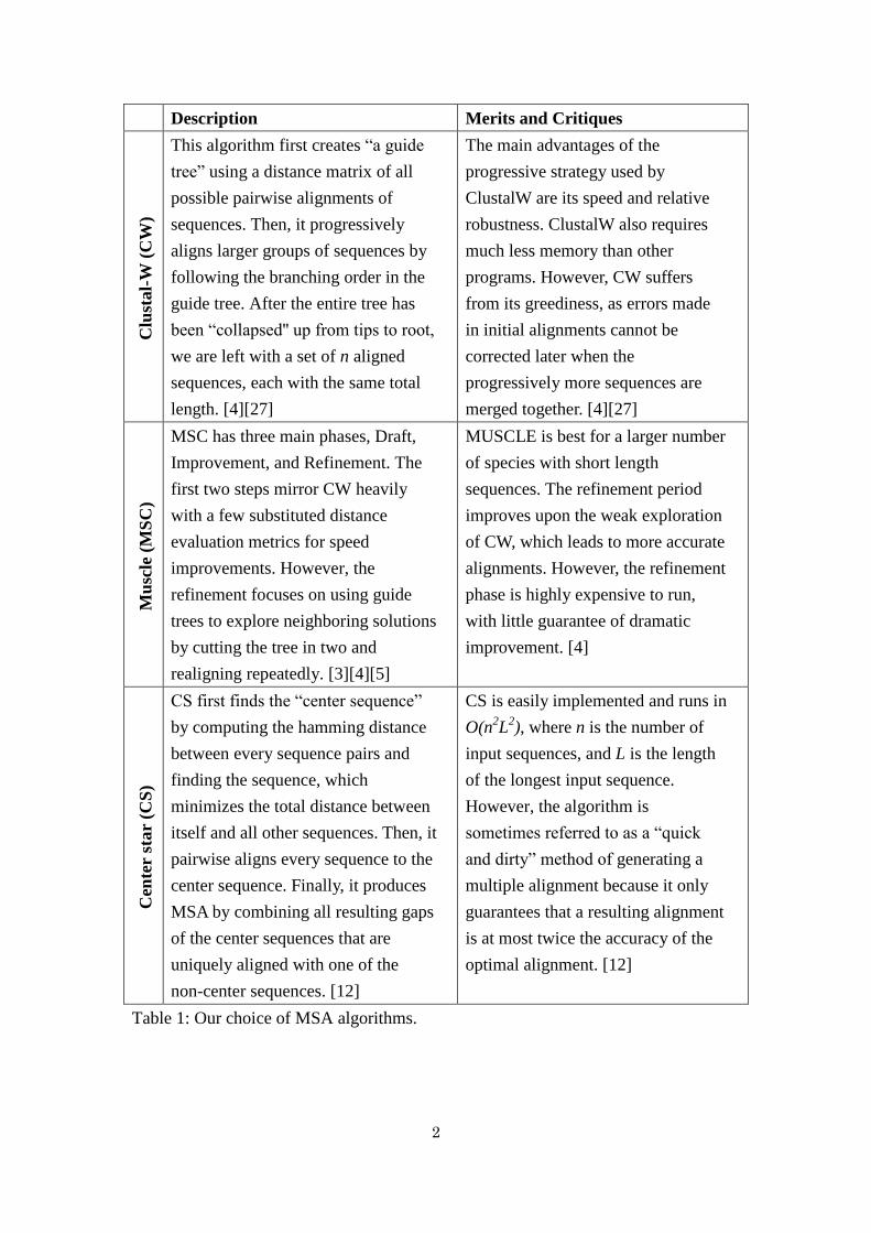
After conducting a literature review and determining which types of algorithms

were most frequently utilized, we decided to implement three MSA algorithms

(Table 1) and six phylogenetic reconstruction algorithms (Table 2a, 2b). In total, we

have 18 possible phylogenetic reconstruction methods, given our three sequence

aligners and our six tree reconstructors. Because these algorithms are so commonly

applied, state-of-the-art implementations for each exist. We acknowledge our

programs lack the nuance and optimizations found in these refined versions.

However, we argue that results derived from our implementations reflect basic

advantages and disadvantages that underlie each method.

2

Description Merits and Critiques

Clu

stal-

W (

CW

) This algorithm first creates “a guide

tree” using a distance matrix of all

possible pairwise alignments of

sequences. Then, it progressively

aligns larger groups of sequences by

following the branching order in the

guide tree. After the entire tree has

been “collapsed'' up from tips to root,

we are left with a set of n aligned

sequences, each with the same total

length. [4][27]

The main advantages of the

progressive strategy used by

ClustalW are its speed and relative

robustness. ClustalW also requires

much less memory than other

programs. However, CW suffers

from its greediness, as errors made

in initial alignments cannot be

corrected later when the

progressively more sequences are

merged together. [4][27]

Mu

scle

(M

SC

)

MSC has three main phases, Draft,

Improvement, and Refinement. The

first two steps mirror CW heavily

with a few substituted distance

evaluation metrics for speed

improvements. However, the

refinement focuses on using guide

trees to explore neighboring solutions

by cutting the tree in two and

realigning repeatedly. [3][4][5]

MUSCLE is best for a larger number

of species with short length

sequences. The refinement period

improves upon the weak exploration

of CW, which leads to more accurate

alignments. However, the refinement

phase is highly expensive to run,

with little guarantee of dramatic

improvement. [4]

Cen

ter

star

(CS

)

CS first finds the “center sequence”

by computing the hamming distance

between every sequence pairs and

finding the sequence, which

minimizes the total distance between

itself and all other sequences. Then, it

pairwise aligns every sequence to the

center sequence. Finally, it produces

MSA by combining all resulting gaps

of the center sequences that are

uniquely aligned with one of the

non-center sequences. [12]

CS is easily implemented and runs in

O(n2L

2), where n is the number of

input sequences, and L is the length

of the longest input sequence.

However, the algorithm is

sometimes referred to as a “quick

and dirty” method of generating a

multiple alignment because it only

guarantees that a resulting alignment

is at most twice the accuracy of the

optimal alignment. [12]

Table 1: Our choice of MSA algorithms.

3

Desription Merits and Critiques

Nei

gh

bor

Join

ing (

NJ)

Neighbor joining is a simple process

wherein a method of measurement is used to

evaluate the distance between sequences,

building the tree greedily with closest

sequences being conglomerated with one

another, and resolving later sequences after

treating the combined sections as a unified

sequence for the purpose of reevaluating

distances [21].

NJ is computationally efficient

since it only makes local

decisions during tree building. It

works well with a large set of

sequences [25]. Aside from its

greedy nature, it can obscure

ambiguities in data since it only

produces one tree.

Maxim

um

Lik

elih

ood

The core concept of ML is to find a

phylogenetic tree that has the highest

probability (likelihood) of a given tree

yielding the observed outcome [8]. The

likelihood of a tree is calculated as the

product of the likelihood values of all

evolutionary transitions inferred by the tree

structure. To find a tree with the highest

likelihood, we first start by maximizing the

likelihood of a topology1. By iteratively

optimizing the length of all branches within

in a topology, we can obtain the maximum

likelihood value of the topology. Using one

of the two topology-searching methods (see

the next section), we can then compare the

maximum likelihood values of topologies to

find a tree structure with the highest

likelihood [8].

While ML might produce more

accurate trees when compared to

other reconstruction methods, it

is computationally costly, mainly

due to the likelihood calculations

in the branch optimization

process. ML makes several

assumptions about evolution in

order to make likelihood

calculation simpler. This makes

it harder to account for

phenomena, such as insertion or

deletion mutation. In this project,

we resolve this problem by

assigning an imaginary

nucleotide for gaps [8][7]

Table 2a: Our Choice of reconstruction algorithms.

Tree searching methods

ML and MP fall into a greater class of tree “scoring” algorithms. Scoring algorithms

define an objective scoring function, and the user can utilize a variety of algorithms to

search through tree space. In this study, we implemented two types of tree searching

algorithms. The first approach is a heuristic approach that begins with a tree that

contains just two randomly chosen species. The final tree is progressively built up

1 Note that, with different branch length assignments, one topology can represent multiple different

tree structures.

4

Desription Merits and Critiques

Maxim

um

Pars

imon

y (

MP

) “The maximization of parsimony” or

preferring the simplest of otherwise equally

adequate theories is the guiding principle in

MP. With the assumption that evolution is

inherently a parsimonious process,

Maximum Parsimony values phylogenetic

trees where the least evolution is required to

group taxa together [9]. The objective

function we attempt to minimize is tree

“length”. Tree length refers to the minimum

number of mutations required to explain a

given topology. To determine the length of a

given tree, Fitch’s Algorithm [10] is used.

We use one of the two topology-search

methods to find the most parsimonious tree.

Because mutations are rare, the

tree of “minimal evolution” is

likely a good approximation of

the actual evolutionary history of

a system. However, obviously,

evolution is not a completely

parsimonious process, though it

is assumed to be in Fitch’s

original method. In addition,

because Maximum Parsimony

uses heuristic methods in

searching tree space, obtaining

the most parsimonious tree is not

guaranteed.

Mark

ov C

hain

Mon

te C

arl

o (

MC

MC

)

MCMC is a widely used tree sampling

approach. It starts with a parameter space

and a randomly selected tree, proposes a

new tree parameters based on the current

tree, accepts or rejects this new proposal,

and repeats this process to create a

distribution of sampled trees. Using the

appropriate proposal and decision-making

algorithms, the later samples after a burn-in

period [15] will be similar to the true

distribution of trees. In our case, we use the

GLOBAL and LOCAL with a molecular

clock [15] for parameter proposal, and the

Metropolis-Hastings algorithm to decide

whether the proposed tree will be accepted.

Since MCMC depends on the

underlying likelihood model,

data sequences generated by the

best fitted model would likely

differ from genuine data

regarding composition of amino

acids, locations of stop codons,

and other biologically relevant

features [15]. Another problem

is its ability to correctly identify

the posterior probabilities of the

collection of highly probable

tree topologies. It is difficult for

a particular simulation to visit

new regions of parameter space

once it gets stuck in an old

region [15].

Table 2b: Our choice of reconstruction algorithms.

from this simpler tree by adding one species at a time [8]. The second approach

begins with a randomly constructed tree containing all n species, inserted arbitrarily,

and uses hill-climbing to arrive at a local optimum [28]. The former method runs

5

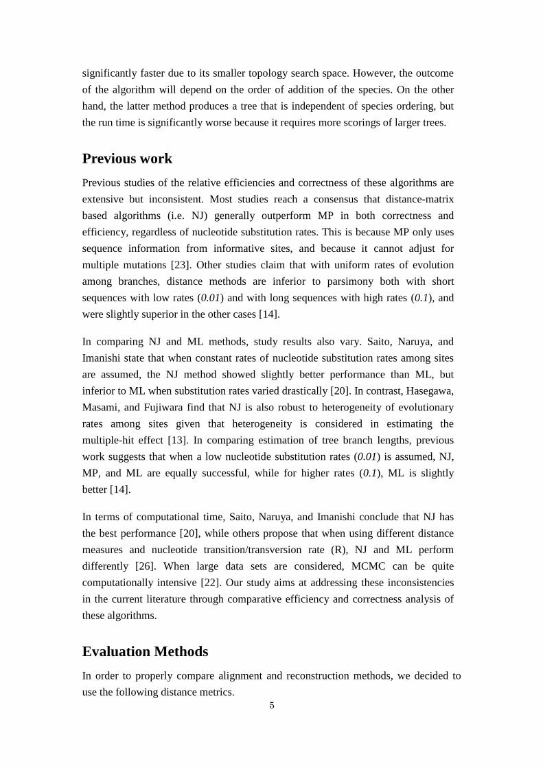
significantly faster due to its smaller topology search space. However, the outcome

of the algorithm will depend on the order of addition of the species. On the other

hand, the latter method produces a tree that is independent of species ordering, but

the run time is significantly worse because it requires more scorings of larger trees.

Previous work

Previous studies of the relative efficiencies and correctness of these algorithms are

extensive but inconsistent. Most studies reach a consensus that distance-matrix

based algorithms (i.e. NJ) generally outperform MP in both correctness and

efficiency, regardless of nucleotide substitution rates. This is because MP only uses

sequence information from informative sites, and because it cannot adjust for

multiple mutations [23]. Other studies claim that with uniform rates of evolution

among branches, distance methods are inferior to parsimony both with short

sequences with low rates (0.01) and with long sequences with high rates (0.1), and

were slightly superior in the other cases [14].

In comparing NJ and ML methods, study results also vary. Saito, Naruya, and

Imanishi state that when constant rates of nucleotide substitution rates among sites

are assumed, the NJ method showed slightly better performance than ML, but

inferior to ML when substitution rates varied drastically [20]. In contrast, Hasegawa,

Masami, and Fujiwara find that NJ is also robust to heterogeneity of evolutionary

rates among sites given that heterogeneity is considered in estimating the

multiple-hit effect [13]. In comparing estimation of tree branch lengths, previous

work suggests that when a low nucleotide substitution rates (0.01) is assumed, NJ,

MP, and ML are equally successful, while for higher rates (0.1), ML is slightly

better [14].

In terms of computational time, Saito, Naruya, and Imanishi conclude that NJ has

the best performance [20], while others propose that when using different distance

measures and nucleotide transition/transversion rate (R), NJ and ML perform

differently [26]. When large data sets are considered, MCMC can be quite

computationally intensive [22]. Our study aims at addressing these inconsistencies

in the current literature through comparative efficiency and correctness analysis of

these algorithms.

Evaluation Methods

In order to properly compare alignment and reconstruction methods, we decided to

use the following distance metrics.

6

Multiple Sequence Alignment comparison

In order to evaluate the qualities of the MSA algorithms, we calculated the total

distance of output multiple sequence alignments, using the following equation.

∑

Where L is the sequence length, α is the total number of non-matching indices

between two sequences, and β is the total number of non-dual-gap positions.

Quartet distance: Topological Metric

To compare the similarity of topologies numerically, we employ a “quartet” based

method, first proposed for this purpose by Estabrook, McMorris and Meacham [6]. A

quartet is a phylogenetic tree with only four species, divided by two internal nodes. To

compute the quartet distance between two phylogenetic trees, for each size four subset

of species, compare the corresponding quartet reductions in both trees. If the quartets

differ, add one to the total quartet distance. We implement Christiansen's method [2],

which computes quartet distance in O(n3) time.

Pairwise Path Distance: Branch Length Metric

Because quartet distance doesn't account for branch lengths and many of our tree

reconstruction algorithms produce weighted topologies, a secondary metric that

accounts for this additional information is required. First proposed by Williams and

Clifford [29], we utilize a version of pairwise pathlength distance similar to that

presented by Steel and Penny [24]. The focus of this comparison method is computing

all the pathlength between all pairs of species in a given phylogeny. To compute

pathlength between all pairs of nodes in a weighted graph, we use the Floyd-Warshall

algorithm [11].

More specifically, pairwise pathlength distance can be computed as follows. Given

two trees with associated branch lengths T1 and T2 each containing species

{S1,S2…Sn}, consider a fixed ordering of all possible species pairs <(S1,S2), (S1,S3) …

(Sn-1,Sn)>. Let 1 and 2

be the ordered pairwise pathlength distances between the

species specified in the ordering for T1 and T2. After normalizing these vectors such

that each of their largest components is equal to one, the pairwise path distance

between T1 and T2 is given by

𝑡ℎ 1 2 ‖ 1 − 2

‖2

7

Experiments

Comparing MSA Algorithms

In order to compare the performance of the three MSA algorithms (CW, MSC, CS),

we completed 14 runs for each alignment method for several numbers of sequences.

Using the evaluation method described previously, we calculated the total distance

of the resulting MSAs, and tested against each other in a student's T test.

Synthetic Data Experiments

We implemented a random data generator, which is capable of producing testing

examples <T, D>, where T is a randomly generated phylogenetic tree containing n

species, and D is a set of n sequences generated based on that synthetic tree. We can

use D as input to a total of 18 combinations of the 3 MSA algorithms and the 6

reconstruction algorithms. The output of these algorithms can be then be compared

to the true tree T and the tree using either of our distance metrics. Our random data

generator is governed by several input parameters, including the number of desired

species, the global mutation rate, and the starting sequence length. Because of our

limited computational resources, we were only able to execute a subset of the large

number of possible experiment. In total, we completed tree reconstructions from all

possible pairs of alignment and reconstruction algorithms in the Cartesian product:

{CW, CS}x{NJ, MP-Progressive, MP Hill-Climbing, ML Progressive, ML

Hill-Climbing, MCMC with likelihood}. We executed each of these 12

reconstruction methods on 14 randomly generated datasets with varying number of

species. The randomly generated datasets we used had a total number of species

between four and eight. Furthermore, we have a constant mutation parameter and

seed the mutation process with sequences of length 200. This gives us five distinct

datasets.

For each of the five datasets and 12 reconstruction methods, we evaluate the

performance of our algorithms over 14 trials. To evaluate their outputs, we compute

the average quartet distances and the average pairwise path distances, normalized to

[0,1]. Notably, one of our reconstruction methods, MP, does not produce meaningful

branch length predictions, so for any analysis associated with MPP or MPH, we

only use quartet distance. Furthermore, we measure the average runtime of each

algorithm in each scenario to quantify the computational efficiency of each

approach. Questions we address with experiment one include:

Do different algorithms perform significantly better or worse when there are

different numbers of species in the dataset?

8

Does algorithm runtime depend on problem difficulty, rather than problem

size?

Real Data Experiments

We have a dataset <T, D> where T is the commonly accepted phylogeny for 53

species (50 primates and 3 non-primates), and D is a set of the DNA sequences of

the mitochondrial cytochrome c oxidase subunit 1 (COX1) of those real species [18].

We decided to use the phylogeny of great apes because it is well-studied and

commonly agreed upon [18]. This makes the commonly accepted ape phylogeny a

great candidate for a “ground truth” to compare against. COX1 is a popular choice

for phylogenetic reconstruction because it is highly conserved due to its

involvement with aerobic respiration [17]. To produce varying numbers of species

in our input data, we can select random subsets of the 53 extant species for analysis.

14 test examples <T, D> with 5 species.

14 test examples <T, D> with 8 species.

Due to the computational intensity of the experiments, we were only able to run

Clustal-W alignments paired with our six reconstruction methods for each of these

28 datasets. Questions we address with experiment one include:

Do the random data results match the real data results?

Which algorithm performs fastest on the real data?

Which algorithm produces the most accurate tree on the real data?

Reconstruction Hypotheses

We hypothesize that the method with CS and NJ has the shortest average running

time on randomly generated data due to its algorithmic simplicity. We believe that

CW/ML and CW/MCMC will perform better than other methods in terms of the

accuracy of tree reconstruction on the random data because these algorithms make

fewer “binding” local decisions that might cause a build-up of errors.

Results

MSA Algorithms

Method comparison Real data Synthetic data

CW-CS -2.265 -0.666

CW-MSC -8.252 -2.016

CS-MSC -5.899 -1.309

Table 3: the result of the MSA experiment.

9

Each entry of Table 3 relates to the t-statistics of the former method being worse

than the latter using our evaluation described in the previous section. Hence in the

analysis of the real sequences of DNA every result was significant at p=.05 meaning

we get a hierarchy of CW>CS>MSC in terms of accuracy on real data, with respect

to our test statistic. However on the much shorter synthetic sequences of 1/8 length

the real data we only see significance at the same level in the CW-MSC comparison

Synthetic Data Experiments

In terms of the pairwise distance metric, Figure 1 illustrates the accuracy of our tree

outputs in terms of pairwise distance. Notably, NJ and ML Progressive consistently

did better than other reconstruction algorithms. On the other hand, the trees

produced by the MCMC method did significantly worse than trees produced by any

other reconstruction method. Choice of MSA algorithms did not have a visible

effect on the accuracy of a resulting tree.

The result for the quartet distance analysis is represented in Figure 2. Similarly

reconstruction with NJ, MP Progressive, and ML Progressive methods outperformed

other methods. Again, choice of MSA algorithms did not have a visible effect on the

accuracy of a resulting tree.

Figure 1: The result of pairwise pathlength distance analysis on all combinations of

MSA and reconstruction algorithms with 8 synthetic species.

10

Figure 2: The result of quartet distance analysis on all combinations of MSA and

reconstruction algorithms with 8 synthetic species. The red dotted line represents the

distance between a randomly guessed tree and the original tree.

Real Data Experiments

ML with the hill-climb search performed relatively better on the real data than on

the synthetic data, in terms of both distance metrics (Figure 3). The performance of

other algorithms remained similar.

Figure 3: The result of the pairwise pathlength and quartet distance analysis on the

trees reconstructed from the DNA sequences of randomly chosen 8 primate species.

11

Running Time Evaluation

Runtime analysis of both synthetic and real data (Figure 4) suggests the following:

NJ gave the fastest performance.

ML performed worse than Maximum Parsimony.

MCMC performed slower than ML for smaller synthetic data sets, and faster

than ML hill-climbing for bigger synthetic data sets.

These results are similar when using Center Star and MUSCLE alignment

algorithms.

Figure 4: Runtime comparison of reconstruction algorithms on synthetic (right) and

real (left) datasets using CW as a MSA algorithm.

Discussion

Tree Accuracy

In terms of pairwise distance metric, ML Progressive outperformed ML Hill-climb.

The only difference between the two reconstruction algorithms was their topology

searching method: progressive vs. hill-climb approach. The difference in

performance between these two algorithms can be explained as follows. The

downside of the progressive approach is that it makes local decisions when

searching through the space of possible topologies, and thus, a resulting tree

topology can sometimes be unreliable. However, this does not have a big impact

when trees are evaluated on pairwise distance, because it only measures the

distances between pairs of leaf nodes; pairwise distance does not account for the

position of a node within a tree. On the other hand, the hill-climb approach can

sometimes get caught in a local optimum. In our case, it is likely that the downside

of the hill-climb approach had a larger impact on resulting trees.

12

For quartet distance metric, Maximum Parsimony also achieved results with equally

high accuracies as NJ and ML methods. This is in agreement with [14], which

suggests that under low nucleotide substitution rates, NJ, MP, and ML should be

equally successful. Hill-climbing approaches performed significantly worse than

progressive approaches in terms of quartet distance metric. Again, this is likely due

to the fact that hill-climbing approaches can sometimes only find the local optimal

topology rather than the true global optimum.

NJ produced accurate results in our study for both pairwise distance and quartet

distance. This was in accordance with [20], which suggested that NJ performs

slightly better than ML methods under constant nucleotide substitution rates.

MCMC performed significantly worse than other reconstruction algorithms in terms

of both quartet and pairwise distance metrics. This is likely because we did not run

the algorithm long enough to find a reasonable global optimum. In order to find

trees close to the global optimum in our sample space, the suggested number of

iterations was 2000 [15]. Due to the time constraints in our project, we only ran 200

iterations.

Figure5: Pairwise pathlength distance of several methods over

varying numbers of species.

In Figure 5, we compare the correctness of tree output of various algorithms when

problems increase in size. Notably MCMC becomes increasingly less accurate when

the number of species increases. This is likely a reflection of the fact that tree space

is less able to be explored in a fixed 200 iterations when more species are added.

Furthermore, using likelihood and hill climbing appears to become less correct and

more variable for larger problems as well. Because the objective function increases

significantly in complexity as the number of species increases, it's likely the case

that getting caught in local optima becomes increasingly common. On the other

hand, NJ and MLP perform relatively consistently, indicating their potential

accuracy on larger datasets.

13

Running Time

The expected efficiency of NJ is consistent with our experimental results. ML, on

the other hand, is considered computationally costly with progressive topology

(O(mn6)) and with the hill-climb approach (O(kmn

5)) due to the branch optimization

process. MCMC, which uses ML's likelihood calculations, is also computationally

expensive. These theoretical observations also agree with our experimental results.

MP had a performance speed that fell in between NJ and ML, which also fits our

expectation.

Conclusion

Based on our experiments with both synthetic and real data, and our analysis of both

run-time efficiencies and the accuracies of our algorithms, we conclude that for data

sets with similar properties to those of our data (i.e. short sequences, low and

constant nucleotide substitution rates), Neighbor Joining should be used in order to

achieve the best efficiency and accurate results. Maximum Likelihood with

progressive tree search creates equally accurate trees, but is far more

computationally expensive.

However, due to the complexity of the real-world data sets and their varying

characteristics, algorithms should be carefully chosen in order to obtain accurate

results. Based on our results, we cannot determine the total superiority of a specific

reconstruction method. In addition, there is no guarantee that the details of our

implementation match those in the literature we surveyed. Nonetheless, our study

provides a comparative approach that future research alike can undertake.

In the future, we would like to examine more types of synthetic data (perhaps

varying mutation characteristics) and optimize our implementations in accordance

with modern advancements to get a better sense of the current state of the field.

References

[1] D. Baum. Reading a phlogenetic tree: The meaning of monophletic groups.

Nature Edcation, 1, 2008.

[2] C. Christiansen, T. Mailund, C. N. Pedersen, and M. Randers. Computing the

quartet distance between trees of arbitrary degree. Springer, 2005.

[3] R. C. Edgar. Muscle: multiple sequence alignment with high accuracy and high

throughput. Nucleic acids research, 32(5):1792–1797, 2004.

14

[4] R. C. Edgar and S. Batzoglou. Multiple sequence alignment. Current opinion in

structural biology, 16(3):368–373, 2006.

[5] R. C. Edgar and K. Sjolander. A comparison of scoring functions for protein

sequence profile alignment. Bioinformatics, 20(8):1301–1308, 2004.

[6] G. F. Estabrook, F. McMorris, and C. A. Meacham. Comparison of undirected

phylogenetic trees based on subtrees of four evolutionary units. Systematic Biology,

34(2):193–200, 1985.

[7] S. Evans and T. Warnow. Phylogenetic analyses of

alignments with gaps.

[8] J. Felsenstein. Evolutionary trees from dna sequences: a maximum likelihood

approach. Journal of molecular evolution, 17(6):368–376, 1981.

[9] W. M. Fitch. Toward defining the course of evolution: minimum change for a

specific tree topology. Systematic Biology, 20(4):406–416, 1971.

[10] W. M. Fitch, E. Margoliash, et al. Construction of phylogenetic trees. Science,

155(760):279–284, 1967.

[11] R. W. Floyd. Algorithm 97: shortest path. Communications of the ACM,

5(6):345, 1962.

[12] D. Gusfield. Efficient methods for multiple sequence alignment with guaranteed

error bounds. Bulletin of mathematical biology, 55(1):141–154, 1993.

[13] M. Hasegawa and M. Fujiwara. Relative efficiencies of the maximum

likelihood, maximum parsimony, and neighbor-joining methods for estimating

protein phylogeny. Molecular phylogenetics and evolution, 2(1):1–5, 1993.

[14] M. K. Kuhner and J. Felsenstein. A simulation comparison of phylogeny

algorithms under equal and unequal evolutionary rates. Molecular Biology and

Evolution, 11(3):459–468, 1994.

[15] B. Larget and D. L. Simon. Markov chain monte carlo algorithms for the

bayesian analysis of phylogenetic trees. Molecular Biology and Evolution, 16:750–

759, 1999.

[16] W. Li, Z. Shi, M. Yu, W. Ren, C. Smith, J. H. Epstein, H. Wang, G. Crameri, Z.

Hu, H. Zhang, et al. Bats are natural reservoirs of sars-like coronaviruses. Science,

310(5748):676–679, 2005.

[17] F. F. Nord and D. E. Green. Electron transport and oxidative phosphorylation.

Advances in Enzymol-ogy and Related Areas of Molecular Biology, 21:73, 2009.

[18] P. Perelman, W. E. Johnson, C. Roos, H. N. Seuanez, ´J. E. Horvath, M. A.

Moreira, B. Kessing, J. Pontius,M. Roelke, Y. Rumpler, et al. A molecular

phylogeny of living primates. PLoS genetics, 7(3):e1001342,2011.

15

[19] S. Pillai, B. Good, S. Pond, W. J.K., M. Strain, D. Richman, and S. D.M.

Semen-specific genetic characteristics of humans immunodeficiency virus type 1

env. Journal of Virology, 79:1734–1742, 2005.

[20] N. Saitou and T. Imanishi. Relative efficiencies of the fitch argoliash, maximum

parsimony, maximum likelihood, minimum evolution, and neighbor joining

methods of phylogenetic tree construction in obtaining the correct tree. Mol. Biol.

Evol, 6(5):514–525,1989.

[21] N. Saitou and M. Nei. The neighbor-joining method: a new method for

reconstructing phylogenetic trees. Mol. Biol. Evol, 4(4):406–425, 1987.

[22] L. Salter. Algorithms for phylogenetic tree reconstruction. In Proceeding of the

International Conference on Mathematics and Engineering Techniques in Medicine

and Biological Sciences, volume 2, pages 459–465. Citeseer, 2000.

[23] J. Sourdis and M. Nei. Relative efficiencies of the maximum parsimony and

distance-matrix methods in obtaining the correct phylogenetic tree. Molecular

biology and evolution, 5(3):298–311, 1988.

[24] M. A. Steel and D. Penny. Distributions of tree comparison metricssome new

results. Systematic Biology,

42(2):126–141, 1993.

[25] K. Tamura, M. Nei, and S. Kumar. Prospects for inferring very large

phylogenies by using the neighbor joining method. Proceedings of the National

Academy of Sciences of the United States of America, 101(30):11030–11035, 2004.

[26] Y. Tateno, N. Takezaki, and M. Nei. Relative efficiencies of the maximum

likelihood, neighbor joining, and maximum parsimony methods when substitution

rate varies with site. Molecular Biology and Evolution, 11(2):261–277, 1994.

[27] J. D. Thompson, D. G. Higgins, and T. J. Gibson. Clustal w: improving the

sensitivity of progressive multiple sequence alignment through sequence weighting,

position-specific gap penalties and weight matrix choice. Nucleic acids research,

22(22):4673–4680, 1994.

[28] M. S. Waterman and T. F. Smith. On the similarity of dendrograms. Journal of

Theoretical Biology, 73(4):789–800, 1978.

[29] W. Williams and H. Clifford. On the comparison of two classifications of the

same set of elements. Taxon, pages 519–522, 1971.