Hirzi Luqman 1st September 2010

1

A Phylogenetic Approach to Comparative Linguistics:

a Test Study using the Languages of Borneo

Abstract

The conceptual parallels between linguistic and biological evolution are striking; languages, like genes are subject to mutation, replication, inheritance and selection. In this study, we explore the possibility of applying phylogenetic techniques established in biology to linguistic data. Three common phylogenetic reconstruction methods are tested: (1) distance-based network reconstruction, (2) maximum parsimony and (3) Bayesian inference. We use network analysis as a preliminary test to inspect degree of horizontal transmission prior to the use of the other methods. We test each method for applicability and accuracy, and compare their results with those from traditional classification. We find that the maximum parsimony and Bayesian inference methods are both very powerful and accurate in their phylogeny reconstruction. The maximum parsimony method recovered 8 out of a possible 13 clades identically, while the Bayesian inference recovered 7 out of 13. This match improved when we considered only fully resolved clades for the traditional classification, with maximum parsimony scoring 8 out of 9 possible matches, and Bayesian 7 out of 9 matches.

Introduction

“The formation of different languages and of distinct species, and the proofs that both have been developed through a gradual process, are curiously parallel... We find in distinct languages striking homologies due to community of descent, and analogies due to a similar process of formation... We see variability in every tongue, and new words are continually cropping up; but as there is a limit to the powers of the memory, single words, like whole languages, gradually become extinct ... To these more important causes of the survival of certain words, mere novelty and fashion may be added; for there is in the mind of man a strong love for slight changes in all things. The survival or preservation of certain favoured words in the struggle for existence is natural selection” (Darwin, 1871). The conceptual parallels between biological evolution and linguistic evolution have been noticed since the advent of modern (Darwinian) evolutionary theory itself, nearly a century and a half ago. Languages, like species, are a product of change and evolution. They chronicle their evolutionary history in a similar way to how genes record our own evolutionary past. Just as genes are replicated and inherited, so too are the sounds, grammar and lexicon of a language learnt and passed on. Just as mutations and natural selection lead to variable populations and species, so too do shifts, innovation and societal trends lead to

different dialects and languages. And just as phylogenetic inference may be muddied by horizontal transmission, so too may borrowing and imposition cloud true linguistic relations. These fundamental similarities in biological and language evolution are obvious, but do they imply that tools and methods developed in one field are truly transferable to the other? Or are they merely clever and coincidental analogies paraded by those attempting to Darwinize language and culture?

Recently, there has been a flux of studies applying phylogenetic methods to non-biological entities, particularly languages (see Gray & Jordan 2000; Holden 2002; Rexová et al 2002, 2006; Forster & Troth 2003; Gray & Atkinson 2003; Nakhleh et al 2005; Holden & Gray 2006; Atkinson et al 2008; Gray et al 2009; Kitchen et al 2009). This employment of computational statistics to infer evolutionary relatedness is standard in its home field of biology, but relatively new to historical linguistics. Somewhat surprising, given that similarities in their two respective processes of evolutionary change have been noted as far back as Darwin; but the conservativeness in applying such (phylogenetic) approaches to linguistic data is justifiable. According to critics (Gould 1987, 1991; Bateman et al 1990; Moore 1994; Belwood 1996; Borgerhoff Mulder 2001; Holden & Shennan 2005; Temkin & Eldredge 2007), phylogenetic methods based on

2

tree-building algorithms may not be truly applicable to linguistic data. In particular, it is frequently argued that horizontal transmission of traits is relatively common in language evolution and that this violates the assumptions of traditional (tree-building) phylogenetic methods (Gould 1987; Terrell 1998; Moore 1994; Terrell et al 2001). Instead of a tree model of languages, a network model or wave model may be more appropriate. This is a valid argument and has to be addressed before any further advance on cross method application can be made. (1) Conceptually, a general theory of evolutionary change, one that encompasses biological evolution, language evolution, cultural evolution and any other phenomena indicative of evolutionary change, is needed (Croft 2008). Several models attempting to do so have been developed, most notably those by Dawkins (1989, 1982), and Hull (1988, 2001). The key features to these generalized theories of evolution are that they generalize and incorporate the three most fundamental processes; that of (a) cumulative and iterative replication (leading to inheritance), (b) the generation of variation during replication, and (c) the selection of variants via some selective mechanism. The encompassing quality of such a model serves to clarify and standardize the analogies present in the constituent fields, allowing for a clearer framework for comparison and interdisciplinary method application. (2) Analytically, the degree of horizontal transfer should be determined using network visualisation tools, such as SplitsTree (Huson & Byrant 2006), which do not assume a tree-like model of evolution. Only on the condition of no significant reticulation should further phylogenetic methods (based on tree-building) be considered.

Following these two criteria should support in determining both the applicability and validity of using phylogenetic methods on linguistic data. In this study, we will be testing such an approach on a subset of languages from Borneo. Given that no significant reticulation is seen, we will be testing the applicability and accuracy of three common phylogenetic methods on our linguistic data set: 1) Split Decomposition and Neighbor Net distance-based network algorithms, 2) weighted and unweighted Maximum Parsimony and 3) Bayesian Inference. The accuracy of the methods will be tested by comparing their results with those established from traditional methods.

There do of course exist some other differences between biological and linguistic evolution; for example, languages change much faster than genes and selection of favoured variants is determined by societal trends rather than fitness difference among alleles; however none of these differences are fundamental to a general theory of evolutionary change (e.g. of Dawkins 1982, 1989; Hull 1988, 2001). For instance, the former merely entails a restriction of (phylogenetic) inferences to more recent timeframes, while the latter, a superficial difference function-wise.

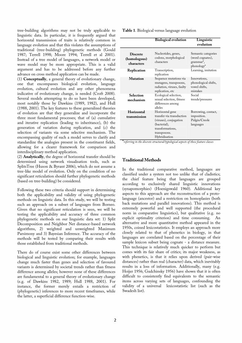
Table 1. Biological versus language evolution

Biological evolution Linguistic evolution

Discrete

(homologous) characters

Nucleotides, genes, codons, morphological characters

Semantic categories (word cognates), grammar*, phonology*

Replication Transcription, replication

Learning, imitation

Mutation Sequence mutations via mutagens, transposons, radiation, viruses, faulty replication, etc

Innovations, phonological shifts, vowel shifts, mistakes

Selection mechanism

Ecological selection, sexual selection, fitness differences among alleles

Social trends/pressures

Horizontal transmission

Horizontal gene transfer via transduction (viruses), conjugation (bacterial), transformations, transposons. Hybridisation

Borrowing, contact, imposition. Pidgin/Creole languages

*referring to the discrete structural/typological aspects of these feature classes

Traditional Methods

In the traditional comparative method, languages are classified under a system not too unlike that of cladistics; the chief feature being that languages are grouped according to exclusively shared linguistic innovations (synapomorphies) (Hoenigswald 1960). Additional key aspects to this approach are the reconstruction of a proto-language (ancestor) and a restriction on homoplasies (both back mutations and parallel innovations). This method is extremely powerful and well supported (the procedural norm in comparative linguistics), but qualitative (e.g. no explicit optimality criterion) and time consuming. An alternative and more quantitative method appeared in the 1950s, coined lexicostatistics. It employs an approach more closely related to that of phenetics in biology, in that languages are correlated based on the percentage of their sample lexicon subset being cognate - a distance measure. This technique is relatively much quicker to perform but comes with its fair share of critics; its major weakness, as with phenetics, is that it relies upon derived (pair-wise distances) rather than real (character) data, which inevitably results in a loss of information. Additionally, many (e.g. Hoijer 1956; Gudchinsky 1956) have shown that it is often difficult to consistently find equivalents to the semantic items across varying sets of languages, confounding the validity of a universal lexicostatistic list (such as the Swadesh list).

3

Methods & Materials

In this study, we attempt to merge the fundamental concepts of the traditional comparative method with the quantitative character (but not procedure) of lexicostatistics, primarily via the methods of maximum parsimony and Bayesian inference (which are character-based and quantitative). We seek to find out how applicable and accurate such methods can be when applied to an example linguistic data set.

1. Characters

Our study uses lexical characters to characterise linguistic information. Lexical characters here are represented by word cognates (literally blood relatives –Latin). These are words that demonstrably, via systematic sound correspondences, historical records and the Comparative Method derive from a common ancestor, and thus represent homologous characters akin to those in biology. The use of lexical characters has been well supported and established in comparative linguistics, and given that we adhere firmly to the criterion of using only basic vocabulary, is well suited in determining relationships that are genetic rather than due to chance or contact and borrowing. As they are relatively fast changing (Greenhill et al 2010), they also represent the most suitable unit of linguistic change for our dataset; which is one of fairly close relation (Western Malayo-Polynesian subfamily). Two other types of characters, phonological and morphological (grammatical) were also considered, but later discarded due to lack of data1 for our set of languages. Ideally they should be included; they represent different and additional aspects of language change and can thus provide additional resolution and information at different time depths than can lexical characters, but the lack of available data and time precluded this measure.

2. Cognate Judgment

As cognates represent the characters of our data set, their correct judgement is fundamental to acquiring good results. The process of cognate judgment is thus not a trivial one. Judgement can be subjective and dependent on good historical records; for cognates do not necessarily look similar2. Consequently, cognate judgement was left to the linguists – we opted to source data only from language databases with present and good cognate judgements.

1 The World Atlas of Language Structures (WALS), the most comprehensive

database for structural characters, unfortunately had incomplete data for many of

our subject languages and feature classes. 2 For example the English ‘wheel’ and Hindi ‘cakra’ are cognates even though

they appear entirely different; they are only identifiable as such due to good

historical records.

3. Data Set & Source

For our study, we selected a subset of 26 languages from Borneo3. Approximately 150 languages are currently spoken in Borneo (Lewis 2009)4; but the lack of research and sufficient data in many (the remaining number) prohibited (their) inclusion into our analysis. Additionally, a language outgroup from the Formosan language family was included to facilitate tree/network rooting where applicable. A Formosan (Taiwanese) ancestry for Austronesian languages has been firmly established through linguistic evidence (Blust 1999), archaeological evidence (Belwood 1997) and genetic evidence (Trejaut et al 2005).

All language data was sourced from the Austronesian Basic Vocabulary Database (ABVD) (Greenhill et al 2008). This was selected as it is currently the most complete and comprehensive database for Austronesian languages, and includes the lexical and cognate data for 667 languages. For each language, the database lists 210 word items of basic vocabulary (see Wordlist in Appendix A2), along with their cognate judgements. We advise you to refer to their paper (Greenhill et al 2008, The Austronesian Basic Vocabulary Database: From Bioinformatics to Lexomics) for any inquires into data sources, collection methodology, cognate identification procedures, database content and structure.

4. Word list

The original 210 basic word list sourced from the ABVD was reduced to 64 words after careful consideration. After examining each language wordlist side by side, we found that a fair number of the words, for our collection of languages, were not fulfilling some fundamental and requisite criteria. We have listed these criteria below:

1. Words have to be items of basic vocabulary and thus ones least prone to replacement with loan words. E.g. body parts, close kinship terms, numbers and basic verbs.

2. Words should have a firm, distinct meaning. Plasticity and homonymy, given lack of consideration, may lead to false cognate judgements.

3. Words should have all synonym forms considered and present in database. Having only one representative word per semantic category (or less than in reality) may lead to false cognate judgements.

4. Words should be transferrable. In other words, its meaning should be conceptually present across all subject languages/cultures. For example, having ‘snow’ as a basic semantic item across localities/languages that lack such an entity is incorrect.

5. Words should occupy conceptually basic semantic categories, and not culturally/scientifically derived categories (similar to 1). For example, a local culture

3 See Appendix A1 for selected language list 4 See Appendix for full language list and map

4

may not necessarily recognize the scientifically derived distinctions between midges, flies and mosquitoes, and only have one term for all three, “small biting flying thing”, so having three separate semantic categories (words) for each of them would be misleading.

6. The word should belong to a distinct and absolute semantic category, rather than one situated on a relative and continuous scale (such as temperature, colour, size etc). This is because different cultures may perceive categories differently, and divide continuous scales at different resolutions. For example, blue and green are shades of the same colour in some Chinese cultures/languages (青, qīng – Mandarin) while perceived as different colours/words under the English language.

These criteria were put together in order to filter out words that may lead to false cognate judgements and consequently false historical inferences. It is true that reducing the number of words (characters) potentially reduces the accuracy and support of inferred topologies (Hillis 1998; Page & Holmes 1998; Scotland et al 2003; Scotland & Wortley 2006), but this is so only if the characters removed are good and representative of evolutionary history.

Quite a few of the words removed from the original 210 were those that failed criteria 2 and 3; i.e. words whose various forms and meanings were deemed inadequately researched/considered at the time of data sourcing5, and thus likely prone to false cognate judgements. This was a necessary step as the ABVD is still a relatively new and thus incomplete database, with entries still constantly being updated.

5. Coding

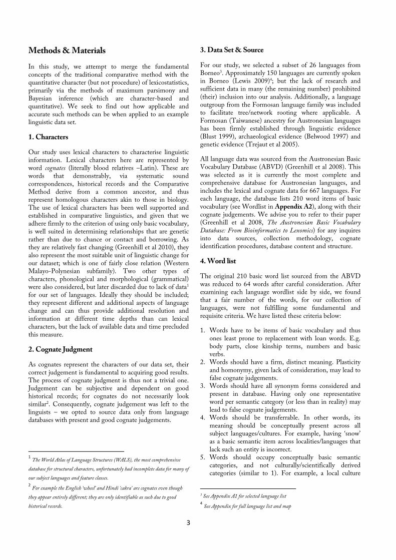
We code our lexical data similar to how we code any character data in biology; by allocating a unique number or symbol to each unique form present. An example of this process is shown below.

Table 2. Encoding methodology

‘hand’ Cognacy

(ABVD)

Cognacy

(renumbered)

Iranun lima 1 1

Melayu tangan 18 2

Singhi toŋan 18 2

Bintulu agem 20 4

This data representation is typically lossless with discrete and fixed character states (as with molecular data) but

5 Word synonyms, homonyms and various forms/meanings were cross referenced

with local dictionaries and speakers, for a measure of term completeness.

potentially lossy with continuous and variable ones; like morphological data and here, lexical data. For example, a lexical unit may change in a variety of ways:

• replacement with a loan; • replacement with a novel morpheme; • loss with no replacement; • semantic change or addition; • morphological change (e.g. suffixed, derived, reanalysed); • deconstruction into two or more separate derivatives; • unlinked changes (e.g. phonological change occurring with no simultaneous morphological or semantic change) • creation of homophones

Of the above, only absolute loss and gain/replacement events are typically represented encoded. The more partial and nuance changes are less easily captured by discrete character encoding, yet they are evolutionary informative. Consequently, their exclusion through coding does lead to loss of some valuable information.

It would be interesting to see how much of an effect this lossy encoding process has on our results, but at present, it is outside the scope of our study. We can only assume, like in many other lexicostatistic and morphological (biology) studies, that their affects are relatively minor compared to the stronger loss/gain events, and that their exclusion only has minimum bearing on the topology of inferred phylogenies.

Note: Ideally, we would want a coding system that manages to accommodate both the absolute loss/gain events with the more subtle, partial changes described above – but we found this too impractical and prohibitive to realize.6

6. Multistate vs. Binary

In our study, we code lexical character data in two ways: (1) Multistate and (2) Binary.

For (1), the character states are the various cognate forms; for (2) the character states indicate the presence or absence

6 *It is theoretically possible to construct a hierarchical and

characterstate-numerous multistate matrix to accommodate each and every different mechanism and degree of change. However, this was found to prohibitively complicated, impractical and resource intensive. For instance, you would likely end up with more than 64 character states per character (semantic category) to accommodate every different cognate form, morphology, change mechanism, etc – which is above the bit manipulation capacity of most (e.g. 32-bit, 64-bit) programmes and computers – and each character state transition would also have to be modelled (potentially) differently.

5

of a cognate form. Binary characters here are merely deconstructions of the more inclusive multistate characters (see Figure 1 for example).

There are several important differences between the two coding methods that need to be taken note off prior to analysis.

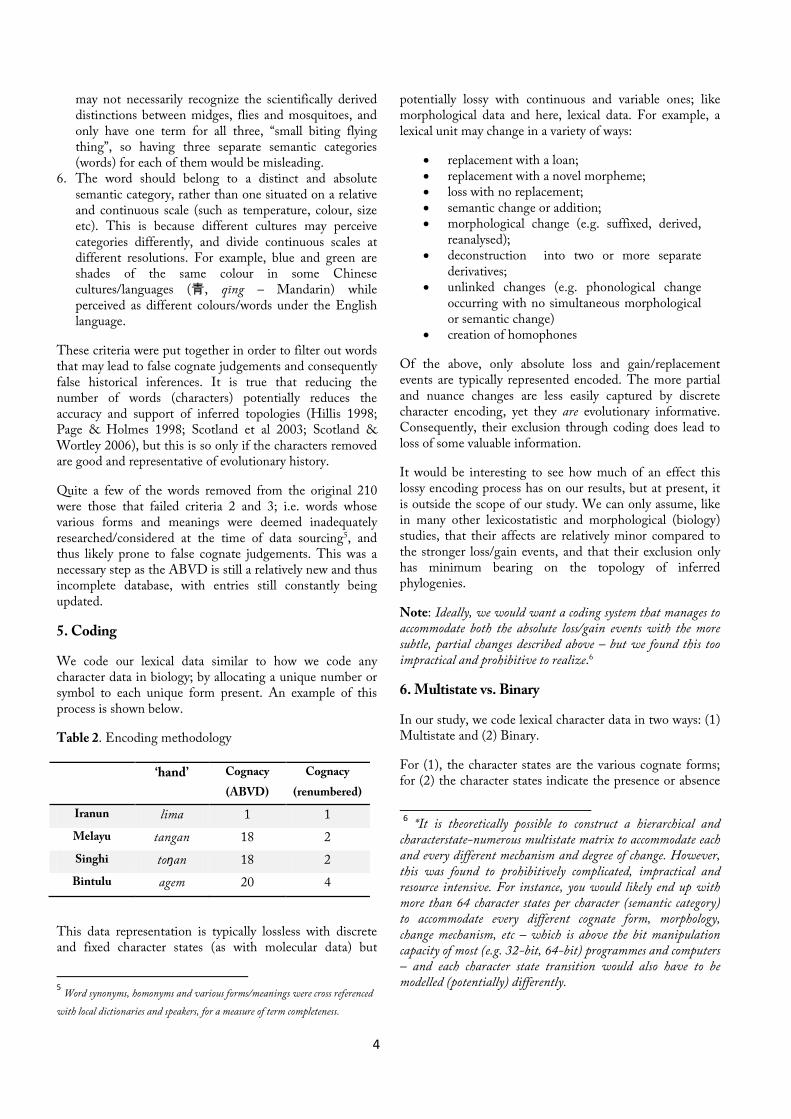
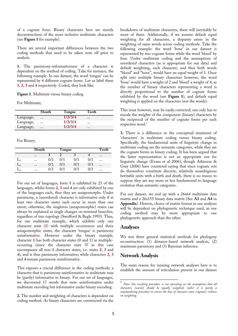
1. The parsimony-informativeness of a character is dependent on the method of coding. Take for instance, the following example. In our dataset, the word ‘tongue’ can be represented by 4 different cognate forms. Let us label them 1, 2, 3 and 4 respectively. Coded, they look like:

Figure 1. Multistate versus binary coding

For Multistate;

Mouth Tongue Teeth

Language1 ... 1/2/3/4 ... Language2 ... 1/2/3/4 ... Languagen ... 1/2/3/4 ...

For Binary;

Mouth Tongue Teeth

... 1 2 3 4 ... L1 ... 0/1 0/1 0/1 0/1 ... L2 ... 0/1 0/1 0/1 0/1 ... Ln ... 0/1 0/1 0/1 0/1 ...

For our set of languages, form 1 is exhibited by 23 of the languages, whilst forms 2, 3 and 4 are only exhibited by one of the languages each, thus they are autapomorphs. Under parsimony, a (unordered) character is informative only if at least two character states each occur in more than one taxon; otherwise, the singleton (autapomorphic) states can always be explained as single changes on terminal branches, regardless of tree topology (Swofford & Begle 1993). Thus, for our multistate example, which exhibits only one character state (1) with multiple occurrences and three autapomorphic states, the character ‘tongue’ is parsimony uninformative. However under the binary example, character 1 has both character states (0 and 1) as multiple-occurring (since the character state ‘0’ in this case encompasses all non-1 character states, i.e. states 2, 3 and 4), and is thus parsimony informative; while characters 2, 3 and 4 remain parsimony uninformative.

This exposes a crucial difference in the coding methods; a character that is parsimony uninformative in multistate may be (partly) informative in binary. For our set of languages, we discovered 17 words that were uninformative under multistate encoding but informative under binary encoding.

2. The number and weighting of characters is dependent on coding method. As binary characters are constructed via the

breakdown of multistate characters, there will inevitably be more of them. Additionally, if we assume default equal weighting for all characters, a disparity arises in the weighting of same words across coding methods. Take the following example: the word ‘bone’ in our dataset is represented by two cognate forms while the word ‘blood’ by four. Under multistate coding and the assumptions of unordered characters (as is appropriate for our data) and default weighting, each character, and thus both words “blood” and “bone”, would have an equal weight of 1. Once split into multiple binary characters however, the word ‘bone’ would have a weight of 2 and ‘blood’ a weight of 4; as the number of binary characters representing a word is directly proportional to the number of cognate forms exhibited by the word (see Figure 1), and default equal weighting is applied on the characters (not the words).

This issue however, may be easily corrected; one only has to rescale the weights of the component (binary) characters by the reciprocal of the number of cognate forms per each respective word.7

3. There is a difference in the conceptual treatment of ‘characters’ in multistate coding versus binary coding. Specifically, the fundamental units of linguistic change in multistate coding are the semantic categories, while they are the cognate forms in binary coding. It has been argued that the latter representation is not an appropriate one for linguistic change (Evans et al 2006); though Atkinson & Gray (2006) have countered saying that since cognate sets do themselves constitute discrete, relatively unambiguous heritable units with a birth and death, there is no reason to suppose they are any more or less fundamental to language evolution than semantic categories.

For our dataset, we end up with a 26x64 multistate data matrix and a 26x155 binary data matrix (See A3 and A4 in Appendix). Hereon, choice of matrix format in our analyses will be dependent on phylogenetic technique used, as one coding method may be more appropriate to one phylogenetic approach than the other.

Analyses

We test three general statistical methods for phylogeny reconstruction: (1) distance-based network analysis, (2) maximum parsimony and (3) Bayesian inference.

Network Analysis

The main reason for running network analyses here is to establish the amount of reticulation present in our dataset

7 Note: this rescaling procedure is not operating on the assumption that all

characters (words) should be equally weighted; rather it is purely a standardizing procedure to correct the bias of character-state (cognate) richness on weighting.

6

preliminary to further tree-based phylogenetic approaches. Only on condition of little or insignificant reticulation will these latter techniques be considered. A secondary reason is for the reconstructed phylogeny.

For network visualization, we employ two separate distance-based algorithms: (1) Neighbor-Net and (2) Split Decomposition. Both algorithms were run under SplitsTree4 V4.11.3 (Huson & Byrant 2006).

The Split Decomposition method canonically decomposes a distance matrix into simple components based on weighted splits (bipartitions of the taxa set), subsequently representing these splits in a splits graph. Neighbor-Net is similar in that it also constructs and visually represents weighted splits, but differs in producing circular (rather than weakly compatible) splits and in using an agglomeration method based on the Neighbour-Joining (NJ) algorithm.

We use our data encoded in the multistate format for the network analyses. We do so in light of (a) there is no difference in informativeness between coding methods as described in (6.1) above, as these distance-based phenetic approaches operate outside the premise of cladistics. More specifically, autapomorphic characters here are informative as they are capable of defining splits; (b) for distance-based approaches, the multistate format is a more accurate representation of the data. This reason (b) is justified through the observation that binary encoding of data introduces an error whereby the absence of a character is treated as character identity (zero-distance), which skews distance measures. To highlight this problem, we observe the following example:

We have a character X, with character states 1, 2 and 3. Coded, it looks like:

Multistate Binary

X X 1 2 3 L1 1 L1 1 0 0 L2 1 L2 1 0 0 L3 2 L3 0 1 0 L4 3 L4 0 0 1

A transformation of the multistate character matrix to a distance one gives (assuming equal transition probabilities and unordered characters):

L1 L2 L3 L4 L1 0 0 1 1 L2 0 0 1 1 L3 1 1 0 1 L4 1 1 1 0

While a transformation from the binary character matrix to a distance one gives8 (with same assumptions):

L1 L2 L3 L4 L1 0 0 2 2 L2 0 0 2 2 L3 2 2 0 3 L4 2 2 3 0

We see here how the treatment of absence as identity skews the distance matrix under binary coding, thus giving us justified preference for the use of the multistate format.

Programme settings used for the network analyses are as follows: distance: UncorrectedP; draw: EqualAngle; network: NeighborNet/SplitDecomposition. A bootstrap analysis of 10,000 runs followed the network constructions to estimate support of the splits.

Results

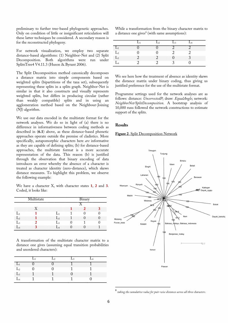
Figure 2. Split Decomposition Network

8 taking the cumulative value for pair-wise distances across all three characters.

7

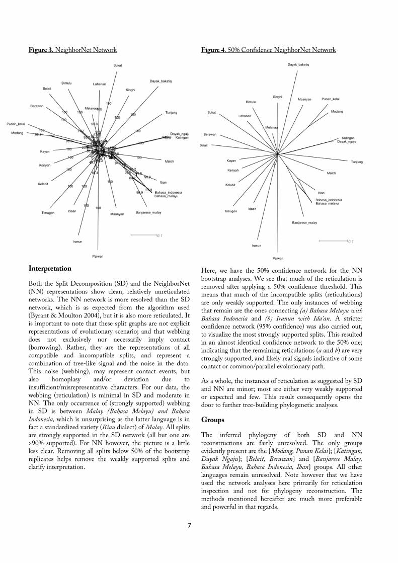
Figure 3. NeighborNet Network

Interpretation

Both the Split Decomposition (SD) and the NeighborNet (NN) representations show clean, relatively unreticulated networks. The NN network is more resolved than the SD network, which is as expected from the algorithm used (Byrant & Moulton 2004), but it is also more reticulated. It is important to note that these split graphs are not explicit representations of evolutionary scenario; and that webbing does not exclusively nor necessarily imply contact (borrowing). Rather, they are the representations of all compatible and incompatible splits, and represent a combination of tree-like signal and the noise in the data. This noise (webbing), may represent contact events, but also homoplasy and/or deviation due to insufficient/misrepresentative characters. For our data, the webbing (reticulation) is minimal in SD and moderate in NN. The only occurrence of (strongly supported) webbing in SD is between Malay (Bahasa Melayu) and Bahasa Indonesia, which is unsurprising as the latter language is in fact a standardized variety (Riau dialect) of Malay. All splits are strongly supported in the SD network (all but one are >90% supported). For NN however, the picture is a little less clear. Removing all splits below 50% of the bootstrap replicates helps remove the weakly supported splits and clarify interpretation.

Figure 4. 50% Confidence NeighborNet Network

Here, we have the 50% confidence network for the NN bootstrap analyses. We see that much of the reticulation is removed after applying a 50% confidence threshold. This means that much of the incompatible splits (reticulations) are only weakly supported. The only instances of webbing that remain are the ones connecting (a) Bahasa Melayu with Bahasa Indonesia and (b) Iranun with Ida’an. A stricter confidence network (95% confidence) was also carried out, to visualize the most strongly supported splits. This resulted in an almost identical confidence network to the 50% one; indicating that the remaining reticulations (a and b) are very strongly supported, and likely real signals indicative of some contact or common/parallel evolutionary path.

As a whole, the instances of reticulation as suggested by SD and NN are minor; most are either very weakly supported or expected and few. This result consequently opens the door to further tree-building phylogenetic analyses.

Groups

The inferred phylogeny of both SD and NN reconstructions are fairly unresolved. The only groups evidently present are the {Modang, Punan Kelai}; {Katingan, Dayak Ngaju}; {Belait, Berawan} and {Banjarese Malay, Bahasa Melayu, Bahasa Indonesia, Iban} groups. All other languages remain unresolved. Note however that we have used the network analyses here primarily for reticulation inspection and not for phylogeny reconstruction. The methods mentioned hereafter are much more preferable and powerful in that regards.

8

Parsimony Analysis

Parsimony is a non-parametric statistical method that operates within the premise of cladistics and according to the explicit optimality criterion of simplest (least amount of) evolutionary change. It differs from the former method in its use of character data (rather than distance data), and its principle to form trees (rather than networks); and from the later Bayesian method by being non-parametric and of the optimality criterion of simplest (rather than most likely) evolutionary change.

Here we test maximum parsimony with our binary coded dataset under the programme Paup* V4.0b10 (Swofford 2002). We chose binary rather than multistate as this format provided more parsimony-informative characters (see 6.1). Additionally, characters (cognate forms) were grouped into character sets (semantic categories) and had their weights rescaled; to standardize weights across words rather than cognate forms (see 6.2). Differential a posteriori character weighting will be considered later, following preliminary analyses.

Parsimony searches were conducted using the heuristic search with addition sequence selected as random (10,000 repetitions) and branch swapping algorithm selected as tree bisection-reconnection (TBR). All other search settings were kept as the default. Heuristic search was selected over the branch and bound and exhaustive methods as these two methods were found to prohibitively slow and impractical; as the amount of possible topologies for our dataset of 26 languages was approximately 1.19x1030. The random addition sequence and TBR swapping algorithm were selected as they were empirically found to produce the shortest and best fitting trees.

Character type was defined as either unordered (Fitch) or Dollo. An unordered approach assumes the simplest model of language change, where gain and loss of a cognate class are equally likely (see Figure 7); while a Dollo one assumes that every cognate class be uniquely derived (Farris 1977) and that all homoplasy takes the form of reversal to a more ancestral condition (rather than through parallel gain) (Swofford & Begle 1993). A Dollo or Dollo-like (easy loss) model of language change has been proposed (Nicholls & Gray 2006) as a more realistic representation of lexical change, as it satisfies the standard assumption that cognate classes are born only once (but may be lost multiple times). However, the standard assumptions of language evolution (see Warnow et al 2004) place a restriction not only on parallel gains, but also back mutations, i.e. all homoplasies. Of course, an absence of homoplasies would require a perfect phylogeny (where all characters are compatible on the tree); an idealistic and improbable expectation for real data. Since such a prospect is unlikely and unworkable, we settle here on the simplest (unordered) and next best workable (Dollo) models. A bootstrap support analysis (of 10,000 replicates) followed the parsimony searches to approximate support of clades in the resulting trees.

Subsequent to these searches, successive character weighting (SCW) was considered and applied. It is incorrect to assume that all characters (or words) should deserve equal weighting9 (Farris 1983); so we consider the weighting scheme most appropriate for our data. SCW based on the rescaled consistency index (RC) successively approximates and rescales the weight of a character according to its overall fit on a tree. This index, RC, is a product of the consistency index (CI) and retention index (RI); and thus represents a good indication of both the measure of homoplasy and synapomorphy in a character. SCW thus reduces the affect of homoplastic characters (possible borrowing, homoplasies) while strengthening the affect of the synapomorphic (compatible) ones.

Results

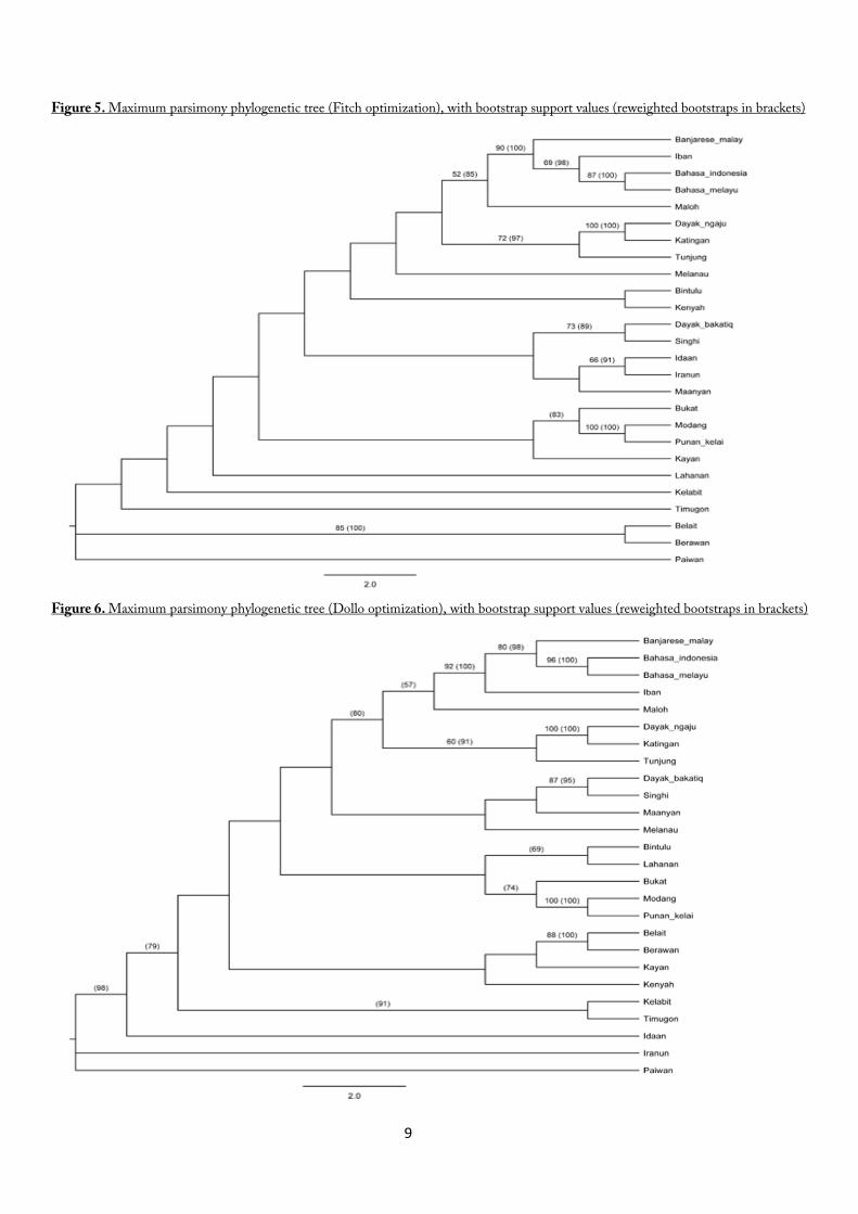
Both Dollo and unordered optimised searches produced one most parsimonious (shortest) tree (MPC) each. The topologies of the two trees can be seen below (Figures 5 and 6). Support values measured from the bootstrap analyses are indicated above the clade branches. Topologies for the reweighted analyses were found to be identical to those of the original, and have their bootstrap values superimposed on the same cladograms (in brackets, Figures 5 and 6). The scores and ensemble indices for the trees can be seen below in Table 2.

Table 2. Maximum parsimony tree score and indices

Unordered Dollo Unordered Reweighted

Dollo Reweighted

# of MPCs 1 1 1 1 Score of MPC 173 231 80.75 110.66 CI 0.357 0.269 0.674 0.563 HI 0.643 0.731 0.326 0.437 RI 0.508 0.786 0.779 0.960 RC 0.182 0.211 0.525 0.540

We find that the Dollo optimised runs typically exhibit a higher fraction of synapomorphy (RI), but also homoplasy (CI, HI), in their characters. The RC indices are more comparable between the two; though with a slight edge towards the Dollo optimised run. We prefer and use RC as the measure of overall character fit here as it does not suffer from some of the drawbacks of CI and RI10, and as it combines both measures of synapomorphy and homoplasy.

9 Our a priori weighting of the characters done initially was not operating

on the assumption that all characters (words) should be weighted equally;

rather it was purely a standardizing procedure to correct the bias of

character-state (cognate) richness on weighting. 10

For example, CI is dependent (inversely proportional) on number of

taxa, inflates with uninformative characters and does not scale down to 0.

Additionally, CI only measures homoplasy while RI only synapomorphy.

9

Figure 5. Maximum parsimony phylogenetic tree (Fitch optimization), with bootstrap support values (reweighted bootstraps in brackets)

Figure 6. Maximum parsimony phylogenetic tree (Dollo optimization), with bootstrap support values (reweighted bootstraps in brackets)

10

We find that posterior weighting dramatically improves the indices of fit across both searches, which is as expected from a character fit based weighting approach. While overall fit (RC) is fairly similar between the unordered and Dollo optimised approaches, tree score is not; Dollo consistently exhibited higher tree scores. However, tree scores are not comparable between the unordered and Dollo methods as they operate (in Paup* 4.0) under differently weighted (transition) stepmatrices (see below, Figure 7).11

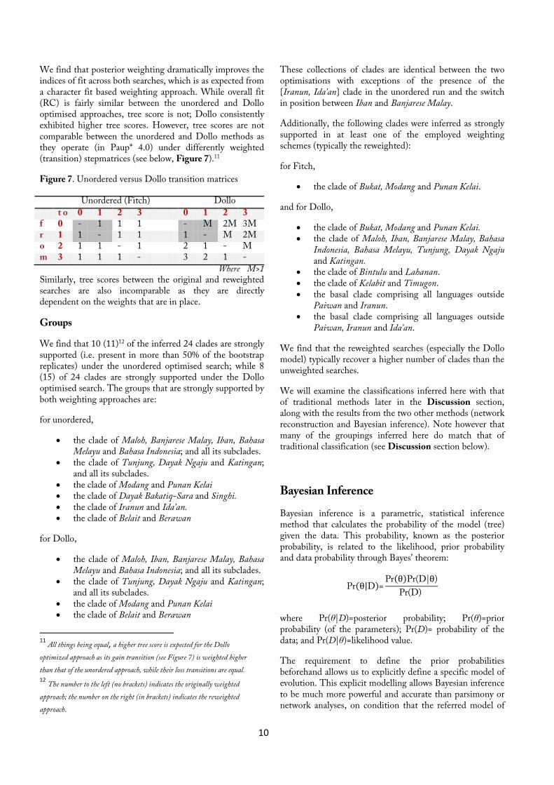
Figure 7. Unordered versus Dollo transition matrices

Unordered (Fitch) Dollo t o 0 1 2 3 0 1 2 3 f 0 - 1 1 1 - M 2M 3M r 1 1 - 1 1 1 - M 2M o 2 1 1 - 1 2 1 - M m 3 1 1 1 - 3 2 1 - Where M>1 Similarly, tree scores between the original and reweighted searches are also incomparable as they are directly dependent on the weights that are in place.

Groups

We find that 10 (11)12 of the inferred 24 clades are strongly supported (i.e. present in more than 50% of the bootstrap replicates) under the unordered optimised search; while 8 (15) of 24 clades are strongly supported under the Dollo optimised search. The groups that are strongly supported by both weighting approaches are:

for unordered,

• the clade of Maloh, Banjarese Malay, Iban, Bahasa Melayu and Bahasa Indonesia; and all its subclades. • the clade of Tunjung, Dayak Ngaju and Katingan; and all its subclades. • the clade of Modang and Punan Kelai • the clade of Dayak Bakatiq-Sara and Singhi. • the clade of Iranun and Ida’an. • the clade of Belait and Berawan

for Dollo,

• the clade of Maloh, Iban, Banjarese Malay, Bahasa Melayu and Bahasa Indonesia; and all its subclades. • the clade of Tunjung, Dayak Ngaju and Katingan; and all its subclades. • the clade of Modang and Punan Kelai • the clade of Belait and Berawan

11

All things being equal, a higher tree score is expected for the Dollo

optimized approach as its gain transition (see Figure 7) is weighted higher

than that of the unordered approach, while their loss transitions are equal. 12

The number to the left (no brackets) indicates the originally weighted

approach; the number on the right (in brackets) indicates the reweighted

approach.

These collections of clades are identical between the two optimisations with exceptions of the presence of the {Iranun, Ida’an} clade in the unordered run and the switch in position between Iban and Banjarese Malay.

Additionally, the following clades were inferred as strongly supported in at least one of the employed weighting schemes (typically the reweighted):

for Fitch,

• the clade of Bukat, Modang and Punan Kelai.

and for Dollo,

• the clade of Bukat, Modang and Punan Kelai. • the clade of Maloh, Iban, Banjarese Malay, Bahasa Indonesia, Bahasa Melayu, Tunjung, Dayak Ngaju and Katingan. • the clade of Bintulu and Lahanan. • the clade of Kelabit and Timugon. • the basal clade comprising all languages outside Paiwan and Iranun. • the basal clade comprising all languages outside Paiwan, Iranun and Ida’an.

We find that the reweighted searches (especially the Dollo model) typically recover a higher number of clades than the unweighted searches.

We will examine the classifications inferred here with that of traditional methods later in the Discussion section, along with the results from the two other methods (network reconstruction and Bayesian inference). Note however that many of the groupings inferred here do match that of traditional classification (see Discussion section below).

Bayesian Inference

Bayesian inference is a parametric, statistical inference method that calculates the probability of the model (tree) given the data. This probability, known as the posterior probability, is related to the likelihood, prior probability and data probability through Bayes’ theorem:

Pr(θ|D)=Pr(θ)Pr(D|θ)

Pr(D)

where Pr(θ|D)=posterior probability; Pr(θ)=prior probability (of the parameters); Pr(D)= probability of the data; and Pr(D|θ)=likelihood value.

The requirement to define the prior probabilities beforehand allows us to explicitly define a specific model of evolution. This explicit modelling allows Bayesian inference to be much more powerful and accurate than parsimony or network analyses, on condition that the referred model of

11

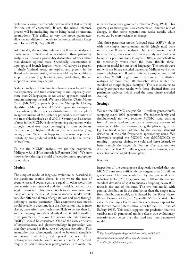
evolution is known with confidence to reflect that of reality (for the set of characters). If not, the whole inference process will be misleading due to being based on unsound assumptions. This ability to vary the model parameters allows many different models to be compared easily (Page and Holmes 1998; Pagel 2000).

Additionally, the resulting inference in Bayesian analysis is much more explicit and representative than parsimony analysis, as it draws a probability distribution of trees rather than discrete ‘optimal trees’. Specifically, uncertainties in topology and branch lengths, which will always be present in single ‘optimal’ trees, are explicit and present in the Bayesian inference results; whereas would require additional support analysis (e.g. bootstrapping, jackknifing, Bremer support) in parsimony analysis.

A direct analysis of this function however was found to be too impractical and time-consuming to run, especially with more than 20 languages, so we use an approach based on random sampling instead. We use a Markov Chain Monte Carlo (MCMC) approach (via the Metropolis Hasting algorithm - Metropolis et al 1953) to generate a sample of trees, whereby the frequency distribution of the sample is an approximation of the posterior probability distribution of the trees (Huelsenbeck et al 2001). Scouting and selection of trees in the MCMC is done by moving via random walks through model tree space, converging to some stationary distribution (of highest likelihood) after a certain (long enough) time. When this happens, the maximum posterior probability tree produced will be implied to be the correct or ‘true’ tree.

To run the MCMC analysis, we use the programme MrBayes v.3.1.2 (Huelsenbeck & Ronquist 2001). We start however by selecting a model of evolution most appropriate for our data.

Models

The simplest model of language evolution, as described in the parsimony section above, is one where the rate of cognate loss and cognate gain are equal. In other words, the rate matrix is symmetrical and the model is defined by a single parameter. This model is obviously simplistic, and likely not very realistic. A more reasonable model would consider differential rates of cognate loss and gain; through defining a second parameter. This asymmetric rate model would be able to accommodate the observation that cognate classes, once arisen, are much more likely to be lost than for another language to independently derive it. Additionally a third parameter, to allow for among site rate variation (ASRV), should be considered. One of the early criticisms of lexicostatistics, and glottochronology in particular, was that they assumed a fixed rate of cognate evolution. This assumption was subsequently found to be overly simplistic and many times false, and opened the need for a heterogeneous distribution of among site rates. A method, frequently used in molecular phylogenetics, is to model the

rates of change via a gamma distribution (Yang 1994). This gamma parameter gives each character an inherent rate of change, so that some cognates can evolve rapidly while others can be more resistant to change.

This three-parameter model (unequal rates+ASRV), along with the simple one-parameter model (single rate) were tested in our Bayesian analyses. The two-parameter model (unequal rates) was excluded from our study as it had been found in a previous study (Luqman 2010, unpublished) to fit consistently worse than the more flexible three-parameter model for our set of languages. The models were run with our binary encoded dataset, as MrBayes (and other current phylogenetic Bayesian inference programmes13) did not allow MCMC algorithms to be run with multistate matrices of more than 10 character states (under the standard or morphological datatype). This also allows us to directly compare our results with those obtained from the parsimony analyses (which used the same binary encoded dataset).

Settings

We ran the MCMC analysis for 10 million generations14, sampling every 1000 generations. We independently and simultaneously ran two separate MCMC runs, starting from different random trees, as a secondary measure of convergence (the first measure being the plateauing of the log likelihood values indicated by the average standard deviation of the split frequencies approaching zero). We Metropolis-coupled the MCMC runs (MCMCMC) by running 4 separate chains; one cold and three heated, to better sample the target distribution. Post analyses, we discarded the first 2.5 million generation as burn-in, after inspection of the log likelihood plots.

Results

Inspection of the convergence diagnostic revealed that our MCMC runs were sufficiently convergent after 10 million generations. This was confirmed by the potential scale reduction factor (PSRF) approaching 1.000 and the average standard deviation of split frequencies dropping below 0.01 towards the end of the runs. The two-rate model with gamma distribution fit the data better than the single-rate, fixed distribution model, as indicated by the Bayes Factor (Bayes Factor = 41.8) (See Appendix A5 for details). This value for the Bayes Factor indicates very strong support for the former model (interpretation after Jeffreys 1961; Kass & Raftery 1995). This result supports our prediction that the variable rate (3-parameter) model reflects true evolutionary scenario much better than the fixed rate (one parameter) model.

13

E.g. BayesPhylogenies (Pagel and Meade, 2004) and BEAST

(Drummond and Rambaut, 2007) were also considered. 14

to allow for sufficient convergence.

12

Figure 8. Bayesian inference 50% majority rule consensus tree (equal rates + no ASRV model), with posterior probabilities

Figure 9. Bayesian inference 50% majority rule consensus tree (unequal rates + ASRV model), with posterior probabilities

13

Above (Figures 8 and 9), we show the two Bayesian inferred trees drawn with their posterior probability values. We see a fair difference at the base and mid-section of the tree topologies, but also a fair number of similarities between the terminal groups of the two models.

Groups

Clades that are common to both models (trees) are the:

• Maloh, Iban, Banjarese Malay, Bahasa Indonesia and Bahasa Melayu clade and subclades ; • Tunjung, Dayak Ngaju and Katingan clade and

subclades; • Belait and Berawan clade; • Bukat and Lahanan clade; • Dayak Bakatiq-Sara and Singhi clade; • Kayan, Modang and Punan Kelai clade.

These clades represent most of the non-basal terminal clades. The topologies at the basal section, represented by Paiwan, Ida’an, Iranun, Kelabit and Timugon, are somewhat conflicting, as are the positions of Ma’anyan and Melanau. We will compare the results obtained here, along with the results from the other tested methods, with the traditional classification in detail in the Discussion section below.

Discussion

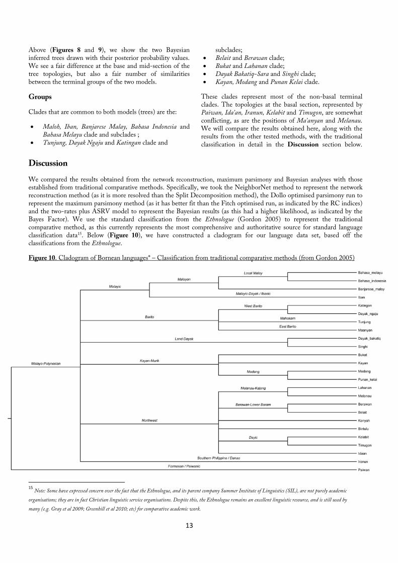
We compared the results obtained from the network reconstruction, maximum parsimony and Bayesian analyses with those established from traditional comparative methods. Specifically, we took the NeighborNet method to represent the network reconstruction method (as it is more resolved than the Split Decomposition method), the Dollo optimised parsimony run to represent the maximum parsimony method (as it has better fit than the Fitch optimised run, as indicated by the RC indices) and the two-rates plus ASRV model to represent the Bayesian results (as this had a higher likelihood, as indicated by the Bayes Factor). We use the standard classification from the Ethnologue (Gordon 2005) to represent the traditional comparative method, as this currently represents the most comprehensive and authoritative source for standard language classification data15. Below (Figure 10), we have constructed a cladogram for our language data set, based off the classifications from the Ethnologue.

Figure 10. Cladogram of Bornean languages* – Classification from traditional comparative methods (from Gordon 2005)

15

Note: Some have expressed concern over the fact that the Ethnologue, and its parent company Summer Institute of Linguistics (SIL), are not purely academic

organisations; they are in fact Christian linguistic service organisations. Despite this, the Ethnologue remains an excellent linguistic resource, and is still used by

many (e.g. Gray et al 2009; Greenhill et al 2010; etc) for comparative academic work.

14

*Note: Maloh is not represented in the above cladogram, as it was absent(due to lack of data) from the Ethnologue.

Of the 13 clades defined in the cladogram above, we find that the Dollo parsimony method correctly recovers 8, while the three-parameter Bayesian model 7. It is difficult to directly compare the NN network diagram to the tree diagram above, for obvious topographical reasons. However, at least 5 traditional clades ({Punan Kelai and Modang}, {Dayak Ngaju and Katingan}, {Belait and Berawan} and the {Iban, Banjarese Malay, {Bahasa Melayu and Bahasa Indonesia}} complex) are evidently present in the NN network diagram. Additionally, we find that all three methods tested correctly recover:

1. the Malayic group and sub-groups; composed of Iban, Banjarese Malay, Bahasa Melayu and Bahasa Indonesia.

2. the Barito sub-group of West Barito and Mahakam; represented by Tunjung, Dayak Ngaju and Katingan.

3. the Land Dayak group; composed of Dayak Bakatiq-Sara and Singhi.

4. the Modang subgroup; of Modang and Punan Kelai. 5. the Berawan-Lower Baram subgroup; of Belait and

Berawan.

Both maximum parsimony bootstrap values and Bayesian posterior probability values strongly support the above five groups and subgroups.

The groups that are most ambiguous are the Northwest and Kayan-Murik groups, as well as the position of the Ma’anyan language. We have constant rearrangement in their positions and compositions across the tree topologies, though the languages Kelabit, Timugon, Ida’an and Iranun are consistently recovered as basal. It is difficult to assess and compare the more basal clades across topologies as the standard classification has many of them as unresolved (under the Malayo-Polynesian node). If we remove all unresolved clades (i.e. clades that multi-furcate into more than two braches), we find that the maximum parsimony method correctly recovers 8 out of 9 possible clades, while Bayesian inference method, 7 out of 9.

This is a remarkably good match for both tested methods. It may be tempting to conclude that the maximum parsimony approach is the more accurate of the two methods, as it matched the traditional classification better, but this would be a hasty and unsound judgement. It is difficult to compare and justifyingly select tree topologies between the parsimony and Bayesian approaches, as their trees are described under different indices of fit (RC values for the former, likelihood values for the latter). One possible way to approach this is to measure the topological distance between the traditional tree and the test tree (via e.g. the Robinson-Foulds distance (Robinson & Foulds 1981)) and select the tree with least topological distance. However, this is potentially misrepresentative with non-fully resolved trees (such as our traditional classification tree), and operates under the heavy assumption that the

traditional tree is in fact the true tree, so cannot be considered further here.

There are of course some non-trivial differences between the topologies of the tested methods and the traditional method (specifically, the remaining unrecovered clades). Whether these differences reflect a disparity in method, models, characters, wordlists or prior assumptions is unclear. Any or all of these aspects could have distanced our tree from the true one. For example, our character number and selection was far from ideal. We did not include phonological or grammatical characters, and reduced our lexical characters to only 64 units. With a revised and updated wordlist, along with inclusion of phonological and grammatical characters, it may be possible to gain up to 300 representative characters for our set of languages. More and varying types of characters have been shown (Hillis 1998; Page & Holmes 1998; Scotland et al 2003; Wortley & Scotland 2006) to improve both phylogenetic accuracy and support.

Additionally, some (e.g. Poser 2003) have expressed scepticism on any purely lexical-based approach, with reason that lexical change is much more subject to cultural influence than other aspects of language change. Nakhleh et al 2005 for example, have shown that including these other aspects of linguistic change typically result in different and improved phylogenetic inferences.

Nevertheless, it is remarkable and supportive to find that the two phylogenetic methods tested (maximum parsimony and Bayesian inference), which operate under such different methodologies, can match traditional classification so well. The close approximation between the classifications inferred from these two methods with that established from the traditional comparative method is suggestive that such phylogenetic approaches can be used to infer language evolutionary history16. Such quantitative and computational methods are advantageous over traditional ones in that they can be run much more quickly and objectively, and are explicit in their confidence. The model plasticity of the Bayesian method in particular, holds a wealth of untapped potential. Different linguistic evolutionary scenarios can be tested and compared, and the site rate heterogeneity allows us to model time-calibrated evolution. This among site rate heterogeneity is key as it has been shown (e.g. Pagel et al 2007; Greenhill et al 2010) that word evolution rate is not fixed, rather it is variable. Gray & Atkinson (2003) and Gray et al (2009) have led the way in this approach by using a gamma distribution to model site rate variation and consequently infer evolutionary time; though how accurate this method is is still uncertain. Nonetheless, the potential is there, and such inference power opens the door to many possibilities. Questions regarding the time of divergence events, age of languages, rates of cultural and linguistic change, age and homeland (geographical origin) of

16 On condition of little or insignificant horizontal transmission.

15

language families, and even human expansion, migration and settlement scenarios can all be addressed by such time calibrated models. These are questions not only interesting to linguists and biologists, but to all of humanity.

Acknowledgements

I would like to thank my supervisor, Dr. Margaret Clegg, for providing guidance and helpful comments throughout the course of this project.

References

• Atkinson, Q.D. & Gray, R.D. (2006) How old is the Indo-

European language family? Progress or more moths to the

flame? In: Phylogenetic Methods and the Prehistory of Languages.

Cambridge: The McDonald Institute for Archaeological

Research, 91-109.

• Atkinson, Q.D., Meade, A., Venditti, C., Greenhill, S.J., &

Pagel, M. (2008) Languages evolve in punctuational bursts.

Science 319, 588.

• Bateman, R., Goddard, I., O’Grady, R., Funk, V. A., Mooi, R.,

Kress, W. J. & Cannell, P. (1990) Speaking of forked tongues:

the feasibility of reconciling human phylogeny and the history of

language. Current Anthropology 31, 1–24.

• Bellwood, P. (1996) Phylogeny vs. reticulation in prehistory.

Antiquity 70, 881–890.

• Bellwood, Peter (1997) Prehistory of the Indo-Malaysian

archipelago. Honolulu: University of Hawai'i Press.

• Blust, R. (1999)"Subgrouping, circularity and extinction: some

issues in Austronesian comparative linguistics" in E. Zeitoun &

P.J.K Li (Ed.) Selected papers from the Eighth International

Conference on Austronesian Linguistics (pp. 31-94). Taipei:

Academia Sinica.

• Borgerhoff Mulder, M. (2001) Using phylogenetically base

comparative methods in anthropology: more questions than

answers. Evolutionary Anthropology 10, 99–111.

• Bryant, D. & Moulton, V. (2004) NeighborNet: An

agglomerative method for the construction of phylogenetic

networks. Molecular Biology and Evolution, 21:255-265.

• Darwin, Charles (1871). The descent of man. Murray, London.

• Dawkins R. (1982) The Extended Phenotype. Oxford, UK:

Freeman

• Dawkins R. (1989) The Selfish Gene. New York: Oxford

University Press. 2nd edition.

• Drummond A.J. & Rambaut, A. (2007) BEAST: Bayesian

evolutionary analysis by sampling trees. BMC Evolutionary

Biology 7:214.

• Evans, S.N., D. Ringe, and T. Warnow, (2006) ‘Inference of

divergence times as a statistical inverse problem.’ Book chapter

in “Phylogenetic Methods and the Prehistory of Languages," pp.

119-129. Edited by Peter Forster and Colin Renfrew. Edited for

the Institute by Chris Scarre (Series Editor) and Dora A. Kemp

(Production Editor). Publisher: McDonald Institute for

Archaeological Research/University of Cambridge, 2006.

• Farris, J. S. (1977) Phylogenetic analysis under Dollo’s Law.

Systematic Zoology 26, 77–88.

• Farris,]. S. (1983) The logical basis of phylogenetic analysis. In:

N. Platnick and V. Funk (eds), Advances in Cladistics.

Proceedings of the second meeting of the Willi Hennig Society.

Vol. 2: Columbia Univ. Press, New York: 7-36.

• Gordon, R.G. (2005) Ethnologue: Languages of the World, 15th

edition. Dallas, Tex.: SIL International.

• Gould, S. J. (1987) An urchin in the storm. New York, NY:

Norton.

• Gould, S. J. (1991) Bully for brontosaurus. New York, NY:

Norton.

• Gray, R.D. & F.M. Jordan. (2000) Language trees support the

express-train sequence of Austronesian expansion. Nature 405,

1052-1055.

• Gray, R.D., Drummond, A.J., & Greenhill, S.J. (2009)

Language Phylogenies Reveal Expansion Pulses and Pauses in

Pacific Settlement. Science 323: 479-483.

• Gray, RD, Greenhill, SJ, & Ross, RM (2007) The Pleasures

and Perils of Darwinizing Culture (with phylogenies). Biological

Theory, 2(4).

• Gray, Russell D. & Quentin D. Atkinson (2003) Language-tree

divergence times support the Anatolian theory of Indo-

European origin. Nature 426: 435-439.

• Greenhill SJ, Atkinson QD, Meade A, & Gray RD. (2010) The

shape and tempo of language evolution. Proceedings of the Royal

Society, B.

• Greenhill, S.J., Blust. R, & Gray, R.D. (2008). The

Austronesian Basic Vocabulary Database: From Bioinformatics

to Lexomics. Evolutionary Bioinformatics, 4:271-283.

• Gudschinsky, Sarah C. (1956) The ABC’s of lexicostatistics

(glottochronology). Word 12: 175-210.

• Hillis, D. M. (1998) Taxonomic sampling, phylogenetic

accuracy, and investigator bias. Systematic Biology 47:3-8.

16

• Hoenigswald, H. M. (1960) Language Change and Linguistic

Reconstruction. University of Chicago Press, Chicago.

• Hoijer H (1956) Lexicostatistics: a critique. Language 32:49–60.

• Holden, C. J. & Shennan, S. (2005) How tree-like is cultural

evolution? In The evolution of cultural diversity: phylogenetic

approaches (eds R. Mace, C. J. Holden & S. Shennan), pp. 13–

29. London, UK: UCL Press.

• Holden, C.J. & Gray, R.D. (2006) Exploring Bantu linguistic

relationships using trees and networks. In: Phylogenetic Methods

and the Prehistory of Languages. Forster, P & Renfrew, C. (eds).

Cambridge: The McDonald Institute for Archaeological

Research, pp. 19-31.

• Holden, Clare Janaki (2002) Bantu language trees reflect the

spread of farming across sub-Saharan Africa: a maximum-

parsimony analysis. Proceedings of the Royal Society B: Biological

Sciences 269(1493): 793-799.

• Huelsenbeck, J. P., and F. Ronquist (2001) MrBayes: Bayesian

inference of phylogeny. Bioinformatics 17:754–755.

• Huelsenbeck, J. P., F. Ronquist, R. Nielsen, and J. P. Bollback

(2001) Bayesian inference of phylogeny and its impact on

evolutionary biology. Science 294:2310.

• Hull D. L. (1988) Science as a Process: An Evolutionary Account of

the Social and Conceptual Development of Science. Chicago, IL:

University of Chicago Press.

• Hull D. L. (2001) Science and Selection: Essays on Biological

Evolution and the Philosophy of Science. Cambridge, UK:

Cambridge University Press.

• Huson, Daniel H. & Byrant, David (2006) Application of

Phylogenetic Networks in Evolutionary Studies. Molecular

Biology and Evolution 23(2):254-267.

• Jeffreys, H. (1961) The Theory of Probability (3e), Oxford; p. 432

• Kass, R.E. & Raftery, A.E. (1995) Bayes Factors. Journal of the

American Statistical Association 430:773-795.

• Kitchen, Andrew, Christopher Ehret, Shiferaw Assefa &

Connie J. Mulligan (2009) Bayesian phylogenetic analysis of

Semitic languages identifies an Early Bronze Age origin of

Semitic in the Near East. Proceedings of the Royal Society B

276:2703-2710.

• Lewis, M. Paul (2009) Ethnologue: Languages of the World,

Sixteenth edition. Dallas, Tex.: SIL International.

• Metropolis, N.; Rosenbluth, A.W.; Rosenbluth, M.N.; Teller,

A.H.; Teller, E. (1953) Equations of State Calculations by Fast

Computing Machines. Journal of Chemical Physics 21 (6): 1087–

1092.

• Moore, J. H. (1994) Putting anthropology back together again:

the ethnogenetic critique of cladistic theory. American

Anthropologist 96, 925–948.

• Nakhleh, Luay, Tandy Warnow, Don Ringe & Steven N. Evans

(2005a) A comparison of phylogenetic reconstruction methods

on an Indo-European dataset. Transactions of the Philological

Society 103(2): 171-192.

• Nicholls, G.K. & Gray, R.D. (2006) Quantifying uncertainty in

a stochastic Dollo model of vocabulary evolution. In:

Phylogenetic Methods and the Prehistory of Languages. Cambridge:

The McDonald Institute for Archaeological Research, 161-172.

• Page, R. D. M., and E. C. Holmes (1998) Molecular evolution:

Phylogenetic approach. University Press, Cambridge.

• Pagel, M. & Meade, A. (2004) A phylogenetic mixture model

for detecting pattern heterogeneity in gene sequence or

character-state data. Systematic Biology 53: 571-581.

• Pagel, Mark (2000) Maximum-likelihood models for

glottochronology and for reconstructing linguistic phylogenies.

In: Colin Renfrew, April McMahon, & Larry Trask (eds.) Time

depth in historical linguistics. Cambridge: McDonald Institute for

Archaeological Research, 189-207.

• Pagel, Mark, Quentin D. Atkinson & Andrew Meade (2007)

Frequency of word-use predicts rates of lexical evolution

throughout Indo-European history. Nature 449(7163): 717-720.

• Poser, B. (2003) Dating Indo-European. Language Log.

• Rexová, Kateřina, Daniel Frynta & Jan Zrzavy (2002) Cladistic

analysis of languages: Indo-European classification based on

lexicostatistical data. Cladistics 19: 120-127.

• Rexová, Kateřina, Yvonne Bastin & Daniel Frynta (2006)

Cladistic analysis of Bantu languages: a new tree based on

combined lexical and grammatical data. Naturwissenschaften

93(4): 189-194.

• Robinson, D.R & Foulds, L.R. (1981) Comparison of

phylogenetic trees. Mathematical Biosciences 53, p. 131-147.

• Scotland, R. W, R. G. Olmstead, and J. R. Bennett. (2003b)

Phylogeny reconstruction: The role of morphology. Systematic

Biology 52:539-548.

• Scotland, Robert W. and Wortley, Alexandra H. (2006) The

Effect Combing Molecular and Morphological Data in

Published Phylogenetic Analyses. Systematic Biology 55(4):677-

685.

• Swadesh, Morris (1952) Lexico-Statistic Dating of Prehistoric

Ethnic Contacts: With Special Reference to North American

Indians and Eskimos. Proceedings of the American Philosophical

Society 96(4): 452-463.

17

• Swofford, D.L. (2000) PAUP, Version 4.0b4a. Sinauer,

Sunderland, MA.

• Swofford, David L. And Begle, Douglas P (2003) Phylogenetic

Analysis Using Parsimony (PAUP) Version 3.1 User’s Manual.

Laboratory of Molecular Systematics. Smithsonian Institution.

• Temkin, I. & Eldredge, N. (2007) Phylogenetics and material

cultural evolution. Current Anthropology 48, 146–153.

• Terrell, J. E. (1988) History as a family tree, history as an

entangled bank: constructing images and interpretations of

prehistory in the South Pacific. Antiquity 62, 642–657.

• Terrell, J. E., Kelly, K. M. & Rainbird, R. (2001) Foregone

conclusions? In search of ‘Papuans’ and ‘Austronesians’. Current

Anthropology 42, 97–124.

• Trejaut J. A., Kivisild T., Loo J.H., Lee C.L., He C.L., Hsu,

C.J., Li, Z.Y. and Lin, M. (2005) Traces of archaic

mitochondrial lineages persist in Austronesian-speaking

Formosan populations. PLoS Biology 3(8): e247.

• Warnow, T., Evans, S. N., Ringe, D., & Nakhleh, L., (2004) A

Stochastic model of language evolution that incorporates

homoplasy and borrowing. In Peter Forster, Colin Renfrew and

James Clackson (eds.) Phylogenetic Methods and the Prehistory of

Languages. Cambridge: McDonald Institute for Archaeological

Research.

• Wortley, A.H. & R.W. Scotland. 2006. The effect of

combining molecular and morphological data in published

phylogenetic analyses. Systematic Biology 55(4): 677-685.

• Yang, Z. (1994) Maximum likelihood phylogenetic estimation

from DNA sequences with variable rates over sites:

Approximate methods. Journal of Molecular Evolution 39:306–

314.

Appendix

A1. Language List

1. Banjarese Malay

2. Belait

3. Berawan (Long Terawan)

4. Bintulu

5. Bukat

6. Dayak Bakatiq-Sara/Riok

7. Dayak Ngaju

8. Iban

9. Ida’an

10. Iranun

11. Katingan

12. Kayan (Uma Juman)

13. Kelabit (Bario)

14. Kenyah (Long Anap)

15. Lahanan

16. Ma’anyan

17. Bahasa Indonesia

18. Maloh

19. Melanau (Mukah)

20. Bahasa Melayu

21. Modang

22. Punan Kelai

23. Singhi

24. Timugon (Murut)

25. Tunjung

26. Paiwan (Outgroup)

A2. Austronesian Basic Vocabulary Database Wordlist (filtered)

Words used in study are indicated in bold. For word selection criteria, refer to Section 4 under Methods & Materials.

1. hand 36. to spit 71. to stab, pierce 106. snake 141. wet 176. below

2. left 37. to eat 72. to hit 107. worm 142. heavy 177. this

3. right 38. to chew 73. to steal 108. louse 143. fire 178. that

4. leg/foot 39. to cook 74. to kill 109. mosquito 144. to burn 179. near

5. to walk 40. to drink 75. to die, be dead 110. spider 145. smoke 180. far

6. road/path 41. to bite 76. to live, be alive 111. fish 146. ash 181. where?

7. to come 42. to suck 77. to scratch 112. rotten 147. black 182. I

8. to turn 43. Ear 78. to cut, hack 113. branch 148. white 183. thou

9. to swim 44. to hear 79. stick/wood 114. leaf 149. red 184. he/she

10. Dirty 45. Eye 80. to split 115. root 150. yellow 185. we

11. dust 46. to see 81. sharp 116. flower 151. green 186. you

12. skin 47. to yawn 82. dull, blunt 117. fruit 152. small 187. they

13. back 48. to sleep 83. to work 118. grass 153. big 188. what?

14. belly 49. to lie down 84. to plant 119. earth/soil 154. short 189. who?

15. bone 50. to dream 85. to choose 120. stone 155. long 190. other

16. intestines 51. to sit 86. to grow 121. sand 156. thin 191. all

17. liver 52. to stand 87. to swell 122. water 157. thick 192. and

18. breast 53. person/human being 88. to squeeze 123. to flow 158. narrow 193. if

19. shoulder 54. man/male 89. to hold 124. sea 159. wide 194. how?

20. to know 55. woman/female 90. to dig 125. salt 160. painful, sick 195. no, not

21. to think 56. child 91. to buy 126. lake 161. shy, ashamed 196. to count

22. to fear 57. husband 92. to open, uncover 127. woods/forest 162. old 197. One

23. blood 58. wife 93. to pound, beat 128. sky 163. new 198. Two

24. head 59. mother 94. to throw 129. moon 164. good 199. Three

25. neck 60. father 95. to fall 130. star 165. bad, evil 200. Four

26. hair 61. house 96. dog 131. cloud 166. correct, true 201. Five

27. nose 62. thatch/roof 97. bird 132. fog 167. night 202. Six

28. to breathe 63. name 98. egg 133. rain 168. day 203. Seven

29. to sniff, smell 64. to say 99. feather 134. thunder 169. year 204. Eight

30. mouth 65. rope 100. wing 135. lightning 170. when? 205. Nine

31. tooth 66. to tie up, fasten 101. to fly 136. wind 171. to hide 206. Ten

32. tongue 67. to sew 102. rat 137. to blow 172. to climb 207. Twenty

33. to laugh 68. needle 103. meat/flesh 138. warm 173. at 208. Fifty

34. to cry 69. to hunt 104. fat/grease 139. cold 174. in, inside 209. One Hundred

35. to vomit 70. to shoot 105. tail 140. dry 175. above 210. One Thousand

A3.  Multistate Matrix 

   1  2  3 4 5 6  7  8  9  10 11 12 13 14 15 16 17 18 19 20 21  22  23 24 25 26 27 28 29 30 31 32 Character  Key   Banjarese Malay  2  5  1  1  1  1  2  1  1  6  3  1  5  3  2  1  1  2  1  1  1  1  1  2  1  1  4  2  1  1  1  4    1 Hand  55  Night Belait  2  4  2  1  1  1  1  1  2  3  1  1  3  1  1  4  1  1  1  3  1  3  1  3  1  1  1  1  3  3  1  1    2 Left  56  When Berawan  6  2  2  1  1  1  1  3  2  3  1  1  3  1  1  1  1  1  1  4  3  4  1  1  1  1  1  1  3  4  3  1    3 Right  57  Where Bintulu  4  2  2  3  1  1  5  4  1  3  1  1  6  1  1  1  1  1  3  5  1  5  1  4  1  1  1  1  1  5  4  1    4 Road  58  What Bukat  7  2  2  4  2  1  4  1  1  7  ?  1  1  5  1  5  1  1  1  6  4  1  1  1  ?  1  1  1  2  6  5  1    5 Skin  59  Who Dayak Bakatiq  8  1  2  2  1  1  1  5  1  8  1  3  1  6  3  6  2  3  1  7  5  1  1  5  2  1  5  1  3  7  6  1    6 Bone  60  One Dayak Ngaju  3  3  2  2  3  1  2  2  1  4  2  1  2  2  1  1  1  1  1  2  2  2  1  1  1  1  6  3  1  3  1  1    7 Shoulder  61  Two Iban  2  6  1  1  1  1  2  1  1  9  1  1  ?  7  1  1  3  1  1  2  2  1  1  1  1  1  2  2  1  1  1  1    8 Fear  62  Three Ida'an  9  4  1  1  1  1  6  6  1  1  1  1  7  1  1  7  4  1  1  1  1  1  1  1  1  1  1  1  4  1  1  1    9 Blood  63  Four Iranun  1  4  1  1  5  1  1  7  3  1  1  2  8  1  1  8  5  1  1  1  1  6  1  1  3  2  1  1  4  1  1  1    10 Neck  64  Five Katingan  3  3  2  2  3  1  2  2  1  4  2  1  2  2  1  1  1  1  1  2  2  2  1  1  1  1  2  3  1  3  1  1    11 Hair     Kayan  10  2  2  1  2  1  3  1  1  10  1  1  1  1  1  9  1  1  1  8  6  7  1  1  1  1  1  1  1  2  1  1    12 Nose     Kelabit  6  4  4  1  2  1  7  1  1  1  1  1  9  1  1  10  1  1  1  2  7  1  1  6  1  1  1  1  1  8  1  2    13 Mouth     Kenyah  11  4  2  1  2  1  3  1  1  3  1  1  1  1  1  1  1  1  1  3  1  8  1  7  1  1  7  1  1  2  1  1    14 Tooth     Lahanan  12  2  2  3  6  1  4  1  1  2  1  1  1  1  1  2  1  1  1  9  8  1  1  8  ?  1  1  1  2  3  7  1    15 Tongue     Ma'anyan  2  1  1  1  1  1  1  8  1  11  4  1  1  1  1  11  6  1  1  10  9  1  1  9  1  3  1  1  2  1  1  1    16 Laugh     B. Indonesia  2  1  1  1  1  1  2  1  1  1  3  1  4  3  1  1  1  1  1  1  1  1  1  1  1  1  3  2  1  1  1  3    17 Cry     Maloh  2  7  2  1  1  1  4  1  1  5  1  4  1  8  1  1  1  1  1  1  1  1  1  1  4  1  2  1  5  1  1  1    18 Vomit     Melanau  4  2  2  1  1  1  1  9  1  2  1  1  1  1  1  1  1  1  1  11  1  1  1  1  1  1  1  1  2  1  1  1    19 Eat     B. Melayu  2  1  1  1  1  1  2  1  1  1  3  1  4  3  1  1  1  1  1  1  1  1  1  1  1  1  3  2  1  1  1  3    20 Drink     Modang  5  2  3  1  4  1  3  1  1  12  1  1  1  4  1  3  1  1  2  12  1  2  1  1  1  1  1  1  3  2  2  5    21 Ear     Punan Kelai  5  8  3  1  4  1  3  1  1  13  1  1  5  4  1  3  1  1  2  13  10  2  1  1  1  1  1  1  3  9  2  1    22 Hear     Singhi  2  9  2  1  1  1  8  10  1  2  1  1  1  1  1  1  7  1  1  1  11  1  2  10  5  1  1  1  ?  10  8  6    23 Eye     Timugon  3  10  5  1  7  1  1  11  1  1  1  1  10  1  1  12  1  4  1  1  1  1  1  11  1  1  1  1  4  3  1  2    24 Sleep     Tunjung  2  2  2  1  1  2  ?  12  1  5  2  1  11  2  1  1  1  1  1  14  12  9  3  1  ?  4  8  1  ?  3  1  7    25 Dream     Paiwan  1  1  1  1  2  1  1  1  4  1  5  2  12  9  4  2  1  1  1  15  1  10  1  12  1  1  1  1  1  2  1  1    26 Child      Continued..  33  34  35 36 37 38  39  40  41  42 43 44 45 46 47 48 49 50 51 52 53  54  55 56 57 58 59 60 61 62 63 64 28 Father     Banjarese Malay  2  1  2  2  2  6  1  2  2  1  1  5  ?  1  1  1  1  1  1  1  1  1  2  3  3  1  2  1  1  1  1  1    29 House     Belait  1  1  1  3  1  4  1  3  4  2  1  6  5  1  1  2  ?  2  2  2  1  2  2  4  5  5  1  1  1  1  1  1    30 Kill     Berawan  1  1  1  1  1  4  1  3  4  3  1  7  6  2  1  3  1  1  3  3  1  1  2  1  6  2  1  1  1  1  1  1    31 Die     Bintulu  1  1  3  1  1  7  1  ?  1  4  1  ?  4  1  1  1  3  1  1  1  1  3  2  5  5  2  1  3  1  1  1  ?    32 Dog     Bukat  4  1  4  1  3  8  1  2  3  1  1  2  1  3  ?  4  1  3  ?  4  1  1  2  2  7  2  1  4  1  1  1  ?    33 Bird     Dayak Bakatiq  1  2  5  1  4  1  1  ?  1  1  1  1  7  1  1  1  4  1  1  1  1  1  4  1  8  6  4  1  1  1  1  1    34 Egg     Dayak Ngaju  2  1  1  1  1  2  1  1  2  1  1  ?  1  1  1  1  2  1  1  1  1  1  2  6  4  3  3  1  1  1  1  1    35 Rat     Iban  2  1  2  1  2  1  1  1  1  1  1  1  2  1  1  1  1  1  1  1  1  1  2  7  9  ?  2  2  1  2  1  1    36 Tail     Ida'an  5  3  6  1  2  5  1  2  5  1  1  2  8  1  1  1  5  1  4  1  1  1  3  1  5  2  5  1  1  1  1  1    37 Snake     Iranun  6  4  7  1  5  9  1  4  6  5  1  8  9  1  1  1  1  1  1  1  2  1  3  8  10  7  6  1  1  1  1  1    38 Fish     Katingan  2  5  1  1  1  2  1  1  2  1  1  2  1  1  1  1  2  1  1  1  1  1  2  9  4  3  3  1  1  1  1  1    39 Leaf     Kayan  1  1  1  1  1  10  1  2  ?  1  1  9  10  1  1  5  6  1  1  1  1  1  2  1  1  2  1  1  1  1  1  1    40 Root     Kelabit  1  1  1  1  6  11  1  ?  4  1  1  10  4  1  1  1  7  1  1  1  1  1  1  1  11  2  1  5  1  1  1  1    41 Flower     Kenyah  3  1  1  1  2  3  ?  2  ?  1  1  11  11  1  1  1  1  1  1  1  1  4  2  1  5  2  1  1  1  1  1  1    42 Fruit     Lahanan  1  1  1  1  1  1  1  3  3  1  1  12  1  1  ?  1  8  1  ?  1  1  1  2  10  12  2  ?  1  1  1  1  ?    43 Stone     Ma'anyan  2  1  8  1  1  12  1  2  1  1  1  4  1  1  1  6  1  1  ?  5  1  1  2  11  13  2  1  1  1  1  1  1    44 Sand     B. Indonesia  2  1  2  1  2  1  1  ?  1  1  1  1  2  1  1  1  1  1  1  1  1  1  2  3  3  1  2  2  1  2  1  1    45 Water     Maloh  2  1  1  1  2  2  1  1  1  1  1  4  1  4  1  1  9  1  1  ?  1  1  2  12  14  1  7  1  1  1  1  ?    46 Sky     Melanau  1  1  1  1  1  1  1  ?  1  1  1  13  1  1  1  1  ?  1  1  1  1  1  2  13  15  2  1  ?  1  1  1  1    47 Moon     B. Melayu  2  1  2  1  2  1  1  2  1  1  1  1  2  1  1  1  1  1  1  1  1  1  2  3  3  1  2  2  1  2  1  1    48 Star     Modang  1  1  9  1  1  3  2  2  7  1  1  3  3  1  1  7  1  1  5  1  1  1  2  2  2  2  1  1  2  1  1  ?    49 Cloud     Punan Kelai  1  1  10  1  1  3  2  1  1  1  1  3  3  1  1  8  1  1  1  1  1  1  2  2  2  2  8  1  3  1  1  ?    50 Rain     Singhi  1  1  11  1  1  1  1  ?  ?  1  1  1  12  1  1  1  1  1  1  1  1  1  4  14  16  2  1  1  1  1  1  ?    51 Lightning     Timugon  3  1  2  1  7  5  1  2  4  6  1  14  13  5  1  1  1  4  6  1  1  1  1  1  17  8  1  1  1  1  1  ?    52 Wet     Tunjung  7  1  ?  1  1  13  1  2  1  1  1  1  1  1  ?  1  1  1  ?  1  1  1  2  1  18  4  9  1  2  1  1  1    53 Heavy     Paiwan  8  1  1  1  8  14  3  5  8  7  2  15  1  6  2  1  10  1  7  6  3  1  5  1  1  4  10  1  1  1  1  1    54 Fire     

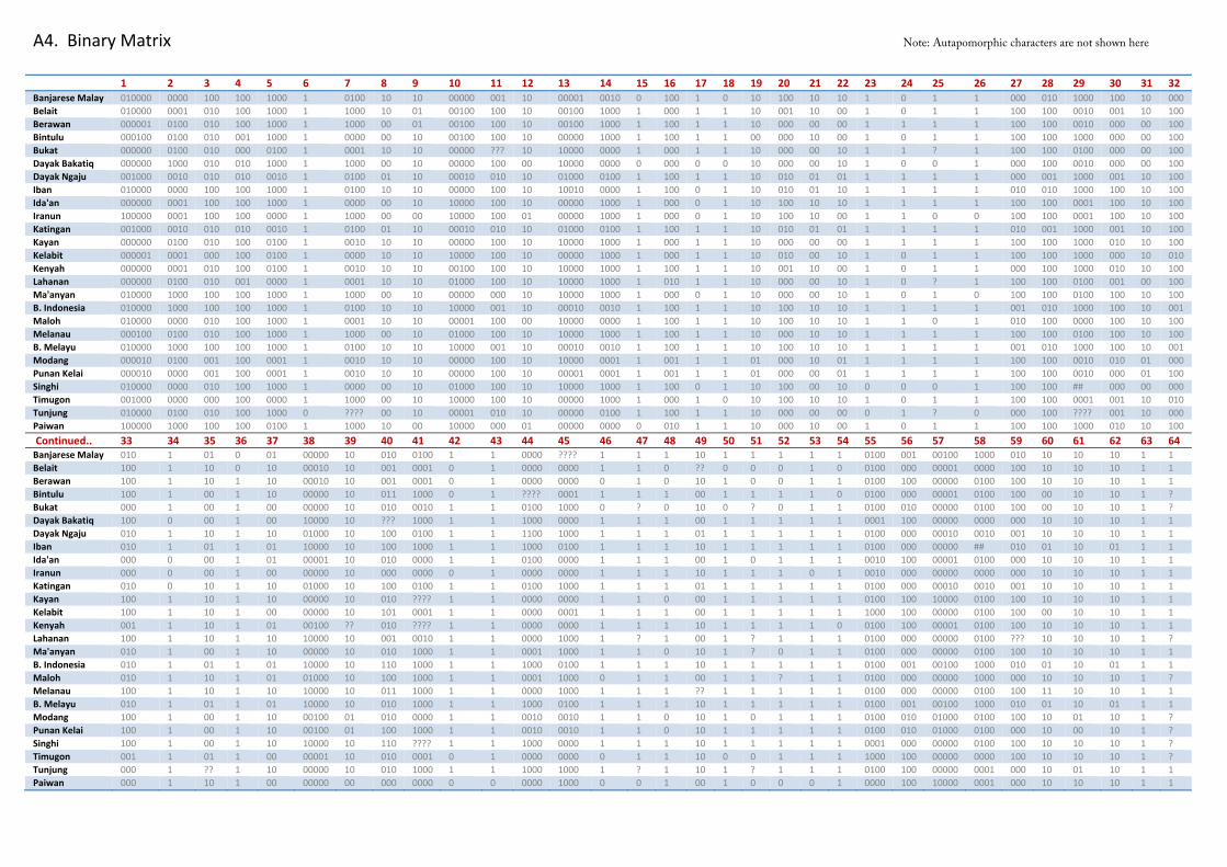
A4.  Binary Matrix                                   Note: Autapomorphic characters are not shown here

   1  2  3 4 5  6  7  8 9 10 11 12 13 14 15 16  17  18 19 20 21 22 23 24 25 26 27 28 29  30  31  32 Banjarese Malay  010000  0000  100  100  1000  1  0100  10  10  00000  001  10  00001  0010  0  100  1  0  10  100  10  10  1  0  1  1  000  010  1000  100  10  000 Belait  010000  0001  010  100  1000  1  1000  10  01  00100  100  10  00100  1000  1  000  1  1  10  001  10  00  1  0  1  1  100  100  0010  001  10  100 Berawan  000001  0100  010  100  1000  1  1000  00  01  00100  100  10  00100  1000  1  100  1  1  10  000  00  00  1  1  1  1  100  100  0010  000  00  100 Bintulu  000100  0100  010  001  1000  1  0000  00  10  00100  100  10  00000  1000  1  100  1  1  00  000  10  00  1  0  1  1  100  100  1000  000  00  100 Bukat  000000  0100  010  000  0100  1  0001  10  10  00000  ???  10  10000  0000  1  000  1  1  10  000  00  10  1  1  ?  1  100  100  0100  000  00  100 Dayak Bakatiq  000000  1000  010  010  1000  1  1000  00  10  00000  100  00  10000  0000  0  000  0  0  10  000  00  10  1  0  0  1  000  100  0010  000  00  100 Dayak Ngaju  001000  0010  010  010  0010  1  0100  01  10  00010  010  10  01000  0100  1  100  1  1  10  010  01  01  1  1  1  1  000  001  1000  001  10  100 Iban  010000  0000  100  100  1000  1  0100  10  10  00000  100  10  10010  0000  1  100  0  1  10  010  01  10  1  1  1  1  010  010  1000  100  10  100 Ida'an  000000  0001  100  100  1000  1  0000  00  10  10000  100  10  00000  1000  1  000  0  1  10  100  10  10  1  1  1  1  100  100  0001  100  10  100 Iranun  100000  0001  100  100  0000  1  1000  00  00  10000  100  01  00000  1000  1  000  0  1  10  100  10  00  1  1  0  0  100  100  0001  100  10  100 Katingan  001000  0010  010  010  0010  1  0100  01  10  00010  010  10  01000  0100  1  100  1  1  10  010  01  01  1  1  1  1  010  001  1000  001  10  100 Kayan  000000  0100  010  100  0100  1  0010  10  10  00000  100  10  10000  1000  1  000  1  1  10  000  00  00  1  1  1  1  100  100  1000  010  10  100 Kelabit  000001  0001  000  100  0100  1  0000  10  10  10000  100  10  00000  1000  1  000  1  1  10  010  00  10  1  0  1  1  100  100  1000  000  10  010 Kenyah  000000  0001  010  100  0100  1  0010  10  10  00100  100  10  10000  1000  1  100  1  1  10  001  10  00  1  0  1  1  000  100  1000  010  10  100 Lahanan  000000  0100  010  001  0000  1  0001  10  10  01000  100  10  10000  1000  1  010  1  1  10  000  00  10  1  0  ?  1  100  100  0100  001  00  100 Ma'anyan  010000  1000  100  100  1000  1  1000  00  10  00000  000  10  10000  1000  1  000  0  1  10  000  00  10  1  0  1  0  100  100  0100  100  10  100 B. Indonesia  010000  1000  100  100  1000  1  0100  10  10  10000  001  10  00010  0010  1  100  1  1  10  100  10  10  1  1  1  1  001  010  1000  100  10  001 Maloh  010000  0000  010  100  1000  1  0001  10  10  00001  100  00  10000  0000  1  100  1  1  10  100  10  10  1  1  0  1  010  100  0000  100  10  100 Melanau  000100  0100  010  100  1000  1  1000  00  10  01000  100  10  10000  1000  1  100  1  1  10  000  10  10  1  1  1  1  100  100  0100  100  10  100 B. Melayu  010000  1000  100  100  1000  1  0100  10  10  10000  001  10  00010  0010  1  100  1  1  10  100  10  10  1  1  1  1  001  010  1000  100  10  001 Modang  000010  0100  001  100  0001  1  0010  10  10  00000  100  10  10000  0001  1  001  1  1  01  000  10  01  1  1  1  1  100  100  0010  010  01  000 Punan Kelai  000010  0000  001  100  0001  1  0010  10  10  00000  100  10  00001  0001  1  001  1  1  01  000  00  01  1  1  1  1  100  100  0010  000  01  100 Singhi  010000  0000  010  100  1000  1  0000  00  10  01000  100  10  10000  1000  1  100  0  1  10  100  00  10  0  0  0  1  100  100  ##  000  00  000 Timugon  001000  0000  000  100  0000  1  1000  00  10  10000  100  10  00000  1000  1  000  1  0  10  100  10  10  1  0  1  1  100  100  0001  001  10  010 Tunjung  010000  0100  010  100  1000  0  ????  00  10  00001  010  10  00000  0100  1  100  1  1  10  000  00  00  0  1  ?  0  000  100  ????  001  10  000 Paiwan  100000  1000  100  100  0100  1  1000  10  00  10000  000  01  00000  0000  0  010  1  1  10  000  10  00  1  0  1  1  100  100  1000  010  10  100 

 Continued..  33  34  35 36 37  38  39  40 41 42 43 44 45 46 47 48  49  50 51 52 53 54 55 56 57 58 59 60 61  62  63  64 Banjarese Malay  010  1  01  0  01  00000  10  010  0100  1  1  0000  ????  1  1  1  10  1  1  1  1  1  0100  001  00100  1000  010  10  10  10  1  1 Belait  100  1  10  0  10  00010  10  001  0001  0  1  0000  0000  1  1  0  ??  0  0  0  1  0  0100  000  00001  0000  100  10  10  10  1  1 Berawan  100  1  10  1  10  00010  10  001  0001  0  1  0000  0000  0  1  0  10  1  0  0  1  1  0100  100  00000  0100  100  10  10  10  1  1 Bintulu  100  1  00  1  10  00000  10  011  1000  0  1  ????  0001  1  1  1  00  1  1  1  1  0  0100  000  00001  0100  100  00  10  10  1  ? Bukat  000  1  00  1  00  00000  10  010  0010  1  1  0100  1000  0  ?  0  10  0  ?  0  1  1  0100  010  00000  0100  100  00  10  10  1  ? Dayak Bakatiq  100  0  00  1  00  10000  10  ???  1000  1  1  1000  0000  1  1  1  00  1  1  1  1  1  0001  100  00000  0000  000  10  10  10  1  1 Dayak Ngaju  010  1  10  1  10  01000  10  100  0100  1  1  1100  1000  1  1  1  01  1  1  1  1  1  0100  000  00010  0010  001  10  10  10  1  1 Iban  010  1  01  1  01  10000  10  100  1000  1  1  1000  0100  1  1  1  10  1  1  1  1  1  0100  000  00000  ##  010  01  10  01  1  1 Ida'an  000  0  00  1  01  00001  10  010  0000  1  1  0100  0000  1  1  1  00  1  0  1  1  1  0010  100  00001  0100  000  10  10  10  1  1 Iranun  000  0  00  1  00  00000  10  000  0000  0  1  0000  0000  1  1  1  10  1  1  1  0  1  0010  000  00000  0000  000  10  10  10  1  1 Katingan  010  0  10  1  10  01000  10  100  0100  1  1  0100  1000  1  1  1  01  1  1  1  1  1  0100  000  00010  0010  001  10  10  10  1  1 Kayan  100  1  10  1  10  00000  10  010  ????  1  1  0000  0000  1  1  0  00  1  1  1  1  1  0100  100  10000  0100  100  10  10  10  1  1 Kelabit  100  1  10  1  00  00000  10  101  0001  1  1  0000  0001  1  1  1  00  1  1  1  1  1  1000  100  00000  0100  100  00  10  10  1  1 Kenyah  001  1  10  1  01  00100  ??  010  ????  1  1  0000  0000  1  1  1  10  1  1  1  1  0  0100  100  00001  0100  100  10  10  10  1  1 Lahanan  100  1  10  1  10  10000  10  001  0010  1  1  0000  1000  1  ?  1  00  1  ?  1  1  1  0100  000  00000  0100  ???  10  10  10  1  ? Ma'anyan  010  1  00  1  10  00000  10  010  1000  1  1  0001  1000  1  1  0  10  1  ?  0  1  1  0100  000  00000  0100  100  10  10  10  1  1 B. Indonesia  010  1  01  1  01  10000  10  110  1000  1  1  1000  0100  1  1  1  10  1  1  1  1  1  0100  001  00100  1000  010  01  10  01  1  1 Maloh  010  1  10  1  01  01000  10  100  1000  1  1  0001  1000  0  1  1  00  1  1  ?  1  1  0100  000  00000  1000  000  10  10  10  1  ? Melanau  100  1  10  1  10  10000  10  011  1000  1  1  0000  1000  1  1  1  ??  1  1  1  1  1  0100  000  00000  0100  100  11  10  10  1  1 B. Melayu  010  1  01  1  01  10000  10  010  1000  1  1  1000  0100  1  1  1  10  1  1  1  1  1  0100  001  00100  1000  010  01  10  01  1  1 Modang  100  1  00  1  10  00100  01  010  0000  1  1  0010  0010  1  1  0  10  1  0  1  1  1  0100  010  01000  0100  100  10  01  10  1  ? Punan Kelai  100  1  00  1  10  00100  01  100  1000  1  1  0010  0010  1  1  0  10  1  1  1  1  1  0100  010  01000  0100  000  10  00  10  1  ? Singhi  100  1  00  1  10  10000  10  110  ????  1  1  1000  0000  1  1  1  10  1  1  1  1  1  0001  000  00000  0100  100  10  10  10  1  ? Timugon  001  1  01  1  00  00001  10  010  0001  0  1  0000  0000  0  1  1  10  0  0  1  1  1  1000  100  00000  0000  100  10  10  10  1  ? Tunjung  000  1  ??  1  10  00000  10  010  1000  1  1  1000  1000  1  ?  1  10  1  ?  1  1  1  0100  100  00000  0001  000  10  01  10  1  1 Paiwan  000  1  10  1  00  00000  00  000  0000  0  0  0000  1000  0  0  1  00  1  0  0  0  1  0000  100  10000  0001  000  10  10  10  1  1 

 

A5. Bayesian Inference results and the Bayes Factor

Below, we have the marginal log likelihoods for the Bayesian MCMC runs:

Estimated marginal log likelihoods for the single rate (1-parameter) model MCMC run:

Run Arithmetic mean Harmonic mean

1 -1498.13 -1522.53

2 -1498.28 -1526.63

Total -1498.20 -1525.96

Estimated marginal log likelihoods for the dual rate + ASRV (3-parameter) model MCMC run:

Run Arithmetic mean Harmonic mean

1 -1446.75 -1484.85

2 -1448.04 -1476.78

Total -1447.20 -1484.16

Bayes Factor

Bayes factor interpretation table (after Kass & Raftery 1995; based on Jeffreys 1961)

2 loge(B10) loge(B10) Evidence against H0

0 to 2 0 to 1 Not worth more than a

bare mention

2 to 6 1 to 3 Positive

6 to 10 3 to 5 Strong

>10 >5 Very strong

 

 

 

 

Where B10 = Bayes factor = marginal likelihood H1

marginal likelihood H0 ; loge(B10) = marginal likelihood H1 – marginal likelihood H0

 

Languages of Borneo Map Key Case languages in bold

 

Location coordinates from the

Ethnologue (Lewis 2009)

1. Abai Sungai

2. Ampanang

3. Aoheng

4. Bahau

5. Bah-Biau Penan

6. Bakati'

7. Bakumpai

8. Balangingi

9. Balau

10. Banjar

11. Baram Kayan

12. Basap

13. Bau Bidayuh

14. Belait

15. Benyadu'

16. Berau Malay

17. Berusu

18. Biatah Bidayuh

19. Bintulu

20. Bolongan

21. Bonggi

22. Bookan

23. Brunei

24. Brunei Bisaya

25. Bukar-Sadong Bidayuh

26. Bukat

27. Bukit Malay

28. Bukitan

29. Busang Kayan

30. Central Berawan

31. Central Dusun

32. Central Melanau

33. Coastal Kadazan

34. Cocos Islands Malay

35. Daro-Matu Melanau

36. Dumpas

37. Dusun Deyah

38. Dusun Malang

39. Dusun Witu

40. East Berawan

41. Eastern Penan

42. Embaloh

43. Gana

44. Hovongan

45. Iban

46. Ida'an

47. Iranun

48. Jangkang

49. Kajaman

50. Kalabakan

51. Kanowit-Tanjong Melanau

52. Kayan Mahakam

53. Kayan River Kayan

54. Kelabit

55. Kembayan

56. Kendayan

57. Keningau Murut

58. Keninjal

59. Kereho

60. Kimaragang

61. Kiput

62. Klias River Kadazan

63. Kohin

64. Kota Bangun Kutai Malay

65. Kota Maruda Talantang

66. Kota Maruda Tinagas

67. Kuijau

68. Labuk-Kinabatangan

Kadazan

69. Lahanan

70. Lanas Lobu

71. Lawangan

72. Lengilu

73. Long Wat

74. Lotud

75. Lun Bawang (Lundayeh)

76. Ma'anyan

77. Mainstream Kenyah

78. Malay

79. Malayic Dayak

80. Mapun

81. Mendalam Kayan

82. Minokok

83. Modang

84. Molbog

85. Mualang

86. Murik

87. Narom

88. Ngaju

89. Okolod

90. Ot Danum

91. Paku

92. Paluan

93. Papar

94. Punan Aput

95. Punan Batu

96. Punan Merah

97. Punan Merap

98. Punan Tubu

99. Putoh

100. Rara Bakati'

101. Rejang Kayan

102. Remun

103. Ribun

104. Rungus

105. Sabah Bisaya

106. Sa'ban

107. Sajau Basap

108. Salako

109. Sanggau

110. Sara Bakati'

111. Seberuang

112. Sebop

113. Sebuyau

114. Segai

115. Sekapan

116. Selungai Murut

117. Semandang

118. Sembakung Murut

119. Serudung Murut

120. Sian

121. Siang

122. Sibu Melaunau

123. Southern Sama

124. Sugut Dusun

125. Tagal Murut

126. Taman

127. Tambunan Dusun

128. Tampias Lobu

129. Tatana

130. Tausug

131. Tawoyan

132. Tempasuk Dusun

133. Tenggarong Kutai Malay

134. Tidong

135. Timugon Murut

136. Tobilung

137. Tombonuo

138. Tring

139. Tringgus-Sembaan Bidayuh

140. Tunjung

141. Tutong

142. Ukit

143. Uma' Lasan

144. Uma' Lung

145. Upper Kinabatangan

146. Wahau Kayan

147. Wahau Kenyah

148. West Berawan

149. West Coast Bajau

150. Western Penan

Location coordinates from the

ABVD (Greenhill et al 2008)

151. Berawan (Long Terawan)

152. Katingan

153. Kayan (Uma Juman)

154. Kenyah (Long Anap)

155. Maloh

156. Melanau (Mukah)

157. Punan Kelai

158. Singhi

• Language Map and coordinates taken

with permission from the Ethnologue:

Languages of the World, Sixteenth

edition (Lewis, 2009) and the

Austronesian Basic Vocabulary

Database (Greenhill et al, 2008) •