a collection of benchmark examples for model reduction of linear
TRANSCRIPT

A collection of Benchmark examples for model reduction of
linear time invariant dynamical systems
Y. ChahlaouiP. Van Dooren
Department of Mathematical EngineeringUniversite catholique de Louvain, Belgium
February 13, 2002
In order to test the numerical methods for model reduction we present here a bench-mark collection, which contain some useful ’real world’ examples reflecting current prob-lems in applications.All simulations were obtained via Matlab and some slicot programs of Niconet1.
1http://www.win.tue.nl/niconet/niconet.html
1

Benchmark examples 2
Introduction
We consider the stable linear time-invariant (LTI) system,{
Eδx(t) = Ax(t) + Bu(t), t > 0, x(0) = x0,y(t) = Cx(t) + Du(t), t ≥ 0
(1)
and the associated transfer function matrix (TFM),
G(λ) = C(λE −A)−1B + D (2)
with E, A ∈ RN×N , B ∈ RN×m, C ∈ Rp×N , and D ∈ Rp×m. The number of statevariables N is said to be the order of the system. If t ∈ R and δx(t) = x(t), the system isa continuous-time system and λ is the frequency variable s, while (1) describes a discrete-time system if t ∈ Z and δx(t) = x(t + 1) is the forward shift operator and λ is in thiscase z.
The aim is to find a reduced order LTI model,{
Enδxn(t) = Anxn(t) + Bnun(t), t > 0, xn(0) = x0n,
yn(t) = Cnxn(t) + Dnun(t), t ≥ 0(3)
of order n, n ¿ N , such that the TFM Gn(λ) = Cn(λEn − An)−1Bn + Dn approximatesthe first one in a particular sense.
A large class of model reduction methods rely on the construction of matrices :Tl ∈ Rn×N and Tr ∈ RN×n such that the reduced model is defined as
En = TlETr, An = TlATr, Bn = TlB, Cn = CTr and Dn = D.
We assume that the generalized spectrum of (A,E), denoted by Λ(A,E), is containedin the stable region of the complex plane.
There is no general technique for model reduction that can be considered as optimalin an overall sense since the reliability, performance and adequacy of the reduced systemstrongly depends on the system characteristics. Model reduction methods usually differin the error measure they attempt to minimize.
The model reduction methods that we are interested in are strongly related tothe controllability Gramian Gc and the observability Gramian ETGoE of the system(E−1A,E−1B, C) (under the assumption that E is invertible).For continuous-time systems the Gramians are given by the solutions of two ”coupled” (asthey share the same coefficient matrix A) Lyapunov equations :
AGcET + EGcA
T + BBT = 0, ATGoE + ETGoA + CT C = 0
while in the discrete-time case, the Gramians satisfy the Stein equations (or discreteLyapunov equations) :
AGcAT − EGcE
T + BBT = 0, ATGoA− ETGoE + CT C = 0
The Hankel Singular Values (HSV) of the systems are given by the square-roots of theeigenvalues of GcE
TGoE, i.e.,
Λ(GcETGoE) = {σ2
1, . . . , σ2N}, σ1 ≥ σ2 ≥ . . . ≥ σN ≥ 0.

Benchmark examples 3
As the pair (A,E) is assumed to be stable, Gc and Go are positive semi-definite.
The data files can be obtained by sending an e-mail to: ”[email protected]”.Every data file contains the default matrices A, B, C, D and E for descriptor systems. IfD, C or E are not given, it means that D = 0, C = BT and E = I.There is also a vector of the Hankel singular values hsv, a frequency vector ω and thecorresponding frequency response mag. When Gc and Go are positive definite the datafiles contain two matrices S and R which are the Cholesky factors of the matrices Gc,Go,i.e. Gc = ST S, Go = RT R, rather than the Gramians themselves.If there are several Gramians corresponding to SISO subsystems, they are denoted with asubscript as well as the corresponding Cholesky factors (e.g. Gc1 , S1, . . . ).
Dense models
Data file N m p Elementseady.mat 598 1 1 A, B, C, R, S, mag, w
tline.mat 256 2 2 A, B, C, E, Gc Go, mag, w
Sparse models
Data file N m p ElementsCDplayer.mat 120 2 2 A, B, C, R, R1, R2, S, S1, S2, hsv, mag, w
peec.mat 480 1 1 A, B, C, E, mag, w
fom.mat 1006 1 1 A, B, C, R, S, hsv, mag, w
random.mat 200 1 1 A, B, C, R, S, hsv, mag, w
pde.mat 84 1 1 A, B, C, R, S, hsv, mag, w
heat-cont.mat 200 1 1 A, B, C, R, S, hsv, mag, w
heat-disc.mat 200 1 1 A, B, C, E, R, S, hsv, mag, w
Orr-Som.mat 200 1 1 A, R, S, hsv, mag, w
MNA 1.mat 578 9 9 A, B, E
MNA 2.mat 9223 18 18 A, B, E
MNA 3.mat 4863 22 22 A, B, E
MNA 4.mat 980 4 4 A, B, E
MNA 5.mat 10913 9 9 A, B, E
Second order models
A second order model is a system of the type:
Mx(t) + Cdx(t) + Kx(t) = Bdu(t)
Under the assumption that M is invertible, this system leads to a linear system with thematrices [3]:
A =[
0 I−M−1K −M−1Cd
], B =
[0
M−1Bd
]
C can be taken as BT or something else.
Data file N m p Elementsiss.mat 270 3 3 A, B, C, R, R1, R2, R3, S, S1, S2, S3, hsv, mag, w
build.mat 48 1 1 A, B, C, R, S, hsv, mag, w
beam.mat 348 1 1 A, B, C, R, S, hsv, mag, w

Benchmark examples 4
Eady example
N = 598, m = 1, p = 1
This is a model of the atmospheric storm track (for example the region in the midlatitudePacific). The mean flow is taken to be in a periodic channel in the zonal x-direction,0 < x < 12π, the channel is taken to be bounded with walls in the meridional y-directionlocated at y = ±π
2 and at the ground, z = 0, and the tropopause, z = 1. The mean velocityis varying only with height and it is U(z) = 0.2 + z. Zonal and meridional lengths arenondimensionalized by L = 1000km, vertical scales by H = 10km, velocity by U0 = 30m/sand time is nondimensionalized advectively, i.e. T = L
U0, so that a time unit is about 9h.
In order to simulate the lack of coherence of the cyclone waves around the Earth’satmosphere, an observed characteristic of the Earth’s atmosphere, we introduce lineardamping at the storm track’s entry and exit region. The perturbation variable is theperturbation geopotential height (i.e. the height at which surfaces of constant pressureare located).
The perturbation equations for single harmonic perturbations in the meridional (y)direction of the form φ(x, z, t)eily are :
∂φ
∂t= ∇−2
[− z∇2Dφ− r(x)∇2φ
],
where ∇2 is the Laplacian ∂2
∂x2 + ∂2
∂z2 − l2 and D = ∂∂x . The linear damping rate r(x) is
taken to be r(x) = h(2− tanh[(x− π4 )/δ] + tanh[(x− 7π
2 )/δ]) (h = 2.5, δ = 1.5).The boundary conditions are expressing the conservation of potential temperature
(entropy) along the solid surfaces at the ground and tropopause:
∂2φ
∂t∂z= −zD
∂φ
∂z+ Dφ− r(x)
∂φ
∂zat z = 0,
∂2φ
∂t∂z= −zD
∂φ
∂z+ Dφ− r(x)
∂φ
∂zat z = 1.
Note that these equations are the same for perturbation evolution in a Couette flow withfree boundaries.
We write the dynamical system in generalized velocity variables ψ = (−∇2)12 φ so that
the dynamical system is governed by the dynamical operator:
A = (−∇2)12∇−2
(− zD∇2 + r(x)∇2
)(−∇2)
−12 .
where the boundary equations have rendered the operators invertible. We consider thecase l = 1. Now the state are governed by the equation:
dψ
dt= Aψ
We can define two correlation matrix Gc =∫∞0 eAteAT tdt and Go =
∫∞0 eAT teAtdt solution
of Lyapunov equations:
AGc + GcAT + I = 0 , ATGo + GoA + I = 0
These matrices are the equivalent of the controllability and observability Gramians.

Benchmark examples 5
10−1
100
101
101
102
103
104
frequency (rad/sec)
abs(g
(j.w))
Figure 1: Frequency response.
−4 −3.5 −3 −2.5 −2 −1.5 −1 −0.5 0−15
−10
−5
0
5
10
15
Real part
Ima
gin
ary
pa
rt
Figure 2: eigenvalues of A
0 100 200 300 400 500 60010
−1
100
101
102
103
104
105
Figure 3: .. svd(Gc), o svd(Go), hsv

Benchmark examples 6
Transmission line model
N = 256, m = 2, p = 2
A transmission line is a circuit model modeling the impedence of interconnect structuresaccounting for both the charge accumulation on the surface of conductors and the currenttraveling along conductors [8], [9].
108
109
1010
1011
1012
1013
1014
10−2
10−1
100
101
102
103
104
105
frequency (rad/sec)
ab
s(g
(j.w
))
Figure 4: frequency response1st input / 1st output ≡ 2st input / 2st output.
108
109
1010
1011
1012
1013
1014
10−2
10−1
100
101
102
103
104
105
frequency (rad/sec)
ab
s(g
(j.w
))
Figure 5: frequency response1st input / 2st output ≡ 2st input / 1st output.

Benchmark examples 7
0 50 100 150 200 250
0
50
100
150
200
250
nz = 256
Figure 6: sparsity of A.
−12 −10 −8 −6 −4 −2 0
x 1013
−6
−4
−2
0
2
4
6x 10
11
Real part
Imagin
ary
part
Figure 7: generalized eigenvalues of (A,E).
0 50 100 150 200 25010
−25
10−20
10−15
10−10
10−5
100
105
1010
1015
1020
Figure 8: .. svd(Gc), o svd(Go), hsv.

Benchmark examples 8
CD player
N = 120, m = 2, p = 2
The control task is to achieve track following, which basically amounts to pointing thelaser spot to the track of pits on the CD that is rotating. The mechanism treated here,consists of a swing arm on which a lens is mounted by means of two horizontal leaf springs.The rotation of the arm in the horizontal plane enables reading of the spiral-shaped disc-tracks, and the suspended lens is used to focus the spot on the disc. Due to the fact thatthe disc is not perfectly flat, and due to irregularities in the spiral of pits on the disc, thechallenge is to find a low-cost controller that can make the servo-system faster and lesssensitive to external shocks [4] and [13].The model contains 60 vibration modes.
Figure 9: Schematic view of a rotating arm Compact Disc mechanism.

Benchmark examples 9
0 20 40 60 80 100 120
0
20
40
60
80
100
120
nz = 240
Figure 10: Sparsity of A.
−900 −800 −700 −600 −500 −400 −300 −200 −100 0−5
−4
−3
−2
−1
0
1
2
3
4
5x 10
4
Real part
Ima
gin
ary
pa
rt
Figure 11: Eigenvalues of A(stable but lightly damped).
0 20 40 60 80 100 12010
−15
10−10
10−5
100
105
1010
Figure 12: .. svd(Gc), o svd(Gc1),x svd(Gc2), hsv
0 20 40 60 80 100 12010
−15
10−10
10−5
100
105
1010
Figure 13: .. svd(Go), o svd(Go1),x svd(Go2), hsv

Benchmark examples 10
1st input / 1st output
10−1
100
101
102
103
104
105
10−4
10−2
100
102
104
106
frequency (rad/sec)
abs(g
(j.w
))
1st input / 2nd output
10−1
100
101
102
103
104
105
10−6
10−5
10−4
10−3
10−2
10−1
100
101
102
frequency (rad/sec)
ab
s(g
(j.w
))
2nd input / 1st output
10−1
100
101
102
103
104
105
10−6
10−5
10−4
10−3
10−2
10−1
100
101
102
frequency (rad/sec)
ab
s(g
(j.w
))
2nd input / 2nd output
10−1
100
101
102
103
104
105
10−3
10−2
10−1
100
101
102
103
104
frequency (rad/sec)
ab
s(g
(j.w
))
Figure 14: Frequency response of arm position controller.

Benchmark examples 11
PEEC model
N = 480, m = 1, p = 1
This model arises from a partial element equivalent circuit (PEEC) model of a patchantenna structure [2],[6] and [7]. Containing 2100 capacitances, 172 inductances and 6990mutual inductances, the circuit can be realized as a system of dimension 480. The couple(A,E) has an infinite eigenvalue λ∞ = −3.17 .1044 + j2.27 .1036, the other eigenvalues areshown in Figure.16.
10−1
100
101
102
103
104
105
10−20
10−18
10−16
10−14
10−12
10−10
10−8
10−6
10−4
10−2
100
frequency (rad/sec)
ab
s(g
(j.w
))
Figure 15: Frequency response.
−0.4 −0.35 −0.3 −0.25 −0.2 −0.15 −0.1 −0.05 0−10
−8
−6
−4
−2
0
2
4
6
8
10
Real part
Ima
gin
ary
pa
rt
Figure 16: Generalized eigenvalues of (A,E).
0 50 100 150 200 250 300 350 400 450
0
50
100
150
200
250
300
350
400
450
nz = 18290
Figure 17: Sparsity E
0 50 100 150 200 250 300 350 400 450
0
50
100
150
200
250
300
350
400
450
nz = 1346
Figure 18: Sparsity A

Benchmark examples 12
FOM
N = 1006, m = 1, p = 1
This example is from [11]. It is a dynamical system of order 1006. The state-spacematrices are given by
A =
A1
A2
A3
A4
A1 =
[ −1 100−100 −1
]A2 =
[ −1 200−200 −1
]A3 =
[ −1 400−400 −1
]
A4 = diag(−1, . . . ,−1000), BT = C = [10 . . . 10︸ ︷︷ ︸6
1 . . . 1︸ ︷︷ ︸1000
]
the eigenvalues of A are: σ(A) = {−1,−2, . . . ,−1000,−1± 100j,−1± 200j,−1± 400j, }
10−1
100
101
102
103
104
10−1
100
101
102
103
frequency (rad/sec)
ab
s(g
(j.w
))
Figure 19: Frequency response.
−1000 −900 −800 −700 −600 −500 −400 −300 −200 −100 0−400
−300
−200
−100
0
100
200
300
400
Real part
Ima
gin
ary
pa
rt
Figure 20: Eigenvalues of A
0 250 500 750 100010
−80
10−70
10−60
10−50
10−40
10−30
10−20
10−10
100
1010
Figure 21: .. svd(Gc), o svd(Go), hsv

Benchmark examples 13
Random example
N = 200, m = 1, p = 1
101
102
103
104
105
100
101
102
103
104
105
Frequency plot random example
Frequency (rad/sec)
abs(g
(j.o
mega))
Figure 22: Frequency response.
−3.5 −3 −2.5 −2 −1.5 −1 −0.5 0
x 104
−2
−1.5
−1
−0.5
0
0.5
1
1.5
2x 10
4 Eigenvalues of the random example
Real part
Imagin
ary
part
Figure 23: Eigenvalues of A
0 20 40 60 80 100 120 140 160 180 20010
−70
10−60
10−50
10−40
10−30
10−20
10−10
100
1010
Figure 24: .. svd(Gc), svd(Go),hsv
0 10 20 30 40 50 60 70 80 90 100
0
10
20
30
40
50
60
70
80
90
100
Density on nonzeros is 25%
System matrix [A,B;C,D] with 100x100 random sparse matrix A
Figure 25: Sparsity of A.
Benchmark examples 14
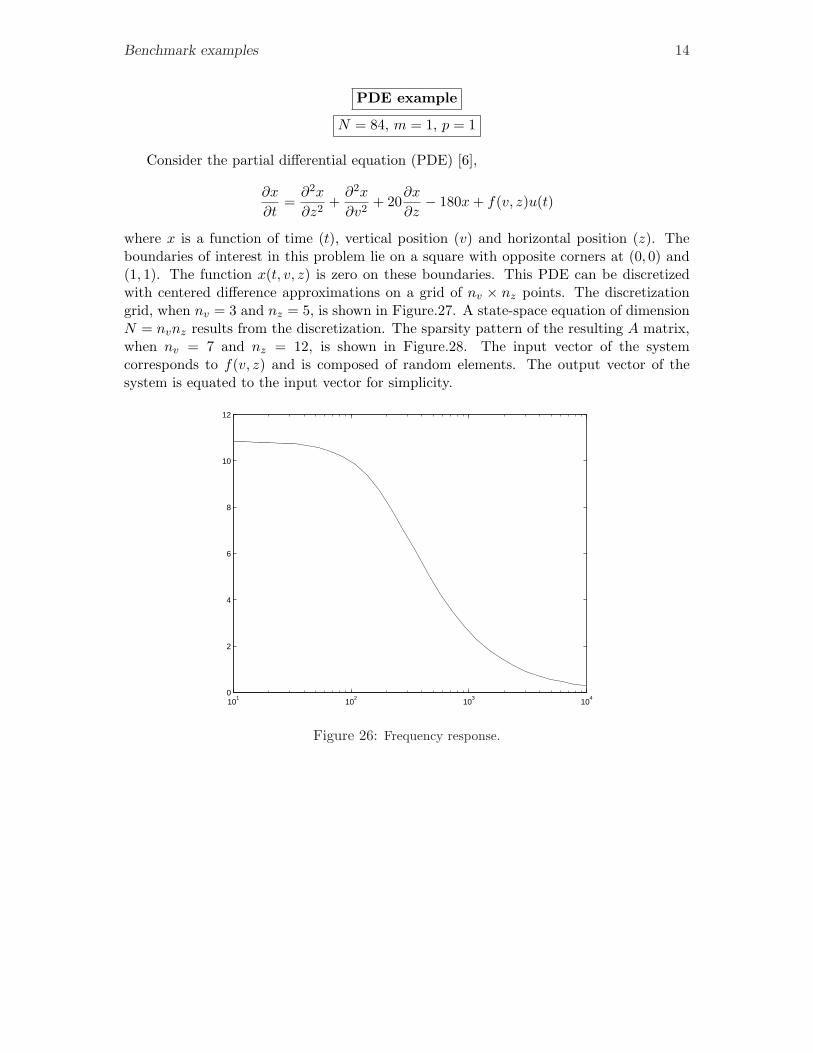
PDE example
N = 84, m = 1, p = 1
Consider the partial differential equation (PDE) [6],
∂x
∂t=
∂2x
∂z2+
∂2x
∂v2+ 20
∂x
∂z− 180x + f(v, z)u(t)
where x is a function of time (t), vertical position (v) and horizontal position (z). Theboundaries of interest in this problem lie on a square with opposite corners at (0, 0) and(1, 1). The function x(t, v, z) is zero on these boundaries. This PDE can be discretizedwith centered difference approximations on a grid of nv × nz points. The discretizationgrid, when nv = 3 and nz = 5, is shown in Figure.27. A state-space equation of dimensionN = nvnz results from the discretization. The sparsity pattern of the resulting A matrix,when nv = 7 and nz = 12, is shown in Figure.28. The input vector of the systemcorresponds to f(v, z) and is composed of random elements. The output vector of thesystem is equated to the input vector for simplicity.
101
102
103
104
0
2
4
6
8
10
12
Figure 26: Frequency response.

Benchmark examples 15
(0,0)
(1,1)
Figure 27: Discretization mesh, 3× 5 case.
0 10 20 30 40 50 60 70 80
0
10
20
30
40
50
60
70
80
row
colu
mn
Figure 28: Sparsity of A.
−1200 −900 −600 −300−80
−40
0
40
80
Figure 29: eigenvalue of A
0 21 42 63 8410
−20
10−15
10−10
10−5
100
Figure 30: . svd(Gc), o svd(Go), hsv
Benchmark examples 16
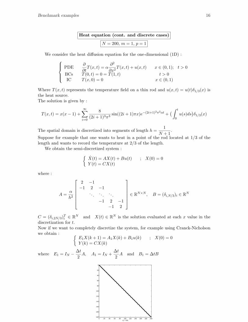
Heat equation (cont. and discrete cases)
N = 200, m = 1, p = 1
We consider the heat diffusion equation for the one-dimensional (1D) :
PDE∂
∂tT (x, t) = α
∂2
∂x2T (x, t) + u(x, t) x ∈ (0, 1); t > 0
BCs T (0, t) = 0 = T (1, t) t > 0IC T (x, 0) = 0 x ∈ (0, 1)
Where T (x, t) represents the temperature field on a thin rod and u(x, t) = u(t)δ1/3(x) isthe heat source.The solution is given by :
T (x, t) = x(x− 1) +∞∑
i=0
8(2i + 1)3π3
sin((2i + 1)πx)e−(2i+1)2π2αt +( ∫ t
0u(s)ds
)δ1/3(x)
The spatial domain is discretized into segments of length h =1
N + 1.
Suppose for example that one wants to heat in a point of the rod located at 1/3 of thelength and wants to record the temperature at 2/3 of the length.
We obtain the semi-discretized system :{
X(t) = AX(t) + Bu(t) ; X(0) = 0Y (t) = CX(t)
where :
A =α
h2
2 −1−1 2 −1
. . . . . . . . .−1 2 −1
−1 2
∈ RN×N , B = (δi,N/3)i ∈ RN
C = (δi,2N/3)Ti ∈ RN and X(t) ∈ RN is the solution evaluated at each x value in the
discretization for t.Now if we want to completely discretize the system, for example using Cranck-Nicholsonwe obtain : {
E1X(k + 1) = A1X(k) + B1u(k) ; X(0) = 0Y (k) = CX(k)
where E1 = IN − ∆t
2A, A1 = IN +
∆t
2A and B1 = ∆tB
0 20 40 60 80 100 120 140 160 180 200
0
20
40
60
80
100
120
140
160
180
200
nz = 598
Figure 31: sparsity A, A1 and E1

Benchmark examples 17
Continuous case
0 40 80 120 160 200−1800
−1400
−1000
−600
−200
Figure 32: Eigenvalues of A
Discretized case
0 20 40 60 80 100 120 140 160 180 200−1
−0.8
−0.6
−0.4
−0.2
0
0.2
0.4
0.6
0.8
1
Figure 33: Generalized eigenvalues of λE −A
0 20 40 60 80 100 120 140 160 180 20010
−25
10−20
10−15
10−10
10−5
100
Figure 34: .. svd(Gc), o svd(Go), x hsv
0 20 40 60 80 100 120 140 160 180 20010
−25
10−20
10−15
10−10
10−5
100
105
Figure 35: .. svd(Gc), o svd(Go), x hsv
10−2
10−1
100
101
102
103
104
10−20
10−18
10−16
10−14
10−12
10−10
10−8
10−6
10−4
10−2
100
Figure 36: frequency response
10−2
10−1
100
101
10−5
10−4
10−3
10−2
10−1
Figure 37: frequency response

Benchmark examples 18
Orr-Somerfeld example
N = 100, m = 1, p = 1
The Orr-Sommerfeld operator for Couette flow (the mean velocity varies as U = y, y isthe height) is in perturbation velocity variables [5]:
A = (−D2)12 D−2
(− ijkD2 +
1Re
D4)(−D2)−
12
where D = ddy and appropriate boundary conditions have been introduced (the pertur-
bation velocities vanish at the walls) so that the inverse operators are defined. Re is theReynolds number, and k is the x-wavenumber of the perturbation. This operator governsthe evolution of 2-dimensional perturbations.The matrix a 100 × 100 discretization for Reynolds number Re = 800 and k = 1 (thisdiscretization gives accurate results for this Reynolds number).
10−1
100
101
101
102
103
Figure 38: Frequency response.
0 25 50 75 100
10−1
100
101
102
103
Figure 39: . svd(Gc), o svd(Go), hsv
−10 −9 −8 −7 −6 −5 −4 −3 −2 −1 0−1
−0.8
−0.6
−0.4
−0.2
0
0.2
0.4
0.6
0.8
1
Figure 40: eigenvalues of A
Benchmark examples 19
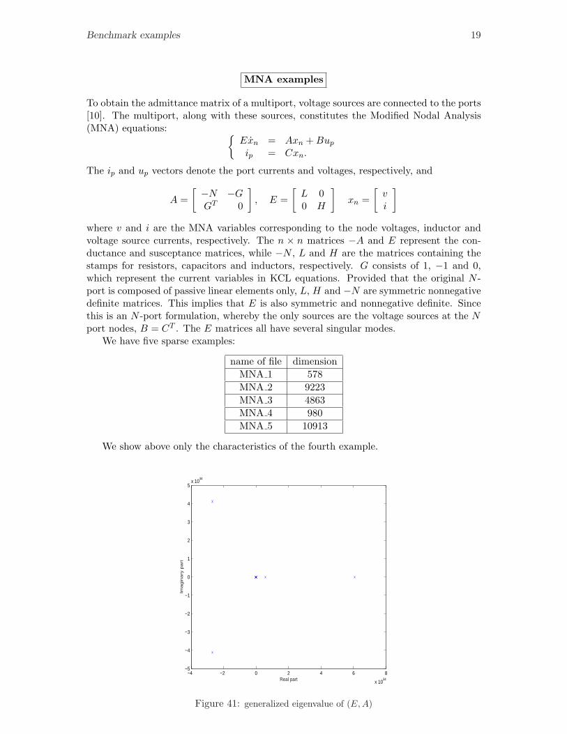
MNA examples
To obtain the admittance matrix of a multiport, voltage sources are connected to the ports[10]. The multiport, along with these sources, constitutes the Modified Nodal Analysis(MNA) equations: {
Exn = Axn + Bup
ip = Cxn.
The ip and up vectors denote the port currents and voltages, respectively, and
A =[ −N −G
GT 0
], E =
[L 00 H
]xn =
[vi
]
where v and i are the MNA variables corresponding to the node voltages, inductor andvoltage source currents, respectively. The n × n matrices −A and E represent the con-ductance and susceptance matrices, while −N , L and H are the matrices containing thestamps for resistors, capacitors and inductors, respectively. G consists of 1, −1 and 0,which represent the current variables in KCL equations. Provided that the original N -port is composed of passive linear elements only, L, H and −N are symmetric nonnegativedefinite matrices. This implies that E is also symmetric and nonnegative definite. Sincethis is an N -port formulation, whereby the only sources are the voltage sources at the Nport nodes, B = CT . The E matrices all have several singular modes.
We have five sparse examples:
name of file dimensionMNA 1 578MNA 2 9223MNA 3 4863MNA 4 980MNA 5 10913
We show above only the characteristics of the fourth example.
−4 −2 0 2 4 6 8
x 1034
−5
−4
−3
−2
−1
0
1
2
3
4
5x 10
34
Real part
Imagin
ary
part
Figure 41: generalized eigenvalue of (E, A)

Benchmark examples 20
0 100 200 300 400 500 600 700 800 900
0
100
200
300
400
500
600
700
800
900
nz = 83568
Figure 42: sparsity E
0 100 200 300 400 500 600 700 800 900
0
100
200
300
400
500
600
700
800
900
nz = 2872
Figure 43: sparsity A

Benchmark examples 21
International space station
N = 270, m = 3, p = 3
It is a structural model of component 1r (Russian service module) of the InternationalSpace Station (ISS) [1].
0 50 100 150 200 250
0
50
100
150
200
250
nz = 405
Figure 44: Sparsity of A.
−0.35 −0.3 −0.25 −0.2 −0.15 −0.1 −0.05 0−80
−60
−40
−20
0
20
40
60
80
Real part
Ima
gin
ary
pa
rt
Figure 45: Eigenvalues of A.
0 90 180 27010
−35
10−30
10−25
10−20
10−15
10−10
10−5
100
105
Figure 46: .. svd(Gc), o svd(Gc1),x svd(Gc2), + svd(Gc3), hsv
0 90 180 27010
−40
10−35
10−30
10−25
10−20
10−15
10−10
10−5
100
Figure 47: .. svd(Go), o svd(Go1),x svd(Go2), + svd(Go3), hsv

Benchmark examples 22
10−2
10−1
100
101
102
103
10−6
10−5
10−4
10−3
10−2
10−1
100
1st input / 1st output
frequency (rad/sec)
ab
s(g
(j.w
))
10−2
10−1
100
101
102
103
10−9
10−8
10−7
10−6
10−5
10−4
1st input / 2nd output
frequency (rad/sec)
ab
s(g
(j.w
))10
−210
−110
010
110
210
310
−8
10−7
10−6
10−5
10−4
10−3
10−2
1st input / 3d output
frequency (rad/sec)
ab
s(g
(j.w
))
10−2
10−1
100
101
102
103
10−9
10−8
10−7
10−6
10−5
10−4
frequency (rad/sec)
ab
s(g
(j.w
))
2nd input / 1st output
10−2
10−1
100
101
102
103
10−7
10−6
10−5
10−4
10−3
10−2
10−1
frequency (rad/sec)
ab
s(g
(j.w
))
2nd input / 2nd output
10−2
10−1
100
101
102
103
10−11
10−10
10−9
10−8
10−7
10−6
10−5
10−4
10−3
frequency (rad/sec)
ab
s(g
(j.w
))
2nd input / 3d output
10−2
10−1
100
101
102
103
10−7
10−6
10−5
10−4
10−3
10−2
frequency (rad/sec)
ab
s(g
(j.w
))
3d input / 1st output
10−2
10−1
100
101
102
103
10−7
10−6
10−5
10−4
10−3
10−2
frequency (rad/sec)
ab
s(g
(j.w
))
3d input / 3d output
10−2
10−1
100
101
102
103
10−10
10−9
10−8
10−7
10−6
10−5
10−4
10−3
frequency (rad/sec)
ab
s(g
(j.w
))
3d input / 2nd output
Figure 48: Frequency response of the ISS model.
Benchmark examples 23
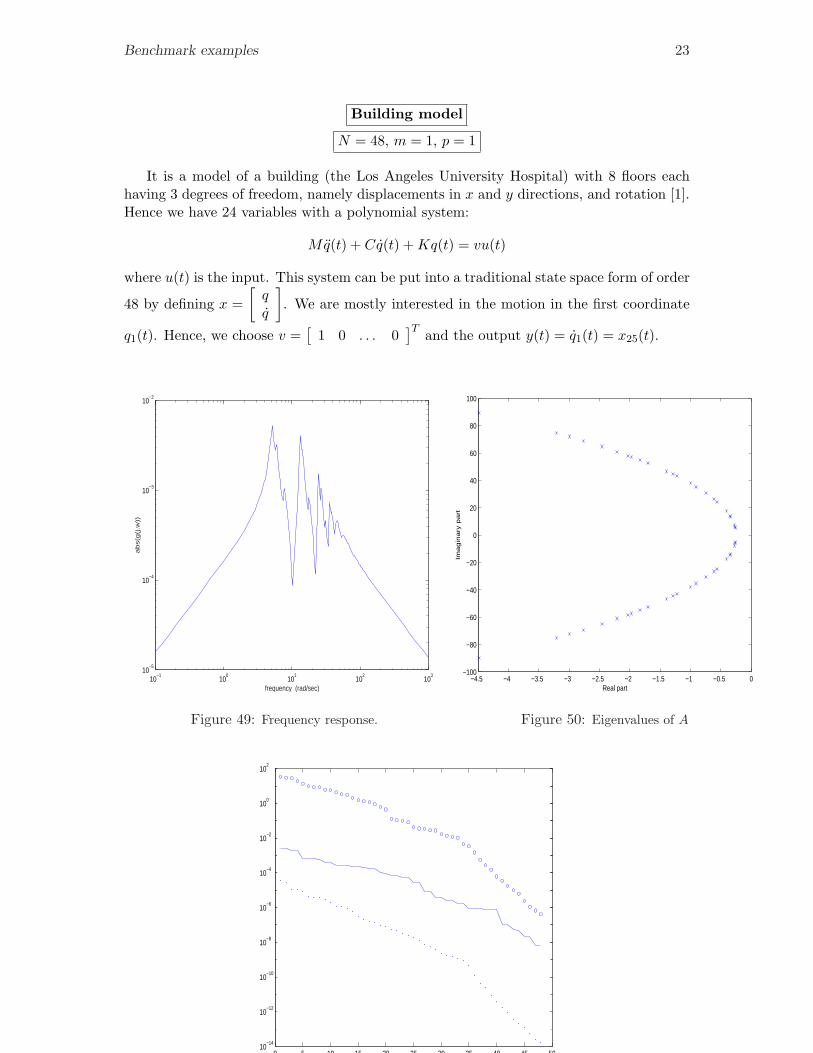
Building model
N = 48, m = 1, p = 1
It is a model of a building (the Los Angeles University Hospital) with 8 floors eachhaving 3 degrees of freedom, namely displacements in x and y directions, and rotation [1].Hence we have 24 variables with a polynomial system:
Mq(t) + Cq(t) + Kq(t) = vu(t)
where u(t) is the input. This system can be put into a traditional state space form of order
48 by defining x =[
]. We are mostly interested in the motion in the first coordinate
q1(t). Hence, we choose v =[
1 0 . . . 0]T and the output y(t) = q1(t) = x25(t).
10−1
100
101
102
103
10−5
10−4
10−3
10−2
frequency (rad/sec)
ab
s(g
(j.w
))
Figure 49: Frequency response.
−4.5 −4 −3.5 −3 −2.5 −2 −1.5 −1 −0.5 0−100
−80
−60
−40
−20
0
20
40
60
80
100
Real part
Ima
gin
ary
pa
rt
Figure 50: Eigenvalues of A
0 5 10 15 20 25 30 35 40 45 5010
−14
10−12
10−10
10−8
10−6
10−4
10−2
100
102
Figure 51: .. svd(Gc), o svd(Go),hsv

Benchmark examples 24
Clamped beam model
N = 348, m = 1, p = 1
The clamped beam model has 348 states, it is obtained by spatial discretization of anappropriate partial differential equation [1]. The input represents the force applied to thestructure at the free end, and the output is the resulting displacement.
10−2
10−1
100
101
102
103
104
10−5
10−4
10−3
10−2
10−1
100
101
102
103
104
frequency (rad/sec)
ab
s(g
(j.w
))
Figure 52: Frequency response.
−600 −500 −400 −300 −200 −100 0−100
−80
−60
−40
−20
0
20
40
60
80
100
Real part
Ima
gin
ary
pa
rt
Figure 53: Eigenvalues of A
0 50 100 150 200 250 300 35010
−35
10−30
10−25
10−20
10−15
10−10
10−5
100
105
1010
Figure 54: .. svd(Gc), o svd(Go),hsv

Bibliographie 25
Acknowledgement
We would like to thank T. Antoulas, S. Gugercin, B. Farrell, P. Ioannou and J. R. Li forcontributing some of the examples.
References
[1] A. C. Antoulas, D. C. Sorenson and S. Gugercin, ” A Survey of Model ReductionMethods for Large-Scale Systems”, Contemporary Mathematics, 280, pp.193–219,2001.
[2] E. Chiprout and M. S. Nakhla, ”Asymptotic Waveform Evaluation and MomentMatching for Interconnect Analysis”, Boston, MA : Kluwer Academic Publishers,1994.
[3] Y. Chahlaoui, D. Lemonnier, K. Meerbergen, A. Vandendorpe and P. Van Dooren,”Model Reduction of Second Order Systems”, accepted to MTNS2002.
[4] W. Draijer, M. Steinbuch and O. H. Bosgra, ”Adaptive Control of the Radial ServoSystem of a Compact Disc Player”, IFAC Automatica, vol 28, no.3, pp.455–462, 1992.
[5] B. F. Farrell and P. J.Ioannou, ”Accurate Low Dimensional Approximation of theLinear Dynamics of Fluid Flow”, American Meteorological Society, pp. 2771–2789,2001.
[6] E. J. Grimme, ”Krylov Projection Methods for Model Reduction”, Ph. D in theGraduate College of the University of Illinois at Urbana-Champaign, 1997
[7] H. Heeb, A. E. Ruehli, J. E. Bracken, and R. A. Rohrer, ”Three Dimensional CircuitOriented Electromagnetic Modeling for VLSI Interconnects”, Proc. IEEE Int. Conf.Computer Design, Cambridge, MA, pp. 218–221, 1992.
[8] J. R. Li and J. White, ”Efficient Model Reduction of Interconnect via Approxi-mate System Gramians”, Proceedings of the IEEE/ACM International Conferenceon Computer-Aided Design, pp.380–383, 1999.
[9] N. Marques, M. Kamon, J. White and L. M. Silveira, ”A Mixed Nodal-Mesh For-mulation for Efficient Extraction and Passive Reduced-Order Modeling of 3D Inter-connects”, Proceedings of the 35th IEEE/ACM Design Automation Conference,SanFransisco, CA, pp.297–302, 1998.
[10] A. Odabasioglu, M. Celik and L. T. Pileggi, ”PRIMA: Passive Reduced-order Inter-connect Macromodeling Algorithm”, IEEE Transactions on Computer-Aided Designof Integrated Circuits and Systems, vol.17, no.8, pp.645–654, 1998.
[11] T. Penzl, ”Algorithms for Model Reduction of Large Dynamical Systems”, TRSFB393/99-40, Sonderforschungsbereich 393 Numerische Simulation auf massiv par-allel Rechern, TU Chemnitz, 09107, FRG, 1999.
[12] Y. Saad, ”Projection and Deflation Methods for Partial Pole Assignment in LinearState Feedback”, IEEE Trans. Autom. Control, vol.33, pp.290–297, 1988.

Bibliographie 26
[13] P. M. R. Wortelboer, M. Steinbuch and O. H. Bosgra, ”Closed-Loop Balanced Re-duction with Application to a Compact Disc Mechanism”, Selected Topics in Identi-fication, Modeling and Control, vol.9, Delft University Press, December 1996.