a case study of co-induction in isabelle 1 · a case study of co-induction in isabelle 1 jacob...

A Case Study of Co-induction in Isabelle 1

Jacob FrostComputer Laboratory

University of Cambridgee-mail:[email protected]

February 1995

1Supported by ESPRIT Basic Research Project 6453, Types for Proofs and Pro-grams and the Danish Natural Science Research Council

Abstract

The consistency of the dynamic and static semantics for a small functional pro-gramming language was informally proved by R.Milner and M.Tofte. The notionsof co-inductive definitions and the associated principle of co-induction played apivotal role in the proof. With emphasis on co-induction, the work presented heredeals with the formalisation of this result in the generic theorem prover Isabelle.

Contents

1 Introduction 1

2 Co-induction in Relation Semantics 22.1 Notation . . . . . . . . . . . . . . . . . . . . . . . . . . . . . . . . 22.2 The Language . . . . . . . . . . . . . . . . . . . . . . . . . . . . . 22.3 Dynamic Semantics . . . . . . . . . . . . . . . . . . . . . . . . . . 32.4 Static Semantics . . . . . . . . . . . . . . . . . . . . . . . . . . . 32.5 Consistency . . . . . . . . . . . . . . . . . . . . . . . . . . . . . . 5

3 Isabelle 73.1 Documentation . . . . . . . . . . . . . . . . . . . . . . . . . . . . 73.2 Notation . . . . . . . . . . . . . . . . . . . . . . . . . . . . . . . . 73.3 Typed Lambda Calculus . . . . . . . . . . . . . . . . . . . . . . . 73.4 Pure Isabelle . . . . . . . . . . . . . . . . . . . . . . . . . . . . . 8

3.4.1 Syntax . . . . . . . . . . . . . . . . . . . . . . . . . . . . . 83.4.2 Inferences . . . . . . . . . . . . . . . . . . . . . . . . . . . 83.4.3 Proofs . . . . . . . . . . . . . . . . . . . . . . . . . . . . . 93.4.4 Tactics and Tacticals . . . . . . . . . . . . . . . . . . . . . 9

3.5 Higher Order Logic . . . . . . . . . . . . . . . . . . . . . . . . . . 93.5.1 Basic HOL . . . . . . . . . . . . . . . . . . . . . . . . . . . 103.5.2 HOL Set Theory . . . . . . . . . . . . . . . . . . . . . . . 103.5.3 (Co)Inductive definitions in HOL . . . . . . . . . . . . . . 11

3.6 Zermelo-Frankel Set Theory . . . . . . . . . . . . . . . . . . . . . 123.6.1 Basic ZF . . . . . . . . . . . . . . . . . . . . . . . . . . . . 123.6.2 (Co)Inductive definitions in ZF . . . . . . . . . . . . . . . 14

4 Formalisation in Isabelle HOL 144.1 A theory Least and Greatest Fixed Points . . . . . . . . . . . . . 144.2 The Language . . . . . . . . . . . . . . . . . . . . . . . . . . . . . 174.3 Dynamic Semantics . . . . . . . . . . . . . . . . . . . . . . . . . . 174.4 Static Semantics . . . . . . . . . . . . . . . . . . . . . . . . . . . 214.5 Consistency . . . . . . . . . . . . . . . . . . . . . . . . . . . . . . 24

4.5.1 Stating Consistency . . . . . . . . . . . . . . . . . . . . . . 244.5.2 Proving Consistency . . . . . . . . . . . . . . . . . . . . . 26

4.6 Discussion . . . . . . . . . . . . . . . . . . . . . . . . . . . . . . . 294.6.1 Inductive and Co-inductive Definitions . . . . . . . . . . . 294.6.2 Avoiding Co-induction . . . . . . . . . . . . . . . . . . . . 294.6.3 Working with Isabelle HOL . . . . . . . . . . . . . . . . . 30

i

5 Formalisation in Isabelle ZF 305.1 The Language . . . . . . . . . . . . . . . . . . . . . . . . . . . . . 315.2 Dynamic Semantics . . . . . . . . . . . . . . . . . . . . . . . . . . 32

5.2.1 Variant Maps . . . . . . . . . . . . . . . . . . . . . . . . . 325.2.2 Values and Value Environments . . . . . . . . . . . . . . . 355.2.3 Evaluation . . . . . . . . . . . . . . . . . . . . . . . . . . . 37

5.3 Static Semantics . . . . . . . . . . . . . . . . . . . . . . . . . . . 375.3.1 Types and Type Environments . . . . . . . . . . . . . . . 395.3.2 Basic Correspondence Relation . . . . . . . . . . . . . . . 395.3.3 Elaboration . . . . . . . . . . . . . . . . . . . . . . . . . . 39

5.4 Consistency . . . . . . . . . . . . . . . . . . . . . . . . . . . . . . 415.4.1 Stating Consistency . . . . . . . . . . . . . . . . . . . . . . 415.4.2 Proving Consistency . . . . . . . . . . . . . . . . . . . . . 44

5.5 Discussion . . . . . . . . . . . . . . . . . . . . . . . . . . . . . . . 455.5.1 Non-well-founded objects in ZF . . . . . . . . . . . . . . . 455.5.2 The (co)inductive package . . . . . . . . . . . . . . . . . . 45

6 Conclusion 46

ii

List of Figures

1 Constants, variables and expressions . . . . . . . . . . . . . . . . 22 Values, environments, closures, ... . . . . . . . . . . . . . . . . . . 33 Evaluation . . . . . . . . . . . . . . . . . . . . . . . . . . . . . . . 44 Type constants, types, type environments, ... . . . . . . . . . . . . 45 Elaboration . . . . . . . . . . . . . . . . . . . . . . . . . . . . . . 56 Consistency . . . . . . . . . . . . . . . . . . . . . . . . . . . . . . 57 Extended correspondence relation . . . . . . . . . . . . . . . . . . 68 Greatest fixed points and co-induction . . . . . . . . . . . . . . . 69 Meta-level connectives . . . . . . . . . . . . . . . . . . . . . . . . 810 Logical symbols in HOL . . . . . . . . . . . . . . . . . . . . . . . 1011 Symbols in HOL set theory . . . . . . . . . . . . . . . . . . . . . 1112 Logical symbols in ZF . . . . . . . . . . . . . . . . . . . . . . . . 1213 Symbols in ZF . . . . . . . . . . . . . . . . . . . . . . . . . . . . . 1314 Least and greatest fixed points in HOL . . . . . . . . . . . . . . . 1415 Properties of least and greatest fixed points in HOL . . . . . . . . 1516 Properties of least and greatest fixed points in HOL . . . . . . . . 1617 Properties of least and greatest fixed points in HOL . . . . . . . . 1618 Constants, variables and expressions in HOL . . . . . . . . . . . . 1819 Values, value environments and closures in HOL . . . . . . . . . . 1920 Evaluation in HOL . . . . . . . . . . . . . . . . . . . . . . . . . . 2021 Properties of evaluation in HOL . . . . . . . . . . . . . . . . . . . 2222 Type constants, types and type environments in HOL . . . . . . . 2323 Basic correspondence relation in HOL . . . . . . . . . . . . . . . . 2424 Elaboration in HOL . . . . . . . . . . . . . . . . . . . . . . . . . . 2525 Properties of elaboration in HOL . . . . . . . . . . . . . . . . . . 2626 Extended correspondence relation in HOL . . . . . . . . . . . . . 2727 Co-induction rules for hasty rel in HOL . . . . . . . . . . . . . 2828 Consistency in HOL . . . . . . . . . . . . . . . . . . . . . . . . . 2829 Constants, variables and expressions in ZF . . . . . . . . . . . . . 3130 Variant maps in ZF . . . . . . . . . . . . . . . . . . . . . . . . . . 3431 Values and value environments in ZF . . . . . . . . . . . . . . . . 3632 Evaluation in ZF . . . . . . . . . . . . . . . . . . . . . . . . . . . 3833 Type constants, types and type environments in ZF . . . . . . . . 4034 Basic correspondence relation in ZF . . . . . . . . . . . . . . . . . 4135 Elaboration in ZF . . . . . . . . . . . . . . . . . . . . . . . . . . . 4236 Extented correspondence relation in ZF . . . . . . . . . . . . . . . 4337 Consistency in ZF . . . . . . . . . . . . . . . . . . . . . . . . . . . 44

iii

1 Introduction

In the paper Co-induction in Relational Semantics [2], R.Milner and M.Tofteprove the dynamic and static semantics for a small functional programming lan-guage consistent. The dynamic semantics associates a value to an expression ofthe language, while the static semantics associates a type. A value has a type.Consistency requires that the value of an expression has the type of the expres-sion. Values can be infinite or non-well-founded because the language containsrecursive functions. Non-well-founded values are handled using co-inductive def-initions and the corresponding proof principle of co-induction. The notion ofgreatest fixed points are used to deal with co-inductive definitions. The aim oftheir paper is to direct attention to the principle of co-induction, by giving anexample of its application to computer science.

The purpose of this paper is to investigate how the same consistency resultcan be proved formally in the generic theorem prover Isabelle. There is littledoubt that it is possible to prove the same or at least a very similar result inIsabelle. A more interesting question is how easy and natural this can be done,in particular how well Isabelle can handle the notions of co-inductive definitionsand co-induction. To answer the above question, and thereby unveiling strongand weak points of the Isabelle system, is therefore also a purpose of this paper.

In order to come up with an answer, this paper describes the formalisationof the consistency result in two of Isabelles object logics: Higher Order Logic(HOL) and Zermelo-Frankel Set Theory (ZF). Throughout this paper, the formaltreatments will be compared to each other and to their more informal counterpart.The formal development in HOL and ZF was carried out with more than one yearin between. The comparison should therefore not only illustrate differences andsimilarities between formal/informal treatment, the object logics ZF/HOL, butalso how Isabelle have evolved in that year.

This paper is an extension of an earlier paper [1] only describing the formal-isation of the consistency result in Isabelle HOL. As its predecessor, this paperis meant to be largely self contained. As a consequence a survey of the originalpaper [2] by Robin Milner and Mads Tofte is given first. For the same reason,it is followed by an overview of the Isabelle system and its implementation ofHOL and ZF. In the following two sections the formalisation in Isabelle HOL andIsabelle ZF is discussed. Finally a few conclusions. The sections describing theoriginal paper [2] and the formalisation in HOL are kept almost unchanged fromthe first paper. The overview of Isabelle is extended to describe the implemen-tation of ZF. The section on the formalisation in ZF is new and the conclusionis changed to reflect the extra information obtained.

1

2 Co-induction in Relation Semantics

The aim of this section, is to give an overview of the parts of the paper [2] thatmust be formalised in order to prove the consistency result. For a more thoroughtreatment please refer to the original paper [2].

The original paper is concerned with proving the consistency of the dynamicand static semantics of a small functional programming language. As a conse-quence it first defines such a language. Then it defines the dynamic semantics,which associates values to expressions and the static semantics which associatestypes to expressions. Finally it states and proves consistency.

The first part of this section is concerned with notation. After that the restof this section will follow the structure of the original paper.

2.1 Notation

The notation used here is quite similar to that of the original paper. It differsslightly in order to make the notation of this paper more homogeneous.

Let A and B be two sets. In the following, the disjoint union is written A+B

and the set of finite maps from A to B as Afin−→ B. A finite map is written on

the form {a1 7→ b1, . . . , an 7→ bn}. For f ∈ A fin−→ B, dom(f) denotes the domain

and rng(f) the range of the map. If f, g ∈ A fin−→ B then f + g means f modifiedby g.

2.2 The Language

The language of expressions is defined by the BNF shown in Figure 1. Thereare five different kinds of expressions: constants including constant functions,variables, abstractions, recursive functions and applications.

c ∈ Constv ∈ Vare ∈ Ex ::= Const | Var | fn Var⇒ Ex | fix Var(Var) = Ex | Ex Ex

Figure 1: Constants, variables and expressions

A key point here, is the existence of recursive functions. Without those therewould be no need for non-well-founded values and consequently no need for co-induction in the proof of consistency.

2

2.3 Dynamic Semantics

An expression evaluates to a value in some environment. The purpose of thedynamic semantics is to relate environments and expressions to values. The firsttask is therefore to explain the notions of environments and values. Furthermoreit must be explained how constant functions are applied to constants.

v ∈ Val = Const + Clos (1)

ve ∈ ValEnv = Varfin−→ Val (2)

cl or 〈x, e, ve〉 ∈ Clos = Var× Ex× ValEnv (3)Exists unique cl∞ solving: cl∞ = 〈x, e, ve+ {f 7→ cl∞}〉 (4)

apply ∈ Const× Const→ Const (5)

Figure 2: Values, environments, closures, ...

Values (1) are either constants or closures. Constant expressions always evalu-ate to constant values, while abstractions and recursively defined functions alwaysevaluate to closures. Applications can evaluate to either. Environments (2) mapsvariables to values. Closures (3) represent functions and are triples consisting ofthe parameter to the function, the function body and the environment in whichthe body should be evaluated. Closures can be infinite or non-well-founded dueto the existence of recursive functions. In case of a recursive function, the envi-ronment of the closure will map the name of the function to the closure itself.The requirement (4) expresses that the three mutual recursive equations (1)-(3) must be solved such that the set of closures contains the non-well-foundedclosures. Finally, the function apply (5) is supposed to capture how constantfunctions are applied to constants.

The dynamic semantics is a relational semantics often called a natural seman-tics. It is formulated as an inference system consisting of six rules. All the ruleshave conclusions of the form ve ` e −→ v, read e evaluates to v in ve. Theinference system appears in Figure 3.

It is worth noting that the only purpose of (4) is to ensure that the dynamicsemantics always relates a unique value to a recursive function. It is never useddirectly in the proof of consistency.

2.4 Static Semantics

An expression elaborates to a type in some type environment. The purpose of thestatic semantics is to relate type environments and expressions to types. Beforethis can be done, the notion of type and type environments must be explained.It must also be explained what type a constant has.

3

ve ` c −→ c

x ∈ dom(ve)ve ` x −→ ve(x)

ve ` fn x⇒ e −→ 〈x, e, ve〉

cl∞ = 〈x, e, ve+ {f 7→ cl∞}〉ve ` fix f(x) = e −→ cl∞

ve ` e1 −→ c1 ve ` e2 −→ c2 c = apply(c1, c2)ve ` e1 e2 −→ c

ve ` e1 −→ 〈x′, e′, ve′〉ve ` e2 −→ v2

ve′ + {x′ 7→ v2} ` e′ −→ vve ` e1 e2 −→ v

Figure 3: Evaluation

τ ∈ Ty ::= {int, bool, . . .} | Ty→ Ty (6)

te ∈ TyEnv = Varfin−→ Ty (7)

isof ⊆ Const× Ty (8)If c1 isof τ1 → τ2 and c2 isof τ1 then apply(c1, c2) isof τ2 (9)

Figure 4: Type constants, types, type environments, ...

Types are primitive types, such as int, bool or function types (6). Typeenvironments map variables to types (7). The correspondence relation isof (8)relate a constant to its type. The idea is that it should relate for example 3 to intand true to bool. It must be consistent with the function apply (9). The relationisof is extended pointwise to relate environments and type environments.

The static semantics is again a relational semantics, formulated as an inferencesystem and consisting of five rules. All the rules have conclusions of the formte ` e =⇒ τ , read e elaborates to τ in te. The inference system is shown inFigure 5.

4

c isof τte ` c =⇒ τ

x ∈ dom(te)te ` x =⇒ te(x)

te+ {x 7→ τ1} ` e =⇒ τ2

te ` fn x⇒ e =⇒ τ1 → τ2

te+ {f 7→ τ1 → τ2}+ {x 7→ τ1} ` e =⇒ τ2

te ` fix f(x) = e =⇒ τ1 → τ2

te ` e1 =⇒ τ1 → τ2 te ` e2 =⇒ τ1

te ` e1 e2 =⇒ τ2

Figure 5: Elaboration

2.5 Consistency

The original paper is concerned with proving what is called basic consistency(10). Basic consistency expresses that in corresponding environments, expressionsevaluating to constants must elaborate to the type of the constant. At first itmight seem strange only to consider constant values. The reason is that functions,represented as closures, only are of interest because they can be applied and inthe end yield some constant value.

Basic consistency cannot be proved directly by induction on the structureof evaluations. The reason is that an evaluation resulting in a constant mightrequire evaluations resulting in closures. Attempting to do a proof, it manifestitself as too weak induction hypothesises.

Basic Consistency

If ve isof te and ve ` e −→ c and te ` e =⇒ τ then c isof τ (10)

Consistency

If ve : te and ve ` e −→ v and te ` e =⇒ τ then v : τ (11)

Figure 6: Consistency

It is necessary to prove a stronger result, called consistency (11). Consistencyis formulated by extending the correspondence relation isof. The extended cor-respondence relation, :, also expresses what it means for a closure to have a type.

5

It is defined as the greatest fixed point of the function in Figure 7. See [2] for adiscussion of why this particular function was chosen.

f(s) ≡ { 〈v, τ〉 |if v = c then c isof τ ;if v = 〈x, e, ve〉then there exist a te such that

te ` fn x⇒ e =⇒ τ anddom(ve) = dom(te) and〈ve(x), te(x)〉 ∈ s for all x ∈ dom(ve)

}v : τ ≡ 〈v, τ〉 ∈ gfp(Val× Ty, f)

Figure 7: Extended correspondence relation

The notion of greatest fixed point is defined in Figure 8. The correspondingprinciple of co-induction expresses, that in order to prove that a set s is includedin the greatest fixed point of some function f , it is enough to prove that it isf -consistent, i.e. s ⊆ f(s).

Greatest Fixed Points

gfp(u, f) ≡ ⋃{s ⊆ u | s ⊆ f(s)}

Co-induction

s ⊆ f(s)s ⊆ gfp(u, f)

Figure 8: Greatest fixed points and co-induction

It is interesting to consider what would happen if : was defined using the leastfixed point instead of the greatest. The function f does not require non-well-founded closures to be related to types. As a consequence taking the least fixedpoint, only the well-founded closures would be related to types. This would makeit impossible to prove the result because closures might be non-well-founded. Onthe other hand, the function does not prevent non-well-founded closure frombeing related to types. Therefore taking the greatest fixed point causes non-well-founded closures to be related as well.

Consistency is proved by induction on the structure of evaluations or as theyexpressed in [2], on the depth of the inference. Applying induction, results in sixcases, one for each of the rules of the dynamic semantics. The case for recursive

6

functions is the most interesting in that it uses co-induction. The reason is thatthe non-well-founded closures are introduced by recursive functions.

3 Isabelle

Isabelle is a generic theorem prover. It can be instantiated to support reasoningin an object-logic by extending its meta-logic. All the symbols of the object-logicare declared using typed lambda calculus, while the rules are expressed as axiomsin the meta-logic.

This section attempt to give an overview over Isabelle. At first, a briefoverview of the Isabelle documentation is given. Then the notation is explained,followed by a description of the typed lambda calculus used by Isabelle. Nextthe pure Isabelle system is described and it is explained how the pure Isabellesystem is extended to support reasoning in HOL and ZF.

3.1 Documentation

The Isabelle system is extensively documented. The main reference is the Is-abelle Book [8]. This book contains most the information found in the threetechnical reports [9, 5, 4]. References will only be made to these reports if theinformation cannot be found in the Isabelle book. A number of other papers andreports discuss Isabelle and related issues and will be mentioned when necessary.Some information can only be found online in which case a URL address will beprovided.

3.2 Notation

Here and in the rest of the paper, an Isabelle-like notation will be used. TheIsabelle system uses an ASCII-notation. When working in Isabelle it is often nec-essary to supply information about the syntax, such as where arguments shouldbe placed when using mix-fix notation, precedence etc. In order to improve read-ability most such information is left out here and a more mathematical notationis adapted, allowing the use of mathematical symbols etc.

3.3 Typed Lambda Calculus

Isabelle represents syntax using the typed λ-calculus. Lambda abstraction iswritten λx.t and application t1(t2), where x is a variable and t, t1, t2 are terms.

Types in Isabelle can be polymorphic, ie. contain type variables such as α inthe type α list. Function types are written σ1 ⇒ σ2, where σ1 and σ2 are types.New constants are declared by giving their type, for example: succ :: nat⇒ nat.

7

Isabelle uses a notion of classes to control polymorphism. Each type belongto a class. A class can be a subset of another class. Isabelle contains the built-inclass logic of logical types. A new class is declared as a subclass of another class,for example the class term of terms which is included in the class logic. Newtypes and type constructors can be declared by giving the class of the argumentsand the result, for example list :: (term)term.

Curried abstraction λx1. . . . λxn.t is abbreviated λx1 . . . xn.t, and curried ap-plication t(t1) . . . (tn) as t(t1, . . . , tn). Similar curried function types σ1 ⇒(. . . σn ⇒ σ . . .) are abbreviated [σ1, . . . , σn]⇒ σ.

3.4 Pure Isabelle

Object-logics are implemented by extending pure Isabelle which is described here.Pure Isabelle consist of the meta-logic and has support for doing proofs in thismeta-logic and its possible extensions.

3.4.1 Syntax

Isabelle’s meta-logic is a fragment of intuitionistic higher order logic. The symbolsof the meta-logic is declared exactly the same way as symbols of an object-logic, by using typed lambda calculus. There is a built-in subclass of logic

called prop of meta-level truth values. The symbols of the meta-logic are thethree connectives, shown in Figure 9, corresponding to implication, universalquantification and equality.

Infixes

=⇒ :: [prop, prop]⇒ prop∧:: (α :: logic⇒ prop)⇒ prop

≡ :: [α :: logic, α]⇒ prop

Figure 9: Meta-level connectives

Nested implication φ1 =⇒ (. . . φn =⇒ φ . . .) may be abbreviated[[φ1; . . . ;φn]] =⇒ φ and outer quantifiers can be dropped.

3.4.2 Inferences

The meta-logic is defined by a set of primitive axioms and inference rules. Proofsare seldom constructed using these rules. Usually a derived rule, the resolutionrule, is used:

[[ψ1; . . . ;ψm]] =⇒ ψ [[φ1; . . . ;φn]] =⇒ φ([[φ1; . . . ;φi−1;ψ1; . . . ψm;φi+1; . . . ;φn]] =⇒ φ)s

(ψs ≡ φis)

8

Here 1 ≤ i ≤ n and s is a higher order unifier of ψ and φ. A big machinery isconnected with resolution and higher order unification. This includes schematicvariables, lifting over formulae and variables etc. For the details refer to [8].

3.4.3 Proofs

It is possible to construct proofs both in a forward and backward fashion inIsabelle. Bigger proofs are however usually constructed backwards.

In Isabelle, a backwards proof is done by refining a proof state, until thedesired result is proved. A proof state is simply a meta-level theorem of the form[[φ1; . . . ;φn]] =⇒ φ, where φ1, . . . , φn can be seen as subgoals and φ as the maingoal. Repeatedly refining such a proof state, by resolving it with suitable rules,corresponds to applying rules to the subgoals until they all are proved.

In order to manage backward proofs, Isabelle has a subgoal module. It keepstrack of the current and previous proof states. This make it possible, for example,to undo proof steps.

3.4.4 Tactics and Tacticals

Tactics perform backward proofs. They are applied to a proof state and maychange several of the subgoals.

Isabelle has many different tactics. There are tactics for proving a subgoalby assumption, different forms of resolution for applying rules to subgoals etc.These will work in all logics.

Isabelle also have a number of generic packages, which depend on propertiesof the logic in question. To mention two, a classical reasoning package and asimplifier package. Each contain a number of tactics. To get access to these, thepackages must be successfully instantiated for the actual logic. Then the classicalreasoning package, for example, will provide a suite of tactics for doing proofs,using classical proof procedures. The tactic fast tac for example will try tosolve a subgoal, by applying the rules in a supplied set of rules in a depth firstmanner.

Tactics can be combined to new tactics using tacticals. There are tacticals fordoing depth-first, best-first search etc., but also simpler tacticals for sequentialcomposition, choice, repetition etc.

3.5 Higher Order Logic

A number of logics have been implemented in Isabelle. Among these is HOL.The description of HOL given here will be brief and only cover parts relevant tothe rest of the presentation. For a thorough treatment refer to [8].

9

Prefixes

¬ :: bool⇒ bool negation

Infixes

= :: [α, α]⇒ bool equality∧ :: [bool, bool]⇒ bool conjunction∨ :: [bool, bool]⇒ bool disjunction→ :: [bool, bool]⇒ bool implication

Binders

∀ :: [α⇒ bool]⇒ bool universal quantification∃ :: [α⇒ bool]⇒ bool existential quantification

Translations

a 6= b ≡ ¬(a = b) not equal

Figure 10: Logical symbols in HOL

3.5.1 Basic HOL

There is a subclass of logic, called term of higher order terms and a type be-longing to this, bool of object-level truth values. There is an implicit coercion tometa-level truth values called Trueprop. The connectives needed for this paperis declared in Figure 10.

The formulation of HOL in Isabelle, identifies meta-level and object-leveltypes. This makes it possible to take advantage of Isabelle’s type system. Typechecking is done automatically and most type constraints are implicit.

Using Isabelle HOL one often wants to define new types. Isabelle does notsupport type definitions, but they can be mimicked by explicit definition of iso-morphism functions. See [3].

The meaning of the symbols is defined by a number of rules. They are usuallyformulated as introduction or elimination rules. Taking ∨ as an example, one ofits introduction rules is P =⇒ P ∨ Q and the elimination rule is [[P ∨ Q;P =⇒R;Q =⇒ R]] =⇒ R.

Most of the generic reasoning packages are instantiated to support reasoningin HOL. This includes the simplifier and the classical reasoning package.

3.5.2 HOL Set Theory

A formulation of set theory has been given within Isabelle HOL. Again only therelevant part of the theory is covered here, but a detailed description of the full

10

Types

set :: (term)term

Constants

({ }) :: α⇒ α set singleton

Binders

({ . }) :: [α⇒ bool]⇒ α set comprehension

Infixes

∈:: [α, α set]⇒ bool membership∪ :: [α set, α set]⇒ α set union∩ :: [α set, α set]⇒ α set intersection

Prefixes⋃:: ((α set) set)⇒ α set general union⋂:: ((α set) set)⇒ α set general intersection

Figure 11: Symbols in HOL set theory

theory can be found in [8].In order to formulate the set theory a new type constructor set is declared.

Then the symbols of the set theory are declared. The symbols necessary for thispresentation are shown in Figure 11.

Just as before the meaning of the symbols is defined by a number of rules.The set theory also contains a large number of derived rules. Most of the genericreasoning packages are also instantiated to support reasoning in the set theory.

The set theory is used to define a number of new types and type constructors,using the technique described in [3]. Examples include natural numbers nat,disjoint unions + and products ∗.

3.5.3 (Co)Inductive definitions in HOL

A package for doing inductive and co-inductive definitions has been developedin Isabelle HOL [10, 9]. Unfortunately this package was not available whenthe consistency proof by Mads Tofte and Robin Milner was formalised in HOL.Instead a basic theory of least and greatest fixed points was used. A descriptioncan be found in §4.1 and [3].

11

Prefixes

¬ :: o⇒ o negation

Infixes

= :: [α, α]⇒ o equality∧ :: [o, o]⇒ o conjunction∨ :: [o, o]⇒ o disjunction→ :: [o, o]⇒ o implication

Binders

∀ :: [α⇒ o]⇒ o universal quantification∃ :: [α⇒ o]⇒ o existential quantification

Translations

a 6= b ≡ ¬(a = b) not equal

Figure 12: Logical symbols in ZF

3.6 Zermelo-Frankel Set Theory

A large part of Zermelo-Frankel Set Theory (ZF) has been developed withinIsabelle. This will only be a brief description, but details can be found in theIsabelle Book [8].

3.6.1 Basic ZF

Isabelle ZF is an extension of Isabelle First Order Logic (FOL). ZF inherits themeta-type of first-order formulae o and the usual connectives from FOL. o lies inclass logic, and there is an implicit coercion from o to meta-level truth valuesprop called Trueprop. Some of the connectives and their types can be found inFigure 12.

The ZF theory declares a new meta-type i of individuals, which belongs tothe class of first order terms term. The class term is a subclass of logic. Thesyntax of FOL is extended with symbols for the usual constructs in ZF. Thesymbols needed for this paper appear in Figure 13

Most of the generic reasoning packages, such as the simplifier and the classicalreasoning package, are instantiated to support reasoning in ZF.

12

Constants

0 :: i empty setcons :: [i, i]⇒ i finite set constructordomain :: i⇒ i domain of a relationif :: [o, i, i]⇒ i conditional

Prefixes⋃:: i⇒ i set union⋂:: i⇒ i set intersection

Infixes

∈:: [i, i]⇒ o membership“ :: [i, i]⇒ i image of a relation∪ :: [i, i]⇒ i union∩ :: [i, i]⇒ i intersection

Translations

{a1, . . . , an} ≡ cons(a1, . . . , cons(an, 0)) finite set⋃x∈AB(x) ≡ ⋃{B(x).x ∈ A} gerneral union⋂x∈AB(x) ≡ ⋂{B(x).x ∈ A} gerneral intersection

Figure 13: Symbols in ZF

13

3.6.2 (Co)Inductive definitions in ZF

A package for doing inductive and co-inductive definitions has been developedwithin ZF. A description of the package and its theoretical foundations can befound in [7]. Further instruction on how to use the package can be found in §5of this paper, where the package is applied to a number of realistic examples.

4 Formalisation in Isabelle HOL

This section describes how the contents of the original paper was formalised inIsabelle HOL in the summer 93. Isabelle HOL has evolved considerably sincethen. A major addition is that of an (co)inductive package [10]. Such a packagewould have improved the formalisation and this should be taken into accountwhen reading the following. The formalisation in HOL as described below canbe seen a strong argument for the development of a (co)inductive package.

The formalisation rests on a theory of least and greatest fixed points. Thistheory is described first. After this description the structure follows that of §2,describing the formalisation of each of the necessary constructs in turn. Finally,some aspects of the formalisation are discussed.

4.1 A theory Least and Greatest Fixed Points

A theory of least and greatest fixed points has been developed in Isabelle HOL[3]. The theory of least fixed points can be used to deal with the formalisation ofinductive definitions in Isabelle HOL. Examples are inductively defined datatypesand relations, such as the ones found in the original paper, from now on justcalled datatypes and inductive relations. Similarly the theory of greatest fixedpoints can be used to deal with the formalisation of co-inductive definitions offor example datatypes and relations. These will be called co-datatypes and co-inductive relations. The extended correspondence relation in the original papercan be seen as a co-inductive relation.

The theory of least and greatest fixed points is based on the Isabelle HOL settheory. The definitions of least and greatest fixed points, which appear in Figure14 resemble usual set theoretic definitions.

Least Fixed Points Greatest Fixed Points

Constant lfp :: [α set⇒ α set]⇒ α set gfp :: [α set⇒ α set]⇒ α set

Axiom lfp(f) ≡ ⋂{s.f(s) ⊆ s}; gfp(f) ≡ ⋃{s.s ⊆ f(s)};

Figure 14: Least and greatest fixed points in HOL

14

Most of the properties, derived from the definitions, can be characterised aseither introduction or elimination rules. In Figure 15, the introduction rules canbe used to conclude that some set is included in the least or greatest fixed point,the elimination rules that some set contains the least or greatest fixed point.


Co-induction s ⊆ f(s) =⇒ s ⊆ gfp(f);

Introduction mono(f) =⇒ mono(f) =⇒f(lfp(f)) ⊆ lfp(f); f(gfp(f)) ⊆ gfp(f);

Induction f(s) ⊆ s =⇒ lfp(f) ⊆ s;

Elimination mono(f) =⇒ mono(f) =⇒lfp(f) ⊆ f(lfp(f)); gfp(f) ⊆ f(gfp(f));

Fixed Point mono(f) =⇒ mono(f) =⇒lfp(f) = f(lfp(f)); gfp(f) = f(gfp(f));

Figure 15: Properties of least and greatest fixed points in HOL

Induction is elimination. Co-induction is introduction. Both follow directlyfrom the definitions. Taking the intersection, the least fixed point must be in-cluded in all s such that f(s) ⊆ s. Similar taking the union the greatest fixedpoint include all s such that s ⊆ f(s).

In order to derive the introduction rule for least fixed points and the elimina-tion rule for greatest fixed points it is necessary to assume that the function ismonotone. The intersection or the union of a set of sets satisfying some condition,does not necessarily satisfy the condition themselves.

Not very surprising, least fixed points enjoy an elimination rule correspondingto the one for greatest fixed points. Similarly greatest fixed points enjoy anintroduction rule corresponding to the one for least fixed points. They can bederived from the induction respectively co-induction rule, by assuming that f ismonotone.

Deriving the fixed point property from the introduction and elimination rulesis trivial.

Notice that the definitions and properties are completely symmetric. It ispossible to go from least to greatest fixed points and back, by swapping lfp withgfp, the arguments of ⊆ and intersections with unions. Doing this, introductionrules becomes elimination rules and vice versa.

The induction and co-induction rule in Figure 15 are the only rules that donot assume that f is monotone. It is difficult not to ask which rules can be

15

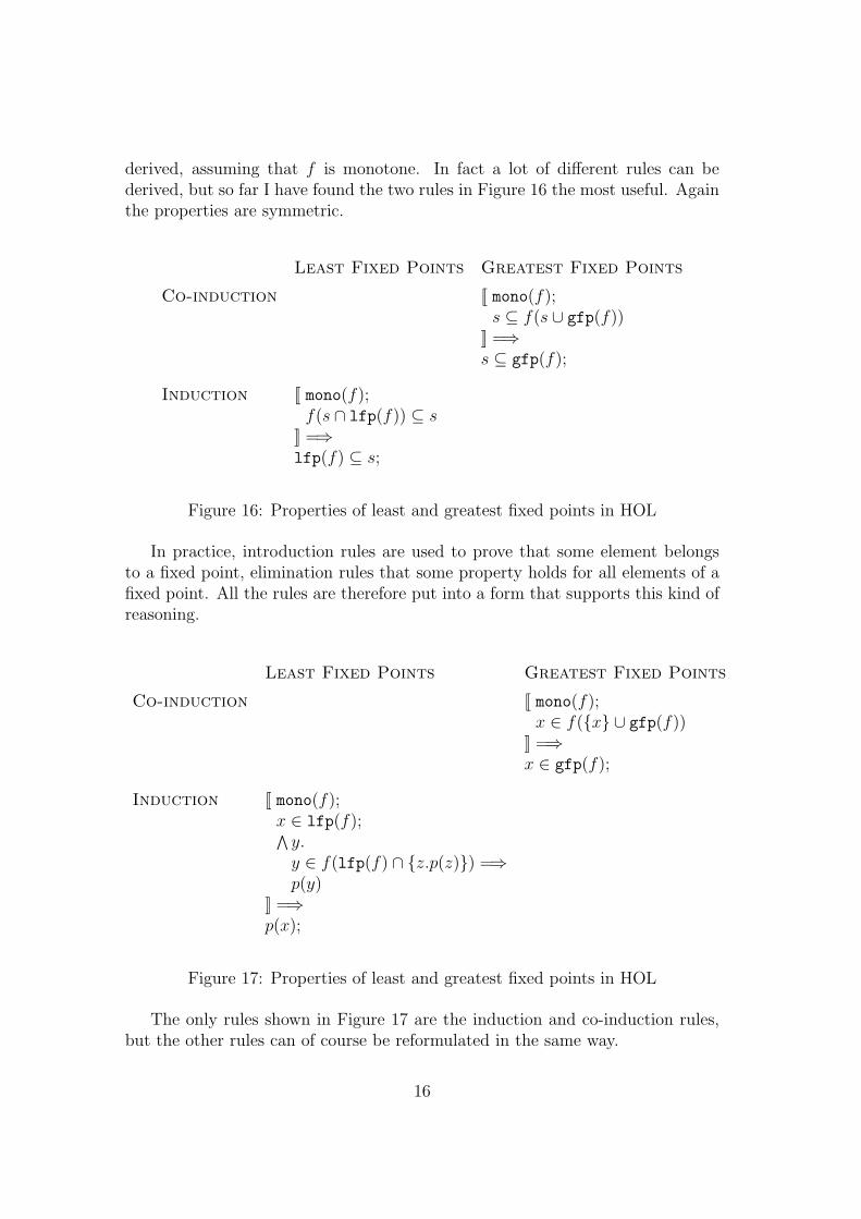
derived, assuming that f is monotone. In fact a lot of different rules can bederived, but so far I have found the two rules in Figure 16 the most useful. Againthe properties are symmetric.


Co-induction [[ mono(f);s ⊆ f(s ∪ gfp(f))

]] =⇒s ⊆ gfp(f);

Induction [[ mono(f);f(s ∩ lfp(f)) ⊆ s

]] =⇒lfp(f) ⊆ s;


In practice, introduction rules are used to prove that some element belongsto a fixed point, elimination rules that some property holds for all elements of afixed point. All the rules are therefore put into a form that supports this kind ofreasoning.


Co-induction [[ mono(f);x ∈ f({x} ∪ gfp(f))

]] =⇒x ∈ gfp(f);

Induction [[ mono(f);x ∈ lfp(f);∧y.y ∈ f(lfp(f) ∩ {z.p(z)}) =⇒p(y)

]] =⇒p(x);


The only rules shown in Figure 17 are the induction and co-induction rules,but the other rules can of course be reformulated in the same way.

16

Most of the rules described above come as part of a Isabelle HOL theory ofleast and greatest fixed points. It was however necessary to derive the form ofthe co-induction rule shown in Figure 16 and 17.

4.2 The Language

Expressions, defined by the BNF in Figure 1, can be formally expressed in Is-abelle HOL as a datatype. It can be done using the theory of least fixed points,but require quite a lot of tedious work. First the set of expressions must bedefined as the least fixed point of a suitable monotone function. Then, in orderto make expressions distinct from members of other types and to take advantageof Isabelle’s type system, the set of expressions should be related to an abstractmeta-level type of expressions. It can be done by declaring two isomorphismfunctions, an abstraction and a representation function. Using these, operationsand properties should be lifted to the abstract level. From then on, all reasoningshould take place at the abstract level. A description of the above method canbe found in [3].

The solution adapted here and in the following is to give an axiomatic spec-ification of datatypes. Of course there is a greater risk of introducing errors,but given the amount of work otherwise required, that the above method forformalising datatypes has been investigated elsewhere and that axiomatisation ofdatatypes is well understood, it seems a sensible choice.

A standard axiomatisation of expressions is shown in Figure 18. A type ofexpressions Ex is declared together with constants corresponding to the construc-tors of the datatype. There are rules stating that the constructors are distinctand injective. Because Ex is a datatype there is also an induction rule. Thereis no need for introduction rules, because the constructors have been declaredusing the typed lambda calculus. It also simplifies for example the inductionrule, because no type constraints have to appear explicitly.

Neither of the above solutions are very satisfactory. A much better solutionfrom a practical point of view is to use a (co)inductive package like that availablefor Isabelle HOL today. It will automatically provide the necessary properties,given the constructors and their types. Unfortunately this package was not avail-able at the time of formalisation.


Before the dynamic semantics can be formalised it is necessary to formalise thenotion of values, environments and closures. It might seem a relatively hard taskif it had to be done using greatest fixed points. Furthermore only a few obviousproperties are needed in order to prove consistency. All these properties holdfor every solution to the three equations (1)-(3) in Figure 2. The requirement(4) that the set of closures must contain all non-well-founded closures is not

17

Types

Const :: term ExVar :: term Ex :: term

Constants

e const :: Const⇒ Ex

e var :: ExVar⇒ Ex

(fn ⇒ ) :: [ExVar, Ex]⇒ Ex

(fix ( ) = ) :: [ExVar, ExVar, Ex]⇒ Ex

( @ ) :: [Ex, Ex]⇒ Ex

Injectiveness Axioms

e const(c1) = e const(c2) =⇒ c1 = c2;...

e11@e12 = e21@e22 =⇒ e11 = e21 ∧ e12 = e22;

Distinctness Axioms

e const(c) 6= e var(x); . . . e const(c) 6= e1@e2;...

fix f(x) = e1 6= e1@e2;

Induction Axiom

[[∧x.p(e var(x));∧c. p(e const(c));∧x e. p(e) =⇒ p(fn x⇒ e);∧f x e. p(e) =⇒ p(fix f(x) = e);∧e1 e2. p(e1) =⇒ p(e2) =⇒ p(e1@e2)

]] =⇒p(e);

Figure 18: Constants, variables and expressions in HOL

18

Types

Val :: term ValEnv :: term Clos :: term

Constantsv const :: Const⇒ Val

v clos :: Clos⇒ Val

ve emp :: ValEnv( + { 7→ }) :: [ValEnv, ExVar, Val]⇒ ValEnv

ve dom :: ValEnv⇒ ExVar set

ve app :: [ValEnv, ExVar]⇒ Val

(〈 , , 〉) :: [ExVar, Ex, ValEnv]⇒ Clos

c app :: [Const, Const]⇒ Const

Axioms

v const(c1) = v const(c2) =⇒ c1 = c2;v clos(〈x1, e1, ve1〉) = v clos(〈x2, e2, ve2〉) =⇒x1 = x2 ∧ e1 = e2 ∧ ve1 = ve2;v const(c) 6= v clos(cl);

ve dom(ve+ {x 7→ v}) = ve dom(ve) ∪ {x};ve app(ve+ {x 7→ v}, x) = v;x1 6= x2 =⇒ ve app(ve+ {x1 7→ v}, x2) = ve app(ve, x2);

Figure 19: Values, value environments and closures in HOL

directly relevant to the proof of consistency. In this light, it seems acceptablesimply to state the few obvious properties needed. These appear in Figure 19.It must however be considered a lacking feature of Isabelle HOL that there is noautomatic support for mutually recursive co-datatypes.

The inference system in Figure 3 can be seen as an inductive definition of arelation, in this case relating environments, expressions and values. Although thisis not stated explicitly, it is obviously a correct interpretation because consistencyis proved by induction on the depth of the inference in the original paper.

An inductive relation such as in Figure 3 can be represented as a set of triples.Here a triple consist of an environment, an expression and a value. Because therelation is defined inductively, the corresponding set can be defined as the leastfixed point of a function derived from the rules of the inference system. Theformalisation in Isabelle HOL is based on this idea and appear in Figure 20.

The function eval fun is obtained directly from the rules of the inferencesystem. For each rule all free variables are existentially quantified. The triple

19

Constants

eval fun :: (ValEnv ∗ Ex ∗ Val) set⇒ (ValEnv ∗ Ex ∗ Val) seteval rel :: (ValEnv ∗ Ex ∗ Val) set( ` =⇒ ) :: [ValEnv, Ex, Val]⇒ bool

Axioms

eval fun(s) ≡{ pp.

(∃ve c.pp = 〈〈ve, e const(c)〉, v const(c)〉)∨(∃ve x.pp = 〈〈ve, e var(x)〉, ve app(ve, x)〉 ∧ x ∈ ve dom(ve))∨(∃ve e x.pp = 〈〈ve, fn x⇒ e〉, v clos(〈x, e, ve〉)〉)∨( ∃ve e x f cl.pp = 〈〈ve, fix f(x) = e〉, v clos(cl∞)〉∧cl∞ = 〈x, e, ve+ {f 7→ v clos(cl∞)}〉

)∨( ∃ve e1 e2 c1 c2.pp = 〈〈ve, e1@e2〉, v const(c app(c1, c2))〉∧〈〈ve, e1〉, v const(c1)〉 ∈ s ∧ 〈〈ve, e2〉, v const(c2)〉 ∈ s

)∨( ∃ve ve′ e1 e2 e

′ x′ v v2.pp = 〈〈ve, e1@e2〉, v〉∧〈〈ve, e1〉, v clos(〈x′, e′, ve′〉)〉 ∈ s∧〈〈ve, e2〉, v2〉 ∈ s∧〈〈ve′ + x′ 7→ v2, e

′〉, v〉 ∈ s)};eval rel ≡ lfp(eval fun);ve ` e −→ v ≡ 〈〈ve, e〉, v〉 ∈ eval rel;

Figure 20: Evaluation in HOL

20

corresponding to the conclusion is claimed equal to pp. Every occurrence of therelation as a premise is translated to a corresponding triple and claimed to belongto the argument s of the function. Every other premise is translated directly intoa corresponding Isabelle HOL formula. Finally all the pieces are combined byconjunctions and disjunctions and packed into a set comprehension.

The formalisation of the dynamic semantics must be correct. Given the defi-nitions Figure 20, introduction rules very similar to the inference system can bederived. More importantly it is possible to derive an induction rule. Big induc-tion rules are notoriously difficult to write. The advantage of the approach usedhere, compared to an axiomatic approach is that it is possible to derive the cor-rect induction rule. Some of the introduction rules and the induction rule appearin Figure 21.

Although not very difficult, it is time consuming to define relations and deriveproperties as described above. Automating the process would save a lot of work.


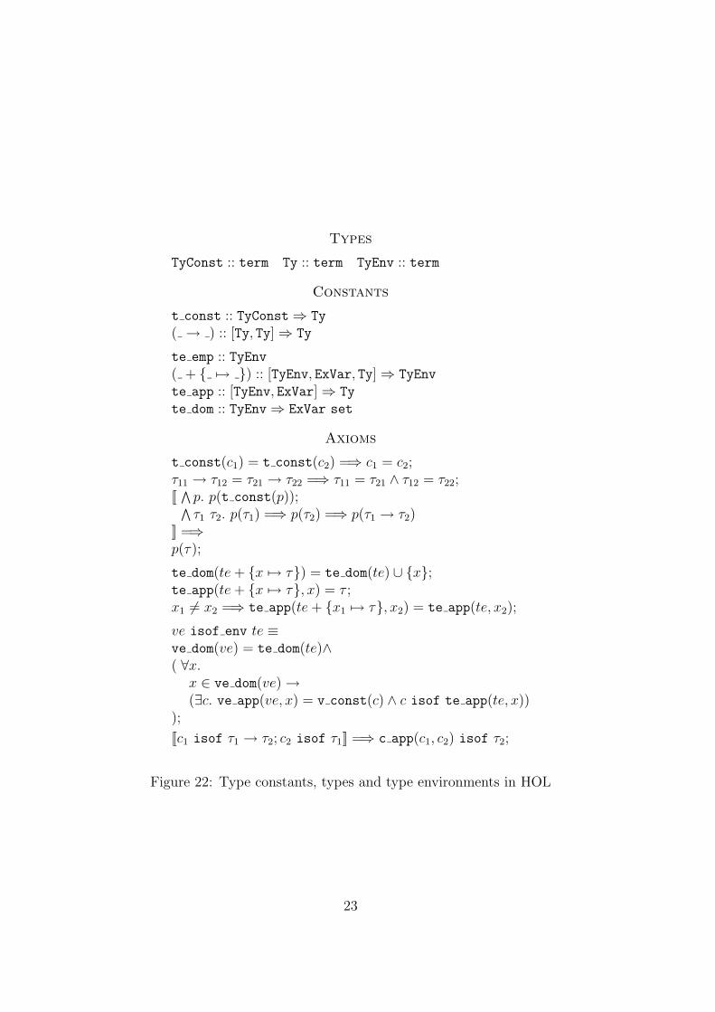
Before formalising the static semantics, it is necessary to formalise the notions oftypes, type environments etc. This is done in Figure 22 and Figure 23.

The type of types is another example of a construct that could be formalisedas a datatype using the theory of least fixed points. But as before, and for thesame reasons, this is not done. Instead it is specified axiomatically. In fact onlythe properties needed for this paper are stated. Similar for the notion of typeenvironments.

Just as it was the case in the original paper, the existence of a correspondencerelation, relating constants to their type is claimed. The requirement that thisshould be consistent with application of constants is taken directly from theoriginal paper.

The actual inference system can again be seen as an inductive definition of arelation. Again, it is formalised in Isabelle HOL, using the theory of least fixedpoints. The formalisation appears in Figure 24.

Surprisingly, the fact that the relation is defined as the least fixed point andtherefore enjoys an induction rule is never used in the proof of consistency. Itis only necessary to use ordinary elimination and it would have been possible touse the greatest fixed point for the definition instead.

The inference system has an interesting and very useful property. In a deriva-tion of a statement ve ` e =⇒ τ , only one rule can have been used for the lastinference. The reason is that there is exactly one rule for each kind of expression.As a consequence, knowing that ve ` e =⇒ τ hold it possible to conclude that thepremises of the corresponding rule hold. In other words it is possible to use eachof the rules backward. This kind of reasoning is used in the proof of consistency.The ordinary elimination rule and derived elimination rules allowing the kind ofreasoning just described, are shown in Figure 25.

21

Introduction

ve ` e const(c) −→ v const(c);x ∈ ve dom(ve) =⇒ e ` e var(x) −→ ve app(ve, x);

...[[ ve ` e1 −→ v clos(〈x′, e′, ve′〉);ve ` e2 −→ v2;ve′ + {x′ 7→ v2} ` e′ −→ v

]] =⇒ve ` e1@e2 −→ v;

Induction

[[ ve ` e −→ v;∧ve c. p(ve, e const(c), v const(c));∧x ve. x ∈ ve dom(ve) −→ p(ve, e var(x), ve app(ve, x));∧x ve e. p(ve, fn x⇒ e, v clos(〈x, e, ve〉));∧x f ve cl∞ e.cl∞ = 〈x, e, ve+ {f 7→ v clos(cl∞)}〉 =⇒p(ve, fix f(x) = e, v clos(cl∞));∧ve c1 c2 e1 e2.[[ p(ve, e1, v const(c1)); p(ve, e2, v const(c2)) ]] =⇒p(ve, e1@e2, v const(c app(c1, c2)));∧ve ve′ x′ e1 e2 e

′ v v2.[[ p(ve, e1, v clos(〈x′, e′, ve′〉));p(ve, e2〉, v2〉);p(ve′ + {x′ 7→ v2}, e′, v)

]] =⇒p(ve, e1@e2, v)

]] =⇒p(ve, e, v);

Figure 21: Properties of evaluation in HOL

22

Types

TyConst :: term Ty :: term TyEnv :: term

Constants

t const :: TyConst⇒ Ty

( → ) :: [Ty, Ty]⇒ Ty

te emp :: TyEnv( + { 7→ }) :: [TyEnv, ExVar, Ty]⇒ TyEnv

te app :: [TyEnv, ExVar]⇒ Ty

te dom :: TyEnv⇒ ExVar set

Axioms

t const(c1) = t const(c2) =⇒ c1 = c2;τ11 → τ12 = τ21 → τ22 =⇒ τ11 = τ21 ∧ τ12 = τ22;[[∧p. p(t const(p));∧τ1 τ2. p(τ1) =⇒ p(τ2) =⇒ p(τ1 → τ2)

]] =⇒p(τ);

te dom(te+ {x 7→ τ}) = te dom(te) ∪ {x};te app(te+ {x 7→ τ}, x) = τ ;x1 6= x2 =⇒ te app(te+ {x1 7→ τ}, x2) = te app(te, x2);

ve isof env te ≡ve dom(ve) = te dom(te)∧( ∀x.x ∈ ve dom(ve)→(∃c. ve app(ve, x) = v const(c) ∧ c isof te app(te, x))

);

[[c1 isof τ1 → τ2; c2 isof τ1]] =⇒ c app(c1, c2) isof τ2;

Figure 22: Type constants, types and type environments in HOL

23

Constants

( isof ) :: [Const, Ty]⇒ bool

( isof env ) :: [ValEnv, TyEnv]⇒ bool

Axioms

ve isof env te ≡ve dom(ve) = te dom(te)∧( ∀x.x ∈ ve dom(ve)→(∃c. ve app(ve, x) = v const(c) ∧ c isof te app(te, x))

);

[[c1 isof τ1 → τ2; c2 isof τ1]] =⇒ c app(c1, c2) isof τ2;

Figure 23: Basic correspondence relation in HOL

To derive the last rules it is of course necessary to use properties of expressions.They are proved in a few lines by invoking a classical reasoning tactic with aproper set of rules. Similar for the rest of the rules, it cannot be claimed thatthey are difficult to derive. It is, however, very time consuming.

4.5 Consistency

The formalisation of consistency is divided into two parts. First it is consideredhow to state consistency in Isabelle HOL, then how to prove it.

4.5.1 Stating Consistency

Stating consistency proceeds just as in the original paper. The real interest is onproving basic consistency. In order to do that, is necessary to state and provethe stronger consistency result. This result is stated using an extended versionof the correspondence relation isof.

The effort is concentrated on defining the extended correspondence relationand proving some properties about it. In the original paper it is defined as thegreatest fixed point of a function. The formal definition is very similar. The onlyreal difference is the style used to write the function. Here the style used is thesame as was used to formalise the inference systems. In other words the newcorrespondence relation is a co-inductive relation defined by two rules. Makingthe formalisation consistent with the previous formalisations of inference systems,allows one to prove properties in a uniform way. It is for example easy to prove thefunction monotone using the same tactic as earlier. Worries that errors mighthave been introduced in the reformulation is not important as long as basic

24

Constants

elab fun :: (TyEnv ∗ Ex ∗ Ty) set⇒ (TyEnv ∗ Ex ∗ Ty) setelab rel :: (TyEnv ∗ Ex ∗ Ty) set( ` =⇒ ) :: [TyEnv, Ex, Ty]⇒ bool

Axioms

elab fun(s) ≡{ pp.

(∃te c τ.pp = 〈〈te, e const(c)〉, t〉 ∧ c isof τ)∨(∃te x.pp = 〈〈te, e var(x)〉, te app(te, x)〉 ∧ x ∈ te dom(te))∨(∃te x e τ1 τ2.pp = 〈〈te, fn x⇒ e〉, τ1 → τ2〉 ∧ 〈〈te+ {x 7→ τ1}, e〉, τ2〉 ∈ s)∨( ∃te f x e τ1 τ2.pp = 〈〈te, fix f(x) = e〉, τ1 → τ2〉∧〈〈te+ {f 7→ τ1 → τ2}+ {x 7→ τ1}, e〉, τ2〉 ∈ s

)∨( ∃te e1 e2 τ1 τ2 .pp = 〈〈te, e1@e2〉, τ2〉 ∧ 〈〈te, e1〉, τ1 → τ2〉 ∈ s ∧ 〈〈te, e2〉, τ1〉 ∈ s

)};elab rel ≡ lfp(elab fun);te ` e =⇒ τ ≡ 〈〈te, e〉, τ〉 ∈ elab rel;

Figure 24: Elaboration in HOL

consistency can be proved. The only purpose of the extended correspondencerelation and consistency is to prove basic consistency. Basic consistency doesnot refer to the extended correspondence relation and does therefore not dependon the formulation of this relation. The Isabelle HOL formalisation is shown inFigure 26.

From these definitions it is straightforward to derive introduction rules andelimination rules as it has been done earlier. More interestingly it is possible toderive the co-induction rules shown in Figure 27.

Because co-induction is introduction there are of course two co-induction rules.These are based on the strong form of co-induction shown in Figure 17. It isdifferent from the form of co-induction used in [2], which is the weak form shownearlier. It turns out that the use of the strong form of co-induction shortens theproof, further backing the claim that this is a useful formulation of co-induction.

Formalising the new correspondence relation is similar to formalising the in-ference systems and just as time consuming. The conclusion is of course thatIsabelle should have automatic support for co-inductive definitions, as provided

25

Ordinary Elimination

[[ te ` e =⇒ τ ;∧te c τ. c isof t =⇒ p(te, e const(c), τ);∧te x. x ∈ te dom(te) =⇒ p(te, e var(x), te app(te, x));∧te x e τ1 τ2. te+ {x 7→ τ1} ` e =⇒ τ2 =⇒ p(te, fn x⇒ e, τ1 → τ2);∧te f x e τ1 τ2.te+ {f 7→ τ1 → τ2}+ {x 7→ τ1} ` e =⇒ τ2 =⇒ p(te, fix f(x) = e, τ1 → τ2);∧te e1 e2 τ1 τ2.[[te ` e1 =⇒ τ1 → τ2; te ` e2 =⇒ τ1]] =⇒ p(te, e1@e2, τ2)

]] =⇒p(te, e, t);

Elimination for Each Expression

te ` e const(c) =⇒ τ =⇒ c isof τ ;te ` e var(x) =⇒ τ =⇒ τ = te app(te, x) ∧ x ∈ te dom(te);

...te ` e1@e2 =⇒ τ2 =⇒ (∃τ1. te ` e1 =⇒ τ1 → τ2 ∧ te ` e2 =⇒ τ1);

Figure 25: Properties of elaboration in HOL

by the (co)inductive package which now exists.Now it is possible to state consistency in Isabelle HOL. The formulation of

consistency given here differs from the original. The reason is that the formulationof consistency in the original is not suitable for doing a formal proof. For theproof to proceed smoothly it is necessary to reformulate it slightly as in Figure28. Basic consistency in Figure 28 is translated directly from the original paper.

4.5.2 Proving Consistency

It turned out to be surprisingly easy to prove the consistency result. The proofproceeds more or less as the original proof.

The first step in the original proof was to use induction on the depth of theinference of evaluations. Here consistency is proved by induction on the structureof evaluations which is basically the same.

It is in connection with the application of induction that the only real difficultyof formalising the proof occur. Exactly what should the induction rule be appliedto ? This is not obvious because the induction rule can be applied to almostanything.

The original formulation of consistency suggests to use the induction ruleon te ` e =⇒ τ → v hasty τ . Attempting to prove consistency this way

26

Constants

hasty fun :: (Val ∗ Ty) set⇒ (Val ∗ Ty) sethasty rel :: ”(Val ∗ Ty) set( hasty ) :: [Val, Ty]⇒ bool

( hasty env ) :: [ValEnv, TyEnv]⇒ bool

Axioms

hasty fun(s) ≡{ p.

(∃c τ. p = 〈v const(c), τ〉 ∧ c isof τ)∨( ∃x e ve τ te.p = 〈v clos(〈x, e, ve〉), τ〉∧te ` fn x⇒ e =⇒ τ∧ve dom(ve) = te dom(te)∧(∀x1.x1 ∈ ve dom(ve)⇒ 〈ve app(ve, x1), te app(te, x1)〉 ∈ s)

)};hasty rel ≡ gfp(hasty fun);v hasty τ ≡ 〈v, τ〉 ∈ hasty rel;ve hasty env te ≡ve dom(ve) = te dom(te)∧(∀x. x ∈ ve dom(ve)⇒ ve app(ve, x) hasty te app(te, x));

Figure 26: Extended correspondence relation in HOL

fails, because the induction hypothesises are too weak. This is the reason whyconsistency has been reformulated here. Besides rearranging the premises, τ andte have been explicitly quantified. Using the new formulation, consistency isproved by using the induction rule on ∀τ te. ve hasty env te→ te ` e =⇒ τ →v hasty τ .

The above should not be seen as a problem of formalisation, but rather as aproblem of proof. The original paper should state exactly what formula inductionshould be applied to.

Having applied induction six cases remain to be proved, one for each of therules of the dynamic semantics.

The first two cases, the ones for constants and variables, are claimed to betrivial in the original paper. Here they both have three lines proofs, of which onlytwo lines are interesting. Both are proved by first using one of the eliminationrules for elaborations and then an introduction rule for the extended correspon-dence relation or a call of a classical reasoning tactic.

27

c isof τ =⇒ 〈v const(c), τ〉 ∈ hasty rel;

[[ te ` fn x⇒ e =⇒ τ ;ve dom(ve) = te dom(te);∀x1.x1 ∈ ve dom(ve)→〈ve app(ve, x1), te app(te, x1)〉 ∈ {〈v clos(〈x, e, ve〉), τ〉} ∪ hasty rel

]] =⇒〈v clos(〈x, e, ve〉), τ〉 ∈ hasty rel;

Figure 27: Co-induction rules for hasty rel in HOL

Consistency

ve ` e −→ v =⇒ (∀τ te. ve hasty env te→ te ` e =⇒ τ −→ v hasty τ);

Basic Consistency

[[ve isof env te; ve ` e −→ v const(c); te ` e =⇒ τ ]] =⇒ c isof τ ;

Figure 28: Consistency in HOL

In the original paper, they spend a little space on the third case, the onefor abstraction. Here it seems just as trivial to prove as the first two. First anintroduction rule for the extended correspondence relation is used, then a classicalreasoning tactic.

The fourth case, the one for recursive functions, is the most interesting inthat it uses co-induction. In the paper the proof takes up a little more thanhalf a page. The formal proof is about 25 lines. The proof uses elimination onelaborations, some set theoretic reasoning, classical reasoning tactics etc. andof course co-induction. The stronger co-induction rule used here simplifies theproof, backing the claim that it is a useful formulation of co-induction.

The fifth case, the one for application of constants, is one of those claimedto be trivial in the original paper. Here it is however more complicated than thefirst three cases. It uses elimination on both elaborations and on the extendedcorrespondence relation, as well as several calls of classical reasoning tactics. Italso uses the requirement that the relation isof must be consistent with thefunction apply. Still the proof consists of less than 10 lines.

The last case, the one for application of closures, is the case that takes upmost space in the original paper. Here it is shorter than the one for recursivefunctions. The proof uses elimination on elaborations and on hasty, classicalreasoning tactics etc.

28

With the original proof guiding the formal proof, it was straightforward tocarry out in Isabelle HOL. Filling in the necessary details required surprisinglylittle knowledge of how consistency actually was proved. It was a very positiveexperience.

4.6 Discussion

4.6.1 Inductive and Co-inductive Definitions

The case study considered here illustrates in no uncertain manner how useful,especially inductive, but also co-inductive definitions are in computer science.

An estimated 4/5 of the work presented here is related to the formalisation ofinductive and co-inductive definitions of relations and datatypes. In the case ofrelations, the Isabelle theory of least and greatest fixed points were used, whilethe datatypes were specified axiomatically. Even more work would have beenrequired, if the formalisation of datatypes, had been based on the fixed pointtheory of Isabelle.

The above clearly shows the need for a (co)inductive package for Isabelle HOL.From a practical point of view, it is of course highly unsatisfactory that the bulkof work is concentrated on tedious and time consuming tasks, that could just aswell be done automatically.

A (co)inductive package should not only provide the obvious abstract proper-ties for (co)inductive definitions. It should also support reasoning about (co)in-ductively defined objects. Consider for example the present case study. It wouldhave been useful if special elimination rules like those in Figure 25 had beenderived automatically. It would also be useful if the package supported simpleclassical reasoning about the (co)inductively defined constructs.

Although not available at the time of formalisation, a (co)inductive packagefor Isabelle HOL now exists [10]. It is derived from the corresponding packagefor Isabelle ZF, but does not support co-datatypes. Using this package it shouldbe possible to improve the formalisation described above considerably.

4.6.2 Avoiding Co-induction

Although not really the subject here, it could be argued that there is no need forusing co-induction to prove consistency.

It seems to be perfectly possible to do the consistency proof without using co-induction. One could work with a finite representation of the non-well-foundedclosures. At first the notion of co-inductive definitions and proofs might be over-whelming and this solution therefore seem compelling. Co-inductive definitionsand proofs are however, perfectly natural and mechanically tractable notions. Itherefore see no practical justification for using finite representations, if the pos-sibility of using the more abstract notions of co-inductive definitions and proofs

29

are present.

4.6.3 Working with Isabelle HOL

Disregarding the lack of inductive and co-inductive definitions, at the time offormalisation, working with Isabelle HOL was a positive experience.

As already mentioned, doing the actual proof of consistency turned out to besurprisingly easy. The original proof could be used as an outline. From thereon it was just a question of filling in a few details, a task which hardly requiredany knowledge of what was going on. Difficulties were only encountered whenthe original proof was not as clear as one could have wished, for example withrespect to exactly what induction should be applied to. This must however beconsidered a problem of proof, not formalisation. Another remarkable fact isthat the formal proof only takes up about the same space as the original proof.This contradicts, what seems to be the common conception, that formal proofsnecessarily are long and much harder to do than corresponding informal proofs.

A nice feature of Isabelle is its tactics and tacticals. The classical reasoningtactics proved especially useful. The possibility of defining new tactics was onlyreally exploited once, to write a tactic for proving functions corresponding to in-ference systems monotone. Writing good tactics is a difficult and time consumingjob and instead of writing new tactics, one tends to use tactics already available.Their real potential seems to be when developing new theories which are intendedto be used by others. Such theories should come with tactics for reasoning in thenew theory.

5 Formalisation in Isabelle ZF

At first sight it might seem a vain undertaking to carry of the same formaldevelopment in ZF as has already been carried out in HOL. There are however anumber of reasons for doing it.

ZF and HOL are different logics. The development in ZF provide an oppor-tunity to study some of the consequences of these differences, in particular theconsequences with regard to non-well-founded objects.

The formalisation of the consistency result in ZF turned out to be one real-istic (co)inductive definition after another. In other words it is a good examplefor testing the (co)inductive package in ZF. Testing should be understood in abroader sense, covering not only the practical aspect of testing for bugs, but alsothe actual design of the package.

The formal development in HOL was carried out without the use of a (co)in-ductive package. It was claimed that a (co)inductive package would be a hugeimprovement and estimates of the resulting reductions in workload was given. A

30

similar development in ZF make it possible to verify the claim and substantiatethe estimates further, or possibly reject the claim.

The structure of this section follows that of §2 and §4.

5.1 The Language

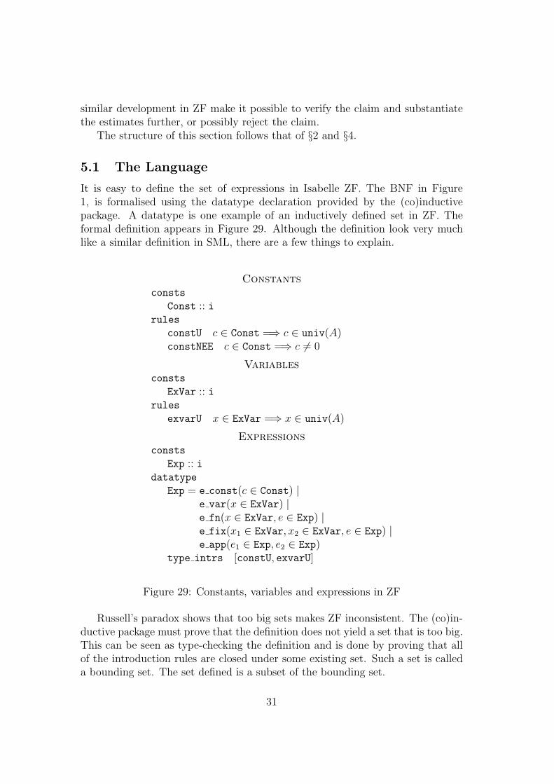
It is easy to define the set of expressions in Isabelle ZF. The BNF in Figure1, is formalised using the datatype declaration provided by the (co)inductivepackage. A datatype is one example of an inductively defined set in ZF. Theformal definition appears in Figure 29. Although the definition look very muchlike a similar definition in SML, there are a few things to explain.

Constantsconsts

Const :: irules

constU c ∈ Const =⇒ c ∈ univ(A)constNEE c ∈ Const =⇒ c 6= 0

Variablesconsts

ExVar :: irules

exvarU x ∈ ExVar =⇒ x ∈ univ(A)

Expressionsconsts

Exp :: idatatype

Exp = e const(c ∈ Const) |e var(x ∈ ExVar) |e fn(x ∈ ExVar, e ∈ Exp) |e fix(x1 ∈ ExVar, x2 ∈ ExVar, e ∈ Exp) |e app(e1 ∈ Exp, e2 ∈ Exp)

type intrs [constU, exvarU]

Figure 29: Constants, variables and expressions in ZF

Russell’s paradox shows that too big sets makes ZF inconsistent. The (co)in-ductive package must prove that the definition does not yield a set that is too big.This can be seen as type-checking the definition and is done by proving that allof the introduction rules are closed under some existing set. Such a set is calleda bounding set. The set defined is a subset of the bounding set.

31

The standard bounding set for a datatype definition with parametersA1, . . . , An is univ(A1 ∪ . . . ∪An). This set contains A1 ∪ . . . ∪An, and is closedunder paring, left and right injections; the constructs used to define the datatype.The bounding set for the definition of Exp is univ(0) because the definition hasno parameters. To type-check the definition of Exp, all of the rules must be closedunder univ(0). For example, to prove that the rule for function abstraction isclosed, the package must prove:

[[x ∈ ExVar; e ∈ univ(0)]] =⇒ e fn(x, e) ∈ univ(0)

The extra rules needed by the package to type-check a definition is given in thetype intrs . . . part of the definition. In order to type-check the definition of Exp,the unspecified sets ExVar and Const must both be subsets of the bounding setuniv(0). This explains the role of the two axioms constU and exvarU in Figure29. The presence of the axiom constNEE is explained in §5.2.2.

Given the definition in Figure 29 the package defines the set Exp and allthe constructors. It will also derive the usual rules: introduction, elimination,induction, injectiveness and distinctness. It does however not relate the definedset to an abstract set by two isomorphism functions, as discussed in section 4.2.As a consequence, elements of different datatypes may be identical.

An alternative approach is to parametrise the definition of Exp by two setscorresponding to Const and ExVar. They would then automatically be includedin the bounding set. It is difficult to say which solution is the best, as the lattermethod would require other sets depending on Exp to be parametrised as well.

The amount of work done by the package is substantial. Because all datatypeswas axiomatised in HOL, it is not possible to do a direct comparison. It ishowever clear that the package is a huge improvement; the reason for axiomatisingdatatypes in HOL was the amount of work required if they where to be defined byhand. Now the definition in ZF takes up noticeable less space than the axiomaticspecification given in HOL and are closer to the original specification.


Before the notion of values are formalised, a notion of variant maps are defined.After that the section follows the usual pattern.

5.2.1 Variant Maps

Sets in ZF must be well-founded by the foundation axiom:

A = 0 ∨ (∃x ∈ A.∀y ∈ x.y /∈ A)

The foundation axiom outlaws infinite descents under the membership relation.Take, for example an equation like a = {a}. Any solution to this must be non-

32

well-founded, but it can clearly not have any solution in ZF as it would lead toan infinite decent:

. . . ∈ {. . .} ∈ {{. . .}}

Another example is infinite lists encoded using the standard notion of pair in ZF:

〈a, b〉 ≡ {{a}, {a, b}}

The infinite list with elements a1, a2 . . . would be:

〈a1, 〈a2, . . .〉〉 = {{a1}, {a1, {{a2}, {a2, . . .}}}}

Such an infinite list cannot be a set in ZF because there exists an infinite decent:

. . . ∈ {a2, . . .} ∈ 〈a2, . . .〉 ∈ {a1, 〈a2, . . .〉} ∈ 〈a1, 〈a2, . . .〉〉

The above might give the impression that co-datatypes are of very limited usein ZF. If encoded using ordinary pairs the set of lazy lists would for example beexactly the same as the set of finite lists. Fortunately it is possible to circumventthe problem by defining a new notion of pairs; the variant pair [6].

Keeping in mind, that everything is a set in ZF, the variant notion of pair isdefined as:

〈a; b〉 ≡ ({0} × a) ∪ ({1} × b) = a+ b

Using the new notion of pair to encode lists, the infinite list with elementsa1 = {a11, . . . , a1m}, a2 = {a21, . . . , a2n}, . . . is:

〈a1; 〈a2; . . .〉〉 = {〈0, a11〉, . . . 〈0, a1m〉, 〈1, 〈0, a21〉〉, . . . 〈1, 〈0, a2n〉〉, . . .}

As it appears there are no infinite descents, when using the variant representationof pair, although the list is infinite.

When doing (co)inductive definitions such as co-datatype definitions, it iscrucial to use the right representations to avoid forcing sets to be well-founded.The (co)inductive package is therefore based on a theory of variant pairs, anduses them when necessary [7]. This does however not free the user of the packagefrom being cautious.

In the next section value environments are going to be represented as whatis basically functions. The standard representation of functions in ZF is as setsof pairs. Value environments will be defined as a part of a mutual co-datatypedefinition. Using the standard function space in ZF to represent value environ-ments, would lead to a problem similar to the problem of infinite lists above. Toovercome this problem the notion of variant maps (functions) is introduced.

A variant map is a generalisation of a variant pair. A variant pair is a sum(a+b) and a variant map is a general sum (Σx∈a.bx) [6]. The set of all variantmaps can easily be defined directly from the set of standard maps by converting

33

each standard map into a variant map. Unfortunately such a definition makesreasoning hard. An alternative approach, where a slightly too big set is restrictedto the desired set, has therefore been adopted instead. The formal definition of theset TMap(A,B) of total maps from A to B and the set of partial maps Map(A,B)from A to B, as well as some of the associated operations can be found in Figure30.

consts

TMap :: [i, i]⇒ i

Map :: [i, i]⇒ i

rules

TMap def TMap(A,B) ≡ {m ∈ Pow(A× ⋃B).∀a ∈ A.m“{a} ∈ B}Map def Map(A,B) ≡ TMap(A, cons(0, B))

consts

map emp :: imap owr :: [i, i, i]⇒ i

map app :: [i, i]⇒ i

rules

map emp def map emp ≡ 0map owr def map owr(m, a, b) ≡ Σx∈{a}∪domain(m)if(x = a, b,m“{x})map app def map app(m, a) ≡ m“{a}

Figure 30: Variant maps in ZF

The set Pow(A × ⋃B) is too big to be TMap(A,B) because an element of Acould be mapped to a mix of elements from B. It is easy to see that this mixdo not necessarily belong to B itself. If for example B is the set {{b1}, {b2}},an element of A might be mapped to {b1, b2}, which clearly is not a member ofB. The predicate ∀a ∈ A.m“{a} ∈ B therefore requires that all elements in A ismapped to an element in B. To see this, simply view a map as a relation on Aand

⋃B. Application then becomes the image of a singleton set.

It is interesting to see what happens to TMap(A,B) if B contains the empty set0. In this case total maps effectively becomes partial maps, as it is impossible totell whether an element of A is not in the domain of the map or just mapped to 0.This fact is exploited in defining the set of partial maps. The set of partial maps isthe corresponding set of total maps, with the empty set added to the range. It iseasy to define the usual operations on maps: domain, overwriting and application.All the definitions, except for the definition of domain appear in Figure 30. Thedomain of a map is simply the domain (domain) of the corresponding relation.

Proving the necessary properties about variant maps required some effort.This is not very surprising as the theory of variant maps is new. With a well

34

developed theory of variant notions, only a little effort would have been required.The properties proved is similar to those one would expect for maps based

on the ordinary notion of pairs. The main difference is that it is necessary to becareful about empty sets as elements. An example is the following theorem:

b 6= 0 =⇒ domain(map owr(m, a, b)) = {a} ∪ domain(m)

Here it is necessary to ensure that b is not the empty set, because if this wherethe case, the modification of m would have no effect.

5.2.2 Values and Value Environments

Closures can be non-well-founded. As a consequence, a co-datatype declarationis used to formalise the notion of values, value environments and closures. Us-ing a datatype declaration would only allow well-founded closures. The formaldefinition appear in Figure 31.

In order to simplify matters, no separate set for closures is defined. The set ofclosures has been eliminated by substituting the right hand side of (3) for Clos in(1). The two remaining sets Val and ValEnv are defined as a mutual co-datatype.The default name for the combined set of values and value environments definedby the package is Val ValEnv.

There are two constructors for values, one for constants and one for closures.A value environment is basically a variant map and consequently only one con-structor exists. As mentioned in the previous section, it is not possible to usethe ordinary function space to formalise the notion of value environments, as thiswould force all closures to be well-founded.

The default bounding set for a co-datatype with parameters A1, . . . , An isquniv(A1∪ . . .∪An), a superset of univ(A1∪ . . .∪An), which is also closed underthe variant constructions used by the package in (co)datatype definitions. Therules in the type intrs . . . part of the definition enable the package to prove thatthe rules are closed under quniv(0). The rule for variant maps mapQU is howevernot as one might expect:

[[m ∈ PMap(A, quniv(B));∧x.x ∈ A =⇒ x ∈ univ(B)]] =⇒ m ∈ quniv(B)

In this case it requires ExVar to be a subset of univ(0) instead of quniv(0). Itis therefore also necessary to include exvarU in the list of rules supplied to thepackage.

The operations on value environments are defined in terms of the case analysisoperator provided by the package and the operators on maps. A separate caseanalysis operator for each of the mutually defined sets would make the definitionssmaller and more readable.

The necessary properties about values and value environments are provedusing properties of maps and the rules derived by the package. The (co)inductive

35

consts

Val :: i ValEnv :: i Val ValEnv :: icodatatype

Val = v const(c ∈ Const) |v clos(x ∈ ExVar, e ∈ Exp, ve ∈ ValEnv) and

ValEnv = ve mk(m ∈ Map(ExVar, Val))monos [map mono]type intrs [constQU, exvarQU, exvarU, expQU, mapQU]

consts

ve emp :: ive owr :: [i, i, i]⇒ i

ve dom :: i⇒ i

ve app :: [i, i]⇒ i

rules

ve emp def

ve emp ≡ ve mk(map emp)ve owr def

ve owr(ve, x, v) ≡ve mk(Val ValEnv case(λx.0, λx y z.0, λm.map owr(m,x, v), ve))

ve dom def

ve dom(ve) ≡ Val ValEnv case(λx.0, λx y z.0, λm.domain(m), ve)ve app def

ve app(ve, a) ≡Val ValEnv case(λx.0, λxyz.0, λm.map app(m, a), ve)

Figure 31: Values and value environments in ZF

36

package automatically proves most of the properties needed, but it would havebeen useful if the function mk cases could have been used to derive specialisedelimination rules for each of the two sets Val and ValEnv. The problem of havingempty sets in the range of maps shows up here again. In order to prove consistencylater it is necessary to prove that no value is the empty set. A consequence isthat the set of constants must not contain the empty set as an element. Thisexplain the role of the axiom constNEE in Figure 29.

Because the notion of values, value environments and closure was axiomatisedin HOL it is again difficult to do a direct comparison. It is however clear thatmuch more work would have been required in HOL, if the formalisation wasdone in the same way as in ZF, but without a (co)inductive package. If theformalisation was carried in HOL using the (co)inductive package, ZF would havea small handicap, because of the way it treats non-well-founded constructions andbecause type-constraints must be handled explicitly.

As an alternative to using variant maps, value environments could be lazylists. Although the definition of the set of values and the set of value environmentswould be easier, it would be harder to define the operations on maps, and maybealso to reason about those. I cannot say which solution is the best.

5.2.3 Evaluation

The original inference system constitutes an inductive definition of a evaluationrelation between environments, expressions and values; a set of triples. It is easilyformalised in ZF as an inductive definition using the (co)inductive package. Allit takes is changing the syntax and adding a few things such as type constraintsand the rules needed for showing that the rules are closed under the boundingset.

In Figure 32, the domains . . . part of the definition state the name of therelation (EvalRel) and the bounding set (ValEnv× Exp× Val). The set definedmust be a subset of the bounding set. The rules given in the type intrs . . . partallow the package to prove that the rules are closed under the bounding set. Incontrast to (co)datatypes these rules are no longer concerned with univ(. . .) andquniv(. . .), because the bounding set is no longer one of these.

The size of the definitions in HOL and ZF are similar. However, much lessneeds to be proved in ZF. The proofs needed to derive the necessary rules wasaround 125 lines in HOL, while none where needed in ZF.


The (co)inductive package makes it very easy to formalise the static semantics.Before the notion of elaboration is formalised a notion of type, type environmentsand correspondence of constants and types are formalised.

37

consts

EvalRel :: iinductive

domains EvalRel ⊆ ValEnv× Exp× Val

intrs

eval constI

[[ve ∈ ValEnv; c ∈ Const]] =⇒〈ve, e const(c), v const(c)〉 ∈ EvalRel

eval varI

[[ve ∈ ValEnv;x ∈ ExVar;x ∈ ve dom(ve)]] =⇒〈ve, e var(x), ve app(ve, x)〉 ∈ EvalRel

eval fnI

[[ve ∈ ValEnv;x ∈ ExVar; e ∈ Exp]] =⇒〈ve, e fn(x, e), v clos(x, e, ve)〉 ∈ EvalRel

eval fixI

[[ve ∈ ValEnv;x ∈ ExVar; e ∈ Exp; f ∈ ExVar; cl ∈ Val;v clos(x, e, ve owr(ve, f, cl)) = cl

]] =⇒〈ve, e fix(f, x, e), cl〉 ∈ EvalRel

eval appI1

[[ve ∈ ValEnv; e1 ∈ Exp; e2 ∈ Exp; c1 ∈ Const; c2 ∈ Const;〈ve, e1, v const(c1)〉 ∈ EvalRel;〈ve, e2, v const(c2)〉 ∈ EvalRel

]] =⇒〈ve, e app(e1, e2), v const(c app(c1, c2))〉 ∈ EvalRel

eval appI2

[[ve ∈ ValEnv; ve′ ∈ ValEnv; e1 ∈ Exp;e2 ∈ Exp; e′ ∈ Exp;x′ ∈ ExVar; v ∈ Val;〈ve, e1, v clos(x′, e′, ve′)〉 ∈ EvalRel;〈ve, e2, v2〉 ∈ EvalRel;〈ve owr(ve′, x′, v2), e′, v〉 ∈ EvalRel

]] =⇒〈ve, e app(e1, e2), v〉 ∈ EvalRel

type intrs

c appI :: ve appI :: ve empI :: ve owrI ::Exp.intrs@Val ValEnv.intrs

Figure 32: Evaluation in ZF

38

5.3.1 Types and Type Environments

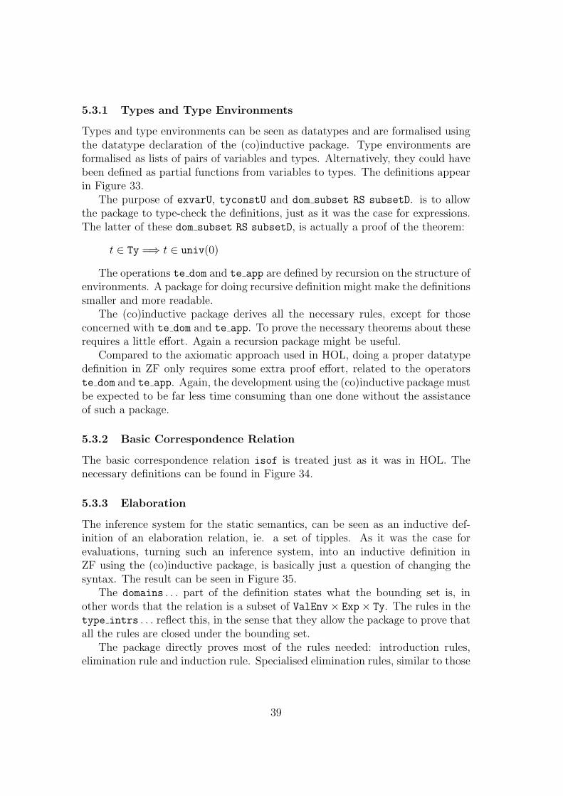
Types and type environments can be seen as datatypes and are formalised usingthe datatype declaration of the (co)inductive package. Type environments areformalised as lists of pairs of variables and types. Alternatively, they could havebeen defined as partial functions from variables to types. The definitions appearin Figure 33.

The purpose of exvarU, tyconstU and dom subset RS subsetD. is to allowthe package to type-check the definitions, just as it was the case for expressions.The latter of these dom subset RS subsetD, is actually a proof of the theorem:

t ∈ Ty =⇒ t ∈ univ(0)

The operations te dom and te app are defined by recursion on the structure ofenvironments. A package for doing recursive definition might make the definitionssmaller and more readable.

The (co)inductive package derives all the necessary rules, except for thoseconcerned with te dom and te app. To prove the necessary theorems about theserequires a little effort. Again a recursion package might be useful.

Compared to the axiomatic approach used in HOL, doing a proper datatypedefinition in ZF only requires some extra proof effort, related to the operatorste dom and te app. Again, the development using the (co)inductive package mustbe expected to be far less time consuming than one done without the assistanceof such a package.

5.3.2 Basic Correspondence Relation

The basic correspondence relation isof is treated just as it was in HOL. Thenecessary definitions can be found in Figure 34.

5.3.3 Elaboration

The inference system for the static semantics, can be seen as an inductive def-inition of an elaboration relation, ie. a set of tipples. As it was the case forevaluations, turning such an inference system, into an inductive definition inZF using the (co)inductive package, is basically just a question of changing thesyntax. The result can be seen in Figure 35.

The domains . . . part of the definition states what the bounding set is, inother words that the relation is a subset of ValEnv× Exp× Ty. The rules in thetype intrs . . . reflect this, in the sense that they allow the package to prove thatall the rules are closed under the bounding set.

The package directly proves most of the rules needed: introduction rules,elimination rule and induction rule. Specialised elimination rules, similar to those

39

Type Constantsconsts

TyConst :: irules

tyconstU tc ∈ TyConst =⇒ tc ∈ univ(A)

Typesconsts

Ty :: idatatype

Ty = t const(tc ∈ TyConst) | t fun(t1 ∈ Ty, t2 ∈ Ty)type intrs [tyconstU]

Type Environmentsconsts

TyEnv :: idatatype

TyEnv = te emp | te owr(te ∈ TyEnv, x ∈ ExVar, t ∈ Ty)type intrs [exvarU, Ty.dom subset RS subsetD]

consts

te rec :: [i, i, [i, i, i, i]⇒ i]⇒ i

rules

te rec def

te rec(te, c, h) ≡Vrec(te, λte g.TyEnv case(c, λte′ x t.h(te′, x, t, g‘te′), te))

consts

te dom :: i⇒ i

te app :: [i, i]⇒ i

rules

te dom def te dom(te) ≡ te rec(te, 0, λte x t r.r ∪ {x})te app def te app(te, x) ≡ te rec(te, 0, λte y t r.if(x = y, t, r))

Figure 33: Type constants, types and type environments in ZF

40

consts

isof :: [i, i]⇒ o

rules

isof app

[[isof(c1, t fun(t1, t2)); isof(c2, t1)]] =⇒ isof(c app(c1, c2), t2)isofenv def

isofenv(ve, te) ≡ve dom(ve) = te dom(te)∧(∀x ∈ ve dom(ve).(∃c. ve app(ve, x) = v const(c) ∧ isof(c, te app(te, x)))

)

Figure 34: Basic correspondence relation in ZF

mentioned in §4.4, are generated using the function mk cases provided by thepackage. For example the elimination rule for constant expressions:

[[〈te, e const(c), t〉 ∈ ElabRel;[[isof(c, t); t ∈ Ty; c ∈ Const; te ∈ TyEnv]] =⇒ Q

]] =⇒ Q

is produced by the following:

ElabRel.mk cases Exp.con defs 〈te, e const(c), t〉 ∈ ElabRel

While the actual definitions in HOL and ZF takes up more or less the sameamount of space, a huge improvement is fund when it comes to proving thenecessary rules. The proofs in HOL was approximately 200 lines while they aredown to approximately 15 lines in ZF.

5.4 Consistency

5.4.1 Stating Consistency

The basic setup is the same as in the original paper and HOL. In order to provebasic consistency a stronger consistency result must be proved. The strongerresult is formulated using the extended correspondence relation.

It is in the treatment of the extended correspondence relation, that the onlydifference to the formalisation in HOL is to be found. In HOL the extendedcorrespondence relation was defined directly as the greatest fixed point of a func-tion. This time it is defined using the (co)inductive package. Figure 36 show theco-inductive definition.

The resulting set must be a subset of Val × Ty because the extended corre-spondence relation relates values and types. This set is defined co-inductively by

41

consts

ElabRel :: iinductive

domains ElabRel ⊆ TyEnv× Exp× Ty

intrs

elab constI

[[te ∈ TyEnv; c ∈ Const; t ∈ Ty; isof(c, t)]] =⇒〈te, e const(c), t〉 ∈ ElabRel

elab varI

[[te ∈ TyEnv;x ∈ ExVar;x ∈ te dom(te)]] =⇒〈te, e var(x), te app(te, x)〉 ∈ ElabRel

elab fnI

[[te ∈ TyEnv;x ∈ ExVar; e ∈ Exp; t1 ∈ Ty; t2 ∈ Ty;〈te owr(te, x, t1), e, t2〉 ∈ ElabRel

]] =⇒〈te, e fn(x, e), t fun(t1, t2)〉 ∈ ElabRel

elab fixI

[[te ∈ TyEnv; f ∈ ExVar;x ∈ ExVar; t1 ∈ Ty; t2 ∈ Ty;〈te owr(te owr(te, f, t fun(t1, t2)), x, t1), e, t2〉 ∈ ElabRel

]] =⇒te, e fix(f, x, e), t fun(t1, t2)〉 ∈ ElabRel

elab appI

[[te ∈ TyEnv; e1 ∈ Exp; e2 ∈ Exp; t1 ∈ Ty; t2 ∈ Ty;〈te, e1, t fun(t1, t2)〉 ∈ ElabRel;〈te, e2, t1〉 ∈ ElabRel

]] =⇒〈te, e app(e1, e2), t2〉 ∈ ElabRel

type intrs te appI :: [email protected]

Figure 35: Elaboration in ZF

42

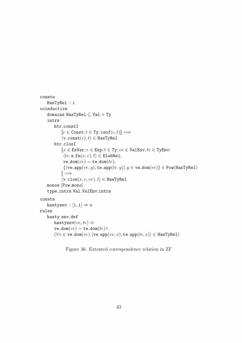
consts

HasTyRel :: icoinductive

domains HasTyRel ⊆ Val× Ty

intrs

htr constI

[[c ∈ Const; t ∈ Ty; isof(c, t)]] =⇒〈v const(c), t〉 ∈ HasTyRel

htr closI

[[x ∈ ExVar; e ∈ Exp; t ∈ Ty; ve ∈ ValEnv; te ∈ TyEnv;〈te, e fn(x, e), t〉 ∈ ElabRel;ve dom(ve) = te dom(te);{〈ve app(ve, y), te app(te, y)〉.y ∈ ve dom(ve)} ∈ Pow(HasTyRel)

]] =⇒〈v clos(x, e, ve), t〉 ∈ HasTyRel

monos [Pow mono]type intrs Val ValEnv.intrs

consts

hastyenv :: [i, i]⇒ o

rules

hasty env def

hastyenv(ve, te) ≡ve dom(ve) = te dom(te)∧(∀x ∈ ve dom(ve).〈ve app(ve, x), te app(te, x)〉 ∈ HasTyRel)

Figure 36: Extented correspondence relation in ZF

43

two rules derived directly from the definition given in the original paper. Thelast premise in the rule for closures (htr closI) is just another way of writing:

∀y ∈ ve dom(ve).〈ve app(ve, y), te app(te, y)〉 ∈ HasTyRel

It was necessary to rewrite the premise, because all premises that mention therecursive set must have the form t ∈M(R), where t is any term, M is a monotoneoperator on sets and R the set under construction. Pow mono is included inthe monos . . . part of the definition because of the monotonicity requirement onM . The rules needed to type-check the definition are the introduction rules forvalues and value environments: Val ValEnv.intrs. The package derives all thenecessary rules: introduction rules, elimination rules and the co-induction rule.Finally the pointwise extension to environments hastyenv is defined.

The formulation of consistency and basic consistency is shown in Figure 37and is exactly the same as in HOL except for the syntax used and the explicittype constraints.

Consistency

〈ve, e, v〉 ∈ EvalRel =⇒(∀t te.hastyenv(ve, te) −→ 〈te, e, t〉 ∈ ElabRel −→ 〈v, t〉 ∈ HasTyRel)

Basic Consistency

[[ ve ∈ ValEnv; te ∈ TyEnv;isofenv(ve, te);〈ve, e, v const(c)〉 ∈ EvalRel;〈te, e, t〉 ∈ ElabRel

]] =⇒isof(c, t)

Figure 37: Consistency in ZF

5.4.2 Proving Consistency

The differences between the formal proof of consistency in HOL and ZF are small.In fact large parts of the proof was mainly done by cutting and pasting from theproof in HOL.

The structure of the proof in ZF is exactly the same as in HOL. Consistencyis proved by induction on the structure of evaluations, by using the inductionrule proved by the (co)inductive package. This leads to six cases, one for eachrule of the inference system. These are all proved more or less the same way asin HOL, using equivalent rules.

44

Size-wise, the two proofs are also very similar. One would expect proofs tobe a bit longer in ZF, because all type constraints must be proved by hand, incontrast to HOL where they are dealt with automatically by the type system ofIsabelle. Even though, it turns out that parts of the proof is actually shorter inZF, because of other improvements, which could also have been made in HOL.For example the first three cases effectively reduces to one line proofs, by usingsome suitable classical reasoning sets. The three remaining cases still requiressome manual effort to get though.

5.5 Discussion

5.5.1 Non-well-founded objects in ZF

As demonstrated above, the choice of the well-founded set theory ZF over non-well-founded set theory or HOL clearly has consequences when dealing with non-well-founded objects. It is not surprising that it is possible to formalise theconsistency result in ZF. At worst one could imagine that it would be necessaryto adopt a finite encoding of non-well-founded closures. It however turned outfar more positive. By using a variant encoding it is possible to work with genuinenon-well-founded objects in ZF. Co-datatypes have a place in ZF.

On the negative side quite a lot of work might be required to define and provethe necessary properties about the variant constructions needed. The example ofvariant maps above clearly illustrates that. It can however largely be put downto lack of support. The theory for ordinary notions such as pairs, functions etc.are far more developed, than the theory for the corresponding variant notions.Even with such a well developed theory some oddities might remain. It is, forexample, necessary to ensure that certain sets used in connection with variantmaps, do not contain the empty set as an element.

There is one issue which have not been addressed here: how to constructnon-well-founded elements. It has not been proved that a theorem similar to(4) actually holds for values. A typical way to prove the “exists” part of such atheorem would be to exhibit a witness and prove that it is a value. This shouldbe done.

5.5.2 The (co)inductive package

There is no question that the (co)inductive package is a big improvement ofIsabelle ZF. Regarding the design of the package, the formalisation of the consis-tency result only gave rise to a few minor points of criticism:

• Generally, definitions and proofs are written in different files in Isabelle.Definitions reside in theory files and proofs in ML files. Theory files andML files belong together pairwise. Isabelle loads a ML file after the cor-responding theory file. Because (co)inductive definitions can refer to rules

45

that requires proof, it is sometimes necessary to do proofs within a theoryfile, which looks rather ugly, or to split the theory file although this is notmotivated by the structure of the development.

• In the case of mutually defined sets, it would be nice to have specialisedelimination rules for each set, instead of only having an elimination for thecombined set. In the case of (co)datatypes it would also be nice to havespecialised case-analysis operators.

• It would be nice if the (co)inductive package could organise the derivedrules into suitable classical reasoning sets. Such sets made the proof ofconsistency easier.

• Although not directly related to the design of the package, a further devel-oped theory of variant functions, products, sums etc. would be very useful.This is especially true when dealing with co-datatypes as the definition ofvalues and value environment above illustrates.

Most of the time the package did exactly what was needed. Without mention-ing it all again, a particular useful feature was the function mk cases for derivingspecial instances of the elimination rules.

The work with the package revealed several bugs. None of these were seri-ous, in the sense that something wrong could be proved. The package does notmerely state axioms, but proves all the necessary rules from definitions. As aconsequence, the errors manifested themselves, as the package not being able toprove some of the rules or looping in the attempt.

6 Conclusion

The main result of the paper [2], consistency, has been proved formally in IsabelleHOL and Isabelle ZF.

The notions of especially inductive definitions and datatypes but also co-inductive definitions and co-datatypes turned out to be central in the formal treat-ment that leads to the consistency result. In Isabelle HOL (co)inductive defini-tions were formalised using a theory of least and greatest fixed points, while an ax-iomatic specification was given of (co)datatypes. In Isabelle ZF all (co)inductivedefinitions and (co)datatypes were formalised using the (co)inductive packageavailable.

The development in Isabelle HOL clearly demonstrated the need for auto-mated support for (co)inductive definitions of sets and datatypes, as an esti-mated 4/5 of the work was related to such definitions. Even more work wouldhave been required if the datatypes had been defined using the fixed point theory.The formalisation in Isabelle ZF confirmed this. The (co)inductive package in

46

ZF reduced the work required dramatically. In many cases the package provedall the rules needed for each (co)inductive definition.

The handling of non-well-founded objects in the well-founded set theory ZF,turned out to be particular interesting. It was possible to represent non-well-founded closures as genuine non-well-founded objects. It was done by using arepresentation based on a so called variant notion of pairs, as opposed to ordinarypairs.

In contrast to HOL, ZF is an untyped logic. In general it made theoremsand proofs slightly bigger in HOL. It however did not have any real practicalconsequences. Quite the opposite, much of the development in ZF was done bycutting and pasting from the corresponding parts in the HOL development.

Doing the actual consistency proof in both Isabelle HOL and ZF was a verypositive experience. In both cases it proceeded more or less as the original proofand hardly required any knowledge of how consistency originally was proved.Difficulties only arose, when the original proof was not as clear as one couldwish. It seems that the hard part is to do the proof, not to formalise it. Quiteremarkable it only require about the same space as its more informal counterpart.This contradicts what seems to be the common conception, that formal proofsnecessarily are long and much harder to do than the corresponding informal ones.

Acknowledgements. Lawrence C. Paulson suggested the project and gavemuch useful advice. Søren T. Heilmann, Niels B. Maretti and Ole Rasmussencommented on drafts of this paper or its predecessor. Mads Tofte answered ques-tions about his and Robin Milner’s paper.

References

[1] Jacob Frost. A case study of co-induction in Isabelle HOL. Tech-nical Report 308, University of Cambridge, Computer Laboratory, Au-gust 1993. http://www.cl.cam.ac.uk/Research/Reports/TR308-jf10008-co-induction.dvi.gz.

[2] Robin Milner and Mads Tofte. Co-induction in relational semantics. Theo-retical Computer Science, 87:209–220, 1991.

[3] Lawrence C. Paulson. Co-induction and co-recursion in higher-orderlogic. Technical Report 304, University of Cambridge, Computer Labo-ratory, July 1993. http://www.cl.cam.ac.uk/Research/Reports/TR304-lcp-coinduction.ps.gz.

[4] Lawrence C. Paulson. Introduction to Isabelle. Technical Report 280,University of Cambridge, Computer Laboratory, January 1993. ftp://ftp.cl.cam.ac.uk/ml/intro.dvi.gz.

47

[5] Lawrence C. Paulson. The Isabelle reference manual. Technical Report 283,University of Cambridge, Computer Laboratory, February 1993. ftp://ftp.cl.cam.ac.uk/ml/ref.dvi.gz.

[6] Lawrence C. Paulson. A concrete final coalgebra theorem for ZF set the-ory. Technical Report 334, University of Cambridge, Computer Labora-tory, May 1994. http://www.cl.cam.ac.uk/Research/Reports/TR334-lcp-final.coalgebra.dvi.gz.

[7] Lawrence C. Paulson. A fixedpoint approach to implementing (co)inductivedefinitions. Technical Report 320, University of Cambridge, ComputerLaboratory, November 1994. http://www.cl.cam.ac.uk/Research/Reports/TR320-lcp-isabelle-ind-defs.dvi.gz.

[8] Lawrence C. Paulson. Isabelle, A Generic Theorem Prover. Number 828 inLecture Notes in Computer Science. Springer-Verlag, Berlin, 1994.

[9] Lawrence C. Paulson. Isabelle’s object-logics. Technical Report 286, Uni-versity of Cambridge, Computer Laboratory, October 1994. ftp://ftp.Cl.cam.ac.uk/ml/logics.dvi.gz.

[10] Tobias Nipkow and Lawrence C. Paulson. Datatypes and (co)inductive def-initions in Isabelle/HOL. ftp://ftp.cl.cam.ac.uk/ml/HOL-extensions.dvi.gz,1994.

48

a case study of co-induction in isabelle 1 · a case study of co-induction in isabelle 1 jacob...

Documents