919 decompositionofforcedturbulentjetﬂows -...

919

Decomposition of forced turbulent jet flowsA Erdil1∗, H M Ertunc1, and T Yilmaz2

1Mechatronics Engineering Department, Kocaeli University, Izmit, Turkey2Department of Naval Architecture, Yıldız Technical University, Istanbul, Turkey

The manuscript was received on 7 May 2008 and was accepted after revision for publication on 27 August 2008.

DOI: 10.1243/09544062JMES1173

Abstract: In many cases, turbulence is superimposed on an unsteady organized motion of amean flow. Indeed, large ranges of scales are involved in these flows, and it is important to inves-tigate their characteristics and interactions. Thus, the time–frequency decomposition providedby the wavelet analysis appears an efficient tool that complements the classical approach andthe Fourier transform. In this study, the wavelet decomposition (WD) method has been appliedto the forced turbulent jet flows. The obtained results of the WD are compared with those of theother most common techniques such as proper orthogonal decomposition and phase averaging.In addition, the spectrogram of the signals has been presented for a visual representation of thefrequency contents. It is shown that theWD is a successful tool to decompose the forced turbulentjet flows into its components for various axial distances, Re numbers, and forcing frequencies.

Keywords: turbulence, forced jet flows, wavelet decomposition

1 INTRODUCTION

The forced turbulent jet flows are used in many indus-trial applications such as convection heat transferand combustion [1, 2]. In these flows, various meth-ods are used to decompose the measured velocityinto organized and turbulent motions. Some of thedecomposition methods are high-pass filtering [3],phase averaging [4], conditional averaging [5], quad-rant analysis [6], and proper orthogonal decompo-sition (POD) [7]. Several of these methods requiresome information about the flow to determine theturbulent and organized components. The phase aver-aging method is appropriate for the flows in whichthe organized unsteady motion is identically repeatedfrom cycle to cycle, and the turbulent motions in suc-cessive cycles are considered as independent events.So, this decomposition method has been widely usedin the forced and naturally unsteady flows [8–10].If the cycle period is known precisely and cycle-to-cycle variations in organized motions are negligible,this technique recovers accurate results. In many fluidflows, the cycle period cannot be specified with suf-ficient accuracy, and cycle-to-cycle variations of the

∗Corresponding author: Mechatronics Engineering Department,

Kocaeli University,Umuttepe Campus,Kocaeli 41380,Izmit,Turkey.

email: [email protected]

organized motions are not negligible. Therefore, thesubharmonic motions and organized motions will bemisrepresented as turbulence. The high pass filteringmethod is strongly affected by the arbitrary selectionof cut-off frequency [3]. This may result in an under-estimation of turbulence magnitudes by removing allenergy content below the cut-off frequency.

The problem of the response of a jet to periodicexcitations has attracted considerable interest frommany researchers, mainly because of its fundamen-tal importance in the problem of flow instability andalso of its practical implications in noise and/or turbu-lence reduction and in enhanced mixing or spreadingrate. It is well-known that these phenomena are closelyrelated to the behaviour of initially rolled-up vorticesin the free-shear-layer part of the jet, and hence maypossibly influence the large-scale coherent structureof the turbulent jet downstream. Zaman and Hus-sain [11, 12] have made comprehensive studies in thisdirection.

In recent years, the wavelet transform is used as aneffective tool to investigate the turbulent flow fields.The time–frequency distributions of axial turbulencevelocities of spiral pipe flow is decomposed fromlow frequency level (low wave number) to high fre-quency level (high wave number) by means of discretewavelet transform (DWT) and its autocorrelation, asin Takei et al. [13]. As a result, the fluctuation lev-els of spiral flow are extremely low as compared with

JMES1173 © IMechE 2009 Proc. IMechE Vol. 223 Part C: J. Mechanical Engineering Science

920 A Erdil, H M Ertunc, and T Yilmaz

those of the typical turbulent flow. Camussi [14] inves-tigated the bi-dimensional velocity fields to extractand characterize the swirling motion associated withcoherent structures by using a new technique basedon the wavelet transform. The technique proposedmakes it possible to analyse some aspects that arepartially missed by other identification methodolo-gies. Accounting for the strong differences among theexamined test cases, it is argued that a successfulapplication of the present procedure might not beaffected either by the methodology used for the extrac-tion of the velocity vector field or the type of flow ana-lysed. Farge et al. [15] investigated the turbulent flows’decomposition into two orthogonal parts: a coher-ent, inhomogeneous, non-Gaussian component andan incoherent, homogeneous, Gaussian component.This decomposition process was carried out by usinga non-linear scheme based on an objective thresholddefined in terms of the wavelet coefficients of the vor-ticity. They proposed a new method called coherentvortex simulation designed to compute and modelthe two-dimensional turbulent flows by using theprevious wavelet decomposition (WD) at each timestep.

Some of the previous works on the coherent struc-tures identification has focused the application ofseveral methods. Sullivan and Pollard [16] investigatedthe identification of coherent structures from multi-point measurements made in a three-dimensionalwall jet by using different methods: POD, linearstochastic estimation, Gram–Charlier estimation, andWD. After applying these methods, they analysed theresulting information to extract the structure. Theyproposed that the anisotropic growth rate (i.e. fasterspreading in the lateral direction in comparison to thetransverse direction) found in the wall jet is due tolarge-scale structure. Bonnet et al. [17] investigated tovalidate, test, and compare by using several coherentstructure eduction methods (such as POD, the waveletanalysis, and the ensemble average methods) utilizingthe same database. They found that direct compar-isons between the results of several methods arepossible. Good quantitative and qualitative agreementbetween the different methods has been observedas well as some differences noted. Kodal et al. [18]investigated PIV measurements lifted CH4-air diffu-sion flames at three different Reynolds numbers byusing the turbulence filter and the POD methods. Theyreported that the first modes (mean flow) comprise 85per cent of the total energy.

The objective of this article is to decompose theforced turbulent jet flows by using the wavelet trans-form. The decomposed organized motions obtainedby the wavelet transform are compared with the resultsof POD and phase averaging methods in both timeand frequency domain. Besides, the spectrogram ofthe signals has been presented for a visual representa-tion of the frequency contents. Among the methods,

the wavelet transform has emerged as a time-scaleanalysis method for non-stationary signal processing.Basically, the wavelet transform is the decomposi-tion of arbitrary signals into localized contributionslabelled by a scale parameter. Therefore, it is capableof representing the temporal characteristics of a signalby its spectral components in the frequency domain.Because of this feature, it has found important appli-cations in many areas such as data compression, videocoding multi-resolution techniques, edge detection,speech recognition, image processing, tool condi-tion monitoring, and especially for biomedical signalprocessing [19, 20].

2 EXPERIMENTAL SET-UP

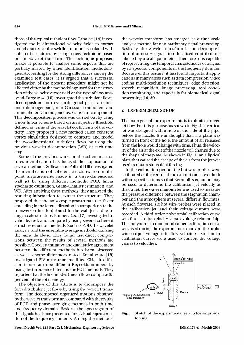
The main goal of the experiments is to obtain a forcedjet flow. For this purpose, as shown in Fig. 1, a verticaljet was designed with a hole at the side of the pipe,before the nozzle. It was thought that, if a plate wasturned in front of the hole, the amount of air releasedfrom the hole would change with time. Thus, the veloc-ity of the air at the exit of the nozzle will change due tothe shape of the plate. As shown in Fig. 1, an ellipticalplate that caused the escape of the air from the jet wasused to obtain sinusoidal forcing.

In the calibration period, the hot wire probes werecalibrated at the centre of the calibration jet exit builtwithin specifications so that Bernoulli’s equation maybe used to determine the calibration jet velocity atthe outlet. The water manometer was used to measurethe pressure difference between the stagnation cham-ber and the atmosphere at several different flowrates.At each flowrate, six hot wire probes were placed inthe calibration jet, and their voltage outputs wererecorded. A third-order polynomial calibration curvewas fitted to the velocity versus voltage relationship.This polynomial equation obtained calibration curvewas used during the experiments to convert the probewire output voltage into flow velocities. Six similarcalibration curves were used to convert the voltagevalues to velocities.

Fig. 1 Sketch of the experimental set-up for sinusoidalforcing

Proc. IMechE Vol. 223 Part C: J. Mechanical Engineering Science JMES1173 © IMechE 2009

Decomposition of forced turbulent jet flows 921

After the calibration procedure, the sinusoidalforced turbulent jet flow measurements were carriedout for different test cases in the experiment. In theexperiment, the channel number (hot wire number) issix, data number 10 000, and the sampling frequency13 kHz. A relative time was assigned to each velocitymeasurement because the data were acquired at aknown frequency (the sampling frequency) of our A/Dcard. As the first test case, the forced motion was alsomeasured at different axial distances between 3 and18d, where d is the diameter of the nozzle. For thesecond test case, the Re number was varied between6000 and 19 000; and, finally, for the third test case, theforcing frequency was chosen as 60, 80, 100, 120, and140 Hz. A photo detector measured the frequency ofthe plate. Two sinus cycles were obtained for one rev-olution of the plate. To generate the forcing flow, theplate was driven by a DC electric motor that has maxi-mum speed of 4500 r/min. Thus, the forcing frequencyof the organized motion was two times the frequencyof the turning plate.

3 MATHEMATICAL BACKGROUND

3.1 Wavelet decomposition

The spectral analysis and time series method are themost commonly used signal processing techniques inengineering. The Fourier transform (FT), one of themost known and oldest signal-processing tools forlong years, provides information about the frequencycontents and/or spectral components of the signal.The FT decomposes a signal into constituent sinu-soids of different frequencies that can be shown bycomplex exponentials. Since it does not provide anytime information, it is not possible to find out whena particular event occurs. Therefore, this is the majordrawback of the FTs. To overcome this drawback, thesignal is broken up to contiguous segments and theFT of each segment is taken separately. The short timeFourier transform (STFT) is similar to this procedure.In the STFT, the function x(t) is multiplied by a win-dow function w(t), and the FT is calculated. Then thewindow function is shifted by τ in time, and the FT iscalculated again.

The drawback with the STFT is the necessity ofchoosing a particular size for the window. Due tothe uncertainty principle, one cannot know the exacttime–frequency representation of a signal, i.e. one can-not know what spectral components exist at whichinstances of time. What one can know is the timeintervals in which a certain band of frequencies exist,which is a resolution problem.

As an alternative approach to the STFT, to over-come the resolution problem and to provide goodlocalization of signal discontinuities that is requiredfor the analysis of non-stationary signals, the wavelets

are introduced as a signal representation. When pass-ing through a signal, the analysis window’s size ofa wavelet is chosen to be short at high frequenciesand long at low frequencies to pick up all the abruptchanges. In this way, it is possible to represent thetemporal characteristics of a signal by its spectralcomponents in the frequency domain.

The wavelet analysis is done in a similar way to theSTFT analysis, in the sense that the signal is multipliedwith a particular function that is the wavelet function,similar to the window function in the STFT; and thetransform is computed separately for different seg-ments of the time-domain signal. The main purpose ofthe wavelet transform is to decompose any signal intoa set of basis functions that can be labelled by a scalethe parameter. This enables the analysis of a localizedarea of a larger signal. The basis functions are obtainedby dilations, contractions, and shifts of a unique func-tion called the mother (or original) wavelet. In otherwords, the wavelet analysis is the breaking up of anysignal into shifted and scaled versions of the motherwavelet. Indeed, the wavelet is a waveform of effec-tively limited duration that has an average value ofzero.

For a given discrete time signal, the DWT is definedas

XDWT(k, n) =∫∞

−∞x(t)2−k/2ψ∗(2−kt − nT ) dt (1)

In this equation, ψ is the basis function called themother wavelet in which * denotes a complex conjuga-tion, 2knT is the position of the wavelet function in thediscrete time domain, and 2k is the scaling factor. Here,T is the sampling time (one can assume sampling timeT = 1 without loss of generality); and k and n the inte-ger numbers. Since all signal-processing techniquesare performed on a computer nowadays, the transformtechniques, therefore, must be performed on discretesignals. For this reason, the first step to computing theDWT is the discretization of a given continuous timeinput signal x(t). A fast wavelet transform was devel-oped based on the Mallat pyramidal algorithm, alsoknown as two-channel subband coder, for computerapplications [21].

The main idea in the DWT is to obtain a time-scale representation of a digital signal by using thedigital filtering techniques. In other words, filters ofdifferent cut-off frequencies are used to analyse thesignal at different scales. The signal is passed througha series of high pass filters to analyse the high fre-quencies, and it is passed through a series of low passfilters to analyse the low frequencies. Thus, the DWTanalyses the signal at different frequency bands withdifferent resolutions by decomposing the signal intoa coarse approximation and detail information. TheDWT employs two sets of functions, called scalingfunctions and wavelet functions, which are associated



with low-pass and high-pass filters, respectively. Thedecomposition of the signal into different frequencybands is simply obtained by successive high-pass andlow-pass filtering of the time domain signal.

The wavelet analysis is a decomposition of thesignal on a family of analysing signals, which is usu-ally an orthogonal function method. On the otherhand, the wavelet analysis offers a harmonious com-promise between the decomposition and smoothingtechniques. In this study, the turbulent jet velocitysignals were decomposed into a hierarchical set ofapproximations and details by using the wavelet anal-ysis. The selection of a suitable level for the hierarchywill depend on the signal and experience. Level 6 waschosen for decomposing the organized motion fromturbulence.

First, the DC part of the raw signal is removed andthe left signal is called the total signal. The total signal,now, consists of the organized and turbulent motion asexplained in the introduction section. These parts cor-respond to approximation and details in the waveletliterature. In other words, the approximation or orga-nized motion takes into account the low frequencies ofthe total signal, whereas the summation of all detailscorresponds to the high frequency correction. Appar-ently, the total signal can be reconstructed from theapproximation and details.

3.2 POD method

Lumley proposed describing the random fields suchas turbulence as deterministic functions that are asnearly parallel as to u, the ensemble vector of thefield [7]. In the statistical sense, the modulus square ofthe product of the vector and deterministic functionare maximized

〈(ui, k)2〉‖k‖2

!= Max (2)

where the symbol ‖.‖ is used for the norm

‖k‖2 = (k, k) (3)

where (k, k) represent the inner product of two vectorfunctions. This representation problem leads to theequation

∫+∞

−∞Ruu(t , t ′)k(t ′) dt ′ = λk(t) (4)

where Ruu(t , t ′) is a time-delayed correlation func-tion, k(t ′) is the deterministic eigenvector, and λ thecorresponding eigenvalue. Each eigenmode of thedecomposition can be expressed as

ui = (u, ki)ki (5)

Each eigenmode can be considered as representinga coherent structure (or some orthogonal contribution

to a coherent structure). The ensemble vector u can beresolved as

u =∞∑

i=1

(u, ki)ki (6)

which is the sum of all orthogonal modes, which Lum-ley called the characteristic eddies. The significance ofthis decomposition is that its modes constitute a spe-cial basis, which is an optimal set in the sense thatwhen truncated at any arbitrary number of modes, noother decomposition truncated at the same order cancapture a greater fraction of the energy of the dataseries. The percentage of the total energy containedin the ith energy mode (activation ratio) can be foundusing

�i = λi∑∞j=1 λj

(7)

where �i is the ‘activation’ of the ith mode.For the low Reynolds number flows, a large por-

tion of the energy is often contained in relativelyfew modes [22, 23], so that the coherent structuresare easily detectable and may be identified by thisdecomposition.

3.3 Phase averaging technique

Following the decomposition method proposed byHussain and Reynolds [4], any organized unsteady tur-bulent flow variable f (x, t) can be decomposed intothree parts with respect to their characteristic timedependence

f (x, t) = f (x) + f (x, t) + f ′(x, t) (8)

When the organization is known to be cyclic intime, the mean or the time-averaged component isconventionally defined as

f (x) = limN→∞

1N

N−1∑

n=0

f (x, t0 + n�t) where N�t τ

(9)

where τ is the period of the cycle. The organizedunsteady component can be calculated by averagingat the same phase in each cycle

f (x) + f (x, t) = 〈 f (x, t)〉 = limN→∞

1N

N−1∑

n=0

f (x, t + nτ)

(10)

The phase-averaged and turbulent componentsare by definition uncorrelated in time, so it



follows that: f ′(x, t) = f (x, t) − 〈 f (x, t)〉 and f (x, t) =〈 f (x, t)〉 − 〈 f (x, t)〉. If τ t , the cycle period, is knownprecisely and the cycle-to-cycle variations of theorganized motion are negligible, then this techniquerecovers accurate results.

3.4 Spectrogram

The spectrogram is a visual representation of STFT.Recall that STFT is the discrete-time FT for a sequence,computed by using a sliding window that is explainedin section 3.1. Similarly, by using a sliding window, thespectrogram of a signal is found to compute the mag-nitude of the time-dependent FT versus time. The timegoes from left to right, with frequency representedvertically. Note that the resolution of the spectro-gram of a signal depends on the size of the Fourieranalysis window. A long window resolves frequencyat the expense of time; the result is a narrowbandspectrogram, which reveals the individual harmonics(component frequencies). If a small analysis windowis used, the adjacent harmonics are smeared together,but with better time resolution.

The frequency content of the signal is representedby different intensities of red, green, and blue colours.The higher spectra are more energetic signals; thedarker colour (dark red) is used in the representa-tion. If a signal has a fundamental harmonic at alllengths, that frequency will be shown as a colouredline in the spectrogram figure. The instantaneous highfrequency components appear as a darker red colourassociated with a resolution determined by the size ofthe window.

From the mathematical point of view, the continu-ous time spectrogram is defined as

Sf (n, �) =∣∣∣∣∫

τ

e−jωτ f (τ )h(τ − t) dτ

∣∣∣∣2

(11)

where h(τ ) is a window function. On the other hand,the spectrogram of a discrete-time signal, f [k], isdefined as

Sf [n, �] =∣∣∣∣∣∑

k

e−j�kf [k]h[k − n]∣∣∣∣∣

2

(12)

where n is the discrete-time instant [24]. One notesthat the spectrogram expressed in equation (12) isperiodic in �.

4 RESULTS AND DISCUSSION

Although the experiments were carried out for sixchannels, only the signals at the centre-line of theforced jet were considered for decomposition in thisstudy. Several test cases were carried out by changingthe values of axial distances, Reynolds numbers, andforcing frequencies.

4.1 Various axial distances using WD method

In the first test case, the forced turbulent jet flow wasinvestigated for various axial distances, i.e. z/d = 3,6, 9, 12, 15, and 18 at the centre of forced jet. Here,z is the distance along the nozzle axis and d thediameter of the nozzle. The main objective in this test

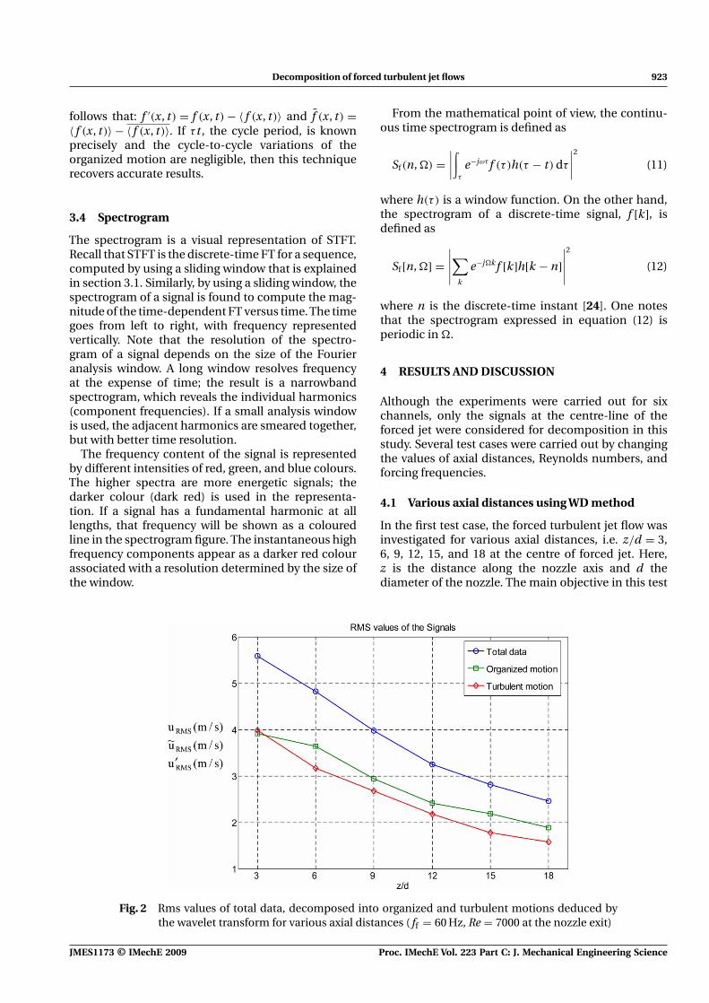
Fig. 2 Rms values of total data, decomposed into organized and turbulent motions deduced bythe wavelet transform for various axial distances ( ff = 60 Hz, Re = 7000 at the nozzle exit)



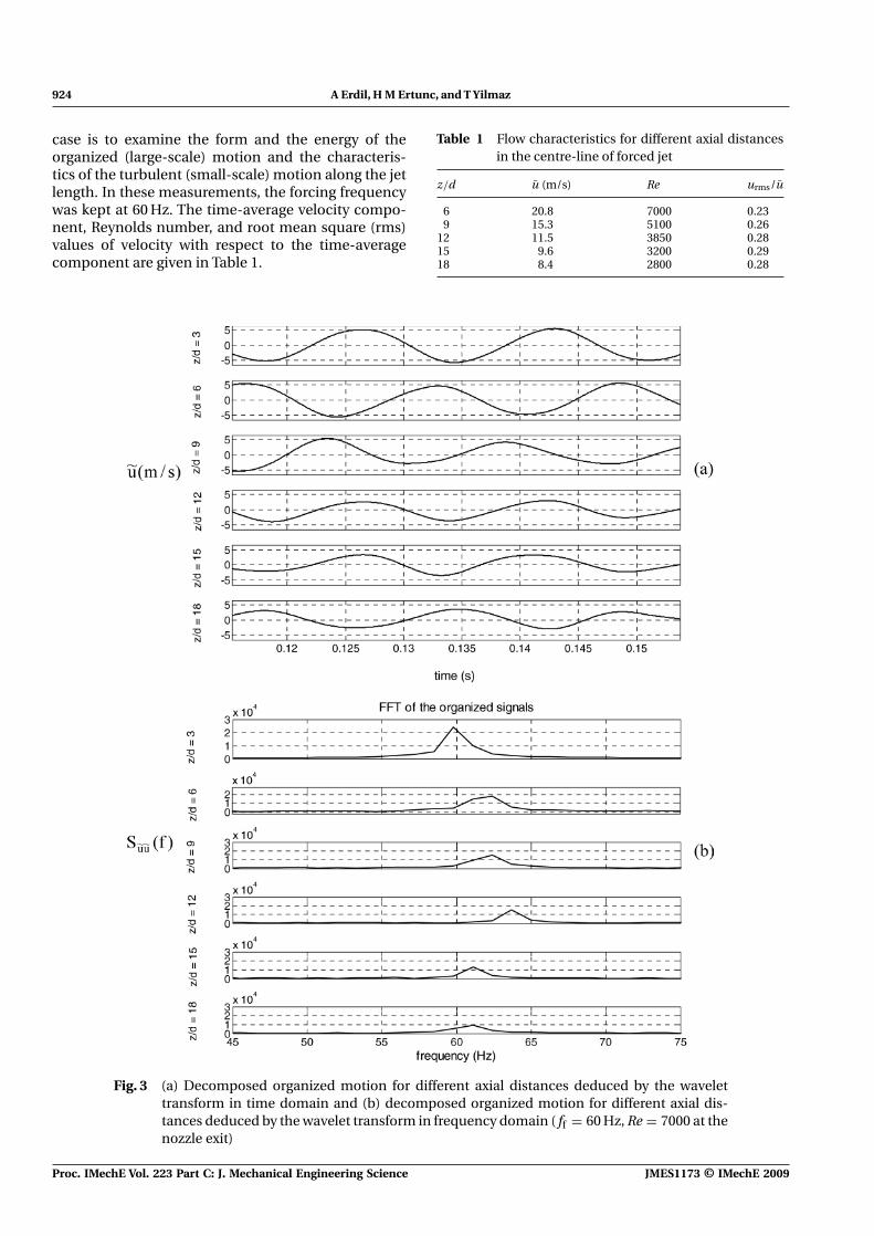
case is to examine the form and the energy of theorganized (large-scale) motion and the characteris-tics of the turbulent (small-scale) motion along the jetlength. In these measurements, the forcing frequencywas kept at 60 Hz. The time-average velocity compo-nent, Reynolds number, and root mean square (rms)values of velocity with respect to the time-averagecomponent are given in Table 1.

Table 1 Flow characteristics for different axial distancesin the centre-line of forced jet

z/d u (m/s) Re urms/u

6 20.8 7000 0.239 15.3 5100 0.26

12 11.5 3850 0.2815 9.6 3200 0.2918 8.4 2800 0.28

Fig. 3 (a) Decomposed organized motion for different axial distances deduced by the wavelettransform in time domain and (b) decomposed organized motion for different axial dis-tances deduced by the wavelet transform in frequency domain ( ff = 60 Hz, Re = 7000 at thenozzle exit)



When the total velocity data series at vari-ous axial distances are decomposed by using thewavelet transform, the organized and turbulentmotions are obtained. The decomposition is per-formed by using the Daubechies 10 (db10) waveletat level 6 [25]. The rms values of the total dataand their decomposed components are plottedwith respect to the axial distance, z/d, in Fig. 2.As shown in this figure, the rms values of thetotal, organized, and turbulent motions decrease

with increasing axial distance in the centre-line offorced jet.

In Fig. 3, the decomposed organized signals usingWD for different axial distances are shown in both timeand frequency domains. It can be seen from the figurethat the amplitude of the time series and spectrummagnitudes of the forced organized motions decreasewith increasing axial distance. This result is very trivialbecause the energy of the signals decreases as thesignals move away from the nozzle.

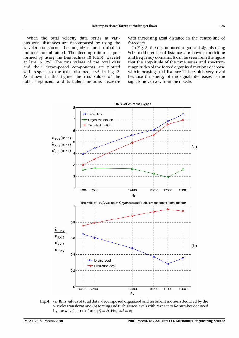
Fig. 4 (a) Rms values of total data, decomposed organized and turbulent motions deduced by thewavelet transform and (b) forcing and turbulence levels with respect to Re number deducedby the wavelet transform ( ff = 80 Hz, z/d = 6)



4.2 Various Reynolds numbers usingWD method

In the second test case, a constant forcing frequencyof 80 Hz was chosen and the experiments were car-ried out at a vertical distance of 30 mm (z/d = 6) atRe numbers of 6000, 7500, 12 400, 15 200, 17 000, and19 000 in the centre-line of the forced jet. In Table 2, thetime average velocity component, Reynolds number,and rms values of the total signal with respect to timeaverage component are given.

In Fig. 4(a), the rms values of the total data, decom-posed organized and turbulent motions are shownwith respect to the Re number. When the Re numberincreases, the rms values of the organized componentare approximately constant, whereas that of the totaldata and the decomposed turbulent motion increases.On the other hand, Fig. 4(b) shows the ratio of rmsvalues of the organized and turbulent motion to thetotal motion with respect to the Re number. While theratio of the organized motion to the total motion is

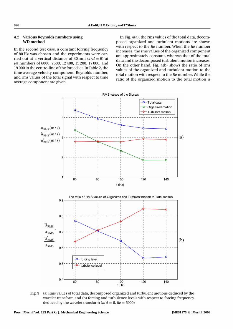
Fig. 5 (a) Rms values of total data, decomposed organized and turbulent motions deduced by thewavelet transform and (b) forcing and turbulence levels with respect to forcing frequencydeduced by the wavelet transform (z/d = 6, Re = 6000)



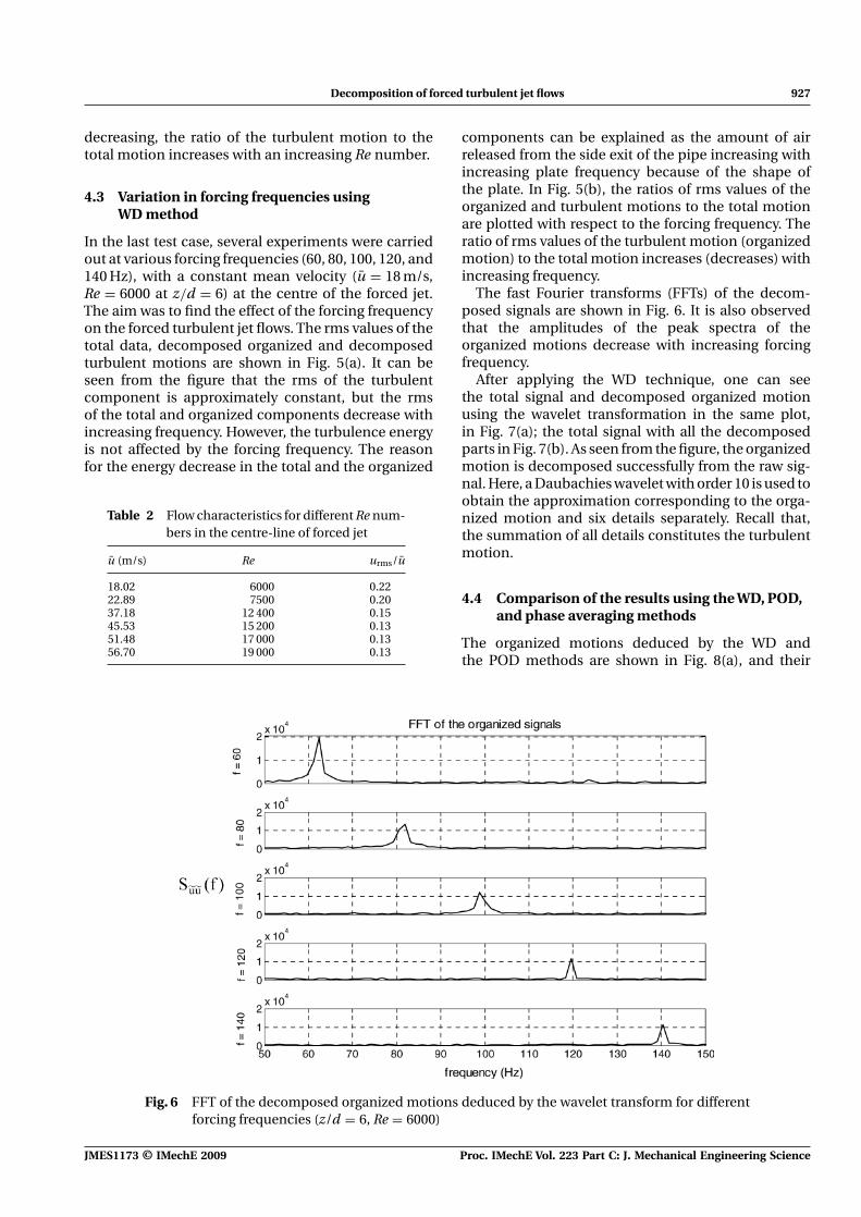
decreasing, the ratio of the turbulent motion to thetotal motion increases with an increasing Re number.

4.3 Variation in forcing frequencies usingWD method

In the last test case, several experiments were carriedout at various forcing frequencies (60, 80, 100, 120, and140 Hz), with a constant mean velocity (u = 18 m/s,Re = 6000 at z/d = 6) at the centre of the forced jet.The aim was to find the effect of the forcing frequencyon the forced turbulent jet flows. The rms values of thetotal data, decomposed organized and decomposedturbulent motions are shown in Fig. 5(a). It can beseen from the figure that the rms of the turbulentcomponent is approximately constant, but the rmsof the total and organized components decrease withincreasing frequency. However, the turbulence energyis not affected by the forcing frequency. The reasonfor the energy decrease in the total and the organized

Table 2 Flow characteristics for different Re num-bers in the centre-line of forced jet

u (m/s) Re urms/u

18.02 6000 0.2222.89 7500 0.2037.18 12 400 0.1545.53 15 200 0.1351.48 17 000 0.1356.70 19 000 0.13

components can be explained as the amount of airreleased from the side exit of the pipe increasing withincreasing plate frequency because of the shape ofthe plate. In Fig. 5(b), the ratios of rms values of theorganized and turbulent motions to the total motionare plotted with respect to the forcing frequency. Theratio of rms values of the turbulent motion (organizedmotion) to the total motion increases (decreases) withincreasing frequency.

The fast Fourier transforms (FFTs) of the decom-posed signals are shown in Fig. 6. It is also observedthat the amplitudes of the peak spectra of theorganized motions decrease with increasing forcingfrequency.

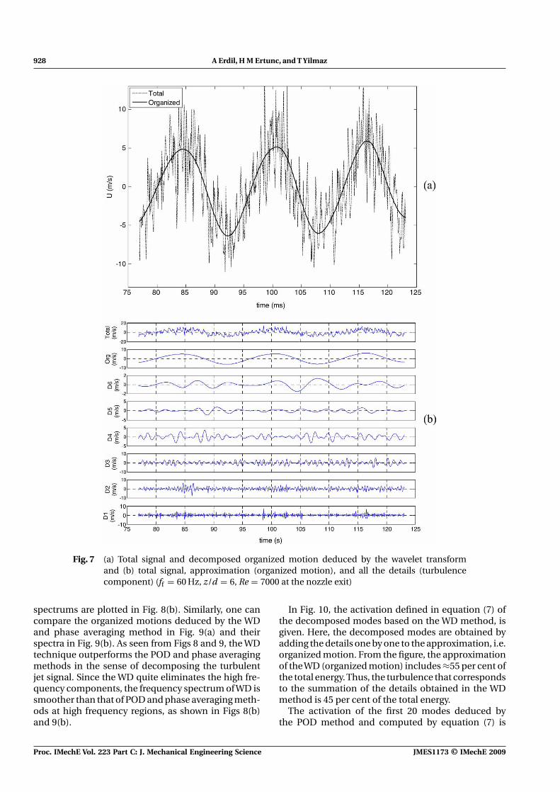
After applying the WD technique, one can seethe total signal and decomposed organized motionusing the wavelet transformation in the same plot,in Fig. 7(a); the total signal with all the decomposedparts in Fig. 7(b). As seen from the figure, the organizedmotion is decomposed successfully from the raw sig-nal. Here, a Daubachies wavelet with order 10 is used toobtain the approximation corresponding to the orga-nized motion and six details separately. Recall that,the summation of all details constitutes the turbulentmotion.

4.4 Comparison of the results using the WD, POD,and phase averaging methods

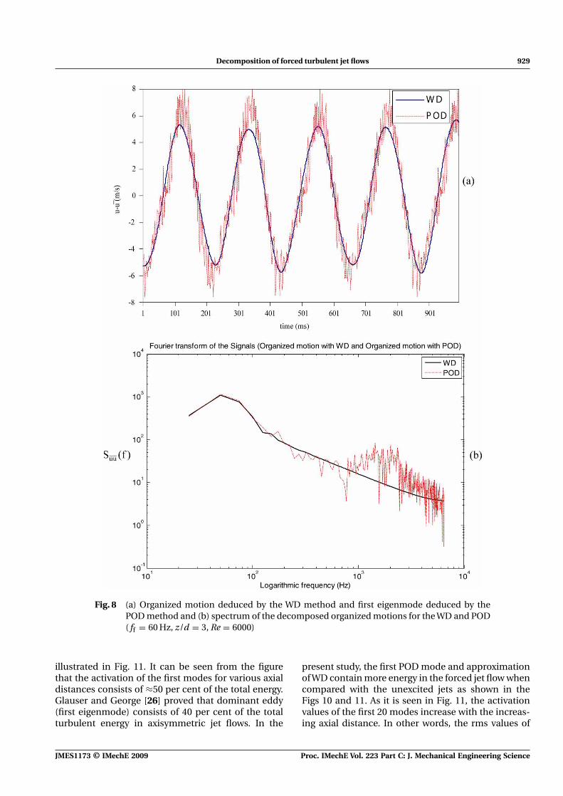
The organized motions deduced by the WD andthe POD methods are shown in Fig. 8(a), and their

Fig. 6 FFT of the decomposed organized motions deduced by the wavelet transform for differentforcing frequencies (z/d = 6, Re = 6000)



Fig. 7 (a) Total signal and decomposed organized motion deduced by the wavelet transformand (b) total signal, approximation (organized motion), and all the details (turbulencecomponent) (ff = 60 Hz, z/d = 6, Re = 7000 at the nozzle exit)

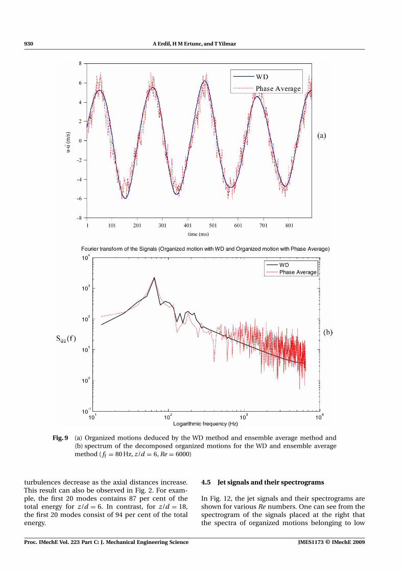
spectrums are plotted in Fig. 8(b). Similarly, one cancompare the organized motions deduced by the WDand phase averaging method in Fig. 9(a) and theirspectra in Fig. 9(b). As seen from Figs 8 and 9, the WDtechnique outperforms the POD and phase averagingmethods in the sense of decomposing the turbulentjet signal. Since the WD quite eliminates the high fre-quency components, the frequency spectrum of WD issmoother than that of POD and phase averaging meth-ods at high frequency regions, as shown in Figs 8(b)and 9(b).

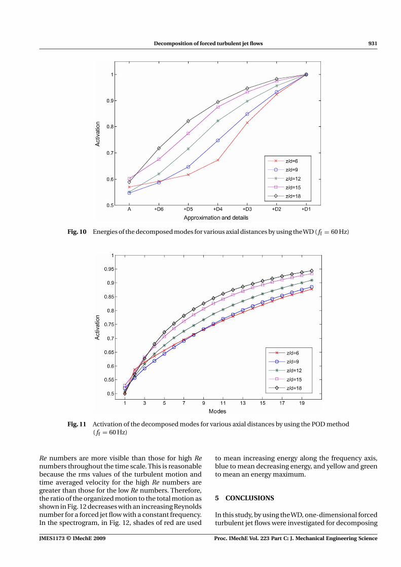
In Fig. 10, the activation defined in equation (7) ofthe decomposed modes based on the WD method, isgiven. Here, the decomposed modes are obtained byadding the details one by one to the approximation, i.e.organized motion. From the figure, the approximationof the WD (organized motion) includes ≈55 per cent ofthe total energy. Thus, the turbulence that correspondsto the summation of the details obtained in the WDmethod is 45 per cent of the total energy.

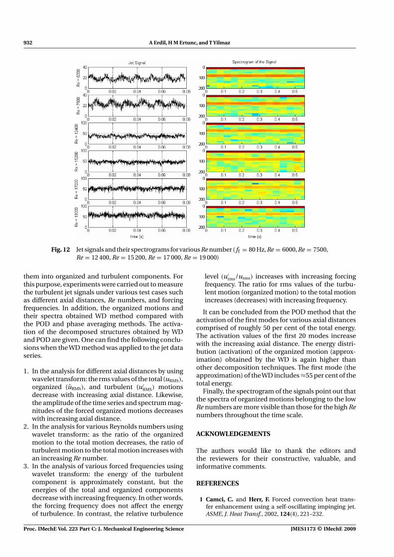
The activation of the first 20 modes deduced bythe POD method and computed by equation (7) is



Fig. 8 (a) Organized motion deduced by the WD method and first eigenmode deduced by thePOD method and (b) spectrum of the decomposed organized motions for the WD and POD( ff = 60 Hz, z/d = 3, Re = 6000)

illustrated in Fig. 11. It can be seen from the figurethat the activation of the first modes for various axialdistances consists of ≈50 per cent of the total energy.Glauser and George [26] proved that dominant eddy(first eigenmode) consists of 40 per cent of the totalturbulent energy in axisymmetric jet flows. In the

present study, the first POD mode and approximationof WD contain more energy in the forced jet flow whencompared with the unexcited jets as shown in theFigs 10 and 11. As it is seen in Fig. 11, the activationvalues of the first 20 modes increase with the increas-ing axial distance. In other words, the rms values of



Fig. 9 (a) Organized motions deduced by the WD method and ensemble average method and(b) spectrum of the decomposed organized motions for the WD and ensemble averagemethod ( ff = 80 Hz, z/d = 6, Re = 6000)

turbulences decrease as the axial distances increase.This result can also be observed in Fig. 2. For exam-ple, the first 20 modes contains 87 per cent of thetotal energy for z/d = 6. In contrast, for z/d = 18,the first 20 modes consist of 94 per cent of the totalenergy.

4.5 Jet signals and their spectrograms

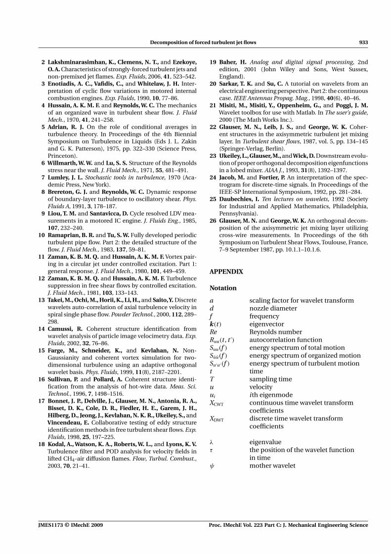
In Fig. 12, the jet signals and their spectrograms areshown for various Re numbers. One can see from thespectrogram of the signals placed at the right thatthe spectra of organized motions belonging to low



Fig. 10 Energies of the decomposed modes for various axial distances by using theWD ( ff = 60 Hz)

Fig. 11 Activation of the decomposed modes for various axial distances by using the POD method( ff = 60 Hz)

Re numbers are more visible than those for high Renumbers throughout the time scale. This is reasonablebecause the rms values of the turbulent motion andtime averaged velocity for the high Re numbers aregreater than those for the low Re numbers. Therefore,the ratio of the organized motion to the total motion asshown in Fig. 12 decreases with an increasing Reynoldsnumber for a forced jet flow with a constant frequency.In the spectrogram, in Fig. 12, shades of red are used

to mean increasing energy along the frequency axis,blue to mean decreasing energy, and yellow and greento mean an energy maximum.

5 CONCLUSIONS

In this study, by using theWD, one-dimensional forcedturbulent jet flows were investigated for decomposing



Fig. 12 Jet signals and their spectrograms for various Re number ( ff = 80 Hz, Re = 6000, Re = 7500,Re = 12 400, Re = 15 200, Re = 17 000, Re = 19 000)

them into organized and turbulent components. Forthis purpose, experiments were carried out to measurethe turbulent jet signals under various test cases suchas different axial distances, Re numbers, and forcingfrequencies. In addition, the organized motions andtheir spectra obtained WD method compared withthe POD and phase averaging methods. The activa-tion of the decomposed structures obtained by WDand POD are given. One can find the following conclu-sions when the WD method was applied to the jet dataseries.

1. In the analysis for different axial distances by usingwavelet transform: the rms values of the total (uRMS),organized (uRMS), and turbulent (u′

RMS) motionsdecrease with increasing axial distance. Likewise,the amplitude of the time series and spectrum mag-nitudes of the forced organized motions decreaseswith increasing axial distance.

2. In the analysis for various Reynolds numbers usingwavelet transform: as the ratio of the organizedmotion to the total motion decreases, the ratio ofturbulent motion to the total motion increases withan increasing Re number.

3. In the analysis of various forced frequencies usingwavelet transform: the energy of the turbulentcomponent is approximately constant, but theenergies of the total and organized componentsdecrease with increasing frequency. In other words,the forcing frequency does not affect the energyof turbulence. In contrast, the relative turbulence

level (u′rms/urms) increases with increasing forcing

frequency. The ratio for rms values of the turbu-lent motion (organized motion) to the total motionincreases (decreases) with increasing frequency.

It can be concluded from the POD method that theactivation of the first modes for various axial distancescomprised of roughly 50 per cent of the total energy.The activation values of the first 20 modes increasewith the increasing axial distance. The energy distri-bution (activation) of the organized motion (approx-imation) obtained by the WD is again higher thanother decomposition techniques. The first mode (theapproximation) of the WD includes ≈55 per cent of thetotal energy.

Finally, the spectrogram of the signals point out thatthe spectra of organized motions belonging to the lowRe numbers are more visible than those for the high Renumbers throughout the time scale.

ACKNOWLEDGEMENTS

The authors would like to thank the editors andthe reviewers for their constructive, valuable, andinformative comments.

REFERENCES

1 Camci, C. and Herr, F. Forced convection heat trans-fer enhancement using a self-oscillating impinging jet.ASME, J. Heat Transf., 2002, 124(4), 221–232.



2 Lakshminarasimhan, K., Clemens, N. T., and Ezekoye,O. A. Characteristics of strongly-forced turbulent jets andnon-premixed jet flames. Exp. Fluids, 2006, 41, 523–542.

3 Enotiadis, A. C., Vafidis, C., and Whitelaw, J. H. Inter-pretation of cyclic flow variations in motored internalcombustion engines. Exp. Fluids, 1990, 10, 77–86.

4 Hussain, A. K. M. F. and Reynolds, W. C. The mechanicsof an organized wave in turbulent shear flow. J. FluidMech., 1970, 41, 241–258.

5 Adrian, R. J. On the role of conditional averages inturbulence theory. In Proceedings of the 4th BiennialSymposium on Turbulence in Liquids (Eds J. L. Zakinand G. K. Patterson), 1975, pp. 322–330 (Science Press,Princeton).

6 Willmarth, W. W. and Lu, S. S. Structure of the Reynoldsstress near the wall. J. Fluid Mech., 1971, 55, 481–491.

7 Lumley, J. L. Stochastic tools in turbulence, 1970 (Aca-demic Press, New York).

8 Brereton, G. J. and Reynolds, W. C. Dynamic responseof boundary-layer turbulence to oscillatory shear. Phys.Fluids A, 1991, 3, 178–187.

9 Liou, T. M. and Santavicca, D. Cycle resolved LDV mea-surements in a motored IC engine. J. Fluids Eng., 1985,107, 232–240.

10 Ramaprian, B. R. and Tu, S. W. Fully developed periodicturbulent pipe flow. Part 2: the detailed structure of theflow. J. Fluid Mech., 1983, 137, 59–81.

11 Zaman, K. B. M. Q. and Hussain, A. K. M. F. Vortex pair-ing in a circular jet under controlled excitation. Part 1:general response. J. Fluid Mech., 1980, 101, 449–459.

12 Zaman, K. B. M. Q. and Hussain, A. K. M. F. Turbulencesuppression in free shear flows by controlled excitation.J. Fluid Mech., 1981, 103, 133–143.

13 Takei, M., Ochi, M., Horii, K., Li, H., and Saito,Y. Discretewavelets auto-correlation of axial turbulence velocity inspiral single phase flow. Powder Technol., 2000, 112, 289–298.

14 Camussi, R. Coherent structure identification fromwavelet analysis of particle image velocimetry data. Exp.Fluids, 2002, 32, 76–86.

15 Farge, M., Schneider, K., and Kevlahan, N. Non-Gaussianity and coherent vortex simulation for two-dimensional turbulence using an adaptive orthogonalwavelet basis. Phys. Fluids, 1999, 11(8), 2187–2201.

16 Sullivan, P. and Pollard, A. Coherent structure identi-fication from the analysis of hot-wire data. Meas. Sci.Technol., 1996, 7, 1498–1516.

17 Bonnet, J. P., Delville, J., Glauser, M. N., Antonia, R. A.,Bisset, D. K., Cole, D. R., Fiedler, H. E., Garem, J. H.,Hilberg, D., Jeong, J., Kevlahan, N. K. R., Ukeiley, S., andVincendeau, E. Collaborative testing of eddy structureidentification methods in free turbulent shear flows. Exp.Fluids, 1998, 25, 197–225.

18 Kodal, A., Watson, K. A., Roberts, W. L., and Lyons, K. V.Turbulence filter and POD analysis for velocity fields inlifted CH4-air diffusion flames. Flow, Turbul. Combust.,2003, 70, 21–41.

19 Baher, H. Analog and digital signal processing, 2ndedition, 2001 (John Wiley and Sons, West Sussex,England).

20 Sarkar, T. K. and Su, C. A tutorial on wavelets from anelectrical engineering perspective. Part 2: the continuouscase. IEEE Antennas Propag. Mag., 1998, 40(6), 40–46.

21 Misiti, M., Misiti, Y., Oppenheim, G., and Poggi, J. M.Wavelet toolbox for use with Matlab. In The user’s guide,2000 (The Math Works Inc.).

22 Glauser, M. N., Leib, J. S., and George, W. K. Coher-ent structures in the axisymmetric turbulent jet mixinglayer. In Turbulent shear flows, 1987, vol. 5, pp. 134–145(Springer-Verlag, Berlin).

23 Ukeiley, L., Glauser, M., and Wick, D. Downstream evolu-tion of proper orthogonal decomposition eigenfunctionsin a lobed mixer. AIAA J., 1993, 31(8), 1392–1397.

24 Jacob, M. and Fortier, P. An interpretation of the spec-trogram for discrete-time signals. In Proceedings of theIEEE-SP International Symposium, 1992, pp. 281–284.

25 Daubechies, I. Ten lectures on wavelets, 1992 (Societyfor Industrial and Applied Mathematics, Philadelphia,Pennsylvania).

26 Glauser, M. N. and George, W. K. An orthogonal decom-position of the axisymmetric jet mixing layer utilizingcross-wire measurements. In Proceedings of the 6thSymposium on Turbulent Shear Flows, Toulouse, France,7–9 September 1987, pp. 10.1.1–10.1.6.

APPENDIX

Notation

a scaling factor for wavelet transformd nozzle diameterf frequencyk(t) eigenvectorRe Reynolds numberRuu(t , t ′) autocorrelation functionSuu(f ) energy spectrum of total motionSuu(f ) energy spectrum of organized motionSu′u′(f ) energy spectrum of turbulent motiont timeT sampling timeu velocityui ith eigenmodeXCWT continuous time wavelet transform

coefficientsXDWT discrete time wavelet transform

coefficients

λ eigenvalueτ the position of the wavelet function

in timeψ mother wavelet


919 decompositionofforcedturbulentjetﬂows -...

Documents