04/19/23 Slide 1

• The homework problems on comparing central tendency and variability extend the focus central tendency and variability to a comparison of the central tendency and variability for two or more groups.

• The goal of comparing central tendency is to make a statement about which group tends to have higher scores than the other.

• The goal of comparing variability is to identify which group is more diverse, i.e. is more spread out around the measure of central tendency.

• As we did with the previous assignment, our first task is to examine the skewness of the variable we want to compare for all groups in the distribution.

• Based on our appraisal of skewness, we will determine that the mean/standard deviation or median/interquartile range are more appropriate measures.

04/19/23 Slide 2

• Using the appropriate statistic, we will compare the measures of central tendency for each group to determine which group had the higher or lower score, implying that they had more or less of the characteristic measured by the variable we are analyzing.

• Using the appropriate statistic, we will compare the measures of variability for each group to determine which group had more diverse scores, i.e. the larger measure of dispersion.

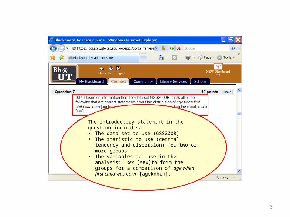
The introductory statement in the question indicates:• The data set to use (GSS200R)• The statistic to use (central tendency and

dispersion) for two or more groups• The variables to use in the analysis: sex [sex]to

form the groups for a comparison of age when first child was born [agekdbrn].

3

The first statement for us to evaluate concerns the number of valid and missing cases. To answer this question, we produce the descriptive statistics using the SPSS Explore procedure.

4

To compute the measures of central tendency and dispersion in SPSS, select the Descriptive Statistics > Explore command from the Analyze menu.

5

Move the variable for the analysis agekdbrn to the Dependent List list box..

Click on the Statistics button to select optional statistics.

6

The check box for Descriptives is already marked by default.

Click on Continue button to close the dialog box.

Mark the Percentiles check box. This will provided the upper and lower bounds for the interquartile range.

7

After returning to the Explore dialog box, click on the OK button to produce the output.

8

The 'Case Processing Summary' in the SPSS output showed the total number of valid cases to be 193 and the number of missing cases to be 77.

The SPSS output provides us with the answer to the question on sample size.

9

The 'Case Processing Summary' in the SPSS output showed the total number of valid cases to be 193 and the number of missing cases to be 77.

Click on the check box to mark the statement as correct.

10

The next pair of statements asks us to identify the direction of the skewing in the distribution of the variable.

11

The skewness for the distribution of "age when first child was born" [agekdbrn] is 1.09. Since this is greater than zero, we characterize it as positive skewing or skewing to the right. If it were less than zero, it would be negative skewing or skewing to the left.

12

The skewness for the distribution of "age when first child was born" [agekdbrn] is 1.09. Since this is greater than zero, we characterize it as positive skewing or skewing to the right.

We mark the check box for the statement with the correct response.

13

The next pair of statements asks us to identify which measure of center and spread should be reported for the variable.

14

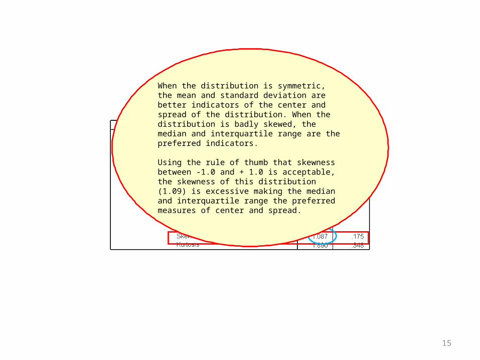
When the distribution is symmetric, the mean and standard deviation are better indicators of the center and spread of the distribution. When the distribution is badly skewed, the median and interquartile range are the preferred indicators.

Using the rule of thumb that skewness between -1.0 and + 1.0 is acceptable, the skewness of this distribution (1.09) is excessive making the median and interquartile range the preferred measures of center and spread.

15

Using the rule of thumb that skewness between -1.0 and + 1.0 is acceptable, the skewness of this distribution (1.09) is excessive making the median and interquartile range the preferred measures of center and spread.

The check box for the second statement is marked.

16

Having decided to use the median and interquartile range to represent the center and spread of the distribution, the next pair of questions ask us to compare the medians of the two groups.

To compare the groups, we need to add the grouping variable to the analysis.

17

Click on the Dialog Recall button on the tool bar.

This button enables us to modify the specifications for previously completed analyses.

18

When we click on the Dialog Recall button, a drop down menu of recently conducted analyses appears.

We click on the Explore menu option to amend the analysis which we just completed.

19

First, move the grouping variable sex to the Factor List list box. Descriptive statistics will be computed for each category of the factor.

Second, click on the OK button to produce the output.

20

Since the distribution of "age when first child was born" [agekdbrn] was badly skewed (1.09), the comparison of the central tendency of the groups is based on the median. ct.

The median for survey respondents who were male (25) is larger than the median for survey respondents who were female (22).

The statement that "survey respondents who were male were older when first child was born than survey respondents who were female" is correct.

21

Since the distribution of "age when first child was born" [agekdbrn] was badly skewed (1.09), the comparison of the central tendency of the groups is based on the median. The median for survey respondents who were male (25) is larger than the median for survey respondents who were female (22).

The statement that "survey respondents who were male were older when first child was born than survey respondents who were female" is correct and is marked.

22

23

The next pair of questions ask us to compare the interquartile ranges of the two groups.

Since the distribution of "age when first child was born" [agekdbrn] was badly skewed (1.09), the comparison of the spread or variability of the groups is based on the interquartile range.

The interquartile range for survey respondents who were male (7) is the same as the interquartile range for survey respondents who were female (7).

Each of the statements about the spread of the distribution imply that one group is more diverse than the other. Since both groups have the same interquartile range, neither statement is correct.

24

Since the distribution of "age when first child was born" [agekdbrn] was badly skewed (1.09), the comparison of the spread or variability of the groups is based on the interquartile range. The interquartile range for survey respondents who were male (7) is the same as the interquartile range for survey respondents who were female (7).

Since both statements imply a difference in the interquartile range, neither is correct and neither one is marked.

25