8 - virtual work
DESCRIPTION
8 - Virtual WorkTRANSCRIPT

Structural Analysis III
Dr. C. Caprani 1
Chapter 8 - Virtual Work
8.1 Introduction ......................................................................................................... 3
8.1.1 General ........................................................................................................... 3
8.1.2 Background .................................................................................................... 4
8.2 The Principle of Virtual Work ......................................................................... 13
8.2.1 Definition ..................................................................................................... 13
8.2.2 Virtual Displacements ................................................................................. 16
8.2.3 Virtual Forces .............................................................................................. 17
8.2.4 Simple Proof using Virtual Displacements ................................................. 18
8.2.5 Internal and External Virtual Work ............................................................. 19
8.3 Application of Virtual Displacements ............................................................. 21
8.3.1 Rigid Bodies ................................................................................................ 21
8.3.2 Deformable Bodies ...................................................................................... 28
8.3.3 Problems ...................................................................................................... 43
8.4 Application of Virtual Forces ........................................................................... 45
8.4.1 Basis ............................................................................................................. 45
8.4.2 Deflection of Trusses ................................................................................... 46
8.4.3 Deflection of Beams and Frames ................................................................ 55
8.4.4 Integration of Bending Moments ................................................................. 62
8.4.5 Problems ...................................................................................................... 74
8.5 Virtual Work for Indeterminate Structures ................................................... 82
8.5.1 General Approach ........................................................................................ 82
8.5.2 Using Virtual Work to Find the Multiplier ................................................. 84

Structural Analysis III
Dr. C. Caprani 2
8.5.3 Indeterminate Trusses .................................................................................. 91
8.5.4 Indeterminate Frames .................................................................................. 95
8.5.5 Multiply-Indeterminate Structures ............................................................ 106
8.5.6 Problems .................................................................................................... 123
8.6 Virtual Work for Self-Stressed Structures ................................................... 132
8.6.1 Background ................................................................................................ 132
8.6.2 Trusses ....................................................................................................... 140
8.6.3 Beams ........................................................................................................ 147
8.6.4 Frames ........................................................................................................ 162
8.6.5 Problems .................................................................................................... 167
8.7 Past Exam Questions ....................................................................................... 170
8.8 References ........................................................................................................ 183
8.9 Appendix – Volume Integrals ......................................................................... 184
Rev. 1

Structural Analysis III
Dr. C. Caprani 3
8.1 Introduction
8.1.1 General
Virtual Work is a fundamental theory in the mechanics of bodies. So fundamental in
fact, that Newton’s 3 equations of equilibrium can be derived from it. Virtual Work
provides a basis upon which vectorial mechanics (i.e. Newton’s laws) can be linked
to the energy methods (i.e. Lagrangian methods) which are the basis for finite
element analysis and advanced mechanics of materials.
Virtual Work allows us to solve determinate and indeterminate structures and to
calculate their deflections. That is, it can achieve everything that all the other
methods together can achieve.
Before starting into Virtual Work there are some background concepts and theories
that need to be covered.

Structural Analysis III
Dr. C. Caprani 4
8.1.2 Background
Strain Energy and Work Done
Strain energy is the amount of energy stored in a structural member due to
deformation caused by an external load. For example, consider this simple spring:
We can see that as it is loaded by a gradually increasing force, F, it elongates. We can
graph this as:
The line OA does not have to be straight, that is, the constitutive law of the spring’s
material does not have to be linear.

Structural Analysis III
Dr. C. Caprani 5
An increase in the force of a small amount, F results in a small increase in
deflection, y . The work done during this movement (force × displacement) is the
average force during the course of the movement, times the displacement undergone.
This is the same as the hatched trapezoidal area above. Thus, the increase in work
associated with this movement is:
2
2
F F FU y
F yF y
F y
(1.1)
where we can neglect second-order quantities. As 0y , we get:
dU F dy
The total work done when a load is gradually applied from 0 up to a force of F is the
summation of all such small increases in work, i.e.:
0
y
U F dy (1.2)
This is the dotted area underneath the load-deflection curve of earlier and represents
the work done during the elongation of the spring. This work (or energy, as they are
the same thing) is stored in the spring and is called strain energy and denoted U.
If the load-displacement curve is that of a linearly-elastic material then F ky where
k is the constant of proportionality (or the spring stiffness). In this case, the dotted
area under the load-deflection curve is a triangle.

Structural Analysis III
Dr. C. Caprani 6
As we know that the work done is the area under this curve, then the work done by
the load in moving through the displacement – the External Work Done, eW - is given
by:
1
2eW Fy (1.3)
We can also calculate the strain energy, or Internal Work Done, IW , by:
0
0
21
2
y
y
U F dy
ky dy
ky
Also, since F ky , we then have:
1 1
2 2IW U ky y Fy

Structural Analysis III
Dr. C. Caprani 7
But this is the external work done, eW . Hence we have:
e IW W (1.4)
Which we may have expected from the Law of Conservation of Energy. Thus:
The external work done by external forces moving through external displacements is
equal to the strain energy stored in the material.

Structural Analysis III
Dr. C. Caprani 8
Law of Conservation of Energy
For structural analysis this can be stated as:
Consider a structural system that is isolated such it neither gives nor receives
energy; the total energy of this system remains constant.
The isolation of the structure is key: we can consider a structure isolated once we
have identified and accounted for all sources of restraint and loading. For example, to
neglect the self-weight of a beam is problematic as the beam receives gravitational
energy not accounted for, possibly leading to collapse.
In the spring and force example, we have accounted for all restraints and loading (for
example we have ignored gravity by having no mass). Thus the total potential energy
of the system, , is constant both before and after the deformation.
In structural analysis the relevant forms of energy are the potential energy of the load
and the strain energy of the material. We usually ignore heat and other energies.
Potential Energy of the Load
Since after the deformation the spring has gained strain energy, the load must have
lost potential energy, V. Hence, after deformation we have for the total potential
energy:
21
2
U V
ky Fy
(1.5)
In which the negative sign indicates a loss of potential energy for the load.

Structural Analysis III
Dr. C. Caprani 9
Principle of Minimum Total Potential Energy
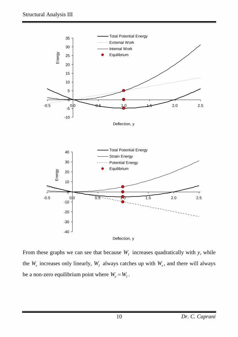
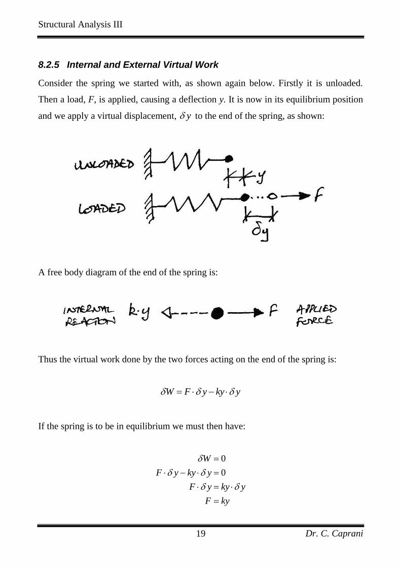
If we plot the total potential energy against y, equation (1.5), we get a quadratic curve
similar to:
Consider a numerical example, with the following parameters, 10 kN/mk and
10 kNF giving the equilibrium deflection as 1 my F k . We can plot the
following quantities:
Internal Strain Energy, or Internal Work: 2 2 21 110 5
2 2IU W ky y y
Potential Energy: 10V Fy y
Total Potential Energy: 25 10U V y y
External Work: 1 1
10 52 2
eW Py y y
and we get the following plots (split into two for clarity):
Structural Analysis III
Dr. C. Caprani 10
From these graphs we can see that because IW increases quadratically with y, while
the eW increases only linearly, IW always catches up with eW , and there will always
be a non-zero equilibrium point where e IW W .
-10
-5
0
5
10
15
20
25
30
35
-0.5 0.0 0.5 1.0 1.5 2.0 2.5
Deflection, y
Energ
y
Total Potential Energy
External Work
Internal Work
Equilibrium
-40
-30
-20
-10
0
10
20
30
40
-0.5 0.0 0.5 1.0 1.5 2.0 2.5
Deflection, y
Energ
y
Total Potential Energy
Strain Energy
Potential Energy
Equilibrium

Structural Analysis III
Dr. C. Caprani 11
Admittedly, these plots are mathematical: the deflection of the spring will not take up
any value; it takes that value which achieves equilibrium. At this point we consider a
small variation in the total potential energy of the system. Considering F and k to be
constant, we can only alter y. The effect of this small variation in y is:
2 2
2
2
1 1
2 2
1 12
2 2
1
2
y y y k y y F y y ky Fy
k y y F y k y
ky F y k y
(1.6)
Similarly to a first derivate, for to be an extreme (either maximum or minimum),
the first variation must vanish:
10ky F y (1.7)
Therefore:
0ky F (1.8)
Which we recognize to be the 0xF . Thus equilibrium occurs when is an
extreme.
Before introducing more complicating maths, an example of the above variation in
equilibrium position is the following. Think of a shopkeeper testing an old type of
scales for balance – she slightly lifts one side, and if it returns to position, and no
large rotations occur, she concludes the scales is in balance. She has imposed a

Structural Analysis III
Dr. C. Caprani 12
variation in displacement, and finds that since no further displacement occurs, the
‘structure’ was originally in equilibrium.
Examining the second variation (similar to a second derivate):
22 10
2k y (1.9)
We can see it is always positive and hence the extreme found was a minimum. This is
a particular proof of the general principle that structures take up deformations that
minimize the total potential energy to achieve equilibrium. In short, nature is lazy!
To summarize our findings:
Every isolated structure has a total potential energy;
Equilibrium occurs when structures can minimise this energy;
A small variation of the total potential energy vanishes when the structure is in
equilibrium.
These concepts are brought together in the Principle of Virtual Work.

Structural Analysis III
Dr. C. Caprani 13
8.2 The Principle of Virtual Work
8.2.1 Definition
Based upon the Principle of Minimum Total Potential Energy, we can see that any
small variation about equilibrium must do no work. Thus, the Principle of Virtual
Work states that:
A body is in equilibrium if, and only if, the virtual work of all forces acting on
the body is zero.
In this context, the word ‘virtual’ means ‘having the effect of, but not the actual form
of, what is specified’. Thus we can imagine ways in which to impose virtual work,
without worrying about how it might be achieved in the physical world.
We need to remind ourselves of equilibrium between internal and external forces, as
well as compatibility of displacement, between internal and external displacements
for a very general structure:
Equilibrium Compatibility

Structural Analysis III
Dr. C. Caprani 14
The Two Principles of Virtual Work
There are two principles that arise from consideration of virtual work, and we use
either as suited to the unknown quantity (force or displacement) of the problem under
analysis.
Principle of Virtual Displacements:
Virtual work is the work done by the actual forces acting on the body moving through
a virtual displacement.
This means we solve an equilibrium problem through geometry, as shown:
(Equilibrium)
Statics
(Compatibility)
Geometry
Principle of Virtual Displacements
External Virtual Work Internal Virtual Work
Real Force (e.g. Point load)
×
Virtual Displacement (e.g. vertical deflection)
Real ‘Force’ (e.g. bending moment)
×
Virtual ‘Displacement’ (e.g. curvature)
equals
Either of these is the
unknown quantity of interest
External compatible
displacements
Virtual Displacements:
Geometry Internal compatible
displacements

Structural Analysis III
Dr. C. Caprani 15
Principle of Virtual Forces:
Virtual work is the work done by a virtual force acting on the body moving through
the actual displacements.
This means we solve a geometry problem through equilibrium as shown below:
(Equilibrium)
Statics
(Compatibility)
Geometry
Principle of Virtual Forces
External Virtual Work Internal Virtual Work
Virtual Force (e.g. Point load)
×
Real Displacement (e.g. vertical deflection)
Virtual ‘Force’ (e.g. bending moment)
×
Real ‘Displacement’ (e.g. curvature)
equals
The unknown quantity of interest
External real
forces
Internal Real ‘Displacements’:
Statics Internal real
‘forces’ Constitutive
relations Internal real
‘displacements’

Structural Analysis III
Dr. C. Caprani 16
8.2.2 Virtual Displacements
A virtual displacement is a displacement that is only imagined to occur. This is
exactly what we did when we considered the vanishing of the first variation of ; we
found equilibrium. Thus the application of a virtual displacement is a means to find
this first variation of .
So given any real force, F, acting on a body to which we apply a virtual
displacement. If the virtual displacement at the location of and in the direction of F is
y , then the force F does virtual work W F y .
There are requirements on what is permissible as a virtual displacement. For
example, in the simple proof of the Principle of Virtual Work (to follow) it can be
seen that it is assumed that the directions of the forces applied to P remain
unchanged. Thus:
virtual displacements must be small enough such that the force directions are
maintained.
The other very important requirement is that of compatibility:
virtual displacements within a body must be geometrically compatible with
the original structure. That is, geometrical constraints (i.e. supports) and
member continuity must be maintained.
In summary, virtual displacements are not real, they can be physically impossible but
they must be compatible with the geometry of the original structure and they must be
small enough so that the original geometry is not significantly altered.
As the deflections usually encountered in structures do not change the overall
geometry of the structure, this requirement does not cause problems.

Structural Analysis III
Dr. C. Caprani 17
8.2.3 Virtual Forces
So far we have only considered small virtual displacements and real forces. The
virtual displacements are arbitrary: they have no relation to the forces in the system,
or its actual deformations. Therefore virtual work applies to any set of forces in
equilibrium and to any set of compatible displacements and we are not restricted to
considering only real force systems and virtual displacements. Hence, we can use a
virtual force system and real displacements. Obviously, in structural design it is these
real displacements that are of interest and so virtual forces are used often.
A virtual force is a force imagined to be applied and is then moved through the actual
deformations of the body, thus causing virtual work.
So if at a particular location of a structure, we have a deflection, y, and impose a
virtual force at the same location and in the same direction of F we then have the
virtual work W y F .
Virtual forces must form an equilibrium set of their own. For example, if a virtual
force is applied to the end of a spring there will be virtual stresses in the spring as
well as a virtual reaction.

Structural Analysis III
Dr. C. Caprani 18
8.2.4 Simple Proof using Virtual Displacements
We can prove the Principle of Virtual Work quite simply, as follows. Consider a
particle P under the influence of a number of forces 1, , nF F which have a resultant
force, RF . Apply a virtual displacement of y to P, moving it to P’, as shown:
The virtual work done by each of the forces is:
1 1 n n R RW F y F y F y
Where 1y is the virtual displacement along the line of action of 1F and so on. Now
if the particle P is in equilibrium, then the forces 1, , nF F have no resultant. That is,
there is no net force. Hence we have:
1 10 0R n nW y F y F y (2.1)
Proving that when a particle is in equilibrium the virtual work of all the forces acting
on it sum to zero. Conversely, a particle is only in equilibrium if the virtual work
done during a virtual displacement is zero.
Structural Analysis III
Dr. C. Caprani 19
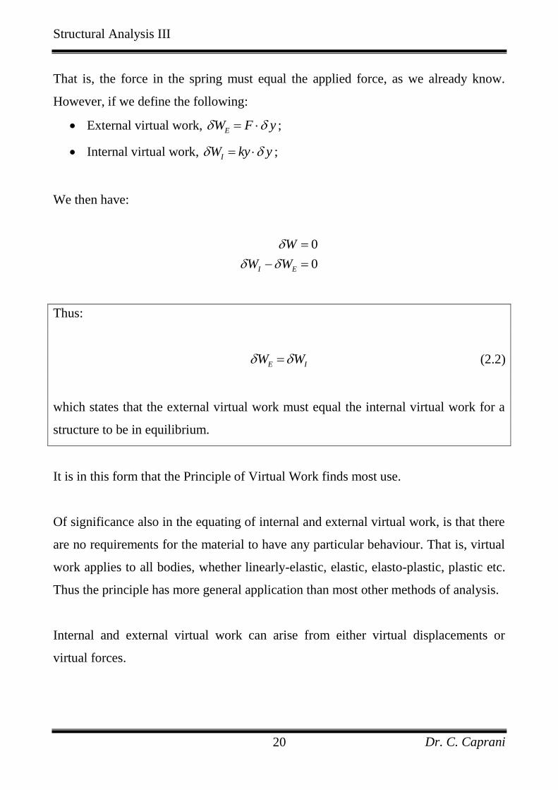
8.2.5 Internal and External Virtual Work
Consider the spring we started with, as shown again below. Firstly it is unloaded.
Then a load, F, is applied, causing a deflection y. It is now in its equilibrium position
and we apply a virtual displacement, y to the end of the spring, as shown:
A free body diagram of the end of the spring is:
Thus the virtual work done by the two forces acting on the end of the spring is:
W F y ky y
If the spring is to be in equilibrium we must then have:
0
0
W
F y ky y
F y ky y
F ky
Structural Analysis III
Dr. C. Caprani 20
That is, the force in the spring must equal the applied force, as we already know.
However, if we define the following:
External virtual work, EW F y ;
Internal virtual work, IW ky y ;
We then have:
0
0I E
W
W W
Thus:
E IW W (2.2)
which states that the external virtual work must equal the internal virtual work for a
structure to be in equilibrium.
It is in this form that the Principle of Virtual Work finds most use.
Of significance also in the equating of internal and external virtual work, is that there
are no requirements for the material to have any particular behaviour. That is, virtual
work applies to all bodies, whether linearly-elastic, elastic, elasto-plastic, plastic etc.
Thus the principle has more general application than most other methods of analysis.
Internal and external virtual work can arise from either virtual displacements or
virtual forces.

Structural Analysis III
Dr. C. Caprani 21
8.3 Application of Virtual Displacements
8.3.1 Rigid Bodies
Basis
Rigid bodies do not deform and so there is no internal virtual work done. Thus:
0
0
E I
i i
W
W W
F y
(3.1)
A simple application is to find the reactions of statically determinate structures.
However, to do so, we need to make use of the following principle:
Principle of Substitution of Constraints
Having to keep the constraints in place is a limitation of virtual work. However, we
can substitute the restraining force (i.e. the reaction) in place of the restraint itself.
That is, we are turning a geometric constraint into a force constraint. This is the
Principle of Substitution of Constraints. We can use this principle to calculate
unknown reactions:
1. Replace the reaction with its appropriate force in the same direction (or sense);
2. Impose a virtual displacement on the structure;
3. Calculate the reaction, knowing 0W .

Structural Analysis III
Dr. C. Caprani 22
Reactions of Determinate and Indeterminate Structures
For statically determinate structures, removing a restraint will always render a
mechanism (or rigid body) and so the reactions of statically determinate structures are
easily obtained using virtual work. For indeterminate structures, removing a restraint
does not leave a mechanism and hence the virtual displacements are harder to
establish since the body is not rigid.

Structural Analysis III
Dr. C. Caprani 23
Example 1
Problem
Determine the reactions for the following beam:
Solution
Following the Principle of Substitution of Constraints, we replace the geometric
constraints (i.e. supports), by their force counterparts (i.e. reactions) to get the free-
body-diagram of the whole beam:
Next, we impose a virtual displacement on the beam. Note that the displacement is
completely arbitrary, and the beam remains rigid throughout:

Structural Analysis III
Dr. C. Caprani 24
In the above figure, we have imposed a virtual displacement of Ay at A and then
imposed a virtual rotation of A about A. The equation of virtual work is:
0
0
E I
i i
W
W W
F y
Hence:
0A A C B BV y P y V y
Relating the virtual movements of points B and C to the virtual displacements gives:
0A A A A B A AV y P y a V y L
And rearranging gives:
0A B A B AV V P y V L Pa

Structural Analysis III
Dr. C. Caprani 25
And here is the power of virtual work: since we are free to choose any value we want
for the virtual displacements (i.e. they are completely arbitrary), we can choose
0A and 0Ay , which gives the following two equations:
0
0
A B A
A B
V V P y
V V P
0
0
B A
B
V L Pa
V L Pa
But the first equation is just 0yF whilst the second is the same as
about 0M A . Thus equilibrium equations occur naturally within the virtual
work framework. Note also that the two choices made for the virtual displacements
correspond to the following virtual displaced configurations:

Structural Analysis III
Dr. C. Caprani 26
Example 2
Problem
For the following truss, calculate the reaction CV :
Solution
Firstly, set up the free-body-diagram of the whole truss:
Structural Analysis III
Dr. C. Caprani 27
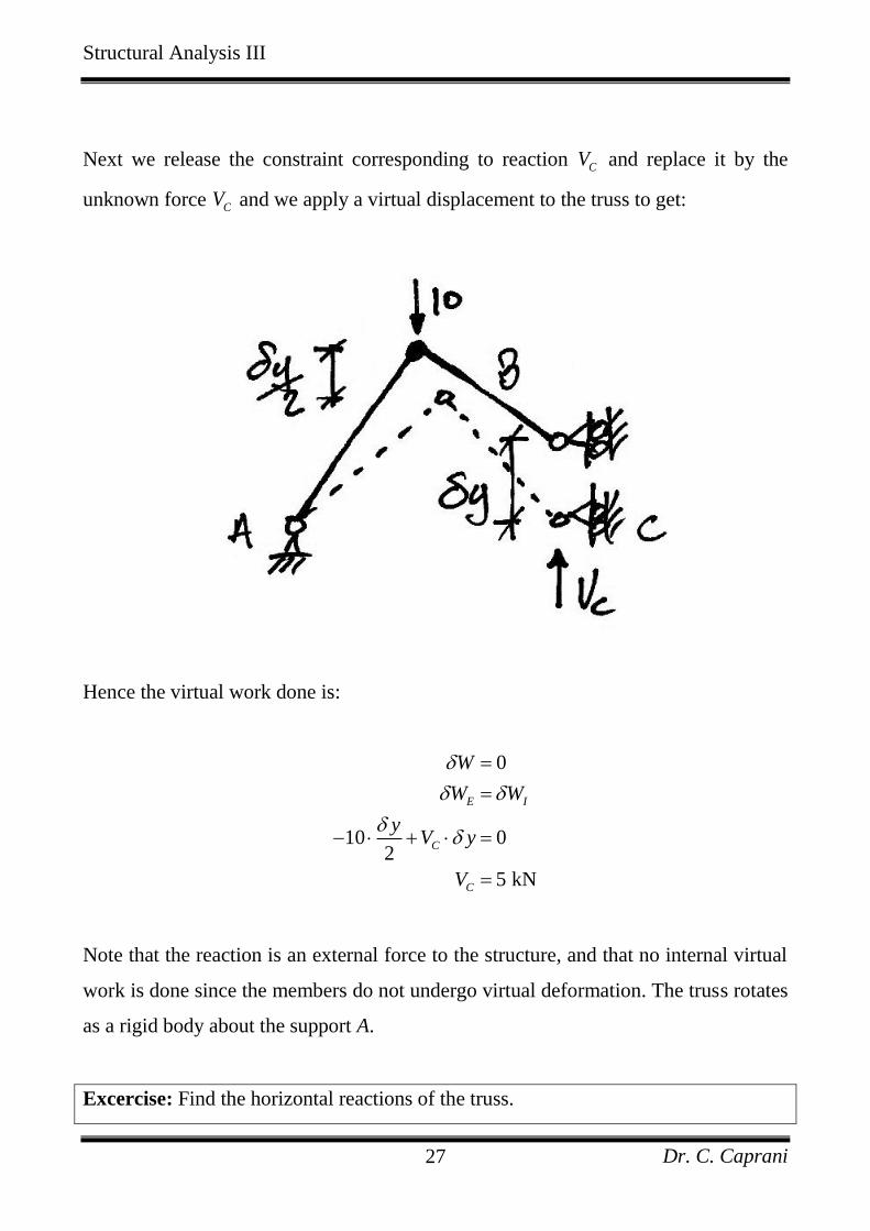
Next we release the constraint corresponding to reaction CV and replace it by the
unknown force CV and we apply a virtual displacement to the truss to get:
Hence the virtual work done is:
0
10 02
5 kN
E I
C
C
W
W W
yV y
V
Note that the reaction is an external force to the structure, and that no internal virtual
work is done since the members do not undergo virtual deformation. The truss rotates
as a rigid body about the support A.
Excercise: Find the horizontal reactions of the truss.
Structural Analysis III
Dr. C. Caprani 28
8.3.2 Deformable Bodies
Basis
For a virtual displacement we have:
0
E I
i i i i
W
W W
F y P e
For the external virtual work, iF represents an externally applied force (or moment)
and iy is its corresponding virtual displacement. For the internal virtual work, iP is
the internal force in member i and ie is its virtual deformation. Different stress
resultants have different forms of internal work, and we will examine these. The
summations reflect the fact that all work done must be accounted for. Remember in
the above, each the displacements must be compatible and the forces must be in
equilibrium, summarized as:
These displacements are completely arbitrary (i.e. we can choose them to suit our
purpose) and bear no relation to the forces above.
Set of forces in
equilibrium
Set of compatible
displacements

Structural Analysis III
Dr. C. Caprani 29
Example 3
Problem
For the simple truss, show the forces are as shown using the principle of virtual
displacements.
Loading and dimensions Equilibrium forces and actual deformation
Solution
An arbitrary set of permissible compatible displacements are shown:
Compatible set of displacements

Structural Analysis III
Dr. C. Caprani 30
To solve the problem though, we need to be thoughtful about the choice of arbitrary
displacement: we only want the unknown we are currently calculating to do work,
otherwise there will be multiple unknowns in the equation of virtual work. Consider
this possible compatible set of displacements:
Assuming both forces are tensile, and noting that the load does no work since the
virtual external displacement is not along its line of action, the virtual work done is:
1 1 2 2
0
40 0
E I
W
W W
e F e F
Since the displacements are small and compatible, we know by geometry that:
1 2
3
5y e e

Structural Analysis III
Dr. C. Caprani 31
Giving:
1 2
1 2
30
5
3
5
y F y F
F F
which tells us that one force is in tension and the other in compression.
Unfortunately, this displaced configuration was not sufficient as we were left with
two unknowns. Consider the following one though:
2 2
0
40
E I
W
W W
y e F
The negative signs appear because the 40 kN load moves against its direction, and the
(assumed) tension member AB is made shorter which is against its ‘tendency’ to
elongate. Also, by geometry:
2
4
5y e

Structural Analysis III
Dr. C. Caprani 32
And so:
2
2
440
5
50 kN
y y F
F
The positive result indicates that the member is in tension as was assumed. Now we
can return to the previous equation to get:
1
350 30 kN
5F
And so the member is in compression, since the negative tells us that it is in the
opposite direction to that assumed, which was tension.
Structural Analysis III
Dr. C. Caprani 33
Internal Virtual Work by Axial Force
Members subject to axial force may have the following:
real force by a virtual displacement:
IW P e
virtual force by a real displacement:
IW e P
We have avoided integrals over the length of the member since we will only consider
prismatic members.

Structural Analysis III
Dr. C. Caprani 34
Internal Virtual Work in Bending
The internal virtual work done in bending is one of:
real moment by a virtual curvature:
IW M
virtual moment by a real curvature:
IW M
The above expressions are valid at a single position in a beam.
When virtual rotations are required along the length of the beam, the easiest way to
do this is by applying virtual loads that in turn cause virtual moments and hence
virtual curvatures. We must sum all of the real moments by virtual curvatures along
the length of the beam, hence we have:
0 0
0
L L
I x x x x
L
xx
x
W M dx M dx
MM dx
EI
Structural Analysis III
Dr. C. Caprani 35
Internal Virtual Work in Shear
At a single point in a beam, the shear strain, , is given by:
v
V
GA
where V is the applied shear force, G is the shear modulus and vA is the cross-section
area effective in shear which is explained below. The internal virtual work done in
shear is thus:
real shear force by a virtual shear strain:
I
v
VW V V
GA
virtual shear force by a real shear strain:
I
v
VW V V
GA
These expressions are valid at a single position in a beam and must be integrated
along the length of the member as was done for moments and rotations.
The area of cross section effective in shear arises because the shear stress (and hence
strain) is not constant over a cross section. The stress vV A is an average stress,
equivalent in work terms to the actual uneven stress over the full cross section, A. We
say vA A k where k is the shear factor. Some values of k are: 1.2 for rectangular
sections; 1.1 for circular sections; and 2.0 for thin-walled circular sections.

Structural Analysis III
Dr. C. Caprani 36
Internal Virtual Work in Torsion
At a single point in a member, the twist, , is given by:
T
GJ
where T is the applied torque, G is the shear modulus, J is the polar moment of
inertia. The internal virtual work done in torsion is thus:
real torque by a virtual twist:
I
TW T T
GJ
virtual torque by a real twist:
I
TW T T
GJ
Once again, the above expressions are valid at a single position in a beam and must
be integrated along the length of the member as was done for moments and rotations.
Note the similarity between the expressions for the four internal virtual works.

Structural Analysis III
Dr. C. Caprani 37
Example 4
Problem
For the beam of Example 1 (shown again), find the bending moment at C.
Solution
To solve this, we want to impose a virtual displacement configuration that only
allows the unknown of interest, i.e. CM , to do any work. Thus choose the following:
Since portions AC and CB remain straight (or unbent) no internal virtual work is done
in these sections. Thus the only internal work is done at C by the beam moving
through the rotation at C. Thus:

Structural Analysis III
Dr. C. Caprani 38
0
E I
C C C
W
W W
P y M
Bu the rotation at C is made up as:
C CA CB
C C
C
y y
a b
a by
ab
But a b L , hence:
C C C
C
LP y M y
ab
PabM
L
We can verify this from the reactions found previously: C BM V b Pa L b .
Structural Analysis III
Dr. C. Caprani 39
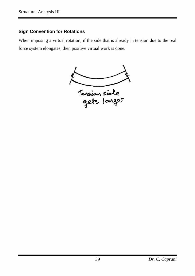
Sign Convention for Rotations
When imposing a virtual rotation, if the side that is already in tension due to the real
force system elongates, then positive virtual work is done.

Structural Analysis III
Dr. C. Caprani 40
Virtual Work done by Distributed Load
The virtual work done by an arbitrary distributed load moving through a virtual
displacement field is got by summing the infinitesimal components:
2
1
x
e
x
W y x w x dx
Considering the special (but very common) case of a uniformly distributed load:
2
1
Area of diagram
x
e
x
W w y x dx w y
If we denote the length of the load as 2 1L x x then we can say that the area of the
displacement diagram is the average displacement, y , times the length, L. Thus:
Total load Average displacementeW wL y
Structural Analysis III
Dr. C. Caprani 41
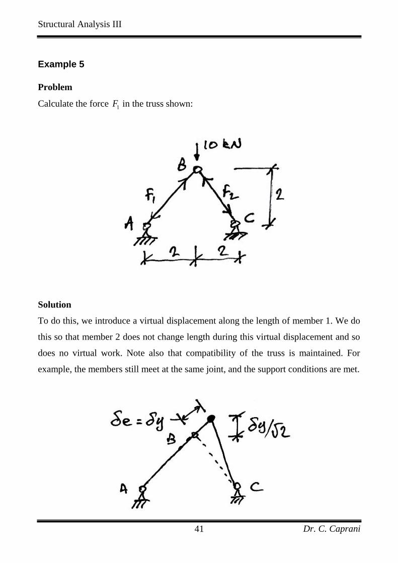
Example 5
Problem
Calculate the force 1F in the truss shown:
Solution
To do this, we introduce a virtual displacement along the length of member 1. We do
this so that member 2 does not change length during this virtual displacement and so
does no virtual work. Note also that compatibility of the truss is maintained. For
example, the members still meet at the same joint, and the support conditions are met.

Structural Analysis III
Dr. C. Caprani 42
The virtual work done is then:
1
1
0
102
105 2 kN
2
E I
W
W W
yF y
F
Note some points on the signs used:
1. Negative external work is done because the 10 kN load moves upwards; i.e. the
reverse direction to its action.
2. We assumed member 1 to be in compression but then applied a virtual
elongation which lengthened the member thus reducing its internal virtual
work. Hence negative internal work is done.
3. We initially assumed 1F to be in compression and we obtained a positive
answer confirming our assumption.
Exercise: Investigate the vertical and horizontal equilibrium of the loaded joint by
considering vertical and horizontal virtual displacements separately.

Structural Analysis III
Dr. C. Caprani 43
8.3.3 Problems
1. For the truss shown, calculate the vertical reaction at C and the forces in the
members, using virtual work.
2. For the truss shown, find the forces in the members, using virtual work:
Structural Analysis III
Dr. C. Caprani 44
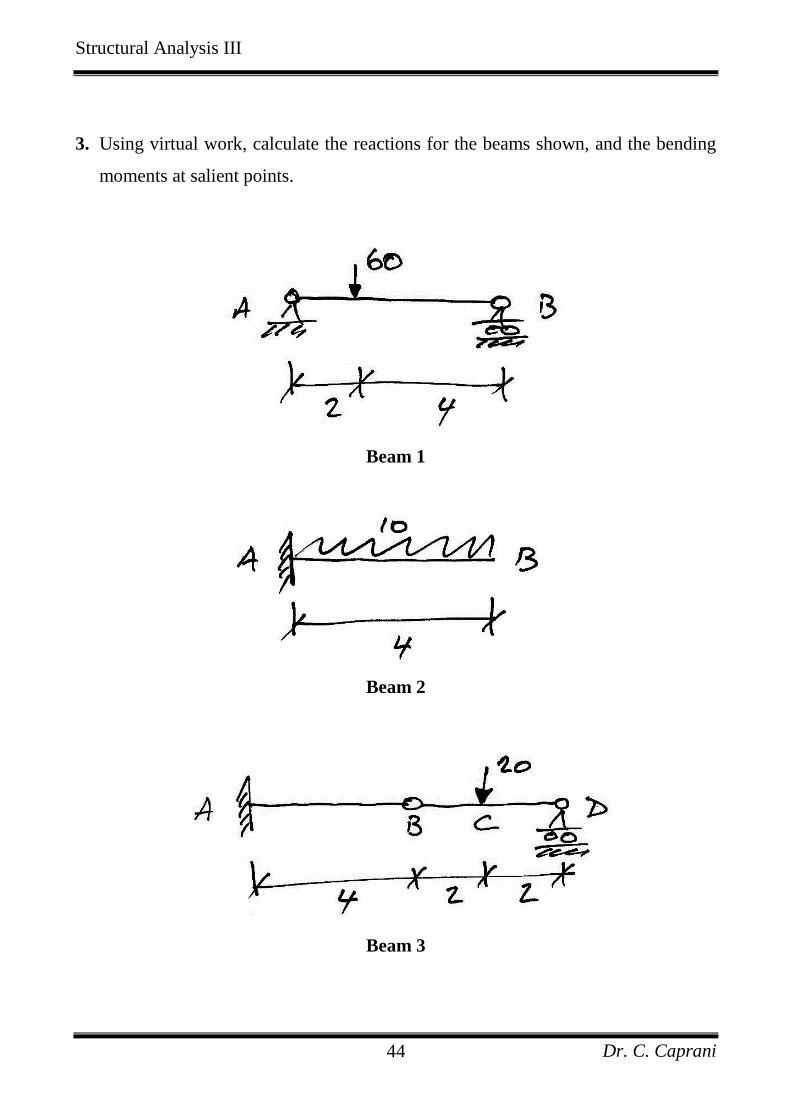
3. Using virtual work, calculate the reactions for the beams shown, and the bending
moments at salient points.
Beam 1
Beam 2
Beam 3
Structural Analysis III
Dr. C. Caprani 45
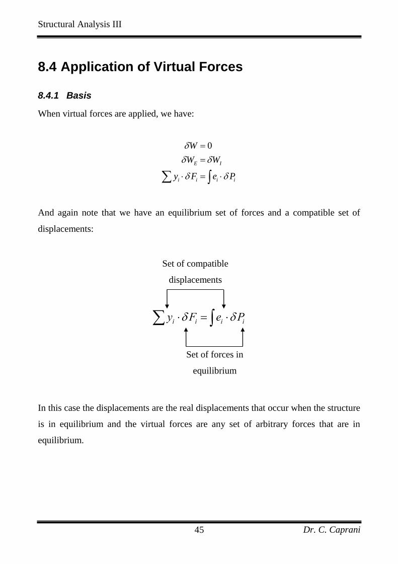
8.4 Application of Virtual Forces
8.4.1 Basis
When virtual forces are applied, we have:
0
E I
i i i i
W
W W
y F e P
And again note that we have an equilibrium set of forces and a compatible set of
displacements:
In this case the displacements are the real displacements that occur when the structure
is in equilibrium and the virtual forces are any set of arbitrary forces that are in
equilibrium.
Set of compatible
displacements
Set of forces in
equilibrium

Structural Analysis III
Dr. C. Caprani 46
8.4.2 Deflection of Trusses
Basis
In a truss, we know:
1. The forces in the members (got from virtual displacements or statics);
2. Hence we can calculate the member extensions, ie as:
i
i
PLe
EA
3. The virtual work equation is:
0
E I
i i i i
W
W W
y F e P
4. To find the deflection at a single joint on the truss we apply a unit virtual force at
that joint, in the direction of the required displacement, giving:
i
i
PLy P
EA
5. Since in this equation, y is the only unknown, we can calculate the deflection of
the truss at the joint being considered.
Structural Analysis III
Dr. C. Caprani 47
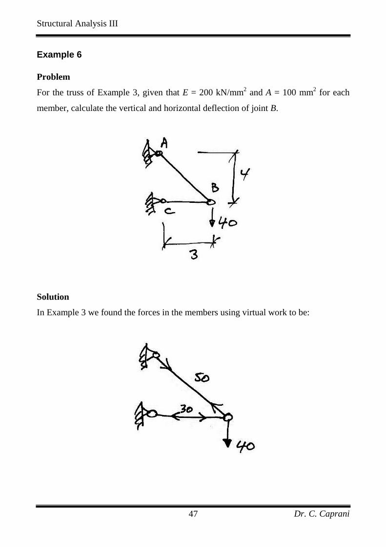
Example 6
Problem
For the truss of Example 3, given that E = 200 kN/mm2 and A = 100 mm
2 for each
member, calculate the vertical and horizontal deflection of joint B.
Solution
In Example 3 we found the forces in the members using virtual work to be:

Structural Analysis III
Dr. C. Caprani 48
The actual (real) compatible displacements are shown:
Two possible sets of virtual forces are:
In these problems we will always choose 1F . Hence we apply a unit virtual force
to joint B. We apply the force in the direction of the deflection required. In this way
no work is done along deflections that are not required. Hence we have:

Structural Analysis III
Dr. C. Caprani 49
For horizontal deflection For vertical deflection
The forces and elongations of the truss members are:
Member AB:
50 kN
50 5000
200 100
12.5 mm
AB
AB
P
e
Member BC:
30 kN
30 3000
200 100
4.5 mm
BC
BC
P
e
Note that by taking tension to be positive, elongations are positive and contractions
are negative.

Structural Analysis III
Dr. C. Caprani 50
Horizontal Deflection:
0
1 12.5 0 4.5 1
4.5 mm
E I
i i i i
AB BC
W
W W
y F e P
y
y
Vertical Deflection:
5 31 12.5 4.5
4 4
18.4 mm
i i i i
AB BC
y F e P
y
y
Note that the sign of the result indicates whether the deflection occurs in the same
direction as the applied force. Hence, joint B moves 4.5 mm to the left.

Structural Analysis III
Dr. C. Caprani 51
Example 7
Problem
Determine the vertical and horizontal deflection of joint D of the truss shown. Take E
= 200 kN/mm2 and member areas, A = 1000 mm
2 for all members except AE and BD
where A = 10002 mm2.
Solution
The elements of the virtual work equation are:
Compatible deformations: The actual displacements that the truss undergoes;
Equilibrium set: The external virtual force applied at the location of the required
deflection and the resulting internal member virtual forces.
Firstly we analyse the truss to determine the member forces in order to calculate the
actual deformations of each member:

Structural Analysis III
Dr. C. Caprani 52
Next, we apply a unit virtual force in the vertical direction at joint D. However, by
linear superposition, we know that the internal forces due to a unit load will be 1/150
times those of the 150 kN load.
For the horizontal deflection at D, we apply a unit horizontal virtual force as shown:
Equations of Virtual Work
01
02
0
1
1
E I
i i i i
DV i
i
DH i
i
W
W W
y F e P
P Ly P
EA
P Ly P
EA
In which:

Structural Analysis III
Dr. C. Caprani 53
0P are the forces due to the 150 kN load;
1P are the virtual forces due to the unit virtual force applied in the vertical
direction at D:
0
1
150
PP
2P are the virtual forces due to the unit virtual force in the horizontal
direction at D.
Using a table is easiest because of the larger number of members:
Member L A 0P
01
150
PP 2P
01P L
PA
0
2P LP
A
(mm) (mm2) (kN) (kN) (kN) (kN/mm)×kN (kN/mm)×kN
AB
AE
AF
BC
BD
BE
CD
DE
EF
2000
2000√2
2000
2000
2000√2
2000
2000
2000
2000
1000
1000√2
1000
1000
1000√2
1000
1000
1000
1000
+150
+150√2
0
0
+150√2
-150
0
-150
-300
+1
+1√2
0
0
+1√2
-1
0
-1
-2
0
0
0
0
0
0
0
+1
+1
+300
+600
0
0
+600
+300
0
+300
+1200
0
0
0
0
0
0
0
-300
-600
3300 -900
E is left out because it is common. Returning to the equations, we now have:

Structural Analysis III
Dr. C. Caprani 54
011
1
330016.5 mm
200
DV i
i
DV
P Ly P
E A
y
Which indicates a downwards deflection and for the horizontal deflection:
021
1
9004.5 mm
200
DH i
i
DH
P Ly P
E A
y
The sign indicates that it is deflecting to the left.

Structural Analysis III
Dr. C. Caprani 55
8.4.3 Deflection of Beams and Frames
Example 8
Problem
Using virtual work, calculate the deflection at the centre of the beam shown, given
that EI is constant.
Solution
To calculate the deflection at C, we will be using virtual forces. Therefore the two
relevant sets are:
Compatibility set: the actual deflection at C and the rotations that occur along
the length of the beam;
Equilibrium set: a unit virtual force applied at C which is in equilibrium with
the internal virtual moments it causes.
Compatibility Set:
The external deflection at C is what is of interest to us. To calculate the rotations
along the length of the beam we have:
xx
x
M
EI

Structural Analysis III
Dr. C. Caprani 56
Hence we need to establish the bending moments along the beam:
For AC the bending moment is given by (and similarly for B to C):
2
x
PM x
Equilibrium Set:
As we choose the value for 1F , we are only left to calculate the virtual moments:
For AC the internal virtual moments are given by:

Structural Analysis III
Dr. C. Caprani 57
1
2xM x
Virtual Work Equation
0
E I
i i i i
W
W W
y F M
Substitute in the values we have for the real rotations and the virtual moments, and
use the fact that the bending moment diagrams are symmetrical:
2
0
2
0
2
2
0
23
0
3
3
1 2
2 1
2 2
2
4
2 3
6 8
48
L
xx
L
L
L
My M dx
EI
Py x x dx
EI
Px dx
EI
P x
EI
P L
EI
PL
EI
Which is a result we expected.

Structural Analysis III
Dr. C. Caprani 58
Example 9
Problem
Find the vertical and horizontal displacement of the prismatic curved bar shown:
Solution
Even though it is curved, from the statics, the bending moment at any point of course
remains force by distance, so from the following diagram:

Structural Analysis III
Dr. C. Caprani 59
At any angle , we therefore have:
cos
1 cos
M P R R
PR
To find the displacements, we follow our usual procedure and place a unit load at the
location of, and in the direction of, the required displacement.
Vertical Displacement
The virtual bending moment induced by the vertical unit load shown, is related to that
for P and is thus:
1 cosM R
Thus our virtual work equations are:
Structural Analysis III
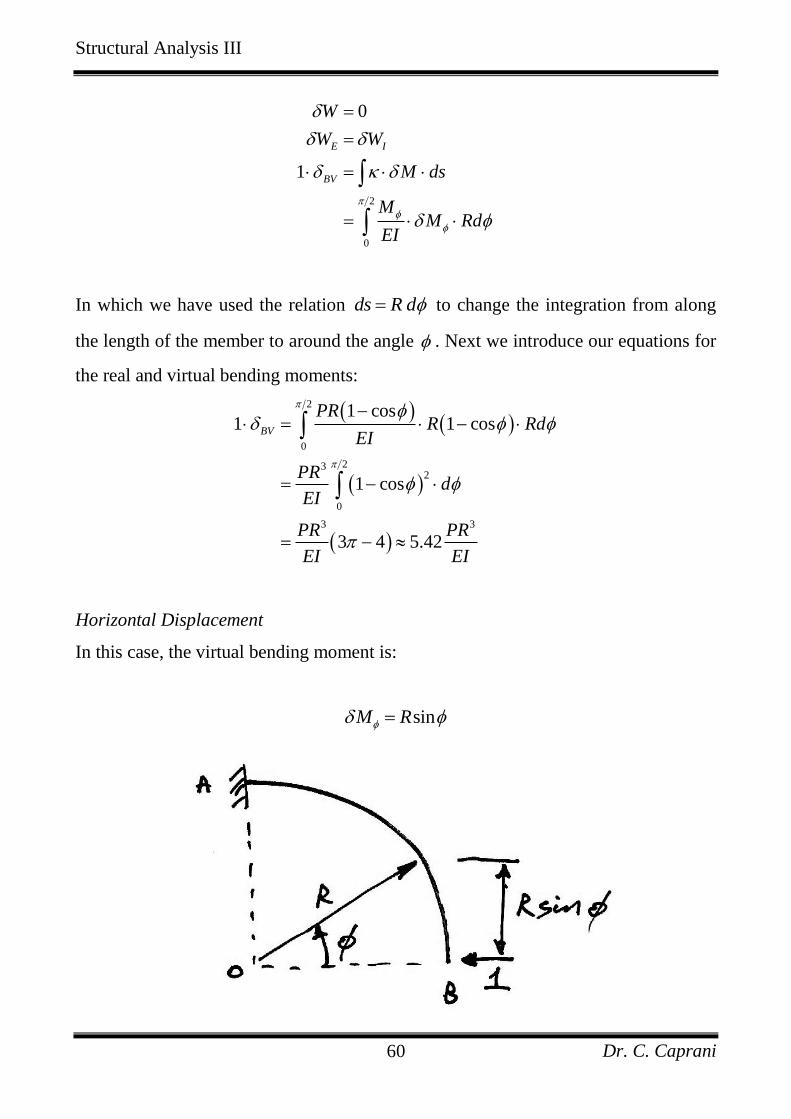
Dr. C. Caprani 60
2
0
0
1
E I
BV
W
W W
M ds
MM Rd
EI
In which we have used the relation ds R d to change the integration from along
the length of the member to around the angle . Next we introduce our equations for
the real and virtual bending moments:
2
0
232
0
3 3
1 cos1 1 cos
1 cos
3 4 5.42
BV
PRR Rd
EI
PRd
EI
PR PR
EI EI
Horizontal Displacement
In this case, the virtual bending moment is:
sinM R

Structural Analysis III
Dr. C. Caprani 61
Thus the virtual work equations give:
2
0
23
0
23
0
3 3
1 cos1 sin
sin sin cos
sin 2sin
2
1
2 2
BH
PRR Rd
EI
PRd
EI
PRd
EI
PR PR
EI EI

Structural Analysis III
Dr. C. Caprani 62
8.4.4 Integration of Bending Moments
General Volume Integral Expression
We are often faced with the integration of being moment diagrams when using virtual
work to calculate the deflections of bending members. And as bending moment
diagrams only have a limited number of shapes, a table of ‘volume’ integrals is used:
Derivation
The general equation for the volume integral is derived consider the real bending
moment diagram as parabolic, and the virtual bending moment diagram as linear:
In terms of the left and right end (y0 and yL respectively) and midpoint value (ym), a
second degree parabola can be expressed as:
2
0 0 02 2 4 3L m m L
x xy x y y y y y y y
L L
Structural Analysis III
Dr. C. Caprani 63
For the case linear case, 00.5m Ly y y , and the expression reduces to that of
straight line. For the real bending moment (linear or parabolic) diagram, we therefore
have:
2
0 0 02 2 4 3L m m L
x xM x M M M M M M M
L L
And for the linear virtual moment diagram we have:
0 0L
xM x M M M
L
The volume integral is given by:
0
L
V M M dx
Which using Simpsons Rule, reduces to:
0 0
0
46
L
m m L L
LM M dx M M M M M M
This expression is valid for the integration of all linear by linear or parabolic
diagrams.
Structural Analysis III
Dr. C. Caprani 64
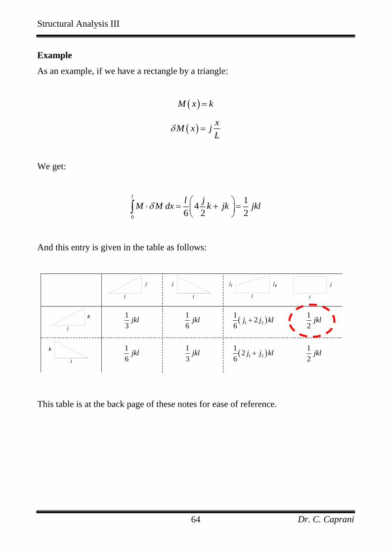
Example
As an example, if we have a rectangle by a triangle:
M x k
x
M x jL
We get:
0
14
6 2 2
ll j
M M dx k jk jkl
And this entry is given in the table as follows:
This table is at the back page of these notes for ease of reference.
1
3jkl
1
6jkl 1 2
12
6j j kl
1
2jkl
1
6jkl
1
3jkl 1 2
12
6j j kl
1
2jkl
1 2
1 2
1 2
1 2
1 2
1 2
1 2
1 2
1 2
1 2
1 2
1 2
Structural Analysis III
Dr. C. Caprani 65
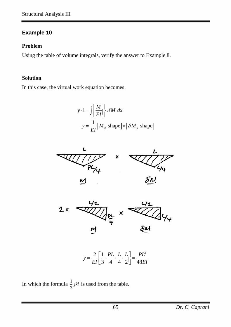
Example 10
Problem
Using the table of volume integrals, verify the answer to Example 8.
Solution
In this case, the virtual work equation becomes:
1
1 shape shapex x
My M dx
EI
y M MEI
32 1
3 4 4 2 48
PL L L PLy
EI EI
In which the formula 1
3jkl is used from the table.

Structural Analysis III
Dr. C. Caprani 66
Example 11
Problem
Determine the influence of shear deformation on the deflection of a rectangular
prismatic mild steel cantilever subjected to point load at its tip.
Solution
Since we are calculating deflections, and must include the shear contribution, we
apply a virtual unit point load at the tip and determine the real and virtual bending
moment and shear force diagrams:
The virtual work done has contributions by both the bending and shear terms:
0
1
E I
v
W
W W
M ds V ds
M VM ds V ds
EI GA
Structural Analysis III
Dr. C. Caprani 67
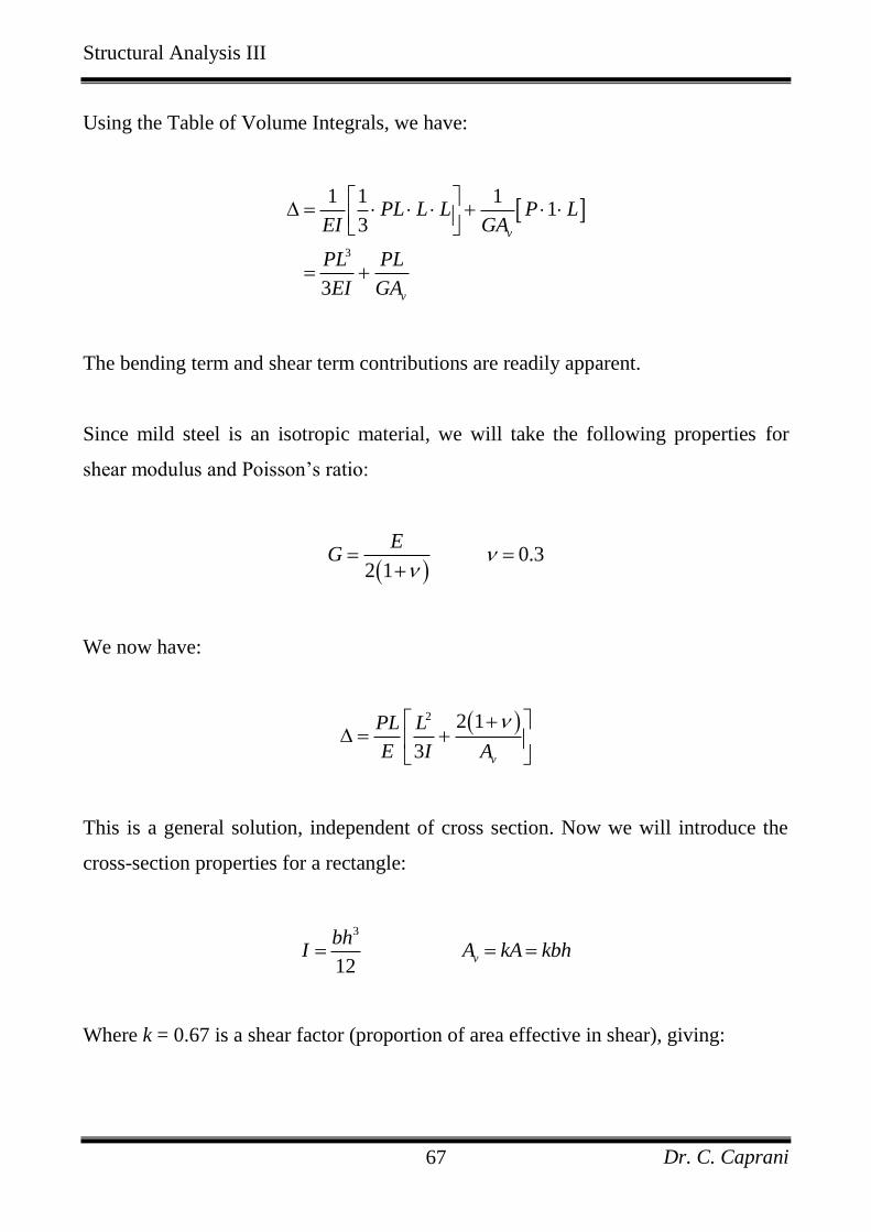
Using the Table of Volume Integrals, we have:
3
1 1 11
3
3
v
v
PL L L P LEI GA
PL PL
EI GA
The bending term and shear term contributions are readily apparent.
Since mild steel is an isotropic material, we will take the following properties for
shear modulus and Poisson’s ratio:
0.32 1
EG
We now have:
2 2 1
3 v
PL L
E I A
This is a general solution, independent of cross section. Now we will introduce the
cross-section properties for a rectangle:
3
12v
bhI A kA kbh
Where k = 0.67 is a shear factor (proportion of area effective in shear), giving:
Structural Analysis III
Dr. C. Caprani 68
2
3
2
2 112
3
2 14
PL L
E bh kbh
PL L
Ebh h k
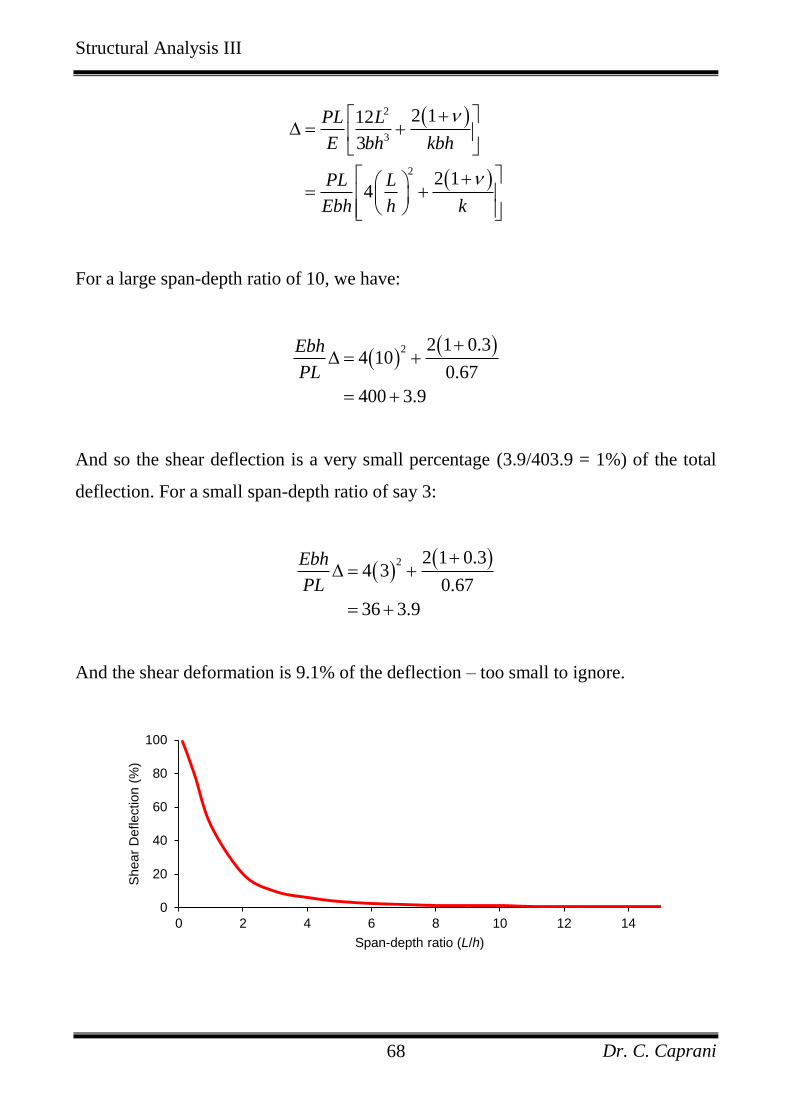
For a large span-depth ratio of 10, we have:
2 2 1 0.34 10
0.67
400 3.9
Ebh
PL
And so the shear deflection is a very small percentage (3.9/403.9 = 1%) of the total
deflection. For a small span-depth ratio of say 3:
2 2 1 0.34 3
0.67
36 3.9
Ebh
PL
And the shear deformation is 9.1% of the deflection – too small to ignore.
0
20
40
60
80
100
0 2 4 6 8 10 12 14
Shear
Deflection (
%)
Span-depth ratio (L/h)

Structural Analysis III
Dr. C. Caprani 69
Example 12
Problem
Determine the static deflection a vehicle experiences as it crosses a simply-supported
bridge. Model the vehicle as a point load.
Solution
Since the vehicle moves across the bridge we need to calculate its deflection at some
arbitrary location along the bridge. Let’s say that at some point in time it is at a
fraction along the length of the bridge:
To determine the deflection at C at this point in time, we apply a unit virtual force at
C. Thus, we have both real and virtual bending moment diagrams:

Structural Analysis III
Dr. C. Caprani 70
The equation for the real bending moment at C is:
1
1C
P L LM PL
L
And similarly:
1CdM L
Thus:
0
1
11 1
3
11 1 1
3
E I
C
AC
CB
W
W W
M ds
MM ds
EI
L L LP
EIL L L
Which after some algebra gives the rather delightful:
3
2
13
C
PL
EI
For 0.5 this reduces to the familiar:

Structural Analysis III
Dr. C. Caprani 71
3 3
2
0.5 1 0.53 48
C
PL PL
EI EI
If the vehicle is travelling at a constant speed v, then its position at time t is x = vt.
Hence is fraction along the length of the bridge is:
x vt
L L
The proportion of deflection related to the midspan deflection is thus:
32
2
3
0.5
1483 13
48
PL
EIPL
EI
And so:
2
0.5
481
3
0
20
40
60
80
100
0 0.2 0.4 0.6 0.8 1
De
fle
ctio
n (
%)
Location along beam (x/L)

Structural Analysis III
Dr. C. Caprani 72
Example 13 – Summer ’07 Part (a)
Problem
For the frame shown, determine the horizontal deflection of joint C. Neglect axial
effects in the members and take 3 236 10 kNmEI .
Solution
Firstly we establish the real bending moment diagram:
FIG. Q3(a)

Structural Analysis III
Dr. C. Caprani 73
Next, as usual, we place a unit load at the location of, and in the direction of, the
required displacement:
Now we have the following for the virtual work equation:
0
1
E I
CH
W
W W
M ds
MM ds
EI
Next, using the table of volume integrals, we have:
1 1 1
440 2 4 2 2 160 2 440 43 6
1659.3 1386.7 3046
AB BC
MM ds
EI EI
EI EI EI
Hence:
3
3
3046 30461 10 84.6 mm
36 10CH
EI
Structural Analysis III
Dr. C. Caprani 74
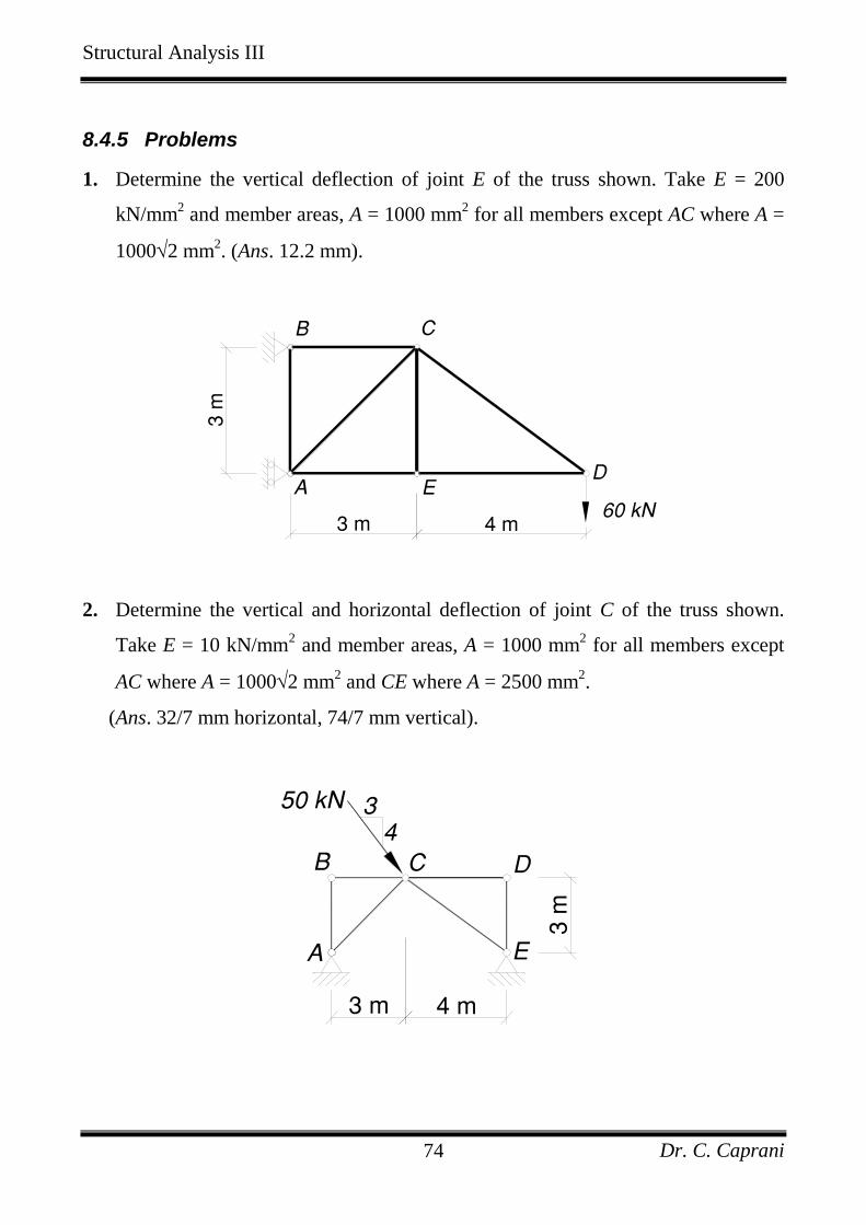
8.4.5 Problems
1. Determine the vertical deflection of joint E of the truss shown. Take E = 200
kN/mm2 and member areas, A = 1000 mm
2 for all members except AC where A =
10002 mm2. (Ans. 12.2 mm).
2. Determine the vertical and horizontal deflection of joint C of the truss shown.
Take E = 10 kN/mm2 and member areas, A = 1000 mm
2 for all members except
AC where A = 10002 mm2 and CE where A = 2500 mm
2.
(Ans. 32/7 mm horizontal, 74/7 mm vertical).
FIG. Q3
FIG. Q3(a)

Structural Analysis III
Dr. C. Caprani 75
3. Determine the horizontal deflection of joint A and the vertical deflection of joint
B of the truss shown. Take E = 200 kN/mm2 and member areas, A = 1000 mm
2
for all members except BD where A = 10002 mm2 and AB where A = 2500
mm2. (Ans. 15.3 mm; 0 mm)
4. Determine the vertical and horizontal deflection of joint C of the truss shown.
Take E = 200 kN/mm2 and member areas, A = 150 mm
2 for all members except
AC where A = 1502 mm2 and CD where A = 250 mm2. (Ans. 8.78 mm; 0.2 mm)
FIG. Q2(a)
FIG. Q3
Structural Analysis III
Dr. C. Caprani 76
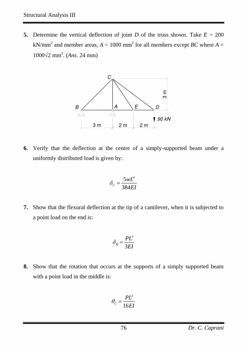
5. Determine the vertical deflection of joint D of the truss shown. Take E = 200
kN/mm2 and member areas, A = 1000 mm
2 for all members except BC where A =
10002 mm2. (Ans. 24 mm)
6. Verify that the deflection at the centre of a simply-supported beam under a
uniformly distributed load is given by:
45
384C
wL
EI
7. Show that the flexural deflection at the tip of a cantilever, when it is subjected to
a point load on the end is:
3
3B
PL
EI
8. Show that the rotation that occurs at the supports of a simply supported beam
with a point load in the middle is:
2
16C
PL
EI
FIG. Q3
Structural Analysis III
Dr. C. Caprani 77
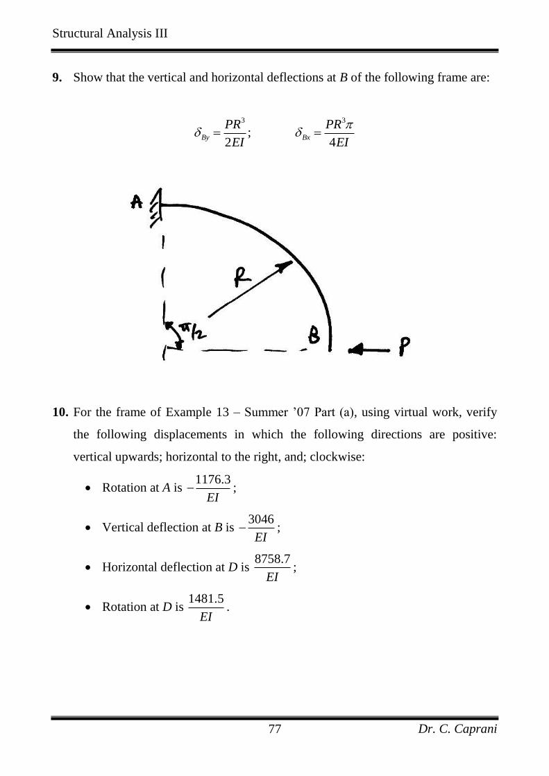
9. Show that the vertical and horizontal deflections at B of the following frame are:
3 3
;2 4
By Bx
PR PR
EI EI
10. For the frame of Example 13 – Summer ’07 Part (a), using virtual work, verify
the following displacements in which the following directions are positive:
vertical upwards; horizontal to the right, and; clockwise:
Rotation at A is 1176.3
EI ;
Vertical deflection at B is 3046
EI ;
Horizontal deflection at D is 8758.7
EI;
Rotation at D is 1481.5
EI.
Structural Analysis III
Dr. C. Caprani 78
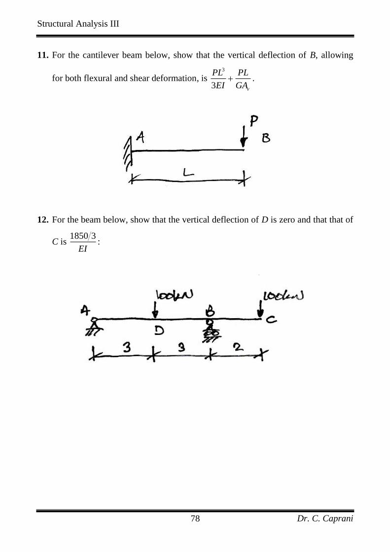
11. For the cantilever beam below, show that the vertical deflection of B, allowing
for both flexural and shear deformation, is 3
3 v
PL PL
EI GA .
12. For the beam below, show that the vertical deflection of D is zero and that that of
C is 1850 3
EI:
Structural Analysis III
Dr. C. Caprani 79
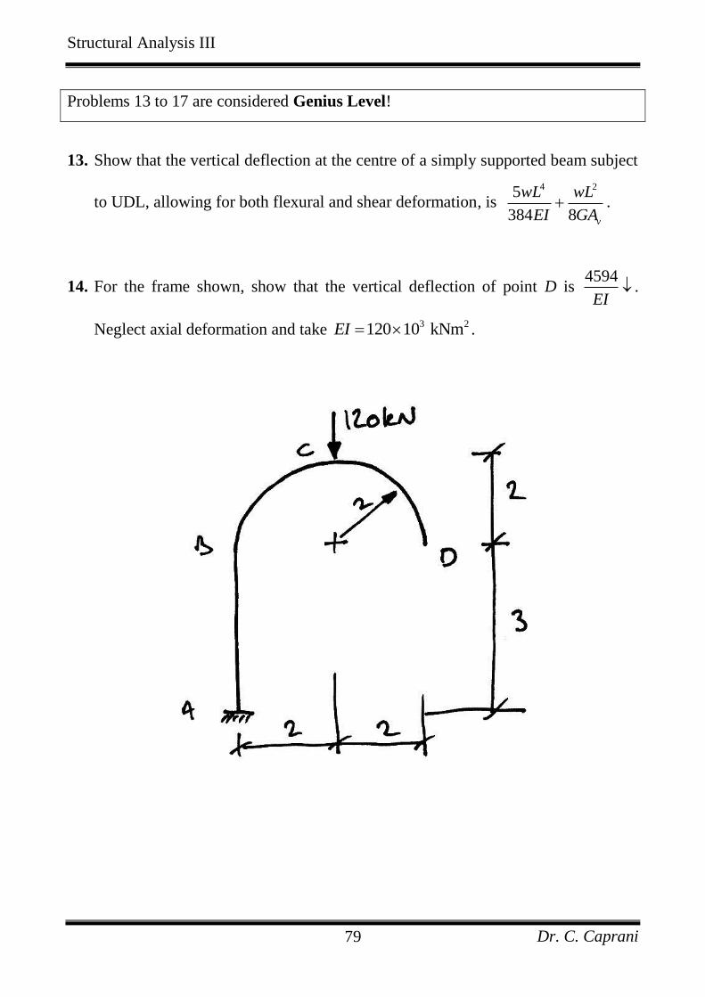
Problems 13 to 17 are considered Genius Level!
13. Show that the vertical deflection at the centre of a simply supported beam subject
to UDL, allowing for both flexural and shear deformation, is 4 25
384 8 v
wL wL
EI GA .
14. For the frame shown, show that the vertical deflection of point D is 4594
EI .
Neglect axial deformation and take 3 2120 10 kNmEI .

Structural Analysis III
Dr. C. Caprani 80
15. For the frame shown, determine the vertical deflection of C and the rotation at D
about the global x axis. Take the section and material properties as follows:
2 2 2
6 4 6 4
6600 mm 205 kN/mm 100 kN/mm
36 10 mm 74 10 mm .
A E G
I J
(Ans. 12.23 mm ; 0.0176 rads ACW)
16. Determine the horizontal and vertical deflections at B in the following frame.
Neglect shear and axial effects.
(Ans. 42
Bx
wR
EI ;
43
2By
wR
EI
)

Structural Analysis III
Dr. C. Caprani 81
17. For the frame shown, neglecting shear effects, determine the vertical deflection of
points B and A.
(Ans. 3
3By
P wa b
EI
;
33 4 21
3 8 3 2Ay
P wa bPa wa wa abPa
EI GJ
)
Structural Analysis III
Dr. C. Caprani 82
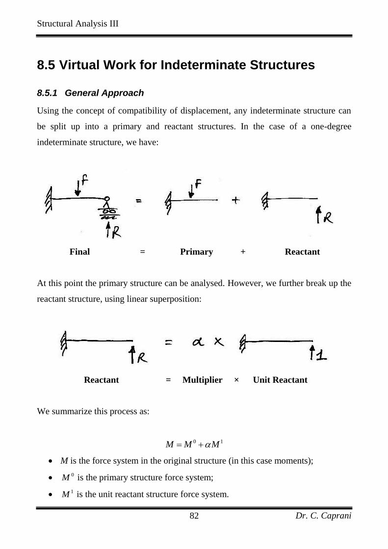
8.5 Virtual Work for Indeterminate Structures
8.5.1 General Approach
Using the concept of compatibility of displacement, any indeterminate structure can
be split up into a primary and reactant structures. In the case of a one-degree
indeterminate structure, we have:
Final = Primary + Reactant
At this point the primary structure can be analysed. However, we further break up the
reactant structure, using linear superposition:
Reactant = Multiplier × Unit Reactant
We summarize this process as:
0 1M M M
M is the force system in the original structure (in this case moments);
0M is the primary structure force system;
1M is the unit reactant structure force system.
Structural Analysis III
Dr. C. Caprani 83
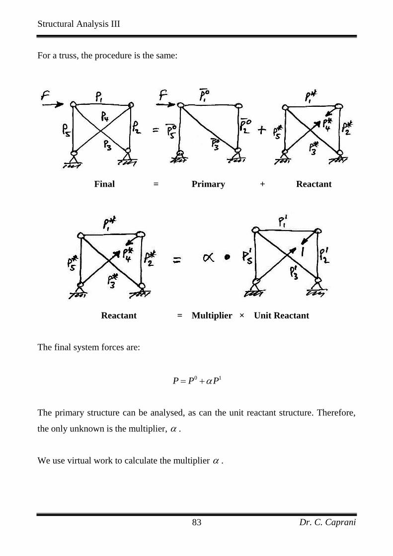
For a truss, the procedure is the same:
Final = Primary + Reactant
Reactant = Multiplier × Unit Reactant
The final system forces are:
0 1P P P
The primary structure can be analysed, as can the unit reactant structure. Therefore,
the only unknown is the multiplier, .
We use virtual work to calculate the multiplier .

Structural Analysis III
Dr. C. Caprani 84
8.5.2 Using Virtual Work to Find the Multiplier
We must identify the two sets for use:
Displacement set: We use the actual displacements that occur in the real
structure;
Equilibrium set: We use the unit reactant structure’s set of forces as the
equilibrium set. We do this, as the unit reactant is always a determinate structure
and has a configuration similar to that of the displacement set.
A typical example of these sets for an indeterminate structure is shown:
Compatibility Set Equilibrium Set
Internal and external real
displacements linked through
constitutive relations
Internal (bending moments) and external
virtual forces are linked through
equilibrium
Note that the Compatibility Set has been chosen as the real displacements of the
structure. The virtual force (equilibrium) set chosen is a statically determine sub-
structure of the original structure. This makes it easy to use statics to determine the
internal virtual ‘forces’ from the external virtual force. Lastly, note that the external
virtual force does no virtual work since the external real displacement at B is zero.
This makes the right hand side of the equation zero, allowing us to solve for the
multiplier.

Structural Analysis III
Dr. C. Caprani 85
The virtual work equation (written for trusses) gives:
1
0
0 1
E I
i i i i
i
i
W
W W
y F e P
PLP
EA
There is zero external virtual work. This is because the only virtual force applied is
internal; no external virtual force applied. Also note that the real deformations that
occur in the members are in terms of P, the unknown final forces. Hence, substituting
0 1P P P (where is now used to indicate virtual nature):
0 1
1
0 11 1
210 1
0
0
i
i
i i
i i
i ii i
i i
P P LP
EA
P L P LP P
EA EA
P LP P L
EA EA
For beams and frames, the same development is:
0
0 1
E I
i i i i
ii
W
W W
y F M
MM
EI
Where again there is no external displacement of the virtual force.
Structural Analysis III
Dr. C. Caprani 86
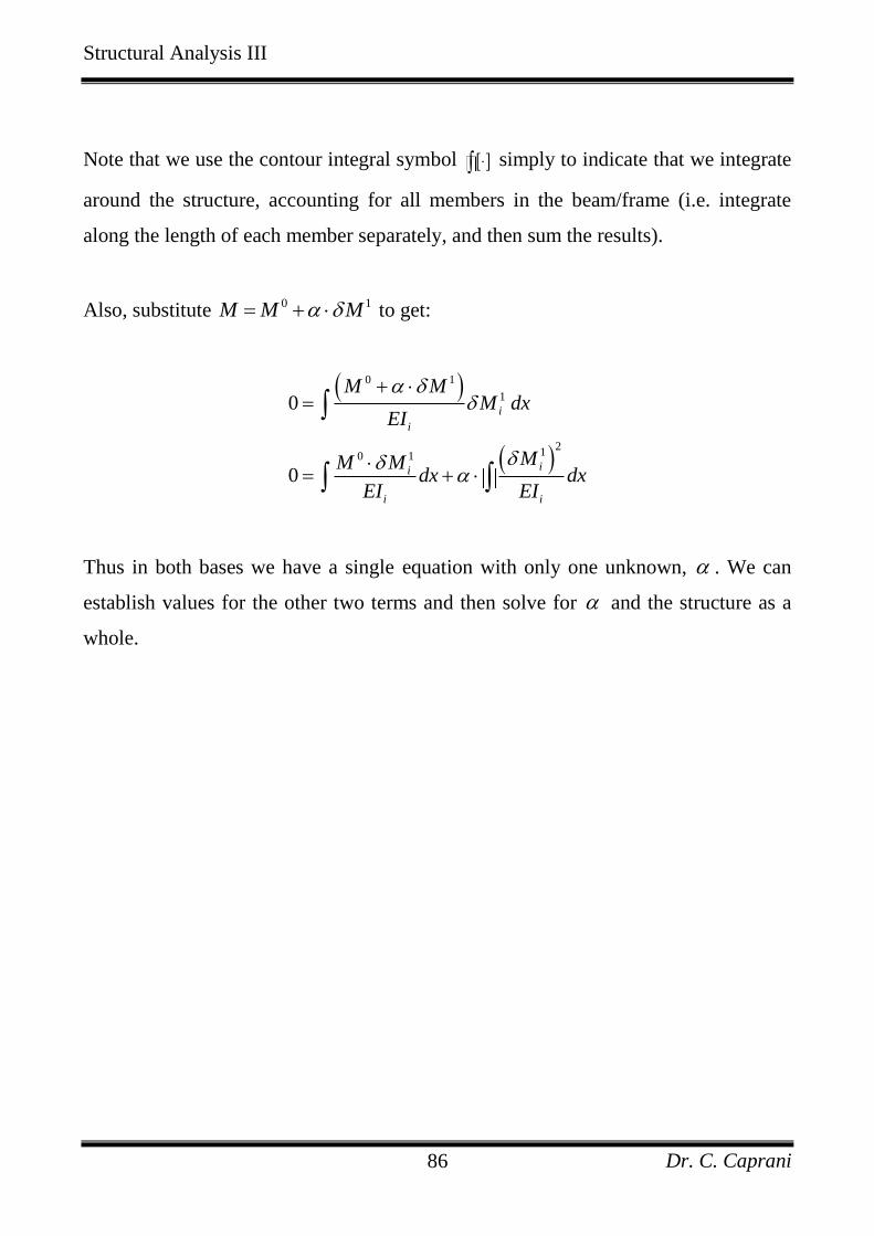
Note that we use the contour integral symbol simply to indicate that we integrate
around the structure, accounting for all members in the beam/frame (i.e. integrate
along the length of each member separately, and then sum the results).
Also, substitute 0 1M M M to get:
0 1
1
210 1
0
0
i
i
ii
i i
M MM dx
EI
MM Mdx dx
EI EI
Thus in both bases we have a single equation with only one unknown, . We can
establish values for the other two terms and then solve for and the structure as a
whole.

Structural Analysis III
Dr. C. Caprani 87
Example 14
Problem
Calculate the bending moment diagram for the following prismatic propped
cantilever. Find also the deflection under the point load.
Solution
To illustrate the methodology of selecting a redundant and analysing the remaining
determinate structure for both the applied loads ( 0M ) and the virtual unit load ( M ),
we will analyse the simple case of the propped cantilever using two different
redundants. The final solution will be the same (as it should), and this emphasis that it
does not matter which redundant is taken.
Even though the result will be the same, regardless of the redundant chosen, the
difficulty of the calculation may not be the same. As a result, a good choice of
redundant can often be made so that the ensuing calculations are made easier. A
quick qualitative assessment of the likely real and virtual bending moment diagrams
for a postulated redundant should be made, to see how the integrations will look.

Structural Analysis III
Dr. C. Caprani 88
Redundant: Vertical Reaction at B
Selecting the prop at B as the redundant gives a primary structure of a cantilever. We
determine the primary and (unit) virtual bending moment diagrams as follows:
The virtual work equation is:
2
10 1
0ii
i i
MM Mdx dx
EI EI
The terms of the virtual work equation are:
0
3
12
6 2 2 2
5
48
AC
M M PL L LEI dx L
EI
PL
2 31
3 3
M LEI dx L L L
EI
Giving:

Structural Analysis III
Dr. C. Caprani 89
3 31 5 1
048 3
PL L
EI EI
And so:
3
3
3 5 5
48 16
PL P
L
And this is the value of the reaction at B.
Redundant: Moment Reaction at A
Choosing the moment restraint at A as the redundant gives a simply-support beam as
the primary structure. The bending moments diagrams and terms of are thus:
0
2 2
2
1 1 1 12 1
6 4 2 2 3 4 2 2
2
48 48
16
AC BC
M M PL L PL LEI dx
EI
PL PL
PL

Structural Analysis III
Dr. C. Caprani 90
2
11 1
3 3
M LEI dx L
EI
Giving:
21 1
016 3
PL L
EI EI
And so:
23 3
16 16
PL PL
L
And this is the value of the moment at A.
Overall Solution
Both cases give the following overall solution, as they should:
Structural Analysis III
Dr. C. Caprani 91
8.5.3 Indeterminate Trusses
Example 15
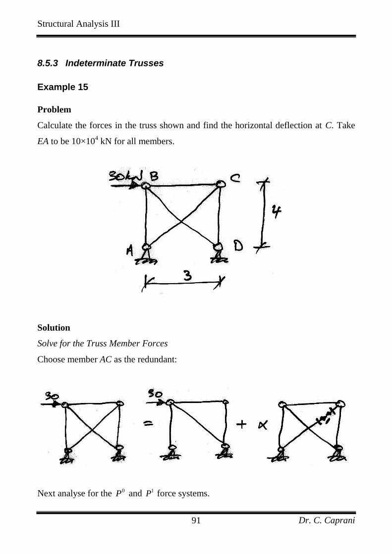
Problem
Calculate the forces in the truss shown and find the horizontal deflection at C. Take
EA to be 10×104 kN for all members.
Solution
Solve for the Truss Member Forces
Choose member AC as the redundant:
Next analyse for the 0P and 1P force systems.

Structural Analysis III
Dr. C. Caprani 92
P0 System P
1 System
Using a table:
Member L 0P
1P 0 1P P L
21P L
(mm) (kN) (kN) × 104 × 10
4
AB
BC
CD
AC
BD
4000
3000
4000
5000
5000
+40
0
0
0
-50
- 4/5
- 3/5
- 4/5
1
1
-12.8
0
0
0
-25
0.265
0.108
0.256
0.5
0.5
-37.8 1.62
Hence:
2
10 1
4 4
0
37.8 10 1.62 10
i ii i
i i
P LP P L
EA EA
EA EA

Structural Analysis III
Dr. C. Caprani 93
And so
37.823.33
1.62
The remaining forces are obtained from the compatibility equation:
Member
0P 1P
0 1P P P
(kN) (kN) (kN)
AB
BC
CD
AC
BD
+40
0
0
0
-50
- 4/5
- 3/5
- 4/5
1
1
21.36
-14
-18.67
23.33
-26.67
Note that the redundant always has a force the same as the multiplier.
Calculate the Horizontal Deflection at C
To calculate the horizontal deflection at C, using virtual work, the two relevant sets
are:
Compatibility set: the actual deflection at C and the real deformations that
occur in the actual structure;
Equilibrium set: a horizontal unit virtual force applied at C to a portion of the
actual structure, yet ensuring equilibrium.
We do not have to apply the virtual force to the full structure. Remembering that the
only requirement on the virtual force system is that it is in equilibrium; choose the
force systems as follows:

Structural Analysis III
Dr. C. Caprani 94
Thus we have:
4 4
0
1
23.33 5000 5 18.67 4000 4
10 10 3 10 10 3
2.94 mm
E I
i i i i
CH i
i
CH
W
W W
y F e P
PLy P
EA
y
Because we have chosen only two members for our virtual force system, only these
members do work and the calculation is greatly simplified.

Structural Analysis III
Dr. C. Caprani 95
8.5.4 Indeterminate Frames
Example 16
Problem
For the prismatic frame shown, calculate the reactions and draw the bending moment
diagram. Determine the vertical deflection at joint A.
Solution
Choosing the horizontal reaction at C as the redundant gives the primary structure as:

Structural Analysis III
Dr. C. Caprani 96
And the unit redundant structure as:
The terms of the virtual work equation are:
0
2
180 3 5 400
3
1 13 3 5 3 3 3 24
3 3
BC
BC BD
M MEI dx
EI
MEI dx
EI
Giving:
20
0
400 24
MM Mdx dx
EI EI
EI EI
And so the multiplier on the unit redundant is:
40016.7
24

Structural Analysis III
Dr. C. Caprani 97
As a result, using superposition of the primary and unit redundant times the multiplier
structures, we have:
To determine the deflection at A, we must apply a unit vertical virtual force at A to
obtain the second virtual force system, 2M . However, to ease the computation, and
since we only require an equilibrium system, we apply the unit vertical force to the
primary structure subset of the overall structure as follows:
The deflection is then got from the virtual work equation as follows:
2
1M M
EI

Structural Analysis III
Dr. C. Caprani 98
1 1 1
80 2 2 30 2 53 3
620 3
AB BCEI
EI
Structural Analysis III
Dr. C. Caprani 99
Example 17
Problem
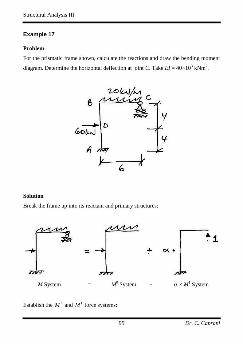
For the prismatic frame shown, calculate the reactions and draw the bending moment
diagram. Determine the horizontal deflection at joint C. Take EI = 40×103 kNm
2.
Solution
Break the frame up into its reactant and primary structures:
M System = M0 System + × M
1 System
Establish the 0M and 1M force systems:

Structural Analysis III
Dr. C. Caprani 100
M0 System M
1 System
Apply the virtual work equation:
2
10 1
0ii
i i
MM Mdx dx
EI EI
We will be using the table of volume integrals to quicken calculations. Therefore we
can only consider lengths of members for which the correct shape of bending moment
diagram is available. Also, we must choose sign convention: we consider tension on
the outside of the frame to be positive.
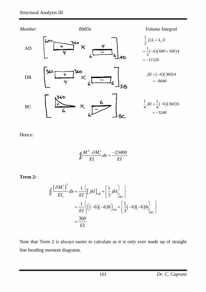
As each term has several components we consider them separately:
Term 1 - 0 1
i
i
M Mdx
EI
:
We show the volume integrals beside the real and virtual bending moment diagrams
for each member of the frame:
Structural Analysis III
Dr. C. Caprani 101
Member BMDs Volume Integral
AD
1 2
1
2
16 600 360 4
2
11520
j k k l
DB
6 360 4
8640
jkl
BC
1 1
6 360 64 4
3240
jkl
Hence:
0 1 23400i
i
M Mdx
EI EI
Term 2:
21
1 1
3
1 16 6 8 6 6 6
3
360
i
ABBCi
ABBC
Mdx jkl jkl
EI EI
EI
EI
Note that Term 2 is always easier to calculate as it is only ever made up of straight
line bending moment diagrams.
Structural Analysis III
Dr. C. Caprani 102
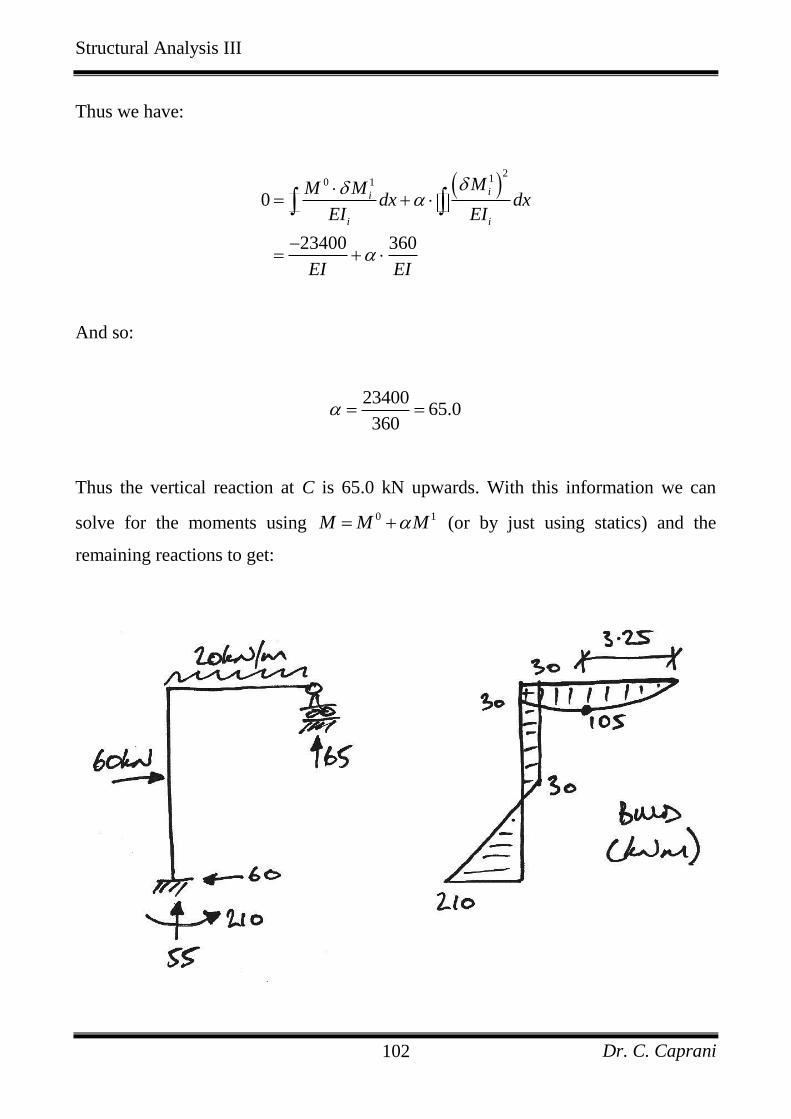
Thus we have:
2
10 1
0
23400 360
ii
i i
MM Mdx dx
EI EI
EI EI
And so:
23400
65.0360
Thus the vertical reaction at C is 65.0 kN upwards. With this information we can
solve for the moments using 0 1M M M (or by just using statics) and the
remaining reactions to get:

Structural Analysis III
Dr. C. Caprani 103
To calculate the horizontal deflection at C using virtual work, the two relevant sets
are:
Compatibility set: the actual deflection at C and the real deformations
(rotations) that occur in the actual structure;
Equilibrium set: a horizontal unit virtual force applied at C to a determinate
portion of the actual structure.
Choose the following force system as it is easily solved:
Thus we have:
0
1
E I
i i i i
xCH x
W
W W
y F M
My M dx
EI

Structural Analysis III
Dr. C. Caprani 104
The real bending moment diagram, M, is awkward to use with the integral table.
Remembering that 0 1M M M simplifies the calculation by using:
To give:
And so using the table formulae, we have:
Structural Analysis III
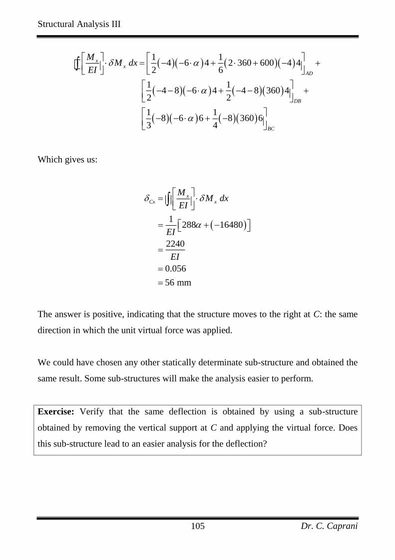
Dr. C. Caprani 105
1 14 6 4 2 360 600 4 4
2 6
1 14 8 6 4 4 8 360 4
2 2
1 18 6 6 8 360 6
3 4
xx
AD
DB
BC
MM dx
EI
Which gives us:
1
288 16480
2240
0.056
56 mm
xCx x
MM dx
EI
EI
EI
The answer is positive, indicating that the structure moves to the right at C: the same
direction in which the unit virtual force was applied.
We could have chosen any other statically determinate sub-structure and obtained the
same result. Some sub-structures will make the analysis easier to perform.
Exercise: Verify that the same deflection is obtained by using a sub-structure
obtained by removing the vertical support at C and applying the virtual force. Does
this sub-structure lead to an easier analysis for the deflection?

Structural Analysis III
Dr. C. Caprani 106
8.5.5 Multiply-Indeterminate Structures
Basis
In this section we will introduce structures that are more than 1 degree statically
indeterminate. We do so to show that virtual work is easily extensible to multiply-
indeterminate structures, and also to give a method for such beams that is easily
worked out, and put into a spreadsheet.
Consider the example 3-span beam. It is 2 degrees indeterminate, and so we introduce
2 hinges (i.e. moment releases) at the support locations and unit reactant moments in
their place, as shown:
Structural Analysis III
Dr. C. Caprani 107
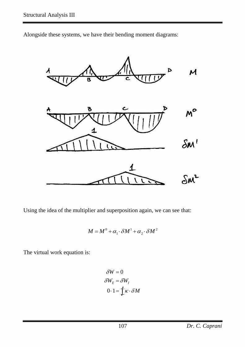
Alongside these systems, we have their bending moment diagrams:
Using the idea of the multiplier and superposition again, we can see that:
0 1 2
1 2M M M M
The virtual work equation is:
0
0 1
E I
W
W W
M

Structural Analysis III
Dr. C. Caprani 108
There is no external virtual work done since the unit moments are applied internally.
Since we have two virtual force systems in equilibrium and one real compatible
system, we have two equations:
10M
MEI
and 20M
MEI
For the first equation, expanding the expression for the real moment system, M:
0 1 2
1 2 1
0 1 1 1 2 1
1 2
0
0
M M MM
EI
M M M M M M
EI EI EI
In which we’ve dropped the contour integral – it being understood that we sum for all
members. Similarly for the second virtual moments, we have:
0 2 1 2 2 2
1 2 0M M M M M M
EI EI EI
Thus we have two equations and so we can solve for 1 and 2 . Usually we write
this as a matrix equation:
0 1 1 1 2 1
1
0 2 1 2 2 22
0
0
M M M M M M
EI EI EI
M M M M M M
EI EI EI
Each of the integral terms is easily found using the integral tables, and the equation
solved.

Structural Analysis III
Dr. C. Caprani 109
Similarly the (simpler) equation for a 2-span beam is:
0 1 1 1
1 0M M M M
EI EI
And the equation for a 4-span beam is:
0 1 1 1 2 1
10 2 1 2 2 2 3 2
2
0 3 2 3 3 3 3
0
0
0
0
0
M M M M M M
EI EI EI
M M M M M M M M
EI EI EI EI
M M M M M M
EI EI EI
The diagram shows why there are no terms involving 3 1M M , and why it is only
adjacent spans that have non-zero integrals:
Structural Analysis III
Dr. C. Caprani 110
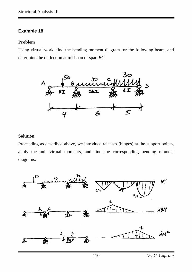
Example 18
Problem
Using virtual work, find the bending moment diagram for the following beam, and
determine the deflection at midspan of span BC.
Solution
Proceeding as described above, we introduce releases (hinges) at the support points,
apply the unit virtual moments, and find the corresponding bending moment
diagrams:

Structural Analysis III
Dr. C. Caprani 111
Next we need to evaluate each term in the matrix virtual work equation. We’ll take
the two ‘hard’ ones first:
0 1 1 1 1 150 1 4 2 45 1 6
6 2 3
1 9550 45
AB BC
M M
EI EI EI
EI EI
Note that since 1 0M for span CD, there is no term for it above. Similarly, for the
following evaluation, there will be no term for span AB. Note also the 2EI term for
member BC – this could be easily overlooked.
0 2 1 1 1 145 1 6 93.75 1 5
2 3 3
1 201.2545 156.25
BC CD
M M
EI EI EI
EI EI
The following integrals are more straightforward since they are all triangles:
1 1 1 1 1 1 2.333
1 1 4 1 1 63 2 3AB BC
M M
EI EI EI EI
2 1 1 1 0.5
1 1 62 6 BC
M M
EI EI EI
1 2 0.5M M
EI EI
, since it is equal to
2 1M M
EI
by the commutative
property of multiplication.
Structural Analysis III
Dr. C. Caprani 112
2 2 1 1 1 1 2.667
1 1 6 1 1 52 3 3BC CD
M M
EI EI EI EI
With all the terms evaluated, enter them into the matrix equation:
0 1 1 1 2 1
1
0 2 1 2 2 22
0
0
M M M M M M
EI EI EI
M M M M M M
EI EI EI
To give:
1
2
95 2.333 0.5 01 1
201.25 0.5 2.667 0EI EI
And solve, as follows:
1
2
1
2
2.333 0.5 95
0.5 2.667 201.25
2.667 0.5 951
0.5 2.333 201.252.333 2.667 0.5 0.5
25.57
70.67
Now using our superposition equation for moments, 0 1 2
1 2M M M M ,
we can show that the multipliers are just the hogging support moments:
Structural Analysis III
Dr. C. Caprani 113
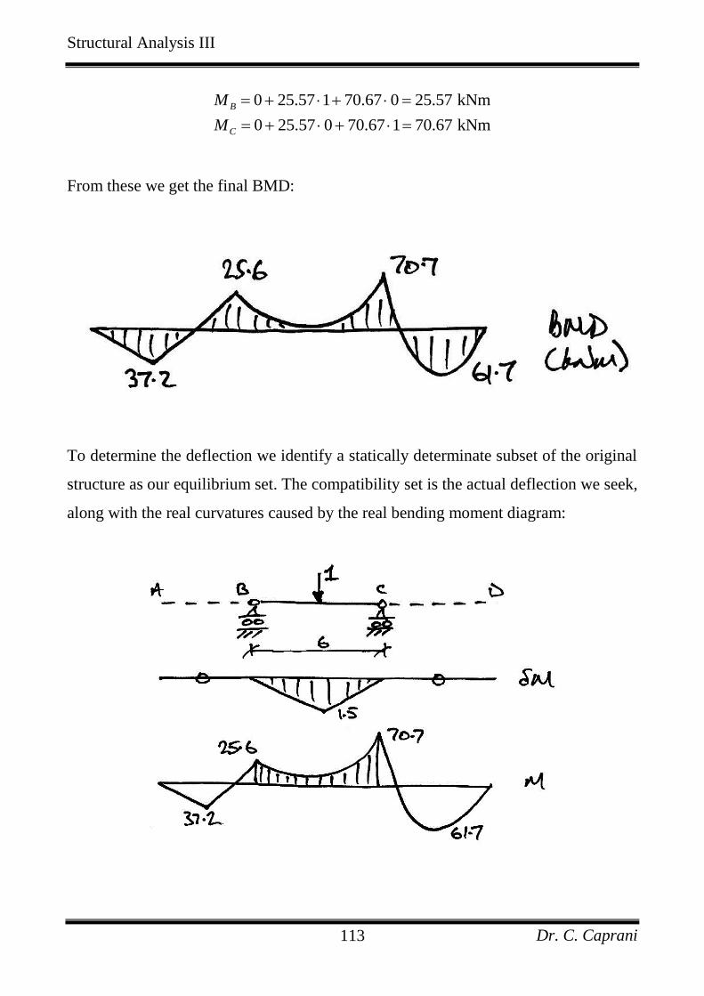
0 25.57 1 70.67 0 25.57 kNm
0 25.57 0 70.67 1 70.67 kNm
B
C
M
M
From these we get the final BMD:
To determine the deflection we identify a statically determinate subset of the original
structure as our equilibrium set. The compatibility set is the actual deflection we seek,
along with the real curvatures caused by the real bending moment diagram:

Structural Analysis III
Dr. C. Caprani 114
Notice that only the bending moment diagrams for the span being examined are
needed for the calculation. Next, we express the real bending moment diagram in
terms of its constituent parts the primary and two reactant diagrams:
And so the volume integrals are determined by multiplying the following diagrams:
Thus we have:
1 2
1 2
1 5 1 12 1.5 45 3 1.5 1 6 3 1.5 1 6 3
2 12 6 6
84.4 1.125 1.125 23.9
xx
MM dx
EI
EI
EI EI
The negative sign indicates movement opposite to the direction of the virtual unit
load and so the deflection is upwards.

Structural Analysis III
Dr. C. Caprani 115
Spreadsheet Solution
A simple spreadsheet for a 3-span beam with centre-span point load and UDL capabilities, showing Example 18, is:
Span 1 Span 2 Span 3 VW Equations
Length m 4 6 5
EI x 1 2 1 -95.000 + 2.333 0.500 * alpha1 = 0
PL kN 50 0 0 -201.250 0.500 2.667 alpha2 0
UDL kN/m 0 10 30
BMDs PL 50 0 0 2.333 0.500 * alpha1 = 95.000
UDL 0 45 93.75 0.500 2.667 alpha2 201.250
alpha1 = 0.446512 -0.083721 * 95.000
M0 x M1 Span 1 Span 2 Span 3 Totals alpha2 -0.083721 0.390698 201.250
PL -50.000 0.000 0.000
UDL 0.000 -90.000 0.000 alpha1 = 25.57
Total -50.000 -45.000 0.000 -95.000 alpha2 70.67
M1 x M1 Span 1 Span 2 Span 3
Total 1.333 1.000 0.000 2.333
Mid-Span and Support Moments
M2 x M1 Span 1 Span 2 Span 3 Mab 37.2 kNm
Total 0.000 0.500 0.000 0.500 Mb -25.6 kNm
Mbc -3.1 kNm
M0 x M2 Span 1 Span 2 Span 3 Mc -70.7 kNm
PL 0.000 0.000 0.000 Mcd 58.4 kNm
UDL 0.000 -90.000 -156.250
Total 0.000 -45.000 -156.250 -201.250
M1 x M2 Span 1 Span 2 Span 3
Total 0.000 0.500 0.000 0.500
M2 x M2 Span 1 Span 2 Span 3
Total 0.000 1.000 1.667 2.667

Structural Analysis III Chapter 8 – Virtual Work
Dr. C. Caprani 116
Example 19
Problem
Analyze the following frame for the reactions and bending moment diagram. Draw
the deflected shape of the frame.
Solution
The frame is three degrees indeterminate. We must therefore choose three
redundants. We will remove the fixed support at D to obtain the primary structure and
its bending moment diagram:

Structural Analysis III Chapter 8 – Virtual Work
Dr. C. Caprani 117
Next we apply a unit virtual force in lieu of each redundant, VD, HD, and MD, and
determine the corresponding virtual bending moment diagram:
The virtual work equation is:
0
0 1
E I
W
W W
M
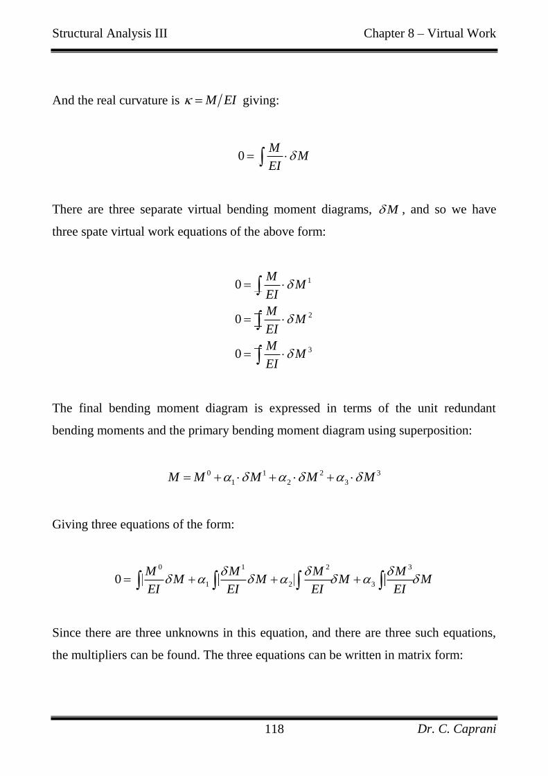
Structural Analysis III Chapter 8 – Virtual Work
Dr. C. Caprani 118
And the real curvature is M EI giving:
0M
MEI
There are three separate virtual bending moment diagrams, M , and so we have
three spate virtual work equations of the above form:
1
2
3
0
0
0
MM
EI
MM
EI
MM
EI
The final bending moment diagram is expressed in terms of the unit redundant
bending moments and the primary bending moment diagram using superposition:
0 1 2 3
1 2 3M M M M M
Giving three equations of the form:
0 1 2 3
1 2 30M M M M
M M M MEI EI EI EI
Since there are three unknowns in this equation, and there are three such equations,
the multipliers can be found. The three equations can be written in matrix form:

Structural Analysis III Chapter 8 – Virtual Work
Dr. C. Caprani 119
0 1 1 1 2 1 3 1
10 2 1 2 2 2 3 2
2
0 3 1 3 2 3 3 3 3
0
0
0
M M M M M M M M
EI EI EI EI
M M M M M M M M
EI EI EI EI
M M M M M M M M
EI EI EI EI
Virtual work problems can always be written like this. The general form of the matrix
equation is:
0
A δA α 0
where 0A is the free actions vector; δA is the virtual actions matrix; and α is
the vector of multipliers.
For this problem, we establish the terms of the free actions vector as follows:
0 1
0 2
0 3
1 18 80 6 80 6 2 2 80 2
2 3
3840 1760 3
13280 3
1 16 80 6 6 80 2
2 2
1440 480
1920
180 1 6 1 80 2
2
480 80
560
ABBC
AB BC
ABBC
M M
EI
M M
EI
M M
EI

Structural Analysis III Chapter 8 – Virtual Work
Dr. C. Caprani 120
Note that the volume integrals are commutative and so the virtual actions matrix is
symmetrical. Thus we only calculate the upper triangle terms:
1 1
2 1
3 1
2 2
1 1 18 8 6 8 8 8
3
1384 512 3
1664 3
1 1 1 16 8 6 6 8 8
2 2
1144 192
336
1 1 11 8 6 1 8 8
2
148 32
80
1
ABBC
AB BC
ABBC
M M
EI EI EI
EI
EI
M M
EI EI EI
EI
EI
M M
EI EI EI
EI
EI
M M
EI E
3 2
3 3
1 1 1 16 6 6 6 6 8 6 6 6
3 3
172 288 72
432
1 1 1 1 11 6 6 1 6 8 1 6 6
2 2
118 48 18
84
1 1 11 1 6 1 1 8 1 1 6
1
BCAB CD
BCAB CD
AB BC CD
I EI EI
EI
EI
M M
EI EI EI EI
EI
EI
M M
EI EI EI EI
E
6 8 6
20
I
EI

Structural Analysis III Chapter 8 – Virtual Work
Dr. C. Caprani 121
Substituting the values in, we obtain:
1
2
3
13280 3 1664 3 336 80 01 1
1920 336 432 84 0
560 80 84 20 0EI EI
Giving:
1
1
2
3
1664 3 336 80 13280 3 9.32 kN
336 432 84 1920 5.45 kN
80 84 20 560 13.6 kNm
This solution is easily found using software tools. For example MINVERSE and
MMULT in MS Excel, or using the following script in MATLAB, writing A0 for
0A and dA for δA :
A0 = [-13280/3; 1920; -560];
dA = [1664/3 -336 80; -336 432 -84; 80 -84 20];
a = -inv(dA)*A0;
Thus the complete solution for this problem is:
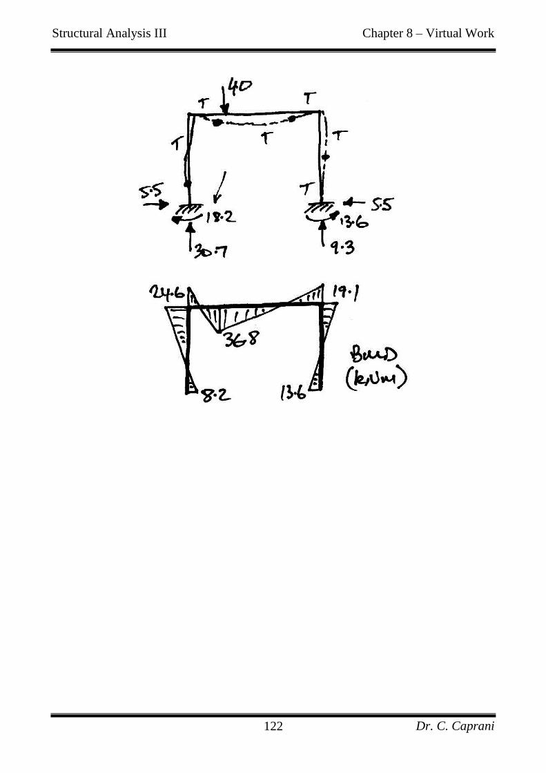
Structural Analysis III Chapter 8 – Virtual Work
Dr. C. Caprani 122

Structural Analysis III Chapter 8 – Virtual Work
Dr. C. Caprani 123
8.5.6 Problems
1. For the truss shown, calculate the vertical deflection at C when member EB is not
present and when it is present. Members AB, DC and DE have EA = 60 × 103 kN;
members EB, BC and AD have EA = 100 × 103 kN, and; member BD has EA = 80
× 103 kN. (Ans. 15 mm and 11.28 mm)
2. Calculate the vertical deflection at C when member EB is not present and when it
is present. Members AB, DC and DE have EA = 60 × 103 kN; members EB, BC
and AD have EA = 100 × 103 kN, and; member BD has EA = 80 × 10
3 kN.
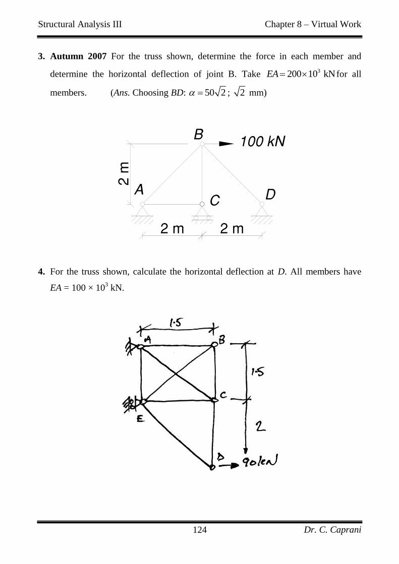
Structural Analysis III Chapter 8 – Virtual Work
Dr. C. Caprani 124
3. Autumn 2007 For the truss shown, determine the force in each member and
determine the horizontal deflection of joint B. Take 3200 10 kNEA for all
members. (Ans. Choosing BD: 50 2 ; 2 mm)
4. For the truss shown, calculate the horizontal deflection at D. All members have
EA = 100 × 103 kN.
FIG. Q3
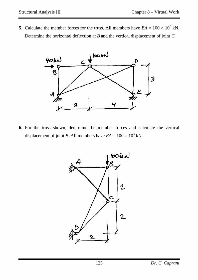
Structural Analysis III Chapter 8 – Virtual Work
Dr. C. Caprani 125
5. Calculate the member forces for the truss. All members have EA = 100 × 103 kN.
Determine the horizontal deflection at B and the vertical displacement of joint C.
6. For the truss shown, determine the member forces and calculate the vertical
displacement of joint B. All members have EA = 100 × 103 kN.

Structural Analysis III Chapter 8 – Virtual Work
Dr. C. Caprani 126
7. For the beam of Example 18, show that the deflections at the centre of the
following spans, taking downwards as positive, are:
Span AB: 41.1
EI;
Span CD: 133.72
EI.
8. For the beam shown, determine the reactions and bending moment diagram.
Determine the deflection at midspan.
9. For the beam shown, determine the reactions and bending moment diagram.
Determine the deflection at D.
10. A prestressed post-tensioned beam is shown at transfer; determine the reactions,
bending moment diagram, and deflection at midspan.

Structural Analysis III Chapter 8 – Virtual Work
Dr. C. Caprani 127
11. A prestressed post-tensioned beam is shown in service; determine the reactions,
bending moment diagram, and deflection at midspan.
12. Using virtual work, analyse the following prismatic beam to show that the support
moments are 51.3 kNmBM and 31.1 kNmCM . Draw the bending moment
diagram. Show that the deflections at middle of the spans moving left to right are
19.6/EI, 204/EI, and 71.6/EI respectively.
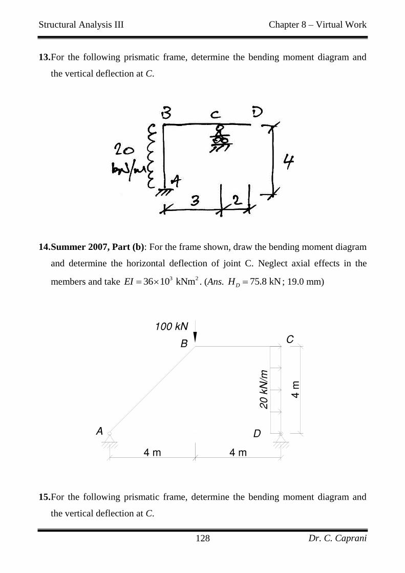
Structural Analysis III Chapter 8 – Virtual Work
Dr. C. Caprani 128
13. For the following prismatic frame, determine the bending moment diagram and
the vertical deflection at C.
14. Summer 2007, Part (b): For the frame shown, draw the bending moment diagram
and determine the horizontal deflection of joint C. Neglect axial effects in the
members and take 3 236 10 kNmEI . (Ans. 75.8 kNDH ; 19.0 mm)
15. For the following prismatic frame, determine the bending moment diagram and
the vertical deflection at C.
FIG. Q3(b)

Structural Analysis III Chapter 8 – Virtual Work
Dr. C. Caprani 129
16. For the following prismatic frame, determine the bending moment diagram and
the vertical deflection at C.
17. For the following prismatic frame, determine the bending moment diagram and
the vertical deflection at C.

Structural Analysis III Chapter 8 – Virtual Work
Dr. C. Caprani 130
18. For the following prismatic portal frame, determine the bending moment diagram
and the horizontal deflection at B and D.
19. For the frame shown, calculate the bending moment diagram, and verify the
following deflections: 856.2
BxEI
and 327.6
CyEI
. (Ans. 30.1 kNmBM )
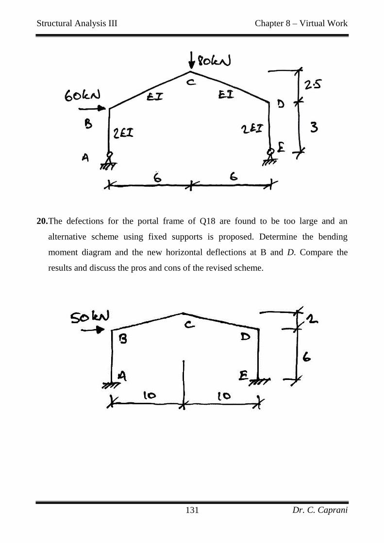
Structural Analysis III Chapter 8 – Virtual Work
Dr. C. Caprani 131
20. The defections for the portal frame of Q18 are found to be too large and an
alternative scheme using fixed supports is proposed. Determine the bending
moment diagram and the new horizontal deflections at B and D. Compare the
results and discuss the pros and cons of the revised scheme.
Structural Analysis III Chapter 8 – Virtual Work
Dr. C. Caprani 132
8.6 Virtual Work for Self-Stressed Structures
8.6.1 Background
Introduction
Self-stressed structures are structures that have stresses induced, not only by external
loading, but also by any of the following:
Temperature change of some of the members (e.g. solar gain);
Lack of fit of members from fabrication:
o Error in the length of the member;
o Ends not square and so a rotational lack of fit;
Incorrect support location from imperfect construction;
Non-rigid (i.e. spring) supports due to imperfect construction.
Since any form of fabrication or construction is never perfect, it is very important for
us to know the effect (in terms of bending moment, shear forces etc.) that such errors,
even when small, can have on the structure.
Here we introduce these sources, and examine their effect on the virtual work
equation. Note that many of these sources of error can exist concurrently. In such
cases we add together the effects from each source.

Structural Analysis III Chapter 8 – Virtual Work
Dr. C. Caprani 133
Temperature Change – Axial
The source of self-stressing in this case is that the temperature change causes a
member to elongate:
TL L T
where is the coefficient of linear thermal expansion (change in length, per unit
length, per degree Celsius), L is the original member length and T is the
temperature change.
Since temperature changes change the length of a member, the internal virtual work
is affected. Assuming a truss member is being analysed, we now have changes in
length due to force and temperature, so the total change in length of the member is:
PL
e L TEA
Hence the internal virtual work for this member is:
IW e P
PLL T P
EA

Structural Analysis III Chapter 8 – Virtual Work
Dr. C. Caprani 134
Temperature Change – Curvature
When two sides of a flexural member are exposed to different temperature changes,
both an axial elongation and curvature result. A typical example is a bridge deck: the
road surface is exposed to the sun and heats up whilst the underside (soffit) is not
exposed to directly sunlight and so heats less.
A short element of the member, dx, which has depth h, expands as shown. This
deformation can be broken up into axial ( eT ) and flexural ( T ) components:
Hence the curvature at the section is:
2
x
Tdx
h

Structural Analysis III Chapter 8 – Virtual Work
Dr. C. Caprani 135
In terms of the change in temperature at the top and bottom of the beam, we have:
2
t bT TT
And so:
t bx
T Tdx
h
Since the virtual work done by a virtual moment moving through this real curvature
at the cross section is:
IW M
These expressions are valid for a point along the beam. Hence, along the full length
of the member, the virtual work done is:
0 0
L L
I x x t b xW M dx T T M dxh
If we assume that the member is prismatic and the temperature changes are the same
long the length of the beam, we have:
0
L
I t b xW T T M dxh
Which is just t bT T h times the area under the virtual moment diagram.
Structural Analysis III Chapter 8 – Virtual Work
Dr. C. Caprani 136
Linear Lack of Fit
For a linear lack of fit, the member needs to be artificially elongated or shortened to
fit it into place, thus introducing additional stresses. This is denoted:
L
Considering a truss member subject to external loading, the total change in length
will be the deformation due to loading and the linear lack of fit:
L
PLe
EA
Hence the internal virtual work for this member is:
I
L
W e P
PLP
EA
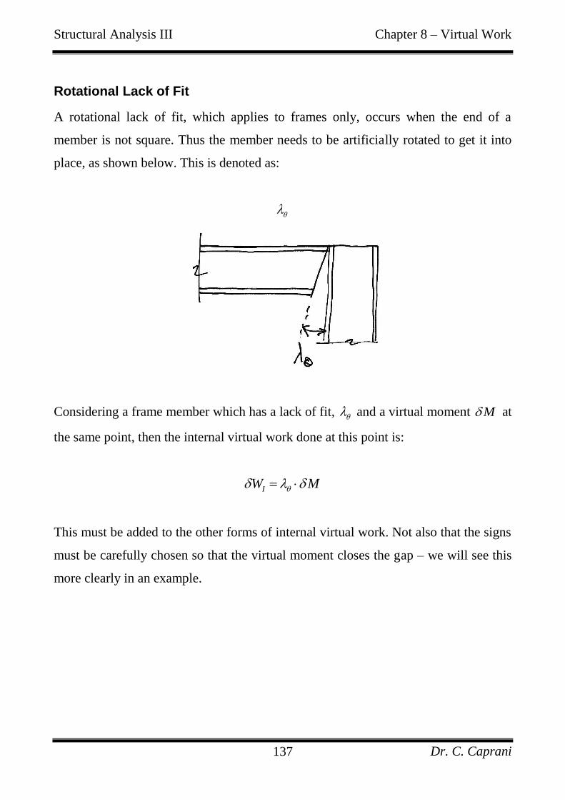
Structural Analysis III Chapter 8 – Virtual Work
Dr. C. Caprani 137
Rotational Lack of Fit
A rotational lack of fit, which applies to frames only, occurs when the end of a
member is not square. Thus the member needs to be artificially rotated to get it into
place, as shown below. This is denoted as:
Considering a frame member which has a lack of fit, and a virtual moment M at
the same point, then the internal virtual work done at this point is:
IW M
This must be added to the other forms of internal virtual work. Not also that the signs
must be carefully chosen so that the virtual moment closes the gap – we will see this
more clearly in an example.

Structural Analysis III Chapter 8 – Virtual Work
Dr. C. Caprani 138
Errors in Support Location
The support can be misplaced horizontally and/or vertically. It is denoted:
S
A misplaced support affects the external movements of a structure, and so contributes
to the external virtual work. Denoting the virtual reaction at the support, in the
direction of the misplacement as R , then we have:
e SW R

Structural Analysis III Chapter 8 – Virtual Work
Dr. C. Caprani 139
Spring Supports
For spring supports we will know the spring constant for the support, denoted:
Sk
Since movements of a support are external, spring support movements affect the
external virtual work. The real displacement S that occurs is:
S SR k
In which R is the real support reaction in the direction of the spring. Further, since R
will be known in terms of the multiplier and virtual reaction, R , we have:
0R R R
Hence:
0
S SR R k
And so the external work done is:
20
e S
S S
W R
RRR
k k
The only unknown here is which is solved for from the virtual work equation.

Structural Analysis III Chapter 8 – Virtual Work
Dr. C. Caprani 140
8.6.2 Trusses
Example 20
Problem
Here we take the truss of Example 7 and examine the effects of:
Member ED was found to be 5 mm too long upon arrival at site;
Member AB is subject to a temperature increase of +100 ˚C.
For this truss, E = 200 kN/mm2;
member areas, A = 1000 mm2 for all members except
AE and BD where A = 10002 mm2, and; coefficient of thermal expansion is
6 -110 10 C .
Solution
The change in length due to the temperature change is:
610 10 2000 100
2 mm
TL L T
Structural Analysis III Chapter 8 – Virtual Work
Dr. C. Caprani 141
Vertical Displacement of Joint D
The virtual work equation is now:
01 1 1
0
1 5 2
E I
i i i i
DV i ED AB
i
W
W W
y F e P
P Ly P P P
EA
In Example 7 we established various values in this equation:
0
1 16.5i
i
P LP
EA
1 1EDP
1 1ABP
Hence we have:
1 16.5 5 1 2 1
13.5 mm
DV
DV
y
y
Horizontal Displacement of Joint D:
Similarly, taking the values obtained in Example 7, we have:
02 2 21 5 2
4.5 5 1 2 0
0.5 mm to the right
DH i ED AB
i
DH
P Ly P P P
EA
y

Structural Analysis III Chapter 8 – Virtual Work
Dr. C. Caprani 142
Example 21
Problem
Here we use the truss of Example 15 and examine, separately, the effects of:
Member AC was found to be 3.6 mm too long upon arrival on site;
Member BC is subject to a temperature reduction of -50 ˚C;
Support D is surveyed and found to sit 5 mm too far to the right.
Take EA to be 10×104 kN for all members and the coefficient of expansion to be
6 -110 10 C .
Solution
Error in Length:
To find the new multiplier, we include this effect in the virtual work equation:
1 1
0
0
E I
i i i i
i L AC
i
W
W W
y F e P
PLP P
EA
Structural Analysis III Chapter 8 – Virtual Work
Dr. C. Caprani 143
But 0 1P P P , hence:
0 1
1 1
0 11 1 1
210 1
1
0
0
i L AC
i
i i L AC
i i
i ii iL AC
i i
P P LP P
EA
P L P LP P P
EA EA
P LP P LP
EA EA
As can be seen, the 1
L ACP term is simply added to the usual VW equation. From
before, we have the various values of the summations, and so have:
4 437.8 10 1.62 10
0 3.6 1EA EA
4
4
37.8 10 3.61.11
1.62 10
EA
Thus member AC is 1.1 kN in tension. Note the change: without the error in fit it was
23.3 kN in tension and so the error in length has reduced the tension by 22.2 kN.
Temperature Change:
The same derivation from the VW equation gives us:
2
10 110
i ii iT BC
i i
P LP P LL P
EA EA
The change in length due to the temperature change is:
Structural Analysis III Chapter 8 – Virtual Work
Dr. C. Caprani 144
610 10 3000 50 1.5 mm
TL L T
Noting that the virtual force in member BC is 1 0.6BCP , we have:
4 437.8 10 1.62 10
0 1.5 0.6EA EA
Giving:
4
4
37.8 10 0.917.7
1.62 10
EA
Thus member AC is 17.7 kN in tension, a decrease of 5.6 kN from 23.3 kN.
Error in Support Location:
Modifying the VW equation gives:
2
10 1i ii i
S D
i i
P LP P LH
EA EA
The value of the virtual horizontal reaction is found from the virtual force system to
be 0.6 kN to the right. Hence:
4 437.8 10 1.62 10
5 0.6EA EA
Structural Analysis III Chapter 8 – Virtual Work
Dr. C. Caprani 145
Note the sign on the support displacement: since the real movement is along the same
direction as the virtual force, it does positive virtual work. Solving:
4
4
3 37.8 104.8
1.62 10
EA
Thus member AC is 4.8 kN in tension; a reduction of 18.5 kN.
All Effects Together:
In this case, the virtual work equation is:
2
10 11 1i ii i
S D L AC T BC
i i
P LP P LH P L P
EA EA
Substituting the various values in gives:
4 437.8 10 1.62 10
5 0.6 3.6 1 1.5 0.6EA EA
And solving:
4
4
3.6 0.9 3 37.8 1022.9
1.62 10
EA
And so member AC is 22.9 kN in compression. Thus should be the same as the
original force of 23.3 kN plus all the changes induced by the errors:
23.3 22.2 5.6 18.5 23.0 kN
Structural Analysis III Chapter 8 – Virtual Work
Dr. C. Caprani 146
Exercise: Find the remaining forces in the truss and compare to the forces without
the presence of self-stresses and calculate the horizontal deflection at C without self-
stresses.

Structural Analysis III Chapter 8 – Virtual Work
Dr. C. Caprani 147
8.6.3 Beams
Example 22
Problem
Determine the deflection at the centre of a simply-supported beam subject to a linear
temperature increase over the section depth:
Solution
We will assume that 2 1T T for developing the solution, and consider positive
displacements to be upwards consequently. We identify the compatibility set as the
real internal and external displacements:
Next, we identify the equilibrium set, which is the external virtual force and internal
virtual bending moments:

Structural Analysis III Chapter 8 – Virtual Work
Dr. C. Caprani 148
The curvature is constant, since the temperature changes are constant along the length
of the beam. Thus the virtual work equation is:
2 1
0
1 x
L
x
M dx
T T M dxh
The area under the virtual moment diagram is 20.5 4 8L L L . Hence we have
the solution as:
2
2 18
LT T
h
Numerical Example
If we take the following values:
2 50 CT ;
1 20 CT ;
L = 10 m;
6 -110 10 C ;
h = 500 mm

Structural Analysis III Chapter 8 – Virtual Work
Dr. C. Caprani 149
Then we have:
26 310 10 10 10
50 20 7.5 mm8 500
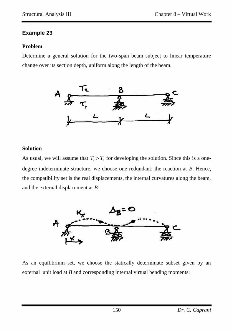
Structural Analysis III Chapter 8 – Virtual Work
Dr. C. Caprani 150
Example 23
Problem
Determine a general solution for the two-span beam subject to linear temperature
change over its section depth, uniform along the length of the beam.
Solution
As usual, we will assume that 2 1T T for developing the solution. Since this is a one-
degree indeterminate structure, we choose one redundant: the reaction at B. Hence,
the compatibility set is the real displacements, the internal curvatures along the beam,
and the external displacement at B:
As an equilibrium set, we choose the statically determinate subset given by an
external unit load at B and corresponding internal virtual bending moments:

Structural Analysis III Chapter 8 – Virtual Work
Dr. C. Caprani 151
Next we write the general virtual work equation, noting the external unit load moves
through no virtual displacement:
1 0 x M dx
And establish that the real curvatures are made up of both temperature-induced
curvatures and load (or bending moment)-induced curvatures:
x T M
But we know the temperature curvature to be constant, and causes tension on top so
we have:
2 1T T Th
And the moment (or load)-induced curvature is found as usual:
0M
M M R M
EI EI
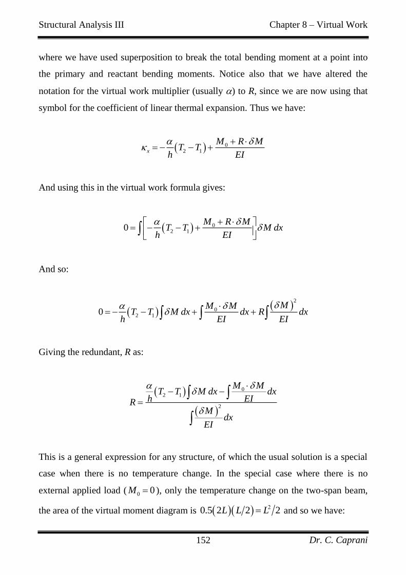
Structural Analysis III Chapter 8 – Virtual Work
Dr. C. Caprani 152
where we have used superposition to break the total bending moment at a point into
the primary and reactant bending moments. Notice also that we have altered the
notation for the virtual work multiplier (usually ) to R, since we are now using that
symbol for the coefficient of linear thermal expansion. Thus we have:
02 1x
M R MT T
h EI
And using this in the virtual work formula gives:
02 10
M R MT T M dx
h EI
And so:
2
02 10
MM MT T M dx dx R dx
h EI EI
Giving the redundant, R as:
02 1
2
M MT T M dx dx
h EIRM
dxEI
This is a general expression for any structure, of which the usual solution is a special
case when there is no temperature change. In the special case where there is no
external applied load ( 0 0M ), only the temperature change on the two-span beam,
the area of the virtual moment diagram is 0.5 2 2 2L L L and so we have:

Structural Analysis III Chapter 8 – Virtual Work
Dr. C. Caprani 153
2
2 1
2 1
321 1
23 2 2
LT T
EIhR T TL L L h
LEI
In which we have used the volume integral for the triangular virtual bending moment
diagram.
Numerical Example
If we take the following values:
2 50 CT ;
1 20 CT ;
L = 10 m;
6 -110 10 C ;
h = 500 mm;
3 240 10 kNmEI
Then we have:
3 63 40 10 10 10
50 20 7.2kN10 0.5
R
And there is a bending moment across the beam as follows:
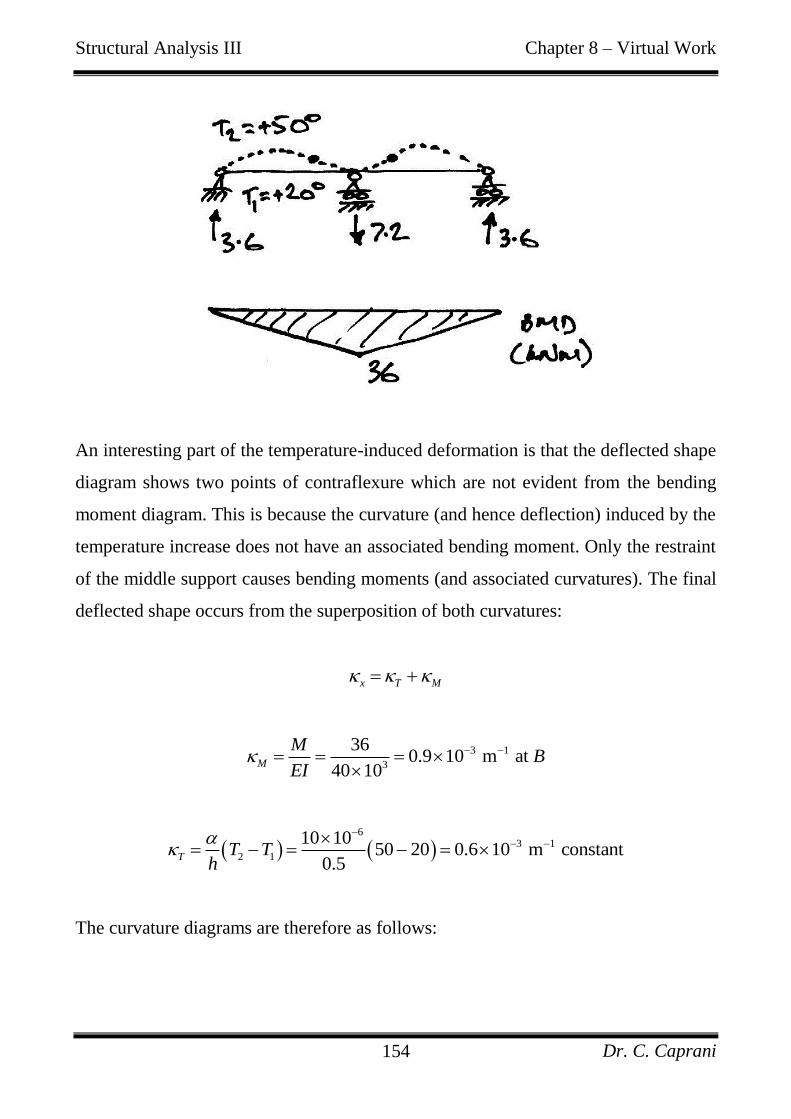
Structural Analysis III Chapter 8 – Virtual Work
Dr. C. Caprani 154
An interesting part of the temperature-induced deformation is that the deflected shape
diagram shows two points of contraflexure which are not evident from the bending
moment diagram. This is because the curvature (and hence deflection) induced by the
temperature increase does not have an associated bending moment. Only the restraint
of the middle support causes bending moments (and associated curvatures). The final
deflected shape occurs from the superposition of both curvatures:
x T M
3 1
3
360.9 10 m at
40 10M
MB
EI
6
3 1
2 1
10 1050 20 0.6 10 m constant
0.5T T T
h
The curvature diagrams are therefore as follows:

Structural Analysis III Chapter 8 – Virtual Work
Dr. C. Caprani 155

Structural Analysis III Chapter 8 – Virtual Work
Dr. C. Caprani 156
Example 24
Problem
Consider the following 2-span beam with central spring support. Determine an
expression for the central support reaction in terms of its spring stiffness.
Solution
To do this, we will consider the central support as the redundant:
The virtual work equation, accounting for the spring, is:
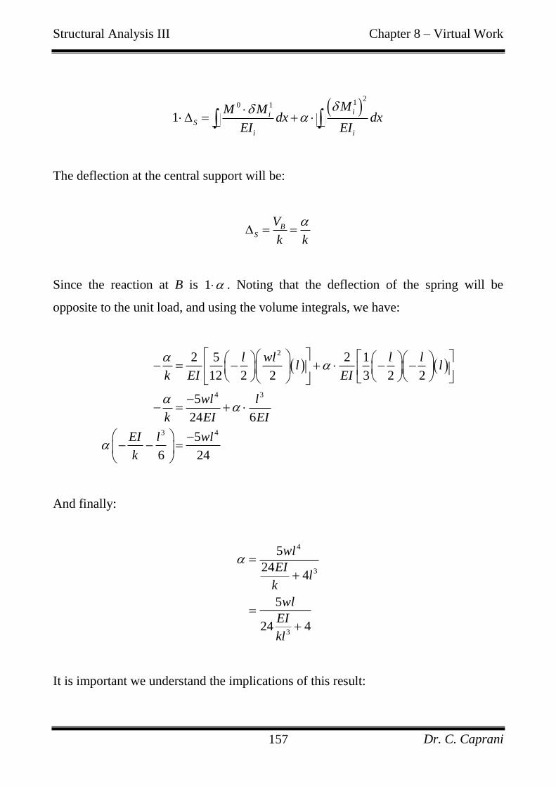
Structural Analysis III Chapter 8 – Virtual Work
Dr. C. Caprani 157
2
10 1
1ii
S
i i
MM Mdx dx
EI EI
The deflection at the central support will be:
BS
V
k k
Since the reaction at B is 1 . Noting that the deflection of the spring will be
opposite to the unit load, and using the volume integrals, we have:
2
4 3
3 4
2 5 2 1
12 2 2 3 2 2
5
24 6
5
6 24
l wl l ll l
k EI EI
wl l
k EI EI
EI l wl
k
And finally:
4
3
3
5
244
5
24 4
wl
EIl
k
wl
EI
kl
It is important we understand the implications of this result:
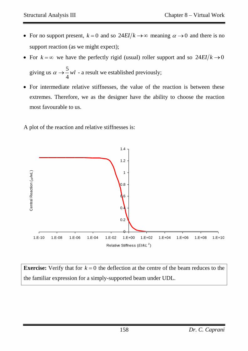
Structural Analysis III Chapter 8 – Virtual Work
Dr. C. Caprani 158
For no support present, 0k and so 24EI k meaning 0 and there is no
support reaction (as we might expect);
For k we have the perfectly rigid (usual) roller support and so 24 0EI k
giving us 5
4wl - a result we established previously;
For intermediate relative stiffnesses, the value of the reaction is between these
extremes. Therefore, we as the designer have the ability to choose the reaction
most favourable to us.
A plot of the reaction and relative stiffnesses is:
Exercise: Verify that for 0k the deflection at the centre of the beam reduces to the
the familiar expression for a simply-supported beam under UDL.
0
0.2
0.4
0.6
0.8
1
1.2
1.4
1.E-10 1.E-08 1.E-06 1.E-04 1.E-02 1.E+00 1.E+02 1.E+04 1.E+06 1.E+08 1.E+10
Relative Stiffness (EI/kL3)
Ce
ntr
al R
ea
ctio
n (
/wL
)

Structural Analysis III Chapter 8 – Virtual Work
Dr. C. Caprani 159
Example 25
Problem
A simply supported beam has a rotational lack of fit at midspan as shown. Determine
the deflection at midspan.
Solution
We apply a unit virtual load at midspan. The virtual work equation is:
1 C C
M Mdx M
EI
The first term returns the deflection due to the loading alone. The second term
accounts for the lack of fit. Note that the work done is positive when closing a lack of
fit. In this case, the applied virtual moment opens the lack of fit and so this term is
negative overall. From the usual real and virtual bending moment diagrams, we have:
2
4
1 52
12 8 4 2 4
5
384 4
C
wL L L L
EI
wL L
EI
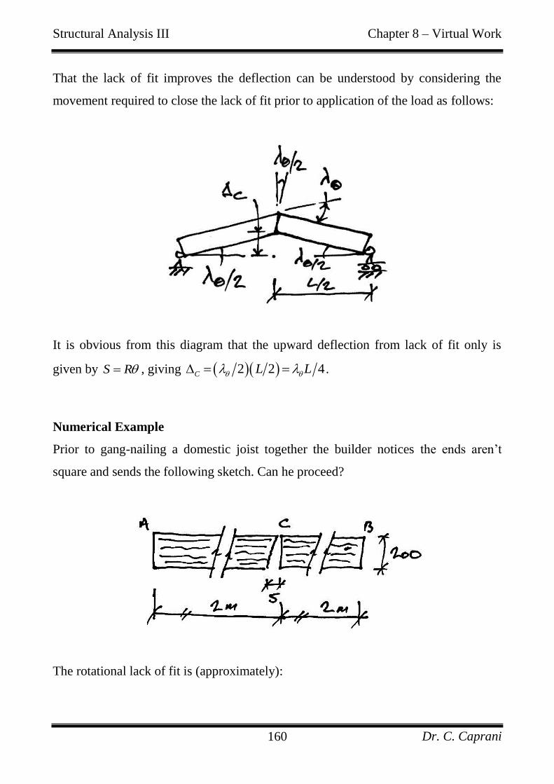
Structural Analysis III Chapter 8 – Virtual Work
Dr. C. Caprani 160
That the lack of fit improves the deflection can be understood by considering the
movement required to close the lack of fit prior to application of the load as follows:
It is obvious from this diagram that the upward deflection from lack of fit only is
given by S R , giving 2 2 4C L L .
Numerical Example
Prior to gang-nailing a domestic joist together the builder notices the ends aren’t
square and sends the following sketch. Can he proceed?
The rotational lack of fit is (approximately):

Structural Analysis III Chapter 8 – Virtual Work
Dr. C. Caprani 161
5
0.025 rads200
The upward displacement is thus:
30.025 4 10
25mm4
Taking a deflection limit of span/200 for a domestic case, the limit is:
3
allow
4 1020mm
200
On this analysis the builder should not proceed. However, the clever engineer can
make this work, allowing the builder to proceed – what can be taken into account to
allow this?

Structural Analysis III Chapter 8 – Virtual Work
Dr. C. Caprani 162
8.6.4 Frames
Example 26
Problem
The following frame, in addition to its loading, is subject to:
Support A is located 10 mm too far to the left;
End C of member BC is 31.2 10 rads out of square, as shown;
Member CD is 12 mm too short.
Determine the bending moment diagram. Take EI = 36 × 103 kNm
2 for each member.
Solution
We will choose the horizontal reaction at A as the redundant. Since we are dealing
with a linear lack of fit in member CD, we need to allow for the virtual work done by
the axial forces in this member and so we solve for the axial force diagrams also.
For the primary structure:
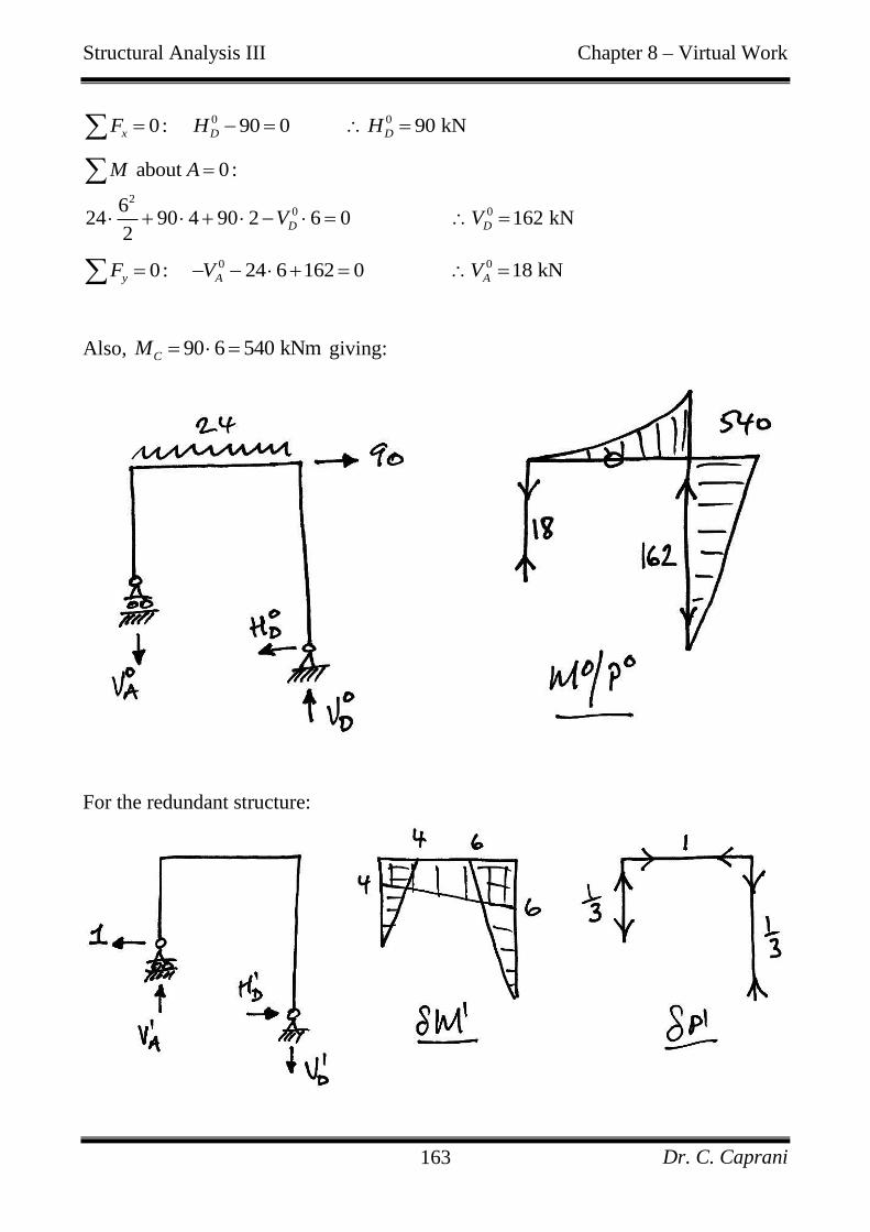
Structural Analysis III Chapter 8 – Virtual Work
Dr. C. Caprani 163
0 00: 90 0 90 kNx D DF H H
20 0
about 0 :
624 90 4 90 2 6 0 162 kN
2D D
M A
V V
0 00: 24 6 162 0 18 kNy A AF V V
Also, 90 6 540 kNmCM giving:
For the redundant structure:

Structural Analysis III Chapter 8 – Virtual Work
Dr. C. Caprani 164
1 1
1 1
1 about 0 : 1 2 6 0 kN
3
1 10 : 0 kN
3 3
D D
y A A
M A V V
F V V
The virtual work equation, accounting for the relevant effects is:
2
10 11 1 1
0
E I
iiS A C L CD
i i
W
W W
MM MH dx dx M P
EI EI
We take each term in turn:
(a) 1
S AH : The applied unit load is in the same direction as the error in the
support location, and keeping all units in metres:
1 3 310 10 1 10 10 kN mS AH
(b) 0 1
i
i
M Mdx
EI
: Using the volume integrals:
0 1 1 1 1
4 3 6 540 6 6 540 612 3
12420
i
BC CDi
M Mdx
EI EI
EI
(c)
21
i
i
Mdx
EI
: Again using the integrals table:

Structural Analysis III Chapter 8 – Virtual Work
Dr. C. Caprani 165
21
1 1 1 14 4 4 4 2 4 6 6 4 2 6 6
3 6
1 16 6 6
3
i
AB BCi
CD
Mdx
EI EI EI
EI
2
1245.33i
i
Mdx
EI EI
(d) 1
CM : The virtual bending moment at C is 6 kNm with tension on the
inside of the frame. This is in the opposite direction to that needed to close the
lack of fit and so the sign of this term is negative, as shown:
1 3 31.2 10 6 7.2 10 kN mCM
(e) 1
L CDP : Since the member is too short, the lack of fit is negative, whilst the
virtual force is in tension and so positive:
1 3 3112 10 4 10 kN m
3L CDP

Structural Analysis III Chapter 8 – Virtual Work
Dr. C. Caprani 166
Substituting these values into the equation, along with 3 236 10 kNmEI , gives:
3 3 3
3 3
12420 245.3310 10 7.2 10 4 10
36 10 36 10
And so we can solve for :
10 345 6.815 7.2 4
10 345 7.2 4
6.815
53.73
And so the horizontal reaction at A is:
0 1 0 53.73 1 53.73 kNA A AH H H
and similarly for the other reactions. Also, using the superposition equation for
moments, 0 1M M M , we have:

Structural Analysis III Chapter 8 – Virtual Work
Dr. C. Caprani 167
8.6.5 Problems
1. For the truss of Example 21, show that the force in member AC is 22.2 kN in
compression when there is no external loads present, and only the lack of fit of 3.6
mm of member AC.
2. For the truss of Example 21, determine the horizontal deflection of joint C due to
each of the errors separately, and then combined.
3. For the beam of Example 24, show that the stiffness of the spring support that
optimizes the bending moments is 389.5EI l , i.e. makes the sagging and hogging
moments equal in magnitude.
4. For the following beam, show that the vertical deflection at C can be given by:
32 1
3Cy
LP
EI k
5. For the following beam, determine the bending moment diagram. Take
6 -110 10 C , h = 500 mm, and 3 240 10 kNmEI .

Structural Analysis III Chapter 8 – Virtual Work
Dr. C. Caprani 168
6. For the following prismatic beam, determine the bending moment diagram,
reactions and midspan deflections for the lack of fit scenario shown.
7. Solve the following prismatic beam, for the bending moment diagram. Show that
the bending moment and deflection at C approaches the limiting cases for a
pinned-pinned beam and a fixed-fixed beam as k approaches 0 and infinity
respectively. You may use the symmetry of the problem in your solution.

Structural Analysis III Chapter 8 – Virtual Work
Dr. C. Caprani 169
8. For the following prismatic beam, investigate the behaviour for different ratios of
EI to the support stiffness, k. Is the reaction at C always downwards?
9. For the frame of Example 26, show that the horizontal deflection of joint C due to
the applied loads only is 77.5 mm. Find the deflection of joint C due to both the
loads and errors given.
10. For the following frame, the support at D was found to yield horizontally by 0.08
mm/kN. Also, the end of member BC is not square, as shown. Draw the bending
moment diagram and determine the horizontal deflection at D. Take EI = 100×103
kNm2. (Ans. 5.43 mm to the right)

Structural Analysis III Chapter 8 – Virtual Work
Dr. C. Caprani 170
8.7 Past Exam Questions
Summer 1997
Answers:
(a) 30.0 mmCx ;
(b) 12.9 mmCx ;
(c) 21.1 mmBD too long.

Structural Analysis III Chapter 8 – Virtual Work
Dr. C. Caprani 171
Summer 1998
Answers:
(a) 45.0 mmCx ; (b) 26.2 mmCx .
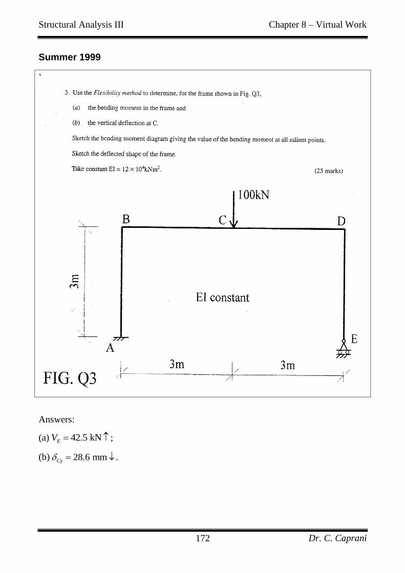
Structural Analysis III Chapter 8 – Virtual Work
Dr. C. Caprani 172
Summer 1999
‘
Answers:
(a) 42.5 kNEV ;
(b) 28.6 mmCy .
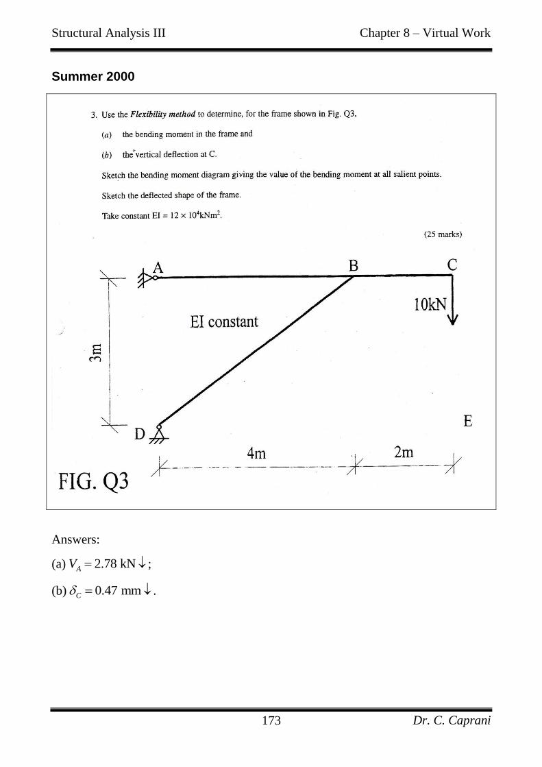
Structural Analysis III Chapter 8 – Virtual Work
Dr. C. Caprani 173
Summer 2000
Answers:
(a) 2.78 kNAV ;
(b) 0.47 mmC .

Structural Analysis III Chapter 8 – Virtual Work
Dr. C. Caprani 174
Summer 2001
Answers:
(a) 44.4 kNBDP ;
(b) 300 kNBDP .
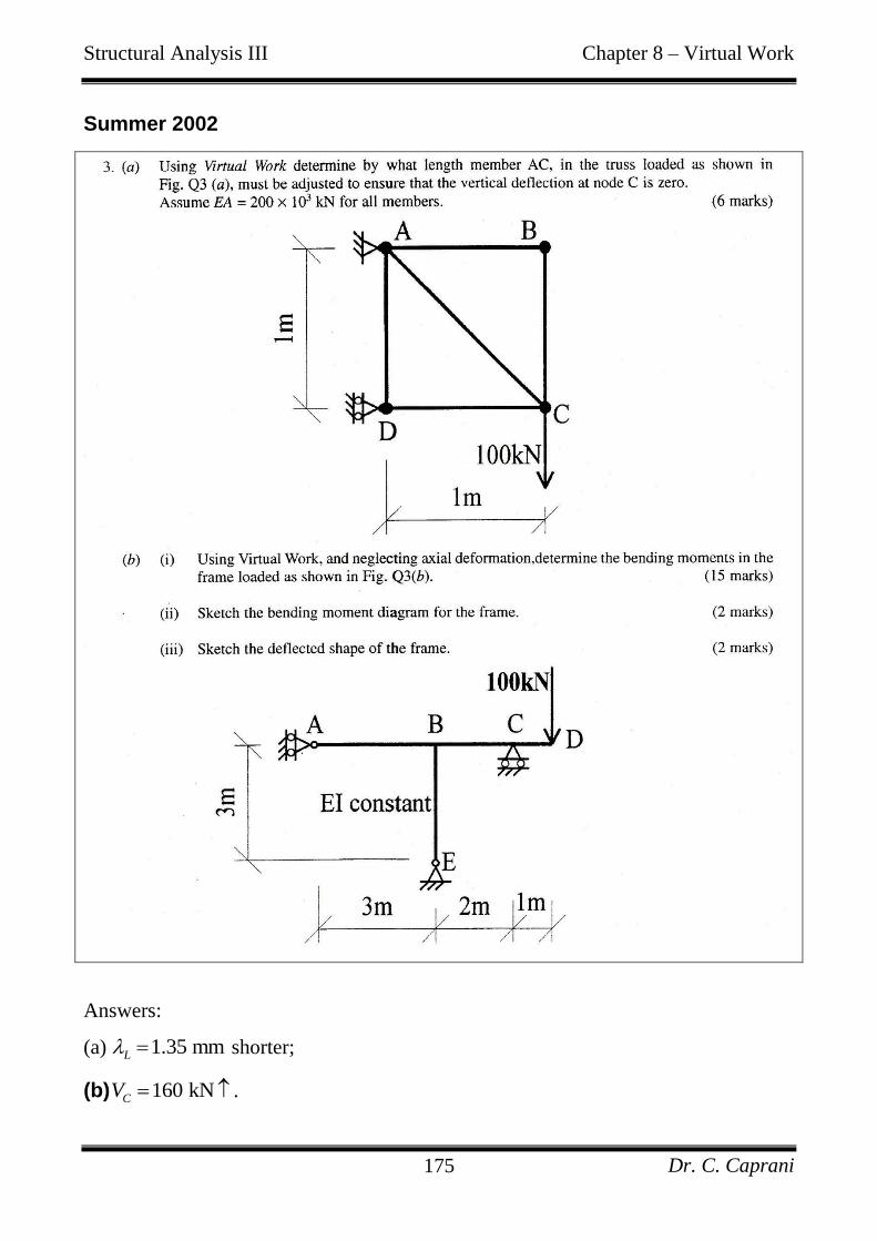
Structural Analysis III Chapter 8 – Virtual Work
Dr. C. Caprani 175
Summer 2002
Answers:
(a) 1.35 mmL shorter;
(b) 160 kNCV .
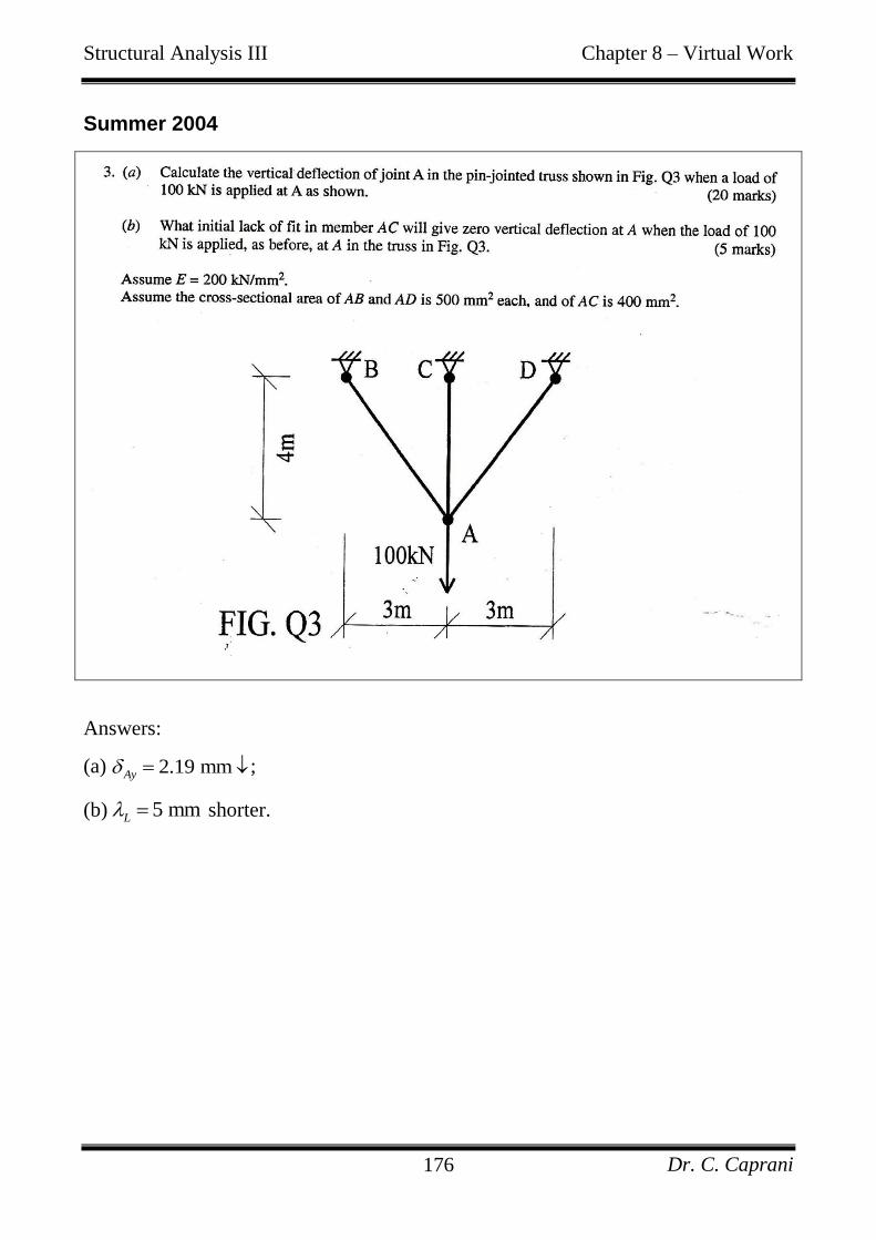
Structural Analysis III Chapter 8 – Virtual Work
Dr. C. Caprani 176
Summer 2004
Answers:
(a) 2.19 mmAy ;
(b) 5 mmL shorter.

Structural Analysis III Chapter 8 – Virtual Work
Dr. C. Caprani 177
Summer 2007
Using Virtual Work:
(i) For the frame in Fig. Q3(a), determine the horizontal deflection of joint C;
(ii) Draw the bending moment diagram for the frame in Fig. Q3(b);
(iii) Determine the horizontal deflection of joint C for the frame in Fig. Q3(b).
Note:
You may neglect axial effects in the members.
Take 3 236 10 kNmEI for all members.
Answers:
(a) 84.6 mmCx ;
(b) 75.8 kNDH ;
(c) 19.02 mmCx .
FIG. Q3(a)
FIG. Q3(b)

Structural Analysis III Chapter 8 – Virtual Work
Dr. C. Caprani 178
Semester 2, 2008
For the frame shown in Fig. Q2, using Virtual Work:
(a) Determine the following:
reactions;
bending moment diagram.
(b) After construction, it is found that the support at C is not rigid but a spring support of stiffness 2000 3 kN/mk .
Taking this into account, determine the following:
vertical displacement of joint C;
bending moment diagram.
(40 marks)
Note:
You may neglect axial effects in the members.
Take 3 236 10 kNmEI for all members.
Answers:
(a) 35.63 kNCV ;
(b) 45 mmCy .
FIG. Q2

Structural Analysis III Chapter 8 – Virtual Work
Dr. C. Caprani 179
Semester 2, 2009
QUESTION 2
Using Virtual Work, for the frame shown in Fig. Q2, do the following:
(i) Determine the reactions;
(ii) Draw the bending moment diagram;
(iii) Draw the deflected shape of the structure;
(iv) Determine the horizontal deflection of joint D.
(25 marks)
Note:
Take 2200 kN/mmE and 7 445 10 mmI for all members.
Answers:
(a) 225 kNBV ;
(b) 81.25 mmDx .
FIG. Q2

Structural Analysis III Chapter 8 – Virtual Work
Dr. C. Caprani 180
Semester 2, 2009
QUESTION 3
For the structure shown in Fig. Q2, due to an error on site, it is required to make the moment at support A zero. This is
to be done by the introduction of a spring support at B, in place of the roller support, as shown in Fig. Q3. Using Virtual
Work:
(i) Determine the spring stiffness required so that the moment at A is zero.
(ii) Drawn the revised bending moment diagram;
(iii) Draw the revised deflected shape of the structure;
(iv) Determine the vertical deflection of the structure at B.
(25 marks)
Note:
Take 2200 kN/mmE and 7 445 10 mmI for all members.
You may use any relevant results from your workings for Q2, but in doing so acknowledge their source.
Answers:
(a) 320 10 kN/mk ;
(b) 7.5 mmBy .
FIG. Q3

Structural Analysis III Chapter 8 – Virtual Work
Dr. C. Caprani 181
Semester 2, 2010
QUESTION 2
Using Virtual Work, for the continuous beam shown in Fig. Q2, do the following:
(i) Draw the bending moment diagram, noting all important values;
(ii) Draw the deflected shape of the structure;
(iii) Determine the deflection at E.
(25 marks)
Note:
Take 2200 kN/mmE and 7 420 10 mmI for all members;
The following expression may be of assistance:
0 1 1 1 2 1
1
0 2 1 2 2 22
0
0
M M M M M M
EI EI EI
M M M M M M
EI EI EI
Answers:
(a) 174.5 kNm; 97.6 kNmB CM M ;
(b) 16.9 mmEy .
FIG. Q2

Structural Analysis III Chapter 8 – Virtual Work
Dr. C. Caprani 182
Semester 2, 2011
QUESTION 3
Using Virtual Work, for the truss shown in Fig. Q3, do the following:
(i) Determine the member forces;
(ii) Draw the member forces using conventional arrow notation;
(v) Draw the deflected shape of the structure;
(iii) Determine the vertical deflection of joint E.
(25 marks)
Note:
Take 2200 kN/mmE ;
21500 mmA for members BC, BF, CE, and EF;
21500 2 mmA for members BE and CF;
22000 mmA for members AF and DE;
22500 mmA for members AB and CD.
Answers:
(a) 15 2 kNBEF compression;
(b) 4.25 mmEy .
FIG. Q3

Structural Analysis III Chapter 8 – Virtual Work
Dr. C. Caprani 183
8.8 References
Charlton, T.M., Analysis of Statically Indeterminate Frameworks, Longmans,
1961.
Charlton, T.M., Energy Principles in Theory of Structures, Oxford University
Press, 1973.
Coates, R.C., Coutie, M.G. and Kong, F.K., Structural Analysis, Chapman and
Hall, 1987.
Davies, G.A.O., Virtual Work in Structural Analysis, John Wiley & Sons, 1982.
Dym, C.L., Structural Modeling and Analysis, Cambridge University Press, 2005.
Gregory, M.S., Introduction to Extremum Principles, Butterworths, London, 1969.
Guarracino, F. and Walker, A., Energy Methods in Structural Mechanics, Thomas
Telford, 1999.
Heyman, J., Beams and Framed Structures, 2nd Edn., Pergamon Press, 1974.
Kong, F.K., Prentis, J.M. and Charlton, T.M., ‘Principle of virtual work for a
general deformable body – a simple proof’, The Structural Engineer, Vol. 61A,
No. 6, 1983.
Neal, B.G., Structural Theorems and their Applications, Pergamon Press, 1964.
Thompson, F. and Haywood, G.G., Structural Analysis Using Virtual Work,
Chapman and Hall, 1986.
Rajasekaran, S. and Sankarasubramanian, G., Computational Structural
Mechanics, Prentis Hall of India, New Delhi, 2001.
Richards, T.H., Energy methods in Stress Analysis, Ellis Horwood, 1977.
Wallerstein, D.V. , A Variational Approach to Structural Analysis, Wiley, 2001.

Structural Analysis III Chapter 8 – Virtual Work
Dr. C. Caprani 184
8.9 Appendix – Volume Integrals
1
3jkl
1
6jkl 1 2
12
6j j kl
1
2jkl
1
6jkl
1
3jkl 1 2
12
6j j kl
1
2jkl
1 2
12
6j k k l 1 2
12
6j k k l
1 1 2
2 1 2
12
6
2
j k k
j k k l
1 2
1
2j k k l
1
2jkl
1
2jkl 1 2
1
2j j kl jkl
1
6jk l a
1
6jk l b
1
2
1
6j l b
j l a k
1
2jkl
5
12jkl
1
4jkl 1 2
13 5
12j j kl
2
3jkl
1
4jkl
5
12jkl 1 2
15 3
12j j kl
2
3jkl
1
4jkl
1
12jkl 1 2
13
12j j kl
1
3jkl
1
12jkl
1
4jkl 1 2
13
12j j kl
1
3jkl
1
3jkl
1
3jkl 1 2
1
3j j kl
2
3jkl
1 2
1 2
1 2
1 2
1 2
1 2
1 2
1 2
1 2
1 2
1 2
1 2
1 2
1 2
1 2
1 2
1 2
1 2
1 2
1 2
1 2
1 2
1 2
1 2
1 2
1 2