Mechanical behavior of metal loss in heat affected zone of welded joints in low carbon steel pipes.

M. J. Fernández C.1, J. L. González V.2, G. Jarvio C.3, J. A. Villalobos G.1

1 Tuxtepec Institute of Technology ITT

2 National Polytechnic Institute IPN 3 Nuclear Research National Institute ININ

Abstract The mechanical behavior of metal loss, localized in the heat affected zone of welded joints in low carbon steel pipes, was analyzed by mean of the finite element method, considering the non linear material behavior (plasticity). The numerical experimentation was done for metal losses of different length and depth, considering the kinematic hardening rule and pressurizing internally the pipe monotonically until the ultimate tensile strength was reached, to determine the limit load than it can support before the failure. Furthermore, hydrostatic testing with measuring of the deformation using strain gages placed in different locations of interest was realized, to verify the results obtained by mean of numerical experimentation, founding that is possible to operate a pipe with metal loss than generate stress near to yield stress, without to affect its global operation. 1. Introduction. The metal loss located in the heat affected zone of pipes subject to internal pressure is a form of damage that causes a decrease in its mechanical strength. This defect may occur as a simple metal loss, metal loss multiple or generalized loss of thickness, and its effect on the mechanical strength depends primarily on its size, diameter and thickness of the pipe, as well as material properties. Analytical methods for evaluation of metal loss in pipes with internal pressure are based on the stress determination in the area of damage, through established procedures such as ANSI B31G or the recommended practice API RP 579, comparing the solution with the strength of the material to determine if the component is fit to continue operating safely. These methodologies, based on codes or recommended practices limit the assessment of metal loss located near welds, considering imminent rejection. However, it has been in hydrostatic test of pipes containing metal losses, have endured greater pressure loads to the established limit, located both in the shell and in the heat affected zone (HAZ). This led to detailed analysis by FEM considering the kinematic hardening of the material to obtain a comparable response to hydrostatic test results, determining the remaining strength of the pipe.

6th Pipeline Technology Conference 2011

2. Development 2.1 Non linear behavior of material A cylindrical vessel subjected to internal pressure regulation operates stress levels below the yield point of material. However, at present a metal loss, the level of stress may eventually exceed the material yield stress, bringing the affected section to operate in the elastic plastic regime, where it is necessary to use the theory of plasticity to explain the nonlinear behavior of material. The incremental plasticity theory provides a mathematical relationship that characterizes the stress and strain increments to represent the behavior of a material in the plastic range. There are 3 basic components of incremental plasticity theory [1] called yield criterion, flow rule and hardening rule. The elastic plastic laws are path-dependent and dissipative. Much of the work consumed in plastically deforming the material is irreversibly converted into other forms of energy, particularly heat. The stress depends on the complete history of deformation and can not be written as a simple function of the strain tested, can be specified as a relationship between estimated values of stress and strain. 2.1.1 Yield criterion. When a material reaches its yield stress in uniaxial tension, it begins to deform plastically. In practical situations, it is common that the material is under a combined stress state and plastic deformation can occur at different stress than yield stress in uniaxial tension. The determination of yield criteria under a combined statement of stress must be an invariant, and that does not depend on the orientation, eliminating the hydrostatic stress because not to cause deformation. [2] The evaluation criterion was the von Mises expressed by:

231

2

32

2

212

1 y

The yielding occurs when the equivalent stress exceeds the yield stress of material:

ye

2.1.2 Flow rule. It prescribes the direction of plastic deformation when the yield point occurs. Defined as the individual components of plastic deformation (εx

pl, εypl, εz

pl) developed in yielding. Flow equations, which are derived from the yield criterion, which typically involve plastic deformations develop in a direction normal to the yield surface. 2.1.3 Hardening rule. It describes as the initial yield point criterion change with the progressive plastic deformation. The hardening rule describes how the yield surface is changed during plastic flow. Determined when the material will yield again if the load is maintained or if the load is reversed. The yield surface varies at each stage of plastic deformation, adopting an alternative model for strain hardening.

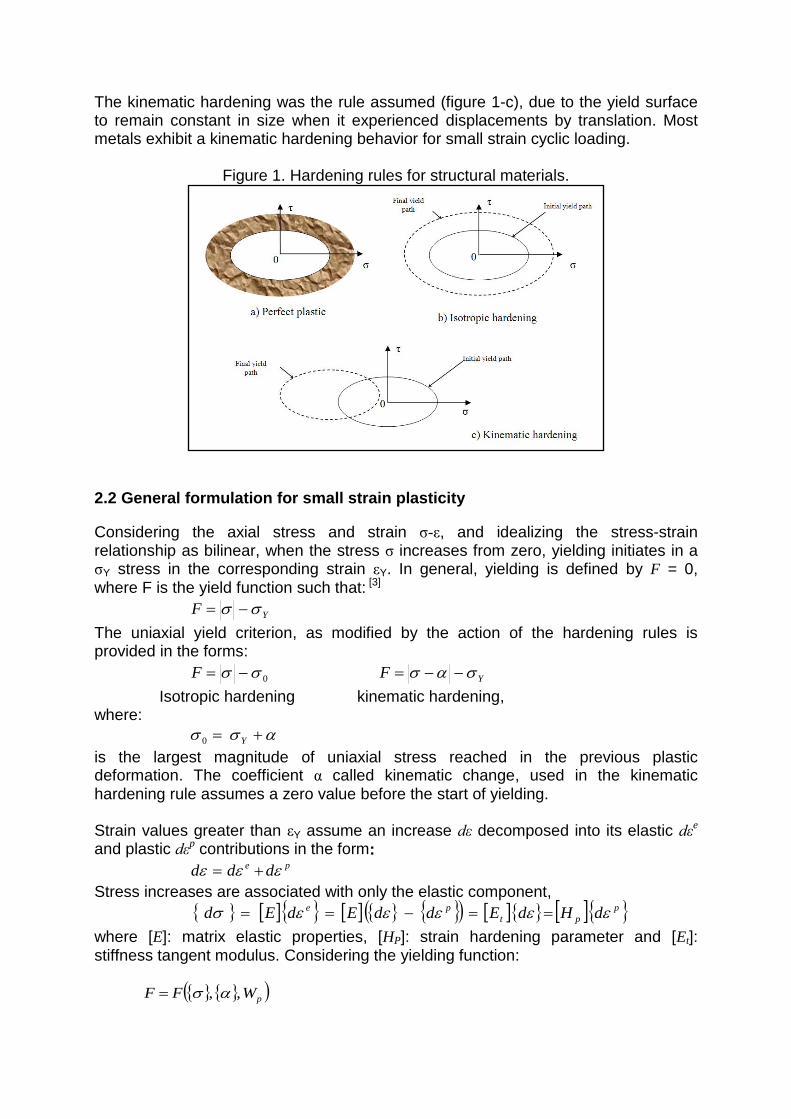
The kinematic hardening was the rule assumed (figure 1-c), due to the yield surface to remain constant in size when it experienced displacements by translation. Most metals exhibit a kinematic hardening behavior for small strain cyclic loading.

Figure 1. Hardening rules for structural materials.

2.2 General formulation for small strain plasticity

Considering the axial stress and strain σ-ε, and idealizing the stress-strain relationship as bilinear, when the stress σ increases from zero, yielding initiates in a σY stress in the corresponding strain εY. In general, yielding is defined by F = 0, where F is the yield function such that: [3]

YF

The uniaxial yield criterion, as modified by the action of the hardening rules is provided in the forms:

0 F YF

Isotropic hardening kinematic hardening, where:

Y0

is the largest magnitude of uniaxial stress reached in the previous plastic deformation. The coefficient α called kinematic change, used in the kinematic hardening rule assumes a zero value before the start of yielding. Strain values greater than εY assume an increase dε decomposed into its elastic dε

e

and plastic dεp contributions in the form:

pe ddd

Stress increases are associated with only the elastic component,

p

pt

pe dHdEddEdEd

where [E]: matrix elastic properties, [HP]: strain hardening parameter and [Et]: stiffness tangent modulus. Considering the yielding function: pWFF ,,

pW,

dQ

d p

dd ,

Where values of count for the hardening, describing how a yield surface is altered in the multidimensional stress space, for changes in the size or location in response to plastic deformation. The flow rule is defined in terms of a function Q, called the plastic potential. With a scalar dλ called plastic multiplier, increments in plastic deformation are given by: .

Modeling considering a kinematic hardening, it is represented by the vector ,

which considers displacement of the yield surface in the vector space, represented as:

pdC ,

expression obtained from the integration of:

pdCd ,

2

1

2

1

2

1111

3

2PHC ,

being HP the plastic modulus of the material. For an increase in plastic deformation, dF = 0, is obtained from the yield function:

0

d

Fd

FTT

.

Replacing the plastic deformation increases in the equation for the increase of stress associated with the elastic component, so as the kinematic hardening vector is obtained:

dQ

CddQ

dEd

, .

Replacing the expressions for in the penultimate equation and solving the resulting equation for the plastic multiplier dλ is obtained:

dPd , where P is the row matrix:

QC

FQE

F

EF

PTT

T

.

Finally, from the equations for dd , and d is obtained:

dEd ep ,

P

QIEEep

.

Where I is a unitary matrix. The elastic plastic matrix epE can be considered a

generalized form of the tangent modulus Et. 2.3 Multilinear kinematic hardening Decomposing σ-ε curve of the material in various stages or steps of loading, limiting each load step with a specified minimum strength, defines a multi linearity of σ-ε curve that presents the kinematic hardening shown in figure 2, for each plasticity conditions. The portion of total load for each sub-step and its corresponding minimal

kk ,

svN

resistance define the increased plastic deformation, assuming that each sub-step is subjected to the total strain. The individual increments of plastic strain, whereas a weighting factor determining the total or apparent increase in the plastic deformation. The plastic deformation is updated and the elastic deformation is calculated.

1

1

3

21

K

iTK

TK Wi

EV

E

EEWk

For : Wk is a weighting factor to sub-step k, evaluated sequentially; TkE is the

modulus of elasticity of the curve segments σ-ε, and

iW sum of weighting factors prior assessment of sub-step load.

Figure. 2. Uniaxial behavior for multi linear kinematic hardening.

The minimum stress for each sub-load step is given by:

))21(3()1(2

1kvkE

vyk

where represent increases in stress-strain curve. The number of load steps is the number of interruptions of the curve. The increase in plastic deformation for each sub-step is analyzed and using the von Mises yield criterion compared to the ratio of the flow rule. The increase in plastic deformation for all sub-steps is the sum of the increments of plastic deformation, expressed as:

Nsv

i

Pl

i

Pl Wi1

where: : number of sub-steps.

2.4 Experimental work 2.4.1 Numerical experimentation by mean of FEM 20 models were generated in three dimensions considering the geometry and dimensions of the pipe (table 1), with metal loss located in the HAZ, oriented in the longitudinal direction on the pipe diameter and depth increments (%d/t) of 10, 20, 33, 50 and 80%.

Table 1. Dimensions of pipe and metal loss for analysis by FEM.

Longitudinal metal loss

cases D t Lm d %d/t b

mm mm mm mm

mm

1 609.6 10.439 25.4 1.0439 10 0.7700

2 609.6 10.439 101.6 1.0439 10 0.7700

3 609.6 10.439 177.8 1.0439 10 0.7700

4 609.6 10.439 254 1.0439 10 0.7700

5 609.6 10.439 25.4 2.0879 20 0.7700

6 609.6 10.439 101.6 2.0879 20 0.7700

7 609.6 10.439 177.8 2.0879 20 0.7700

8 609.6 10.439 254 2.0879 20 0.7700

9 609.6 10.439 25.4 3.4450 33 0.7700

10 609.6 10.439 101.6 3.4450 33 0.7700

11 609.6 10.439 177.8 3.4450 33 0.7700

12 609.6 10.439 254 3.4450 33 0.7700

13 609.6 10.439 25.4 5.2197 50 0.7700

14 609.6 10.439 101.6 5.2197 50 0.7700

15 609.6 10.439 177.8 5.2197 50 0.7700

16 609.6 10.439 254 5.2197 50 0.7700

17 609.6 10.439 25.4 8.3515 80 0.7700

18 609.6 10.439 101.6 8.3515 80 0.7700

19 609.6 10.439 177.8 8.3515 80 0.7700

20 609.6 10.439 254 8.3515 80 0.7700

The geometry of metal losses considered in this work is an approach that applies the parameters evaluated in a real scale test, in order to determine the remaining strength of steel pipe API 5LX52 containing defects referrals. The parameters are shown in Figures 3 and 4, where:

D: pipe diameter t: wall thickness Lm: longitudinal metal loss d: depth of the metal loss b: width of the metal loss

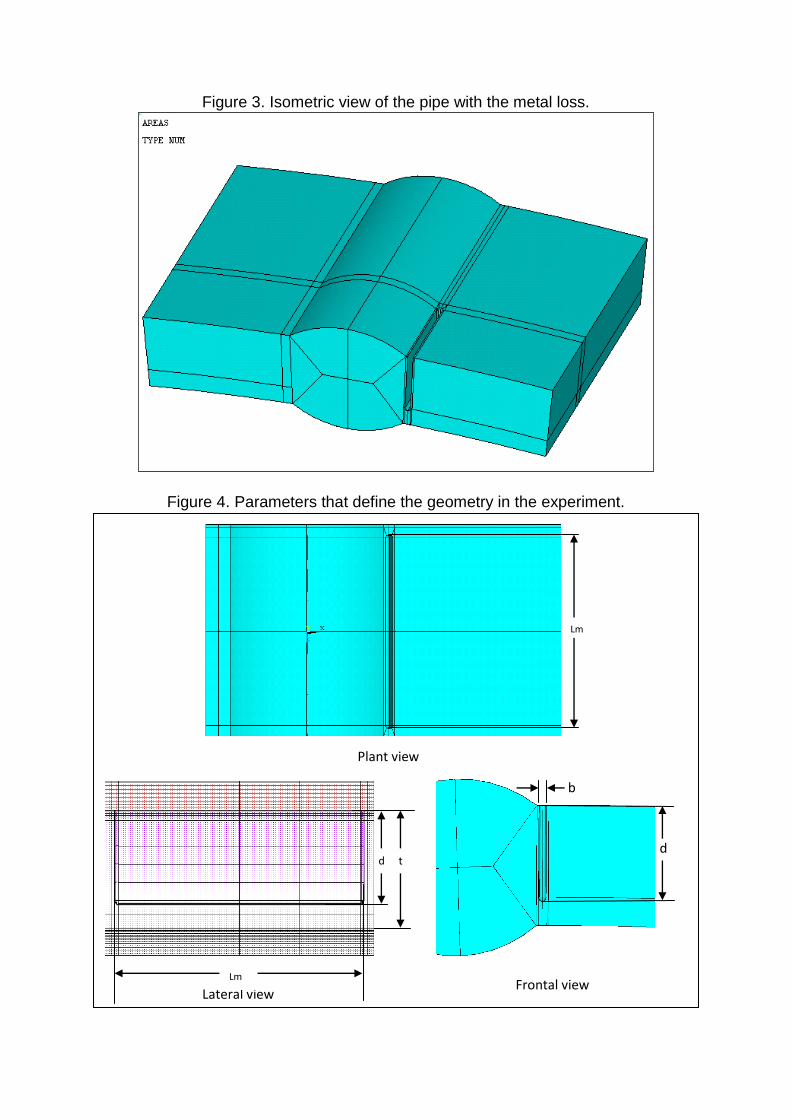
Figure 3. Isometric view of the pipe with the metal loss.

Figure 4. Parameters that define the geometry in the experiment.

Lateral view Frontal view

Lm

m

Plant view

d

b

t d

Lm

The FEM analysis considered only one half of the model due to the symmetry of the system, allowing apply more computational resources in the refined finite element mesh in the area of the defect. A finite element model for the case% d/t=80, Lm=25.4 mm shown in figure 5.

Figure 5. FEM mesh showing one half model.

The implementation of the models used solid isoparametric elements 45 first order, with eight nodes in each element and capacity in elasticity, plasticity, large deformation and stiffness stress for all cases. The mechanical properties considered in the simulation correspond to the values obtained in tensile test in regions HAZ-PM-WM, of sections of pipe removed from service for a low carbon steel grade API 5LX52 (figure 6).

Figure 6. True stress-strain diagram for base metal, HAZ and Weld metal.

0

100

200

300

400

500

600

700

0,0000 0,0200 0,0400 0,0600 0,0800 0,1000 0,1200 0,1400 0,1600

tru

e s

tre

ss

, M

Pa

logarithmic strain, mm/mm

True stress-strain diagram

base metal

weld metal

heat affected zone

The elastic plastic behavior of the material required the implementation of a nonlinear analysis, to solve the FEM models to define the mechanical behavior when considering the action of internal pressure load. In a nonlinear analysis solution can not be predicted directly with a group of linear equations. A non-linear structure can be analyzed through a series of iterative linear approximations with corrections. The ANSYS finite element program uses an iterative process called the method of Newton-Raphson, where each iteration is known as an iteration of equilibrium. [4] Each iteration is a separate step through the solution of the equation, and a full iterative analysis is for an increase in load. The Newton-Raphson method iterates until a solution (figure 7) by the equation

nrT FFuK

where:

:TK tangent stiffness matrix

:u increase of displacement

:F external loads vector

:nrF internal loads vector

Figure 7. Iterative process of solution by the Newton-Raphson method.

The solution of nonlinear finite element models for each of the case studies was carried out considering a sequence of increases in internal pressure load. Initiated load increases from zero, reaching the internal pressure than generated yield stress σy, through the flow stress to reach the ultimate tensile strength. This allowed to know the pressure loads that can lead eventually to a failure condition in a pipe with a metal loss in the region of the HAZ.

u

F

u1

Fnr

1

KT

1

1

2

3

4 5

2.4.2 Hydrostatic test in a pipe containing metal loss. The hydrostatic test is performed to evaluate the real behavior of the pipe, considering the presence of metal loss in the HAZ, and also allows verification of the results obtained by numerical simulation. The pipe was tested as a pressure vessel, to be kept sealed with end caps and subjected to pressure load through the entry of water pumping equipment (water was used neutral and free of suspended solids). The test was conducted at a temperature of 20ºC, using a calibrated pressure gauge connected to the pipe, with water as incompressible fluid whose behavior did not generate pressure increase risk. [5] The hydrostatic test pressure for the pipe was determined by a standard as sealed hydrostatic test, depending on the system operating pressure and maximum pressure emergency. Although hydrostatic pressure is usually 1.5 times the normal operating pressure, which in no case exceed 90% of the yield stress limit for the material [6], our experimental pressure values considered to lead to pipe until failure, with a number of defects oriented in the HAZ. The deformation produced in the pipe during the hydrostatic test was evaluated by electrical strain gages, capable of measuring in the elastic plastic range. The surface preparation for bonding of the strain gages (figure 8) was developed according to guidelines set by the manufacturer. [7,8] A conditioned trench was prepared for the hydrotest, where the pipe instrumented with strain gages was hosted, which were connected to a strain indicator (figure 9).

Figure 8. Surface preparation and bonding of strain gages.

Figure 9. Instrumented pipe and strain indicator.

During the course of the hydrotest, allowed the free flow of water throughout the vessel, to fill it completely. It opened the vent valve to remove air from the pipe, with the gradual closure of the same water leaving no bubbles. A hydraulic pump slowly increased the pressure in the vessel, with increments of 10 kg/cm2 to reach the design pressure. In each increment of pressure is stopped the operation of the pump, waiting for a time of 10 minutes to stabilize, proceeding with the process of reading strain for each strain gage. Design pressure is reached, the pressure increased again in periods of 10 minutes, through values than generated yield stress, flow stress, ultimate tensile strength in tension and finally up to the failure. It was verified that at each step of loading pressure don´t exist leaks. 3 Results FEM numerical simulation revealed that the magnitude of the maximum pressure to achieve the allowable yield stress decreases with increasing defect length or depth. As the defect is deeper, the estimation of internal pressure load becomes more significant with increasing the length Lm. Figure 10 shows this behavior, reaching a considerable involvement as they increase the size of Lm in metal loss with d/t= 80%.

Figure 10. Internal pressure load and the geometry analyzed.

The stress generated according to the von Mises criterion was reached at a lower pressure load, when the metal loss was deeper, to remain constant in length Lm. Figure 11 shows this behavior, considering a length of Lm = 177.80 mm, whose verification was possible because there is the same case between the two methodologies.

0,00

0,01

0,01

0,02

0,02

0,03

0,03

0,04

0 2 4 6 8 10 12

load-geometry diagram

d/t=10%

d/t=20%

d/t=33%

d/t=50%

d/t=80%

Figure 11. Internal pressure load and von Mises stress.

Also, in developing the hydrostatic test, the values of the strain in defects of different sizes was evaluated, which are shown in Table 2. An stress estimate calculated from the maximum strain recorded by extensometer is shown in this table, comparing with the result obtained by the numerical experiment by FEM. Difference between the solution obtained by both methods showed a maximum value of 5.39% for Lm=177.8 mm with d/t=20%. This difference can be assumed to be negligible since the average variation between the two solutions was 0.91%.

Table 2. strain and stress obtained from hydrotest data.

Strain gage

Lm d/t Max strain, Hydrotest

Stress obtained by max. strain

Stress, FEM

mm % mm/mm MPa MPa

1 254.00 10 0.001058 219.006 216.991

2 101.60 10 0.001838 380.466 376.562

3 177.80 50 0.002968 614.376 613.169

4 177.80 33 0.001503 311.121 306.852

5 25.40 10 0.001453 300.771 298.054

6 177.80 20 0.001437 297.459 281.418

7 101.60 20 0.001447 299.529 309.685

It is important to say than the final failure in the pipe subjected to internal pressure load in the hydrotest occurs in a region different to the metal loss location in the HAZ (figure 12). This shown than is possible to consider a FEM solution as a reliable evaluation method, because to permit determine internal pressure load than can lead to the pipe to a stress state that reflects its real mechanical behavior.

0

100

200

300

400

500

600

700

0 5 10 15 20 25

vo

n M

ise

s s

tres

s, M

Pa

internal pressure load, MPa

stress-load diagram, Lm=177.80 mm

10%d/t20%d/t33%d/t50%d/t80%d/t

The assessment should include factors to consider possible contingencies that modify the stress-strain behavior of the pipe with metal loss, to ensure safe operation of the same, without affecting people, environment and property.

Figure 12. Final failure in the pipe in defect output of the HAZ.

4 Conclusions For all cases examined, the presence of an external metal loss in the HAZ longitudinally oriented, of a pipe subjected to internal pressure limits their ability to withstand pressure load. However, it is possible to work with pressure values that generate locally yield stress without affecting the operation of the pipe. Additionally, a limit value to pressurize the pipe corresponds to the load pressure generated by a local state of stress in the same magnitude as the material flow stress. To match this condition, the pipe could withstand load eventually increased pressure to finally bring it to achieve the ultimate tensile strength, although this condition is not recommended because it is close to the plastic collapse. Reduce as far as possible the pressure load to levels to produce locally yield stress as permissible condition, and pressure load to produce locally flow stress as a condition acceptable limit. It is possible than loads greater than these values may eventually compromise the integrity of the pipe. 5 References [1] T. Belytschko, W. Kam L., B. Moran, “Non Linear Finite Elements for Continua

and Structures”, Editorial: John Wiley, 2001. [2] A. S. Khan, S. Huang, “Continuum Theory of Plasticity”, Editorial: John Wiley &

Sons Inc, 1995. [3] R. D. Cook, D. S. Malkus, M. E. Plesha, R. J. Witt, “Concepts and Applications

of Finite Element Analysis”, Editorial: John Wiley & Sons Inc., Fourth Edition, 2002.

[4] ANSYS Release 11. Structural Analysis Guide. ANSYS, Inc. is UL registered ISO 9001:2000 Company, November 2004.

[5] NORMA OFICIAL MEXICANA NOM-020-STPS-2002. Pressure vessels subject to internal pressure and boilers in security conditions performance.

[6] NORMA OFICIAL MEXICANA NOM-012/3-SEDG-2003. Pressure vessels subject to internal pressure to storage LP Gas.

[7] Vishay Measurements Group, “Catalog 500, Precision Strain Gages”, March 1996.

[8] Vishay Measurements Group, M-Line Strain Gages Accessories, Catalog A-110-9, 1994.

6 Thanks The author thanks to the GAID-IPN-México the facilities to carry out the hydrotest in the low carbon steel pipe containing the metal loss.