Lectures on Dynamic Systems and

Control

Mohammed Dahleh Munther A. Dahleh George Verghese

Department of Electrical Engineering and Computer Science

Massachuasetts Institute of Technology1

1�c

Chapter 28

Stabilization: State Feedback

28.1 Introduction: Stabilization

One reason feedback control systems are designed is to stabilize systems that may be unstable. Al-though our earlier results show that a reachable but unstable system can have its state controlled by

appropriate choice of control input, these results were obtained under some critical assumptions:

� the control must be unrestricted (as our reachability results assumed the control could be chosen

freely)�

� the system must be accurately described (i.e. we must have an accurate model of it)�

� the initial state must be accurately known.

The trouble with unstable systems is that they are unforgiving when assumptions such as the above do

not hold. Even if the �rst assumption above is assumed to hold, there will undoubtedly be modeling

errors, such as improperly modeled dynamics or incompletely modeled disturbances (thus violating

the second assumption). And even if we assume that the dynamics are accurately modeled, the initial

state of the system is unlikely to be known precisely (violating the third assumption). It is thus clear

that we need ongoing feedback of information about the state of the system, in order to have a hope

of stabilizing an unstable system. Feedback can also improve the performance of a stable system (or,

if the feedback is badly chosen, it can degrade the performance and possibly cause instability!). We

shall come to understand these issues better over the remaining lectures.

How, then, can we design feedback controllers that stabilize a given system (or plant | the word

used to describe the system that we are interested in controlling) � To answer this, we have to address

the issues of what kind of feedback variables are available for our controller. There are, in general, two

types of feedback:

� state feedback

� output feedback.

With state feedback, all of the state variables (e.g., x) of a system are available for use by the controller,

whereas with output feedback, a set of output variables (e.g., y � Cx+Du) related to the state variables

are available. The state feedback problem is easier than the output feedback one, and richer in the

sense that we can do more with control.

In the remainder of this chapter, we examine eigenvalue placement by state feedback. All our

discussion here will be for the case of a known LTI plant. The issue of uncertainty and unmodeled

dynamics should be dealt with as discussed in previous chapters� namely, by imposing a norm constraint

on an appropriate closed loop transfer function. Our development in this lecture will use the notation

of CT systems | but there is no essential di�erence for the DT case.

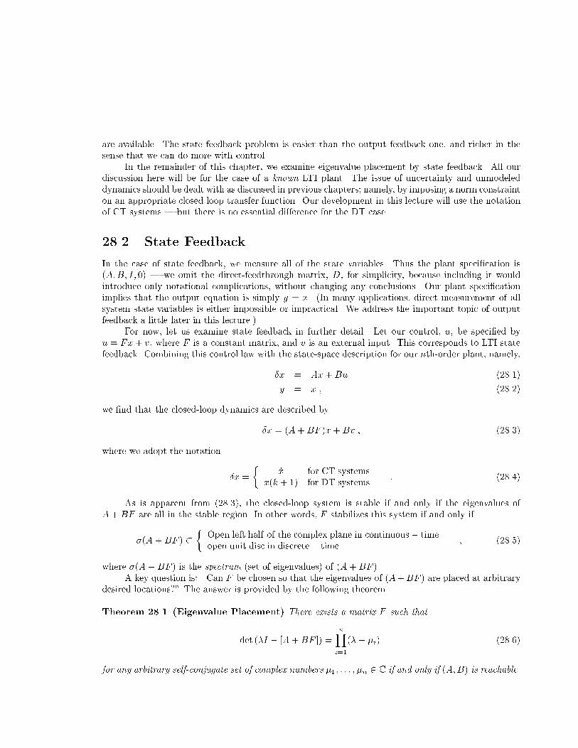
28.2 State Feedback

In the case of state feedback, we measure all of the state variables. Thus the plant speci�cation is

(A� B� I� 0) | we omit the direct-feedthrough matrix, D, for simplicity, because including it would

introduce only notational complications, without changing any conclusions. Our plant speci�cation

implies that the output equation is simply y � x. (In many applications, direct measurement of all

system state variables is either impossible or impractical. We address the important topic of output

feedback a little later in this lecture.)

For now, let us examine state feedback in further detail. Let our control, u, be speci�ed by

u � Fx + v, where F is a constant matrix, and v is an external input. This corresponds to LTI state

feedback. Combining this control law with the state-space description for our nth-order plant, namely,

�x � Ax + Bu (28.1)

y � x � (28.2)

we �nd that the closed-loop dynamics are described by

�x � (A + BF )x + Bv � (28.3)

where we adopt the notation �

x_ for CT systems

�x � : (28.4)x(k + 1) for DT systems

As is apparent from (28.3), the closed-loop system is stable if and only if the eigenvalues of

A + BF are all in the stable region. In other words, F stabilizes this system if and only if �

�(A + BF ) �

Open left half of the complex plane in continuous ; time

� (28.5)open unit disc in discrete ; time

where �(A + BF ) is the spectrum (set of eigenvalues) of (A + BF ).

A key question is: \Can F be chosen so that the eigenvalues of (A + BF ) are placed at arbitrary

desired locations�" The answer is provided by the following theorem.

Theorem 28.1 (Eigenvalue Placement) There exists a matrix F such that

nY

det (�I ; [A + B F ]) � (� ; �i) (28.6)

i�1

for any arbitrary self-conjugate set of complex numbers �1� : : : � �n

2 C if and only if (A� B) is reachable.

Proof. To prove that reachability is necessary, suppose that �i

2 �(A) is an unreachable mode. Let

wiT be the left eigenvector of A associated with �i. It follows from the modal reachability test that

wiT A � �iwi

T and wiT B � 0. Therefore,

wiT (A + BF ) � wi

T A + (wiT B)F

� wiT A + 0

� �iwiT : (28.7)

Equation (28.7) implies that �i

is an eigenvalue of (A + BF ) for any F . Thus, if �i

is an unreachable

mode of the plant, then there exists no state feedback matrix F that can move it.

We shall prove su�ciency for the single-input (B � b) case only. (The easiest proof for the multi-input case is, as in the single-input case below, based on a canonical form for reachable multi-input

systems, which we have not examined in any detail, and this is why we omit the multi-input proof.)

Since (A� b) is reachable, there exists a similarity transformation x � Tz such that T

;1AT and T

;1b

have the controller canonical form 32 ;�1

;�2

� � � ;�n

1 0 � � � 0

. .

~A � T

;1AT �

6664

7775

(28.8)

.

1 0 32

1

0

. .

6664

7775

~b � T

;1b � : (28.9)

.

0

Recall that the coe�cients �i

in the matrix A~ de�ne the characteristic polynomial of A~ and A:

�(�) � �n + �1�n;1 + � � � + �n

(28.10)

Let Yn(� ; �i) � �n + �d

1

�n;1 + � � � + �d � �d(�) : (28.11)n

i�1

~ ~If u � Fz with F being the row vector ��

F~ � f~

1

� � � f~

n

then 32 ;�1

+ f~

1

;�2

+ f~

2

� � � ;�n

+ f~

n

1 0 � � � 0

. .

6664

7775

A~ + ~bF~ � : (28.12)

.

1 0

~It is evident that we simply have to choose fi

� ;�di

+ �i

for i � 1� : : : � n to get the desired closed-loop

characteristic polynomial �d(�).

We have thus been able to place the eigenvalues in the desired locations. Now, using the similarity

transformation and F~, we must �nd F so that A + bF has the same eigenvalues. Since u � F~ z and

~T

;1 ~ x � Tz, u � F x. Thus we should de�ne F � FT

;1 . (Verify that A + bF has the same eigenvalues

as A~ + ~bF~.) This completes the proof.

The calculation that was described above of a feedback matrix that places the poles of A + bF at

the roots a speci�ed polynomial �d(s) can be succinctly represented in a simple formula. The matrix

A and A~ have the same characteristic polynomial, �(�), which implies that A~ satis�es

(A~)n � ;�1A~n;1 ; �2A~n;2 ; : : : ; �nI:

Based on the above relation the desired characteristic polynomial satis�es

�d(A~) � A~n + �d1

A~n;1 + �d2

A~n;2 + : : : + �dnI�

� (�1

d ; �1)A~n;1 + (�2

d ; �2)A~n;2 + : : : + (�d ; �n)I: n

We de�ne the unit vectors eTi

, i � 1� 2� : : : � n as ih

T ith positionei

� 0 0 : : : 0 1 0 : : : 0

:

Due to the special structure of the matrix A~ the reader should be able to check that

e

T �d(A~) � (�d

1

; �1)e

T A~n;1 + (�d

2

; �2)e

T A~n;2 + : : : + (�d ; �n)e

T In n n n n

� (�d

1

; �1)eT

1

+ (�d

2

; �2)eT

2

+ : : : + (�d ; �n)eT

n n

� ;F~ :

Recall that the transformation T that transforms a system into reachable form is given by T �

fRn

fRn

;1

Rn

where ��

fRn

� b Ab : : : An;1b �

Rn

��

~b A~~b A~n;1~b� :: : :

The matrix has the following form 32

1 � � : : :

0 1 � : : :

6664

7775

fRn

where � denotes entries that can be di�erent from zero. The feedback matrix F is related to F~ via the

relation F � F~T

;1 which implies that

F � F~T

;1

� ;e

T �d(A~)T

;1

n

� ;e

T �d(T

;1AT )T

;1

n

� ;e

T T

;1�d(A)TT

;1

n

� � (28.13). . . . . . .

. .

0 0 : : : 1

Rn

;1�d(A):;e

T

n

fRn

T

�

TNote that from Equation 28.13 we h � e , w hich results in the following formula, which iave e sn n

fRn

commonly called Ackermann's formula

F � ;e

T Rn

;1�d(A): (28.14)n

Some comments are in order:

1. If (A� B) is not reachable, then the reachable modes, and only these, can be changed by state

feedback.

2. The pair (A� B) is said to be stabilizable if its unreachable modes are all stable, because in this

case, and only in this case, F can be selected to change the location of all unstable modes to

stable locations.

3. Despite what the theorem says we can do, there are good practical reasons why one might temper

the application of the theorem. Trying to make the closed-loop dynamics very fast generally

requires large F , and hence large control e�ort | but in practice there are limits to how much

control can be exercised. Furthermore, unmodeled dynamics could lead to instability if we got

too ambitious with our feedback.

The so-called linear-quadratic regulator or LQR formulation of the controller problem for linear

systems uses an integral-square (i.e. quadratic) cost criterion to pose a compromise between the

desire to bring the state to zero and the desire to limit control e�ort. In the LTI case, and with

the integral extending over an in�nite time interval, the optimal control turns out to be precisely

an LTI state feedback. The solution of the LQR problem for this case enables computation of the

optimal feedback gain matrix F

� (most commonly through the solution of an algebraic Riccati

equation). You are led through some exploration of this on the homework. See also the article

on \Linear Quadratic Regulator Control" by Lublin and Athans in The Control Handbook, W.S.

Levine (Ed.), CRC Press, 1996.

4. State feedback cannot change reachability, but it can a�ect observability | either destroying it

or creating it.

5. State feedback can change the poles of an LTI system, but does not a�ect the zeros (unless the

feedback happens to induce unobservability, in which case what has occurred is that a pole has

been shifted to exactly cancel a zero). Note that, if the open-loop and closed-loop descriptions

are minimal, then their transmission zeros are precisely the values of s where their respective

system matrices drop rank. These system matrices are related by a nonsingular transformation: � � � � � �

sI ; (A + BF ) ;B

�

sI ; A ;B I 0

(28.15)C 0 C 0 F I

Hence the closed-loop and open-loop zeros are identical. (We omit a more detailed discussion of

what happens in the nonminimal case.)

Example 28.1 Inverted Pendulum

A cart of mass M slides on a frictionless surface. The cart is pulled by a force u(t). On the

cart a pendulum of mass m is attached via a frictionless hinge, as shown in Figure 28.1.

The pendulum's center of mass is located at a distance l from either end. The moment

of inertia of the pendulum about its center of mass is denoted by I . The position of the

center of mass of the cart is at a distance s(t) from a reference point. The angle �(t) is

the angle that the pendulum makes with respect to the vertical axis which is assumed to

increase clockwise.

First let us write the equations of motion that result from the free-body diagram of the

cart. The vertical forces P , R and Mg balance out. For the horizontal forces we have the

following equation

Ms�� u ; N: (28.16)

s(t)

theta

l

u(t)

u

P

N

P

N

mg

s+ l sin(theta)

Mg R

Figure 28.1: Inverted Pendulum

From the free-body diagram of the pendulum, the balance of forces in the horizontal

direction gives the equation

d2

m (s + l sin(�)) � N� �

dt2 � �d _m s_ + l cos(�)� � N�

dt� �

m s� ; l sin(�)(�_)2 + l cos(�)�� � N� (28.17)

and the balance of forces in the vertical direction gives the equation

d2

m (l cos(�)) � P ; mg�

dt2 � �d _m ;l sin(�)� � P ; mg�

dt� �

m ;l cos(�)(�_)2 ; l sin(�)�� � P ; mg: (28.18)

Finally by balancing the moments around the center of mass we get the equation

I�� � P l sin(�) ; Nl cos(�): (28.19)

_ _

From equations 28.16, 28.17 we can eliminate the force N to obtain � �

_(M + m)s�+ m l cos(�)�� ; l sin(�)(�)2 � u: (28.20)

Substituting equations 28.17, 28.18 into equation 28.19 gives us � �

I�� � l mg ; ml cos(�)(�_)2 ; ml sin(�)�� sin(�) � �

; l ms� ; ml sin(�)(�_)2 + ml cos(�)�� cos(�):

Simplifying the above expression gives us the equation

(I + ml2)��� mgl sin(�) ; mls�cos(�): (28.21)

The equations that describe the system are 28.20 and 28.21. We can have a further

simpli�cation of the system of equations by removing the term �� from equation 28.20, and

the term �s from equation 28.21. De�ne the constants

Mt

� M + m

I + ml2

L � :

ml

Substituting �� from equation 28.21 into equation 28.20 we get � �

_1 ;

ml

cos(�)2 s�+

ml

g sin(�) cos(�) ;

ml

sin(�)(�)2 �1

u: (28.22)MtL MtL Mt

Mt

Similarly we can substitute �s from equation 28.20 into equation 28.21 to get � �

1 ;

ml

cos(�)2 �� ;

g

sin(�) +

ml

sin(�) cos(�)(�_)2 � ;

1

cos(�)u: (28.23)MtL L MtL MtL

_ .These are nonlinear equations due to the presence of the terms sin(�), cos(�), and (�)2

We can linearize these equations around � � 0 and � � 0, by assuming that �(t) and �(t)

remain small. Recall that for small �

1

sin(�) � � ; �3

6

1

cos(�) � 1 ; �2�

2

and using these relations we can linearize the equations 28.22 and 28.23. The linearized

system of equations take the form � �

ml ml g 1

1 ; s�+ � � u�

MtL MtL L Mt� �

1 ;

ml

�� ;

g� � ;

1

u:

MtL L MtL

Choose the following state variables 2 3

s

x �

664 �s_

775

�

_�

to write a state space model for the invert ed pendulum. Using these state variables the

following state space model can be easily obtained 010 10 101

x1

0 1 0 0 x1

0

�

y � 1 0 0 x�

where the constant � is given by

1

� �

� � :

�

ml1 ; Mt

L

_Intuitively it is clear that the equilibrim point [s � constant� s_ � 0� � � 0� � � 0] is an

unstable equilibrim point. To verify this we compute the eigenvalues of the matrix A by

solving the equation det(�I ; A) � 0. The eigenvalues are

BB@�

BB@

CCA

;�

ml

Mt

L

BB@

CCA

CCA

BB@

CCA

d 00 0 gx2

x2 Mt� + u

00 0 0 1dt

x3

x3

�0 0 �

g 0L;x4

x4 LMt

� �ppTherefore we have two eigenvalues at the j! axis and one eigenvalue in the open right half

of the complex plane, which indicates instability.

Now let us consider the case where M � 2kg, m � :1kg, l � :5m, I � :025kgm2, and of

course g � 9:8m�s2 . Assume that we can directly measure the state variables, s, s_, � and

_�. We want to design a feedback control law u � F x̂+ r to stabilize this system. In order

to do that we will choose a feeback matrix F to place the poles of the closed-loop system

�g �g0 0 ; :

L L

��

at f;1� ;1� ;3� ;3g. Using Ackermann's formula

F � ; 0 0 0 1 Rn

;1�d(A)

where �d(�) � (� + 1)(� + 1)(� + 3)(� + 3) which is the ploynomial whose roots are

the desired new pole locations, and Rn

is the reachability matrix. In speci�c using the

parameters of the problem we have 32

0 0:4878 0 0:1166

;1

2 3

9:0 24:0 ;7:7 ;1:9

;24:9 ;7:7664

664

775

775

��

F � ; 0 0 0 1

0:4878 0 0:1166 0 0 9:0

0 ;0:4878 0 ;4:8971

0 0

0 0 330:6 104:3

;0:4878 ;4:8971 0 0 1047:2 330:6 � �

� 1:8827 5:0204 67:5627 21:4204

The closed-loop system is given by 232 32 323

x1

0 1:0 0 0 x1

0 664

x2

x3

775

�

664

0:9184 2:449 32:7184 10:449

0 0 0 1:0

664

775

x2

x3

775

+

664

775

d

dt

0:4878

0

r

x4

;0:9184 ;2:4490 ;22:9184 ;10:4490 x4

;0:4878

In Figure 28.2 we show the time trajectories of the closed-loop linearized system when the

reference input r(t) is identically zero and the intial angular displacement of the pendulum

Distance From Reference Point Velocity From Reference Point 4 6

3 4

ds/d

t

s 2 2

1 0

0 −2 0 5 10 15 20 0 5 10 15 20

time time

Angle of Pendulum w.r.t Vertical Angular Velocity

thet

a

1 4

3 0.5

d th

eta/

dt

2

0 1

−0.5 0 0 5 10 15 20 0 5 10 15 20

time time

Figure 28.2: Plot of the State Variables of the Closed-Loop Linearized System with r � 0 and

_the Initial Condition s � 0, s_ � 0, � � 1:0, and � � 0

is 1:0 radians. In this simulation the initial conditions on all the other state variables are

zero.

We can also look at the performance of this controller if it is applied to the nonlinear

system. In this case we should simulate the dynamics of the following nonlinear system

of equations 2 3 2 3 2 3

x2

0x1

1 1

Mt

�(x3

)

0

mlg 1 sin(x3) cos(x3) +

ml 1 sin(x3)(x4

)2

�(x3

) Mt

�(x3

)d

dt

664

x2

x3

775

�

664

775

+

664

775

; Mt

L u

x4

g 1 ml 1 1

cos(x3

)x4 L �(x3

)

sin(x3) ; Mt

L �(x3

)

sin(x3) cos(x3)(x4

)2 ; Mt

L �(x3

)2 3

x1 664

x2

x3

775

+ r�

��

� 1:8827 5:0204 67:5627 21:4204u

x4

where �(x3

) is de�ned as ��

�(x3

) � 1 ;

ml

cos(x3)2 :

MtL

In Figure 28.3 we show the time trajectories of the nonlinear closed-loop system when the

reference input r(t) is identically zero and the intial angular displacement of the pendulum

is 1:0 radians. In this simulation the initial conditions on all the other state variables are

zero.

Distance From Reference Point Velocity From Reference Point 8 10

6

5 4

2 ds/d

t

s

0

0

−2 −5 0 5 10 15 20 0 5 10 15 20

time time

Angle of Pendulum w.r.t Vertical Angular Velocity

d th

eta/

dt

thet

a

1 8

60.5

4 0

2

−0.5 0

−1 −2 0 5 10 15 20 0 5 10 15 20

time time

Figure 28.3: Plot of the State Variables of the Nonlinear Closed-Loop System with r � 0 and

_the Initial Condition s � 0, s_ � 0, � � 1:0, and � � 0

Exercises

Exercise 28.1 Let (A� B� C� 0) be a reachable and observable LTI state-space description of a discrete-time or continuous-time system. Let its input u be related to its output y by the following output

feedback law:

u � Fy + r

for some constant matrix F , where r is a new external input to the closed-loop system that results

from the output feedback.

(a) Write down the state-space description of the system mapping r to y.

(b) Is the new system reachable� Prove reachability, or show a counterexample.

(c) Is the new system observable� Prove observability, or show a counterexample.

Exercise 28.2 (Discrete Time \Linear-Quadratic" or LQ Control)

Given the linear system xi+1

� Axi

+ Bui

and a speci�ed initial condition x0, we wish to �nd the

sequence of controls u0� u1� : : : � uN

that minimizes the quadratic criterion

NX

J0�N

(x0� u0� : : : � uN

) � (xTi+1Qxi+1

+ uTi

Ru i)

0

Here Q is positive semi-de�nite (and hence of the form Q � V

T V for some matrix V ) and R is positive

de�nite (and hence of the form R � W

T W for some nonsingular matrix W ). The rationale for this

criterion is that it permits us, through proper choice of Q and R, to trade o� our desire for small

state excursions against our desire to use low control e�ort (with state excursions and control e�ort

measured in a sum-of-squares sense). This problem will demonstrate that the optimal control sequence

for this criterion has the form of a time-varying linear state feedback.

�

0� : : : � u�

N

, let the resulting state sequence be

, and let the resulting value of J0�N

(x0� u0� : : : � uN

) be denoted by L

Let the optimal control sequence be denoted by u

�denoted by x1

� : : : �

� � (x0).xN+1 0�N

(a) Argue that u�

k

�N

is also the the sequence of controls uk� : : : � uN

that minimizes Jk�N

(x�

k � uk� : : : � uN

),� : : : � u

0 � k � N . [This observation, in its general form, is termed the principle of optimality, and

underlies the powerful optimization framework of dynamic programming.]

(b) Show that

NX

Jk�N

(xk � uk� : : : � uN

) � ke`k2

k

where e`

� Cx`

+ Du`

and � � � �

V A V B

C � � D �

0 W

332

(c) Let 0 1 0 1

uk

ek

Uk�N

�

@ ...

A � Ek�N

�

@ ...

A

uN

eN

Show that Ek�N

� Ck�N

xk + DkN

Uk�N

for appropriate matrices Ck�N

and Dk�N

, and show that

Dk�N

has full column rank.

(d) Note from (b) that Jk�N

(xk� uk� : : : � uN ) � kEk�N

k2 . Use this and the results of (a), (c) to show

that

Uk�

�

N � ;(Dk�TN

Dk�N

);1Dk�TN

Ck�N

x�

k

and hence that u�

k � Fk�x�

k for some state feedback gain matrix Fk

�, 0 � k � N . The optimal

control sequence thus has the form of a time-varying linear state feedback.

(e) Assuming the optimal control problem has a solution for N � 1, argue that in this \in�nite-horizon" case the optimal control is given by uk

� � F

�xk

� for a constant state feedback gain

matrix F

� .

Exercise 28.3 (Continuous-Time LQ Control)

Consider the controllable and observable system x_ (t) � Ax(t) + Bu(t), y(t) � Cx(t). It can be

shown that the control which minimizes Z 1

J � [ y

0(t)y(t) + u

0(t)Ru (t) ] dt

0

with R positive de�nite, is of the form u(t) � F

�x(t), where

F

� � ;R;1B0P (2:1)

and where P is the unique, symmetric, positive de�nite solution of the following equation (called the

algebraic Riccati equation or ARE):

PA + A0P + Q ; P BR;1B0P � 0 � Q � C 0C (2:2)

The control is guaranteed to be stabilizing. The signi�cance of P is that the minimum value of J is

given by x0(0)Px(0).

In the case where u and y are scalar, so R is also a scalar which we denote by r, the optimum

closed-loop eigenvalues, i.e. the eigenvalues of A + BF

�, can be shown to be the left-half-plane roots

of the so-called root square characteristic polynomial

a(s)a(;s) + p(s)r;1 p(;s)

where a(s) � det(sI ; A) and p(s)�a(s) is the transfer function from u to y.

Now consider the particular case where � � � �

A �

0

9

1

0

� B �

0

1

C � ( 1 0 )

This could represent a magnetic suspension scheme with actuating current u and position y (or a

simpli�ed model of an inverted pendulum).

(a) Show that the system is unstable.

(b) Find the transfer function from u to y.

(c) Using the root square characteristic polynomial for this problem, approximately determine in

terms of r the optimum closed-loop eigenvalues, assuming r � 1.

(d) Determine the optimum closed-loop eigenvalues for r !1, and �nd the F

� that gives this set of

eigenvalues.

(e) Verify the result in (d) by computing the optimal gain F

� via the formulas in (2.1) and (2.2). (In

order to get a meaningful solution of the ARE, you should not set r;1 � 0, but still use the fact

that r � 1.)

Exercise 28.4 (Eigenstructure Assignment) Let (A� B� I� 0) be an m-input, reachable, nth-order

LTI system. Let the input be given by the LTI state feedback

u � Fx

Suppose we desire the new, closed-loop eigenvalues to be �i, with associated eigenvectors pi. We have

seen that the �i

can be placed arbitrarily by choice of F (subject only to the requirement that they

be at self-conjugate locations, i.e. for each complex value we also select its conjugate). Assume in this

problem that none of the �i's are eigenvalues of A.

(a) Show that the eigenvector pi

associated with �i

must lie in the m-dimensional subspace Ra[(�iI ;

A);1B], i.e.,

pi

� (�iI ; A);1Bqi

for some qi

.

(b) Show that if p1� : : : � pn

are a set of attainable, linearly independent, closed-loop eigenvectors, then

F � [q1� : : : � qn] [p1� : : : � pn];1

where qi� : : : � qn

are as de�ned in (a).

(c) Verify that specifying the closed-loop eigenvalues and eigenvectors, subject to the restrictions in

(a), involves specifying exactly nm numbers, which matches the number of free parameters in

F .

MIT OpenCourseWarehttp://ocw.mit.edu

6.241J / 16.338J Dynamic Systems and Control Spring 2011

For information about citing these materials or our Terms of Use, visit: http://ocw.mit.edu/terms.