Lectures on Dynamic Systems and

Control

Mohammed Dahleh Munther A. Dahleh George Verghese

Department of Electrical Engineering and Computer Science

Massachuasetts Institute of Technology1

1�c

Chapter 11

Continuous-Time Linear

State-Space Models

11.1 Introduction

In this chapter, we focus on the solution of CT state-space models. The development here

follow the previous chapter.

11.2 The Time-Varying Case

Consider the nth-order continuous-time linear state-space description

x_ (t) � A(t)x(t) + B(t)u(t)

y(t) � C(t)x(t) + D(t)u(t) : (11.1)

We shall always assume that the coe�cient matrices in the above model are su�ciently well

behaved for there to exist a unique solution to the state-space model for any speci�ed initial

condition x(t0) and any integrable input u(t). For instance, if these coe�cient matrices are

piecewise continuous, with a �nite number of discontinuities in any �nite interval, then the

desired existence and uniqueness properties hold.

We can describe the solution of (11.1) in terms of a matrix function �(t� �) that has the

following two properties:

_�(t� �) � A(t)�(t� �) � (11.2)

�(�� �) � I : (11.3)

This matrix function is referred to as the state transition matrix, and under our assumption

on the nature of A(t) it turns out that the state transition matrix exists and is unique.

_ _

We will show that, given x(t0) and u(t), Z t

x(t) � �(t� t0)x(t0) + �(t� �)B(�)u(�)d� : (11.4)

t0

Observe again that, as in the DT case, the terms corresponding to the zero-input and zero-state responses are evident in (11.4). In order to verify (11.4), we di�erentiate it with respect

to t: Z t

x_ (t) � �(t� t0)x(t0) + �(t� �)B(�)u(�)d� + �(t� t)B(t)u(t) : (11.5)

t0

Using (11.2) and (11.3), Z t

x_ (t) � A(t)�(t� t0)x(t0) + A(t)�(t� �)B(�)u(�)d� + B(t)u(t) : (11.6)

t0

Now, since the integral is taken with respect to � , A(t) can be factored out: � Z

�t

x_ (t) � A(t) �(t� t0)x(t0) + �(t� �)B(�)u(�)d� + B(t)u(t) � (11.7)

t0

� A(t)x(t) + B(t)u(t) � (11.8)

so the expression in (11.4) does indeed satisfy the state evolution equation. To verify that it

also matches the speci�ed initial condition, note that

x(t0) � �(t0� t0)x(t0) � x(t0): (11.9)

We have now shown that the matrix function �(t� �) satisfying (11.2) and (11.3) yields the

solution to the continuous-time system equation (11.1).

Exercise: Show that �(t� �) must be nonsingular. (Hint: Invoke our claim about uniqueness

of solutions.)

The question that remains is how to �nd the state transition matrix. For a general linear

time-varying system, there is no analytical expression that expresses �(t� �) analytically as

a function of A(t). Instead, we are essentially limited to numerical solution of the equation

(11.2) with the boundary condition (11.3). This equation may be solved one column at a

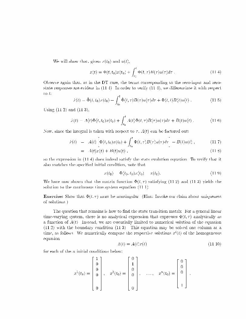
time, as follows. We numerically compute the respective solutions xi(t) of the homogeneous

equation

x_ (t) � A(t)x(t) (11.10)

for each of the n initial conditions below: 3232

1 0

2 3

0

x

1(t0) �

666666664

0

0

777777775

x

2(t0) �

666666664

1

0

777777775

6666664

7777775

0

0� : : : � x

n(t0) � � :0 0 . .. .

.

. .. .

1

0 0

Then h i

�(t� t0) � x1(t) : : : xn(t) : (11.11)

In summary, knowing n solutions of the homogeneous system for n independent initial

conditions, we are able to construct the general solution of this linear time varying system.

The underlying reason this construction works is that solutions of a linear system may be

superposed, and our system is of order n.

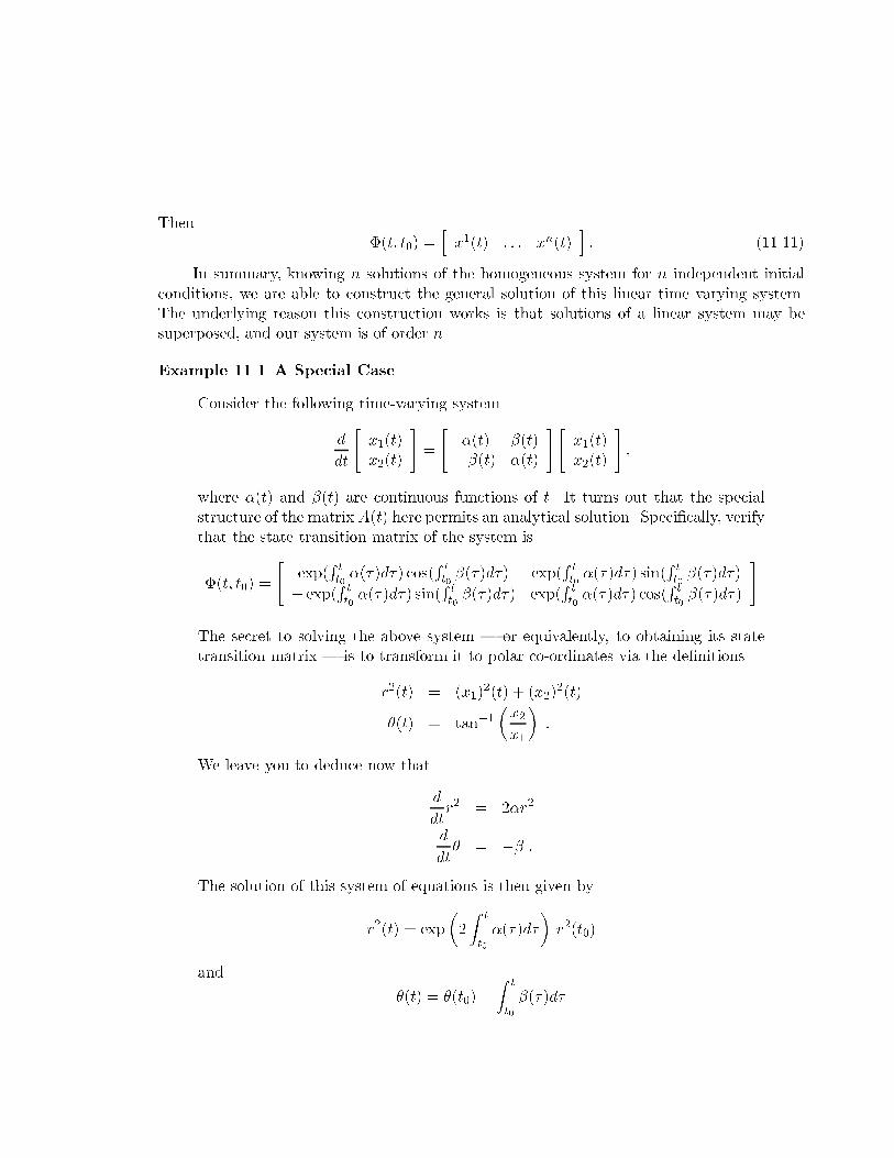
Example 11.1 A Special Case

Consider the following time-varying system " # " # " #

d x1(t) �(t) �(t) x1(t)� �

dt

x2(t) ;�(t) �(t) x2(t)

where �(t) and �(t) are continuous functions of t. It turns out that the special

structure of the matrix A(t) here permits an analytical solution. Speci�cally, verify

that the state transition matrix of the system is " R R R R #

exp(

t �(�)d�) cos(

t �(�)d�) exp(

t �(�)d�) sin(

t �(�)d�)0�(t� t0) �

tR t

Rt0

t

Rtt

0 Rtt

0

; exp( t0

�(�)d�) sin( t0

�(�)d�) exp( �(�)d�) cos( �(�)d�)t0

t0

The secret to solving the above system | or equivalently, to obtaining its state

transition matrix | is to transform it to polar co-ordinates via the de�nitions

r

2(t) � (x1)2(t) + (x2)

2(t)� �

�(t) � tan;1

x2

:

x1

We leave you to deduce now that

d

r

2 � 2�r2

dt

d

� � ;� :

dt

The solution of this system of equations is then given by � Z

�t

r

2(t) � exp 2 �(�)d� r

2(t0)

t0

and Z t

�(t) � �(t0) ; �(�)d�

t0

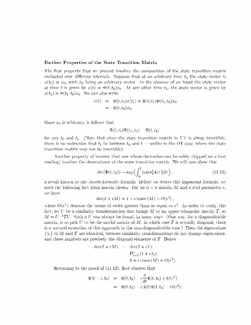
Further Properties of the State Transition Matrix

The �rst property that we present involves the composition of the state transition matrix

evaluated over di�erent intervals. Suppose that at an arbitrary time t0

the state vector is

x(t0) � x0, with x0

being an arbitrary vector. In the absence of an input the state vector

at time t is given by x(t) � �(t� t0)x0. At any other time t1, the state vector is given by

x(t1) � �(t1� t0)x0. We can also write

x(t) � �(t� t1)x(t1) � �(t� t1)�(t1� t0)x0

� �(t� t0)x0:

Since x0

is arbitrary, it follows that

�(t� t1)�(t1� t0) � �(t� t0)

for any t0

and t1. (Note that since the state transition matrix in CT is alway invertible,

there is no restriction that t1

lie between t0

and t | unlike in the DT case, where the state

transition matrix may not be invertible).

Another property of interest (but one whose derivation can be safely skipped on a �rst

reading) involves the determinant of the state transition matrix. We will now show that �Z t

�

det(�(t� t0)) � exp trace[A(�)]d� � (11.12)

t0

a result known as the Jacobi-Liouville formula. Before we derive this important formula, we

need the following fact from matrix theory. For an n � n matrix M and a real parameter �,

we have

det(I + �M) � 1 + � trace (M) + O(�2) �

where O(�2) denotes the terms of order greater than or equal to �2 . In order to verify this

fact, let U be a similarity transformation that brings M to an upper triangular matrix T , so

M � U;1TU . Such a U can always be found, in many ways. (One way, for a diagonalizable

matrix, is to pick U to be the modal matrix of M , in which case T is actually diagonal� there

is a natural extension of this approach in the non-diagonalizable case.) Then the eigenvalues

f�ig of M and T are identical, because similarity transformations do not change eigenvalues,

and these numbers are precisely the diagonal elements of T . Hence

det(I + �M) � det(I + �T )

� �ni�1

(1 + ��i)

� 1 + � trace (M) + O(�2):

Returning to the proof of (11.12), �rst observe that

d

�(t + �� t0) � �(t� t0) + � �(t� t0) + O(�2)dt

� �(t� t0) + �A(t)�(t� t0) + O(�2):

The derivative of the determinant of �(t� t0) is given by

d 1

det[�(t� t0)] � lim (det[�(t + �� t0)] ; det[�(t� t0)])dt

�!0 �

1� �

� lim det[�(t� t0) + �A(t)�(t� t0)] ; det[�(t� t0)]�!0 �

1

� det(�(t� t0)) lim (d et[ I + �A(t)] ; 1)�!0 �

� trace [A(t)] det[�(t� t0)]:

Integrating the above equation yields the desired result, (11.12).

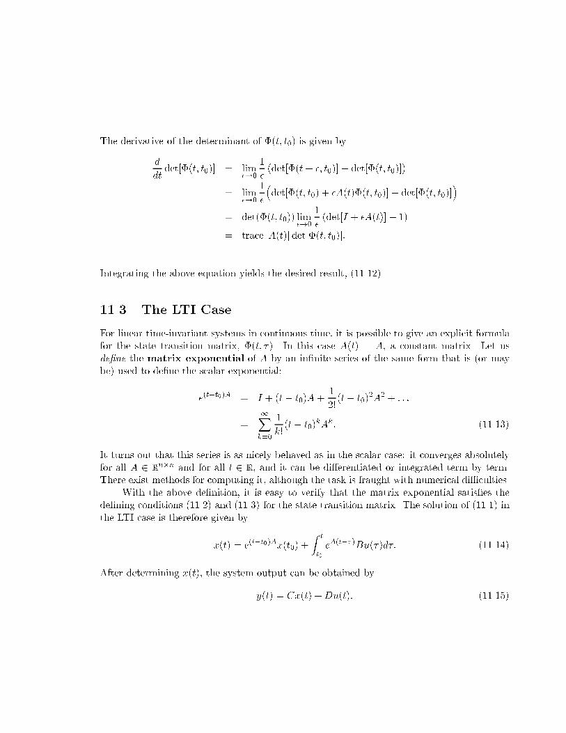
11.3 The LTI Case

For linear time-invariant systems in continuous time, it is possible to give an explicit formula

for the state transition matrix, �(t� �). In this case A(t) � A, a constant matrix. Let us

de�ne the matrix exponential of A by an in�nite series of the same form that is (or may

be) used to de�ne the scalar exponential:

e(t;t0

)A � I + (t ; t0)A +

1(t ; t0)

2A2 + : : :

2!

1X 1

� (t ; t0)kAk: (11.13)

k!

k�0

It turns out that this series is as nicely behaved as in the scalar case: it converges absolutely

for all A 2 Rn�n and for all t 2 R, and it can be di�erentiated or integrated term by term.

There exist methods for computing it, although the task is fraught with numerical di�culties.

With the above de�nition, it is easy to verify that the matrix exponential satis�es the

de�ning conditions (11.2) and (11.3) for the state transition matrix. The solution of (11.1) in

the LTI case is therefore given by Z t

x(t) � e(t;t0

)A x(t0) + e

A(t;�)Bu(�)d�: (11.14)

t0

After determining x(t), the system output can be obtained by

y(t) � Cx(t) + Du(t): (11.15)

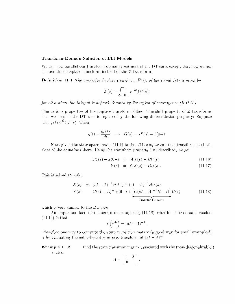
Transform-Domain Solution of LTI Models

We can now parallel our transform-domain treatment of the DT case, except that now we use

the one-sided Laplace transform instead of the Z-transform :

De�nition 11.1 The one-sided Laplace transform, F (s), of the signal f(t) is given by Z 1

F (s) � e;stf(t) dt

t�0;

for all s where the integral is de�ned, denoted by the region of convergence (R.O.C.).

The various properties of the Laplace transform follow. The shift property of Z transforms

that we used in the DT case is replaced by the following di�erentiation property: Suppose

Lthat f(t) �! F (s). Then

df(t)

g(t) � �) G(s) � sF (s) ; f(0;)dt

Now, given the state-space model (11.1) in the LTI case, we can take transforms on both

sides of the equations there. Using the transform property just described, we get

sX(s) ; x(0;) � AX(s) + BU(s) (11.16)

Y (s) � CX(s) + DU(s): (11.17)

This is solved to yield

X(s) � (sI ; A);1 x(0;) + (sI ; A);1BU(s)h i

Y (s) � C(sI ; A);1 x(0;) + C(sI ; A);1B + D U(s) (11.18) | {z }Transfer Function

which is very similar to the DT case.

An important fact that emerges on comparing (11.18) with its time-domain version

(11.14) is that � �

L e

At � (sI ; A);1:

Therefore one way to compute the state transition matrix (a good way for small examples!)

is by evaluating the entry-by-entry inverse transform of (sI ; A);1 .

Example 11.2 Find the state transition matrix associated with the (non-diagonalizable!)

matrix " #

1 2

A � :

0 1

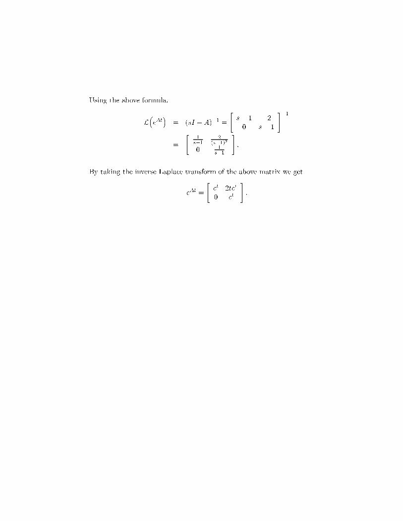
Using the above formula,

L

�

e

At

�

� (sI ; A);1 �

"

s ;

01

s

;;

21

#;1

" #

1 2

�

s;1 (s;1)2

:

0

1

s;1

By taking the inverse Laplace transform of the above matrix we get " #

At �

et 2tet

e :

0 et

Exercises

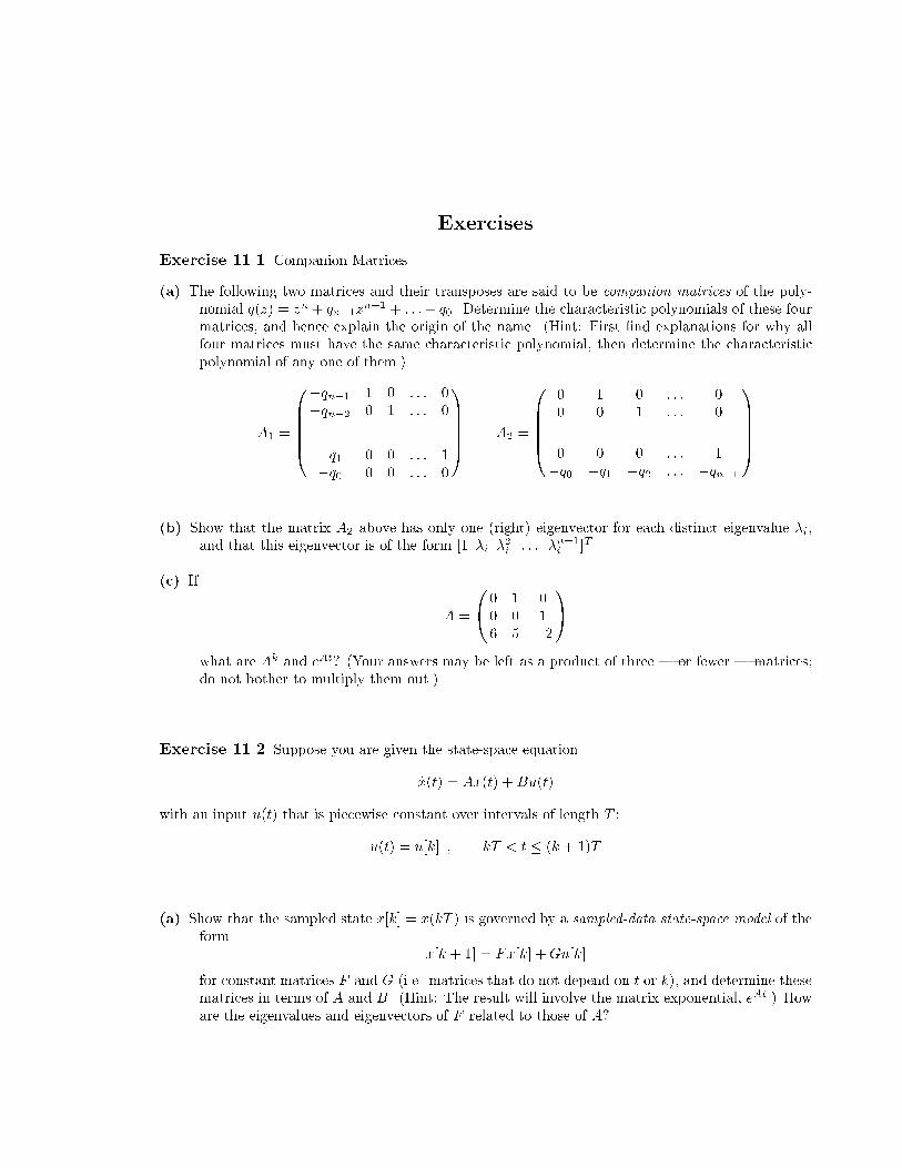
Exercise 11.1 Companion Matrices

(a) The following two matrices and their transposes are said to be companion matrices of the poly-nomial q(z) � zn + qn;1z

n;1 + : : : + q0. Determine the characteristic polynomials of these four

matrices, and hence explain the origin of the name. (Hint: First �nd explanations for why all

four matrices must have the same characteristic polynomial, then determine the characteristic

polynomial of any one of them.) 0 ;qn;1

1 0 : : : 0 101

0 1 0 : : : 0BBBB@

;qn;2

0 1 : : : 0

. . . .

.. . . . .. . .

. .

CCCCA

A2

�

BBBB@

0 0 1 : : : 0

. . . .

. . . . . . . . .

. .

0 0 0 : : : 1

CCCCA

A1

�

0 0 : : : 1

;q1

;q0

0 0 : : : 0

;q0

;q1

;q2

: : : ;qn;1

(b) Show that the matrix A2

above has only one (right) eigenvector for each distinct eigenvalue �i,

and that this eigenvector is of the form [1 �i

�2

i

: : : �ni

;1]T .

(c) If 10

0 1 0

A �

@ 0 0 1

A

6 5 ;2

what are Ak and eAt� (Your answers may be left as a product of three | or fewer | matrices�

do not bother to multiply them out.)

Exercise 11.2 Suppose you are given the state-space equation

x_ (t) � Ax(t) + Bu(t)

with an input u(t) that is piecewise constant over intervals of length T :

u(t) � u[k] � kT � t � (k + 1)T

(a) Show that the sampled state x[k] � x(kT ) is governed by a sampled-data state-space model of the

form

x[k + 1] � Fx[k] + Gu[k]

for constant matrices F and G (i.e. matrices that do not depend on t or k), and determine these

matrices in terms of A and B. (Hint: The result will involve the matrix exponential, eAt.) How

are the eigenvalues and eigenvectors of F related to those of A�

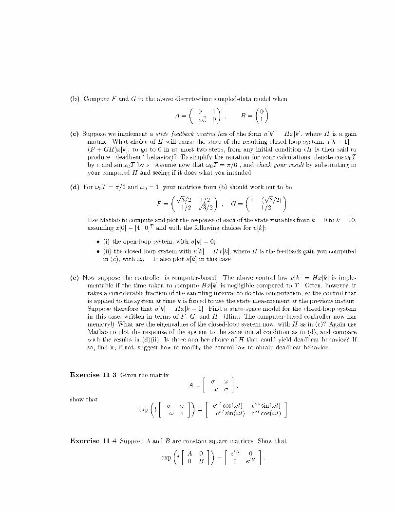
(b) Compute F and G in the above discrete-time sampled-data model when � � � �

0 1 0

A � � B � ;!2 0 10

(c) Suppose we implement a state feedback control law of the form u[k] � Hx[k], where H is a gain

matrix. What choice of H will cause the state of the resulting closed-loop system, x[k + 1] �

(F + GH)x[k], to go to 0 in at most two steps, from any initial condition (H is then said to

produce \deadbeat" behavior)� To simplify the notation for your calculations, denote cos !0T

by c and sin !0T by s. Assume now that !0T � ��6 , and check your result by substituting in

your computed H and seeing if it does what you intended.

(d) For !0T � ��6 and !0

� 1, your matrices from (b) should work out to be

F �

� p3�2 p1�2

� �

1 ; (p3�2)

�

� G � ;1�2 3�2 1�2

Use Matlab to compute and plot the response of each of the state variables from k � 0 to k � 10,

assuming x[0] � [4 � 0]T and with the following choices for u[k]:

� (i) the open-loop system, with u[k] � 0�

� (ii) the closed-loop system with u[k] � Hx[k], where H is the feedback gain you computed

in (c), with !0

� 1� also plot u[k] in this case.

(e) Now suppose the controller is computer-based. The above control law u[k] � Hx[k] is imple-mentable if the time taken to compute Hx[k] is negligible compared to T . Often, however, it

takes a considerable fraction of the sampling interval to do this computation, so the control that

is applied to the system at time k is forced to use the state measurement at the previous instant.

Suppose therefore that u[k] � Hx[k ; 1]. Find a state-space model for the closed-loop system

in this case, written in terms of F , G, and H . (Hint: The computer-based controller now has

memory!) What are the eigenvalues of the closed-loop system now, with H as in (c)� Again use

Matlab to plot the response of the system to the same initial condition as in (d), and compare

with the results in (d)(ii). Is there another choice of H that could yield deadbeat behavior� If

so, �nd it� if not, suggest how to modify the control law to obtain deadbeat behavior.

Exercise 11.3 Given the matrix � �

A �

�

;!

!

�

�

show that

exp

�

t

�

�

;!

!

�

��

�

�

e�t

;e�

cos(!t)

t sin(!t)

e�t

e�t

sin(!

cos(!

t)

t)

�

Exercise 11.4 Suppose A and B are constant square matrices. Show that � � �� � �

A 0 etA 0

exp t � :

0 B 0 etB

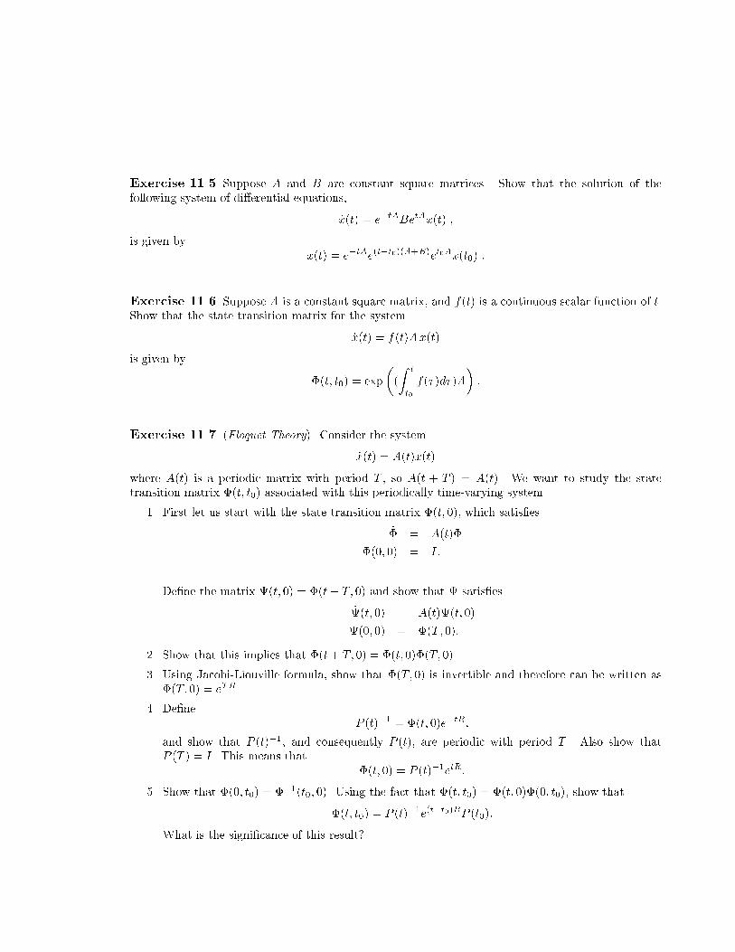
Exercise 11.5 Suppose A and B are constant square matrices. Show that the solution of the

following system of di�erential equations,

x_ (t) � e;tABe

tA x(t) �

is given by

x(t) � e;tA e(t;t0

)(A+B)e

t0

A x(t0) :

Exercise 11.6 Suppose A is a constant square matrix, and f(t) is a continuous scalar function of t.

Show that the state transition matrix for the system

x_ (t) � f(t)Ax(t)

is given by � Z t

�

�(t� t0) � exp ( f(�)d�)A :

t0

Exercise 11.7 (Floquet Theory). Consider the system

x_ (t) � A(t)x(t)

where A(t) is a periodic matrix with period T , so A(t + T ) � A(t). We want to study the state

transition matrix �(t� t0) associated with this periodically time-varying system.

1. First let us start with the state transition matrix �(t� 0), which satis�es

_� � A(t)�

�(0� 0) � I:

De�ne the matrix �(t� 0) � �(t + T� 0) and show that � satis�es

_�(t� 0) � A(t)�(t� 0)

�(0� 0) � �(T� 0):

2. Show that this implies that �(t + T� 0) � �(t� 0)�(T� 0).

3. Using Jacobi-Liouville formula, show that �(T� 0) is invertible and therefore can be written as

�(T� 0) � eTR .

4. De�ne

P (t);1 � �(t� 0)e;tR�

and show that P (t);1 , and consequently P (t), are periodic with period T . Also show that

P (T ) � I . This means that

�(t� 0) � P (t);1 e

tR:

5. Show that �(0� t0) � �;1(t0� 0). Using the fact that �(t� t0) � �(t� 0)�(0� t0), show that

�(t� t0) � P (t);1 e(t;t0

)RP (t0):

What is the signi�cance of this result�

MIT OpenCourseWarehttp://ocw.mit.edu

6.241J / 16.338J Dynamic Systems and Control Spring 2011

For information about citing these materials or our Terms of Use, visit: http://ocw.mit.edu/terms.