5/24/2015© 2009 raymond p. jefferis iii lect 05 - 1 geographic image processing data transformation...

04/18/23 © 2009 Raymond P. Jefferis III Lect 05 - 1

Geographic Image Processing

Data Transformationand Filtering• Noise in data• Arrays• Digital filtering• Filter coefficients• Convolution• Topographic map

Gaussian Convolution Filter Coefficients

1 4 8 10 8 4 14 12 23 28 23 12 48 23 43 54 43 23 8

10 28 54 67 54 28 10 /9398 23 43 54 43 23 84 12 23 28 23 12 41 4 8 10 8 4 1


Types of Image Noise

• Distributed random (altitude uncertainty)– Gaussian (many physical measurements)– Uniform (useful for models and tests)

• Impulse noise (natural data disturbances)

• Salt-and-Pepper (random 0s and 1s)


Noisy Data

In the slide to follow, – the first image shows DTED raw data, as

distributed– the second image shows the same data

corrupted by uniform random noise of ± 5 meters

Note: Raw DTED data has noise of less than ±1 meter


Uniform Random Data Noise

Normal DTED Data Noisy DTED Data


Effects of Noise

• Greater uncertainty in data

• Cascading uncertainty in computations performed on data:– Topographical maps– Attribute contours (contour maps)– Watershed gradients


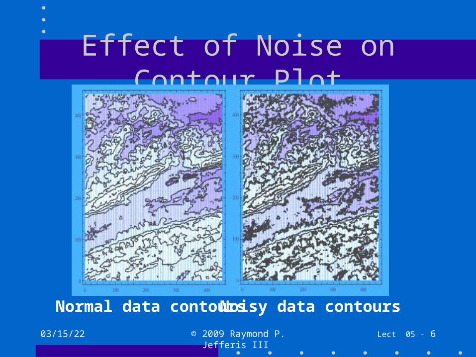
Effect of Noise on Contour Plot

Normal data contours Noisy data contours


Gaussian Noise (Mean=0, StdDev=5)

Noisy DTED Data Noisy data contours


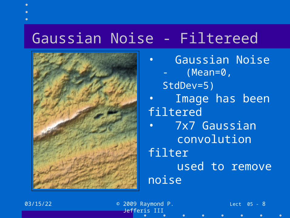
Gaussian Noise - Filtereed• Gaussian Noise

- (Mean=0, StdDev=5) • Image has been filtered• 7x7 Gaussian

convolution filterused to remove noise


Notes on Noise

• Contour maps frequently give contours 25 - 50 meters apart. If data points are not smoothed to this distance, contours will appear jagged

• Data points are on 10-meter centers, depending on type of noise, a recommended convolution array might be at least 11x11.


Raw and Averaged Contours

Raw Data - Malvern 3x3 Convolution


Effect of 7x7 vs 15x15 Convolutes

15x15 Gaussian filter7x7 Gaussian filter


Reasons for Digital Filtering

• Reduction of random noise• Smoothing of topological contours• Smoothing topological cross-sections• Smoothing of attribute contours (rainfall, etc.)• Smoothing of data for gradient calculations• To extract image features or attributes• To enhance image features or attributes


What is digital filtering?• Processing of raw data

• Uses filter algorithms

• Filters typically require coefficients to control the data processing

• Convolution methods frequently used for image processing (can be parallelized)

• Data combined from multiple points/sources


The Meaning of Digital Filtering

• Points in an image field contain noise• Each single point is physically related to its

surrounding points, so that sudden spatial changes are improbable

• Digital filtering exploits this relationship by adding information from surrounding points to the central points by means of a weighted summation process - convolution.


Convolution Filter• Uses an array of filter weights• Operated incrementally over entire data

field, except near edges of data• Each resulting point is sum of weighted

data surrounding it, divided by sum of weights (normalized weights, shifted for convolution)( ∑ Data*Weights / ∑ Weights )

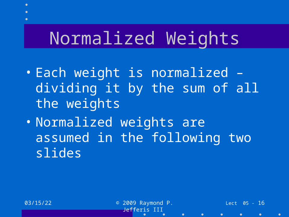
Normalized Weights

• Each weight is normalized – dividing it by the sum of all the weights

• Normalized weights are assumed in the following two slides



Discrete Convolution

h[i, j] =d[i, j] * w[i, j]

h[i, j] = d[k, l]g[i −k, j −l]l=1

m

∑k=1

n

∑


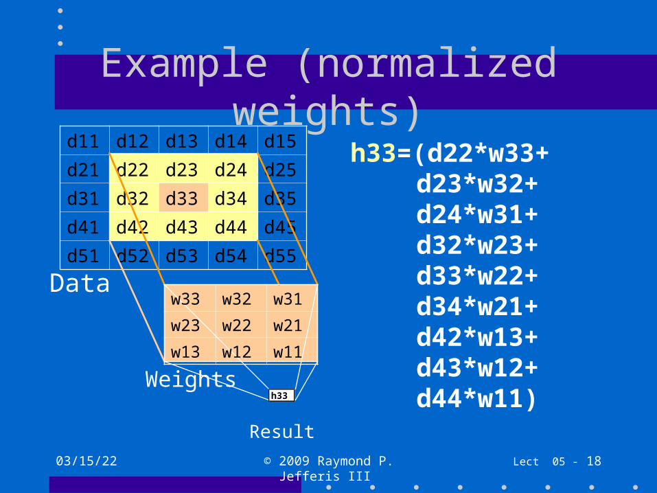
Example (normalized weights)d11 d12 d13 d14 d15

d21 d22 d23 d24 d25

d31 d32 d33 d34 d35

d41 d42 d43 d44 d45

d51 d52 d53 d54 d55

h33=(d22*w33+d23*w32+d24*w31+d32*w23+d33*w22+d34*w21+d42*w13+d43*w12+d44*w11)

Data

Weights

Result

w33 w32 w31

w23 w22 w21

w13 w12 w11

h33


Example: Gaussian Image Filter

• Determine filter coefficients from spatial Gaussian function.

• Form convolution matrix

• Normalize coefficients

• Convolve matrix with spatial data

• Obtain filtered result for each image pixel


Result

• Convolution operation performed

• Gaussian filter kernel (square matrix with odd number of rows and columns)

• Gauss filter smooths or blurs an image


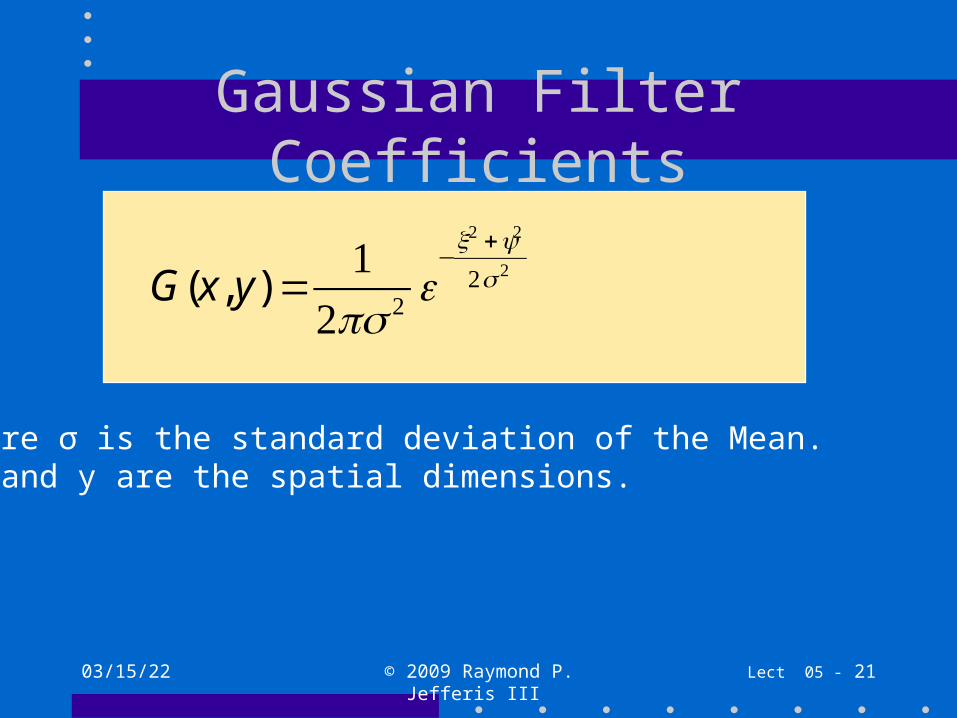
Gaussian Filter Coefficients

G(x, y) =1

2πσ 2 e−

x2 +y2

2σ 2

Here σ is the standard deviation of the Mean. x and y are the spatial dimensions.


Calculation of Gaussian Weightss = 1.52; im = 3; nrm = 0;For[j = -im, j < im + 1, j++,]Print[nrm]

For[i = -im, i < im + 1, i++, g = Exp[-((i^2 + j^2)/(2.0* s^2))]; gr = Round[g*67]; Print[gr]; nrm = nrm + gr; ]Notes:See Models file for program.Degree of smoothing determines by value of “s”


Choice of Parameters

• Pick (odd) number of samples

• Pick σ to broaden filter to desired number of samples

• Pick multiplier (67 in example) to give unity coefficients at edges.

• Repeat until filter exhibits desired smoothing


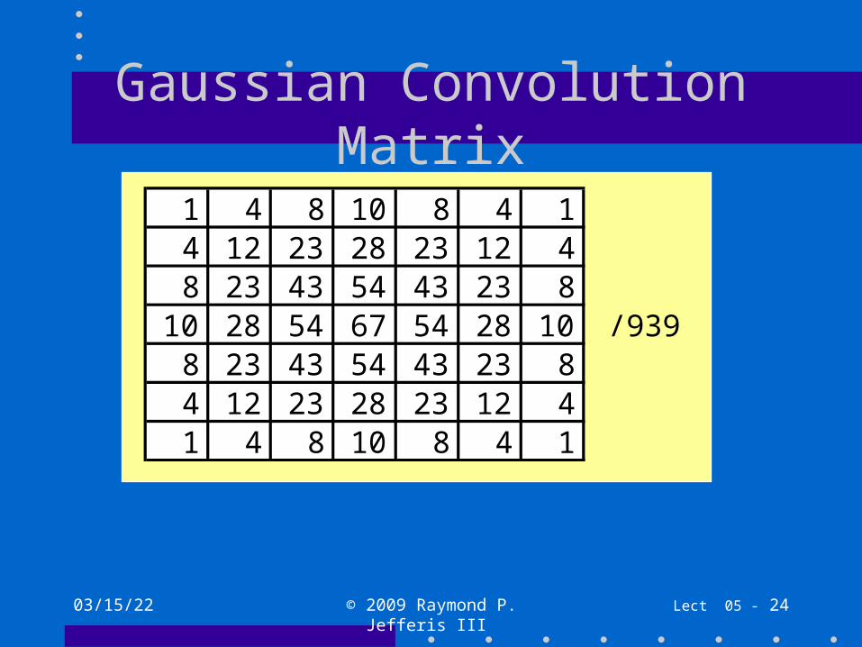
Gaussian Convolution Matrix

1 4 8 10 8 4 14 12 23 28 23 12 48 23 43 54 43 23 8

10 28 54 67 54 28 10 /9398 23 43 54 43 23 84 12 23 28 23 12 41 4 8 10 8 4 1


Notes

• Central points have higher weight

• Diagonal points have weights reduced (distance to central point is longer)

• Whole number weights used, though NOT necessary. Normalized weights are Real numbers.


Comments

• Coefficients are typically whole numbers

• Sum of coefficients normalizes them, resulting in array of Real numbers

• Example filter gives most weight to central data (little blurring)


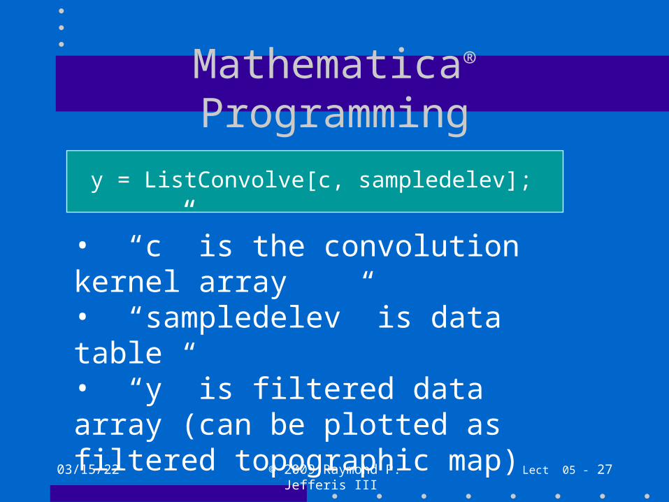
Mathematica® Programming

y = ListConvolve[c, sampledelev];

• “c” is the convolution kernel array• “sampledelev” is data table• “y” is filtered data array (can be plotted as filtered topographic map)

Note

• If data matrix is m x m, and

• Convolution kernel is (2n+1) x (2n+1), then

• The filtered result will be (m-n) x (m-n)

• Example:m = 4802n +1 = 17Result is (480 - 8) x (480 - 8)



Filtering Malvern Data

Normal DTED Data Filtered DTED Data


Comments on Filtering

• Gaussian filtering will remove some degree of random noise

• Resulting image will have some blurring, when compared with (noise-free) unfiltered data

• Convolution filtering with n x n kernel will reduce image size by 2*(n-1) pixels in both horizontal and vertical directions.


Filtering A Noisy Image

±5m Noisy DTED Data Filtered Noisy Data


High Noise Levels

• Gaussian filtering can remove a lot of noise!

• Resulting image may look quite sharp or may be blurred


Filtering Very Noisy Image

±10m Noisy DTED Data Filtered Very Noisy Data


Topographic Map

• Shows contours of equal altitude

• Fixed contour spacing

• Similar to horizontal “slices” through the topography

• Requires smooth (filtered) data


Filtered Topographic Map

• Malvern quadrangle

• Filtered data used• Gaussian 7 x 7

convolution filter (s = 1.52)

• Contour lines at 20-meter intervals


Comment on Contour Map

• Edges are a little jaggy

• More filtering (smoothing) would be preferable, to get smooth contours

• 11x11 or 15x15 convolution kernels would be preferred

Questions?


5/24/2015© 2009 raymond p. jefferis iii lect 05 - 1 geographic image processing data transformation...

Documents

noise slide

filtering noise

parallelized data

dted raw data

raw dted data

processing of raw data

effect of noise

jagged data points