lect 02© 2012 raymond p. jefferis iii1 satellite communications orbital calculations orbit...

Lect 02 © 2012 Raymond P. Jefferis III 1

Satellite CommunicationsOrbital Calculations• Orbit definition & properties• Kepler’s Laws

• First Law• Second Law• Third Law

• Coordinate Systems• Geocentric

equatorial• Astronomical

• Satellite location• Geostationary orbits• Look angle calculations• Doppler shift

GALAXY-11 Satellite, Hughes Space and Communications


Orbit Definition and Properties

• An orbit is a stable path around the earth traversed periodically by a satellite above the atmosphere of the earth.

• Orbits are elliptical

• Orbits have an Eccentricity parameter

• Certain orbital properties are described by Keppler’s laws

Definition of Ellipse

• An ellipse is a regular oval shape, traced by a point moving in a plane so that the sum of its distances from two other points (the foci) is constant.

Lect 02 © 2012 Raymond P. Jefferis III Lect 00 - 3

Axes of Ellipse


b a

b

a

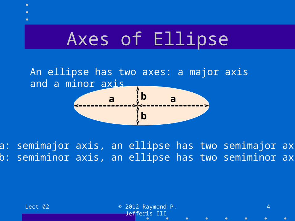
a: semimajor axis, an ellipse has two semimajor axesb: semiminor axis, an ellipse has two semiminor axes

An ellipse has two axes: a major axis and a minor axis

Ellipse Properties

• The sum of the distances from any point P on an ellipse to its two foci is constant and equal to the major diameter

• The eccentricity of an ellipse is the ratio of the distance between the two foci and the length of the major axis



Kepler’s First Law• A satellite, as a secondary body, follows an

elliptical path around a primary body (earth).• The center of mass of the two bodies, the

barycenter, will be at one of the foci.• For semimajor axis a and semiminor axis b, the

orbital eccentricity e is be expressed by,

e =a−ba+b

=a2 −b2

a


Kepler’s Second Law

• A ray from the barycenter to an orbiting satellite will sweep out equal areas in the orbital plane in equal time intervals.


Kepler’s Third Law

• The square of the orbital time is proportional to the cube of the mean distance, a, between the two bodies (semimajor axis). For a satellite motion of n radians/sec (orbital period P = 2π/n) and the gravitational parameter of the earth, G*M = μ= 3.986004418E5 km3/s2, then the mean distance, a, is calculated as,

a3 =μn2 =

μP2

4π 2

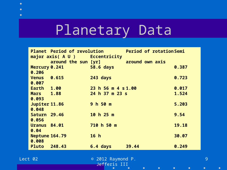
Planetary Data


Planet Period of revolution Period of rotation Semi major axis( A U ) Eccentricityaround the sun [yr] around own axis

Mercury 0.241 58.6 days 0.387 0.206Venus 0.615 243 days 0.723 0.007Earth 1.00 23 h 56 m 4 s 1.00 0.017Mars 1.88 24 h 37 m 23 s 1.524 0.093Jupiter 11.86 9 h 50 m 5.203 0.048Saturn 29.46 10 h 25 m 9.54 0.056Uranus 84.01 710 h 50 m 19.18 0.04Neptune 164.79 16 h 30.07 0.008Pluto 248.43 6.4 days 39.44 0.249

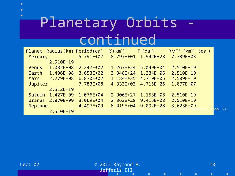
Planetary Orbits - continued


Planet Radius(km) Period(da) R3(km3) T2(da2) R3/T2 (km3) (da2) Mercury 5.791E+07 8.797E+01 1.942E+23 7.739E+03 2.510E+19 Venus 1.082E+08 2.247E+02 1.267E+24 5.049E+04 2.510E+19 Earth 1.496E+08 3.653E+02 3.348E+24 1.334E+05 2.510E+19 Mars 2.279E+08 6.870E+02 1.184E+25 4.719E+05 2.509E+19 Jupiter 7.783E+08 4.333E+03 4.715E+26 1.877E+07 2.512E+19 Saturn 1.427E+09 1.076E+04 2.906E+27 1.158E+08 2.510E+19 Uranus 2.870E+09 3.069E+04 2.363E+28 9.416E+08 2.510E+19 Neptune 4.497E+09 6.019E+04 9.092E+28 3.623E+09 2.510E+19

Computations by Neal McLain, Society of Broadcast Engineers, Chap. 24.

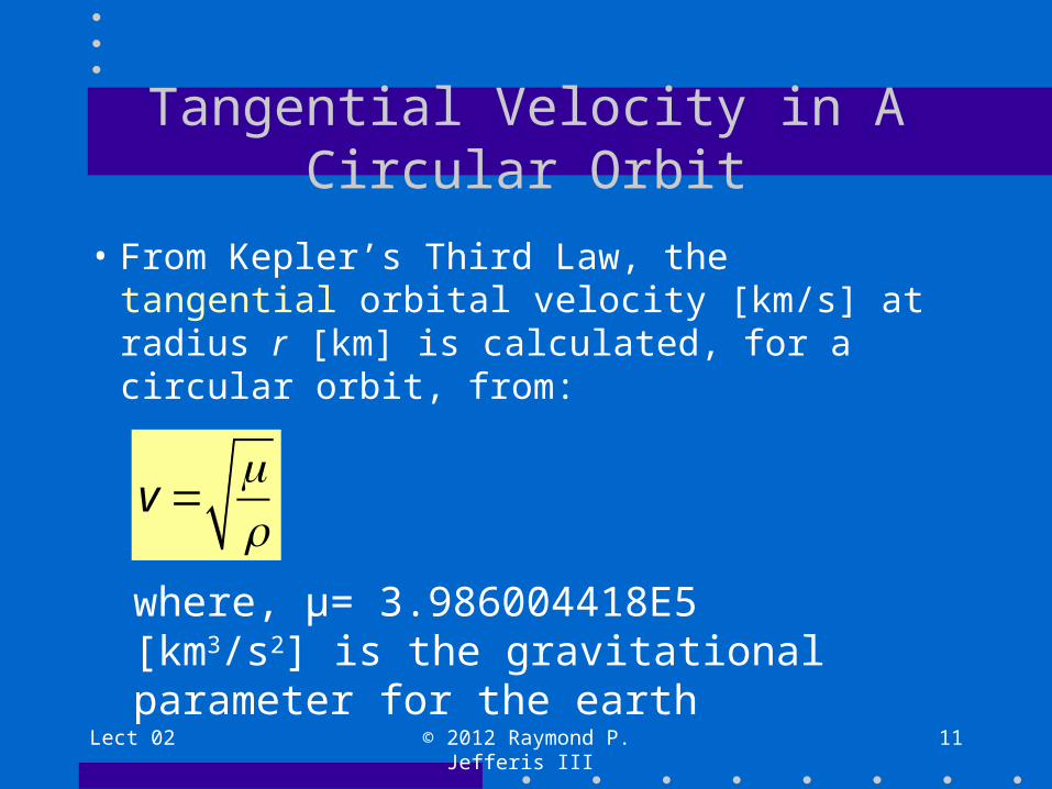
Tangential Velocity in A Circular Orbit

• From Kepler’s Third Law, the tangential orbital velocity [km/s] at radius r [km] is calculated, for a circular orbit, from:


v =μr

where, μ= 3.986004418E5 [km3/s2] is the gravitational parameter for the earth

Tangential Velocity Calculation

• r = 42, 164.17 [km] - geostationary orbit

• μ= 3.986004418E5 [km3/s2]

• v = 3.0746600858 [km/s]



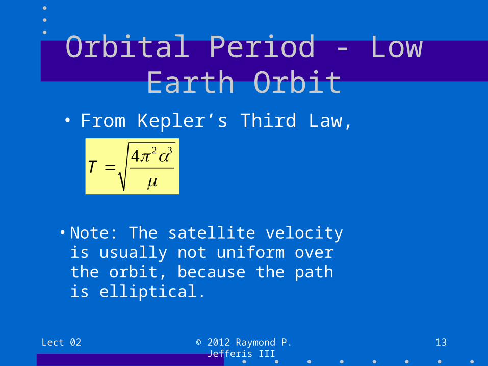
Orbital Period - Low Earth Orbit

• From Kepler’s Third Law,

T =4π 2a3

μ

• Note: The satellite velocity is usually not uniform over the orbit, because the path is elliptical.


Example - Space Station

For the International Space Station with altitudeh = 350 km,

• a = re + h = 6378.14 + 350 = 6728.14 km. μ= 3.986004418E5 km3/s2

• T = 5492.29 sec/orbit (91.538 min/orbit)• 1/T =15.69 orbits/sidereal day (15.73 orbits in 24

hours)


Elliptical Orbit Calculation• The satellite NOAA-B (1980-43A) was launched in May

1980 into an orbit with perigee height of 260 km and apogee height 1440 km.

• We wish to find the orbital period and the orbital eccentricity.

• Data:2a = 2re+hp + ha = 2(6378.14)+260+1440 = 14456.28 km

• Calculations:a = 7228.14 kmT = 6115.77 sec/orbite = 1 - (re+hp)/a = 0.0816254

Sample Orbital Calculation

mu = 3.986004418 10^5;

ha = 1440.0;hp = 260.0;re = 6378.14;twoa = 2*re + hp + ha;a = twoa/2;t = Sqrt[(4*pi^2*a^3)/mu];tinv = 24*60*60/t;ecc = 1.0 - (re + hp)/a;


Two-Line Data Element Set (TLE)

• The two-line element set (TLE) is a data format that lists information pertaining to the orbital parameters of Earth-orbiting satellites.

• TLE format is used by NORAD and NASA• TLE data can be used, with appropriate software,

to compute satellite position at a given time• Models used: SGP4 or SGP8

Lect 02 © 2012 Raymond P. Jefferis III \Lect 00 - 17

NASA Satellite Data - TLE

• Line 1– Col 3 - 7 Satellite number

– Col 19-20 Epoch year (last two digits)

– Col 21-32 Epoch Day and fraction

– Col 34-43 Mean motion derivative [rev/day 2]


NASA Satellite Data - TLE

• Line 2– Col 9 –16 Inclination [degrees]

– Col 18-25 Right ascension [degrees]

– Col 27-33 Eccentricity – leading decimal assumed

– Col 35-42 Argument of perigee [degrees]

– Col 44-51 Mean anomaly [degrees]

– Col 53-63 Mean motion [rev/day]

– Col 64-68 Revolution number at epoch [rev]


Spacetrack (SGP4) Reference

http://www.amsat.org/amsat/ftp/docs/spacetrk.pdf

SPACETRACK REPORT NO. 3

Models for Propagation of NORAD Element Sets

Felix R. Hoots and Ronald L. Roehrich

December 1980

Package Compiled by

TS Kelso

31 December 1988

Lect 02 © 2012 Raymond P. Jefferis III Lect 00 - 20


Geosynchronous Orbits

• A geosynchronous orbit is an orbit (usually equatorial) having a period of one sidereal day, 23h 56m 04.0905s (23.9344695833 hours, or 86164.090530833 seconds).

• A siderial day is the rotation of the earth in relation to the (relatively fixed) position of the stars. Shorter than solar day.


Polar Orbits• A polar orbit is an orbit that passes over (or nearly

passes over) both North and South poles.– Can be sun-synchronous (heliosynchronous)– Has a low altitude (800 - 1000 km), that is

slightly retrograde, and leads to high resolution images with approximately constant illumination angles

– Used for weather, environmental, and spy satellites


Radius of Geostationary Orbit• A geosynchronous orbit has a period of one

sidereal day, T = 86164.090530833 seconds

• The radius is given by,

a =

μT2

4π 23

• So a = 42, 164.17 km.


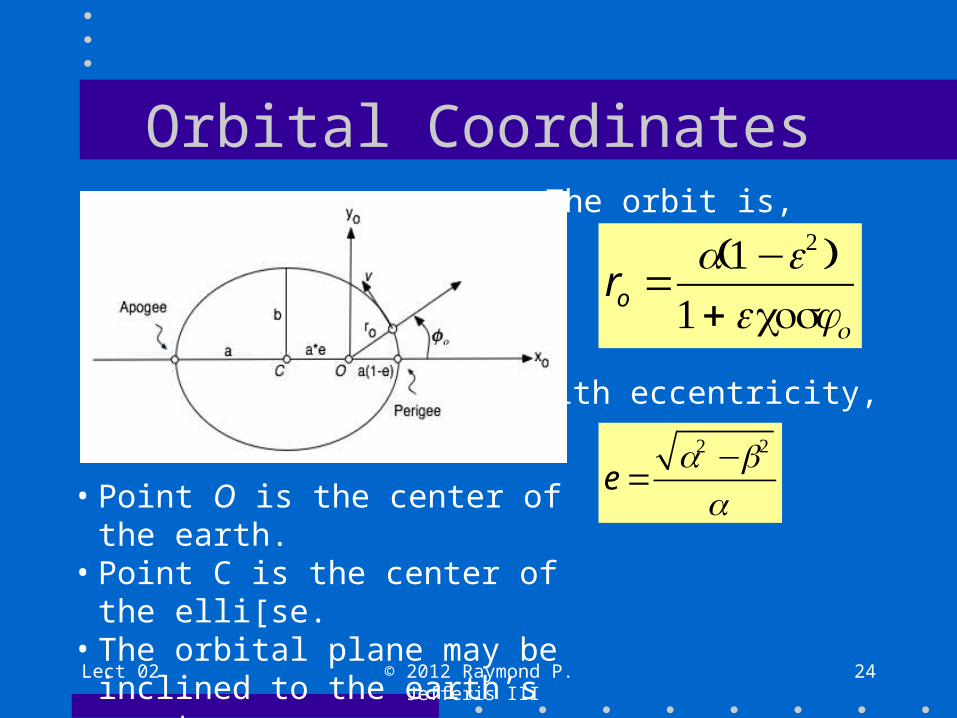
Orbital Coordinates

• Point O is the center of the earth.• Point C is the center of the elli[se.• The orbital plane may be inclined to

the earth’s equator.

ro =a(1−e2 )1+ ecosφo

The orbit is,

With eccentricity,

e =a2 −b2

a


Other Calculations• Apogee height (radius), ra = a(1+e) • Perigee height (radius), rp = a(1-e)• The flight path angle, θis,

θ =arctanesinφo

1+ ecosφo

⎛

⎝⎜⎞

⎠⎟


Orbital Velocity

• The gravitational product G*M for the earth is G*M = μ = 3.986004418E14 [m3/s2]

• The gravitational acceleration g is,g = G*M/r2 = 6.67259E-11 [N-m2/kg2]

• The tangential velocity is, then,

v =GMa(1−e2 )ro cosφo

Definitions


Coordinate Reference

• x-axis is directed at “First Point of Ares”– Direction to Ares at vernal equinox defines the

zero point of Right Ascension to the satellite

• z-axis is directed along the spin axis of the earth– Approximately toward the North Star

• y-axis is orthogonal to x-axis and z-axis


Rectangular Geocentric Coordinates


Spherical Geocentric Coordinates


α is right ascension to satellite

δ is declinationto satellite

Rectangular – Spherical Relation



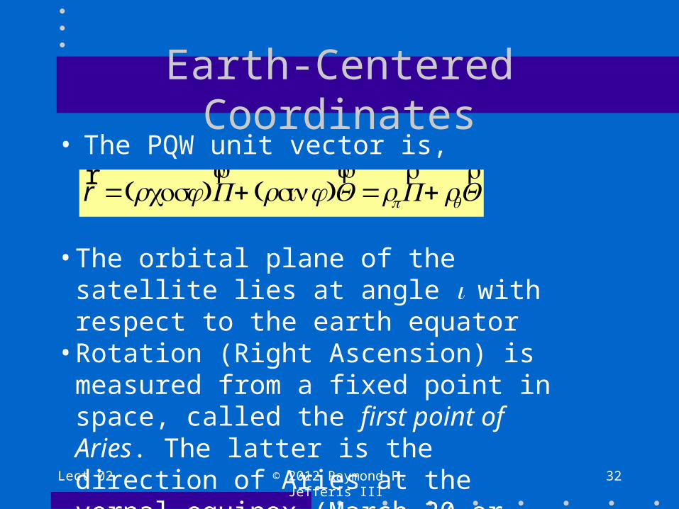
Earth-Centered Coordinates• The PQW unit vector is,

rr =(rcosφ)P

ur+ (rsinφ)Q

ur=rp

rP + rq

rQ

• The orbital plane of the satellite lies at angle with respect to the earth equator

• Rotation (Right Ascension) is measured from a fixed point in space, called the first point of Aries. The latter is the direction of Aries at the vernal equinox (March 20 or 21)

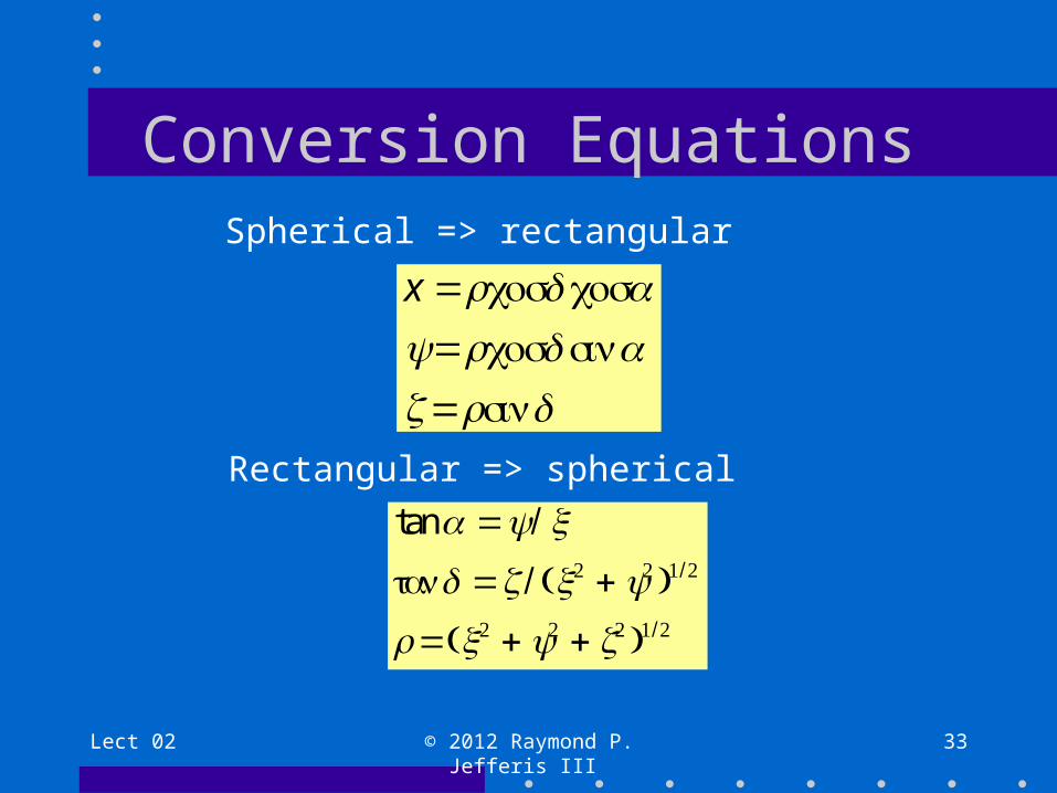
Conversion Equations


x =rcosδ cosαy=rcosδ sinαz=rsinδ

Spherical => rectangular

Rectangular => spherical

tanα =y/ x

tanδ =z / (x2 + y2 )1/2

r =(x2 + y2 + z2 )1/2


Transformation

rI

rJ

rK

⎡

⎣

⎢⎢⎢

⎤

⎦

⎥⎥⎥=R

ur rPrQ

⎡

⎣⎢

⎤

⎦⎥

where,

Rur=

(cosΩcosω −sinΩsinω cosi) (−cosΩsinω −sinΩcosω cosi)(sinΩcosω + cosΩsinω cosi) (−sinΩsinω + cosΩcosω cosi)

(sinω sini) (cosω sini)

⎡

⎣

⎢⎢⎢

⎤

⎦

⎥⎥⎥

rPrQ

⎡

⎣⎢

⎤

⎦⎥

The transformation to earth coordinates is,


Orbital Position Description

In-Class Example


Calculate orbital position indicated in Roddy Example 2.16


Example (Roddy, Example 2.16)

• DataΩ = 300˚, ω = 60˚, i = 65˚, rP = -6500 km, rQ = 4000 km

r = rP

2 + rQ2 =7632.2km


Calculation for Roddy ExampleW = 300.0 Degree;r = {{-6500.0}, {4000.0}}R = {{(Cos[W] Cos[w] - Sin[W] Sin[w] Cos[i]),

(-Cos[W] Sin[w] - Sin[W] Cos[w] Cos[i])}, {(Sin[W] Cos[w] + Cos[W] Sin[w] Cos[i]), (-Sin[W] Sin[w] + Cos[W] Cos[w] Cos[i])}, {(Sin[w] Sin[i]), (Cos[w] Sin[i])}}

v = R.r = {{-4685.32}, {5047.71}, {-3289.14}}vmag = Sqrt[v[[1]]^2 + v[[2]]^2 + v[[3]]^2]

= {7632.17}

w = 60.0 Degree;i = 65.0 Degree;


Satellite Look Angles

• The subsatellite point (SSP) is the intersection of the orbital radius line with the earth surface.

• An earth station will lie at an angle Υto the zenith from earth center to satellite and at azimuth angle Az to True North.

• The satellite will be seen at elevation angle El to the local horizontal at the earth station

• Visibility requires positive El, otherwise it is below the horizon


Look Angle Geometry

Look angle geometry, after Pratt et al


Look Angle Calculations

cosγ =cosLatES cosLatSat cos(LonSat −LonES) + sinLatES sinLatSat

El =ψ −90o

d =rs 1+rers

⎛

⎝⎜⎞

⎠⎟

2

−2rers

⎛

⎝⎜⎞

⎠⎟cosγ

⎡

⎣⎢⎢

⎤

⎦⎥⎥

1/2

The communications path length, d, along which path losses will be calculated is calculated from:

The elevation above Earth Station vertical is,

By the Law of Cosines,


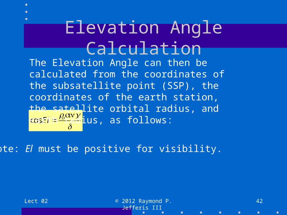
Elevation Angle Calculation

cos El =rssinγ

d

The Elevation Angle can then be calculated from the coordinates of the subsatellite point (SSP), the coordinates of the earth station, the satellite orbital radius, and earth radius, as follows:

Note: El must be positive for visibility.


Geostationary Orbit Case

• In this case the subsatellite point is on the Equator at longitude Lons, while Lats = 0.

• rs = 42,164.17 km (geosynchronous)

• re = 6378.137 km

• rs/re = 6.6107345

• These reduce the calculations to those on the following slide:


Geostationary Calculationscosγ =cosLatES cos(LonS −LonES)

d=rs[1.02288235 −0.30253825cosγ]12

El =tan−1[(6.6107345 −cosγ) / sinγ] −γ

α =tan−1 tan LonS −LonES

sinLatES

⎡

⎣⎢

⎤

⎦⎥

Ref: Pratt, et al, §2.2


Visibility Conditions

• The Elevation angle, El, must be positive

• or,

γ ≤cos−1 re

rs

⎛

⎝⎜⎞

⎠⎟


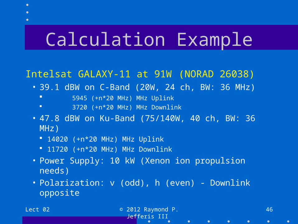
Calculation Example

Intelsat GALAXY-11 at 91W (NORAD 26038)

• 39.1 dBW on C-Band (20W, 24 ch, BW: 36 MHz) 5945 (+n*20 MHz) MHz Uplink 3720 (+n*20 MHz) MHz Downlink

• 47.8 dBW on Ku-Band (75/140W, 40 ch, BW: 36 MHz) 14020 (+n*20 MHz) MHz Uplink 11720 (+n*20 MHz) MHz Downlink

• Power Supply: 10 kW (Xenon ion propulsion needs)

• Polarization: v (odd), h (even) - Downlink opposite


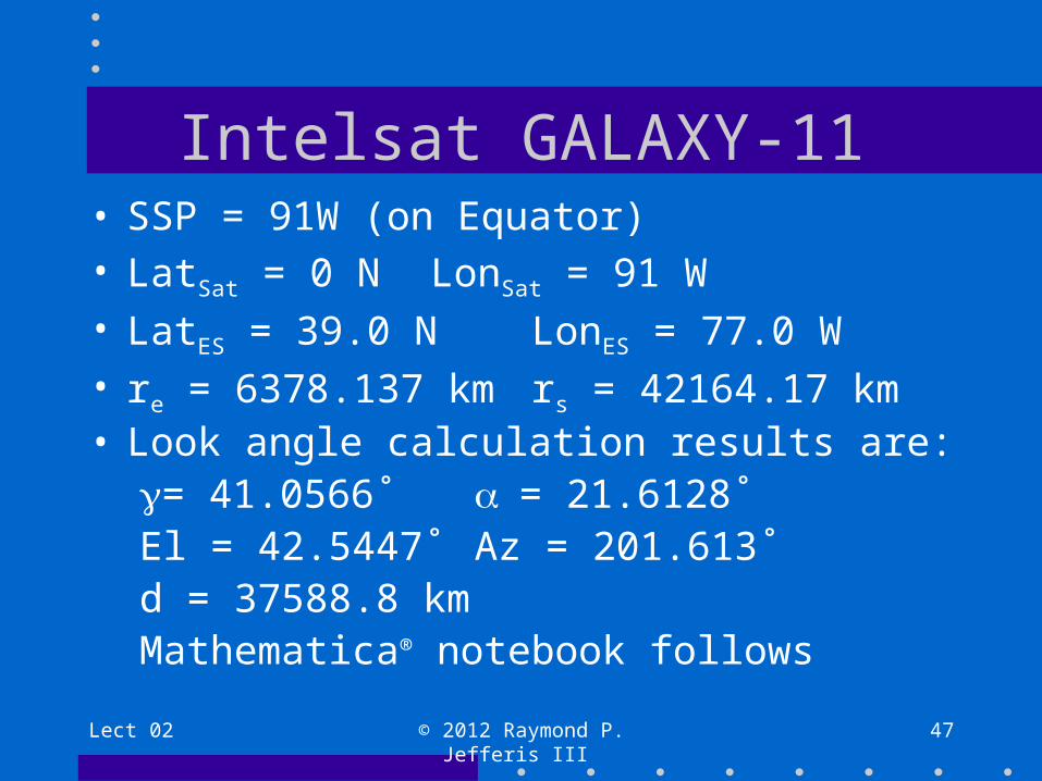
Intelsat GALAXY-11• SSP = 91W (on Equator)• LatSat = 0 N LonSat = 91 W• LatES = 39.0 N LonES = 77.0 W• re = 6378.137 km rs = 42164.17 km• Look angle calculation results are:

γ= 41.0566˚ α= 21.6128˚El = 42.5447˚ Az = 201.613˚d = 37588.8 kmMathematica® notebook follows


Galaxy-11 Look Angle Calculationsre = 6378.137; rs = 42164.17;rr = re/rs;lates = 39.0 Degree; lones = -77.0 Degree;latsat = 0.00 Degree; lonsat = -91.0 Degree; gam = ArcCos[Cos[lates]*Cos[latsat]*Cos[lonsat

-lones] + Sin[lates]*Sin[latsat]];d = rs*Sqrt[1 + rr^2 - 2.0*rr*Cos[gam]];el = ArcCos[rs*Sin[gam]/d];alpha = ArcTan[Tan[Abs[lonsat-lones]]/Sin[lates]];az = 180 + alpha/Degree

Notes on More Accurate Calculations

• Alternative equations are available:– Roddy, D., Satellite Communications, McGraw-Hill,

2006, §3.2.

• Equations are also available that include the earth station altitude, for greater accuracy:– Ippolito, L., Satellite Communications Systems

Engineering, Wiley, 2008, §2.4.


Class Problem – Workshop 02• Earth Station: Washington, DC

– Latitude: Late = 38.895° N (+38.895°)

– Longitude: Lone = 77.0363° W (-77.0363°)

• Satellite: Geosynchronous at 91W– Latitude: Lats = 0° (+0°)

– Longitude: Lons = 91° W (-91°)

• Find range, elevation, and azimuth angle from the earth station to the satellite


Work on the Problem

• Take 45minutes

• Formulate your answers as follows:– Elevation– Azimuth– Range

• Hand in next week as a brief report for Workshop credit.


Workshop 02 Calculations


re = 6378.137; rs = 42164.17;rr = re/rs;lates = 38.895 Degree; lones = -77.0363 Degree;latsat = 0.0 Degree; lonsat = -91.0 Degree;gam = ArcCos[Cos[lates]*Cos[latsat]*Cos[lonsat -

lones] + Sin[lates]*Sin[latsat]];d = rs*Sqrt[(1.0 + rr*rr - 2.0*rr*Cos[gam])];el = ArcCos[rs*Sin[gam]/d];psi = 90 + el/Degree;alpha = ArcTan[Tan[Abs[lonsat -

lones]]/Sin[lates]]/Degree;az = 180 + alpha

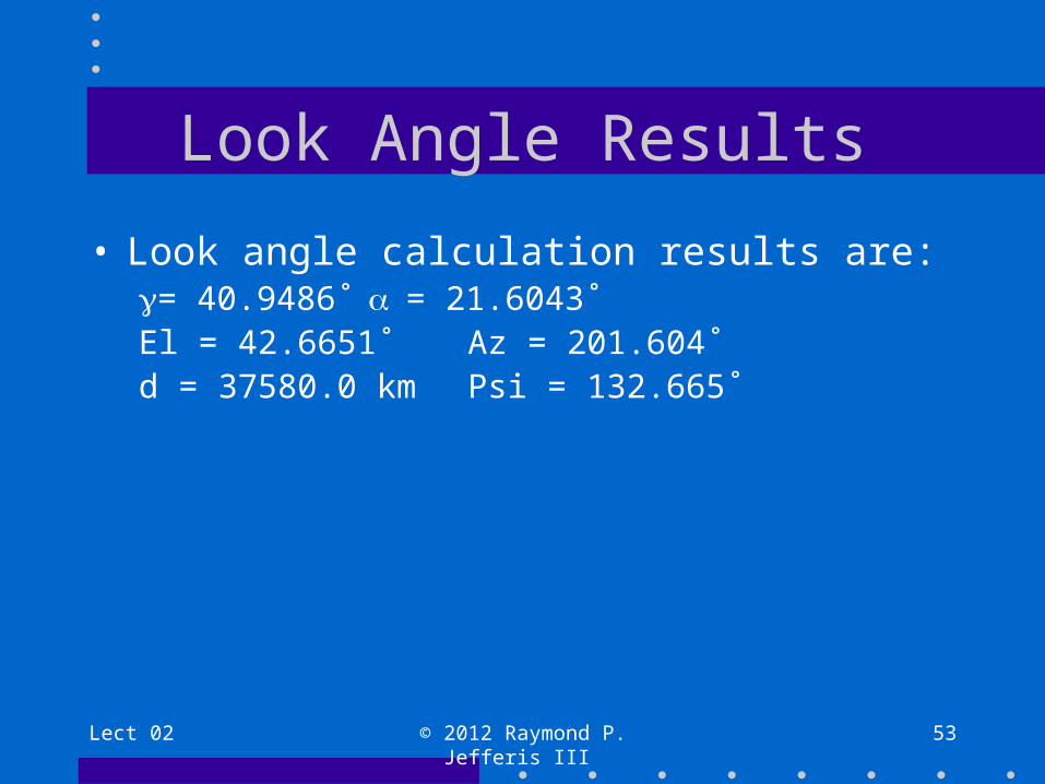
Look Angle Results

• Look angle calculation results are:γ= 40.9486˚ α= 21.6043˚El = 42.6651˚ Az = 201.604˚d = 37580.0 km Psi = 132.665˚


Homework 02B Problem• Earth Station: West Chester, PA

– Latitude: Late = 40° N (+40°)

– Longitude: Lone = 76° W (-76°)

• Satellite: Geosynchronous at 91W– Latitude: Lats = 0° (+0°)

– Longitude: Lons = 91° W (-91°)

• Find range, elevation, and azimuth angle from the earth station to the satellite


Look Angle Results

• Look angle calculation results are:El = 41.1901˚ Az = 157.371˚d = 37689.7 km


Radio Propagation Time Delay

• Radio waves travel at the speed of light:c = 2.99792458 * 108 [m/s]

(Note: The speed of light is slightly less in air.)

• Ground – Geosynchronous Satellite delay:τe-s = d/c

Example:τe-s = 38580.0/c = 0.128689 [s]

(about 129 msec)



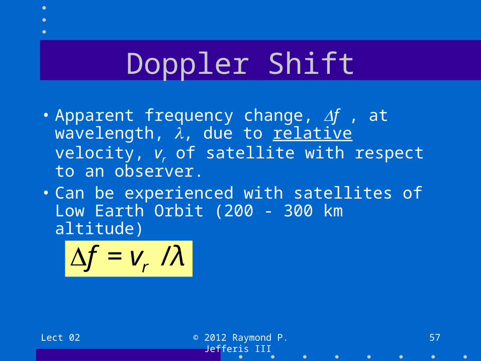
Doppler Shift

• Apparent frequency change, Δf , at wavelength, λ, due to relative velocity, vr of satellite with respect to an observer.

• Can be experienced with satellites of Low Earth Orbit (200 - 300 km altitude)

Δf = vr / λ

Doppler Calculation Terminology

• r = radial distance from center of Earth [km] λwavelength of data link radiation [km]• μ = 3.986004418E5 [km3/s2]



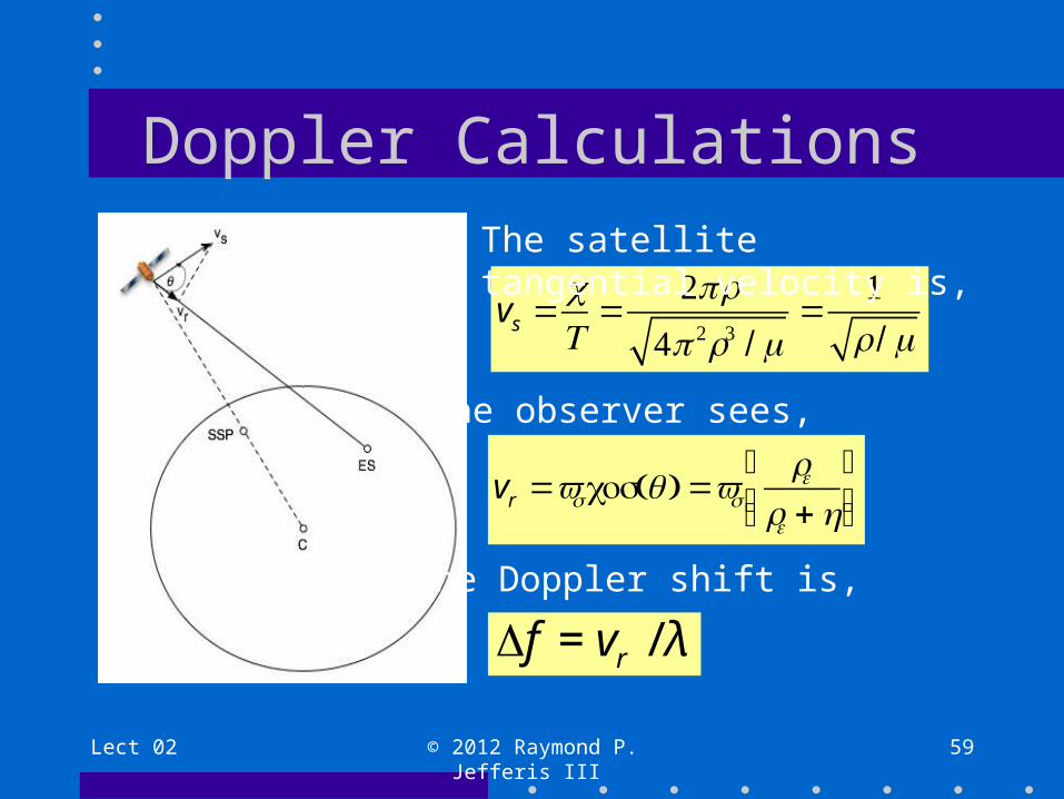
Doppler Calculations

vs =cT

=2πr

4π 2r3 / μ=

1r / μ

The satellite tangential velocity is,

The observer sees,

vr =vs cos θ( ) =vs

rere +h

⎛

⎝⎜⎞

⎠⎟

The Doppler shift is,

Δf = vr / λ


End

lect 02© 2012 raymond p. jefferis iii1 satellite communications orbital calculations orbit...

Documents

orbital eccentricity

major axis lect

axes of ellipse lect

jefferis iii5 slide

minor axis slide

ellipse properties

definition of ellipse

communications slide