502finalpaper_xilun & isaac

An investigation on the effects of demand and supply factors on the producer price of wheat-‐ The Case of Canada (1961-‐2011)

Isaac Jonas 87148145

Xilun (James) Zhang 12328118

Abstract The paper takes a macroeconomic approach in investigating the factors that affect the price path of wheat in Canada. It examines both the demand and the supply factors as drivers of the wheat price variations in Canada over the 1961-‐2011 time frame. List of Acronyms Canadian Wheat Board-‐CWB Gross Domestic Product-‐GDP United States of America-‐US The International Monetary Fund-‐IMF Food and Agricultural Organization-‐FAO Introduction Canada is one of the largest producers and exporters of high quality and most homogeneous

wheat in the world. Most of the Canadian wheat is grown in the Prairie Provinces of Western

Canada of Saskatchewan (46%), Alberta (30%) and Manitoba (14%) 1. Ontario produces about

9% on the Eastern part of Canada; Quebec contributes 1% while the Atlantic produces less than

1% of the total national wheat production in Canada 2.

The top Canadian export wheat is No. 1 CWRS, which is the highest grade Canadian wheat3. The

Canadian Wheat Board (CWB) regulates the wheat market in Canada. The Canadian Wheat

Board was formed in 1935 as a policy instrument to act as the monopoly-‐desk marketing

agency for the Canadian grain 4. The board acted as a policy tool for regulating returns and

stabilizing income, and was based on voluntary participation since its inception until 1943 when

all exporting farmers where required by law to market their wheat grain through the CWB 5.

Although the CWB was repealed by the act of parliament in 2011, the Canadian Wheat Board

1http://publications.gc.ca 2http://www.agr.gc.ca 3http://publications.gc.ca 4 http://www.agr.gc.ca 5 http://laws-‐lois.justice.gc.ca

subsection 3(1) of the Canadian Wheat Board Act mandates the corporation to continue its

operations as Marketing Corporation till 2016.

According to the Canadian Wheat Board Act, the corporation acts as a policy tool by buying,

storing, transferring, selling, shipping or otherwise disposing of grain between the producers

who choose to enter into agreement with the board 6. The Canadian Wheat Board agency

records sales of approximately $3 to $6 billion through the pool accounts system and the

wheat exporters are paid the price reflective of the overall market conditions rather than the

day-‐to-‐day fluctuating prices (ibid). In case of a deficit due to unfavorable world market

prices, the parliament funds the wheat board (ibid).

It operates under the minister of finance’s purview and subject to approval may enter into

banking agreements with the banking sector to help producers of wheat 7.

McCalla (2009) notes exchange rate and Gross Domestic Product drive wheat price. Furthermore, commodity prices move in tandem with broad commodity boom (ibid). Furthermore, McCalla (2009) alludes that the United States dollar is the benchmark for international trade hence the oscillations in the US dollar affect the global commodity markets. Hanke and Ransom cited in McCalla (2009) argue that depreciation of the US dollar makes the commodities cheaper to the rest of the world, driving up the demand and prices. The US dollar appreciation has the opposite effect. Canada is involved in trade of wheat hence the volatility of the US dollar would have an effect in the price of wheat in Canada. Frankel (2013) argues economic uncertainty induces investors to shift from monetary assets to real assets including commodities like wheat. This has secondary impact on the commodity markets (IMF: 2012) McCalla (2009) posits that international commodity markets fluctuate within the rate of supply growth and demand growth. The weather shocks around the globe have an impact on the price path of wheat (ibid). The drought in Australia (2006-‐2008) and the recent California droughts draw down stocks into critical levels. This stimulates speculation (McCalla 2009).

6 http://laws-‐lois.justice.gc.ca 7 http://laws-‐lois.justice.gc.ca

The rising incomes in China and India have also been debatably a major driver of the demand expansion (McCalla 2009). The mismatch between the demand and improved research and development, yield increase and hence improved supply, also cause a shortage and hence price spike (ibid). The graph below shows the relationship between Nominal Wheat Price and GDP over the period of 1961 to 2011.

Fig.1

Fig 2

Fig 3. Figures 1, 2 and 3 show that wheat price is co-‐integrated to per capita GDP of Canada, exchange rate and the world crude prices. The suspects for figure 1 include changes in incomes in Canada due to the economic transformation over time period (McCalla : 2009). The prime suspects of the trend before 1991 could be the volatility in the commodity markets and the crude oil price fluctuations in the 1990s. The oil embargoes and instability in the oil producing

Middle-‐East countries could have influenced the trend pattern. The notable events on the international crude oil markets include but are not limited to the Iranian revolution (1979), the Arab -‐ Israeli war (1967). In 1970s, 1990s, 2000s there was also same oil shock story. However, there are some erratic spikes in the data over time and this intrigued the researchers to investigate the trends econometrically. Research Problem The paper empirically investigates the wheat price fluctuations and reasons behind such pronounced movements over a period of 1961 to 2011. In the paper, a time series analysis with a yearly-‐basis data set is conducted to figure out the dynamics of producer prices for wheat and the incidence of significant fluctuations in wheat price dynamics. A yearly database is used. The data are tested against short-‐term effects on wheat futures markets. A stepwise backwards regression is conducted on the following two models to figure out the optimal regression model.

1. Nominal_Prices = B0 + B1 * GDP_Capita + B2 * Exchange_Rate + B3 * Wheat_Production + B4 * Wheat_Imports + B5 * Wheat_Exports + Error term

2. Log (Nominal_Prices) = B0 + B1 * Log (GDP_Capita) + B2 * Log (Exchange_Rate) + B3 * Log (Wheat_Production) + B4 * Log (Wheat_Imports) + B5 * Log (Wheat_Exports)

Background of the Paper Global Overview of Wheat Market The major wheat exporters are Argentina, Australia, Canada, the EU, Kazakhstan, Russian Federation, Ukraine and the United States (FAO, 2014). On average, (2005/2009) global wheat production was around 637 million tonnes (Mt) with the major producers being the European Union-‐27 (EU-‐27) accounting for 133 Mt or 21% of global production, China contributes 108 Mt, India, 75 Mt, the United States (US) accounts for 58 Mt, Russia with 54 Mt, Canada with 25 Mt or 4% of global production, and Australia with 18 Mt (ibid). Canada is a price taker on the global wheat market. However, it has a niche on high quality and homogeneous wheat quality. The wheat market is thinly traded as most of the product is domestically consumed. Literature Review

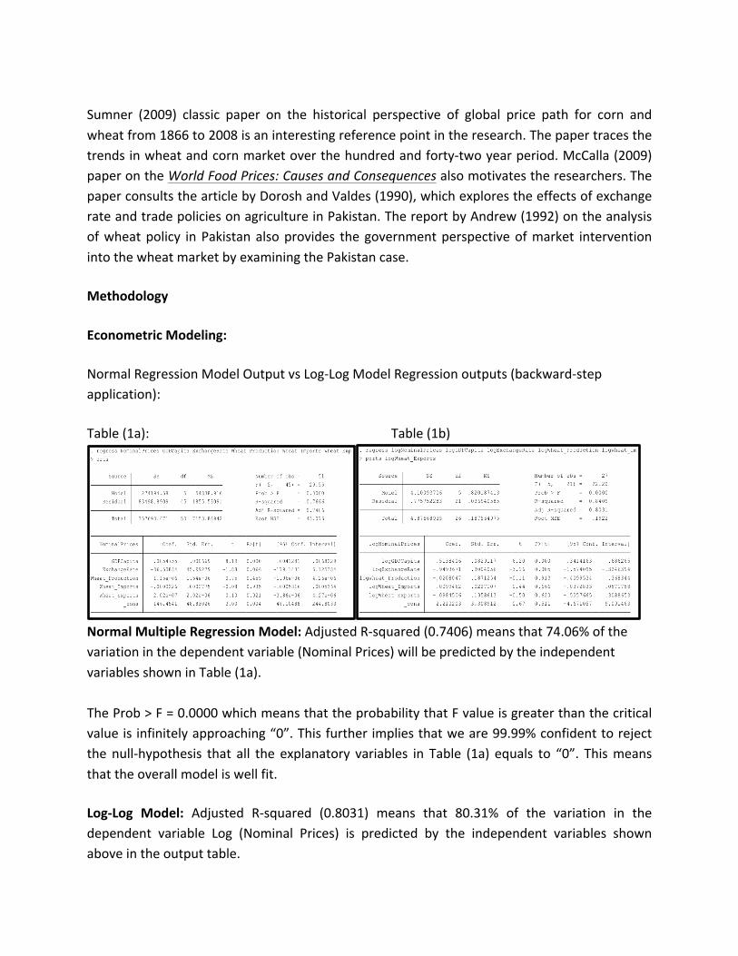
Sumner (2009) classic paper on the historical perspective of global price path for corn and wheat from 1866 to 2008 is an interesting reference point in the research. The paper traces the trends in wheat and corn market over the hundred and forty-‐two year period. McCalla (2009) paper on the World Food Prices: Causes and Consequences also motivates the researchers. The paper consults the article by Dorosh and Valdes (1990), which explores the effects of exchange rate and trade policies on agriculture in Pakistan. The report by Andrew (1992) on the analysis of wheat policy in Pakistan also provides the government perspective of market intervention into the wheat market by examining the Pakistan case. Methodology Econometric Modeling: Normal Regression Model Output vs Log-‐Log Model Regression outputs (backward-‐step application): Table (1a): Table (1b)

Normal Multiple Regression Model: Adjusted R-‐squared (0.7406) means that 74.06% of the variation in the dependent variable (Nominal Prices) will be predicted by the independent variables shown in Table (1a). The Prob > F = 0.0000 which means that the probability that F value is greater than the critical value is infinitely approaching “0”. This further implies that we are 99.99% confident to reject the null-‐hypothesis that all the explanatory variables in Table (1a) equals to “0”. This means that the overall model is well fit. Log-‐Log Model: Adjusted R-‐squared (0.8031) means that 80.31% of the variation in the dependent variable Log (Nominal Prices) is predicted by the independent variables shown above in the output table.

H0: B0=B1=B2=B3=B4=B5=0 H1: at least one is not zero Critical value for 99% of F (5, 21) = 4.04 Given the F test value = 22.20 which is bigger than 4.04 and therefore we reject H0. To conclude, the overall appear to be significant. Backward-‐wise Application: The variable Log (Wheat_Production) appears to be the least significant variable given the P-‐value (0.913) from the Table (1b) and therefore, we drop the explanatory variable LogWheat_Production and get table (2b) shown below: Table (2a) Table (2b)

Normal Multiple Regression Model: The adjusted R-‐square increases from 0.7406 to 0.7462 which implies the explanatory power overall becomes stronger. It means that in this model, 74.62% of the variation of dependent variable will be predicted by the explanatory variables. However, the explanatory variable Wheat_Exports is still statistically insignificant because its P-‐value (0.917) which is much greater 0.05. Therefore, we drop Wheat_Exports and rerun the regression. Log-‐Log Model: The adjusted R-‐square increases from 0.8031 to 0.8119 which implies that the explanatory power overall becomes stronger. It means that in this model, 81.19% of the dependent variable (Log Nominal Prices) is predicted by the independent variables. However, the explanatory variable LogWheat_Imports is still insignificant given its P-‐value 0.662. Therefore, we drop the variable LogWheat_Imports and rerun the multiple regressions for both normal and Log models. We get Table (3a) and Table (3b) as follows:

Table (3a) Table (3b)

Normal Multiple Regression Model: The adjusted R-‐squared increases from 0.7462 to 0.7516 which implies the explanatory power overall becomes stronger. However, the explanatory variable “Wheat_Production” is still statistically insignificant because it has a P-‐value (0.360) much greater than 0.05 (significance level). Therefore, we drop Wheat_Production and rerun the regression. Log-‐Log Model: The adjusted R-‐squared increases from 0.8199 to 0.8223 which implies that the explanatory power overall becomes stronger. However, the explanatory variable Log (Wheat_Exports) still has a P-‐value (0.845) greater than 0.05 that means it is statistically insignificant. Therefore, we drop this variable and rerun the regression and get Table (4b). Table (4a) Table (4b)

Normal Regression Model: the model above still has explanatory variable (ExchangeRate) whose P-‐value (0.056) is greater than 0.05 which implies that this variable is insignificant and therefore we drop the explanatory variable (Exchange Rate) and get table (5a) shown below. Log-‐Log Model: The adjusted R-‐squared increases from 0.8223 to 0.8259 which means that the explanatory power overall becomes stronger since 82.59% of the variation could be explained by the explanatory variables. Now, all the P-‐values are smaller than 0.05 and our optimal Log-‐Log Model will be based on Table (4b):

Log (Nominal_Prices) = -‐0.0819996 + 0.5527993 * Log (GDP_Capita) -‐ 0.7845761 * Log (Exchange_Rate) (0.373603) (0.2573765) (se) Interpretation of the optimal model:

-‐ When GDP per Capita increases by 1%, the Nominal Prices will increase by 0.5527993% holding other variables constant

-‐ When Exchange Rate increases by 1%, the Nominal Prices will decrease by 0.7845761% holding other variables constant

Significance Testing for the remained two explanatory variables (using null-‐hypothesis testing method):

1. It is assumed that the beta coefficients for Log GDP_Capita equals to “0” Ho: B1 = 0 H1: B1 = 0 Using the P-‐value method where alpha = 0.05 P-‐value = 0.000 < 0.05 which means that we could reject the null-‐hypothesis that Log GDP_Capita does not have any relationship with Log Nominal_Prices and they actually have positive relationship with each other.

2. It is assumed that the beta coefficients for Log (ExchangeRate) equals to “0”. This means the Log (Exchange_Rate) does not have any relationship with Log Nominal_Prices. H0: B2 = 0 H1: B2 = 0 Using P-‐value method where alpha = 0.05 P-‐value = 0.000 < 0.05 which means that we could reject the null-‐hypothesis that Log Exchange_Rate does not have any relationship with Log Nominal_Prices and they actually have negative correlation.

Table (5a)

The model above does not have any explanatory variables that are statistically insignificant. In addition, the adjusted R-‐square is still 0.7376 and it provides a decent fit for the model. Specifically, GDP_Capita has a positive coefficient and therefore it has a positive correlation with the dependent variable (Nominal_Prices) Based on Table (5a), we can have the optimal equation: Nominal_Prices = 70.88519 + 0.0054909 * GDP_Capita (0.00046) (se) Interpretation of the model:

-‐ When GDP_Capita increases by 1 unit, Nominal Prices will increase by $0.0054909 holding other variables constant

Significance testing for the only explanatory variables (using null-‐hypothesis testing method)

Hypothetically assuming the beta coefficient for “GDP_Capita” to equal “0” Ho: B1 = 0 H1: B1 = 0 Using the P-‐value method where alpha = 0.05 P-‐value = 0.000 < 0.05 (Significance Level) Thus, we reject the null-‐hypothesis that GDP_Capita does not affect the Nominal Prices and they actually have positive relationship with each other

Covariance Matrix:

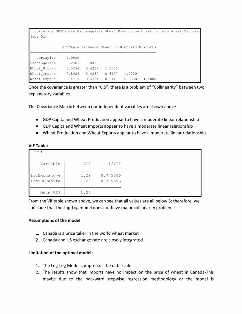
Once the covariance is greater than “0.5”, there is a problem of “Collinearity” between two explanatory variables. The Covariance Matrix between our independent variables are shown above

● GDP Capita and Wheat Production appear to have a moderate linear relationship ● GDP Capita and Wheat Imports appear to have a moderate linear relationship ● Wheat Production and Wheat Exports appear to have a moderate linear relationship

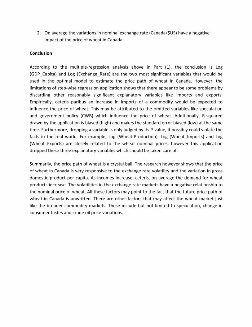
VIF Table:

From the Vif table shown above, we can see that all values are all below 5; therefore, we conclude that the Log-‐Log model does not have major collinearity problems. Assumptions of the model

1. Canada is a price taker in the world wheat market 2. Canada and US exchange rate are closely integrated

Limitation of the optimal model:

1. The Log-‐Log Model compresses the data scale 2. The results show that imports have no impact on the price of wheat in Canada-‐This

maybe due to the backward stepwise regression methodology or the model is

misspecified. This may be a result of other omitted qualitative variables like speculation. This could be captured by using a binary probability.

3. By using backward-‐step application, there are two optimal models generated from normal and Log-‐Log Models. The normal model has only one explanatory variable – GDP_Capita while the log-‐log model has two significant explanatory variables that are respectively Log (GDP_Capita) and Log (Exchange_Rate). However, in fact, normal regression should not drop the explanatory variables “Wheat_Exports”, “Wheat_Imports”, “Wheat_Production” and “Exchange Rate” because they are correlated with the “Nominal Prices”. The Log-‐Log model should not drop “Log (Wheat_Imports)”, “Log (Wheat_Exports)” and “Log (Wheat_Production)” because they are related to “Log (Nominal_Prices)” as its dependent variable. Therefore, based on the aforementioned econometric observations, there exists a limit in our model. Testing the model with common sense against real world observations can rectify this.

Heteroskedasticity and Normality Testing with Residual and Normality Plots Log (Nominal Price) vs Log (GDP_Capita)

The residual plot does not distributed randomly around “0” which implies presence of heteroskedasticity. The Normality Plot forms a fairly straight line that means the data are normally distributed. Log(Nominal Price) vs Log(Exchange Rate)

The residual plot does not distributed randomly around “0” which implies there is heteroskedasticity. The Normality Plot does not form a straight line that means the data are not normally distributed. Log(Nominal Price) vs Log(Wheat Production)

The residual plot does not distributed randomly around “0” which implies presence of heteroskedasticity. The Normality Plot forms a relatively straight line that means the data are fairly normally distributed. Log (Nominal Price) vs Log (Wheat Imports)

The residual plot is not distributed evenly around “0” which implies presence of heteroskedasticity. The Normality Plot does not form a straight line that means the data are not normally distributed. Log (Nominal Price) vs Log (Wheat Exports)

The residual plot does not distributed randomly around “0” which implies heteroskedasticity. The Normality Plot does not form a straight line that means the data are not normally distributed. Comparison between Normal and Log-‐Log Model: The normal regression model and Log-‐Log Model, we will choose the Log-‐Log model which transformed a variable by taking the natural logarithm. Our decision could be supported in terms of three aspects:

1. With a Log-‐Log Model, the model fit will be improved. The data for all residuals are not normally distributed in the normal model, by taking the logarithm of the skewed

variables, we could make the variables more normally distributed as the above normality plots show.

2. By logging one or more variables in the model, model interpretation will be more convenient. Once both dependent variable and independent variables are logged, the beta coefficients (B) will be converted into elasticity and the interpretation of the model will go as follows: a 1% increase in a X variable will cause a ceteris paribus B% change in Y variable on average.

3. R-‐square of Log-‐Log Model is greater than that of Normal Regression Model. For example, by comparing Table (1a) and Table (1b) with all 5 explanatory variables, we figure out that the adjusted R-‐square (0.8031) of Log-‐Log Model is greater than that of Normal Regression Model (0.7406) which means that the explanatory power overall is higher in the Log-‐Log Model.

Results By using the time series data for the period between 1961 and 2011 as well as the backward step, the optimal regression model is: Log (Nominal_Prices) = -‐0.0819996 + 0.5527993 * Log (GDP_Capita) -‐ 0.7845761 * Log (Exchange_Rate) Data Sources

1. GDP/capita. The Gross Domestic Product is taken from the World Bank database. To get per Capita GDP, the GDP is divided with the population across each respective year. (http://databank.worldbank.org/data/home.aspx)

2. Imports. The trade data is taken from the Food and Agricultural Organization (FAO). (http://faostat3.fao.org/download/T/*/E)

3. Production (http://faostat3.fao.org/download/T/*/E) 4. Canada Wheat price-‐Source. The data is extracted from the FAO website. 5. Exchange rate. The exchange rate were taken from the University of British of Columbia

Pacific Exchange rate Service website (http://fx.sauder.ubc.ca/data.html) Recommendations

1. On average, the GDP/capita has a positive effect in explaining price of wheat in Canada

2. On average the variations in nominal exchange rate (Canada/$US) have a negative impact of the price of wheat in Canada

Conclusion According to the multiple-‐regression analysis above in Part (1), the conclusion is Log (GDP_Capita) and Log (Exchange_Rate) are the two most significant variables that would be used in the optimal model to estimate the price path of wheat in Canada. However, the limitations of step-‐wise regression application shows that there appear to be some problems by discarding other reasonably significant explanatory variables like imports and exports. Empirically, ceteris paribus an increase in imports of a commodity would be expected to influence the price of wheat. This may be attributed to the omitted variables like speculation and government policy (CWB) which influence the price of wheat. Additionally, R-‐squared drawn by the application is biased (high) and makes the standard error biased (low) at the same time. Furthermore, dropping a variable is only judged by its P-‐value, it possibly could violate the facts in the real world. For example, Log (Wheat-‐Production), Log (Wheat_Imports) and Log (Wheat_Exports) are closely related to the wheat nominal prices, however this application dropped these three explanatory variables which should be taken care of. Summarily, the price path of wheat is a crystal ball. The research however shows that the price of wheat in Canada is very responsive to the exchange rate volatility and the variation in gross domestic product per capita. As incomes increase, ceteris, on average the demand for wheat products increase. The volatilities in the exchange rate markets have a negative relationship to the nominal price of wheat. All these factors may point to the fact that the future price path of wheat in Canada is unwritten. There are other factors that may affect the wheat market just like the broader commodity markets. These include but not limited to speculation, change in consumer tastes and crude oil price variations.

References 1. Branch, Legislative Services. “Consolidated Federal Laws of Canada, Canada Grain Act,”

May 29, 2014. http://laws-‐lois.justice.gc.ca/eng/acts/G-‐10/page-‐1.html#h-‐1. 2. Government of Canada, Canadian Grain Commission. “Canadian Wheat -‐ Official Grains

of Canada.” Fact sheet, November 14, 2008. 3. Dorosh, Paul Anthony, and Alberto Valdés. Effects of Exchange Rate and Trade Policies

on Agriculture in Pakistan. Intl Food Policy Res Inst, 1990. 4. McCalla, Alex F. “World Food Prices: Causes and Consequences.” Canadian Journal of

Agricultural Economics/Revue Canadienne D’agroeconomie 57, no. 1 (March 1, 2009): 23–34. Doi: 10.1111/j.1744-‐7976.2008.01136.x.

5. Sumner, Daniel A. “Recent Commodity Price Movements in Historical Perspective.” American Journal of Agricultural Economics 91, no. 5 (December 1, 2009): 1250–56.

6. http://www.imf.org/external/np/seminars/eng/2012/commodity/pdf/frankel.pdf.Acces

sed online.6 December, 2014

7. http://www.agr.gc.ca/ Accessed online.6 December,2014

8. http://laws-‐lois.justice.gc.ca/eng/acts/C-‐24.2/page-‐2.html.Accessed online.6 December,

2014

9. http://fx.sauder.ubc.ca/data.html.Accessed online.6 December, 2014

10. http://databank.worldbank.org/data/home.aspx.6 December, 2014

11. http://faostat3.fao.org/download/T/*/E.6 December, 2014

12. http://www.grainscanada.gc.ca/statistics-‐statistiques/cge-‐ecg/cgem-‐mecg-‐eng.htm. 13. Jayne, Thomas S., and Robert J. Myers. “The Effect of Risk on Price Levels and Margins in

International Wheat Markets.” Review of Agricultural Economics 16, no. 1 (January 1, 1994): 63–73. Doi: 10.2307/1349521.

14. http://www.fao.org/worldfoodsituation/csdb/en/. Accessed online. November 9,2014. 15. http://faostat.fao.org/site/703/DesktopDefault.aspx? PageID=703#ancor. Accessed

online. November 11,2014. 16. Canada, Agriculture and Agri-‐Food Canada; Government of. Wheat Sector Profile -‐ Part

One: Overview (November 2010). Report, September 27, 20 http://publications.gc.ca/Collection-‐R/LoPBdP/modules/prb98-‐2-‐grain/wheatboard-‐e.htm 13. http://publications.gc.ca/Collection-‐R/LoPBdP/modules/prb98-‐2-‐grain/wheatboard-‐e.htm. Accessed online, November 2014.

17. http://laws-‐lois.justice.gc.ca/eng/acts/C-‐24.2/page-‐2.html. 18. Government of Canada, Statistics Canada. “The Daily — Production of Principal Field

Crops, July 2014,” August 21, 2014. 19. http://www.indexmundi.com/commodities/?commodity=rice. 20. http://www.wtrg.com/prices.htm. Accessed online. November 6,2014

21. http://inflationdata.com/Inflation/Inflation_Rate/Historical_Oil_Prices_Chart.asp. Accessed online. November 6,2014

502finalpaper_xilun & isaac

Documents