4 fsm-design 4dsp using matlab - oth regensburg · pdf filethis tutorial is intended to be...

lektronikabor

Course and Laboratory on Electronic Design Automation

RED / PRED

FSM Design for Digital Signal Processing Using Matlab

Prof. Dr. Martin J. W. Schubert

Electronics Laboratory

Regensburg University of Applied Sciences

Regensburg

M. Schubert RE2 / PRE2 FSM Design for DSP Using Matlab Regensburg Univ. of Appl. Sciences

- 2 -

Abstract. This tutorial is intended to be both an advanced introduction to Matlab and a guide how to check the functionality of a digital finite state machine (FSM) design. Examples are taken from the field of digital signal processing (DSP). An understanding of the theoretical background of DSP with respect to the used ΔΣ modulator and filter examples are not required.

1 Introduction It may be very helpful in several situations to check a digital design on a high level which is easy to implement before coding details using a hardware description language like VHDL or Verilog. This guide demonstrates how to model a finite state machine (FSM) using Matlab. We employ Matlab rather than C due to the better graphical support and toolboxes within Matlab. Some chapters use the fdatool (filter design & analysis) of Matlab. The reader may jump over this chapters without problems to continue. Matlab is not free. Open source freeware with same functionality (except some toolboxes) can be obtained from octave [3]: Homepage: whttp://www.octave.org or http://www.gnu.org/software/octave/ Windows installer: http://octave.sourceforge.net/ Graphical options: gnuplot or jhandles. The latter is based on Java and more similar to Matlab, gnuplot is faster (and some people think that it makes more beautiful graphics). The Matlab FSM models presented below run on plain Matlab or its open source counterparts Octave [3] and Scilab [4]. In this tutorial Matlab was preferred to C due to the ease of use and its graphical features. The organization of this document is as follows:

Chapter 1 introduction,

Chapter 2 uses basic Matlab commands illustrating a counter as finite state machine (FSM).

Chapter 3 illustrates how to obtain a self-made impulse response for time-discrete low-, band- and high-passes.

Chapter 4 demonstrates how to write self-made Bode diagrams in s and z.

Chapter 5 introduces Matlab supported LTI models in s and z.

Chapter 6 models the effect of finite bit-vector lengths.

Chapter 7 introduces FSM design of modulators and

Chapter 8 of digital filters for demodulation.

Chapter 9 illustrates the us of Matlab’s Filter Design & Analysis Tool (fdatool),

Chapter 10 draws relevant conclusion,

Chapter 11 offers some references.


- 3 -

2 LTI Systems 2.1 Matlab’s Linear and Time-Invariant (LTI) Systems

2.1.1 Matlab LTI System Basics

Listing 2.1.1: Matlab LTI System Fundamentals

% Matlab LTI System Basics: % Create transfer functions using tf and zpk: A0 = 10; D=1/2; f0=1e4; w0=2*pi*f0; a0=A0*w0^2; b0=w0^2; b1=2*D*w0; b2=1; TFs = tf([a0], [b2 b1 b0]) % transfer function in s-domain TFszpk = zpk([1], [-0.5 -0.6], 3) % zero-pole-konstant in s-domain fs=1e5; Ts=1/fs; % sampling rate and interval TFz = tf([3 -3], [1 2 3], Ts) % transfer function in z-domain TFzzpk = zpk([1], [-0.5 -0.6], 3, -1) % zpk in z-domain, Ts unspecified Complete the following Matlab-statement such, that we get the Matlab echo printed below. (See next page for solutions.) » TF_s = ................................................... Transfer function: s + 10 ----------------------------- s^4 + 4 s^3 + 6 s^2 + 4 s + 1 Complete the following Matlab-statement such, that we get the Matlab echo printed below. » TF_z = ................................................... Transfer function: z + 10 ----------------------------- z^4 + 4 z^3 + 6 z^2 + 4 z + 1 Sampling time: 0.001 2.1.2 Matlab LTI System Type Conversion

Listing 2.1.2: Matlab LTI System Type Conversion. Run listing 2.1.1 before

% Matlab LTI System Model Type Conversion. Run LTI_Basics.m before! % Matlab LTI System Model Type Conversion. Run LTI_Basics.m before! TFs_from_TFszpk = tf(TFszpk) % zero-pole-constant to polynomial in s TFszpk_from_TFs = zpk(TFs) % polynomial to zero-pole-constant in s TFz_from_TFszpk = tf(TFzzpk) % zero-pole-constant to polynomial in z TFzzpk_from_TFz = zpk(TFz) % polynomial to zero-pole-constant in z Listing 2.1.2 converts the model from polynomial to zer/pole/constand representation and vice versa. It requires that you run listing 2.1.1 before.


- 4 -

2.1.3 Matlab LTI System Domain Conversion

Listing 2.1.3: Matlab LTI System Domain Conversion. Run listing 2.1.1 before

% Matlab LTI System Model Domain Conversion. Run LTI_Basics.m before! fs=1e5, Ts=1/fs; % sampling rate and interval TFs % display TFs TFz = c2d(TFs,Ts) % s to z TFs_from_TFz = d2c(TFz) % z to s Listing 2.1.3 converts the model from time-continuous to time-discrete (c2d) domain and vice versa (d2c). 2.1.4 Matlab LTI System Graphics

Listing 2.1.4: Matlab LTI Graphics. Run listings 2.1.1 and 2.1.3 before

% LTI_graphics. Run LTI_Basics.m and LTI_DomainConversion.m before! if not(exist('TFHs')); figure(1); impulse(TFs,TFz); % grid on; figure(2); step(TFs,TFz); grid on; figure(3); bode(TFs,TFz); grid on; bo = bodeoptions; bo.FreqUnits = 'Hz'; figure(4); bodeplot(TFs,TFz,bo); grid on; else figure(1); impulse(TFs,TFz,TFHz); % grid on; figure(2); step(TFs,TFz,TFHz); grid on; figure(3); bode(TFs,TFz,TFHz); grid on; bo = bodeoptions; bo.FreqUnits = 'Hz'; bo.Ylim=[-60 30]; figure(4); bodeplot(TFs,TFz,TFHz,bo); grid on; end; Listing 2.1.4 illustrates how to generate some graphics. Commands impulse(…) and delivers impulse responses of the lited LTI models. Commands step(…) and delivers step responses of the lited LTI models. Command bode(…) creates easily a Bode diagram but cannot be modified. Command bodeplot(…) is identical to bode(…) when used without options, but it allows

to modify the default settings. In the example we display the abscissa in Hz rather than rad/s. Type help bodeoptions to or simply the variable name bo after running the code above to see the complete record of options.

Solution for LTI - Models in Matlab Complete the following Matlab-statement such, that we get the Matlab echo printed below. » TF_s = tf([1 10], [1 4 6 4 1]) Transfer function: s + 10 ----------------------------- s^4 + 4 s^3 + 6 s^2 + 4 s + 1 Complete the following Matlab-statement such, that we get the Matlab echo printed below. » TF_z = tf([1 10], [1 4 6 4 1], 0.001) Transfer function: z + 10 ----------------------------- z^4 + 4 z^3 + 6 z^2 + 4 z + 1 Sampling time: 0.001


- 5 -

2.2 Selfmade Notation of LTI Systems To get better access to the LTI system coeffients and manipulate them the author uses for didactical reasons an own model of LTI systems consisting of a 1xN matrix, wehere N is SystemOrder+1. Listing 2.2.1: Matlab LTI Graphics. Run listings 2.1.1 and 2.1.3 before

% Basics of Selfmade LTI models A0 = 10; D=1/2; f0=1e4; w0=2*pi*f0; a0=A0*w0^2; a1=0, a2=0; b0=w0^2; b1=2*D*w0; b2=1; fs=1e5,; Ts=1/fs; % sampling rate and period, respectively Hs = [[a0 a1 a2]; [b0 b1 b2]] % selfmade TF matrix model in s-domain Hz = f_c2d_bilin_order2(Hs,Ts) % selfmade TF matrix model in z-domain TFHs = tf(f_h(Hs(1,:)), f_h(Hs(2,:))) TFHz = tf(Hz(1,:),Hz(2,:),Ts) Listing 2.2.2: Matlab code to flip horizontal matrix M

% flip horizontal matrix M function M_flipped_horizontal=f_h(M) ncols=size(M,2); for col=1:ncols; M_flipped_horizontal(:,col) = M(:,ncols+1-col); end; Listing 2.2.3: Matlab code for bilinear transformation s->z of a biquad model in s

% Selfmade continuous to discrete translation for 2nd order models function Hz = f_c2d_bilin_order2(Hs,Ts) % fs2=2/Ts; a0=Hs(1,1); a1=Hs(1,2); a2=Hs(1,3); if size(Hs,1)==1; b0=1; b1=0; b2=0; else b0=Hs(2,1); b1=Hs(2,2); b2=Hs(2,3); end; as0=a0; as1=a1*fs2; as2=a2*fs2*fs2; bs0=b0; bs1=b1*fs2; bs2=b2*fs2*fs2; cs0=bs0+bs1+bs2; cs1=2*(bs0-bs2); cs2=bs0-bs1+bs2; ds0=as0+as1+as2; ds1=2*(as0-as2); ds2=as0-as1+as2; Hz = [[ds0 ds1 ds2];[cs0 cs1 cs2]]; if cs0~=1; Hz=Hz/cs0; end; In our didactical models we use 2xN with N=order+1 matrixes H, with upper row H(1,:) being used as numerator and lower row H(2,:) as denominator

order

k

k

order

k

k

order

k

kk

order

k

kk

skH

skH

sb

sasH

0

0

0

0

)1,2(

)1,1()(


- 6 -

Note that in our model polynomial coefficients rise while in the Matlab modelt he fall from left to right. Therefore we need the flip-horizonal function f_h(…). H(2,1)==1 is used as indicator that the system is time-discrete. As the author uses z-1 while Matlab uses z the order of coefficients is consistent with Matlab and needs not to be flipped.

order

k

k

order

k

k

order

k

korder

order

k

korder

order

k

kk

order

k

kk

zkH

zkH

zkH

zkH

zc

zdzH

0

0

0

0

0

0

)1,2(

)1,1(

)1,2(

)1,1()(

If H is a vector with one row only, then the 2nd row is assumed to be [1 0… 0], and the system is consequently a time-discrete FIR filter. Note that Matlab-Simulink offers both time-discre models in z and in z-1, whereas the first is typically used for control tasks and the latter by signal processing engineers. Multiplicatoin with z is sampled in the future and multiplication with z-1 correspons to samples in the past. From a modeling point of view a denominator [1] with z-1 corresponds to [1 0...0] a with z.


- 7 -

3 Basic FSM Design Considerations Using HDLs 3.1 General Considerations Well recognized top-level hardware description languages (HDL) are System C/C++ [1] and the Matlab/Simulink HDL Coder toolbox [2]. System C/C++ [1] can be simulated with any C/C++ compiler. Additional tools are

required (i) to present the results graphical and (ii) to translate System C/C++ to synthesizable VHDL or Verilog code.

The Matlab/Simulink HDL Coder toolbox [2] has to be afforded and needs some time to get familiar with.

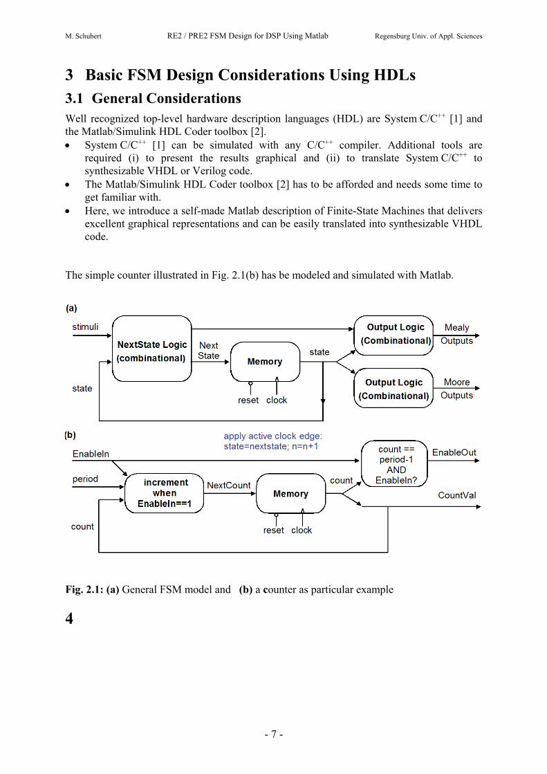
Here, we introduce a self-made Matlab description of Finite-State Machines that delivers excellent graphical representations and can be easily translated into synthesizable VHDL code.

The simple counter illustrated in Fig. 2.1(b) has be modeled and simulated with Matlab.

Fig. 2.1: (a) General FSM model and (b) a counter as particular example

4


- 8 -

Exercise: Identify in Fig. 2.1(b) … (solutions see end of this page) Stimuli: .............................................. NextState: .............................................. State: .............................................. NextState Logic: .............................................. Mealy Outputs: .............................................. Moore Outputs: .............................................. Output Logic Mealy: .............................................. Output Logic Moore: .............................................. Which signals must be initialized? ..................................... Apply active clock edge outside nextstate function, long form form: for n=1:length(stimuli); [y(n),nextstate] = f_nextstate_logic(stimuli(n),state); state = nextstate; end;

Apply active clock edge outside nextstate function, short form form: for n=1:length(stim); [y(n),state]=f_nextstate_logic(stim(n),state); end;

Listing 2.1: Basic Principle to write a FSM module with Matlab (filename=function_name)

function [y,nextstate] = f_nextstate_logic(stimuli,state) % initializations if not(exist('state')); state = zeros(1,...); for n=1:length(stimuli); % Loop until length(time_axis) == legth(stimuli) % nextstate logic nextstate = f_(stimuli,state); % output logic y(n) = f(stimuli,state); % apply active clock edge, required for situation n < length(x) state = nextstate; end; % end Loop over time axis Solutions: Solutions: Stimuli: ...EnableIn, period .......................................... NextState: ...NextCount ................................................. State: ...count ..................................................... NextState Logic: ...increment when enable =1................................... Moore Outputs: ...CountVal .................................................. Mealy Outputs: ...EnableOut ................................................. Output Logic Moore: ...CountVal = count .......................................... Output Logic Mealy: ...EnableOut = EnableIn & (count==period-1) .................. Which signals MUST be initialized how? ...all stimuli


- 9 -

4.1 FSM Model of a Counter with Matlab

4.1.1 Counter Module Description

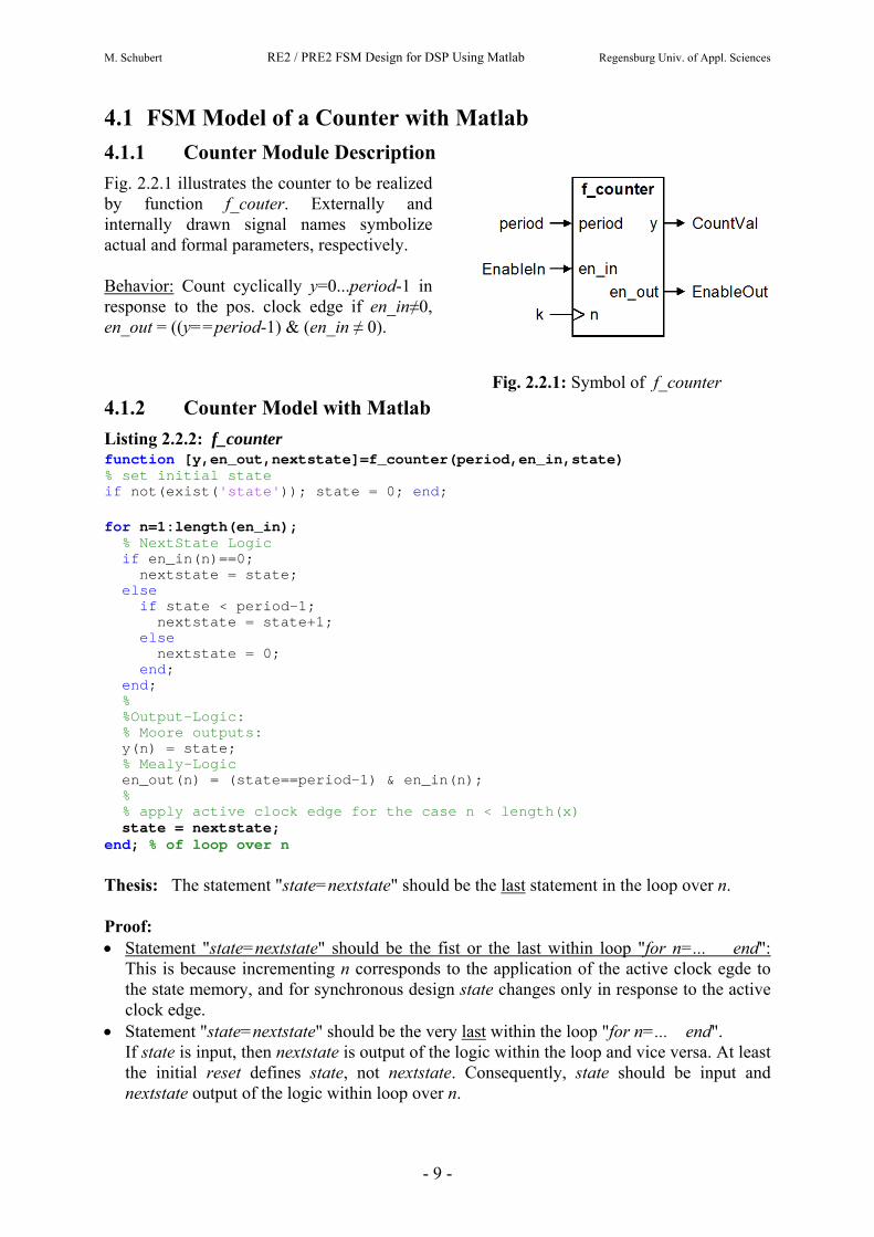
Fig. 2.2.1 illustrates the counter to be realized by function f_couter. Externally and internally drawn signal names symbolize actual and formal parameters, respectively. Behavior: Count cyclically y=0...period-1 in response to the pos. clock edge if en_in≠0, en_out = ((y==period-1) & (en_in ≠ 0).

Fig. 2.2.1: Symbol of f_counter

4.1.2 Counter Model with Matlab

Listing 2.2.2: f_counter function [y,en_out,nextstate]=f_counter(period,en_in,state) % set initial state if not(exist('state')); state = 0; end; for n=1:length(en_in); % NextState Logic if en_in(n)==0; nextstate = state; else if state < period-1; nextstate = state+1; else nextstate = 0; end; end; % %Output-Logic: % Moore outputs: y(n) = state; % Mealy-Logic en_out(n) = (state==period-1) & en_in(n); % % apply active clock edge for the case n < length(x) state = nextstate; end; % of loop over n Thesis: The statement "state=nextstate" should be the last statement in the loop over n. Proof: Statement "state=nextstate" should be the fist or the last within loop "for n=... end":

This is because incrementing n corresponds to the application of the active clock egde to the state memory, and for synchronous design state changes only in response to the active clock edge.

Statement "state=nextstate" should be the very last within the loop "for n=... end". If state is input, then nextstate is output of the logic within the loop and vice versa. At least the initial reset defines state, not nextstate. Consequently, state should be input and nextstate output of the logic within loop over n.


- 10 -

4.1.3 Double Mode Testbench tb_counter

Listing 2.2.3: tb_counter % Testbench tb_counter % % initializations NoS = 51; % Number of Samples period = 16; % stimuli: count period length EnableIn = logical(ones(1,NoS)); % stimuli: input enable EnableIn(25:36) = logical(zeros(1,12)); % stimuli: input enable % % Index 2: work off complete time axis within submodule f_counter [y2,EnableOut2] = f_counter(period,EnableIn); % % Index 1: work through abscissa sample by sample over loop index k state=0; for k=1:NoS; [y1(k),EnableOut1(k),nextstate] = f_counter(period,EnableIn(k),state); % apply active clock edge state = nextstate; end; % time loop over k % % Graphical Postprocessing figure(223) t=0:NoS-1; plot(t,EnableIn+1,'k',t,y1,'b',t,EnableOut2,'g'); hold on; stem(t,EnableIn+1,'k'); stem(t,y1,'b'); stem(t,EnableOut1,'g'); hold off; title('cycle based counter model') xlabel('clock cycle'); ylabel('en_i_n_,_b_l_k, en_o_u_t_,_g_r_n, y_b_l_u');

Listing 2.2.3 details testbench tb_counter producing Fig. 2.2.3: Sim1: The first use of f_counter is a single statement and EnableIn is a vector causing y1, EnableOut1 to be vectors of same length. There is neiter a need for input parameter state nor output nextstate. Sim2: In the second use of f_counter input EnableIn(k) is a scalar value producing scalar outputs y2(k) and EnableOut2(k). The application of the active clock edge is done with the statement "state = nextstate" in the testbench, so that function f_counter needs input parameter state and output nextstate.

Fig. 2.2.3: Different counter simulations: Circles: External loop for "k=... end" of testbench tb_counter works off abscissa. Solid lines: The internal loop for "n=... end" of f_counter works off the abscissa.

The simulation is done with two methods: 1. Apply active clock edge outside the function which evaluates ony the nextstate logic.

Indicated by circles in Fig. 2.2.3. 2. Apply active clock edge within the function, indicated by solid lines in Fig. 2.2.3,

achieved by passing a vector x to function f_counter instead of single samles x(n). The 2nd method is more comfortable to use, but for modules being a part of a feedback loop we need this sample-by-sample processing.


- 11 -

4.2 Exercise: FSM Model of a Filter with Matlab

4.2.1 Counter Module Description

Fig. 2.3.1 illustrates the filter structure to be realized be the function f_filter_canon1. Uppercase and lowercase signal names symbolize frequency and time domain views, respectively. Time domain equation to be solved: y(n) = d0ꞏx(n) + d1ꞏx(n-1) + d2ꞏx(n-2) + - c1ꞏy(n-1) - c2ꞏy(n-2) Frequency domain behavior:

1 20 1 2

1 21 2

( )( )

( ) 1

d d z d zY zH z

X z c z c z

Fig. 2.3.1: Schematics of module

f_filter_canon1_order2 Exercise: Identify in Fig. 2.3.1 … (solutions see end of this page) Stimuli: .............................................. NextState: .............................................. State: .............................................. NextState Logic: .............................................. .............................................. Mealy Outputs: .............................................. Moore Outputs: .............................................. Output Logic Mealy: .............................................. Output Logic Moore: .............................................. Which signals must be initialized? ..................................... Stimuli: .. x(n), initial state ....................... NextState: .. ns1, ns2 .................................. State: .. s1, s2 ................................... NextState Logic: .. ns1 = d1 x(n) – c1 y(n) + s2 ................ .. ns2 = d2 x(n) – c2 y(n) .................... Mealy Outputs: .. y(n) ..................................... Moore Outputs: .. <none> ................................... Output Logic Mealy: .. y(n) = d0x(n) + s1 , ....................... .. nextstate = [ns1, ns2] .................... Output Logic Moore: .............................................. Which signals must be initialized? .. all stimuli and state ....................


- 12 -

4.2.2 Matlab Model of f_filter_canon1_order2

f_filter_canon1_order2 has to be designed as Matlab function realizing the second order infinite impulse response (IIR) filter in canonical direct structure as illustrated in Fig. 2.3.1. Input paramters:

Hz: required: 2x3 array holding coefficients: 0 1 2

0 1 2

d d dHz

c c c

x: required: 1xNoS array holding vector x(n): 1 2 3 ... NoSx x x x x , with NoS ≥ 1

state: optional: 1x2 array holding state vector: 1 2x s s , default: [0 0].

Output paramters: y: 1 x NoS array holding vector y(n): 1 2 3 ... NoSy y y y y , same length as x.

nextstate: 1 x 2 array holding next-state vector: 1 2nextstate ns ns

Listing 2.3.2: f_filter_canon1_order2 (solution on next page) function [y,nextstate] = f_filter_canon1_order2(Hz,x,state) assert(size(Hz,1)==2 & size(Hz,2)==3,'input Hz must have size 2 x 3'); if Hz(2,1)~=1; Hz = Hz/Hz(2,1); end; % enforce c0==1. if not(exist('state')); state=zeros(1,2); end; % set default for state d0=Hz(1,1); d=Hz(1,2:end); % numerator coefficients c0=1; c=Hz(2,2:end); % denominator coefficients % % loop over time axis for n=1:length(x); .............................................................. .............................................................. .............................................................. .............................................................. end; % of loop over n Some explanations: 1. The first line declares the function and its interface paramteres. 2. “Assert” stands for “make sure”. The line assert(logic_expression,error_message) stops

the program and prints string error_message when logic_expression is false. 3. Coefficient c0 corresponding to Hz(2,1) must be 1, otherwise we’ll divide Hz by c0.This

delivers an error message when c0=0. 4. Input vector state is optional. If no input state is given it defaults to [0 0]. 5. The polynomial coefficients d0, d1, d2 correspond to Hz[1,1:3]. We take d0, d1, d2 over

from Hz[1,1:3] such, that d0=d0, d(1)=d1, d(2)=d2. 6. The polynomial indices c0, c1, c2 correspond to Hz[2,1:3]. We take c0, c1, c2 over such,

that c0=c0 (which is not really necessary as c0=1) and c(1)=c1, c(2)=c2.


- 13 -

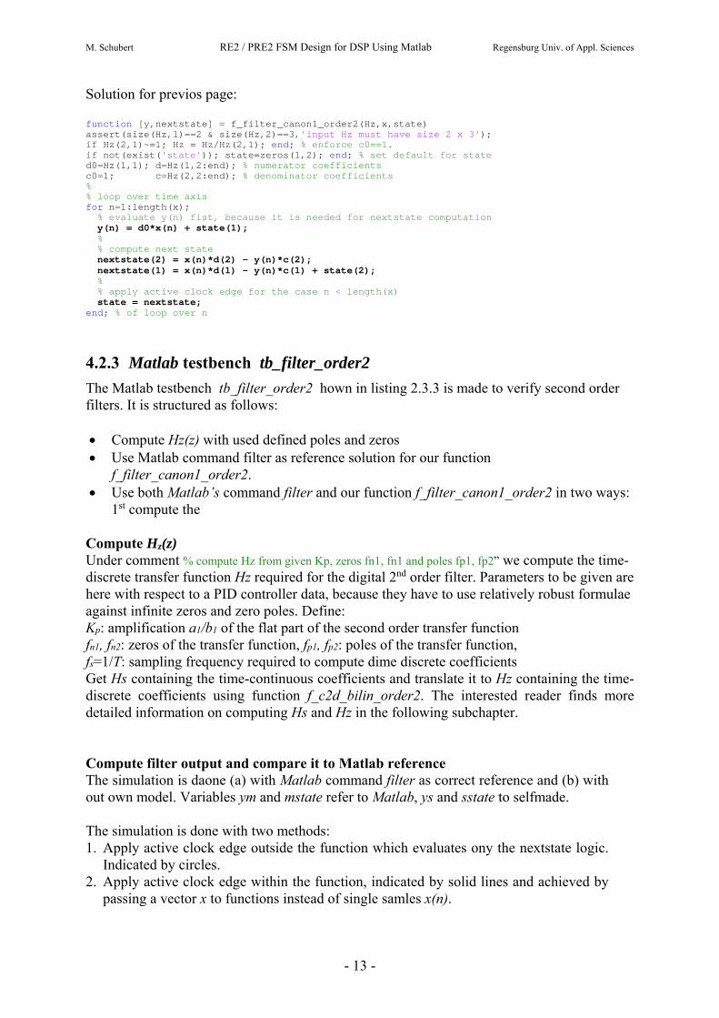
Solution for previos page: function [y,nextstate] = f_filter_canon1_order2(Hz,x,state) assert(size(Hz,1)==2 & size(Hz,2)==3,'input Hz must have size 2 x 3'); if Hz(2,1)~=1; Hz = Hz/Hz(2,1); end; % enforce c0==1. if not(exist('state')); state=zeros(1,2); end; % set default for state d0=Hz(1,1); d=Hz(1,2:end); % numerator coefficients c0=1; c=Hz(2,2:end); % denominator coefficients % % loop over time axis for n=1:length(x); % evaluate y(n) fist, because it is needed for nextstate computation y(n) = d0*x(n) + state(1); % % compute next state nextstate(2) = x(n)*d(2) - y(n)*c(2); nextstate(1) = x(n)*d(1) - y(n)*c(1) + state(2); % % apply active clock edge for the case n < length(x) state = nextstate; end; % of loop over n

4.2.3 Matlab testbench tb_filter_order2

The Matlab testbench tb_filter_order2 hown in listing 2.3.3 is made to verify second order filters. It is structured as follows: Compute Hz(z) with used defined poles and zeros Use Matlab command filter as reference solution for our function

f_filter_canon1_order2. Use both Matlab’s command filter and our function f_filter_canon1_order2 in two ways:

1st compute the Compute Hz(z) Under comment % compute Hz from given Kp, zeros fn1, fn1 and poles fp1, fp2” we compute the time-discrete transfer function Hz required for the digital 2nd order filter. Parameters to be given are here with respect to a PID controller data, because they have to use relatively robust formulae against infinite zeros and zero poles. Define: Kp: amplification a1/b1 of the flat part of the second order transfer function fn1, fn2: zeros of the transfer function, fp1, fp2: poles of the transfer function, fs=1/T: sampling frequency required to compute dime discrete coefficients Get Hs containing the time-continuous coefficients and translate it to Hz containing the time-discrete coefficients using function f_c2d_bilin_order2. The interested reader finds more detailed information on computing Hs and Hz in the following subchapter. Compute filter output and compare it to Matlab reference The simulation is daone (a) with Matlab command filter as correct reference and (b) with out own model. Variables ym and mstate refer to Matlab, ys and sstate to selfmade. The simulation is done with two methods: 1. Apply active clock edge outside the function which evaluates ony the nextstate logic.

Indicated by circles. 2. Apply active clock edge within the function, indicated by solid lines and achieved by

passing a vector x to functions instead of single samles x(n).


- 14 -

(a) NoS=51, impulse input, Hzselfmade =

Hz+0.0001

(b) NoS=501, step input, Hzselfmade =

Hz+0.001

Fig. 2.3.3: Simulations of Matlab command filter and own function f_filter_canon1_order2. Listing 2.3.3: tb_filter_order2 % Testbench tb_filter % =================== % % compute Hz from given Kp, zeros fn1, fn1 and poles fp1, fp2 % ----------------------------------------------------------- Kp=1; eps=0e-3; % Kp like PID controller, eps: error for the graphics fn1=1e3; fn2=1e100; fp1=1e2*(1+3j); fp2=1e2*(1-3j); wn1=2*pi*fn1; wn2=2*pi*fn2; wp1=2*pi*fp1 ;wp2=2*pi*fp2; Hs = [Kp*[(wn1*wn2)/(wn1+wn2) 1 1/(wn1+wn2)]; [(wp1*wp2)/(wp1+wp2) 1 1/(wp1+wp2)]] fs = 1e5; T = 1/fs; Hz = f_c2d_bilin_order2(Hs,T) % % compute transient responses with Matlab and selfmade filter % ----------------------------------------------------------- NoS = 51; % Number of input Samples x = zeros(1,NoS); % generate input as all-zero vector x(11) = 1.0001; % impulse input, 1.0001 makes better graphics than 1 % x(11:end) = 1.0001; % step input, 1.0001 makes better graphics than 1 ym1=zeros(1,NoS); ym2=ym1; ys1=ym1; ys2=ym1; % clear output arrays % % Index 1: compute complete vectors ym1, ys1 with one function call mstate = zeros(1,2); % initial state for matlab function "filter" sstate = zeros(1,2); % initial state for selfmade f_filter_canon1_order2 for k=1:NoS; [ym1(k),mstate] = filter(Hz(1,:),Hz(2,:) ,x(k),mstate); [ys1(k),sstate] = f_filter_canon1_order2(Hz+eps,x(k),sstate); end; % % Index 2: compute ym1(n), ys1(n) with a separate function call for any x(n) ym2 = filter(Hz(1,:),Hz(2,:),x); % use matlab command filter as ref ys2 = f_filter_canon1_order2(Hz+eps,x); % use own filter % % Graphical Postprocessing % top subplot: plot stimulus signal x t=0:NoS-1; subplot(211); plot(t,x,'k'); hold on; if NoS<52; hold on; stem(t,x,'k'); hold off; end; title('stimulus x(n)'); xlabel('clock cycle'); ylabel('input'); % % bottom subplot: plot transient responses ys1,ys2,ym1,ym2 over each other subplot(212); plot(t,ys2,'r',t,ym2,'g'); if NoS<52; hold on; stem(t,ys1,'r'); stem(t,ym1,'g'); end; hold off; title('transient responses'); xlabel('clock cycle'); ylabel('grn: Matlab, red: selfmade');


- 15 -

Fig. 2.3.3 illustrates simulations with testbench tb_filter_order2 and selfmade filter function f_filter_canon1_order2. In the 1st part of the testbench time-continuous Hs is computed from 2 zeros (fn1, fn2) and 2 poles (fp1, fp2) and Kp as medium minimum level. Hs is then translated to Hz using the author’s function f_c2d_bilin_order2 as listed in the next subchapter. In the 2nd part we compare results of Matlab’s command filter with our function f_filter_canon1_order2 as listed in the previous subchapter. Both Matlab’s and the selfmade function are used in both modes:

(i) Computing the nextstate logic only by providing stimulus samples x(n) one by one with results indicated as circles in the graphics.

(ii) Working off the complete abscissa within the functions, illustrated as solid lines in the grahpics. The results should be identical.

The graphics is made such, that circles are suppressed when NoS>51 data samples Impulse and step input has amplitudes of 1.0001 rather than 1 due to nicer graphics output. The solutions ym1, ym2 are computed with Matlab’s command filter with transfer function

Hz, they are displayd green in the graphics. The solutions ys1, ys2 are computed with selfmade command f_filter_canon1_order2 with transfer function Hz+eps, eps=1e-3, they are displayd red in the graphics. For eps=0 the red graphica parts are covered by the green ones.

The selfmade stuff plots red and solutions obtained with Matlab’s command filter are plotted green. If both curves are identical we’ll see the green curve only because it covers the red curve. If the curves differ, we see different red and green. To see this difference the plots in the Fig. were made with Hz and Hz+0.001.

If we have more than 52 samples, circles are suppressed in the graphics. Reduce number of samples (NoS) to a minimum for debugging purposes. 4.2.4 Further Information about tb_filter_order2

The computation of the time-continuous transfer function is performed according to:

21 22

1 2 1 2 1 2 0 1 22

1 2 21 2 0 2

1 2 1 2

1( )( )

( )1( )( )

n n

n n n n n ns p

p pp p

p p p p

s ss s a a s a s

H s const Ks s b s b s

s s

with

21

210

nn

nnpKa

, pKa 1 , 21

2nn

pKa

,

21

210

pp

ppb

, 11 b , 21

2

1

pp

b

.

The translation from Hs(s) to Hz(z) is performed with function f_c2d_bilin_order2 according to the listing below.


- 16 -

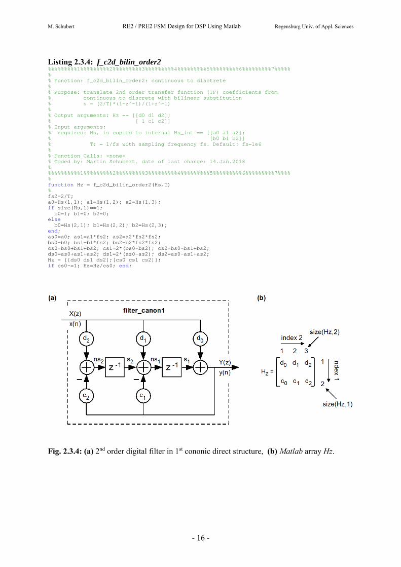
Listing 2.3.4: f_c2d_bilin_order2 %%%%%%%%%1%%%%%%%%%2%%%%%%%%%3%%%%%%%%%4%%%%%%%%%5%%%%%%%%%6%%%%%%%%%7%%%%% % % Function: f_c2d_bilin_order2: continuous to disctrete % % Purpose: translate 2nd order transfer function (TF) coefficients from % continuous to discrete with bilinear substitution % s = (2/T)*(1-z^-1)/(1+z^-1) % % Output arguments: Hz == [[d0 d1 d2]; % [ 1 c1 c2]] % Input arguments: % required: Hs, is copied to internal Hs_int == [[a0 a1 a2]; % [b0 b1 b2]] % T: = 1/fs with sampling frequency fs. Default: fs=1e6 % % Function Calls: <none> % Coded by: Martin Schubert, date of last change: 14.Jan.2018 % %%%%%%%%%%1%%%%%%%%%2%%%%%%%%%3%%%%%%%%%4%%%%%%%%%5%%%%%%%%%6%%%%%%%%%7%%%% % function Hz = f_c2d_bilin_order2(Hs,T) % fs2=2/T; a0=Hs(1,1); a1=Hs(1,2); a2=Hs(1,3); if size(Hs,1)==1; b0=1; b1=0; b2=0; else b0=Hs(2,1); b1=Hs(2,2); b2=Hs(2,3); end; as0=a0; as1=a1*fs2; as2=a2*fs2*fs2; bs0=b0; bs1=b1*fs2; bs2=b2*fs2*fs2; cs0=bs0+bs1+bs2; cs1=2*(bs0-bs2); cs2=bs0-bs1+bs2; ds0=as0+as1+as2; ds1=2*(as0-as2); ds2=as0-as1+as2; Hz = [[ds0 ds1 ds2];[cs0 cs1 cs2]]; if cs0~=1; Hz=Hz/cs0; end;

Fig. 2.3.4: (a) 2nd order digital filter in 1st cononic direct structure, (b) Matlab array Hz.


- 17 -

4.2.5 More Exercises

Fig. 2.3.5: Rth order digital filter in 1st cononic direct structure Fig. 2.3.5 shows a general IIR filter in 1st canonical direct structure with order R. Try to realize it and compare it for R=2 with our 2nd order filter. Respect fact, that for any size of Hz we may make many mistakes or have a numerator only, i.e. an FIR filter where all ci=0. This can be detected from size(Hz,1) == 0. Optimization: Such filters are either very long FIR filters (i.e. all ci=0) or relatively short with large bit-width. Optimization could avoid multiplication with zero ci’s.


- 18 -

5 Time-Discrete Windows, Low-, Band- and High-Passes 5.1 Generate a Blackman-Harris Window

5.1.1 Self-made Blackman-Harris Window

Window functions are of great importance for digital signal processing. In the ideal case they approximate a Gaussian shape with the difference that they come down to zero within a given window on the abscissa. Well known is the Blackman-Harris Window given by BlackmanHarris = a0 - a1*cos(phi) + a2*cos(2*phi) - a3*cos(3*phi) with a0=0.35875, a1=0.48829, a2=0.14128, a3=0.01168. To illustrate this window we write a Matlab function: Blackman-Harris Window, File f_blackmanharris.m

function blackmanharris = f_blackmanharris(cTaps) a0=0.35875; a1=0.48829; a2=0.14128; a3=0.01168; % sum_ai = a0 + a1 + a2 + a3 % should deliver 1 % dif_ai = a0 - a1 + a2 - a3 % should deliver 6e-5 t=0:cTaps-1; phi=2*pi*t/(cTaps-1); blackmanharris = a0 - a1*cos(phi) + a2*cos(2*phi) - a3*cos(3*phi); The sum of all coefficients and therefore the peak of the window function is 1. At the ends of the window the function value is a0-a1+a2-a3=6·10-5. The following testbench plots the window assuming the function. Testbench for Blackman-Harris Window, File tb_blackmanharris.m

% Testbench for Blackman-harris Window Function win11 =f_blackmanharris(11); % 11 points win100=f_blackmanharris(100); % 100 points figure(1); subplot(211); % 2 rows, 1 col, plot into 1st field stem(win11),hold on; plot(win11,'-.'); hold off; subplot(212); % 2 rows, 1 col, plot into 2nd field stem(win100),hold on; plot(win100,'-.'); hold off; The Matlab command » tb_blackmanharris produces the graphics below. Fig. 3.1.1: Blackman-Harris windows with 11 and 100 taps.


- 19 -

5.1.2 Matlab’s Minimum 4-Term Blackman-Harris Window (copied from Matlab)

Comparison of Selfmade with Matlab’s Blackman-Harris Window.

Matlab’s Blackman-Harris has an important difference to the authors window: The author generates a horizontal and Matlab a vertical vector, that can be transposed by the tick: f_blackmanharris(100) = blackmanharris(100)' and vice versa.

Matlab Syntax

w = blackmanharris(L)

Description

w = blackmanharris(L) returns an L-point, minimum , 4-term Blackman-Harris window in the column vector w. The window is minimum in the sense that its maximum side lobes are minimized.

Examples

Create a 32-point Blackman-Harris window and display the result using WVTool: L=32; wvtool(blackmanharris(L))

Fig. 2.4.1.2: Blackman-Harris windows with 32 taps in Matlab’s waveform viewer tool (wvtool).

Algorithm

The equation for computing the coefficients of a minimum 4-term Blackman-Harris window is

where and the window length is .

The coefficients for this window are: a0 = 0.35875; a1 = 0.48829; a2 = 0.14128; a3 = 0.01168

References

Harris, F. J. "On the Use of Windows for Harmonic Analysis with the Discrete Fourier Transform." Proceedings of the IEEE. Vol. 66 (January 1978). pp. 51-84.

See Also

barthannwin, bartlett, bohmanwin, nuttallwin, parzenwin, rectwin, triang, window, wintool, wvtool


- 20 -

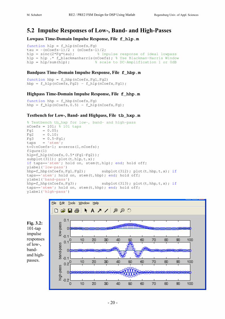
5.2 Impulse Responses of Low-, Band- and High-Passes Lowpass Time-Domain Impulse Response, File f_hlp.m

function hlp = f_hlp(nCoefs,Fg) tau = -(nCoefs-1)/2 : (nCoefs-1)/2; hlp = sinc(2*Fg*tau); % Impulse response of ideal lowpass hlp = hlp .* f_blackmanharris(nCoefs); % Use Blackman-Harris Window hlp = hlp/sum(hlp); % scale to DC-Amplification 1 or 0dB Bandpass Time-Domain Impulse Response, File f_hbp.m

function hbp = f_hbp(nCoefs,Fg1,Fg2) hbp = f_hlp(nCoefs,Fg2) - f_hlp(nCoefs,Fg1); Highpass Time-Domain Impulse Response, File f_hhp.m

function hhp = f_hbp(nCoefs,Fg) hhp = f_hlp(nCoefs,0.5) - f_hlp(nCoefs,Fg); Testbench for Low-, Band- and Highpass, File tb_hxp.m

% Testbench tb_hxp for low-, band- and high-pass nCoefs = 101; % 101 taps Fg1 = 0.05; Fg2 = 0.10; Fg3 = 0.5-Fg1; taps = 'stem'; t=0:nCoefs-1; x=zeros(1,nCoefs); figure(1) hlp=f_hlp(nCoefs,0.5*(Fg1-Fg2)); subplot(311); plot(t,hlp,t,x); if taps=='stem'; hold on, stem(t,hlp); end; hold off; ylabel('low-pass') hbp=f_hbp(nCoefs,Fg1,Fg2); subplot(312); plot(t,hbp,t,x); if taps=='stem'; hold on, stem(t,hbp); end; hold off; ylabel('band-pass') hhp=f_hhp(nCoefs,Fg3); subplot(313); plot(t,hhp,t,x); if taps=='stem'; hold on, stem(t,hhp); end; hold off; ylabel('high-pass') Fig. 3.2: 101-tap impulse responses of low-, band- and high- passes.


- 21 -

6 Computing Frequency Responses of LTI Models 6.1 Time-Continuous Modeling In the time-continuous domain the Fourier transformation

dtetxtxFjX tj )()}({)( (4.1-1)

is useful but has some problems, amongst others with convergence. Such problems are ameliorated by Laplace transformation

dtetxtxLsX st)()}({)( with s= α + j. (4.1-2)

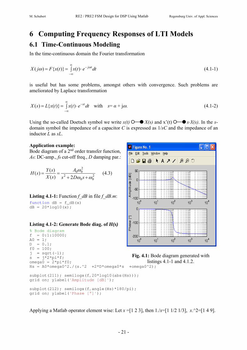
Using the so-called Doetsch symbol we write x(t) X(s) and x’(t) sX(s). In the s-domain symbol the impedance of a capacitor C is expressed as 1/sC and the impedance of an inductor L as sL. Application example: Bode diagram of a 2nd order transfer function, A0: DC-amp., f0 cut-off freq., D damping par.:

200

2

200

2)(

)()(

sDs

A

sX

sYsH (4.3)

Listing 4.1-1: Function f_dB in file f_dB.m: function dB = f_dB(x) dB = 20*log10(x); Listing 4.1-2: Generate Bode diag. of H(s) % Bode diagram f = 0:1:10000; A0 = 1; D = 0.1; f0 = 100; j = sqrt(-1); s = j*2*pi*f; omega0 = 2*pi*f0;

Fig. 4.1: Bode diagram generated with

listings 4.1-1 and 4.1.2. Hs = A0*omega0^2./(s.^2 +2*D*omega0*s +omega0^2); subplot(211); semilogx(f,20*log10(abs(Hs))); grid on; ylabel('Amplitude [dB]'); subplot(212); semilogx(f,angle(Hs)*180/pi); grid on; ylabel('Phase [°]'); Applying a Matlab operator element wise: Let x =[1 2 3], then 1./x=[1 1/2 1/3], x.^2=[1 4 9].


- 22 -

6.2 Time-Discrete Modeling

6.2.1 Fast Discrete Fourier Transformation

Let x[n] be a time-discrete function x[n]=x(tn) with tn=nTs where n=0...N-1 and Ts sampling interval, fs=1/Ts sampling frequency. In this case we have to apply the Discrete Fourier Transformation (DFT) defined by

NknjN

nk enxnxFfX /2

1

0][]}[{][

with sk f

N

kf , k=0...N-1. (4.2.1)

A particular form of the DFT is the numerically very efficient Fast Fourier Transform (FFT) used as function fft in the listing below which should be applied on 2M taps, with integer M. Listing 4.2.1: Matlab code of figure right. Top-down: Lowpass impulse response hlp, linear and logarithmic transfer function fft(hlp), test-input signal x and filtered output signal y. % Bode plot by FFT nCoefs=21; Fg=0.2; % Lowpass impulse response, % here with no window function hlp=f_hlp(nCoefs,Fg); figure(1) subplot(511) stem(hlp); grid on; hold on; plot(zeros(1,nCoefs)); hold off; ylabel('hlp'); axis([1 nCoefs -0.2 0.5]); %------- computation of FFT ---------- F = (0:nCoefs-1)/(nCoefs-1); Hlp = fft(hlp); %------------------------------------- subplot(512) plot(F,abs(Hlp)); grid on; axis([0 1 -0.1 1.2]); ylabel('|Hlp|'); subplot(513) plot(F,f_dB(abs(Hlp))); grid on; axis([0 1 -60 10]); hold off; ylabel('|Hlp| [dB]'); t=0:100; F_low=0.1; F_high=0.4321; x=sin(2*pi*F_low*t)+sin(2*pi*F_high*t);y=conv(x,hlp); subplot(514); plot(t,x); grid on; ylabel('FilterIn'); subplot(515); plot(t,y(1:length(t))); grid on; ylabel('FilterOut');

Fig. 4.2.1: Matlab response to listing 4.2.1: Top - down: Lowpass time-domain impulse response, frequency domain responses line-ar and in dB, input signal, filtered output.


- 23 -

Explanations on the Matlab code used:

Matlab function conv(x,hlp) performs a convolution x*y, which has the length of length(x)+length(y)-1.

Function f_dB was declared in listing 4.1.1.

Matlab function fft(x) performs a fast Fourier transformation delivering complex numbers.

Matlab function abs(fft(x)) delivers the amplitude curve within Bode diagram.

Matlab function angle(fft(x)) will deliver the phase information of the Bode diagram.

The filter is obviously poor but it separates F_low<Fg from F_high>Fg quite well as illustrated in the two lowest subplots.

plot(x,y) plots a line connecting points (xi,yi) of the two vectors x, y of same length.

plot(Ax,Ay,Bx,By,Cx,Cy) plots three lines connecting points (Axi,Ayi), (Bxi,Byi), (Cxi,Cyi).

plot(r) with r being a vector of real numbers uses the indices of r, 1,2,...length(r), as abscissa.

plot(c) with c being a vector of complex numbers plots in the complex plane (Re{c},Im{c}).

Problems:

The DFT is defined for periodic functions only. This problem can be overcome by assuming that the actual data vector is repeated periodically. However, this bears impurities if such a periodic repetition of the data vector disturbs the harmonic behavior of the represented frequencies. It is nearly impossible to avoid this problem, since the recorded frequencies may be unknown before application of the DFT. A possible amelioration of this problem can be obtained by the application of window functions. Furthermore, the DFT requires high computational effort.

The FFT requires that the data vector consists of N=2M samples with M being an integer. If this condition is not fulfilled, the rest of the data vector has to be filled, e.g. with zeros.

Note that N time-domain values deliver N frequency-domain values. Consequently the resolution of the transfer function in Fig. 4.2.1 is quite rough and cannot be improved.


- 24 -

6.2.2 Using the z Transformation

Let h(n) = a0, a1, a2, ... ak be the impulse response of a time-discrete filter and x(n)=x(tn) a sampled waveform, whereat tn=nT with T sampling interval. Then y(n) computes as convolution

k

iik inxaknxanxanxanxanxnhny

0210 )()(...)2()1()()(*)()( .

Convolution in one domain (here time) corresponds to a multiplication in the other domain, here frequency represented by z=esT:

)()()()(...)()()()(0

22

110 zXzHzazXzXzazXzazXzazXazY i

k

ii

kk

and consequently ik

ii zazH

0

)( . (4.2.2)

The only differences between listings 4.2.1 and 4.2.2 is (except the 1st comment line) in the computation of Hlp and the relative frequency F, which has significantly more points for the z transformation. Figures 4.2.1 ad 4.2.2 differ only in the 2nd and 3rd subplot. Here the higher resolution of the z transformation becomes visible. Furthermore a need to fill the hlp vector with zeros to 2M taps as done for the FFT is not given for the z transformation. For recursive filters we have

)(

)()(

1

0

zB

zA

zb

za

zHj

k

ji

ik

ii

In this case compute the polynomials A(z) and B(z) and divide them.


- 25 -

Listing 4.2.2: Matlab code of figure right. Top-down: Lowpass impulse response hlp, linear and logarithmic transfer function Hz=Z{hlp}, test-input signal x and filtered output signal y. % Bode plot by FFT nCoefs=21; Fg=0.2; % Lowpass impulse response, % here with no window function hlp=f_hlp(nCoefs,Fg); figure(2) subplot(511) stem(hlp); grid on; hold on; plot(zeros(1,nCoefs)); hold off; ylabel('hlp'); axis([1 nCoefs -0.2 0.5]); %---computation of z Transformation--- F=0:1e-5:1; j=sqrt(-1); z=exp(j*2*pi*F); Hz = zeros(1,length(F)); for i=1:nCoefs; Hz = Hz + hlp(i)*z.^-i; end; Hlp = Hz; %------------------------------------- subplot(512) f=(0:nCoefs-1)/nCoefs; plot(F,abs(Hlp)); grid on; axis([0 1 -0.1 1.2]); ylabel('|Hlp|'); subplot(513) plot(F,f_dB(abs(Hlp))); grid on; axis([0 1 -60 10]); hold off; ylabel('|Hlp| [dB]'); t=0:100; F_low=0.1; F_high=0.4321; x=sin(2*pi*F_low*t)+sin(2*pi*F_high*t);y=conv(x,hlp); subplot(514); plot(t,x); grid on; ylabel('FilterIn'); subplot(515); plot(t,y(1:length(t))); grid on; ylabel('FilterOut');

Fig. 4.2.2: Matlab response to listing 2.1: Top - down: Lowpass time-domain impulse response, frequency domain responses line-ar and in dB, input signal, filtered output.


- 26 -

7 Matlab’s Linear and Time-Invariant (LTI) Systems >> % Create transfer functions using tf and zpk: >> Htf = tf([3 -3], [1 1.1 0.3], -1) % transfer function >> Hzpk = zpk([1], [-0.5 –0.6], 3, -1) % zero-pole-konstant >> % model type conversion: >> Htf_from_Hzpk = tf(Hzpk), Hzpk_from_Htf = zpk(Htf) Complete the following Matlab-statement such, that we get the Matlab echo printed below. (See next page for solutions.) » Htf_s = ................................................... Transfer function: s + 10 ----------------------------- s^4 + 4 s^3 + 6 s^2 + 4 s + 1 Complete the following Matlab-statement such, that we get the Matlab echo printed below. » Htf_z = ................................................... Transfer function: z + 10 ----------------------------- z^4 + 4 z^3 + 6 z^2 + 4 z + 1 Sampling time: 0.001 Convert the time-continuous LTI system Htf_s into time-discrete Htf2_z using the sampling interval T=0.001. Convert the time-discrete LTI system Htf2_z into time-continuous system Htf2_s. Plot the Bode-Diagrams for Htf2_s and Htf2_z on the same plot sheet. Plot the step and impulse responses of Htf2_s and Htf2_z. Given is the FIR impulse response hlp=f_hlp(nCoefs,Fg). As described in chapter 2. Transform it to the LTI system Hlp_z. with fs=1KHz and plot its Bode diagram.


- 27 -

Solution for LTI - Models in Matlab Complete the following Matlab-statement such, that we get the Matlab echo printed below. » Htf_s = tf([1 10], [1 4 6 4 1]) Transfer function: s + 10 ----------------------------- s^4 + 4 s^3 + 6 s^2 + 4 s + 1 Complete the following Matlab-statement such, that we get the Matlab echo printed below. » Htf_z = tf([1 10], [1 4 6 4 1], 0.001) Transfer function: z + 10 ----------------------------- z^4 + 4 z^3 + 6 z^2 + 4 z + 1 Sampling time: 0.001 Convert the time-continuous LTI system Htf_s into time-discrete Htf2_z using the sampling interval T=0.001. Htf2_z = c2d(Htf_s,0.001); Convert the time-discrete LTI system Htf2_z into time-continuous system Htf2_s. Htf2_s = d2c(Htf2_z) Plot the Bode-Diagrams for Htf2_s and Htf2_z on the same plot sheet. bode(Htf_s,Htf2_z); Plot the step and impulse responses of Htf2_s and Htf2_z. step(Htf2_s,Htf2_z); figure; impulse(Htf2_s,Htf2_z); Given is the FIR impulse response hlp=f_hlp(nCoefs,Fg). As described in chapter 2. Transform it to the LTI system Hlp_z. with fs=1KHz and plot its Bode diagram. Hlp_z=tf(hlp, [1 zeros(1,nCoefs-1)],0.001); bode(Hlp_z);


- 28 -

8 Restricting Data Bit-Width The filters above were computed with double-precision floating-point numbers. In reality we will realize them with fixed-point numbers. So we have to use quantization to optimize the number of fractional bits such, that the hardware effort is minimized without loss of filter quality. Detailed descriptions on this topic are given in [7], [8]. To reduce the number of fractional bits to f we can use one of the following three methods [7] presented below. Using =2-f , floor for truncation and round for rounding we define Truncation: xtrunc = floor(x/) (6.1) Rounding: xround = round(x/) (6.2) Bit-vector easy rounding (bver): xbver = floor(x/+0.5) (6.3) Listing 6.1: Quantization using f_q.m. function xq = f_q(x,delta,mode) if nargin>2; if mode=='trunc'; xq=delta*floor(x/delta); elseif mode=='round'; xq=delta*round(x/delta); else % use mode='bver' as default; xq=delta*floor(x/delta+0.5); end; else % use mode='bver' as default % bit vector easy rounding xq=delta*floor(x/delta+0.5); end; Listing 6.2: Quantizer testbench: tb_q.m % Quantizer testbench delta=1; x=-1.75:0.125:1.75; zlin=zeros(1,length(x)); xtrunc = f_q(x,delta,'trunc'); xround = f_q(x,delta,'round'); xbver = f_q(x,delta); subplot(311);stem(x,xtrunc);grid on; hold on; plot(x,zlin); hold off; axis([x(1),x(end),-2.5,2.5]); ylabel('q_t_r_u_n_c'); subplot(312);stem(x,xround);grid on; hold on; plot(x,zlin); hold off; axis([x(1),x(end),-2.5,2.5]); ylabel('q_r_o_u_n_d'); subplot(313);stem(x,xbver);grid on; hold on; plot(x,zlin); hold off; axis([x(1),x(end),-2.5,2.5]); ylabel('q_b_v_e_r'); ylabel('q_b_v_e_r');

Fig. 6.3: Illustration of the differences

between truncation, rounding and bit-vector easy rounding (bver).


- 29 -

Bit-vector easy rounding [7]: The advantage of bit-vector easy rounding (bver) is its easy realization on bit-level. The only difference to mathematically correct rounding is that the negative number –n.5 (n=0,1,2,3... ) rounds to –n instead of –(n+1). Matlab function parameters and defaults: Note that function f_q has three input arguments in listing 6.1, with mode as 3rd input parameter. As it is not necessary to pass all input argument to a function the Matlab parameter nargin is the number of parameters supplied in the actual function call. The statement "if nargin >2; ... else ..." installs the default value for the mode parameter as 3rd argument of f_q. The testbench in listing 6.2. takes advantage of this option when computing xbver with mode='bver' as default value.


- 30 -

9 Delta-Sigma Modulator 9.1 Principle of First Order ΔΣ Modulator This subsection is for students with advanced knowledge in digital signal processing (DSP). For the Matlab models below there is no need to understand Figs. 7.1, but it is enough to translate the detailed figures in the following subsections into finite state machines. A ΔΣ modulator (DSM) generates a pseudo-random data-stream of relatively low bitwidth. It is “pseudo” because the random process is controlled such, that the mean value of the data-stream corresponds to the input value. Like for a pulse-width modulated (PWM) signal decoding is done with a lowpass. But while PWM delivers pulses of different width, a DSM with a 1-Bit output delivers a bit-density using bits of identical width. Fig. 7.1 illustrates the basic theoretical structure of a first order ΔΣ modulator and Fig. 7.2(a) and (b) make the structure more precise. These figures are addressed to students with sufficient DSP background. For this Matlab exercise it is enough to translate Fig. 7.1(c) into a FSM.

ADC

clk

DAC

Ydigital,int digitallowpass

Ydigital

(b)

(a)

X

eq

b

Y

clk(c)

Yanaloganalog

lowpass

quantizer

DAC

Ydigital

b

lowpass Ydigital

mod.

Xdigital

Xanalog

Fig. 7.1: First order ΔΣ-modulator: (a) Principle.(b) applications for A/D and (c) for D/A conversion


- 31 -

9.2 Finite State Machine (FSM) of a First Order ΔΣ Modulator

Xdigital

(a)

Yanaloganalog

lowpass

quantizer

DAC

(b)

z-1Xdigital Yanalog

analoglowpassDAC

digital integrator

(c)

Xdigital

nYdigital

Ydigital

Ydigital

d q

clk r

sns

quantizer

b

xmax

xmin

b

Fig. 7.2: First order ΔΣ modulator for D/A conversion: (a) Principle.(b) integrator resolved and (c) digital circuit to be realized with b=Xmax-Xmin. Identify in Fig. 7.2(c)… (see → next page for solutions) Stimuli: ................................................ NextState: ................................................ State: ................................................ NextState Logic: ................................................ Output Logic: ................................................ Output: ................................................ Which signals MUST be initialized? .....................................


- 32 -

Solution: Stimuli: Xdigital NextState: Input to flipflops: ns State: Output of all flipflops: s NextState Logic: all logic exept state: adder, quantizer, feedback Output Logic: quantizer (Very formally we could use two quantizers, one for the feedback loop and one as output logic.) Output: Ydigital Which signals MUST be initialized? stimulus Xdigital and state s


- 33 -

9.3 Matlab Model of a First Order ΔΣ Modulator Listing 7.3-1: Matlab Model f_dsm1

function y = f_dsm1(x) % initialize (reset) memory s=0; % modulator feedback loop for i=1:length(x), % after restting state s proceed with combinational logic if s<0; y(i)=-1; else y(i)=1; end; % compute NextState ns = x(i) - y(i) + s; % change memory: state s s = ns; end; Listing 7.3-2: Matlab Testbench f_dsm2

F=0.01; t=0:200; x=sin(2*pi*F*t); % Graphics figure(2); subplot(311) % 3 rows, 1 col, plot into 1st stem(t,x); hold on, plot(t,x,'-.'); hold off % apply delta-sigma modulator y = f_dsm1(x); subplot(312); stem(t,y); % apply lowpass after delta-sigma modulator Fg=0.015; nCoefs = 41; hlp = f_hlp(nCoefs,Fg); z = conv(hlp,y); % apply filter using the convolution function % Graphics subplot(313); stem(z); hold on, plot(z,'-.'); hold off The Matlab command » f_dsm_tb produces the graphics below showing input x in subplot 1, the ΔΣ pseudo-random data-stream y in subplot 2 and the lowpass filtered data-stream z in subplot 3. Note that the number of taps of z is the sum of the taps of x plus y minus 1.


- 34 -

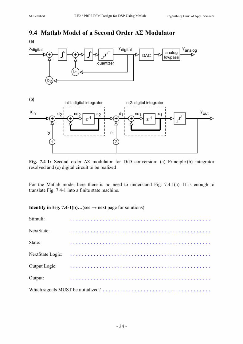
9.4 Matlab Model of a Second Order ΔΣ Modulator

Xdigital

(a)

Yanaloganalog

lowpass

quantizer

DAC

(b)

z-1

Xin

int1: digital integrator

Yout

Ydigital

z-1

int2: digital integrator

2

s2 s1ns2 ns1d2 d1

1

r2 r1

b1

b2

Fig. 7.4-1: Second order ΔΣ modulator for D/D conversion: (a) Principle.(b) integrator resolved and (c) digital circuit to be realized For the Matlab model here there is no need to understand Fig. 7.4.1(a). It is enough to translate Fig. 7.4-1 into a finite state machine. Identify in Fig. 7.4-1(b)…(see → next page for solutions) Stimuli: ................................................ NextState: ................................................ State: ................................................ NextState Logic: ................................................ Output Logic: ................................................ Output: ................................................ Which signals MUST be initialized? .....................................


- 35 -

Solution: Stimuli: Xin NextState: Input to flipflops: ns2, ns1 State: Output of all flipflops: s NextState Logic: the 4 adders, the 2 multipliers b1, b2, quantizer Output Logic: quantizer (Very formally we could use two quantizers, one for the feedback loop and one as output logic.) Output: Yout Which signals MUST be initialized? stimulus Xin and state s1,s2

Listing 7.4-1: Matlab Model f_dsm2

% 2nd Order Delta-Sigma Modulator function [y,s1log,s2log] = f_dsm2(x) % set cofficients b2=1; b1=2; s1log=zeros(1,length(x)); s2log=zeros(1,length(x)); % initialize (reset) memory s1=0; s2=0; % modulator feedback loop y=zeros(1,length(x)); for i=1:length(x); % quantizer: q=4; if q==4; % 4-level quntizer: if s2<-1/2; y(i)=-1.0; elseif s2< 0; y(i)=-1/3; elseif s2< 1/2; y(i)= 1/3; else y(i)= 1.0; end; elseif q==2 % 2-level quntizer: if s2<0; y(i)=-1.0; else y(i)= 1.0; end; else % no quantization y(i) = s2; end; % compute NextState-Vector [ns1,ns2] r2=b2*y(i); d2=x(i)-r2; ns2=d2+s2; r1=b1*y(i); d1=s2-r1; ns1=d1+s1; % apply active clock edge: s1=ns1; s1log(i)=s1; s2=ns2; s2log(i)=s2; end; Listing 7.4-2: Matlab Testbench f_dsm2_tb

F=0.01; t=0:200; x=sin(2*pi*F*t); % Graphics figure(2); CLF; subplot(511) % 5 rows, 1 col, plot into 1st stem(t,x); hold on, plot(t,zeros(1,length(t)),t,x,'-.'); hold off ylabel('x'); % apply delta-sigma modulator [y,s1,s2] = f_dsm2(x); figure(2), subplot(512); stem(t,y); hold on, plot(t,zeros(1,length(t))); hold off ylabel('y');


- 36 -

% apply lowpass after delta-sigma modulator Fg=0.015; nCoefs = 41; hlp = f_hlp(nCoefs,Fg); z = conv(hlp,y); % apply filter using the convolution function % Graphics zt= z(1:length(t)); figure(2), subplot(513); stem(t,zt); hold on, plot(t,zeros(1,length(t)),t,zt,'-.'); hold off; ylabel('lowpass(y)'); % Debugging if 1>0; smax(1)=max(s1); smin(1)=min(s1); smax(2)=max(s2); smin(2)=min(s2); smax,smin, figure(2), subplot(514); stem(t,s1); hold on, plot(t,zeros(1,length(t)),t,s1,'-.'); hold off; ylabel('s1'); figure(2), subplot(515); stem(t,s2); hold on, plot(t,zeros(1,length(t)),t,s2,'-.'); hold off; ylabel('s2'); end;

Fig. 7.4-2: Results obtained with Matlab model. Subplot 1 (top): Input signal x. Subplot 2: output signal y with 4-level quantizer. Subplot 3: Lowpass filtered output signal using Matlab convolution function. Subplot 4: behavior of state s1. Subplot 5 (bottom): behavior of state s2.


- 37 -

10 Canonical Digital Filter Structures There is no need to understand the theoretical background of Figs. 8.1 and 8.2. For the

Matlab models here is enough to translate those figures into a finite state machine.

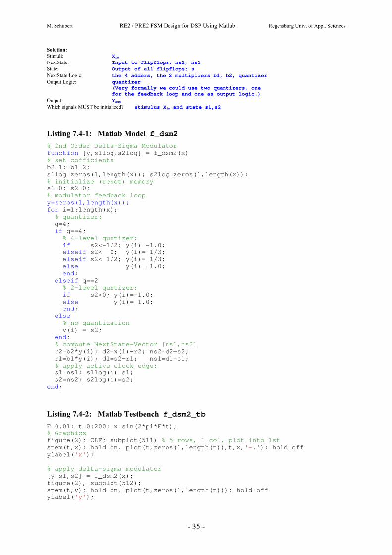
10.1 Digital Filter in the 1st Cononical Direct Structure

z-1 z-1

ac

z-1

yi ,

Y(z)

ac-1 a3 a2 a1

z-1

xi , X(z)

ns1 s1nsc sc s3 s2ns2ns3s4

filter_canon1

Fig. 8.1: Digital Filter in the 1st canonical direct structure Identify in Fig 8.1… (see → next page for solutions) Use the following indexes: i counts time, j counts state values, j=1...c (Matlab: nCoefs:=c) Stimuli: ................................................ State: ................................................ NextState: ................................................ NextState Logic: ................................................ ................................................ Output Logic: ................................................ Output: ................................................ Which signals MUST be initialized? .....................................


- 38 -

Listing 8.1: Matlab Model f_filter_canon1

function y = f_filter_canon1(coefs,x) % % Initializations incl. Reset nCoefs=length(coefs); % get # of Taps of impulse response s = zeros(1,nCoefs); % generate and initialize state ns = zeros(1,nCoefs); % generate nextstate % for i=1:length(x) % % NextState-Logic ns(nCoefs)=coefs(nCoefs)*x(i); for j=nCoefs-1:-1:1; ns(j) = s(j+1) + coefs(j)*x(i); end; % % Output-Logic: compute y(n) y(i) = s(1); % % apply active clock edge s=ns; end; Solutions: Use the following indexes: i counts time, j counts state valuesj, j=1...c (Matlab: nCoefs:=c) Stimuli: x State: Output of all flipflops: sj, j=1…c. NextState: Input to flipflops: nsj (j=1…c) NextState Logic: all MAC (multiply and accumulate) elements: nsc=ac·x, nsj = sj+1 + aj·x, j=c-1...1. Output Logic: none: y = s1 Output: y Which signals MUST be initialized? stimulus x and state sj, j=1…c


- 39 -

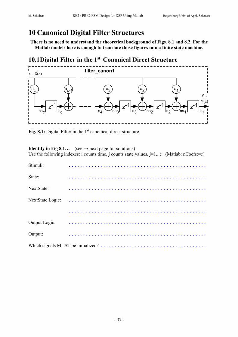
10.2 Digital Filter in the 2nd Cononical Direct Structure

z-1 z-1 z-1

a1

xi ,

X(z)

s1

a2

a3

s2 scns2 ns3 nsc

yi, Y(z)acz-1

s3ns1

filter_canon2

Fig. 8.2: Digital Filter in the 2nd canonical direct structure Identify in Fig 8.2… (→ see previous page for solutions) Use the following indexes: i counts time, j counts state values, j=1...c (Matlab: nCoefs:=c) Stimuli: ................................................ State: ................................................ NextState: ................................................ NextState Logic: ................................................ Output Logic: ................................................ ................................................ Output: ................................................ Which signals MUST be initialized? .....................................


- 40 -

Listing 8.2: Matlab Model f_filter_canon2

function y = f_filter_canon2(coefs,x) % % Initializations incl. Reset nCoefs=length(coefs); s=zeros(1,nCoefs); % initialize state ns=zeros(1,nCoefs); % generate a sufficiently long vector for nextstate % for i=1:length(x) y(i) = 0; % % NextState-Logic ns(1)=x(i); ns(2:nCoefs) = s(1:nCoefs-1); % % Output-Logic: compute y(n) for j=1:nCoefs; y(i) = y(i) + coefs(j)*s(j); end; % % apply active clock edge s=ns; end; Solutions: Use the following indexes: i counts time, j counts state valuesj, j=1...c (Matlab: nCoefs:=c) Stimuli: x State: Output of all flipflops: sj, j=1…c. NextState: Input to flipflops: nsj (j=1…c) NextState Logic: ns1=x, nsj = sj-1 , j=2...c. MUST: bit-accurate! Output Logic: all MAC (multiply and accumulate) elements: a1 s1 + a2 s2 + ... + ac sc Output: y Which signals MUST be initialized? stimulus x and state sj, j=1…c


- 41 -

10.3 Possible Improvements:

10.3.1 Halve the Number of Multipliers

According to the canonic-filter formulae the output value yi of a finite impulse response FIR filter is computed as yi = a1 xi-1 + a2 xi-2 + a3 xi-3 + … + ac-2 xi-(c-2) + ai-1 xi-(c-1) ac xi-c The coefficients for such FIR filters are symmetric, i.e. a1=ac, a2=ac-1, a3=ac-2, ... . Therefore we can save multipliers computing yi = a1 (xi-1+xi-c) + a2 (xi-2+xi-(c-1)) + ... + ac/2 (xi-c/2 + ac+1-c/2) when c is even and yi = a1 (xi-1+xi-c) + a2 (xi-2+xi-(c-1)) + ... + a(c+1)/2 xi-(c+1)/2 when c is odd. 10.3.2 Multiple Use of Multipliers in a Hardware-Realization

When multipliers in your hardware (e.g. FPGA) are much faster than required, one multiplier can be used subsequently to compute several taps. Example: We have a Multiplier that can operate at 40MHz and need an audio filter for a sampling rate of 40KHz. Theoretically, one multiplier can perform 1000 multiplications between two output taps of the filter.


- 42 -

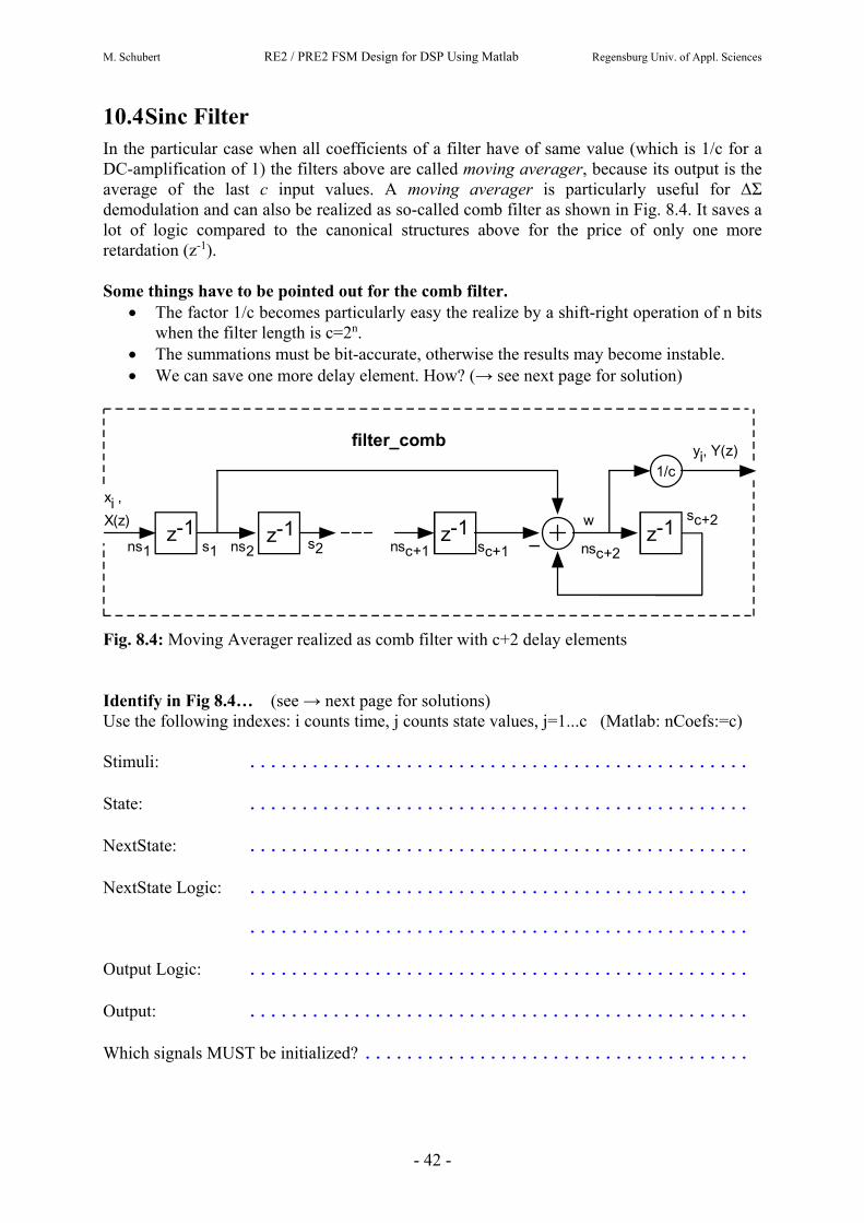
10.4 Sinc Filter In the particular case when all coefficients of a filter have of same value (which is 1/c for a DC-amplification of 1) the filters above are called moving averager, because its output is the average of the last c input values. A moving averager is particularly useful for ΔΣ demodulation and can also be realized as so-called comb filter as shown in Fig. 8.4. It saves a lot of logic compared to the canonical structures above for the price of only one more retardation (z-1). Some things have to be pointed out for the comb filter.

The factor 1/c becomes particularly easy the realize by a shift-right operation of n bits when the filter length is c=2n.

The summations must be bit-accurate, otherwise the results may become instable. We can save one more delay element. How? (→ see next page for solution)

z-1 z-1

xi ,

X(z)

s1 s2 sc+1ns2 nsc+1

yi, Y(z)

z-1ns1

filter_comb

z-1

1/c

sc+2

nsc+2

w

Fig. 8.4: Moving Averager realized as comb filter with c+2 delay elements Identify in Fig 8.4… (see → next page for solutions) Use the following indexes: i counts time, j counts state values, j=1...c (Matlab: nCoefs:=c) Stimuli: ................................................ State: ................................................ NextState: ................................................ NextState Logic: ................................................ ................................................ Output Logic: ................................................ Output: ................................................ Which signals MUST be initialized? .....................................


- 43 -

Solutions to the exercise next page: Stimuli: x State: Output of all flipflops: sj, j=1…c+2. NextState: Input to flipflops: nsj (j=1…c+2) NextState Logic: ns1=x, nsj = sj-1 , j=2...c+1, nsc+2=w=s1-sc+1+sc+2, MUST be bit-accurate! Output Logic: adder, multiplier w·(1/c), =bithshift if c=2n. Output: y Which signals MUST be initialized? stimulus x and state sj, j=1…c+2 How to save one more delay element in the comb filter:

z-1 z-1

xi ,

X(z)

s1 s2

sN+1

ns2 nsN

yi, Y(z)

z-1ns1

filter_comb

z-1sN

nsN+1 wa

Fig. 8.4 modified: Moving Averager realized as comb filter with only c+1 delay elements

NextState Logic: ns1=x, nsj = sj-1 , j=2...c, nsc+1=w-sc, w=s1+sc+1, MUST be bit-accurate! Output Logic: adder u=s1-sc+1, mult. w/c (bithshift if c=2n)


- 44 -

10.5 Testbench for the filter Models Listing 8.4: Testbench f_filter_canon2 for f_filter_canon1 and …2 F=0.01; t=0:200; x=sin(2*pi*F*t); % Graphics figure(4) subplot(411) % 3 rows, 1 col, plot into 1st stem(t,x); hold on, plot(t,x,'-.'); hold off % apply delta-sigma modulator y = f_dsm2(x); subplot(412); stem(t,y); % apply lowpass after delta-sigma modulator Fg=0.015; % cut-off frequency of the lowpass nCoefs = 41; % count of non-zero taps of the lowpass hlp = f_hlp(nCoefs,Fg); z1 = f_filter_canon1(hlp,y); z2 = f_filter_canon2(hlp,y); % Graphics subplot(413); stem(t,z1); hold on, plot(t,z,'-.'); hold off subplot(414); stem(t,z2); hold on, plot(t,z,'-.'); hold off

Fig. 8.5: Filter results using the testbench: Top-down: (a) Input signal, (b) 2-bit output signal of 2nd order ΔΣ-modulator dsm2, (c) Filter 1 applied to (b) and (d) Filter 2 applied to (b)


- 45 -

11 Matlab’s Filter Design & Analysis Tool (fdatool) To get optimized coefficients for a digital filter design use Matlab’s fdatool. Windows: Start -> Programme -> Mathematik -> Matlab R2008a -> Matlab R2008a Within the Matlab Command Window Matlab command window » fdatool Within the fdatool window settings: lowpass, FIR equiripple, minimum order, Density Factor=20 Fs=1000 % sampling frequency Fpass=100 Apass=1 % -3dB passband edge and passband damping Fstop=165 Astop=80dB % -80dB stopband edge and passband damping Desing Filter => Order=39 File -> Export -> as coefficients to Workspace, Numerator=Num -> Export Analysis-> Filter Coefficients Matlab command window » Num % rounded to 5 places after decimal point Matlab command window » Num*1024 % more significant positions visible 0.5724 -2.1857 -5.2453 -9.3015 -12.7120 -12.9667 -7.9518 2.2831 14.3259 21.9483 18.8446 2.6658 -21.7712 -42.4045 -44.0240 -15.3293 44.3000 122.0629 195.1539 239.4135 239.4135 195.1539 122.0629 44.3 -15.3293 -44.0240 -42.4045 -21.7712 2.6658 18.8446 21.9483 14.3259 2.2831 -7.9518 -12.9667 -12.7120 -9.3015 -5.2453 -2.1857 -0.5724 Fig. 9: fdatool window: Lowpass ampli-tude characteris-tic for the 40 filter coefficients listed above.


- 46 -

12 Conclusions Within this tutorial the author demonstrated how to use simple Matlab commands to verify the finite state machine (FSM) design of a counter. Matlab commands are introduced such, that users without knowledge of Matlab can learn the required skills “on the job”. The examples were taken from the field of digital signal processing (DSP) with emphasis on delta-sigma (ΔΣ) modulation and digital filtering using finite impulse response (FIR) filters. An understanding of the theoretical background of these modulators and filters is not necessary, as this tutorial is focused on realizing rather than designing these building blocks.

13 References [1] Open SystemC Initiative (OSCI), available: http://www.systemc.org/news/events/ [2] A. Angermann, M. Beuschel, M. Rau, U. Wohlfarth: „Matlab – Simulink – Stateflow,

Grundlagen, Toolboxen, Beispiele“, Oldenbourg Verlag, ISBN 3-486-57719-0, 4. Auflage (für Matlab Version 7.0.1, Release 14 mit Service Pack 1).

[3] Simulink HDL Coder: Generate HDL code from Simulink models and MATLAB code, available: http://www.mathworks.de/products/slhdlcoder/.

[4] Available http://octave.sourceforge.net/. [5] Available http://de.wikipedia.org/wiki/Scilab [6] M. Schubert, Script “Systemkonzepte”, Regensburg University of Applied Sciences,

available: http://homepages.fh-regensburg.de/~scm39115/ Offered Education Courses and Laboratories SK

[7] M. Schubert, “Using Fixed-Point Numbers”, Electronic Design Automation Course, Regensburg University of Applied Sciences, available: http://homepages.fh-regensburg.de/~scm39115/ Offered Education Courses and Laboratories RED

[8] M. Schubert, “FSM Design for DSP Using VHDL”, Electronic Design Automation Course, Regensburg University of Applied Sciences, available: http://homepages.fh-regensburg.de/~scm39115/ Offered Education Courses and Laboratories RED

[9] S. R. Norsworthy, R. Schreier, G. C. Temes, „Delta-Sigma Data Converters“, IEEE Press, 1996, IEE Order Number PC3954, ISBN 0-7803-1045-4.

[10] J. C. Candy, G. C. Temes, 1st paper in “ Oversampling Delta-Sigma Data Converters, Theory, Design and Simulation”, IEEE Press, IEEE Order #: PC0274-1, ISBN 0-87942-285-8, 1991.

[11] B. Black, R. Ranzenberger, „A/D-Umsetzung – aber richtig“, Elektronik 24, 30. Nov. 1999, pp. 60-66.

[12] www.analog.com/support/standard_linear/practical_design_techniques/section#.pdf, mit # = 3,4,5

[13] C. A. Leme, “Oversampling Interfaces for IC Sensors”, Physical Electronics Laboratory, ETH Zurich, Diss. ETH Nr. 10416.

4 fsm-design 4dsp using matlab - oth regensburg · pdf filethis tutorial is intended to be...

Documents