4. accelerated testing - chapter 4

8/11/2019 4. Accelerated Testing - Chapter 4

http://slidepdf.com/reader/full/4-accelerated-testing-chapter-4 1/30

I

C H A P T E R 4

P A R A M E T E R ES T I M A T I O N

Many methods are available for parameter estimation. I n rel iabil i ty engineering, the most popular

methods are the

f o l l o wi n g :

•

Maximum

likelihood estimation

• Probability plotting

• Hazard plotting

I t is desirable for a parameter estimator to have the f o l l o wi n g properties:

1. L a c k

of

B i a s I f the expected value of the estimator is equal to the true value of the param

eter, it is said to be unbiased.

2. Minimum Variance

—

The smaller the variance of the estimate, the smaller the sample size

required to obtain the level of accuracy desired, and the more efficient the estimator. The

most efficient estimator is the estimator w i t h

minimum

variance.

3. Consistency—

As

the sample size is increased, the value

o f

the estimated parameter

becomes

closer to the true value of the parameter.

4. Sufficiency

—

The estimator uses all information available in the data set.

The method used to estimate parameters depends on the type of data or testing

involved

and the

distribution o f interest. In addition to these parameter estimation methods, this chapter describes

censored data and

presents

methods o f parameter estimation for the exponential, normal, lognor-

mal, and W e i b u l l

distributions.

Methods are presented for complete and censored data.

Maximum

Likelihood

Estimation

Maximum

likelihood is the most widely used method o f generating estimators. I t is based on the

principle of determining the parameter(s) value(s) that maximize(s) the probability of

obtaining

the sample data.

The

likelihood

function for a

given

distribution is a representation of the probability of obtaining

the sample data. Let x\, x

2

,..., x

n

be independent random variables f rom the probability density

function / (x, 0), where G is the single distribution parameter. Then

Z ( x

1

, x

2

, . . . , x „ ; 6 ) =

/(x

1

,e

)/(x

2

,9).../(x

„,e (4.1)

-73-



ACCELERATED TESTING

is the j o i n t distribution of the random variables, or the

likelihood

function. The maximum l i k e l i

hood

estimate,

6, maximizes the likelihood function. This estimate is asymptotically normal.

Often,

the natural logarithm of the likelihood function is maximized to s impl i fy computations.

The

variances

of the

estimates

can be found by inverting the matrix of the negative of the

second

partial derivatives of the

likelihood

function, also known as the local information matrix.

These

estimates are asymptotically normal, and the variances obtained

f rom

the local information matrix

are

used

to calculate confidence intervals.

Probability Plotting

Probability plotting is a graphical method of

parameter

estimation. For the

assumed

distribution,

the cumulative distribution function is transformed to a linear expression, usually by a logarithmic

transformation, and plotted. I f the plotted points fo rm a straight line, the

assumed

distribution is

acceptable, and the slope and the intercept of the plot provide the information needed to estimate

the parameters of the distribution of interest. The median rank is usually used to estimate the

cumulative distribution function, although there are

several

alternatives

such

as the

mean

rank

and the Kaplan-Meier product

l i m i t

estimator.

I f manually constructing a probability plot, distribution-specific probability paper is required.

B y

using probability paper, the failure times and cumulative distribution function estimates

can be plotted directly. W i t h the power of

personal computers

and electronic spreadsheets,

specialized graph paper is no longer needed

because

the necessary transformations can be made

quickly and easily.

Hazard

Plotting

Hazard plotting is a graphical method of parameter estimation. The cumulative

hazard

function

is transformed to a linear expression, usually by a logarithmic transformation, and plotted. The

slope and the intercept of the plot provide the information needed to estimate the parameters of

the distribution of interest.

I f

manually constructing a

hazard

plot, distribution-specific

hazard

paper is required. By using

hazard

paper,

the failure times and cumulative hazard function

estimates

can be plotted directly.

W i t h the power of

personal computers

and electronic

spreadsheets,

specialized graph

paper

is no

longer

needed

because the necessary transformations can be

made

quickly and easily.

Exponential Distribution

The simplest method of

parameter

estimation for the exponential distribution is the method of

maximum likelihood. Maximum likelihood provides an unbiased estimate but no indication oi

goodness of fit. Graphical methods, although more involved, provide a visual goodness-of-fit

test.

Often,

graphical methods

w i l l

be used in conjunction

w i t h

maximum likelihood estimation.

-74-



I

PARAMETER E S T I M A T I O N

Maximum Likelihood Estimation

The exponential

probability

density

function

is

X

/ (* ) = V e , x>0

The maximum likelihood estimation for the parameter 8 is

n

I *

A • 1

=

r

where

x, is the z'th data point (this may be a

failure

or a censoring

point)

«

is the total number of data points (both censored and uncensored)

r is the number of failures

This estimate is unbiased and is the

minimum

variance estimator.

(4.2)

(4.3)

Example 4.1:

Solution:

The cycles to fail for seven springs are:

30,183 14,871 35,031

43,891 31,650 12,310

76,321

Assuming an exponential time-to-fail distribution, estimate the mean time to

fa i l and the mean

failure

rate.

The mean time to fail is

£ 30,183 + 14,871 + 35,031 + 76,321 + 43,891 + 31,650 + 12,310

7

244,257

34,893.9 cycles

The mean

failure

rate is the inverse of the mean time to fail,

1

34,893.9

0.0000287 failures per cycle

Example 4.2:

Assume the data in Example 4.1 represent cycles to fail for seven springs, but

an

additional

10 springs were tested for 80,000 cycles

without

failure.

Estimate

the mean time to fail and the mean failure rate.

- 7 5 -



ACCELERATED

TESTING

Solution:

The mean time to fa i l is

« 244,257 + 10(80,000) ,

6 = - — -

=

149,179.6 cycles

The mean failure rate is

1

149,179.6

0.0000067 failures per cycle

F or a time truncated test, a confidence interval for 0 is

=i

2 '

2 r + 2

<

0 <

i=l

(4.4)

Note that the X degrees of freedom differ for the upper and lower

l imits .

Example 4.3:

Fifteen

items were tested for 1,000 hours. Failures occurred at times oi

120 hours, 190 hours, 560 hours, and 812 hours. Construct a 90% confidence

interval for the mean time to fail and the failure rate.

Solution: This

is a time truncated test. The mean life estimate is

g 120 + 190 + 560 + 812 + 11(1,000) _ 12,682 ,

0

—

—

—

3,170.5

4 4

F or a 90% confidence

interval,

a = 0.1

X

(0.05,10)

=

18.307

5C(0.95,8)

2.733

The 90% confidence

interval

for 0 is

2(12,682)

< <

2(12,682)

18.307 2.733

1,385.5

< 0 < 9,280.6

- 7 6 -



PARAMETER

E S T I M A T I O N

The confidence

interval

for the

failure

rate is the inverse of the confidence

interval for the mean time to fail,

1

s

x

s

1

9,280.6

1,385.5

0.0001077 < X < 0.0007217

F or

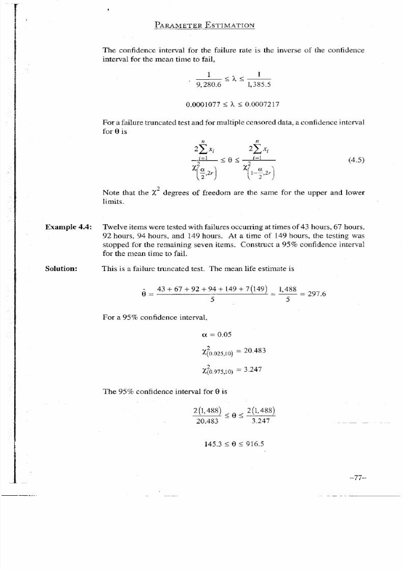
a failure truncated test and for multiple censored data, a confidence interval

for 0 is

2

2 > *

2

E

j

< 0 < - y ^

1

(4.5)

2

Note

that the X degrees of freedom are the

same

for the upper and lower

l imits .

Example

4.4: Twelve items were tested w i t h failures occurring at times of 43 hours, 67 hours,

92 hours, 94 hours, and 149 hours. At a time of 149 hours, the testing was

stopped for the remaining seven items. Construct a 95% confidence interval

for

the mean time to fail.

Solution:

This is a failure truncated test. The mean

l i fe

estimate is

9 - 43 + 67 + 92 + 94 + 149 + 7(149) _ 1,488 _ ^

~T~ " ~ 5 ~

F or a 95% confidence interval,

a = 0.05

XJb.025,10)

=

2 0

-

4 8 3

Z

(0.975,10)

=

3

247

The 95% confidence interval for 0 is

2(1488) ^ 2(1,488)

20.483 3.247 . . _ .

145.3 < 0 < 916.5

- 7 7 -



Example 4.5:

Solution:

ACCELERATED TESTING

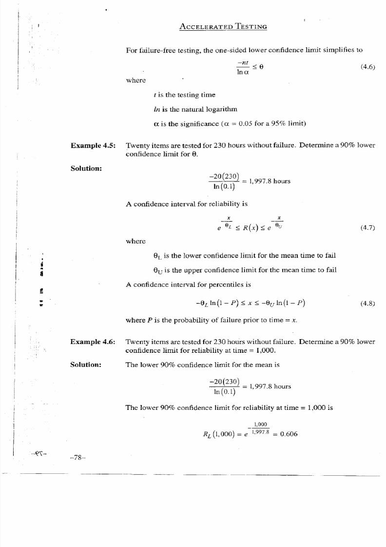
For failure-free testing, the

one-sided

lower

confidence

l i m i t

simplifies to

—nt

In

a

<

9 (4.6)

where

t is the testing time

In is the natural logarithm

a is the significance (a = 0.05 for a 95%

l imi t )

Twenty

items

are

tested

for 230

hours

without failure. Determine a 90% lower

confidence l i m i t

for 0.

-20(230)

In

(0.1)

=

1,997.8

hours

A confidence

interval for reliability is

m

m

e

Q

l

<R(X) < e

where

9

L

is the lower

confidence

l i m i t

for the

mean

time to

fail

Qu is the upper


for the mean time to

fail

A

confidence

interval for

percentiles

is

-Q

L

ln( l -

P) < x < -

ln(l -

P)

where P

is the probability of failure prior to time =

x.

(4.7)

(4.8)

Example 4.6:

Solution:

Twenty

items

are tested for 230

hours

without failure. Determine a 90% lower


for reliability at time = 1,000.

The lower 90%

confidence

l i m i t

for the

mean

is

-20(230)

ln(O. l)

=

1,997.8 hours

The lower 90%

confidence

l i m i t

for reliability at time = 1,000 is

1,000

£ ¿ ( 1 , 0 0 0 )

= e

1

'

9 9 7

'

8

= 0.606

-78-




I

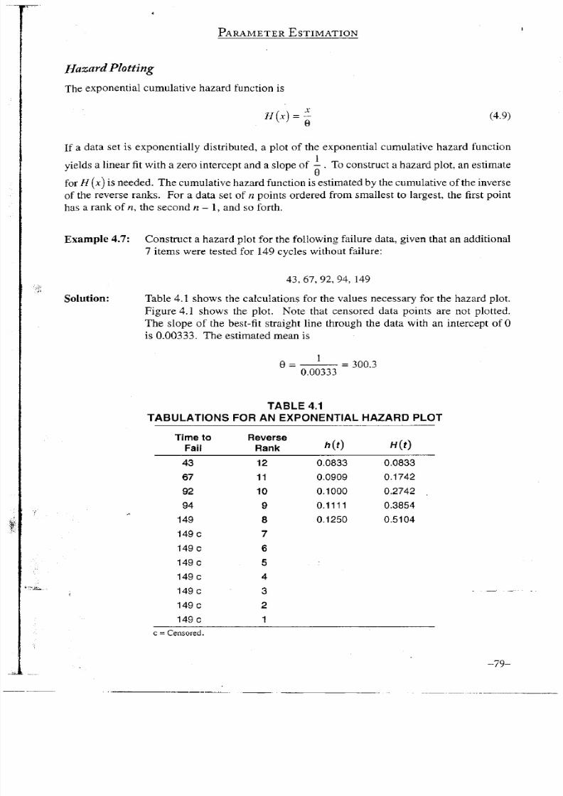
Hazard Plotting

The exponential cumulative hazard function is

» W » f (4-9)

I f

a data set is exponentially distributed, a plot of the exponential cumulative hazard function

yields a linear fi t w i t h a zero intercept and a slope of ^ . To construct a hazard plot, an estimate

fo r H (x)

is needed. The cumulative hazard function is estimated by the cumulative o f the inverse

of

the reverse ranks. For a data set of

n

points ordered

f rom

smallest to largest, the

first

point

has a rank of

n,

the second

n-1,

and so forth .

Example 4.7: Construct a hazard

plot

for the

f o l l o wi n g

failure data, given that an

additional

7

items were tested for 149 cycles

without

failure:

43, 67, 92, 94, 149

Solution: Table 4.1 shows the calculations for the values

necessary

for the hazard

plot.

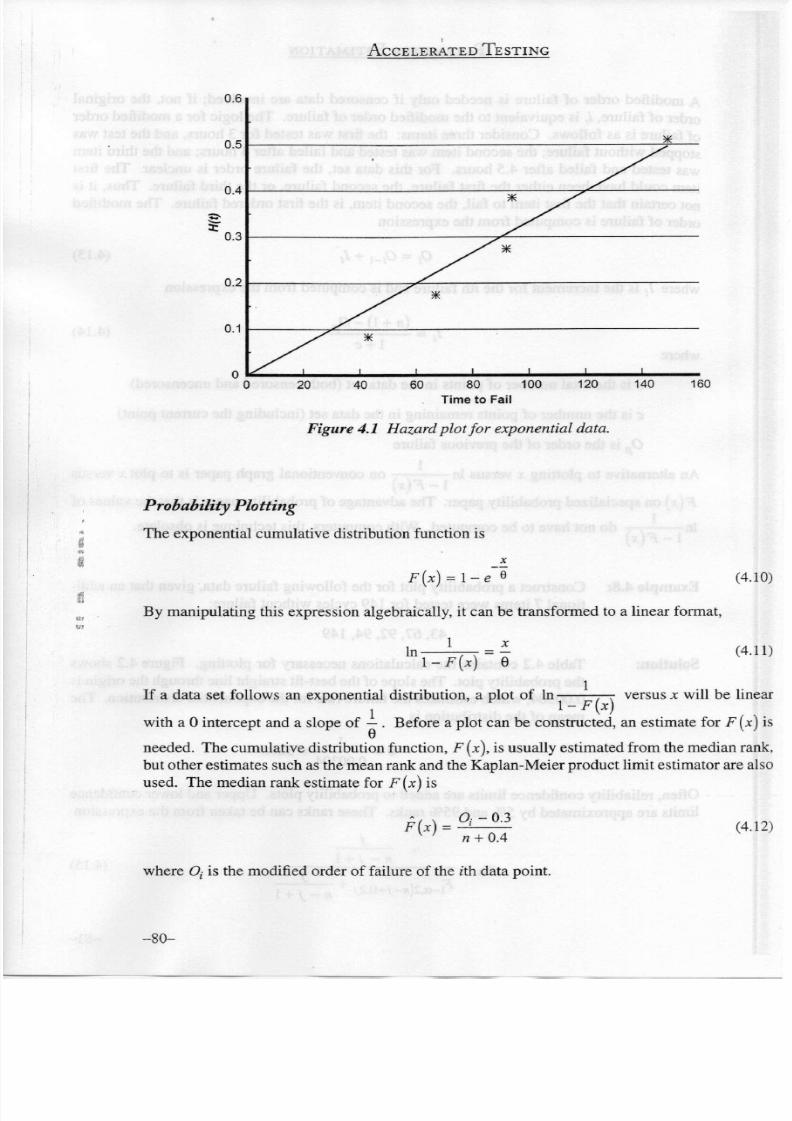
Figure 4.1 shows the plot. Note that censored data points are not

plotted.

The slope of the best-fit straight line through the data w i t h an intercept of 0

is 0.00333. The estimated mean is

9 = = 300.3

0.00333

T A B L E

4.1

T A B U L A T I O N S

F O R

AN E X P O N E N T I A L H A Z A R D

P L O T

Time to

R e v e r s e

h(t)

H(t)

F a i l

R a n k

h(t)

H(t)

43 12

0.0833 0.0833

67

11

0.0909

0.1742

92 10 0.1000 0.2742 ,

94

9

0.1111

0.3854

149

8

0.1250 0.5104

149 c

7

149 c 6

149 c

5

149 c 4

149 c 3

149 c

2

149 c

1

c = Censored.

-79-



ACCELERATED TESTING

0.6

0 20 40 60 80 100 120 140 160

Time to

Fai l

Figure

4.1

Hazard

plot

fo r exponential data.

Probability Plotting

The exponential cumulative

distribution

function is

X

F(x)

= l-e~* (4.10)

B y

manipulating this expression algebraically, it can be transformed to a linear format,

In ^ = ^ (4.H)

l-F(x) 6

I f

a

data

set

follows

an exponential distribution, a plot of In

^—j-r

versus

x

w i l l

be linear

w i t h

a 0 intercept and a slope of — . Before a plot can be constructed, an estimate for

F(x)

is

needed.

The cumulative distribution function, F(x), is usually estimated f rom the median rank,

but other

estimates

such as the mean rank and the Kaplan-Meier product

l i m i t

estimator are

also

used.

The median rank estimate for F

(x)

is

F(

x

)

=

9iZ^l (4.12)

where 0, is the modified order of failure of the ith

data

point.

- 8 0 -



PARAMETER

E S T I M A T I O N

A

modified order of failure is needed only i f censored data are involved; i f not, the

original

order of failure, i, is equivalent to the modified order of failure. The logic for a modified order

of failure is as f o l lo w s . Consider three items: the first was tested for 3 hours, and the test was

stopped

without

failure; the second item was tested and

failed

after 4 hours; and the

th i rd

item

was tested and

failed

after 4.5 hours. For this data set, the

failure

order is unclear. The first

item could have been either the first failure, the second failure, or the t h i r d failure. Thus, it is

not certain that the first item to fa i l , the second item, is the first ordered failure. The modified

order of

failure

is computed f rom the expression

O

i

=O

i

_

l

+ I

i

(4.13)

where /, is the increment for the ith failure and is computed

f rom

the expression

(n

+1) - 0„

L = ^ 1

p

- (4.14)

c

where

n is the total number of points in the data set (both censored and uncensored)

c is the number of points remaining in the data set

(including

the current

point)

O

p

is the order of the previous failure

A n alternative to plotting x versus In ^—T— on conventional graph paper is to plotx versus

l - F ( x )

(x ) on specialized probability

paper.

The advantage of probability paper is that the values of

I n - — j — do not have to be computed. W i t h computers, this technique is obsolete.

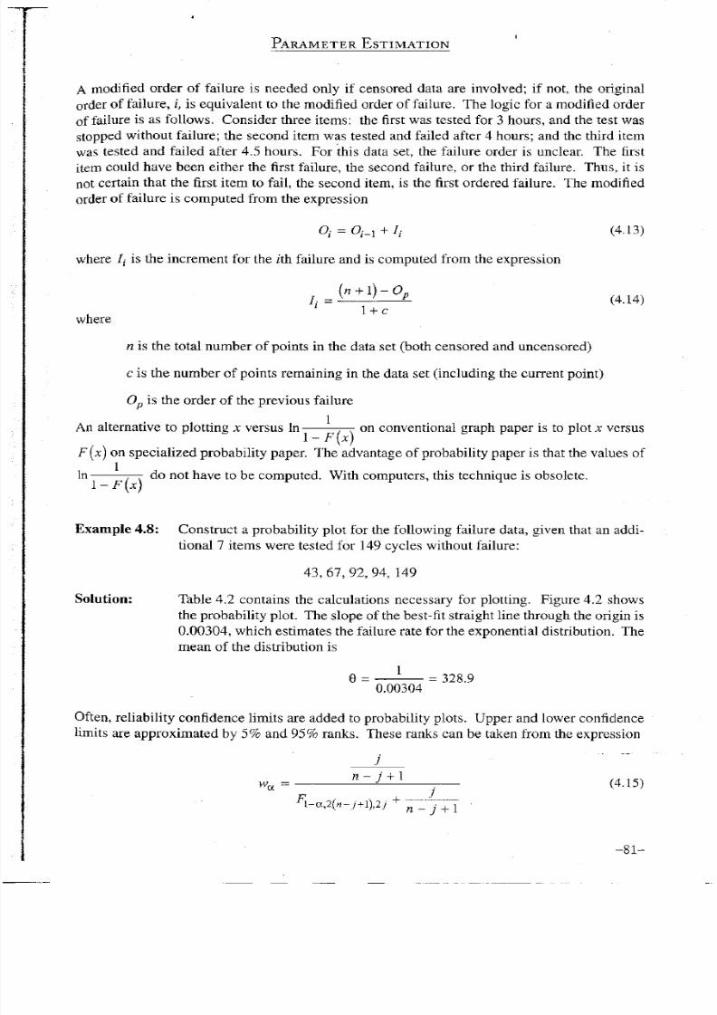
Example

4.8: Construct a

probability

plot for the f o l l o wi n g

failure

data, given that an addi

tional 7 items were tested for 149 cycles without failure:

43, 67, 92, 94, 149

Solution:

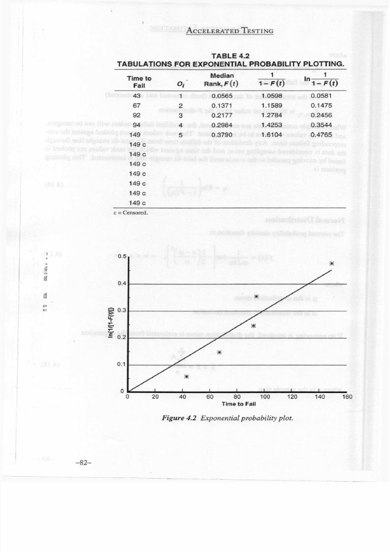
Table 4.2 contains the calculations necessary for plotting. Figure 4.2 shows

the probability plot. The slope of the best-fit straight line through the

or ig in

is

0.00304, which estimates the

failure

rate for the exponential

distribution.

The

mean of the distribution is

0 = = 328.9

0.00304

Often,

re l iab i l i ty

confidence

l im i t s

are added to probability plots. Upper and lower confidence

l imits

are approximated by 5% and 95% ranks. These ranks can be taken

f rom

the expression

w

a

= 1 -.

(4.15)

F

l - a , 2 { n

-j

+ l ) , 2 j

+

n

- j + l '

- 8 1 -



ACCELERATED TESTING

T A B L E 4.2


F O R

E X P O N E N T I A L P R O B A B I L I T Y P L O T T I N G .

T i m e

to

F a i l

o

Median

R a n k , F ( f )

1

1

- F ( t )

In

, c

1

- F ( f )

43

1

0.0565 1.0598

0.0581

67

2

0.1371 1.1589

0.1475

92

3

0.2177 1.2784 0.2456

94

4

0.2984

1.4253

0.3544

149

5

0.3790

1.6104 0.4765

149 c

149 c

149 c

149 c

149 c

149 c

149 c

c

=

Censored.

160

Time

to Fai l

Figure

4.2

Exponential probability

plot.

-82-



PARAMETER

E S T I M A T I O N

where

w

a

is the 100(1 - a )% nonparametric confidence

l imi t

/ is the failure order

n is the total number of data points (both censored and uncensored)

F

aVi

v

is the cri t ical value f rom the F-distribution

When multiple censored data are

encountered,

the modified failure orders w i l l not be integers,

and the rank values w i l l

have

to be interpolated. The rank values are not plotted against the cor

responding failure time. Any deviation of the failure time

f rom

the best-fit straight line through

the data is considered sampling error, and the time against which the rank values are plotted is

found

by moving parallel to the x-axis un t i l the best-fit straight line is intersected. This plotting

position is

X} = Oln

\-F(x

i

)

(4.16)

Normal Distribution

The normal probability density function is

1

GV27T

exp

\(x-\^

—

°° < X < °°

(4.17)

where

p is the distribution mean

G is the distribution

standard

deviation

I f

no censoring is involved, the distribution mean is estimated

f rom

the expression

n

[l

= x =

(4.18)

n

where

n

is the sample

size.

-83-



ACCELERATED TESTING

I f

no censoring is involved, the distribution standard

deviation

is estimated f rom the expression

However, when censored data are

involved,

parameter estimation becomes complicated. Thre

popular

methods for parameter estimation for the

normal distribution

when censored data ai

encountered

are as

fo l lows :

1.

Max imum likelihood estimation

2. Hazard plotting

3. Probability

plotting

The f o l l o wi n g

sections present each of

these

alternatives.

Maximum

Likelihood Estimation

The maximum likelihood equations for the normal distribution are

where


k is the number of censored observations

x

is the sample mean of the failures

s

is the sample standard

deviation

for the failures

z(x) is the standard

normal

deviate

h(xi)

is the hazard function evaluated at the

z'th

point

(4.2(

dL

da

(4.2:

-84-




where

(j)(z(x,-)) is the

standard

normal probability density function evaluated at the zfh point

<E>(z(xj))

is the

standard

normal cumulative distribution function evaluated at the zth

point

Note that i f no

censored

data are involved, these expressions reduce to the

sample mean

and the

sample standard

deviation.

Iterative

techniques

are

necessary

to

these equations.

A

standard

method

based

on Taylor

series

expansions

involves

repeatedly

estimating the

parameters u n t i l

a desired level of

accuracy

is

reached. Estimates

of

p.

and a are given by the

expressions,

respectively,

\ L

t

= i l

M

+ h (4.22)

o~ =a,_i + k

where

h

is a correction factor for the distribution

mean

k

is a correction factor for the distribution

standard

deviation

For

each

iteration, the correction factors are estimated

f rom

the

expressions

dL

u*

2L

h—-

+ k-

d

2

L

dp

2

d\ido d\i

(4.23)

(4.24)

d

2

L , d

2

L dL

h

^ ^

+ k

—o =

dpdo

da oo

(4.25)

where

3p

2

(4.26)

d

2

L

d\id<5

2 ( x - p )

a

i=l

(4.27)

da

2

3{s

2

+ (x -

u)

2

[

k

r

A \ ^ J _

1 +

y Q

i=i

(4.28)

-85-



ACCELERATED TESTING

and

h

(x

i

) [ h

(xj)-z(x

i

)

B

i

=h(x

i

)

+

z(x

i

)A

i

Q ^

z(x

i

)[h(x

i

)

+

(4.29)

(4.30)

(4.31)

The estimated parameters are asymptotically normal. The variances of the estimates can be

found by inverting the local information matrix,

=

d

2

L

d

2

L

d u

2

dpda

d

2

L d

2

L

d[ida

da

2

Afte r

inversion, the variances are

F~

l

=

var(p) cov(p,6~)

cov(p,a) var(o)

Approximate (l - a) 100% confidence intervals for the estimated parameters are

(4.32)

(4.33)

(4.34)

a

exp

< o

<aexp

J

(4.35)

where

K

a

is the inverse of the

standard

normal probability density function.

2

These confidence intervals are approximate but

approach

exactness as the sample size

increases.

Confidence intervals for re l iab i l i ty can be found using the

expressions

var

var(p) +z

2

var(o) + 2zcov(|i,a)

a

2

(4.36)

-86-



ACCELERATED TESTING

Time to Fai l

150c

183 c

235

. 157 c 209

235

167 c '

216c 248 c

179

217 c

257

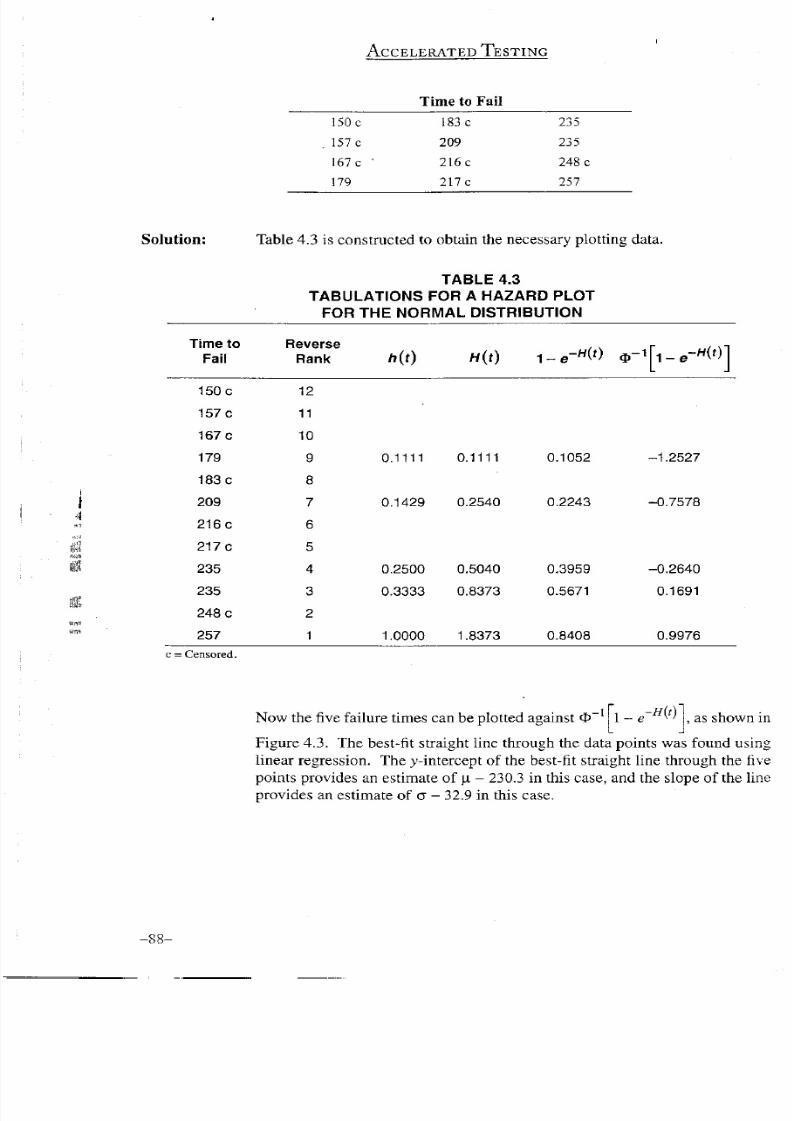
Solution:

Table 4.3 is constructed to obtain the necessary plotting data.

T A B L E 4.3

T A B U L A T I O N S F O R

A

H A Z A R D P L O T

F O R

T HE

N O R M A L

D I S T R I B U T I O N

4

T i m e

to

F a i l

R e v e r s e

R a n k

h ( t )

( 0

1

- e

-

w

W

- l [ i - e - « ) ]

150 c 12

157 c 11

167 c

10

179

9 0.1111

0.1111

0.1052 -1.2527

183 c

8

209

7

0.1429 0.2540 0.2243 -0.7578

216 c

6

217 c 5

235 4

0.2500

0.5040

0.3959

-0.2640

235 3

0.3333

0.8373 0.5671 0.1691

248 c

2

257

1

1.0000

1.8373 0.8408 0.9976

c = Censored.

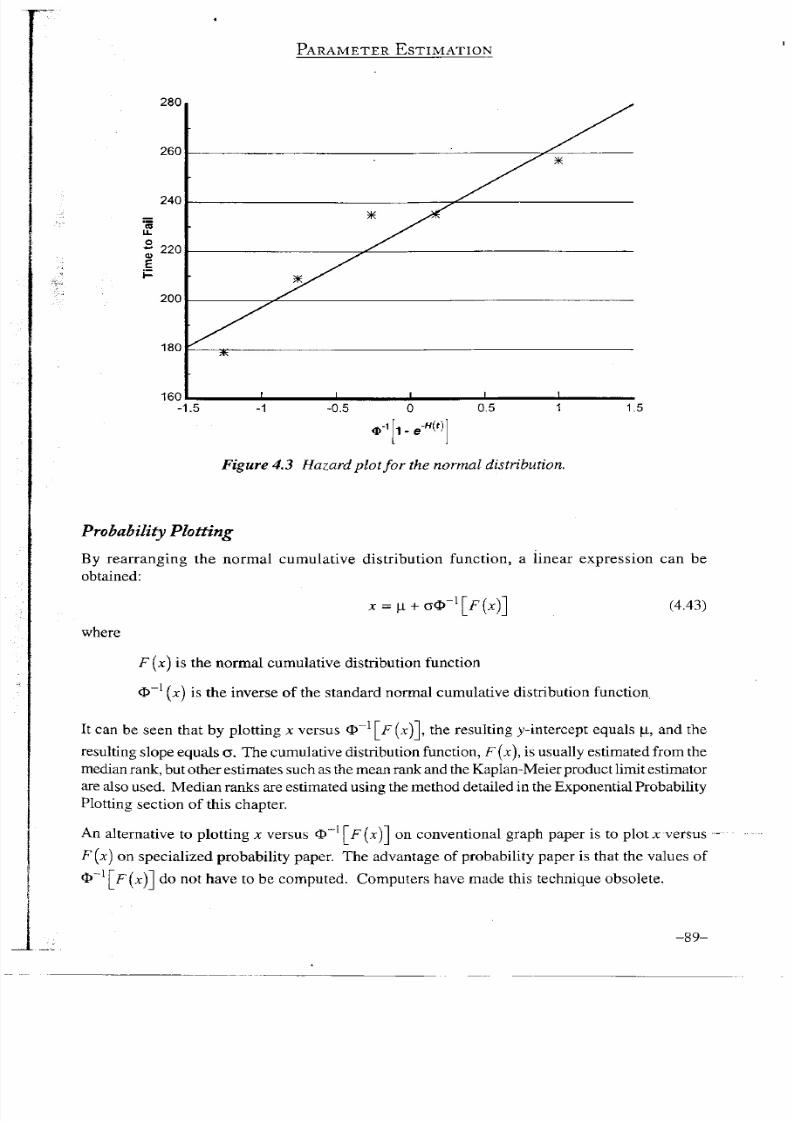
Now the five failure times can be plotted against O

Figure 4.3. The best-fit straight line through the data points was found using

linear regression. The y-intercept of the best-fit straight line through the

five

points

provides an estimate of p - 230.3 in this

case,

and the slope of the line

provides an estimate of o - 32.9 in this case.

-H(t )

as shown in

-88-



PARAMETER

ESTIMATION

280

260

240

u .

o

~ 220

•

E

200

180

160

-1.5 -0.5 0.5 1.5

O

1

1 - e

-H(t)

Figure 4.3 Hazard plot fo r the normal distribution.

Probability

Plotting

By

rearranging the normal cumulative distribution function, a linear expression can be

obtained:

where

x = VL + < r t>~

1

[F(x)] (4.43)

[x] is the normal cumulative distribution function

O

- 1

(x)

is the inverse of the standard normal cumulative

distribution

function

I t

can be seen that by

plotting x versus

O

- 1

[ f (X ) J ,

the resulting y-intercept

equals

p, and the

resulting slope

equals

o. The cumulative distribution function, F (x), is usually estimated

from

the

median rank, but other

estimates

such as the mean rank and the

Kaplan-Meier

product

l imi t

estimator

are

also used.

Median ranks are estimated using the method detailed

i n

the Exponential Probability

Plotting

section of this

chapter.

A n

alternative to plotting x

versus

O

- 1

[ -F ] on conventional graph

paper

is to plot x

versus

(x )

on specialized

probability paper.

The

advantage

of

probability paper

is that the values of

> ~

L

\_F(X)~\

do not

have

to be computed. Computers

have made

this technique obsolete.

- 8 9 -



ACCELERATED TESTING

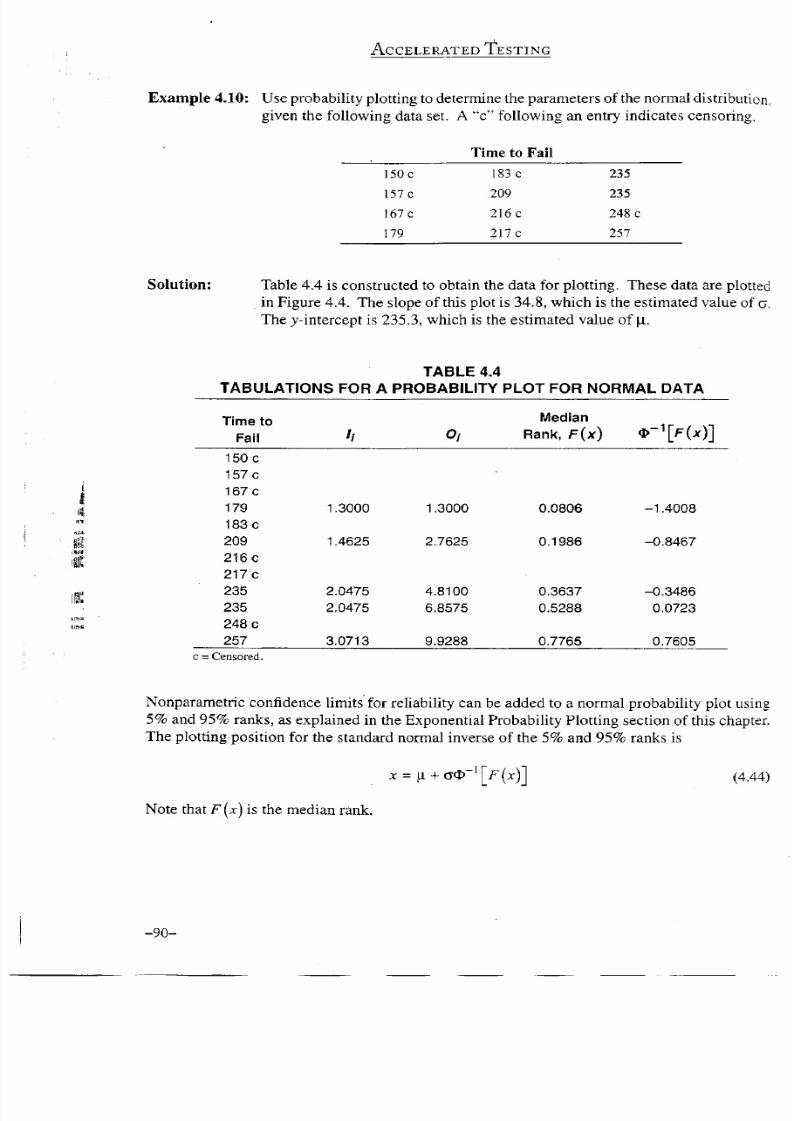
Example 4.10: Use

probability plotting

to determine the parameters of the normal

distribution.

given the

f o l l o w i n g

data set. A "c"

f o l l o w i n g

an entry indicates censoring.

Time to Fa i l

150 c 183 c 235

157 c

209 235

167 c

216c 248 c

179

217 c 257

Solution:

Table 4.4 is constructed to obtain the data for

plotting. These

data are plotted

in Figure 4.4. The slope of this

plot

is 34.8,

which

is the estimated value of o.

The y-intercept is 235.3,

which

is the estimated value of p.

T A B L E

4.4

T A B U L A T I O N S F O R

A

P R O B A B I L I T Y

P L O T

F O R NORM L

D A T A

Time

to

Median

0

1

[ F ( * ) ]

F a i l

/

o,

R a n k , F(x)

0

1

[ F ( * ) ]

150 c

157 c

167 c

179

1.3000 1.3000

0.0806 -1.4008

183 c

209

1.4625

2.7625 0.1986 -0.8467

216c

217c

235

2.0475 4.8100 0.3637

-0.3486

235

2.0475

6.8575 0.5288

0.0723

248 c

257

3.0713

9.9288 0.7765

0.7605

c = Censored.

Nonparametric confidence

l imi ts

for

rel iabil i ty

can be added to a normal

probability plot

using

5% and 95% ranks, as explained in the Exponential Probability

Plotting

section of this chapter.

The plotting position for the standard normal inverse of the 5% and 95% ranks is

x =

p +

a O

- 1

[ F ( x ) ]

(4.44)

Note

that

F ( x)

is the median rank.

-90-



PARAMETER

E S T I M A T I O N

280

-2 -1.5 -1 -0.5 0 0.5 1

0-

1

[F(x)]

Figure

4.4 Normal probability plot.

Lognormal Distribution

The lognormal probability density function is

/W -

1

ÖXJ2K

exp

l f l n x - p ^

2

, x >

0

(4.45)

where

p is the location

parameter

a is the shape parameter

I f x is a lognormally distributed random variable, then y = In (x) is a normally distributed random

variable. The location

parameter

is equal to the

mean

of the logarithm of the

data

points, and

the

shape

parameter is equal to the standard deviation of the logarithm of the data points. Thus,

the lognormal distribution does not have to be dealt w i t h as a

separate

distribution. By taking

the logarithm of the data points, the techniques developed for the normal distribution discussed

in

the previous section can be

used

to estimate the

parameters

of the lognormal distribution^

- 9 1 -



ACCELERATED TESTING

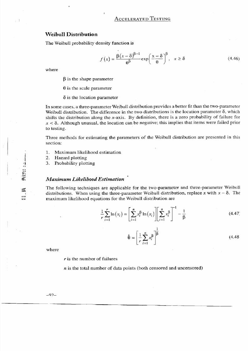
Weibull Distribution

The Weibull probability density function is

f(x)

= ^

X

^

exp ^ —^ ,

x >

8 (4.46)

0P

v

where

P is the

shape parameter

9 is the

scale parameter

8 is the location parameter

I n

some

cases,

a three-parameter

W e i b u l l

distribution provides a

better

fit than the

two-parameter

W e i b u l l

distribution. The difference in the two distributions is the location parameter 5, which

shifts the distribution along the x-axis. By definition,

there

is a

zero

probability of failure for

x < 5. Although

unusual,

the location can be

negative;

this implies

that

items

were

failed prior

to testing.

Three

methods for estimating the parameters of the Weibull distribution are presented in this

section:

1.

Maximum likelihood estimation

2. Hazard plotting

3. Probability plotting

Maximum Likelihood

Estimation

The following

techniques

are applicable for the

two-parameter

and

three-parameter

Weibull

distributions. When using the

three-parameter

Weibull distribution,

replace

x w i t h x - 8. The

maximum likelihood equations for the Weibull distribution are

¡•=1

Z* F

m

(*i)

l

i=l

1

p

(4.47;

9 =

1

i=l

(4.48

where

r

is the

number

of failures

n

is the total

number

of

data

points (both

censored

and

uncensored)



I

ACCELERATED TESTING

^ c W

v a r

(

e

)

< e < eexp

(4.55)

exp

where K

a

is the inverse of the standard normal probability density function.

These confidence intervals are approximate but approach exactness as the sample size increases.

Confidence intervals for

re l iab i l i ty

can be found using the expressions

exp

-exp

u + K

a

Jvar

(w j

V

f

_

< R(x)< exp

-exp

(4.56)

u = p[l n(x)- ln(0)]

(4.57)

var

var

e)

V ^ J

2ucov(p\9)

Confidence intervals for percentiles can be found using the expressions

e

yL

< x < e

yu

I

x = e[ - ln( l - /7) ]p

l n f - l n f l - / ? ) ] , - r

y

L

=

ln,6 +

1

p ^

J

- Kjvar(y)

l n f - l n f o - p ) I — ~ r

yy = ln6 +

L

p ^

J

+ K

ay

lvar{y)

var

W-

var

6̂

(0) { l n [ - l n ( l - p)]}

2

var(P)

2Jln[-ln (l -

/

>)]}cov e,P)

(4.58)

(4.59)

(4.60)

(4.61)

(4.62)

(4.63)

-94-




Hazard Plotting

The

W e i b u l l

cumulative hazard

function

is

H (x )

=-ln[l

- F(x)]

(4.64)

Replacing F

(x )

and rearranging gives a linear expression

l n f f ( x )

=

( j inx-plnO

(4.65)

By plotting

\n H(x ) versus Inx, the resulting slope (censored points are not plotted) provides

an estimate of p. The y-intercept of this

plot

is an estimate of p i n

B .

Thus, 0 is estimated f rom

the expression

P.

6

—

exp

(4.66)

where y

0

1 S

the y-intercept of the hazard plot.

The hazard function h (x) is estimated f rom the inverse of the reverse rank of the ordered failures;

the cumulative hazard

function, H

(x), is the cumulative of the values of

h[x).

An alternative to

plotting In

H

(x ) versus In

x is to

directly plot

H

(x ) versus

x on specialized

W e i b u ll

hazard

paper.

The

advantage

of hazard

paper

is that

logarithmic

transformations do not have to be computed.

Computers have made this technique obsolete.

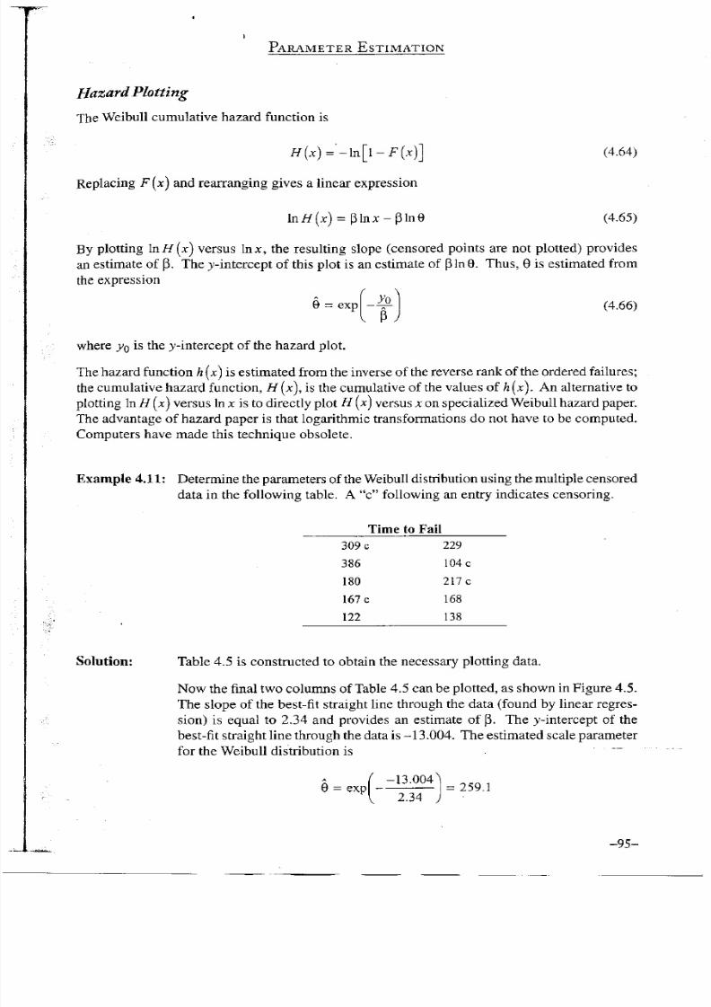
Example 4.11

: Determine the

parameters o f

the

Weibul l

distribution using the multiple censored

data in the f o l l o w i n g table. A "c" f o l l o wi n g an entry indicates censoring.

Time to Fa i l

309 c

229

386

104 c

180

217 c

167 c

168

122 138

Solution:

Table 4.5 is constructed to obtain the necessary

plotting

data.

N ow

the

f inal

two columns

o f

Table 4.5 can be

plotted,

as shown in Figure 4.5.

The slope of the best-fit straight

line

through the

data

(found by linear regres

sion)

is equal to 2.34 and provides an estimate of p. The y-intercept of the

best-fit straight line through the data is -13.004. The estimated

scale

parameter

fo r

the

W e i b u l l distribution

is

exp

-13.004

2.34

= 259.1

- 9 5 -



ACCELERATED TESTING

T A B L E

4.5

T A B U L A T I O N S FOR

A

HAZARD

P L O T

FOR TH E

W E I B U L L

DIST RIBU TION

Time

to

F a i l

R e v e r s e

R a n k

h(t)

f f ( f )

InW(f)

Inf

104 c

10

122

9

0.1111

0.1111

-2.1972 4.8040

138

8 0.1250

0.2361

-1.4435 4.9273

167 c

7

168

6

0.1667

0.4028

-0.9094

5.1240

180

5 0.2000

0.6028

-0.5062 5.1930

217 c

4

229

3

0.3333

0.9361

-0.0660 5.4337

309 c

2

386

1

1.0000

1.9361

0.6607

5.9558

c = Censored.

Figure 4.5 Weibull distribution hazard plot.

-96-




Probability

Plotting

B y taking the

logarithm

of the W e ib u ll cumulative

distribution function

twice and rearranging,

In In

1

l - F ( x )

= plnx-(3ln6

(4.67)

B y

plotting In In versus lnx and f i t t ing a straight line to the points, the parameters

l-F(x)

of the

We ib u l l

distribution can be estimated. The slope of the plot provides an estimate of p,

and the y-intercept can be used to estimate 0,

0 = exp

f

y o

P

(4.68)

The

cumulative distribution function,

F ( x ) , is usually estimated f rom the median rank, but other

estimates such as the mean rank and the Kaplan-Meier product l i m i t estimator are also used.

Median ranks are estimated using techniques shown in the Exponential Probability Plotting sec

t ion of this chapter. Specialized

probability

paper is available for

probability plotting.

Using

probability

paper eliminates the need to transform the data

prior

to

plotting.

Example

4.12: Determine the parameters of the We ib u l l distribution using probability plotting

fo r

the data given in the hazard

plotting

example, Example

4

.11.

Solution:

Table 4.6 is constructed to obtain the necessary plotting data.

T A B L E 4.6


FO R A P R O B A B I L I T Y P L O T

F O R T HE W E I B U L L D I S T R I B U T I O N

Time to

F a i l

/

O;

Median

R a n k ,

F(x)

In

<

1 \

Inf

104 c

122

1.1000 1.1000

0.0769

-2.5252

4.8040

138 1.1000

2.2000

0.1827 -1.6008

4.9273

167 c

168 1.2571 3.4571 0.3036

-1.0167

5.1240

180 1.2571

4.7143

0.4245

-0.5934

5.1930

217c

229

1.5714 6.2857 0.5755

-0.1544 5.4337

309 c

386 2.3571 8.6429 0.8022 0.4827

5.9558

-97-



I

ACCELERATED TESTING

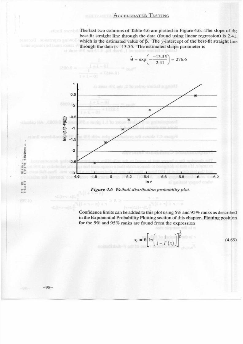
The last two columns of Table 4.6 are plotted in Figure 4.6. The slope of the

best-fit straight line through the data (found using linear regression) is 2.41,

which is the estimated value of

(3.

The y-intercept of the best-fit straight line

through

the

data

is -13.55. The estimated shape

parameter

is

0 = exp

-13.55

2.41

276.6

Confidence

l imits

can be added to this plot using 5% and 95% ranks as described

in

the Exponential Probability

Plotting

section of this

chapter. Plotting

position

for the 5% and 95% ranks are found f rom the expression

In

l - F ( x )

(4.69)

-98-



PARAMETER

E S T I M A T I O N

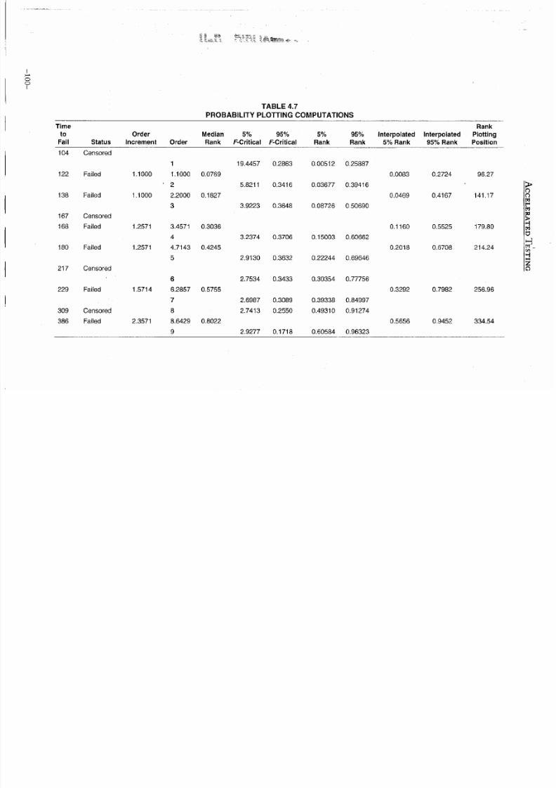
Example 4.13: Repeat Example 4.12, and add 5% and 95% confidence l imits .

Solution:

The 5% and 95% ranks are computed using the f o l l o wi n g expression.

Because

the failure order is not an integer, the 5% and 95% ranks must be interpolated.

Using a failure order of 1, f rom Eq. 4.15 the 5% rank is

1

+

1

1

w

0 0 5

=

1 0

~

1 + 1

, = 0.0051

19.4457 +

1 0 - 1

+ 1

Using

a

failure

order of 2, the 5% rank is

2

w

0 0 5

=

1 0

~

2 + 1

•

- 0.0368

5.8211 +

10- 2 + 1

Interpolating

to a failure order of 1.1 gives a 5% rank of 0.0083. A l l calcula

tions

are shown in Table 4.7.

Figure

4.7 shows the probability

plot w i t h

5% and 95% confidence l imits .

Nonparametric Confidence Intervals

The duration for a bogey test is equal to the re l iab i l i ty requirements being demonstrated. For

example, i f a test i s designed to demonstrate that a component has specific rel iabil i ty at 100 hours,

and the test duration is 100 hours, then the test is designated as a bogey test. Pass-fail tests also

are considered bogey

tests.

A 100(l - a )% nonparametric confidence

interval

for

rel iabil i ty

when bogey testing is

( « - r

+ l )F

- , 2 { n - r + l ) , 2 r

r < R < ; ^ (4.70)

n- r + (r + l)F

a

r + (n-r + l)F

a

| , 2 (r+ l ) ,2 (»-r)

v

'

| , 2 («-r+ l ) ,2r

where

n

is the sample size


F

a > v v

is the

c r i t ica l

value of the

F-distribution

- 9 9 -



o

o

I

T i me

to

Fai l

122

138

167

168

180

217

229

309

386

T A B L E

4.7

P R O B A B I L I T Y

PL O T T I N G C O M P U T A T I O N S

S ta tu s

Order

Median

Increment Order Rank

5

95% 5% 95%

F-Cr i t i ca l F-Cr i t i ca l Rank Rank

Rank

Interpolated

Interpolated Plotting

5 Rank

9 5

Rank P o s i t i o n

104 Censored

Failed

Failed

Censored

Failed

Failed

Censored

Failed

Censored

Failed

1

1.1000 1.1000 0.0769

" 2

1.1000 2.2000 0.1827

3

1.2571 3.4571 0.3036

4

1.2571 4.7143 0.4245

6

1.5714 6.2857 0.5755

7

8

2.3571 8.6429 0.8022

9

19.4457 0.2863 0.00512 0.25887

5.8211 0.3416 0.03677 0.39416

3.9223 0.3648 0.08726 0.50690

3.2374 0.3706 0.15003 0.60662

2.9130 0.3632 0.22244 0.69646

2.7534 0.3433 0.30354 0.77756

2.6987 0.3089 0.39338 0.84997

2.7413 0.2550 0.49310 0.91274

0.0083

0.0469

0.1160

0.2018

0.3292

0.5656

0.2724

0.4167

0.5525

0.6708

0.7982

0.9452

96.27

141.17

179.80

214.24

256.96

334.54

o

w

M

a

M

_

en

H

—

Z

o

2.9277 0.1718 0.60584 0.96323




i

i

4.50 4.70 4.90 5.10 5.30 5.50 5.70 5.90

Inffime)

Figure 4.7 Weibull probability plot with confidence limits.

Example 4.14:

Twenty items are tested,

w i t h

3 items fai l ing and 17 items passing. What is

the 90% confidence interval (two-sided) for

reliability?

Solution:

The

total

sample size,

n,

is 20; the number of failures,

r,

is 3. To compute the

confidence l imi ts , two

c r i t ica l

values

f rom

the //-distribution are

needed:

2 {r

+

l ) , 2 (n-r)

=

F

°- °

5

'

8

'

34

=

^

The confidence

interval

for

re l iab i l i ty

is

2 0 - 3

< R <

( 2 0- 3 + 1)3.786

20 - 3 + (3 + 1)2.225 3 + (20 - 3 + 1)3.786

0.656 < R < 0.958

- 1 0 1 -



ACCELERATED

TESTING

Summary

Several methods are available to estimate

distribution

parameters. It is recommended to use a

graphical method, such as hazard plotting or probability plotting, to obtain a visual goodness-

of-f i t test. Once the goodness of fit is satisfied, maximum likelihood estimation should be used

because it is more accurate than other methods.

4. accelerated testing - chapter 4

Documents