Research, Development, and TechnologyTurner-Fairbank Highway Research Center6300 Georgetown PikeMcLean, VA 22101-2296

Performance Testing for Superpave and Structural Validation

PublicaTion no. FHWa-HRT-11-045 noVembeR 2012

FOREWORD

This final report provides the comprehensive findings from two Transportation Pooled Fund (TPF) research projects, TPF-5(019): Full-Scale Accelerated Performance Testing for Superpave and Structural Validation and SPR-2(174): Accelerated Pavement Testing of Crumb Rubber Modified Asphalt Pavements. The research identified candidate purchase specification tests for asphalt binder that better discriminate expected fatigue cracking and rutting performance than current SUperior PERforming Asphalt PAVEment (Superpave®) tests. Full-scale accelerated pavement testing and laboratory characterization tests on mixtures and binders provided the basis for the recommendations.

This report documents a historical review of the development of asphalt binder performance specifications, experimental design, test pavement construction and performance, statistical methodology to rank and identify the strongest candidates, and all pertinent laboratory characterization of binders and mixtures that supplemented the recommendations. The research also provided a detailed case study of pavement evaluation using falling weight deflectometer and objective means to evaluate two emerging technologies; the asphalt mixture performance tester and the Mechanistic-Empirical Pavement Design Guide.(1)

This document will be of interest to highway personnel involved with Superpave®, materials selection, performance specifications, and pavement design and evaluation.

Jorge E. Pagán-Ortiz Director, Office of Infrastructure Research and Development

Notice This document is disseminated under the sponsorship of the U.S. Department of Transportation in the interest of information exchange. The U.S. Government assumes no liability for the use of the information contained in this document. This report does not constitute a standard, specification, or regulation.

The U.S. Government does not endorse products or manufacturers. Trademarks or manufacturers’ names appear in this report only because they are considered essential to the objective of the document.

Quality Assurance Statement The Federal Highway Administration (FHWA) provides high-quality information to serve Government, industry, and the public in a manner that promotes public understanding. Standards and policies are used to ensure and maximize the quality, objectivity, utility, and integrity of its information. FHWA periodically reviews quality issues and adjusts its programs and processes to ensure continuous quality improvement.

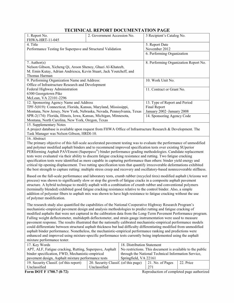
TECHNICAL REPORT DOCUMENTATION PAGE 1. Report No. FHWA-HRT-11-045

2. Government Accession No. 3 Recipient’s Catalog No.

4. Title Performance Testing for Superpave and Structural Validation

5. Report Date November 2012 6. Performing Organization

7. Author(s) Nelson Gibson, Xicheng Qi, Aroon Shenoy, Ghazi Al-Khateeb, M. Emin Kutay, Adrian Andriescu, Kevin Stuart, Jack Youtcheff, and Thomas Harman

8. Performing Organization Report No.

9. Performing Organization Name and Address: Office of Infrastructure Research and Development Federal Highway Administration 6300 Georgetown Pike McLean, VA 22101-2296

10. Work Unit No. 11. Contract or Grant No.

12. Sponsoring Agency Name and Address TPF-5(019): Connecticut, Florida, Kansas, Maryland, Mississippi, Montana, New Jersey, New York, Nebraska, Nevada, Pennsylvania, Texas SPR-2(174): Florida, Illinois, Iowa, Kansas, Michigan, Minnesota, Montana, North Carolina, New York, Oregon, Texas

13. Type of Report and Period Final Report January 2002–January 2008 14. Sponsoring Agency Code

15. Supplementary Notes A project database is available upon request from FHWA Office of Infrastructure Research & Development. The Task Manager was Nelson Gibson, HRDI-10. 16. Abstract The primary objective of this full-scale accelerated pavement testing was to evaluate the performance of unmodified and polymer modified asphalt binders and to recommend improved specification tests over existing SUperior PERforming Asphalt PAVEment (Superpave®) binder performance grading methodologies. Candidate replacement tests were evaluated via their ability to discern fatigue cracking resistance and rutting. Two fatigue cracking specification tests were identified as more capable in capturing performance than others: binder yield energy and critical tip opening displacement. Two rutting specification tests that quantify irrecoverable deformations exhibited the best strength to capture rutting: multiple stress creep and recovery and oscillatory-based nonrecoverable stiffness.

Based on the full-scale performance and laboratory tests, crumb rubber (recycled tires) modified asphalt (Arizona wet process) was shown to significantly slow or stop the growth of fatigue cracks in a composite asphalt pavement structure. A hybrid technique to modify asphalt with a combination of crumb rubber and conventional polymers (terminally blended) exhibited good fatigue cracking resistance relative to the control binder. Also, a simple addition of polyester fibers to asphalt mix was shown to have high resistance to fatigue cracking without the use of polymer modification.

The research study also quantified the capabilities of the National Cooperative Highway Research Program’s mechanistic-empirical pavement design and analysis methodologies to predict rutting and fatigue cracking of modified asphalts that were not captured in the calibration data from the Long-Term Pavement Performance program. Falling weight deflectometer, multidepth deflectometer, and strain gauge instrumentation were used to measure pavement response. The results illustrated that the nationally calibrated mechanistic-empirical performance models could differentiate between structural asphalt thickness but had difficulty differentiating modified from unmodified asphalt binder performance. Nonetheless, the mechanistic-empirical performance ranking and predictions were enhanced and improved using mixture-specific performance tests currently being implemented using the asphalt mixture performance tester. 17. Key Words APT, ALF, Fatigue cracking, Rutting, Superpave, Asphalt binder specification, FWD, Mechanistic-empirical pavement design, Asphalt mixture performance tests

18. Distribution Statement No restrictions. This document is available to the public through the National Technical Information Service, Springfield, VA 22161

19. Security Classif. (of this report) Unclassified

20. Security Classif. (of this page) Unclassified

21. No. of Pages 271

22. Price

Form DOT F 1700.7 (8-72) Reproduction of completed page authorized

ii

SI* (MODERN METRIC) CONVERSION FACTORS APPROXIMATE CONVERSIONS TO SI UNITS

Symbol When You Know Multiply By To Find Symbol LENGTH

in inches 25.4 millimeters mm ft feet 0.305 meters m yd yards 0.914 meters m mi miles 1.61 kilometers km

AREA in2 square inches 645.2 square millimeters mm2

ft2 square feet 0.093 square meters m2

yd2 square yard 0.836 square meters m2

ac acres 0.405 hectares ha mi2 square miles 2.59 square kilometers km2

VOLUME fl oz fluid ounces 29.57 milliliters mL gal gallons 3.785 liters L ft3 cubic feet 0.028 cubic meters m3

yd3 cubic yards 0.765 cubic meters m3

NOTE: volumes greater than 1000 L shall be shown in m3

MASS oz ounces 28.35 grams glb pounds 0.454 kilograms kgT short tons (2000 lb) 0.907 megagrams (or "metric ton") Mg (or "t")

TEMPERATURE (exact degrees) oF Fahrenheit 5 (F-32)/9 Celsius oC

or (F-32)/1.8 ILLUMINATION

fc foot-candles 10.76 lux lx fl foot-Lamberts 3.426 candela/m2 cd/m2

FORCE and PRESSURE or STRESS lbf poundforce 4.45 newtons N lbf/in2 poundforce per square inch 6.89 kilopascals kPa

APPROXIMATE CONVERSIONS FROM SI UNITS Symbol When You Know Multiply By To Find Symbol

LENGTHmm millimeters 0.039 inches in m meters 3.28 feet ft m meters 1.09 yards yd km kilometers 0.621 miles mi

AREA mm2 square millimeters 0.0016 square inches in2

m2 square meters 10.764 square feet ft2

m2 square meters 1.195 square yards yd2

ha hectares 2.47 acres ac km2 square kilometers 0.386 square miles mi2

VOLUME mL milliliters 0.034 fluid ounces fl oz L liters 0.264 gallons gal m3 cubic meters 35.314 cubic feet ft3

m3 cubic meters 1.307 cubic yards yd3

MASS g grams 0.035 ounces ozkg kilograms 2.202 pounds lbMg (or "t") megagrams (or "metric ton") 1.103 short tons (2000 lb) T

TEMPERATURE (exact degrees) oC Celsius 1.8C+32 Fahrenheit oF

ILLUMINATION lx lux 0.0929 foot-candles fc cd/m2 candela/m2 0.2919 foot-Lamberts fl

FORCE and PRESSURE or STRESS N newtons 0.225 poundforce lbf kPa kilopascals 0.145 poundforce per square inch lbf/in2

*SI is the symbol for th International System of Units. Appropriate rounding should be made to comply with Section 4 of ASTM E380. e(Revised March 2003)

iii

TABLE OF CONTENTS

CHAPTER 1. INTRODUCTION .................................................................................................1 BACKGROUND ......................................................................................................................1

Current Asphalt Binder Specifications ................................................................................1 Post-SHRP Full-Scale Validation of Binder Specification ................................................12 Identified Shortcomings with Current Asphalt Binder Specifications ..............................16

PROBLEM STATEMENT ...................................................................................................18 RESEARCH OBJECTIVES .................................................................................................18

CHAPTER 2. EXPERIMENTAL DESIGN AND CONSTRUCTION ...................................19 ASPHALT BINDER SELECTION ......................................................................................19 ARIZONA WET PROCESS CRUMB RUBBER MODIFIED ASPHALT .....................21 MIX DESIGN AND AGGREGATE ....................................................................................22

Gap-Graded Crumb Rubber Mix Design ...........................................................................25 PAVEMENT TEST FACILITY LAYOUT AND CONSTRUCTION .............................25

Hydrated Lime Distribution ...............................................................................................33

CHAPTER 3. ALF LOADING CONDITIONS, FULL-SCALE PERFORMANCE, AND ANALYTICAL PLAN .......................................................................................................37

INTRODUCTION..................................................................................................................37 Wheel and Tire Characteristics ..........................................................................................37 Temperature Control ..........................................................................................................38

MEASURED RUTTING .......................................................................................................38 Transverse Profile and Densification .................................................................................46

MEASURED FATIGUE CRACKING ................................................................................47 Bottom-Up Cracking Evaluation .......................................................................................58 Rutting in Fatigue Sections ................................................................................................59 Anomalous Rutting Performance of Lane 6 ......................................................................62 Rutting in Unbound Layers ................................................................................................69

NUMERICAL AND STATISTICAL CONSEQUENCES OF LAYOUT AND PERFORMANCE ..................................................................................................................70 ANALYTICAL PLAN: HOW WILL ONE CANDIDATE BINDER SPECIFICATION PARAMETER BE COMPARED AGAINST ANOTHER? ..............71

Single Composite Score .....................................................................................................75 Illustration of the Numerical and Statistical Challenges ....................................................76

CHAPTER 4. MECHANISTIC-EMPIRICAL ANALYSIS OF ALF TEST LANES ...........83 INTRODUCTION..................................................................................................................83 FWD ANALYSIS OF UNBOUND LAYER MODULI ......................................................83

Composite Modulus on CAB .............................................................................................84 Back-Calculated Modulus of Pavement Structure .............................................................85 Evaluation of Effective Loading Frequency from FWD ...................................................91 Assessment of Unbound Layer FWD Back-Calculation with Multiple Depth Deflectometers ...................................................................................................................94 Seasonal Monitoring of Pavement Sections with FWD ..................................................105

iv

DIRECT MEASUREMENT OF ASPHALT LAYER MODULUS ................................105 IDT Resilient Modulus of Asphalt ...................................................................................105 Dynamic Modulus of Field Cores and Plant- and Laboratory-Produced Mixtures .........106

MEPDG AND STANDALONE ANALYSES OF ALF PAVEMENTS ..........................113 ALF Wheel and Tire ........................................................................................................114 ALF Temperature and Aging ...........................................................................................115 Other Caveats of the MEPDG and Standalone ................................................................116 HMA Dynamic Modulus Input to MEPDG .....................................................................116 Quantifying Cracking.......................................................................................................121

PRIMARY STRAIN RESPONSE OF PAVEMENTS .....................................................122 Measured Reduction of Modulus .....................................................................................124

PREDICTED PERFORMANCE FROM MEPDG STANDALONE PROGRAM .......127 Influence of Construction Variability on Rutting ............................................................127 Influence of Construction Variability on Fatigue Cracking ............................................131 Assessment of MEPDG Predictive Capability ................................................................134

CONCLUSIONS ..................................................................................................................140

CHAPTER 5. CANDIDATE BINDER PARAMETERS .......................................................143 INTRODUCTION................................................................................................................143 FATIGUE CRACKING ......................................................................................................143

Superpave® Intermediate Temperature ............................................................................143 Superpave® Low-Temperature DT and BBR ..................................................................143 Time Sweep and Stress Sweep ........................................................................................145 Large Strain Time Sweep Surrogate ................................................................................147 Critical Tip Opening Displacement and Essential Work of Fracture ..............................149 Yield Energy ....................................................................................................................152

RUTTING/PERMANENT DEFORMATION BINDER PARAMETERS.....................153 Superpave® High Temperature—Standard and Modified ...............................................154 Multiple Stress Creep and Recovery................................................................................154 Oscillatory-Based Nonrecoverable Stiffness (1/Compliance) .........................................157 Low and Zero Shear Viscosity .........................................................................................161 Material Volumetric Flow Rate .......................................................................................163

CHAPTER 6. MIXTURE PERFORMANCE TESTS ............................................................167 INTRODUCTION................................................................................................................167 MIXTURE TESTS FOR RUTTING ..................................................................................167

HWT ................................................................................................................................167 French PRT ......................................................................................................................169 SST RSCH .......................................................................................................................171 Dynamic Modulus |E*| and Phase Angle .........................................................................176 Flow Number ...................................................................................................................180

MIXTURE TESTS FOR FATIGUE CRACKING ...........................................................194 Texas Transportation Institute Overlay Tester ................................................................194 IDT Strength—ALF Cores ..............................................................................................195 Dynamic Modulus |E*| and Phase Angle .........................................................................196 Axial Cyclic Fatigue ........................................................................................................200 Mixture EWF and Calculated CTOD ..............................................................................206

v

EVALUATION OF MIXTURE TESTS’ ABILITY TO DISCRIMINATE PERFORMANCE ................................................................................................................208

Rutting and Permanent Deformation ...............................................................................208 Cracking and Fatigue .......................................................................................................212

CHAPTER 7. CANDIDATE BINDER SPECIFICATION PARAMETER STRENGTHS .............................................................................................................................215

INTRODUCTION................................................................................................................215 RUTTING/PERMANENT DEFORMATION ..................................................................215

Discussion of Implementability, Purchase Specification Applicability, and Other Caveats ...................................................................................................................219

FATIGUE CRACKING ......................................................................................................219 Discussion of Implementability, Purchase Specification Applicability, and Other Caveats ...................................................................................................................224

CHAPTER 8. CONCLUSIONS AND RECOMMENDATIONS ..........................................227 SUMMARY AND CONCLUSIONS ..................................................................................227

Binder Performance Specification Parameters ................................................................227 RECCOMENDATIONS .....................................................................................................233

APPENDIX. DENT TEST METHOD SPECIFICATION.....................................................235 TITLE ...................................................................................................................................235 SCOPE ..................................................................................................................................235 REFERENCED DOCUMENTS .........................................................................................235 TERMINOLOGY ................................................................................................................235 APPARATUS .......................................................................................................................236 PREPARATION OF SAMPLES ........................................................................................238 TEST PROCEDURES .........................................................................................................238 CALCULATIONS ...............................................................................................................239 REPORTING RESULTS ....................................................................................................240

ACKNOWLEDGEMENTS ......................................................................................................243

REFERENCES ...........................................................................................................................245

vi

LIST OF FIGURES

Figure 1. Flowchart. SHRP asphalt strategy ....................................................................................3 Figure 2. Graph. Dissipated energy during asphalt binder bending beam fatigue ...........................5 Figure 3. Graph. Relationship between strain level and fatigue life in asphalt binder ....................5 Figure 4. Graph. Zaca-Wigmore test road cracking performance and estimated binder properties..........................................................................................................................................6 Figure 5. Graph. SHRP justification for the selection of high-temperature rutting criteria ............7 Figure 6. Chart. Comparison between SHRP mixture flexural beam fatigue and asphalt binder rheology ................................................................................................................................8 Figure 7. Chart. Example of SHRP repeated shear and shear stiffness of mixtures compared against asphalt binder rheology .....................................................................................10 Figure 8. Graph. G* versus sin binder test values for high and low rates of fatigue cracking ...11 Figure 9. Graph. FHWA APT validation of SHRP binder fatigue specification for 4-inch (100-mm) HMA test sections.........................................................................................................12 Figure 10. Graph. FHWA APT validation of SHRP binder fatigue specification for 8-inch (200-mm) HMA test sections.........................................................................................................13 Figure 11. Graph. Post-SHRP rutting binder validation conducted by FHWA .............................14 Figure 12. Graph. RSCH data from NCHRP 9-10.........................................................................16 Figure 13. Graph. Modified binder properties and mixture permanent deformation from NCHRP 9-10 ..................................................................................................................................17 Figure 14. Graph. Modified binder properties and mixture fatigue from NCHRP 9-10 ...............17 Figure 15. Graph. High-intermediate-low PG grades of ALF binders in the experiment .............21 Figure 16. Illustration. Oblique diagram of the test section’s three-dimensional layout ...............26 Figure 17. Graph. Pavement layer profile measured from a trench cut in an ALF test section from past study ...............................................................................................................................27 Figure 18. Photo. Conventional photo of hot mix placement from the back of the paver .............29 Figure 19. Photo. Thermal image of hot mix placement from the back of the paver ....................29 Figure 20. Photo. Characteristic lime nuggets indicating less than desired uniform mixing ........34 Figure 21. Photo. Relative size of lime nuggets ............................................................................34 Figure 22. Illustration. Diagram of 425 tire imprint ......................................................................37 Figure 23. Illustration. LDMA used to measure rut depth .............................................................39 Figure 24. Graph. Rut depths for 4-inch (100-mm) lanes at 147 °F (64 °C) .................................40 Figure 25. Graph. Rut depths for 4-inch (100-mm) lanes at 165 °F (74 °C) .................................41 Figure 26. Graph. Rut depths for 5.8-inch (150-mm) lanes at 147 °F (64 °C) ..............................42 Figure 27. Graph. Rut depths for 5.8-inch (150-mm) lanes at 113 °F (45 °C) ..............................43 Figure 28. Graph. Ranked rut depth of 4-inch (100-mm) lanes at 147 °F (64 °C) and 25,000 passes .................................................................................................................................44 Figure 29. Graph. Ranked rut depth of 5.8-inch (150-mm) lanes at 147 °F (64 °C) and 25,000 passes .................................................................................................................................45 Figure 30. Graph. Surface profile taken in transverse position across the wheel path of a typical zero wander ALF rut .......................................................................................................47 Figure 31. Photo. Typical cracking pattern in loaded ALF wheel paths .......................................48 Figure 32. Graph. Cumulative crack length versus ALF passes in 4-inch (100-mm) 66 °F (19 °C) fatigue loaded sections ......................................................................................................50

δ

vii

Figure 33. Graph. Percent cracked area versus ALF passes in 4-inch (100-mm) 66 °F (19 °C) fatigue loaded sections ......................................................................................................50 Figure 34. Graph. Cumulative crack length versus ALF passes in 5.8-inch (150-mm) 66 °F (19 °C) fatigue loaded sections ......................................................................................................52 Figure 35. Graph. Percent cracked area versus ALF passes in 5.8-inch (150-mm) 66 °F (19 °C) fatigue loaded sections ......................................................................................................52 Figure 36. Photo. Cores from lane 8 (PG70-22) ............................................................................53 Figure 37. Graph. Crack length developed per load cycle at the point of surface crack initiation .........................................................................................................................................54 Figure 38. Graph. Cumulative crack length of 4-inch (100-mm) lanes with interpolated and extrapolated curves ........................................................................................................................55 Figure 39. Graph. Percent cracked area of 4-inch (100-mm) lanes with interpolated and extrapolated curves ........................................................................................................................56 Figure 40. Graph. Arithmetic scale plot of cumulative crack length of 5.8-inch (150-mm) lanes with interpolated and extrapolated curves ............................................................................56 Figure 41. Graph. Semilog scale plot of cumulative crack length of 5.8-inch (150-mm) lanes with interpolated and extrapolated curves ............................................................................57 Figure 42. Graph. Arithmetic scale plot of percent cracked area of 5.8-inch (150-mm) lanes with interpolated and extrapolated curves ............................................................................57 Figure 43. Graph. Semilog scale plot of percent cracked area of 5.8-inch (150-mm) lanes with interpolated and extrapolated curves ............................................................................58 Figure 44. Photo. X-ray computed tomography image slices of an ALF core ..............................58 Figure 45. Photo. Cores taken from lane 1 ....................................................................................59 Figure 46. Graph. Rut depths for 4-inch (100-mm) lanes at 66 °F (19 °C) ...................................60 Figure 47. Graph. Rut depths for 5.8-inch (150-mm) lanes at 66 °F (19 °C) ................................61 Figure 48. Illustration. Schematic layout of ALF lane construction..............................................66 Figure 49. Graph. Particle size distribution of extracted aggregate for lanes 2, 6, and 12 ............69 Figure 50. Diagram. Numerical tree of subsets of available comparative data points ..................70 Figure 51. Equation. Kendall’s tau ................................................................................................72 Figure 52. Graph. Fictitious data with linear regression fit for Kendall’s tau rank correlation example ..........................................................................................................................................74 Figure 53. Graph. Possible permutations of rankings for Kendall’s tau ........................................74 Figure 54. Graph. Continuous area-under-the-curve interpretation for Kendall’s tau ..................75 Figure 55. Equation. t-statistic .......................................................................................................75 Figure 56. Graph. Log-log plot of measured versus predicted dynamic modulus data points from calibrated Witczak predictive equation .................................................................................76 Figure 57. Graph. Arithmetic plot of measured versus predicted dynamic modulus data points from calibrated Witczak predictive equation ......................................................................77 Figure 58. Graph. Variation in composite modulus from FWD on top of CAB ...........................84 Figure 59. Graph. FWD back-calculated CAB modulus from various trial layer configurations ................................................................................................................................86 Figure 60. Graph. FWD back-calculated subgrade modulus from various trial layer configurations ................................................................................................................................86 Figure 61. Graph. Variation of IDT resilient modulus with temperature ......................................87 Figure 62. Graph. Lane 8 PG70-22 asphalt mixture dynamic modulus ........................................92 Figure 63. Graph. Lane 9 SBS 64-40 asphalt mixture dynamic modulus .....................................92 Figure 64. Graph. Lane 10 air-blown asphalt mixture dynamic modulus .....................................93

viii

Figure 65. Graph. Lane 11 SBS-LG asphalt mixture dynamic modulus .......................................93 Figure 66. Graph. Lane 12 terpolymer asphalt mixture dynamic modulus ...................................94 Figure 67. Illustration. Vertical pavement cross section showing anchor points and measurement locations of MDD ....................................................................................................95 Figure 68. Illustration. Layout of lanes 4 and 11 pavement layer configuration for forward-calculation scheme of MDD instrumentation response ...................................................96 Figure 69. Graph. Measured and predicted MDD peak deflection data for lane 4 during FWD loading at 66 °F (19 °C) .......................................................................................................98 Figure 70. Graph. Measured and predicted MDD peak deflection data for lane 11 during FWD loading at 66 °F (19 °C) .......................................................................................................99 Figure 71. Graph. Measured and predicted MDD peak deflection data for lane 4 ALF rolling wheel peak deflections at 50 and 66 °F (10 and 19 °C) ...................................................102 Figure 72. Graph. Measured and predicted MDD peak deflection data for lane 4 ALF rolling wheel peak deflections at 82 and 147 °F (28 and 64 °C) .................................................103 Figure 73. Graph. Measured and predicted MDD peak deflection data for lane 11 ALF rolling wheel peak deflections at 50 and 66 °F (10 and 19 °C) ...................................................104 Figure 74. Graph. Measured and predicted MDD peak deflection data for lane 11 ALF rolling wheel peak deflections at 82 and 147 °F (28 and 64 °C) .................................................105 Figure 75. Graph. |E*| dynamic modulus for field cores versus reduced frequency in log-log scale .................................................................................................................................107 Figure 76. Graph. |E*| dynamic modulus for field cores versus reduced frequency in semilog scale ................................................................................................................................108 Figure 77. Graph. |E*| dynamic modulus for plant-produced mixtures versus reduced frequency in log-log scale ............................................................................................................109 Figure 78. Graph. |E*| dynamic modulus for plant-produced mixtures versus reduced frequency in semilog scale ...........................................................................................................110 Figure 79. Graph. |E*| dynamic modulus for lab-produced mixtures versus reduced frequency in log-log scale ............................................................................................................111 Figure 80. Graph. |E*| dynamic modulus for lab-produced mixtures versus reduced frequency in semilog scale ...........................................................................................................112 Figure 81. Graph. Curves fit to phase angle measured during dynamic modulus test versus reduced frequency .............................................................................................................113 Figure 82. Graph. Rut depth versus pavement age from MEPDG and standalone application ...114 Figure 83. Graph. Asphalt modulus versus pavement age from early run of MEPDG ...............115 Figure 84. Graph. Ratio between predicted dynamic modulus at various air void contents relative to a reference condition ...................................................................................................118 Figure 85. Graph. Extrapolated dynamic modulus in log scale versus reduced frequency .........119 Figure 86. Equation. ALF cracking .............................................................................................121 Figure 87. Equation. Equivalent MEPDG cracking .....................................................................121 Figure 88. Illustration. Layout of an ALF test site with strain gauges ........................................122 Figure 89. Graph. Measured HMA tensile strain versus predicted HMA tensile strain ..............123 Figure 90. Graph. Lane 3 measured tensile strain versus number of ALF passes .......................124 Figure 91. Graph. Lane 8 in-situ measured HMA modulus with seismic analysis versus number of ALF passes .................................................................................................................125 Figure 92. Graph. Lane 10 in-situ measured HMA modulus with seismic analysis versus number of ALF passes .................................................................................................................125 Figure 93. Graph. Lane 11 measured seismic modulus versus number of ALF passes ..............126

ix

Figure 94. Graph. Lane 12 measured seismic modulus versus number of ALF passes ..............127 Figure 95. Graph. Predicted curves of rutting from the MEPDG versus number of ALF passes at 147 °F (64 °C) ...............................................................................................................128 Figure 96. Equation. Empirical rutting distress model used by MEPDG ....................................128 Figure 97. Graph. Percent fatigue cracking predicted from MEPDG standalone program for the as-built scenario ................................................................................................................131 Figure 98. Graph. Percent fatigue cracking predicted from MEPDG standalone program for the as-built with average unbound layer modulus scenario ...................................................132 Figure 99. Graph. Percent fatigue cracking predicted from MEPDG standalone program for the as-designed scenario .........................................................................................................132 Figure 100. Graph. Measured ALF rutting versus MEPDG standalone-predicted rutting for the as-built scenario ................................................................................................................135 Figure 101. Graph. Measured ALF rutting versus MEPDG standalone-predicted rutting for the as-designed scenario .........................................................................................................135 Figure 102. Equation. Cycles to fatigue cracking failure ............................................................137 Figure 103. Graph. Predicted cycles to 7.75 percent cracked area from MEPDG in arithmetic scale versus measured number of cycles ....................................................................138 Figure 104. Graph. Predicted cycles to 7.75 percent cracked area from MEPDG in log scale versus measured number of cycles ...............................................................................138 Figure 105. Graph. Predicted cycles to failure from MEPDG equation in arithmetic scale versus measured number of cycles to surface crack initiation ............................................139 Figure 106. Graph. Failure strain of ALF binders in the low-temperature DT test versus temperature .......................................................................................................................144 Figure 107. Graph. BBR creep m-value of ALF binders versus temperature..............................145 Figure 108. Graph. Typical observations during stress sweep and time sweep tests ..................146 Figure 109. Equation. Stress sweep parameter ............................................................................147 Figure 110. Graph. Complex shear modulus and temperature during 25 percent controlled strain test ......................................................................................................................................148 Figure 111. Graph. Loss modulus and temperature during 25 percent controlled strain test ......148 Figure 112. Illustration. Plan view drawing of DENT test specimen design ..............................150 Figure 113. Photo. DENT test specimens loaded in ductilometer ...............................................150 Figure 114. Graph. Typical raw data from DENT test ................................................................150 Figure 115. Graph. Total work of fracture versus ligament length .............................................151 Figure 116. Equation. Total work of fracture ..............................................................................151 Figure 117. Equation. DENT beta parameter ..............................................................................151 Figure 118. Equation. Approximate CTOD .................................................................................152 Figure 119. Graph. Typical raw data measured during monotonic binder strength test for yield energy ............................................................................................................................153 Figure 120. Graph. Typical applied binder shear stresses during MSCR test .............................155 Figure 121. Graph. Measured raw strain data during MSCR test ................................................155 Figure 122. Graph. Measured raw strain data during entire MSCR test ......................................156 Figure 123. Graph. Creep compliance variation during MSCR test where strain is normalized by applied stress ........................................................................................................156 Figure 124. Equation. Derived estimate of percent unrecovered strain .......................................157 Figure 125. Equation. Derived estimate of unrecovered compliance ..........................................157 Figure 126. Graph. Standard high-temperature Superpave® rutting parameter in log scale versus reduced frequency in log scale ................................................................................158

x

Figure 127. Graph. Oscillatory-based nonrecovered compliance rutting parameter in log scale versus reduced frequency in log scale ..........................................................................159 Figure 128. Graph. Oscillatory-based nonrecovered compliance rutting parameter in arithmetic scale versus temperature in log scale ..........................................................................160 Figure 129. Graph. Trigonometric functions for the standard high-temperature Superpave® rutting parameters and oscillatory-based non-recovered compliance ..........................................160 Figure 130. Graph. Measured nonrecovered compliance from MSCR test versus nonrecovered compliance estimated from shear modulus and phase angle from DSR frequency sweep ..........161 Figure 131. Equation. ZSV ..........................................................................................................162 Figure 132. Graph. Complex viscosity in log scale versus frequency in log scale......................162 Figure 133. Graph. Complex viscosity in log scale versus frequency in log scale......................163 Figure 134. Illustration. Key components of an FMD for determination of MVR .....................164 Figure 135. Graph. MVR versus temperature ..............................................................................164 Figure 136. Graph. HWT rut depth versus wheel tracking cycles ...............................................168 Figure 137. Graph. HWT test cycles to 4-inch (10-mm) rut depth for plant-produced mixtures 169 Figure 138. Photo. Pneumatic wheel in French PRT and rutted test specimen ...........................169 Figure 139. Graph. Rut depth at 60,000 passes in French PRT for plant-produced mixtures .....170 Figure 140. Graph. Permanent shear strain in SST RSCH test versus number of load cycles ....172 Figure 141. Graph. SST RSCH cycles to 2 percent permanent shear strain rut for plant-produced mixtures ..............................................................................................................173 Figure 142. Graph. Permanent shear strain in SST RSCH test for top lifts versus number of load cycles ...............................................................................................................................174 Figure 143. Graph. Permanent shear strain in SST RSCH test for bottom lifts versus number of load cycles ..................................................................................................................174 Figure 144. Graph. Permanent shear strain and number of cycles to 20,000 microstrain ...........175 Figure 145. Graph. Dynamic modulus |E*| at 136 °F (58 °C) and 10 Hz ...................................178 Figure 146. Graph. Dynamic modulus |E*| at 136 °F (58 °C) and 0.1 Hz ..................................179 Figure 147. Graph. |E*|/sin at 136 °F (58 °C) and 10 Hz ..........................................................179 Figure 148. Graph. |E*|/sin at 136 °F (58 °C) and 0.1 Hz .........................................................180 Figure 149. Graph. Permanent axial strain growth in flow number test ......................................181 Figure 150. Illustration. Calculated volumetric permanent strains in a vertical cross sectional plane in the direction of vehicle travel .........................................................................................183 Figure 151. Graph. Axial permanent strain versus number of cycles for mixes with 7 percent air void content, 10 psi (69 kPa) confinement, and 76 psi (523 kPa) axial deviator stress .........184 Figure 152. Graph. Axial permanent strain versus number of cycles for mixes with as-built air void content, 10 psi (69 kPa) confinement, and 120 psi (827 kPa) axial deviator stress .......184 Figure 153. Graph. Axial permanent strain versus number of cycles for mixes with as-built air void content, 1 psi (6.9 kPa) confinement, and 30 psi (207 kPa) axial deviator stress ..........185 Figure 154. Graph. Permanent axial microstrain at 20,000 cycles for ALF mixtures with 7 percent air voids at 10 psi (69 kPa) confinement and 76 psi (523 kPa) axial deviator stress ...186 Figure 155. Graph. Permanent axial microstrain at 5,000 cycles for 4-inch (100-mm) ALF mixtures with as-built air void content at 10 psi (69 kPa) confinement and 120 psi (827 kPa) axial deviator stress .....................................................................................................186 Figure 156. Graph. Permanent axial microstrain at 5,000 cycles for 5.8-inch (150-mm) ALF mixtures with as-built air void content ................................................................................187 Figure 157. Equation. MEPDG empirical rutting model .............................................................187 Figure 158. Equation. Plastic irrecoverable strain .......................................................................188

δ δ

xi

Figure 159. Equation. Equivalence assumed between laboratory performance and MEPDG mechanistic-empirical model formulation ...................................................................................188 Figure 160. Equation. Equating laboratory test power law permanent deformation parameters with MEPDG mechanistic-empirical model formulation .........................................188 Figure 161. Equation. Derivation of recoverable strain for MEDPG mechanistic-empirical permanent deformation model based on applied stress in flow number test and dynamic modulus ........................................................................................................................................188 Figure 162. Graph. Dynamic modulus versus reduced frequency ...............................................189 Figure 163. Equation. Equating laboratory test power law permanent deformation parameters with MEPDG mechanistic-empirical model formulation (continued from figure 160) ....................................................................................................................................189 Figure 164. Equation. Derivation of k1 term for MEPDG mechanistic-empirical model for rutting based on laboratory test conditions ............................................................................189 Figure 165. Graph. Rut depth versus number of ALF passes for best and worst 4-inch (100-mm) ALF lanes....................................................................................................................191 Figure 166. Graph. Rut depth versus number of ALF passes for best and worst 5.8-inch (150-mm) ALF lanes....................................................................................................................192 Figure 167. Graph. Rut depth versus number of ALF passes for 113 °F (45 °C) ALF tests .......192 Figure 168. Graph. Predicted rutting in log scale versus measured rutting in log scale using 10 psi (69 kPa) confined flow number test data at 147 °F (64 °C) ..............................................193 Figure 169. Graph. Predicted rutting in log scale versus measured rutting in log scale using 1 psi (6.9 kPa) confined flow number test data at 147 °F (64 °C) ...............................................193 Figure 170. Illustration. Side view of OT showing fixed and moveable horizontal plates .........194 Figure 171. Graph. IDT strength and corresponding air void content .........................................196 Figure 172. Graph. Dynamic modulus |E*| at 66 °F (19 °C) and 10 Hz .....................................198 Figure 173. Graph. Dynamic modulus |E*| at 66 °F (19 °C) and 0.1 Hz ....................................199 Figure 174. Graph. |E*|sin at 66 °F (19 °C) and 10 Hz .............................................................199 Figure 175. Graph. |E*|sin at 66 °F (19 °C) and 0.1 Hz ............................................................200 Figure 176. Photo. Gyratory-compacted specimen and core test specimen with tension platens glued to each end .............................................................................................................201 Figure 177. Photo. Instrumented tension mounted in universal test machine .............................202 Figure 178. Graph. Dynamic modulus |E*| and phase angle versus number of fatigue cycles during a stress-controlled fatigue test ...............................................................................203 Figure 179. Graph. Dynamic modulus |E*| and phase angle versus number of fatigue cycles during a strain-controlled fatigue test ...............................................................................204 Figure 180. Equation. Energy ratio ..............................................................................................204 Figure 181. Equation. DER ..........................................................................................................204 Figure 182. Equation. Calculation of dissipated energy from phase angle, stress, and strain .....204 Figure 183. Photo. Asphalt mixture DENT specimen for EWF and CTOD characterization .....207 Figure 184. Graph. Fracture energy versus ligament length from mixture DENT testing ..........208 Figure 185. Equation. Composite statistical score .......................................................................209 Figure 186. Illustration. DENT inserts ........................................................................................237 Figure 187. Equation. Total work of fracture calculated from integration of load and displacement data .........................................................................................................................239 Figure 188. Graph. Example wt versus ligament length plot for determining EWF ....................240 Figure 189. Chart. Example reporting sheet ................................................................................241 Figure 190. Graph. Typical load-displacement curves for EWF test ..........................................242

δ δ

xii

LIST OF TABLES

Table 1. Comparison between SHRP mixture flexural beam fatigue and asphalt binder rheology using correlation coefficient, R .........................................................................................9 Table 2. Post-SHRP rutting binder validation conducted by FHWA ............................................14 Table 3. Summary of asphalt binder properties and their location in the ALF test lane configuration ..................................................................................................................................20 Table 4. Recycled crumb rubber particle size in CR-AZ binder ...................................................21 Table 5. Physical properties of CR-AZ binder during blending ....................................................22 Table 6. Laboratory mix design evaluation of volumetrics ...........................................................25 Table 7. Gradation of AASHTO A-4 subgrade .............................................................................27 Table 8. CAB gradation .................................................................................................................28 Table 9. HMA specifications .........................................................................................................30 Table 10. HMA aggregate gradation targets and limits .................................................................30 Table 11. Lime contents measured from ALF lane cores ..............................................................35 Table 12. Rut depths for 4-inch (100-mm) lanes at 147 °F (64 °C) ..............................................39 Table 13. Rut depths for 4-inch (100-mm) lanes at 165 °F (74 °C) ..............................................40 Table 14. Rut depths for 5.8-inch (150-mm) lanes at 147 °F (64 °C) ...........................................41 Table 15. Rut depths for 5.8-inch (150-mm) lanes at 113 °F (45 °C) ...........................................42 Table 16. Ranked rut depth of 4-inch (100-mm) lanes at 147 °F (64 °C) and 25,000 passes .......43 Table 17. Statistical comparison of rut depth of 4-inch (100-mm) lanes at 147 °F (64 °C) and 25,000 passes...........................................................................................................................44 Table 18. Ranked rut depth of 5.8-inch (150-mm) lanes at 147 °F (64 °C) and 25,000 passes ....45 Table 19. Statistical comparison of rut depth of 5.8-inch (150-mm) lanes at 147 °F (64 °C) and 25,000 passes...........................................................................................................................45 Table 20. Cross comparison of rutting in 4- and 5.8-inch (100- and 150-mm) lanes at 25,000 passes .................................................................................................................................46 Table 21. Cumulative crack length in 4-inch (100-mm) fatigue crack sections ............................49 Table 22. Percent cracked area in 4-inch (100-mm) fatigue crack sections ..................................49 Table 23. Cumulative crack length in 5.8-inch (150-mm) fatigue crack sections .........................51 Table 24. Percent cracked area in 5.8- inch (150-mm) fatigue crack sections ..............................51 Table 25. Ranked fatigue cracking of 4-inch (100-mm) lanes at 66 °F (19 °C) ............................55 Table 26. Ranked fatigue cracking of 5.8-inch (150-mm) lanes at 66 °F (19 °C) .........................55 Table 27. Rut depth in 4-inch (100-mm) fatigue crack sections ....................................................60 Table 28. Rut depth in 5.8-inch (150-mm) fatigue crack sections.................................................62 Table 29. Unmodified and modified binders studied by Youtcheff et al .......................................63 Table 30. French PRT rutting performance of binders studied by Youtcheff et al .......................64 Table 31. Flexural beam fatigue performance of binders studied by Youtcheff et al ...................64 Table 32. Stiffness and MSCR of RTFO and extracted terpolymer binder ...................................65 Table 33. FHWA forensic test results for lane 2, 6, and 12 air void content and water absorption from SSD and CoreLok®..............................................................................................67 Table 34. MAMTL forensic test results for lane 2, 6, and 12 air void content, binder content, and water absorption from SSD and CoreLok® .............................................................................68 Table 35. MAMTL forensic test results for lane 2, 6, and 12 extracted aggregate gradation .......69 Table 36. Illustration of the calculation of Kendall’s tau measure of association rank-correlation parameter .............................................................................................................73

xiii

Table 37. Distribution of Kendall’s tau parameter from Monte Carlo simulations .......................78 Table 38. Distribution R from Monte Carlo simulations ...............................................................79 Table 39. Distribution of significance of Kendall’s tau from Monte Carlo simulations ...............79 Table 40. Distribution of regression significance (1 – p-value) from Monte Carlo simulations ...80 Table 41. Modulus back-calculation results for the HMA layers ..................................................88 Table 42. Modulus back-calculation results for the CAB..............................................................89 Table 43. Modulus back-calculation results for the subgrade .......................................................90 Table 44. MDD peak deflections in mm for lane 4 during FWD loading at 66 °F (19 °C) ..........97 Table 45. MDD peak deflections in mm for lane 11 during FWD loading at 66 °F (19 °C) ........97 Table 46. MDD peak deflections in mm for lane 4 during ALF rolling wheel loading at 10,000 lbf (44 kN)........................................................................................................................100 Table 47. MDD peak deflections in mm for lane 11 during ALF rolling wheel loading at 10,000 lbf (44 kN)........................................................................................................................101 Table 48. IDT resilient modulus of plant produced material .......................................................106 Table 49. Air void content of field cores for dynamic modulus ..................................................106 Table 50. Air void content of plant-produced mixture for dynamic modulus .............................109 Table 51. Air void content of lab-produced mixture for dynamic modulus ................................111 Table 52. First-month modulus from MEPDG used in standalone program ...............................120 Table 53. Example of equivalent |E*| temperatures and frequencies using time-temperature superposition ................................................................................................................................121 Table 54. Measured and predicted HMA tensile strains ..............................................................123 Table 55. Predicted 147 °F (64 °C) (40,600 passes) rutting from MEPDG standalone ..............129 Table 56. Predicted 166 °F (74 °C) (40,600 passes) rutting from MEPDG standalone ..............129 Table 57. Predicted 113 °F (45 °C) (302,064 passes) rutting from MEPDG standalone ............130 Table 58. Predicted 66 °F (19 °C) (302,064 passes) rutting from MEPDG standalone ..............130 Table 59. Predicted 66 °F (19 °C) (302,064 passes) fatigue cracking from MEPDG standalone ....................................................................................................................................133 Table 60. Statistical analysis of measured and predicted rutting at different temperatures ........136 Table 61. Statistical analysis of measured and predicted fatigue cracking ..................................140 Table 62. ALF binder standard Superpave® intermediate specification parameters ...................143 Table 63. Low-temperature failure stress, failure strain, and creep m-value ...............................144 Table 64. Summary of time sweeps from Martono and Bahia.(65) ...............................................146 Table 65. Summary of stress sweeps from Martono and Bahia.(65) .............................................147 Table 66. Shenoy’s large strain intermediate stiffness and temperature .....................................149 Table 67. Ranked test results by CTOD with EWF and yield stress ...........................................152 Table 68. Ranked results of yield energy on ALF binders ..........................................................153 Table 69. ALF binder standard and modified Superpave® intermediate specification parameters ....................................................................................................................................154 Table 70. Ranked MSCR nonrecovered compliance ...................................................................157 Table 71. Ranked oscillatory-based nonrecovered compliance ...................................................161 Table 72. Ranked ZSV and LSV .................................................................................................163 Table 73. Ranked MVR and temperature grade from FMD ........................................................165 Table 74. HWT performance of ALF mixtures ...........................................................................168 Table 75. Rut depths from French PRT .......................................................................................170 Table 76. SST RSCH cycles to 2 percent permanent shear strain ...............................................172 Table 77. Summary of SST RSCH ALF core performance .........................................................175 Table 78. Air void content of dynamic modulus specimens ........................................................176

xiv

Table 79. Dynamic modulus and phase angle at 136 °F (58 °C) and 10 Hz ...............................177 Table 80. Dynamic modulus and phase angle at 136 °F (58 °C) and 0.1 Hz ..............................177 Table 81. Summary of AMPT flow number test conditions ........................................................182 Table 82. AMPT flow number performance................................................................................185 Table 83. Modulus, recoverable strain, and permanent strain curve power law coefficients for mix-specific MEPDG rutting predictions ..............................................................................190 Table 84. Mixture-specific MEPDG rutting model coefficients .................................................190 Table 85. ALF 4-inch (100-mm) field core performance in TTI OT.(93) .....................................194 Table 86. IDT strength test results, post-construction (incomplete dataset)................................195 Table 87. IDT strength test results and air void content, bottom lift only (2006 complete dataset) .........................................................................................................................................196 Table 88. Dynamic modulus and phase angle at 66 °F (19 °C) and 10 Hz .................................197 Table 89. Dynamic modulus and phase angle at 66 °F (19 °C) and 0.1 Hz ................................198 Table 90. Initial strain levels of ALF mixtures in stress-controlled fatigue tests ........................202 Table 91. Number of cycles to fatigue failure from different failure criteria ..............................205 Table 92. EWF and CTOD properties of asphalt aggregate mixtures .........................................208 Table 93. Rutting comparisons made between laboratory and full scale ALF performance .......209 Table 94. Statistical comparison of laboratory permanent deformation tests and ALF rutting for 4-inch (100-mm) lanes, including lane 6 terpolymer .................................................210 Table 95. Statistical comparison of laboratory permanent deformation tests and ALF rutting for 4-inch (100–mm) lanes, excluding lane 6 terpolymer ................................................210 Table 96. Statistical comparison of laboratory permanent deformation tests and ALF rutting for 5.8-inch (150-mm) lanes .............................................................................................211 Table 97. Fatigue cracking comparisons made between laboratory and full-scale ALF performance .................................................................................................................................212 Table 98. Statistical comparison of laboratory fatigue cracking tests and ALF fatigue, 4-inch (100-mm) lanes .................................................................................................................213 Table 99. Statistical comparison of laboratory fatigue cracking tests and ALF fatigue, 5.8-inch (150-mm) lanes ..............................................................................................................214 Table 100. Evaluation of correct or incorrect trends among binder properties, mixture properties, and 4-inch (100-mm) ALF rutting .............................................................................216 Table 101. Evaluation of correct or incorrect trends among binder properties, mixture properties, and 5.8-inch (150-mm) ALF rutting ..........................................................................217 Table 102. Ranking of binder high-temperature rutting parameters with lane 6 (terpolymer)....218 Table 103. Ranking of binder high-temperature rutting parameters without lane 6 (terpolymer) .................................................................................................................................218 Table 104. Evaluation of correct or incorrect trends between binder properties, mixture properties, and 4-inch (100-mm) ALF fatigue cracking ................................................220 Table 105. Ranked binder fatigue cracking parameters from 4-inch (100-mm) ALF lanes ........221 Table 106. Ranked binder fatigue cracking parameters from 5.8-inch (150 mm) ALF lanes with lane 9 (SBS 64-40) ...............................................................................................................221 Table 107. Ranked binder fatigue cracking parameters from 5.8-inch (150-mm) ALF lanes without lane 9 (SBS 64-40) ........................................................................................222 Table 108. Description of Ontario binders and physical properties ............................................222 Table 109. Total number of crack performance of Ontario pavement test sections ....................223 Table 110. Total crack length performance of Ontario pavement test sections ...........................223 Table 111. Total transverse crack performance of Ontario pavement test sections ....................223

xv

Table 112. Comparison between binder fatigue cracking test and Ontario total number of cracks ...........................................................................................................................................224 Table 113. Comparison between binder fatigue cracking test and Ontario total length of cracks ...........................................................................................................................................224 Table 114. Comparison between binder fatigue cracking test and Ontario length of transverse cracks ..........................................................................................................................224

xvi

LIST OF ACRONYMS AND ABBREVIATIONS

AASHTO American Association of State Highway and Transportation Officials

AC Asphalt concrete

ALF Accelerated load facility

AMPT Asphalt mixture performance tester

ANOVA Analysis of variance

APT Accelerated pavement testing

BBR Bending beam rheometer

CAB Crushed aggregate base

COV Coefficient of variation

CR-AZ Arizona wet process crumb rubber modified

CR-TB Terminally blended crumb rubber modified

CTOD Critical tip opening displacement

DENT Double edged notched tension

DER Dissipated energy ratio

DSR Dynamic shear rheometer

DT Direct tension

EICM Enhanced Integrated Climatic model

ETG Expert task group

EWF Essential work of fracture

FHWA Federal Highway Administration

FMD Flow measurement device

FWD Falling weight deflectometer

GPS General Pavement Study

HMA Hot mix asphalt

xvii

HWT Hamburg wheel tracking

IDT Indirect tension

LDMA Layer deformation measurement assembly

LSV Low shear viscosity

LTPP Long-Term Pavement Performance

LVDT Linear variable differential transformer

MAMTL Mobile Asphalt Materials Testing Laboratory

MDD Multiple depth deflectometer

MEPDG Mechanistic-Empirical Pavement Design Guide

MTD Material transfer device

MSCR Multiple stress creep and recovery

MVR Material volumetric rate

NCHRP National Cooperative Highway Research Program

OT Overlay tester

PAV Pressure-aging vessel

PG Performance grade

PRT Pavement rut tester

PSPA Portable seismic pavement analyzer

PTF Pavement test facility

RMSE Root mean square error

RSCH Repeated shear at constant height

RTFO Rolling thin film oven

SBS Styrene-butadiene-styrene

SBS-LG Linear grafted SBS

SHRP Strategic Highway Research Program

xviii

SPS Specific Pavement Study

SPT Simple performance test

SSD Saturated surface dry

SST Simple shear tester

Superpave® SUperior PERforming Asphalt PAVEment

TCE Trichloroethylene

TFHRC Tuner-Fairbank Highway Research Center

TPF Transportation Pooled Fund

TTI Texas Transportation Institute

VECD Viscoelastic continuum damage

VFA Voids filled with asphalt

VMA Voids in mineral aggregate

ZSV Zero shear viscosity

1

CHAPTER 1. INTRODUCTION

BACKGROUND

The United States produces hundreds of millions of tons of hot mix asphalt (HMA) each year for pavement construction and maintenance. Although the asphalt weighs less and represents a smaller proportion of the HMA mixture, the liquid asphalt binder component is more costly than the stone aggregate component, translating to billions of dollars spent annually. Asphalt binders for HMA are purchased, graded, and verified using the SUperior PERforming Asphalt PAVEment (Superpave®) performance grade (PG) system developed by the Strategic Highway Research Program (SHRP).

Current Asphalt Binder Specifications

The aim of the Superpave® PG system and asphalt binder specifications is to ensure acceptable performance of flexible asphalt pavements in three distinct temperature or seasonal regimes, each associated with a different distress. The assurance of acceptable performance comes with the following requirements:

• The asphalt binder must be part of a valid asphalt-aggregate mixture design.

• The HMA layer must be configured in a valid pavement structural design.

• The pavement must be constructed without any deficiencies.

State transportation agencies specify PG binder using specifications adopted by the American Association of State Highway and Transportation Officials (AASHTO). AASHTO M 320, Standard Specification for Performance-Graded Asphalt Binder, assigns three temperature grades to a particular asphalt binder using the following three tests:(2)

• AASHTO T 313: Standard Method of Test for Determining the Flexural Creep Stiffness of Asphalt Binder Using the Bending Beam Rheometer (BBR).(3)

• AASHTO T 314: Standard Method of Test for Determining the Fracture Properties of Asphalt Binder in Direct Tension (DT).(4)

• AASHTO T 315: Standard Method of Test for Determining the Rheological Properties of Asphalt Binder Using a Dynamic Shear Rheometer (DSR).(5)

Both AASHTO T 313 and AASHTO T 314 measure material properties intended to control low-temperature thermal cracking performance.(3,4) This is not within the scope of this research. AASHTO T 315 measures material properties intended to control both high-temperature rutting and intermediate-temperature fatigue cracking distresses. The rheological properties of asphalt binders characterized using a dynamic shear rheometer (DSR) are the viscoelastic (complex) shear modulus, |G*|, and viscoelastic phase angle, . Temperature and rate of loading affect these rheological properties, which is why they are considered viscoelastic in nature. Increasing temperature decreases asphalt binder stiffness while increasing the viscoelastic phase angle and

δ

2

vice versa. Decreasing the rate of loading has the same effect as increasing temperature. SHRP’s Asphalt Research Program recommended combinations of the shear modulus and phase angle as specification criteria for rutting and fatigue cracking.(6)

SHRP was initiated to increase the life of pavements and decrease life-cycle costs and maintenance requirements. Asphalt research focused on delivering two products: a performance-based binder specification and an asphalt aggregate mixture design and analysis system. The research was broken into the following contracts:(7)

• A-001: Improved Asphaltic Materials, Experiment Design, Coordination, and Control of Experimental Materials.

• A-002A: Binder Characterization and Evaluation.

• A-003A: Performance-Related Testing and Measure of Asphalt-Aggregate Interaction and Mixtures.

• A-003B: Fundamental Properties of Asphalt-Aggregate Interaction Including Adhesion and Absorption.

• A-004: Asphalt Modification.

• A-005: Performance Model and Validation of Test Results.

• A-006: Performance-Based Specifications for Asphalt Aggregate Mixtures.

To achieve the desired products, the research was broken into four distinct phases. The first phase was conceptualization, identifying candidate physiochemical phenomena in binders and mechanical properties of mixtures that govern asphalt pavement performance. The second phase was definition, defining the asphalt binder properties that would be validated against laboratory accelerated mixture performance tests and, to a lesser degree, with full-scale accelerated pavement testing (APT). These activities were considered a first-stage validation. At the same time, tests suitable for specifications were developed. This phase was followed by the validation phase, during which field performance data were used to complete the first-stage validation of binder and mixture properties that were judged to have a strong effect on pavement performance in the definition phase. This was considered the second-stage validation. The last stage was adoption, where the implementation of binder and mixture specifications begins. Ultimately, the third-stage validation would come from Long-Term Pavement Performance (LTPP) Specific Pavement Study (SPS)-9 test sections.

SHRP contracts A-002A, A-003A, and A-005 had the greatest influence on research and recommendations leading to the current asphalt binder PG specifications. Contract A-002A was tasked with identifying chemical and physical properties of asphalt binders that were associated with performance and developing specification tests for these properties. Contracts A-003A and A-005 supported A-002A to provide validation. Contract A-003A developed standard laboratory asphalt-aggregate mixture tests based on properties identified in A-002A. Contract A-005 provided the basis for criteria and limits to refine asphalt binder and mixture specification tests

3

from field performance. The interaction among contracts is shown graphically in figure 1, which is reproduced from the SHRP Asphalt Research Program strategic plan.(7)

Figure 1. Flowchart. SHRP asphalt strategy.(7)

SHRP contract A-002A was comprehensive and focused on a molecular microstructural chemical model for the asphalt binder, aging and oxidative mechanisms, and physical rheological properties that are the subject of this research. SHRP A-367 describes physical rheological properties for specification tests and presents why various empirical techniques are inferior to fundamental viscoelastic properties, which are the basis for the current Superpave® PG specifications.(6) The primary advantage of fundamental viscoelastic rheological properties of asphalt binder is the ability to account for temperature effects, aging effects, shear rate, and viscosity effects.

SHRP A-369 explains why and how the fundamental viscoelastic rheological properties were developed and chosen and, importantly, describes limits and criteria for those properties in the current practice found in AASHTO T 315.(8,5)

With respect to fatigue cracking, the SHRP researchers responsible for developing specification tests were aware of the complicated fundamental fatigue and fracture phenomena associated with asphalt cracking. These include stress concentrations found at the leading edge of crack tips and

A-002A/A-003AIdentify CompositionQuantify Composition Develop Physical Tests

Correlation Composition and Physical Properties

A-004Validate tests for modified

binder

A-003AValidate A-002A with simulative large scale lab tests (Phase 1)

A-005Develop &

validate models

A-005Validate A-002A

with field data (Phase 2)

A-001Develop binder

specification and protocols

A-002A/A-003AIdentify CompositionQuantify Composition Develop Physical Tests

Correlation Composition and Physical Properties

A-004Validate tests for modified

binder

A-003AValidate A-002A with simulative large scale lab tests (Phase 1)

A-005Develop &

validate models

A-005Validate A-002A

with field data (Phase 2)

A-001Develop binder

specification and protocols

4

mathematics regarding the propagation of those cracks as well as the inelastic conditions that influence fracture mechanics theories. The researchers identified the presence of plasticity and viscoelasticity and the energy dissipation at intermediate temperatures where fatigue cracking is assumed the dominant distress. Relationships between fatigue and fracture did not exist because the profession lacked a convenient test for asphalt binder fatigue. Fracture was explicitly explored with direct tension (DT) fracture tests for low-temperature cracking. Master curves of failure stress and failure strain over wide ranges of temperature and strain rate were developed as a possible means to extend DT fracture testing from low temperatures (thermal transverse cracking) to intermediate temperatures (fatigue, alligator cracking, etc.). However, doing so would require a transition from the brittle state at low temperatures to a combined ductile-brittle state at warmer temperatures.

Explicit justification for a practical surrogate for advanced fundamental tests was that fatigue tests are too lengthy for practical specifications and fatigue phenomena in the field occur over a broad range of temperatures and stress levels depending on traffic and location within the pavement structure. Fundamental fatigue tests had to be conducted to support the choice of a surrogate test. SHRP researchers utilized reduced-scale three-point bending beam geometries of composite aluminum metal and asphalt binder. Strain magnitudes of the beam undergoing fatigue were between 5,200 and 1,400 microstrain (0.52 and 0.14 percent), and the temperature range was -22 to 32 °F (-30 to 0 °C). It is interesting to note that such classical cyclic fatigue characterization tests are contemporarily conducted in parallel plate geometry using DSR at more intermediate temperatures, as discussed in later sections of this report. Failure was defined as the appearance of a crack in the asphalt beam.

A number of phenomena were confirmed. First, the larger the induced repeated strain in the fatigue test, the fewer number of cycles to achieve failure. Second, the ratio of the energy lost due to viscoelasticity and fatigue damage in a given cycle compared to the total energy input for a given cycle remains constant as cycles increase during the fatigue test but increase dramatically at the end when damage dominates. An example of this from SHRP research is shown in figure 2. The second observation was that energy dissipated is a strong indicator of fatigue damage. Analytical closed-form solutions based on dissipated energy were derived to equate the number of cycles to the strain level and total dissipated energy for an entire fatigue test. Experiment and theory matched reasonably well, as shown in figure 3. DSR instruments were introduced in the SHRP project, and dissipated energy was related to the parameter |G*|× sin . This parameter was ultimately selected as the specification controlling fatigue cracking. Justification for the parameter criteria initially set at 435 psi (3 MPa) was made utilizing data from the Zaca-Wigmore road test built in the mid to late 1950s to assist the California Department of Highways in evaluating penetration binder specifications and durability.(9,10) Figure 4 shows the data where sections with larger |G*| × sin values exhibited greater amounts of cracking. SHRP researchers utilized this data to justify the limit of 435 psi (3 MPa) for |G*| × sin . However, the Federal Highway Administration (FHWA) Asphalt Expert Task Group (ETG) suggested increasing the limit to 725 psi (5 MPa), which can be found in the current practice specification of AASHTO M 320.(2)

δ

δ

δ

5

Figure 2. Graph. Dissipated energy during asphalt binder bending beam fatigue.(8)

Figure 3. Graph. Relationship between strain level and fatigue life in asphalt binder.(8)

6

Figure 4. Graph. Zaca-Wigmore test road cracking performance and estimated

binder properties.(6)

With respect to rutting specifications and criteria, SHRP A-369 proposed that asphalt binders exhibit both recoverable and irrecoverable components of viscoelastic deformations and that it is the irrecoverable component that contributes to the permanent deformation and rutting observed in full-scale pavements.(8) To explore these phenomena, a unique apparatus and asphalt binder sample test configuration was developed. An actuator provided repeated loading with rest periods to a piston that penetrated a sample of asphalt binder controlled at a fixed temperature. The apparatus measured the recoverable and irrecoverable deformations. The rest period allowed the recoverable deformations to attenuate from the total deformations, leaving behind a permanent or plastic deformation before the next load cycle. The experimental program measured these plastic and permanent deformations on a series of asphalt binders, some unmodified and some polymer modified. The SHRP research found that large permanent deformations grew in a nonlinear fashion. More practical indentation tests were explored as an alternative; however, the material response of interest was not necessarily the plastic deformations but the manner in which stresses relax in asphalt binder from a monotonic indentation. This characterization was done at cooler-than-ideal high-temperature rutting conditions. In other words, the researchers were looking to measure fundamental linear viscoelastic relaxation modulus. All previous mechanical characterization instruments were abandoned as SHRP research adopted DSRs, which generate dynamic data that can be converted to time-domain data and provide the relaxation of interest.

SHRP A-367 indicates that originally, the “viscous component of stiffness” was found not to correlate with mixture data.(6) The type of mixture data and quality of the correlation were not provided in the final reports. Ultimately, the loss compliance was selected as the ideal specification parameter, which could be calculated from the DSR instrument as the shear modulus divided by the sine of the phase angle, |G*|/sin . Justification for this parameter shown in figure 5 came from personal communication that correlated non-descript wheel tracking tests of six unknown mixture data points with loss compliance (|G*|/sin ).

δ

δ

7

1 Pa = 0.000145 psi 1 mm = 0.039 inches

Figure 5. Graph. SHRP justification for the selection of high-temperature rutting criteria.(7)

SHRP Binder Parameter Validation with Mixture Characterization

Asphalt binder parameters proposed by the SHRP A-002A contract were tested and validated against the extensive and comprehensive laboratory mixture tests conducted by the SHRP A-003A contract. SHRP A-404 and SHRP A-515 provide an exhaustive description of the various tests explored for fatigue characterization and rutting/permanent deformation.(11,12) Ultimately, flexural beam fatigue tests and simple shear testing were selected as the ideal laboratory characterization tests. A summary of the comparison between binder properties and mixture properties is given in SHRP A-398 and also in a more concise summary by Leahy et al.(13,14)

To evaluate the fatigue binder specification, mixtures from eight SHRP core asphalt binders (unmodified) and two SHRP core aggregates were tested at two air void levels and repeated strain levels. A total of 128 specimens were tested. The experimental design examined the effects of binder type, aggregate type, density, and binder-aggregate and binder-density interactions. Binder type was found to have the strongest influence on fatigue life, as defined by 50 percent reduction in modulus. However, researchers found that other factors were also significant contributors and could not be considered negligible. Comparisons were made between the fatigue life of the mixtures and binders. To eliminate interaction effects from the other variables, four scenarios (the combinations of the two aggregates and two density levels) were analyzed. Cyclic strain level was averaged. An example of one of the SHRP scatter plots for fatigue life versus binder property is shown in figure 6, but figures for dissipated energy and other properties were also provided. Each comparison has eight data points, and Pearson’s correlation coefficient, R, was calculated and is given in table 1. (Note that this is not the coefficient of determination, R2.) The fatigue life, in general, had a good relationship with the logarithmic value of the specification |G*| × sin equal to the loss modulus G'', the logarithmic value of the complex stiffness |G*|, and the logarithmic value of the storage modulus G' equal to |G*| × cos . For

δ δ

8

binders with the same specification parameter |G*| × sin , stiffness could have as much as twice the fatigue life depending on the aggregate and density. The SHRP researchers noted that the phase angle had little effect and that any of the stiffness relationships could be used. However, it was recognized that modified asphalt could benefit from the sin term.

RD = Quarried,100 percent crushed aggregate. RH = Partially crushed river gravel.

Figure 6. Chart. Comparison between SHRP mixture flexural beam fatigue and asphalt binder rheology.(13)

δ

δ

9

Table 1. Comparison between SHRP mixture flexural beam fatigue and asphalt binder rheology using correlation coefficient, R.(13)

Mix Property Flexural Stiffness Fatigue Life

Dissipated Energy

Aggregate RD, 4 percent air voids Log (|G*|•sin ) 0.906 -0.535 -0.32 Log |G*| 0.904 -0.474 -0.241 Log G' 0.888 -0.401 -0.149 Log(tan ) -0.564 -0.156 -0.456

Aggregate RD, 7 percent air voids Log (|G*|•sin ) 0.905 -0.935 -0.672 Log |G*| 0.909 -0.927 -0.622 Log G' 0.897 -0.915 -0.568 Log(tan ) -0.606 0.578 0.062

Aggregate RH, 4 percent air voids Log (|G*| × sin ) 0.951 -0.951 -0.806 Log |G*| 0.946 -0.945 -0.76 Log G' 0.926 -0.933 -0.707 Log(tan ) -0.571 0.6 0.175

Aggregate RH, 7 percent air voids Log (|G*| × sin ) 0.952 -0.927 -0.925 Log |G*| 0.935 -0.944 -0.935 Log G' 0.902 -0.952 -0.935 Log(tan ) -0.473 0.753 0.692

RD = Quarried 100 percent crushed aggregate. RH = Partially crushed river gravel.

SHRP conducted an analysis that expanded upon the mixture effects (i.e., air voids and density). The impact of pavement structural configuration (i.e., stiff versus soft or thick versus thin layers) was explored, as well. The results of the beam fatigue tests were used to calibrate the generic model for fatigue life as a function of the inverse of the tensile strain magnitude. Two scenarios were considered: (1) an asphalt concrete (AC) layer on aggregate base over a subgrade and (2) a thicker AC layer on a softer subgrade. The fatigue lives of the fictitious pavements predicted from the equation were compared against the binder properties. The relationships between binder and pavement performance were weaker than the relationships between binder and laboratory test fatigue life shown in table 1 and figure 6. In addition, the trends with lab-mix specimens were opposite the trends with binder. Notably, the generic model for pavement structure fatigue life did not include stiffness, as does the current empirical equation in the National Cooperative Highway Research Program (NCHRP) 1-37A, Mechanistic-Empirical Pavement Design Guide (MEPDG) methodology.(1) The SHRP analysis shows that structural configuration of pavement has a significant contribution to overall performance and, depending on the situation, may override the choice of asphalt binder.

The approach used with respect to rutting was similar to that used for fatigue characterization. Wheel tracking tests and laboratory shear tests were conducted. Sixteen asphalt binders and two aggregates were used to make samples at two air void levels for wheel tracking tests. Nine asphalt binders and two aggregates were used to make samples at two air void contents for the laboratory shear tests. Statistical analysis of variance (ANOVA) was conducted to assess the

δ

δ

δ

δ

δ

δ

δ

δ

10

proportional effect of binder type, aggregate type, density, and the interaction between binder and aggregate. In contrast to the fatigue analysis, there were almost equal contributions from aggregate, binder, and binder-aggregate interaction for the wheel tracking tests but less so for density. Statistical findings were similar for the laboratory repeated shear testing, except with a bit larger error than wheel tracking. As with the fatigue analysis, the laboratory wheel tracking and shear tests were compared to the characteristics of the binder only by separating the data into the four combinations of the two aggregates and two density levels. Comparative plots and correlation calculations of the binder properties against wheel tracking and laboratory repeated shear were conducted similar to the fatigue characterization. Typical results from SHRP are shown in figure 7. Significant scatter was observed, with inconsistent trends at times being positive or negative for a particular scenario of aggregate type, density, and laboratory characteristics. The SHRP researchers concluded that binder properties can be overridden by aggregate properties. One comment from the SHRP researchers was that the tests were conducted at the relatively low temperature of 104 °F (40 °C), and higher temperature tests could emphasize the effect of binder, as in this Transportation Pooled Fund (TPF) research.

Figure 7. Chart. Example of SHRP repeated shear and shear stiffness of mixtures

compared against asphalt binder rheology.(13)

11

SHRP Field Validation

SHRP contract A-005 provided more near-term validation of the selected binder specifications until the results from the LTPP program could yield sufficient data. The research was intended to provide documented field performance data to help set criteria to the parameters determined in SHPR contract A-003. SHRP A-357 provides empirical validation of the binder specifications for load-related distresses fatigue cracking and rutting.(15)

SHRP General Pavement Study (GPS) test sites were used by the researchers. Asphalt binder from 29 sections was extracted and characterized for comparison. The 29 sections came from Alabama, Alaska, Arizona, Arkansas, California, Colorado, Florida, Idaho, Illinois, Kentucky, Maine, Michigan, Mississippi, Nevada, New Jersey, New Mexico, Oklahoma, Tennessee, Utah, and Quebec. Two types of pavement performance prediction software, FLEXPASS and Texas Flexible Pavement System, were used to calculate predicted rutting and cracking distresses based on material properties measured on the mixtures in the laboratory and back-calculated properties from nondestructive techniques. The ratio of measured to predicted distresses was calculated. Ratios larger than 1.0 were categorized as high, and ratios smaller than 1.0 were categorized as low.

The logic for this analysis was to eliminate contributions from supporting layers and emphasize contributions from the AC layer. Binder |G*| was plotted against binder phase angle, the two components of the rutting and fatigue cracking specification parameters. Each point was identified with its corresponding high or low ratio of predicted versus measured distress. The graph for fatigue cracking in the GPS test sections shows no clear trends, with the high and low points interspersed among each other (see figure 8). The quality of the scatter plot is similar for rutting. The conclusion drawn by SHRP A-005 researchers was that no binder specification by itself can explain field performance.

1 kPa = 0.145 psi

Figure 8. Graph. G* versus sin binder test values for high and low rates of fatigue cracking.(13)

δ

12

Post-SHRP Full-Scale Validation of Binder Specification

FHWA APT

FHWA provided APT to validate the newly developed SHRP binder specifications |G*| × sin and |G*|/sin .(16–18) Two unmodified asphalts with high, intermediate, and low PG temperature grades of 58, 9, and -34 and 64, 17, and -22 were used in a single mix design with 4- and 8-inch (100- and 200-mm)-thick asphalt layers, respectively. Test pavements were trafficked by an accelerated load facility (ALF) at 50, 66, and 82 °F (10, 19, and 28 °C).

The fatigue experiment was designed to evaluate whether stiffer binders defined by |G*| × sin and, thus, stiffer mixtures, performed better in thicker asphalt layers while softer, more compliant binders defined by lower |G*| × sin and, thus, softer mixtures, provided better fatigue cracking resistance in thinner asphalt pavements. The experiment also tested whether there was a pessimum temperature for fatigue cracking. In other words, there should be less fatigue cracking at temperate cooler and warmer temperatures than at some critical intermediate temperature.

These fatigue phenomena are partially confirmed in figure 9 and figure 10, where the middle test temperature of 66 °F (19 °C) required fewer passes to produce cracks than did 50 or 82 °F (10 or 28 °C). However, binder |G*| × sin only partly explained the performance in the thinner pavement, where strain control phenomena were believed to dominate. This is not a departure from classical pavement engineering. At the intermediate 66 °F (19 °C) temperature for both 4- and 8-inch (100- and 200-mm)-thick pavements, the binder with the stiffer |G*|•sin performed better, contrary to the intent of the specification. The researchers suggest that the loss compliance used for high-temperature binder specifications, |G*|/sin , is associated with stress control fatigue phenomena and |G*| × sin is associated with strain control fatigue phenomena and that stress control |G*|/sin should be used to grade fatigue performance for thicker pavements.

°F = 1.8(°C) + 32

Figure 9. Graph. FHWA APT validation of SHRP binder fatigue specification for 4-inch (100-mm) HMA test sections.(16)

δ δ

δ

δ

δ

δ

δ δ

δ

100,000

1,000

14,000

50,000

10,000

20,000

-

20,000

40,000

60,000

80,000

100,000

120,000

28C 19C 10CALF Test Temperature

Num

ber o

f ALF

Whe

el P

asse

s Fo

r Fi

rst C

rack

to A

ppea

r At S

urfa

ce

"Softer" PG 58•9•-34 "Stiffer" PG64•17•-22

13

°F = 1.8(°C) + 32

Figure 10. Graph. FHWA APT validation of SHRP binder fatigue specification for 8-inch (200-mm) HMA test sections.(16)

Rutting was evaluated at multiple temperatures between 115 and 169 °F (46 and 76 °C) on five asphalt binders. Three binders were unmodified: AC-5, AC-10, and AC-20, with high-temperature grades of PG58, PG64, and PG70, respectively. Two binders, Novophalt and Styrelf, were modified asphalts with high-temperature grades of PG76 and PG82. The number of wheel passes to achieve 0.8-inch (20-mm) rut depth was used to assess the validity of the parameter |G*|/sin . However, the parameter at a slower frequency of 2.25 radians/s in the DSR was chosen instead of the standard 10 radians/s because of the slow speed of the FHWA ALF.

As shown in table 2, binders were characterized at three temperatures, and test lanes were loaded at those same temperatures, depending on the stiffness of the binders. For the polymer modified asphalts, the rutting was quite low, and thus, power law models were fit to the measured rutting versus wheel pass data to extrapolate to the 0.8-inch (20-mm) rut depth criteria. A very broad range in wheel passes was found and is presented in figure 11 using a semilogarithmic scale.

300,000

25,000

250,000

350,000

150,000

220,000

-

50,000

100,000

150,000

200,000

250,000

300,000

350,000

400,000

28C 19C 10CALF Test Temperature

Num

ber o

f ALF

Whe

el P

asse

s Fo

r Fi

rst C

rack

to A

ppea

r At S

urfa

ce

"Softer" PG 58•9•-34

"Stiffer" PG64•17•-22

δ

14

Table 2. Post-SHRP rutting binder validation conducted by FHWA.(18)

Binder

Wheel Passes to 20-mm

Rut Depth Temperature

(°C)

|G*|/sin at 2.25 radians/s

(Pa)

AC-5 (PG58)

192,000 46 4,061 1,950 52 1,557

670 58 664

AC-10 (PG64)

83,000 46 8,865 21,720 52 3,329 1,900 58 1,384

AC-20 (PG70)

161,400 52 6,744 2,740 58 2,702 7,000 64 1,175

Novophalt (PG76)

6,000,000 58 6,826 340,000 70 1,304

1,900,000 76 642

Styrelf (PG82)

220,000 58 13,710 98,300 70 4,435

236,000 76 2,381 1 mm = 0.039 inches °F = 1.8(°C) + 32 1 Pa = 0.000145 psi

1 Pa = 0.000145 psi 1 mm = 0.039 inches Figure 11. Graph. Post-SHRP rutting binder validation conducted by FHWA.(18)

δ

100

1,000

10,000

100,000

1,000,000

10,000,000

- 2,000 4,000 6,000 8,000 10,000 12,000 14,000 16,000

Binder G*/sin(δ) at 2.25 rad/sec (Pa)

Whe

el P

asse

s to

20m

m R

ut D

epth

Unmodified AC BindersModified Binders

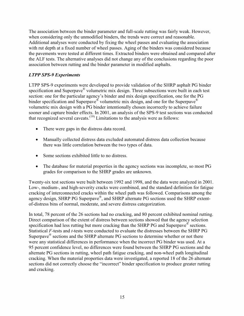
15

The association between the binder parameter and full-scale rutting was fairly weak. However, when considering only the unmodified binders, the trends were correct and reasonable. Additional analyses were conducted by fixing the wheel passes and evaluating the association with rut depth at a fixed number of wheel passes. Aging of the binders was considered because the pavements were tested at different times. Extracted binders were obtained and compared after the ALF tests. The alternative analyses did not change any of the conclusions regarding the poor association between rutting and the binder parameter in modified asphalts.

LTPP SPS-9 Experiments

LTPP SPS-9 experiments were developed to provide validation of the SHRP asphalt PG binder specification and Superpave® volumetric mix design. Three subsections were built in each test section: one for the particular agency’s binder and mix design specification, one for the PG binder specification and Superpave® volumetric mix design, and one for the Superpave® volumetric mix design with a PG binder intentionally chosen incorrectly to achieve failure sooner and capture binder effects. In 2001, an analysis of the SPS-9 test sections was conducted that recognized several caveats.(19) Limitations to the analysis were as follows:

• There were gaps in the distress data record.

• Manually collected distress data excluded automated distress data collection because there was little correlation between the two types of data.

• Some sections exhibited little to no distress.

• The database for material properties in the agency sections was incomplete, so most PG grades for comparison to the SHRP grades are unknown.

Twenty-six test sections were built between 1992 and 1998, and the data were analyzed in 2001. Low-, medium-, and high-severity cracks were combined, and the standard definition for fatigue cracking of interconnected cracks within the wheel path was followed. Comparisons among the agency design, SHRP PG Superpave®, and SHRP alternate PG sections used the SHRP extent-of-distress bins of normal, moderate, and severe distress categorization.

In total, 78 percent of the 26 sections had no cracking, and 80 percent exhibited nominal rutting. Direct comparison of the extent of distress between sections showed that the agency selection specification had less rutting but more cracking than the SHRP PG and Superpave® sections. Statistical F-tests and t-tests were conducted to evaluate the distresses between the SHRP PG Superpave® sections and the SHRP alternate PG sections to determine whether or not there were any statistical differences in performance when the incorrect PG binder was used. At a 95 percent confidence level, no differences were found between the SHRP PG sections and the alternate PG sections in rutting, wheel path fatigue cracking, and non-wheel path longitudinal cracking. When the material properties data were investigated, a reported 18 of the 26 alternate sections did not correctly choose the “incorrect” binder specification to produce greater rutting and cracking.

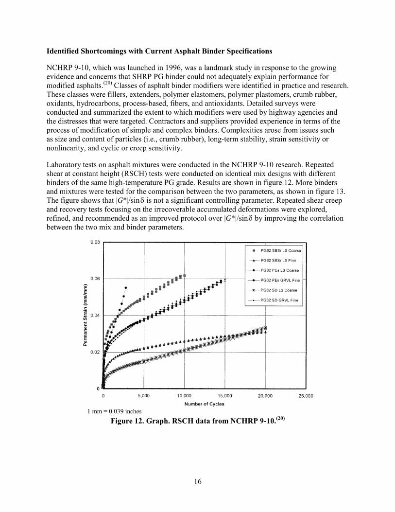
16

Identified Shortcomings with Current Asphalt Binder Specifications

NCHRP 9-10, which was launched in 1996, was a landmark study in response to the growing evidence and concerns that SHRP PG binder could not adequately explain performance for modified asphalts.(20) Classes of asphalt binder modifiers were identified in practice and research. These classes were fillers, extenders, polymer elastomers, polymer plastomers, crumb rubber, oxidants, hydrocarbons, process-based, fibers, and antioxidants. Detailed surveys were conducted and summarized the extent to which modifiers were used by highway agencies and the distresses that were targeted. Contractors and suppliers provided experience in terms of the process of modification of simple and complex binders. Complexities arose from issues such as size and content of particles (i.e., crumb rubber), long-term stability, strain sensitivity or nonlinearity, and cyclic or creep sensitivity.

Laboratory tests on asphalt mixtures were conducted in the NCHRP 9-10 research. Repeated shear at constant height (RSCH) tests were conducted on identical mix designs with different binders of the same high-temperature PG grade. Results are shown in figure 12. More binders and mixtures were tested for the comparison between the two parameters, as shown in figure 13. The figure shows that |G*|/sin is not a significant controlling parameter. Repeated shear creep and recovery tests focusing on the irrecoverable accumulated deformations were explored, refined, and recommended as an improved protocol over |G*|/sin by improving the correlation between the two mix and binder parameters.

1 mm = 0.039 inches

Figure 12. Graph. RSCH data from NCHRP 9-10.(20)

δ

δ

17

1 Pa = 0.000145 psi

Figure 13. Graph. Modified binder properties and mixture permanent deformation from NCHRP 9-10.(20)

Laboratory fatigue tests on mixtures were also conducted and compared to the SHRP binder specification |G*| × sin . As shown in figure 14, little correlation was found. In a similar fashion, cyclic fatigue tests similar to those normally conducted on asphalt mixtures were conducted on binder, refined, and recommended as an improved protocol over |G*| × sin . This improved the correlation with mixture fatigue tests.

1 Pa = 0.000145 psi

Figure 14. Graph. Modified binder properties and mixture fatigue from NCHRP 9-10.(20)

δ

δ

18

FHWA conducted a laboratory experiment (internally designated as project 90-07) that used a single crude source and a variety of modification techniques and also confirmed that |G*|/sin and |G*| × sin do not control mixture permanent deformation and fatigue cracking.

A number of other researchers have also identified shortcomings and recommended alternative protocols. For example, California researchers suggested eliminating the fatigue cracking parameter |G*| × sin , increasing mixture characterization efforts, and exploring the binder creep slope parameter used in low-temperature cracking, since fatigue cracking shares similar phenomena identified in original SHRP research.(21)

PROBLEM STATEMENT

The extent to which the current Superpave® PG binder specifications characterize the contribution of conventional or unmodified asphalt binders to pavement performance has been shown to depend on the particular dataset at hand. The current system does not effectively characterize the performance of modified asphalt binders. In the interim, State highway agencies have developed a variety of localized specifications added to the Superpave® PG binder specifications that can limit innovation and impact performance.

Proposed changes to the PG binder specifications recommended by NCHRP 9-10 are available.(20) Alternative candidate specification parameters and alternative protocols for performance grading modified and unmodified asphalts are needed. Justification for any changes requires valid evidence from full-scale pavement performance.

RESEARCH OBJECTIVES

TPF-5(019) and SPR-2(174) have been established to study, select, build, and test full- scale accelerated pavement tests to evaluate and validate proposed recommendations to the Superpave® binder specification and to provide AASHTO with a binder purchase specification that is blind to the type of modification. To achieve this objective, different modified materials and configurations were placed in test sections that also investigated other nationally significant and complementary research topics, including the following:

• Established and new protocols of the simple performance test (SPT), now known as the asphalt mixture performance tester (AMPT). Material properties and ranking provide critical data to assess modified and unmodified asphalt binders.

• Limited investigation of performance models incorporated into the NCHRP 1-37A MEPDG methodology, with emphasis on the applicability of the models to modified materials.(1)

• Detailed data allowing for a case study of falling weight deflectometer (FWD) properties measured on pavements with known materials and construction.

• Performance of new crumb rubber modified asphalt pavements. Although not used in the classical overlay rehabilitation technique, the use of crumb rubber modified asphalt was utilized in a composite pavement with greater structural capacity.

δ δ

δ

19

CHAPTER 2. EXPERIMENTAL DESIGN AND CONSTRUCTION

This chapter describes the asphalt binders selected for the experiment as well as the construction and layout of the test lanes. Also described is the framework that was used to quantify the strength of the relationships between binder properties, mixture properties, and full-scale pavement performance.

ASPHALT BINDER SELECTION

The asphalt binders and test results from NCHRP 9-10 and NCHRP 90-07 guided the selection of binders used in TPF-5(019).(20,22) NCHRP 90-07 was conducted by FHWA and evaluated the moisture susceptibility of the modified asphalts in NCHRP 9-10. These experiments considered asphalt modification with catalytic air blowing, crumb rubber, elastomeric polymers, and elastomeric-plastomeric polymers. The overarching strategy of the asphalt binder selection and design was to obtain a suite of asphalts with similar or identical high-temperature rutting PG (|G*|/sin ) but differing intermediate-temperature fatigue cracking PG (|G*| × sin ). A series of premodified preconstruction binders was provided to FHWA from asphalt modifiers and suppliers. These were characterized to confirm the larger quantities of the binders that would be delivered to the paving contractor for the test lane construction.

Table 3 and figure 15 describe the constructed lane asphalt binders, modification type, placement in the test lanes, and HMA thickness in the study. A control asphalt binder without modification (PG70-22) was necessary for experiments of this nature. The air-blown binder was a second asphalt binder without polymer modification, a softer asphalt binder that underwent a catalytic air blowing process to increase its stiffness. Two styrene-butadiene-styrene (SBS) elastomeric polymer modified binders were used: (1) a typical SBS modified asphalt with approximately 3 percent linearly grafted (LG) SBS polymer by weight (referred to as SBS-LG) and (2) SBS 64-40, which used a larger quantity of SBS polymer at approximately 3.5 percent with a softer base asphalt binder. Terpolymer elastomeric-plastomeric polymer modified asphalt binder utilized 2.2 percent reactive terpolymer or three copolymers (DuPont™ Elvaloy®) that react with the base asphalt instead of simply mixing and 0.4 percent polyphosphoric acid as a catalyst to enable the reaction of the polymer with components of the base asphalt. Two crumb rubber modified asphalt binders were included. The crumb rubber terminal blend (CR-TB) modified asphalt binder was produced in a process that blends recycled tire crumb rubber (5.5 percent) with new SBS rubber (1.8 percent) at asphalt terminals and creates a more homogeneous crumb rubber modified asphalt that can be handled without the challenges associated with less homogeneous crumb rubber modified asphalt binder. The Arizona wet process crumb rubber modified (CR-AZ) asphalt binder was produced from an unmodified asphalt binder and blended with recycled tire crumb rubber particles following the Arizona wet process.

δ δ

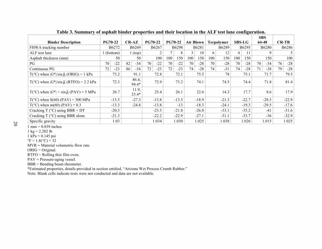
20

Table 3. Summary of asphalt binder properties and their location in the ALF test lane configuration.

Binder Description PG70-22 CR-AZ PG70-22 PG70-22 Air Blown Terpolymer SBS-LG SBS

64-40 CR-TB FHWA tracking number B6272 B6269 B6267 B6298 B6281 B6289 B6295 B6280 B6286 ALF test lane 1 (bottom) 1 (top) 2 7 8 3 10 6 12 4 11 9 5 Asphalt thickness (mm) 50 50 100 100 150 100 150 100 150 100 150 150 100 PG 70 -22 82 -34 70 -22 70 -22 70 -28 70 -28 70 -28 70 -34 76 -28 Continuous PG 72 -23 86 -34 72 -23 72 -23 74 -28 74 -31 74 -28 71 -38 79 -28 T(°C) when |G*|/sin (ORIG) = 1 kPa 73.2 91.1 72.8 72.1 75.5 78 75.1 71.7 79.5

T(°C) when |G*|/sin (RTFO) = 2.2 kPa 72.3 86.4, 94.4* 72.9 73.2 74.1 74.5 74.4 71.8 81.4

T(°C) when |G*| × sin (PAV) = 5 MPa 26.7 11.9, 23.4* 25.4 26.1 22.6 14.3 17.7 8.6 17.9

T(°C) when S(60) (PAV) = 300 MPa -13.5 -27.3 -13.8 -13.5 -18.9 -21.3 -22.7 -28.5 -22.9 T(°C) when m(60) (PAV) = 0.3 -13.3 -24.8 -13.8 -13 -18.3 -24.1 -19.3 -29.5 -17.6 Cracking T (°C) using BBR + DT -20.3 -23.5 -21.8 -26.8 -33.1 -35.2 -41 -31.6 Cracking T (°C) using BBR alone -21.3 -22.2 -22.9 -27.1 -31.1 -33.7 -36 -32.9 Specific gravity 1.03 1.034 1.030 1.025 1.038 1.026 1.015 1.025

1 mm = 0.039 inches 1 kg = 2.202 lb 1 kPa = 0.145 psi °F = 1.8(°C) + 32 MVR = Material volumetric-flow rate. ORIG = Original. RTFO = Rolling thin film oven. PAV = Pressure-aging vessel. BBR = Bending beam rheometer. *Estimated properties, details provided in section entitled, “Arizona Wet Process Crumb Rubber.” Note: Blank cells indicate tests were not conducted and data are not available.

δ δ

δ

21

Figure 15. Graph. High-intermediate-low PG grades of ALF binders in the experiment.

ARIZONA WET PROCESS CRUMB RUBBER MODIFIED ASPHALT

A firm in Phoenix, AZ, developed the blending and modification of the CR-AZ asphalt binder. An unmodified base binder meeting PG58-22 was used along with recycled crumb rubber particles shown in table 4. The blend consisted of 17 percent crumb rubber and 83 percent asphalt binder. Table 5 provides the physical properties of the crumb rubber asphalt binder blend held at 399 °F (204 °C) at various time intervals up to 24 h to evaluate the storage stability of the binder.

Table 4. Recycled crumb rubber particle size in CR-AZ binder.

Sieve Size (mm)

Sieve Number

Percent Passing

Arizona Test Method 714

Gradation Limits(23) 2.36 8 100 100 2.00 10 100 100 1.18 16 98.3 65–100

0.600 30 51.3 20–100 0.300 50 11.9 0–45 0.075 200 0.6 0–5

1 mm = 0.039 inches

22

Table 5. Physical properties of CR-AZ binder during blending.

Test Minutes of Reaction ASTM D6114

Type-I Limits(24) 60 90 240 360 1,440 Viscosity, Haake at 177 °C, cP 2,500 2,900 3,100 3,100 2,900 1,500–4,000 Resilience at 25 °C, percent rebound (ASTM D5329)(25) 36 — 36 — 41 25 minimum Ring and ball softening point, °F (ASTM D36)(26) 147.0 150.0 150.0 149.0 149.0 130 minimum Needle penetration at 4 °C, 200 g, 60 s, 1/10 cm (ASTM D5)(27) 29 — 30 — 31 15 minimum

°F = 1.8(°C) + 32 1 g = 0.035 oz 1 cm = 0.39 inches — Indicates test data were not measured at every point in time.

The size of the crumb rubber particles in the modified asphalt limited the ability to age and test the binder in standard instruments for the PG grading system. The unaged crumb rubber asphalt binder was successfully tested in the DSR, and the temperature at which it met the specification criteria |G*|/sin value of 0.145 psi (1 kPa) at 10 radians/s was 202 °F (94.4 °C). The binder could not be successfully aged in the rolling thin film oven (RTFO) and pressure-aging vessel (PAV) or tested in the DSR for the high-temperature rutting specification criteria |G*|/sin value of 0.32 psi (2.2 kPa) and intermediate-temperature fatigue cracking specification criteria of |G*| × sin value of 725 psi (5,000 kPa).

Research by Shenoy on a variety of binders has shown that RTFO- and PAV-aged PGs can be estimated with some degree of accuracy by relying on the unaged asphalt binder properties.(28,29) The RTFO-aged specification was estimated by adding 11 °F (6 °C) to the temperature at which the original unaged binder met a |G*|/sin value of 0.32 psi (2.2 kPa). The PAV-aged specification was estimated by adding 11 °F (6 °C) to the temperature at which the original unaged binder met a |G*| × sin value of 725 psi (5,000 kPa). The results of the PG grade estimation were a continuous high-temperature grade of 194 °F (90.1 °C) (PG82) and an intermediate-temperature grade of 74 °F (23.4 °C).

The CR-AZ binder was characterized a second time in a more comprehensive manner. The original unaged binder was tested in the DSR using 0.975-inch (25-mm)-diameter plates but with a 0.078-inch (2-mm) gap rather than the standard 0.039-inch (1-mm) gap. The binder did not run out from between the plates and could be trimmed satisfactorily. The original high-temperature PG was 195.98 °F (91.1 °C), which was similar to the 194.18 °F (90.1 °C) PG determined in the earlier characterization. The binder was then aged in an RTFO oven that was tilted backwards to the limit of the specification to prevent the binder from coming out of the bottles. The binder did not completely coat the bottles. The RTFO-aged binder was then characterized in the DSR using 0.975-inch (25-mm)-diameter plates with a 0.078-inch (2-mm) gap. The RTFO high-temperature PG was 187.52 °F (86.4 °C), which was lower than the estimated value discussed above. The binder was then aged in a PAV, degassed, and characterized in a DSR with a 0.312-inch (8-mm)-diameter plate and a 0.078-inch (2-mm) gap as well as a BBR. The intermediate PG was 53.42 °F (11.9 °C), which was lower than the estimated value discussed above. The low temperature PGs from the BBR S-value and m-value were -35.14 and -30.64 °F (-37.3 and -34.8 °C), respectively.

δ

δ

δ

δ

δ

23

MIX DESIGN AND AGGREGATE

The experiment was designed such that the primary variable among the test lanes was binder type, with identical aggregate type and volumetric mix design. The primary mix design of the experiment was based on a standard mixture specified by the Virginia Department of Transportation—a coarse, dense-graded, Superpave®, 0.487-inch (12.5-mm) nominal maximum aggregate gradation. Reclaimed asphalt pavement was excluded from the mix design and experiment to eliminate any influence on the experimental binders. A job-mix formula was submitted to FHWA by the paving contractor for the Superpave® mixture with the unmodified PG70-22 asphalt binder. The optimum asphalt binder content was 5.3 percent by total mass of the mixture based on a 4.0 percent design air-void content at 75 gyrations.

Both coarse and fine aggregate stockpiles were 100 percent crushed stone and did not contain any natural sand. The petrography of the aggregate was a diabase (traprock). To reduce the potential for moisture damage, 1.0 percent hydrated lime was prescribed in all mixtures. Two coarse aggregate stockpiles were used, a No. 78 and No. 68 local designation. Two fine aggregate stockpiles were used, a No. 10 screenings and a grade F and G sand designation. The grade F and G sand was manufactured sand, not natural quartzite sand. The aggregate blending percentages provided by the paving contractor were 16.5 percent No. 68 stockpile, 36.5 percent No. 78 stockpile, 27.0 percent grade F and G sand stockpile, and 20.0 percent No. 10 screenings stockpile.

NCHRP 90-07 research was completed by FHWA and included an evaluation of optimum asphalt content at 75 gyrations at a compaction temperature of 284 °F (140 °C) for a variety of modified asphalts.(20) Modifications included terpolymer, ethylene vinyl acetate, SBS-LG, unmodified PG70-22, SBS radial grafted, and an ethylene styrene interpolymer. The optimum asphalt binder contents at 4.0 percent air void content were 4.4, 4.4, 4.5, 4.6, 4.6, and 4.6 percent, respectively. An air-blown asphalt provided a binder content of 4.8 percent, a chemically modified crumb rubber product provided a binder content of 4.9 percent, and a mixture containing the unmodified PG70-22 asphalt binder with 0.3 percent polyester fiber by aggregate mass provided a significantly higher binder content of 5.4 percent.

In this study, the asphalt binder content was fixed if it provided air voids within a range of 3.5–4.5 percent. The study was designed to evaluate effects of asphalt binder properties on performance. It was expected that there would be a greater tendency to question whether small differences in asphalt binder content confounded the conclusions of the experiment compared to small differences in the design air void level.

Large quantities of coarse and fine aggregate from the paving contractor were delivered to FHWA. The unmodified PG70-22 binder was used to conduct trial compactions. Binder contents of 4.8, 5.3, and 5.8 percent were evaluated. These contents provided air-void levels of 5.9, 5.0, and 3.9 percent, respectively. The hydrated lime to be used in the mixture was added to the fine aggregate stockpile by the paving contractor. The lime and fine aggregate were mixed together in the hot mix drum plant without asphalt. The lime-treated aggregate was then stockpiled. This method of addition resulted in the formation of some lime nuggets. It was hypothesized that the variability in air voids could be the result of inconsistent samples of the lime-treated fine aggregate when batching the aggregates. Compaction tests were performed using samples of the

24

lime-treated No. 10 aggregate taken directly from the stockpile at the hot mix plant to make sure that the Turner-Fairbank Highway Research Center (TFHRC) stockpile was representative of the stockpile at the plant. This mixture also provided air voids of 5.9, 5.0, and 3.9 percent at asphalt binder contents of 4.8, 5.3, and 5.8 percent, respectively. These tests provided no insight concerning the inconsistencies in the air voids and did not rule out the possibility that the dispersion of the hydrated lime was part of the problem.

Construction proceeded with the contractor’s mix design. Volumetric data of the production mixes are shown in table 6. The air-blown, SBS-LG, and SBS 64-40 mixtures fell within the desired air void content range of 3.5–4.5 percent. The CR-TB mixture fell 0.1 percentage points higher than the desired range at 4.6 percent. The 5.0 percent design air void content of the PG70-22 mixture fell outside the desired range by 0.5 percentage points. The fiber mix was evaluated with 0.3 percent fiber by weight of aggregate, and air void contents were outside the desired range at 5.1 percent. Increasing the binder content in laboratory tests created very erratic volumetrics, indicating fibers could be trapping air voids. The weight of the fiber was reduced to 0.2 percent by weight of aggregate, and the air void content was 4.8 percent. The paving contractor needed a tolerance for the amount of polyester fiber to be used, so the allowable range was set at 0.2–0.3 percent by mass of aggregate.

Voids in the mineral aggregate (VMA) of all mixtures met the minimum requirement of 14.0 percent and were greater than 16.0 percent even if the volumetrics of the mixtures were adjusted to a 4.0 percent design air void level. The voids filled with asphalt (VFA) for most of the mixtures met the 65 to 75 percent requirement. The only mixture where the VFA deviated significantly from the requirement was SBS 64-40, which had a VFA of 78 percent. The VMAs and VFAs in table 6 indicate that the aggregate structure provided a high amount of void space, which is rich in asphalt binder.

25

Table 6. Laboratory mix design evaluation of volumetrics.

Asphalt Binder Type PG70-22 CR-AZ Air

Blown SBS- LG CR-TB Terpolymer Fiber

SBS 64-40

Lane 1 (bottom),

2 and 8 1

(top) 3 and

10 4 and

11 5 6 and 12 7 9 Total binder content, percent by mass 5.3 7.1 5.3 5.3 5.3 5.3 5.3 5.3 Effective binder content, percent by mass 5 6.6 5 4.9 5 5 5 4.9 Asphalt binder absorption, percent by mass 0.3 0.5 0.3 0.4 0.3 0.3 0.3 0.4 Effective binder content, percent by total volume 12.5 16 12.6 12.7 12.6 12.5 11.9 12.7 Dust, percent passing the 75- m sieve 6.3 3 6.3 6.3 6.3 6.3 6.3 6.3 Dust to effective binder content 1.26 0.45 1.26 1.29 1.26 1.26 1.26 1.29 Specific gravity of binder 1.03 1.028 1.026 1.023 1.019 1.024 1.03 1.005 Design air voids, percent 5 5.5 4.1 4.2 4.6 4.9 4.8 3.6 VMA at design air voids, percent 17.5 21.5 16.7 16.9 17.3 17.5 18.1 16.3 VFA at design air voids, percent 71.2 74.5 75.4 75.2 73.3 72.1 65.9 78.2 Maximum specific gravity 2.704 2.627 2.703 2.700 2.700 2.701 2.705 2.699 Effective specific gravity of aggregate 2.975 2.981 2.975 2.971 2.974 2.973 2.976 2.981 Bulk dry specific gravity of aggregate 2.947 2.948 2.947 2.947 2.947 2.947 2.934 2.947 1 = 0.039 mil

Gap-Graded Crumb Rubber Mix Design

The CR-AZ mixture was designed according to the Arizona Department of Transportation’s asphalt-rubber asphaltic concrete design specifications.(30) Five materials were used: No. 68 diabase, No. 78 diabase, No. 8P diabase, No. 10 diabase, and hydrated lime. The aggregate blending percentages were 32.7 percent No. 68 stockpile, 46.5 percent No. 78 stockpile, 8.9 percent No. 8P stockpile, and 10.9 percent No. 10 screenings. In addition, 1 percent hydrated lime was used. The 75 blow-per-side Marshall Method was used for the mixture design. The compaction temperature was 325 °F (163 °C). The volumetric requirements were that the air voids had to be between 4.5 and 6.5 percent and the VMA had to be a minimum 19.0 percent. Four asphalt binder contents were tried: 6.0, 7.0, 8.0, and 9.0 percent. The optimum asphalt binder content was found to be 7.1 percent and may appear lower than typical contents near 8 percent for this type of mixture. However, the effective volumetric binder content was 16 percent, and the high specific gravity of the diabase aggregate (2.98) can make gravimetric binder contents appear lower. If the aggregate specific gravity was lower (i.e., around 2.7), then the gravimetric binder content would have been around 7.8 percent.

PAVEMENT TEST FACILITY LAYOUT AND CONSTRUCTION

The FWHA Pavement Test Facility (PTF) and two ALFs are used to rapidly collect data on pavement performance under conditions in which axle loading and pavement temperature are

μ

μm

26

controlled. This facility is also used to study the complex interactions among pavement structures, construction materials, and axle loads. The primary objective of the PTF is to develop and verify new specifications, designs, and test procedures. Previous studies have addressed the relationship of tire pressure to pavement performance, the impact of super-single tires on asphalt pavement performance, the validation of SHRP binder and mixture specifications, and design procedures for ultra-thin white topping concrete overlays. (See references 16–18, 31, and 32.) The two ALF machines can run tests on alternative pavement designs (structures or materials) with fixed loading configurations or, conversely, on identical pavement designs with alternative loading configurations (e.g., by varying tire pressure or axle loading). Each machine is capable of applying an average of 35,000 passes per week with a half-axle load ranging from 7,500 to 19,000 lbf (33 to 84 kN). Each of the PTF’s test lanes is long enough to include two 46- by 14-ft (14- by 4-m) test sections, and each test section can be divided transversely into two test sites. As a result, full paving of the 12 test lanes provides sufficient space for a 48-cell experiment.

The configuration of mixture types in the lanes and layer thickness is shown in figure 16. Each pavement lane is 13 ft (4 m) wide and 160 ft (50 m) long and is divided into four test sites. All pavement lanes consist of an HMA layer and a dense-graded, crushed aggregate base (CAB) course over a uniformly prepared silty clay subgrade categorized as soil classification AASHTO A-4. The total thickness of the HMA and CAB layers is 26 inches (660 mm). Lanes 1 through 7 were constructed with a 4-inch (100-mm)-thick layer of HMA, and lanes 8 through 12 were constructed with a 5.8-inch (150-mm)-thick layer.

1 mm = 0.039 inches

Figure 16. Illustration. Oblique diagram of the test section’s three-dimensional layout.

27

Trenches were cut in past ALF studies and indicate that total rutting was distributed within the asphalt layers and crushed stone layers but did not appear to deform or disturb the subgrade layer, as shown in the example in figure 17. The subgrade was not exposed or disturbed in the construction of the test lanes, but historical data on gradation are available and are summarized in table 7.(33,34) Neither source provides any liquid limits, plastic limits, or plasticity indices or categorizes the subgrade as non-plastic. References 33 and 34 provide additional data, as follows:

• California bearing ratio is reported to be 6.7.

• AASHTO T 99 optimum moisture content and maximum dry densities are reported as 14.9 percent and 111.9 lb/ft3 (1,792 kg/m3), respectively.(35)

• AASHTO T 180 optimum moisture content and maximum dry densities are reported as 11.4 percent and 121.6 lb/ft3 (1,984 kg/m3), respectively.(36)

• The specific gravity of the subgrade was found to be 2.840.

Figure 17. Graph. Pavement layer profile measured from a trench cut in an ALF test

section from past study.(16)

Table 7. Gradation of AASHTO A-4 subgrade. Sieve Size

(mm) Total Percent Passing

Reference 23 Reference 24 25 100 100 14 97 99

12.5 94 — 9.5 92 97

4.75 87 96 2 83 95

0.425 71 85 0.075 34 47

1 mm = 0.039 inches — Indicates test data were not measured for every sieve size.

28

The pavement test lanes were constructed in the summer and fall of 2002. The damaged CAB was removed. The first shaded area beneath the lanes in figure 16 shows where new CAB was placed. The new CAB was tested for gradation, density, moisture content, and surface elevation and met all requirements, as shown in table 8. The CAB was compacted with a vibrating steel wheel roller to a minimum of 156 lb/ft3 (2,529 kg/m3), which was 95 percent of the maximum density. Initially, some of the tests showed that the density was 94 percent of the maximum density, but these sections were reworked so that they met the requirement. The average moisture content was 5.3 percent. Gradation targets of the CAB are given in table 8.

Table 8. CAB gradation.

Sieve Size (mm)

Total Percent Passing

Tolerance (Percent)

Acceptance Range

(Percent) Design/Spec

Range (Percent) 50 100 0 100 100 25 95 5 90–100 94–100

9.5 66 9.5 56.5–75.5 63–72 2 35 7 28–42 32–41

0.425 19 4 15–23 14–24 0.075 8 2 6–10 6–12

1 mm = 0.039 inches

Tanker trucks of the experimental asphalt binders were sent to the paving contractor after coordination and confirmation of the asphalt binder properties with the producers supplying the binder. A blender was delivered to the hot-mix plant for the CR-AZ production, whereas the CR-TB was trucked to the hot mix plant from the terminal. The asphalt mixtures were produced in a counterflow drum plant located in Sterling, VA, 17 mi (27 km) from the PTF site. After transport, trucks unloaded the HMA into a material transfer device (MTD), which fed a rubber tire paver. An infrared camera used during construction verified the MTD was effective in eliminating temperature segregation. An example is shown in figure 18 and figure 19. The numerical image analysis of this particular thermal image taken during October 2002 construction indicates that the temperature of the mix coming out from the back of the paver was about 298–302 °F (148–150 °C) and the coolest parts of the loose mat within view were about 244–248 °F (118–120 °C). All of the test lanes were constructed in two lifts, each 2 or 3 inches (50 or 75 mm) thick, as appropriate. A 13.5-T (12.3-Mg) vibratory roller was used for the breakdown, followed by a 10-T (9.1-Mg) static steel roller for the finish rolling. The upper lift was placed as soon as the lower lift was cool enough to handle the paver, and no tack coat was used between the lifts.

29

Figure 18. Photo. Conventional photo of hot mix placement from the back of the paver.

Figure 19. Photo. Thermal image of hot mix placement from the back of the paver.

A control strip was constructed in the parking lot before each test pavement was placed. This strip was used to determine the appropriate rolling pattern needed to achieve the desired density, to check the calibration of the paving contractor’s nuclear density gauge, and to approve each HMA by determining its asphalt binder content, aggregate gradation, maximum specific gravity, and volumetrics. Density and thickness were checked by sawing rectangular blocks from the pavement. The materials had to meet the specifications before the test pavement could be constructed. These control strips indicated that the target density could be achieved by four to six vibratory passes followed by three to five static passes, depending on the type of mixture. The pavements were compacted within a temperature range of 220–302 °F (105–150 °C).

Specification criteria for the HMA are given in table 9. The paving contractor and FHWA randomly obtained two samples of each plant-produced mixture from the loaded trucks and split them according to AASHTO T 168 and AASHTO T 248.(37,38) The samples were tested for binder content, aggregate gradation, and theoretical maximum specific gravity. The target gradation and limits for the gap-graded CR-AZ mix design and the dense-graded mix design are provided in table 10. Some material was placed and accepted out of specification. The following sections describe the construction data of note for each lane. Air void content taken on cores was

30

measured on the entire core having both lifts. Three cores were taken from the left wheel path, and three cores were taken from the right wheel path. Cores were not split at the lift boundary except for lane 1, where the top lift was the gap-graded CR-AZ mix and the bottom lift was the dense-graded PG70-22 mix. Thickness was measured with two techniques: (1) cores were measured for thickness and (2) the depth of holes drilled to metal survey plates was measured.

Table 9. HMA specifications.

Material Property Test Method Number of Tests Tolerance Aggregate gradation

AASHTO T 30(39) Three per test lane

Target ±3.0 percent for 4.75 mm; target ±2.0 percent for 0.600 mm; target ±0.7 percent for 0.075 mm

Asphalt binder content

AASHTO T 308 ignition oven(40)

Three per test lane

Target ±0.2 percent

AASHTO T 287 nuclear(41)

Three per control strip

No specification

Maximum specific gravity

AASHTO T 209(42) Three per test lane

Target ±0.015

Mixture volumetrics

AASHTO PP28(43) Three per test lane

No specification

In-place density ASTM D2950 nuclear density gauge(44)

15 per lift per test lane

Target ±1 percent

Air voids using cores

AASHTO T 166 and ASTM D3203(45,46)

Six per test lane 7.0 ±1 percent

Thickness using cores

Federal Lands T 501(47) Six per test lane Target ±10 mm

1 mm = 0.039 inches

Table 10. HMA aggregate gradation targets and limits.

Sieve Size Gap-Graded CR-AZ Mix Design, Percent Passing

Dense-Graded 12.5 mm NMAS, Percent Passing

Standard Metric (mm)

Target Blend Limits

Target Blend Limits

1 inch 25 100 100 ¾ inch 19 100 100 ½ inch 12.5 87 94

3/8 inch 9.5 73 85 No. 4 4.75 33 30–36 55 52–58 No. 8 2.36 16 35

No. 16 1.18 11 No. 30 0.6 8 6–10 17 15–19 No. 50 0.3 6 12

No. 100 0.15 5 No. 200 0.075 3 2.3–3.7 6.3 5.6–7.0

NMAS = Nominal maximum aggregate size. Note: Blank cells indicate test data were not measured at sieve size.

31

Quantitative descriptions of each lane’s construction are as follows:

Lane 1, top, CR-AZ: One sample was taken for gradation. Aggregate gradation was within tolerances for the No. 4 (4.75 mm) and No. 30 (0.6 mm) sieves. The No. 200 (0.075 mm) sieve was 0.1 percentage points higher than the tolerance. Only one ignition oven binder content measurement was taken instead of three. The value was 6.7 percent, 0.4 percentage points lower than the target of 7.1 percent. One of three maximum specific gravity measurements was outside the tolerance, resulting in an average outside the tolerance. Two of six cores were outside the air void tolerance, but the average air void content was within the tolerance.

Lane 1, bottom, PG70-22: One sample was taken for gradation. Aggregate gradation was within all three tolerances for the No. 4, No. 30, and No. 200 (4.75, 0.6, and 0.075 mm) sieves. Only one ignition oven binder content measurement was taken instead of three, and it was within the target binder content range. All three maximum specific gravity tests were within tolerance. Two of six cores were outside the air void tolerance, but the average air void content was within tolerance. A total of 4 of 17 drilled holes were outside the thickness tolerance, but the average was within tolerance. Two of six cores were outside the thickness tolerance, but the average was within tolerance.

Lane 2, PG70-22: One sample was taken for gradation data. The aggregate gradation data on the No. 4 (4.75 mm) sieve was 0.8 percentage points lower than tolerance, while the No. 200 (0.075 mm) sieve was 0.2 percentage points lower than tolerance. Only one ignition oven binder content measurement was taken instead of three, and it was within the target binder content range. All three maximum specific gravity tests were within tolerance. Two of six cores were outside the air void tolerance, but the average air void content was within tolerance. A total of 6 of 12 drilled holes indicated thickness outside of tolerance, and average thickness was 0.029 inches (0.75 mm) above tolerance. All six cores and average were within the thickness tolerance.

Lane 3, air blown: Two of three samples were above tolerance on the No. 4 (4.75 mm) sieve, but the average was 1.2 percentage points above tolerance. One of three samples on the No. 30 (0.6 mm) sieve and on the No. 200 (0.075 mm) sieve was above tolerance, but the averages were within tolerance. One of three ignition oven binder content measurements was outside the range, resulting in an average air void content outside the tolerance. One of three maximum specific gravity tests was below tolerance, but the average maximum specific gravity was within tolerance. Four of six cores were outside the air void tolerance, with one high and three low. This resulted in an average air void content below tolerance. Only 1 of 12 drilled holes indicated thickness outside tolerance, and the average was within tolerance. One of the six cores was outside the thickness tolerance, and the average was within tolerance.

Lane 4, SBS-LG: Two gradation samples on the No. 4 (4.75 mm) sieve were outside tolerance. One was above and the other below, but the average was within tolerance. All samples on the No. 30 and No. 200 (0.6 and 0.075 mm) sieves were within tolerance. One of three ignition oven binder content measurements was below tolerance, but the average binder content was within tolerance. All three maximum specific gravity measurements were within tolerance. Three cores were within tolerance and three cores were below tolerance, resulting in an average air void

32

content below tolerance. All 12 drilled holes indicated thickness within tolerance. One of six cores was outside the thickness tolerance, and the average was within tolerance.

Lane 5, CR-TB: All three gradation samples on the No. 4 (4.75 mm) sieve were above tolerance, and the average was 2.1 percentage points above tolerance. All gradation samples on the No. 30 and No. 200 (0.6 and 0.075 mm) sieves were within tolerance. One of three ignition oven asphalt content measurements was above tolerance, and the average was within tolerance. All three maximum specific gravity measurements were within tolerance. Four of six air void cores were outside the air void tolerance, with one high and three low. This resulted in an average air void content within tolerance. Only 3 of 17 drilled holes indicated thickness outside tolerance, but the average was within tolerance. Two of six cores were below the thickness tolerance and resulted in an average thickness 0.052 inches (1.33 mm) below tolerance.

Lane 6, terpolymer: One of three gradation samples on the No. 4 (4.75 mm) sieve was above tolerance, but the average was within tolerance. All gradation samples on the No. 30 and No. 200 (0.6 and 0.075 mm) were within tolerance. Only two measurements were taken for binder content. One of two ignition oven binder content measurements was above tolerance, but the average binder content was within tolerance. Two of three maximum specific gravity tests were taken, and both were within tolerance. Two of six cores were below the air void content tolerance, and the average was within tolerance. A total of 5 of 12 drilled holes were out of the thickness tolerance, but the average was within tolerance. Three of six cores were within the thickness tolerance, and the average was within tolerance.

Lane 7, fiber: All three gradation samples were within tolerance on all sieves. All three ignition oven binder content tests were within tolerance. Corrections were made because fibers were affected by the burn-off oven. All three maximum specific gravity measurements were within tolerance. All six cores taken were within the air void content tolerance. Ten of 32 drilled holes indicated thickness within tolerance. Four of six cores were outside tolerance, and the average was 0.097 inches (2.5 mm) above tolerance.

Lane 8, PG70-22: One of three gradation samples on the No. 4 (4.75 mm) sieve was above tolerance, but the average was within tolerance. All samples on the No. 30 (0.6 mm) sieve were within tolerance. The No. 200 (0.075 mm) sieve had one of three samples below tolerance, but the average was within tolerance. Two of the three binder content measurements were outside tolerance, with one high and one low. The average binder content was within tolerance. All three maximum specific gravity measurements were within the tolerance level. Five of six cores were below the air void tolerance, and the average level was below tolerance. All 12 drilled holes and all six cores were within the thickness tolerance.

Lane 9, SBS-LG: One of three No. 4 (4.75 mm) sieve gradation samples was well below tolerance, resulting in the average being 0.7 percentage points below tolerance. All three gradation samples on the No. 30 (0.6 mm) sieve were within tolerance. All three gradation samples on the No. 200 (0.075 mm) sieve were below tolerance, resulting in an average that was 0.4 percentage points below tolerance. Two of three binder content measurements were outside tolerance, with one high and one low. The average binder content was within tolerance. One of three maximum specific gravity tests was above tolerance, with the average within tolerance. All six cores had air voids lower than tolerance. Three of 12 drilled holes were outside the thickness

33

tolerance, and the average was within tolerance. Five of six cores were below the thickness tolerance, and the average was 0.163 inches (4.17 mm) below tolerance.

Lane 10, air blown: One of three gradation samples on the No. 4 (4.75 mm) sieve was above tolerance, and the average was within tolerance. The No. 30 and No. 200 (0.6 and 0.075 mm) sieves had all samples within tolerance. All three binder content measurements were above tolerance. All three maximum specific gravity tests were within tolerance. One of six cores was within the air void tolerance and contained a mixture of above and below tolerance. The average was below tolerance. Only 1 of 12 drilled holes was outside the thickness tolerance, and the average was within tolerance. One of six cores was outside tolerance, and the average was within tolerance.

Lane 11, SBS-LG: All gradation samples on all sieves were within tolerance. All three binder contents were within tolerance. All three maximum specific gravity measurements were within tolerance. Five of six cores were below tolerance, and the average was below tolerance. A total of 4 of 12 drilled holes were outside the thickness tolerance, and the average was within tolerance. One of six cores was outside the thickness tolerance, and the average was within tolerance.

Lane 12, terpolymer: All three No. 4 (4.75 mm) gradation samples were above tolerance, resulting in an average that was 2.6 percentage points above the tolerance. One of the three No. 30 (0.6 mm) sieve samples and No. 200 (0.075 mm) sieve samples was above tolerance, but the average was within tolerance. All three binder contents were above tolerance. One of three maximum specific gravity measurements was outside tolerance, and the average was within tolerance. Two cores were within tolerance, and four were below tolerance, with the average air void level outside tolerance. All 12 drilled holes and the average were within the thickness tolerance. Two of six cores were outside the thickness tolerance, but the average was within tolerance.

The overall conclusion regarding the construction of the test lanes was that a very tight tolerance was set for the contractor because of the research requirements. The contractor had trouble staying within those tight tolerances for all work. When tolerances were exceeded, the average values lay on or very near the set specification limits. Some construction was rejected. Lanes 4, 7, 8, and 11 were removed and replaced (data not included in this report). Ultimately, lane 7 was reconstructed twice before being accepted. One reconstruction was due entirely to the wrong gradation being delivered. The other lanes that were removed and replaced were due to thickness and density. Practicality had to be balanced with the objective of the experiment. FWD analyses are given chapter 4. Data for the control strips in the parking lot are not included in this report.

Hydrated Lime Distribution

The hydrated lime was added to the No. 10 screenings aggregate by the paving contractor to produce each asphalt mixture. The lime and No. 10 aggregate were mixed together in the hot mix drum plant without asphalt. The lime-treated aggregate was then stockpiled. This method of lime addition resulted in the formation of some lime nuggets, as observed during pavement construction. The lime nuggets are shown in figure 20 and figure 21. The actual lime content distributed in the pavement test lanes was evaluated. Three 6-inch cores were taken from the end

34

and middle of lanes 2 and 3. The cores were drilled with a hammer drill to obtain a sample of dust containing the components of the asphalt mix. Two different drill bits were used to explore the sensitivity of lime content to the size of the dust sample taken. The dust samples were analyzed using the method developed in the TFHRC Chemistry Laboratory.(48) The lime content was calculated assuming that the mix contained 5.3 percent binder.

Figure 20. Photo. Characteristic lime nuggets indicating less than desired uniform mixing.

Figure 21. Photo. Relative size of lime nuggets.

The average lime content for the lane 2 cores was 0.42 percent with a standard deviation of 0.05 percent. The highest value was 0.53 percent, and the lowest was 0.33 percent. The average for dust using the 3/8-inch (9.5-mm) drill was 0.45 percent with a standard deviation of 0.05 percent. The highest value was 0.53 percent, and the lowest was 0.38 percent. The 5/8-inch (16-mm) drill samples gave an average of 0.40 percent lime with a standard deviation of 0.04 percent and values between 0.45 and 0.33 percent.

The results from lane 3 showed one outlier with a lime level of 1.10 percent compared to the average of 0.5 percent. This could be caused by variations in the method. However, since the other results were closer together, it is more likely that the drilling contained a higher lime level, perhaps an undispersed particle. The average for lane 3 was 0.5 percent, with a standard deviation of 0.20 percent. Ignoring the outlier yields an average of 0.45 percent with a standard deviation of 0.06 percent. Ignoring the outlier, the average for dust using the 3/8-inch (9.5-mm) drill was 0.48 percent with a standard deviation of 0.01 percent. The highest value was 0.49 percent, and the lowest was 0.46 percent. The 5/8-inch (16-mm) drill samples gave an average of 0.42 percent, a standard deviation of 0.07 percent, and values between 0.30 and 0.49 percent.

The detailed analysis of lime in lanes 2 and 3 were compared against samples taken from other lanes in table 11. Most tests used hydrochloric acid instead of acetic acid in the procedure, but

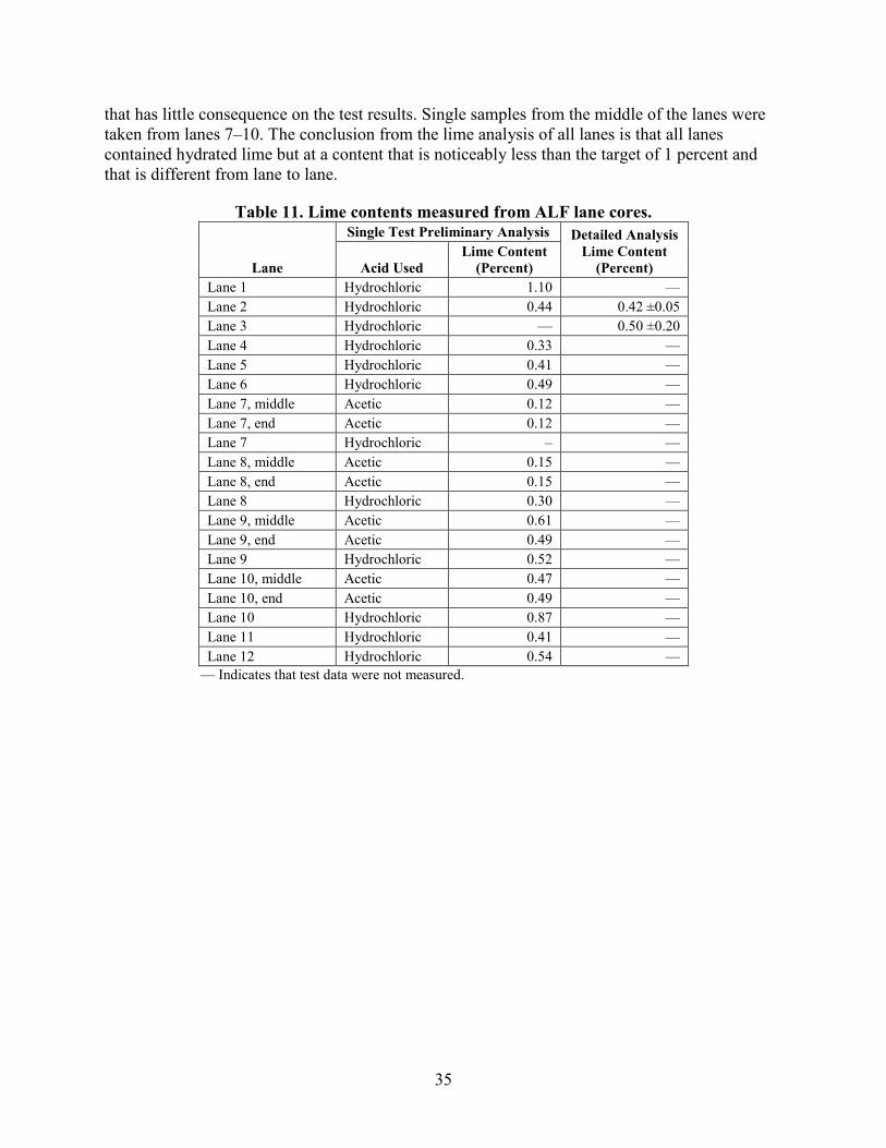
35

that has little consequence on the test results. Single samples from the middle of the lanes were taken from lanes 7–10. The conclusion from the lime analysis of all lanes is that all lanes contained hydrated lime but at a content that is noticeably less than the target of 1 percent and that is different from lane to lane.

Table 11. Lime contents measured from ALF lane cores.

Lane

Single Test Preliminary Analysis Detailed Analysis Lime Content

(Percent) Acid Used Lime Content

(Percent) Lane 1 Hydrochloric 1.10 — Lane 2 Hydrochloric 0.44 0.42 ±0.05 Lane 3 Hydrochloric — 0.50 ±0.20 Lane 4 Hydrochloric 0.33 — Lane 5 Hydrochloric 0.41 — Lane 6 Hydrochloric 0.49 — Lane 7, middle Acetic 0.12 — Lane 7, end Acetic 0.12 — Lane 7 Hydrochloric – — Lane 8, middle Acetic 0.15 — Lane 8, end Acetic 0.15 — Lane 8 Hydrochloric 0.30 — Lane 9, middle Acetic 0.61 — Lane 9, end Acetic 0.49 — Lane 9 Hydrochloric 0.52 — Lane 10, middle Acetic 0.47 — Lane 10, end Acetic 0.49 — Lane 10 Hydrochloric 0.87 — Lane 11 Hydrochloric 0.41 — Lane 12 Hydrochloric 0.54 —

— Indicates that test data were not measured.

37

CHAPTER 3. ALF LOADING CONDITIONS, FULL-SCALE PERFORMANCE, AND ANALYTICAL PLAN

INTRODUCTION

Each ALF test lane can be divided into four quadrants, or sites, as shown in figure 16. FWD testing conducted before placing the asphalt layer and described in subsequent sections indicated variations in unbound layer modulus in sites 1 and 2. General mechanistic-empirical knowledge is that fatigue cracking responses are associated with tensile asphalt strains and can be more influenced by variations in underlying layer properties than can rutting. Therefore, accelerated loading for rutting was conducted in sites 1 and 2, farthest from the parking lot and where the paver began laying the mat. Fatigue loading was conducted in sites 3 and 4, closest to the parking lot, which allowed a longer distance for the paver to place material.

Wheel and Tire Characteristics

Previous FHWA research illustrated that a wide-base 425 type tire, the kind used in this study, induces greater damage than conventional dual tires.(31) The tires used provide a time-saving advantage in accelerated loading. In addition, the simplicity of a single wheel has advantages in primary response mechanistic-empirical analyses. Different tire inflation pressures and wheel loads were used for rutting and fatigue loading. Fatigue loading utilized a 16,000-lbf (71-kN) wheel load and 120-psi (827-kPa) tire inflation pressure. For rutting, the wheel load and tire inflation pressure were 10,000 lbf (44 kN) and 100 psi (689 kPa), respectively.

The imprint of the tire was measured for the 16,000-lbf (71-kN) wheel load and 120-psi (827-kPa) tire inflation pressure condition and is shown in figure 22. The effective contact area was between 110.8 and 117.9 inches2 (0.0715 and 0.0761 m2), which was about 80 to 85 percent of the uniformly loaded circular contact area and resulted in an effective contact stress between 150 and 141 psi (1,032 and 971 kPa).

Figure 22. Illustration. Diagram of 425 tire imprint.

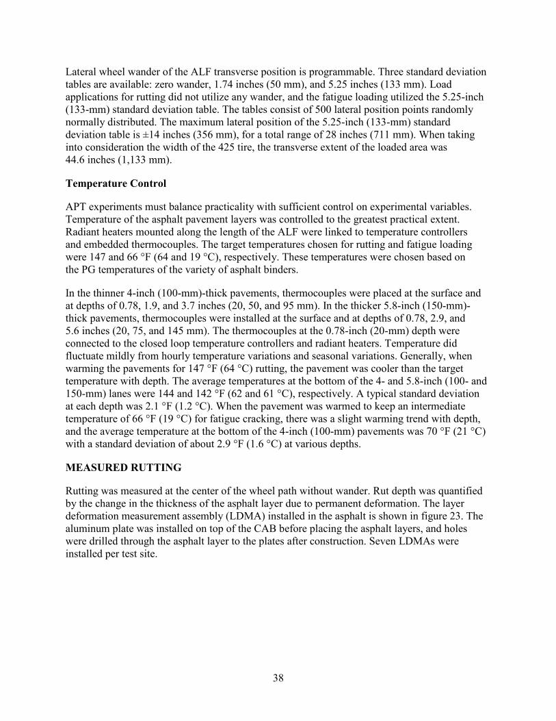
38

Lateral wheel wander of the ALF transverse position is programmable. Three standard deviation tables are available: zero wander, 1.74 inches (50 mm), and 5.25 inches (133 mm). Load applications for rutting did not utilize any wander, and the fatigue loading utilized the 5.25-inch (133-mm) standard deviation table. The tables consist of 500 lateral position points randomly normally distributed. The maximum lateral position of the 5.25-inch (133-mm) standard deviation table is ±14 inches (356 mm), for a total range of 28 inches (711 mm). When taking into consideration the width of the 425 tire, the transverse extent of the loaded area was 44.6 inches (1,133 mm).

Temperature Control

APT experiments must balance practicality with sufficient control on experimental variables. Temperature of the asphalt pavement layers was controlled to the greatest practical extent. Radiant heaters mounted along the length of the ALF were linked to temperature controllers and embedded thermocouples. The target temperatures chosen for rutting and fatigue loading were 147 and 66 °F (64 and 19 °C), respectively. These temperatures were chosen based on the PG temperatures of the variety of asphalt binders.

In the thinner 4-inch (100-mm)-thick pavements, thermocouples were placed at the surface and at depths of 0.78, 1.9, and 3.7 inches (20, 50, and 95 mm). In the thicker 5.8-inch (150-mm)-thick pavements, thermocouples were installed at the surface and at depths of 0.78, 2.9, and 5.6 inches (20, 75, and 145 mm). The thermocouples at the 0.78-inch (20-mm) depth were connected to the closed loop temperature controllers and radiant heaters. Temperature did fluctuate mildly from hourly temperature variations and seasonal variations. Generally, when warming the pavements for 147 °F (64 °C) rutting, the pavement was cooler than the target temperature with depth. The average temperatures at the bottom of the 4- and 5.8-inch (100- and 150-mm) lanes were 144 and 142 °F (62 and 61 °C), respectively. A typical standard deviation at each depth was 2.1 °F (1.2 °C). When the pavement was warmed to keep an intermediate temperature of 66 °F (19 °C) for fatigue cracking, there was a slight warming trend with depth, and the average temperature at the bottom of the 4-inch (100-mm) pavements was 70 °F (21 °C) with a standard deviation of about 2.9 °F (1.6 °C) at various depths.

MEASURED RUTTING

Rutting was measured at the center of the wheel path without wander. Rut depth was quantified by the change in the thickness of the asphalt layer due to permanent deformation. The layer deformation measurement assembly (LDMA) installed in the asphalt is shown in figure 23. The aluminum plate was installed on top of the CAB before placing the asphalt layers, and holes were drilled through the asphalt layer to the plates after construction. Seven LDMAs were installed per test site.

39

Figure 23. Illustration. LDMA used to measure rut depth.

In addition to the LDMA, rod and level surveys were taken on top of the LDMA to quantify total rutting at the surface. The rut depth of the underlying base and subgrade was then calculated as the difference between the total rod-and-level rut depth and the LDMA asphalt rut depth.

Rut depths from the 147 °F (64 °C) tests on the 4-inch (100-mm)-thick lanes are provided in table 12 and figure 24. Rut depths from the 165 °F (74 °C) tests on the 4-inch (100-mm)-thick lanes are provided in table 13 and in figure 25. Rut depths from the 147 °F (64 °C) tests on the 5.8-inch (150-mm)-thick lanes are provided in table 14 and in figure 26. Rut depths from the 113 °F (45 °C) tests on 5.8-inch (150-mm)-thick lanes are provided in table 15 and in figure 27.

Table 12. Rut depths for 4-inch (100-mm) lanes at 147 °F (64 °C). Lane 1,

CR-AZ/PG70-22 Lane 2,

PG70-22 Lane 3,

Air Blown Lane 4, SBS-LG

Lane 5, CR-TB

Lane 6, Terpolymer

Lane 7, Fibers

Passes

Rut Depth (mm) Passes

Rut Depth (mm) Passes

Rut Depth (mm) Passes

Rut Depth (mm) Passes

Rut Depth (mm) Passes

Rut Depth (mm) Passes

Rut Depth (mm)

500 5.83 500 6.27 500 5.36 500 4.88 500 4.66 500 6.62 500 5.23 1,000 6.79 1,000 7.36 1,000 6.66 1,000 5.88 1,000 4.96 1,000 8.01 1,000 6.10 5,000 9.41 2,000 8.71 2,000 7.88 2,000 6.53 2,000 5.75 2,000 9.41 2,000 6.79 10,000 10.28 5,000 9.54 4,100 9.27 3,000 7.23 5,000 6.49 5,000 11.36 5,000 8.49 25,000 11.63 10,000 10.54 10,000 10.49 5,000 8.49 10,000 7.84 10,000 14.24 10,000 9.36 50,000 13.02 25,000 12.19 15,000 11.06 10,000 9.84 25,000 8.36 15,000 14.76 25,000 10.54 53,100 13.02 50,000 13.72 20,000 11.93 25,000 10.93 50,000 9.06 20,000 15.50 50,000 11.02

— — — — 25,000 12.58 35,000 11.67 — — 25,000 15.99* 75,000 11.63 — — — — 30,000 12.89 50,000 12.80 — — — — 100,000 11.84 — — — — — — — — — — — — 125,000 12.50

1 mm = 0.039 inches — Indicates test data were not taken because loading had ended. * Extrapolated.

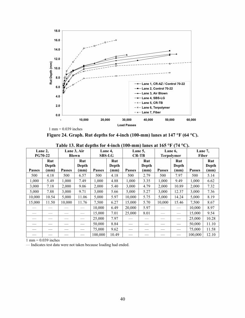
40

1 mm = 0.039 inches

Figure 24. Graph. Rut depths for 4-inch (100-mm) lanes at 147 °F (64 °C).

Table 13. Rut depths for 4-inch (100-mm) lanes at 165 °F (74 °C). Lane 2,

PG70-22 Lane 3, Air

Blown Lane 4, SBS-LG

Lane 5, CR-TB

Lane 6, Terpolymer

Lane 7, Fiber

Passes

Rut Depth (mm) Passes

Rut Depth (mm) Passes

Rut Depth (mm) Passes

Rut Depth (mm) Passes

Rut Depth (mm) Passes

Rut Depth (mm)

500 4.18 500 6.57 500 4.18 500 2.79 500 7.97 500 5.14 1,000 5.49 1,000 7.49 1,000 4.88 1,000 3.35 1,000 9.49 1,000 6.62 3,000 7.18 2,000 9.06 2,000 5.40 3,000 4.79 2,000 10.89 2,000 7.32 5,000 7.88 3,000 9.71 3,000 5.66 5,000 5.27 3,000 12.37 3,000 7.36

10,000 10.54 5,000 11.06 5,000 5.97 10,000 5.75 5,000 14.24 5,000 8.19 15,000 11.50 10,000 11.76 7,500 6.27 15,000 5.70 10,000 15.46 7,500 8.67

— — — — 10,000 6.49 20,000 5.97 — — 10,000 8.97 — — — — 15,000 7.01 25,000 8.01 — — 15,000 9.54 — — — — 25,000 7.97 — — — — 25,000 10.28 — — — — 50,000 8.84 — — — — 50,000 11.10 — — — — 75,000 9.62 — — — — 75,000 11.58 — — — — 100,000 10.49 — — — — 100,000 12.10

1 mm = 0.039 inches — Indicates test data were not taken because loading had ended.

0.0

2.0

4.0

6.0

8.0

10.0

12.0

14.0

16.0

18.0

- 10,000 20,000 30,000 40,000 50,000 60,000

Load Passes

Rut

Dep

th (m

m)

Lane 1, CR-AZ / Control 70-22Lane 2, Control 70-22Lane 3, Air BlownLane 4, SBS-LGLane 5, CR-TBLane 6, TerpolymerLane 7, Fiber

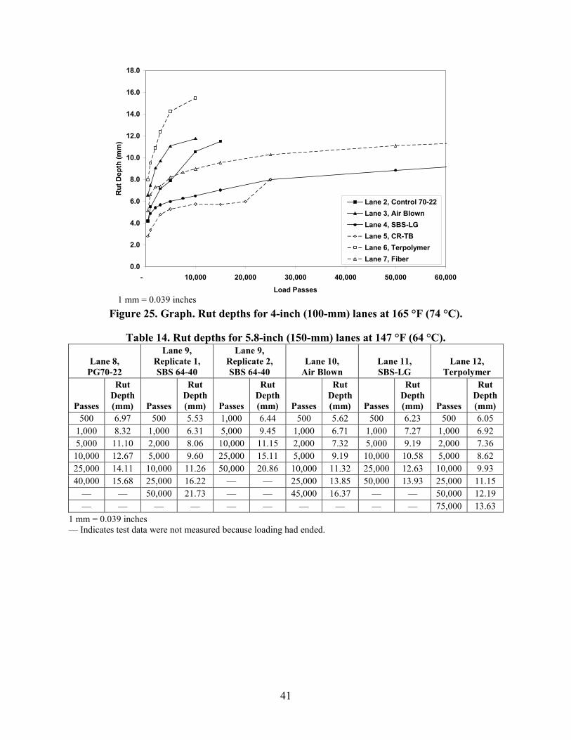
41

1 mm = 0.039 inches

Figure 25. Graph. Rut depths for 4-inch (100-mm) lanes at 165 °F (74 °C).

Table 14. Rut depths for 5.8-inch (150-mm) lanes at 147 °F (64 °C).

Lane 8, PG70-22

Lane 9, Replicate 1, SBS 64-40

Lane 9, Replicate 2, SBS 64-40

Lane 10, Air Blown

Lane 11, SBS-LG

Lane 12, Terpolymer

Passes

Rut Depth (mm) Passes

Rut Depth (mm) Passes

Rut Depth (mm) Passes

Rut Depth (mm) Passes

Rut Depth (mm) Passes

Rut Depth (mm)

500 6.97 500 5.53 1,000 6.44 500 5.62 500 6.23 500 6.05 1,000 8.32 1,000 6.31 5,000 9.45 1,000 6.71 1,000 7.27 1,000 6.92 5,000 11.10 2,000 8.06 10,000 11.15 2,000 7.32 5,000 9.19 2,000 7.36 10,000 12.67 5,000 9.60 25,000 15.11 5,000 9.19 10,000 10.58 5,000 8.62 25,000 14.11 10,000 11.26 50,000 20.86 10,000 11.32 25,000 12.63 10,000 9.93 40,000 15.68 25,000 16.22 — — 25,000 13.85 50,000 13.93 25,000 11.15

— — 50,000 21.73 — — 45,000 16.37 — — 50,000 12.19 — — — — — — — — — — 75,000 13.63

1 mm = 0.039 inches — Indicates test data were not measured because loading had ended.

0.0

2.0

4.0

6.0

8.0

10.0

12.0

14.0

16.0

18.0

- 10,000 20,000 30,000 40,000 50,000 60,000

Load Passes

Rut

Dep

th (m

m)

Lane 2, Control 70-22Lane 3, Air BlownLane 4, SBS-LGLane 5, CR-TBLane 6, TerpolymerLane 7, Fiber

42

1 mm = 0.039 inches

Figure 26. Graph. Rut depths for 5.8-inch (150-mm) lanes at 147 °F (64 °C).

Table 15. Rut depths for 5.8-inch (150-mm) lanes at 113 °F (45 °C). Lane 8, PG70-22 Lane 10, Air Blown Lane 11, SBS-LG

Passes Rut Depth

(mm) Passes Rut Depth

(mm) Passes Rut Depth

(mm) 500 2.39 1,000 1.79 500 2.44

1,000 3.44 5,000 3.05 1,000 2.70 5,000 4.83 10,000 3.79 5,000 3.74

10,000 4.53 25,000 5.01 10,000 4.31 25,000 5.18 50,000 5.88 25,000 4.53 50,000 5.57 75,000 6.27 50,000 4.83 75,000 5.62 108,000 7.18 75,000 4.96

100,000 6.27 125,000 7.53 100,000 5.05 132,250 6.84 149,200 7.84 125,000 5.05 150,000 7.18 175,000 8.10 150,000 5.36 175,000 7.36 200,000 8.45 175,000 5.36 200,000 7.58 225,000 8.71 200,000 5.70 225,000 7.97 250,000 8.84 235,000 5.79

— — 275,000 9.01 250,000 6.01 — — 300,000 9.27 275,000 6.18 — — — — 300,000 6.14

1 mm = 0.039 inches — Indicates test data were not measured because loading had ended.

0.00

5.00

10.00

15.00

20.00

25.00

- 10,000 20,000 30,000 40,000 50,000 60,000 70,000 80,000

Load Passes

Rut

Dep

th (m

m)

Lane 8, Control 70-22Lane 9, SBS 64-40 (1)Lane 9, SBS 64-40 (2)Lane 10, Air BlownLane 11, SBS-LGLane 12, Terpolymer

43

1 mm = 0.039 inches

Figure 27. Graph. Rut depths for 5.8-inch (150-mm) lanes at 113 °F (45 °C).

The 147 °F (64 °C) rut tests were the primary rut tests in both thicknesses. The tests began between June and December 2003 and ended between June 2003 and January 2004, except for the first replicate of lane 9 SBS 64-40, which was tested in November 2002. A statistical f-test and t-test based on the average and standard deviation of rutting between the two replicate tests in lane 9 SBS 64-40 indicated the construction provided statistically equivalent rutting. The rutting performance of all lanes was ranked at 25,000 passes for the primary 147 °F (64 °C) tests with the standard deviation from the seven points of measure, as shown in table 16 and figure 28. Statistical f-tests and t-tests at 95 percent significance were conducted, and the results in table 17 indicate that all lanes provided the same performance statistically except the CR-TB section in lane 5, which was only similar to the fiber section in lane 7. The terpolymer section in lane 6 had similarities with its next two closest ranked sections, air blown in lane 3 and PG70-22 in lane 2.

Table 16. Ranked rut depth of 4-inch (100-mm) lanes at 147 °F (64 °C) and 25,000 passes.

Lane Average Rut Depth (mm)

Standard Deviation Rut Depth (mm)

Lane 5, CR-TB 8.4 0.72 Lane 7, fiber 10.5 1.67 Lane 4, SBS-LG 10.9 0.78 Lane 1, CR-AZ/ PG70-22 11.6 1.47

Lane 2, PG70-22 12.2 1.79 Lane 3, air blown 12.6 1.76 Lane 6, terpolymer 16.0 3.19

1 mm = 0.039 inches

0.00

1.00

2.00

3.00

4.00

5.00

6.00

7.00

8.00

9.00

10.00

- 50,000 100,000 150,000 200,000 250,000 300,000 350,000

Load Passes

Rut

Dep

th (m

m)

Lane 8, Control 70-22Lane 10, Air BlownLane 11, SBS-LG

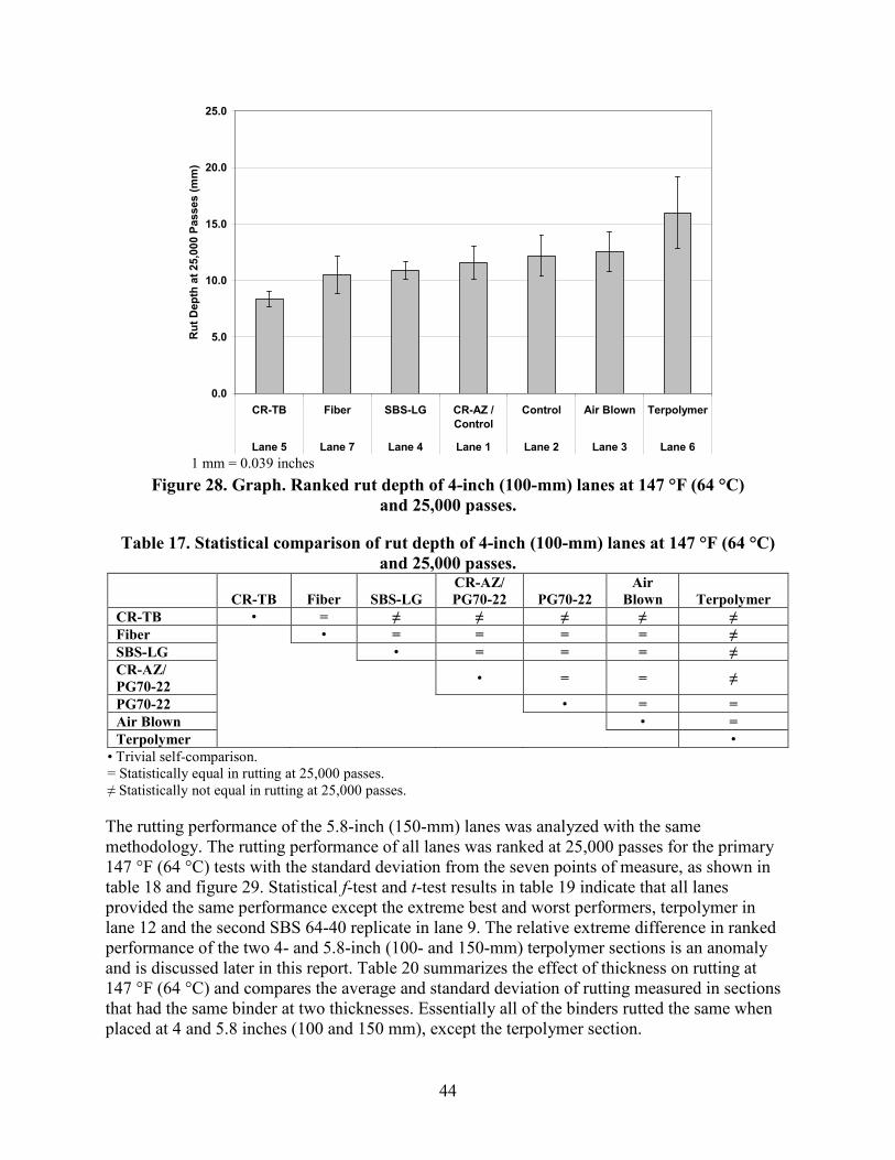
44

1 mm = 0.039 inches

Figure 28. Graph. Ranked rut depth of 4-inch (100-mm) lanes at 147 °F (64 °C) and 25,000 passes.

Table 17. Statistical comparison of rut depth of 4-inch (100-mm) lanes at 147 °F (64 °C) and 25,000 passes.

CR-TB Fiber SBS-LG CR-AZ/ PG70-22 PG70-22

Air Blown Terpolymer

CR-TB • = ≠ ≠ ≠ ≠ ≠ Fiber • = = = = ≠ SBS-LG • = = = ≠ CR-AZ/ PG70-22 • = = ≠

PG70-22 • = = Air Blown • = Terpolymer •

• Trivial self-comparison. = Statistically equal in rutting at 25,000 passes. ≠ Statistically not equal in rutting at 25,000 passes.

The rutting performance of the 5.8-inch (150-mm) lanes was analyzed with the same methodology. The rutting performance of all lanes was ranked at 25,000 passes for the primary 147 °F (64 °C) tests with the standard deviation from the seven points of measure, as shown in table 18 and figure 29. Statistical f-test and t-test results in table 19 indicate that all lanes provided the same performance except the extreme best and worst performers, terpolymer in lane 12 and the second SBS 64-40 replicate in lane 9. The relative extreme difference in ranked performance of the two 4- and 5.8-inch (100- and 150-mm) terpolymer sections is an anomaly and is discussed later in this report. Table 20 summarizes the effect of thickness on rutting at 147 °F (64 °C) and compares the average and standard deviation of rutting measured in sections that had the same binder at two thicknesses. Essentially all of the binders rutted the same when placed at 4 and 5.8 inches (100 and 150 mm), except the terpolymer section.

0.0

5.0

10.0

15.0

20.0

25.0

CR-TB Fiber SBS-LG CR-AZ /Control

Control Air Blown Terpolymer

Lane 5 Lane 7 Lane 4 Lane 1 Lane 2 Lane 3 Lane 6

Rut

Dep

th a

t 25,

000

Pass

es (m

m)

45

Table 18. Ranked rut depth of 5.8-inch (150-mm) lanes at 147 °F (64 °C) and 25,000 passes.

Lane Average Rut Depth (mm)

Standard Deviation Rut Depth (mm)

Lane 12, terpolymer 11.1 2.79 Lane 11, SBS-LG 12.6 1.23 Lane 10, air blown 13.8 2.29 Lane 8, PG70-22 14.1 2.14

Lane 9 SBS 64-40 (1) 15.1 3.84 SBS 64-40 (2) 17.3 8.00

1 mm = 0.039 inches

1 mm = 0.039 inches

Figure 29. Graph. Ranked rut depth of 5.8-inch (150-mm) lanes at 147 °F (64 °C) and 25,000 passes.

Table 19. Statistical comparison of rut depth of 5.8-inch (150-mm) lanes at 147 °F (64 °C) and 25,000 passes.

Terpolymer SBS-LG Air Blown PG70-22 SBS

64-40 (1) SBS

64-40 (2) Terpolymer • = = = = ≠ SBS-LG • = = = = Air Blown • = = = PG70-22 • = = SBS 64-40 (1) • = SBS 64-40 (2) •

• Trivial self-comparison. = Statistically equal in rutting at 25,000 passes. ≠ Statistically not equal in rutting at 25,000 passes.

0.0

5.0

10.0

15.0

20.0

25.0

30.0

Terpolymer SBS-LG Air Blown Control SBS 64-40 (1) SBS 64-40 (2)

Lane 12 Lane 11 Lane 10 Lane 8 Lane 9

Rut

Dep

th a

t 25,

000

Pass

es (m

m)

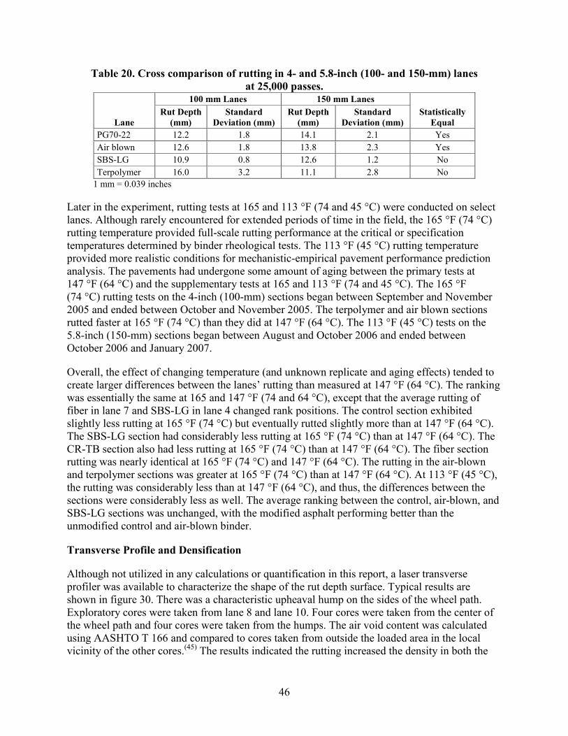
46

Table 20. Cross comparison of rutting in 4- and 5.8-inch (100- and 150-mm) lanes at 25,000 passes.

Lane

100 mm Lanes 150 mm Lanes Statistically

Equal Rut Depth

(mm) Standard

Deviation (mm) Rut Depth

(mm) Standard

Deviation (mm) PG70-22 12.2 1.8 14.1 2.1 Yes Air blown 12.6 1.8 13.8 2.3 Yes SBS-LG 10.9 0.8 12.6 1.2 No Terpolymer 16.0 3.2 11.1 2.8 No

1 mm = 0.039 inches

Later in the experiment, rutting tests at 165 and 113 °F (74 and 45 °C) were conducted on select lanes. Although rarely encountered for extended periods of time in the field, the 165 °F (74 °C) rutting temperature provided full-scale rutting performance at the critical or specification temperatures determined by binder rheological tests. The 113 °F (45 °C) rutting temperature provided more realistic conditions for mechanistic-empirical pavement performance prediction analysis. The pavements had undergone some amount of aging between the primary tests at 147 °F (64 °C) and the supplementary tests at 165 and 113 °F (74 and 45 °C). The 165 °F (74 °C) rutting tests on the 4-inch (100-mm) sections began between September and November 2005 and ended between October and November 2005. The terpolymer and air blown sections rutted faster at 165 °F (74 °C) than they did at 147 °F (64 °C). The 113 °F (45 °C) tests on the 5.8-inch (150-mm) sections began between August and October 2006 and ended between October 2006 and January 2007.

Overall, the effect of changing temperature (and unknown replicate and aging effects) tended to create larger differences between the lanes’ rutting than measured at 147 °F (64 °C). The ranking was essentially the same at 165 and 147 °F (74 and 64 °C), except that the average rutting of fiber in lane 7 and SBS-LG in lane 4 changed rank positions. The control section exhibited slightly less rutting at 165 °F (74 °C) but eventually rutted slightly more than at 147 °F (64 °C). The SBS-LG section had considerably less rutting at 165 °F (74 °C) than at 147 °F (64 °C). The CR-TB section also had less rutting at 165 °F (74 °C) than at 147 °F (64 °C). The fiber section rutting was nearly identical at 165 °F (74 °C) and 147 °F (64 °C). The rutting in the air-blown and terpolymer sections was greater at 165 °F (74 °C) than at 147 °F (64 °C). At 113 °F (45 °C), the rutting was considerably less than at 147 °F (64 °C), and thus, the differences between the sections were considerably less as well. The average ranking between the control, air-blown, and SBS-LG sections was unchanged, with the modified asphalt performing better than the unmodified control and air-blown binder.

Transverse Profile and Densification

Although not utilized in any calculations or quantification in this report, a laser transverse profiler was available to characterize the shape of the rut depth surface. Typical results are shown in figure 30. There was a characteristic upheaval hump on the sides of the wheel path. Exploratory cores were taken from lane 8 and lane 10. Four cores were taken from the center of the wheel path and four cores were taken from the humps. The air void content was calculated using AASHTO T 166 and compared to cores taken from outside the loaded area in the local vicinity of the other cores.(45) The results indicated the rutting increased the density in both the

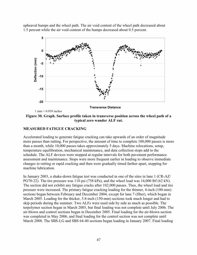
47

upheaval humps and the wheel path. The air void content of the wheel path decreased about 1.5 percent while the air void content of the humps decreased about 0.5 percent.

1 mm = 0.039 inches

Figure 30. Graph. Surface profile taken in transverse position across the wheel path of a typical zero wander ALF rut.

MEASURED FATIGUE CRACKING

Accelerated loading to generate fatigue cracking can take upwards of an order of magnitude more passes than rutting. For perspective, the amount of time to complete 100,000 passes is more than a month, while 10,000 passes takes approximately 5 days. Machine relocations, setup, temperature equilibration, mechanical maintenance, and data collection stops add to the schedule. The ALF devices were stopped at regular intervals for both pavement performance assessment and maintenance. Stops were more frequent earlier in loading to observe immediate changes in rutting or rapid cracking and then were gradually timed farther apart, stopping for machine lubrication.

In January 2003, a shake-down fatigue test was conducted in one of the sites in lane 1 (CR-AZ/ PG70-22). The tire pressure was 110 psi (758 kPa), and the wheel load was 14,000 lbf (62 kN). The section did not exhibit any fatigue cracks after 102,000 passes. Thus, the wheel load and tire pressure were increased. The primary fatigue cracking loading for the thinner, 4-inch (100-mm) sections began between February and December 2004, except for lane 7 (fiber), which began in March 2005. Loading for the thicker, 5.8-inch (150-mm) sections took much longer and had to skip periods during the summer. Two ALFs were used side by side as much as possible. The terpolymer section began in March 2005, but final loading was not complete until July 2006. The air-blown and control sections began in December 2005. Final loading for the air-blown section was completed in May 2006, and final loading for the control section was not complete until March 2008. The SBS-LG and SBS 64-40 sections began loading in January 2007. Final loading

-20

-15

-10

-5

0

5

Transverse Distance

Def

lect

ion

(mm

)

48

for the SBS-LG section was not complete until June 2008, and loading of the SBS 64-40 section ended in July 2007.

Photographs of typical cracked surfaces are shown in figure 31. Cracks were manually traced onto clear Mylar® plastic sheets as they formed at the surface of the pavements. Different color pens were used to correspond to the number of load repetitions. Two approaches were used to process the data. One was to measure the total crack length, and the other was to measure the percentage of area cracked in the loaded area, about 3.4 ft (1 m) wide and 33 ft (10 m) long. A cracked area was considered when individual cracks had grown and met each other, forming a network of cracks. The loaded area was divided into 1- by 1-ft (30- by 30-cm) units to quantify the percent cracked area.

Figure 31. Photo. Typical cracking pattern in loaded ALF wheel paths.

An analysis by Qi et al. found that fatigue cracks begin as small longitudinal cracks.(49) A simplified classification criteria was used to categorize cracks as longitudinal or transverse using a 45-degree orientation line. Cracks began as longitudinal, and as distributed cracking increased, the orientation became less longitudinal. For example, the ratio of longitudinal to transverse cracks for early loading was as high as 9, but after a significant amount of cracking had occurred toward the end of loading, the ratio was typically around 3. The apparent dominance of longitudinal cracks could be because a single tire was used instead of a dual tire and also because the transverse strain at the bottom of the asphalt layer was tensile while the longitudinal strain transitions from compression to tension and then back to tension as the wheel passes. Repeated tensile-only transverse strains causing longitudinal cracking could be more damaging than any healing from mixed tensile and compressive strains in the other orientation.

Fatigue cracking results at 66 °F (19 °C) for the 4-inch (100-mm) lanes are shown in table 21 and table 22 and graphically in figure 32 and figure 33. Fatigue cracking results at 66 °F (19 °C) for the 5.8-inch (150-mm) lanes are shown in table 23 and table 24 and graphically in figure 34 and figure 35.

Table 21. Cumulative crack length in 4-inch (100-mm) fatigue crack sections. Lane 1,

CR-AZ/PG70-22 Lane 2,

PG70-22 Lane 3,

Air Blown Lane 4, SBS-LG

Lane 5, CR-TB

Lane 6, Terpolymer

Lane 7, Fiber

Passes

Crack Length

(m) Passes

Crack Length

(m) Passes

Crack Length

(m) Passes

Crack Length

(m) Passes

Crack Length

(m) Passes

Crack Length

(m) Passes

Crack Length

(m) 0 0.0 25,000 0.0 5,000 0.0 125,000 0.0 25,000 0.0 75,000 0.0 200,000 0.0

125,000 0.0 35,000 14.3 10,000 0.8 150,000 2.0 26,000 0.1 100,000 9.2 225,000 4.0 150,000 0.0 50,000 31.5 25,000 13.6 175,000 9.0 35,000 1.5 125,000 13.7 250,000 8.0 175,000 0.0 75,000 56.5 50,000 52.5 200,000 21.5 50,000 2.0 150,000 33.1 275,000 9.0 201,000 0.0 92,100 81.4 75,000 86.5 225,000 32.0 65,000 11.3 175,000 50.0 300,000 15.2 225,000 0.0 100,000 90.6 93,500 108.6 250,000 39.5 75,000 13.6 200,000 66.3 — — 250,000 0.0 — — — — 275,000 56.1 100,000 24.9 — — — — 275,000 0.0 — — — — 300,000 59.8 — — — — — — 375,000 0.0 — — — — — — — — — — — —

1 m = 3.28 ft — Indicates test data were not measured because loading had ended.

Table 22. Percent cracked area in 4-inch (100-mm) fatigue crack sections. Lane 1,

CR-AZ/PG70-22 Lane 2,

PG70-22 Lane 3,

Air Blown Lane 4, SBS-LG

Lane 5, CR-TB

Lane 6, Terpolymer Lane 7, Fiber

Passes

Percent Cracked

Area Passes

Percent Cracked

Area Passes

Percent Cracked

Area Passes

Percent Cracked

Area Passes

Percent Cracked

Area Passes

Percent Cracked

Area Passes

Percent Cracked

Area 0 0.0 25,000 0.0 5,000 0.0 125,000 0.0 25,000 0.0 75,000 0.0 200,000 0.0

125,000 0.0 35,000 17.7 10,000 1.0 150,000 1.1 26,000 0.0 100,000 12.5 225,000 7.3 150,000 0.0 50,000 38.5 25,000 15.6 175,000 7.3 35,000 1.0 125,000 14.6 250,000 9.4 175,000 0.0 75,000 65.6 50,000 42.7 200,000 20.8 50,000 2.1 150,000 30.2 275,000 10.4 201,000 0.0 92,100 90.6 75,000 69.8 225,000 31.3 65,000 16.7 175,000 43.8 300,000 14.6 225,000 0.0 100,000 100.0 93,500 78.1 250,000 37.5 75,000 18.8 200,000 59.4 — — 250,000 0.0 — — — — 275,000 54.2 100,000 41.7 — — — — 275,000 0.0 — — — — 300,000 57.3 — — — — — — 375,000 0.0 — — — — — — — — — — — —

—Indicates test data were not measured because loading had ended.

49

50

1 m = 3.28 ft

Figure 32. Graph. Cumulative crack length versus ALF passes in 4-inch (100-mm) 66 °F (19 °C) fatigue loaded sections.

Figure 33. Graph. Percent cracked area versus ALF passes in 4-inch (100-mm)

66 °F (19 °C) fatigue loaded sections.

0.0

20.0

40.0

60.0

80.0

100.0

120.0

- 50,000 100,000 150,000 200,000 250,000 300,000 350,000 400,000

Cum

ulat

ive

Cra

ck L

engt

h (m

)

Load Passes

Lane 1, CR-AZ / Control

Lane 2, Control

Lane 3, Air Blown

Lane 4, SBS-LG

Lane 5, CR-TB

Lane 6, Terpolymer

Lane 7, Fiber

0.0

20.0

40.0

60.0

80.0

100.0

120.0

- 50,000 100,000 150,000 200,000 250,000 300,000 350,000 400,000

% C

rack

ed A

rea

Load Passes

Lane 1, CR-AZ / Control

Lane 2, Control

Lane 3, Air Blown

Lane 4, SBS-LG

Lane 5, CR-TB

Lane 6, Terpolymer

Lane 7, Fiber

51

Table 23. Cumulative crack length in 5.8-inch (150-mm) fatigue crack sections. Lane 8,

PG70-22 Lane 9,

SBS 64-40 Lane 10,

Air Blown Lane 11, SBS-LG

Lane 12, Terpolymer

Passes

Crack Length

(m) Passes

Crack Length

(m) Passes

Crack Length

(m) Passes

Crack Length

(m) Passes

Crack Length

(m) 300,000 0.00 150,000 0.00 75,000 0.00 50,000 0.00 225,000 0.00 325,000 1.00 250,000 0.00 100,000 0.25 125,000 0.00 275,000 0.00 425,000 3.00 340,000 0.00 125,000 7.49 200,000 0.00 400,000 0.00

— — 350,000 1.93 160,000 12.42 310,000 0.00 — — — — 400,000 4.88 175,000 17.75 673,000 0.00 — — — — 425,000 6.71 200,000 25.81 — — — — — — — — 250,000 32.18 — — — — — — — — 275,000 36.02 — — — — — — — — 300,000 41.78 — — — — — — — — 325,000 46.05 — — — — — — — — 350,000 50.37 — — — — — — — — 375,000 52.83 — — — —

1 m = 3.28 ft — Indicates test data were not measured because loading had ended.

Table 24. Percent cracked area in 5.8- inch (150-mm) fatigue crack sections. Lane 8

PG70-22 Lane 9

SBS 64-40 Lane 10

Air Blown Lane 11 SBS-LG

Lane 12 Terpolymer

Passes

Percent Cracked

Area Passes

Percent Cracked

Area Passes

Percent Cracked

Area Passes

Percent Cracked

Area Passes

Percent Cracked

Area 300,000 0.00 150,000 0.00 100,000 0.00 50,000 0.00 225,000 0.00 325,000 1.04 250,000 0.00 125,000 10.42 125,000 0.00 275,000 0.00 425,000 3.13 340,000 0.00 160,000 11.46 200,000 0.00 400,000 0.00

— — 350,000 1.04 175,000 15.63 673,000 0.00 — — — — 400,000 9.38 200,000 27.08 — — — — — — 425,000 11.46 250,000 34.38 — — — — — — — — 275,000 35.42 — — — — — — — — 300,000 37.50 — — — — — — — — 325,000 39.58 — — — — — — — — 350,000 45.83 — — — — — — — — 375,000 50.00 — — — —

— Test data were not measured because loading had ended.

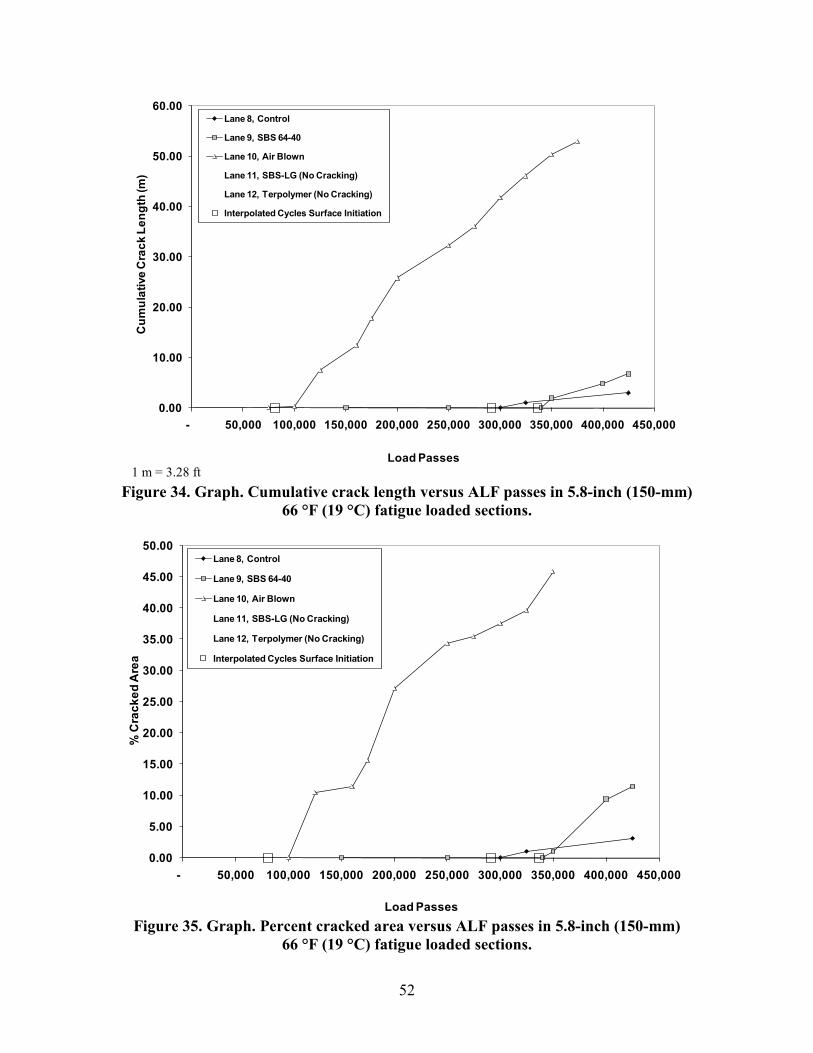
52

1 m = 3.28 ft

Figure 34. Graph. Cumulative crack length versus ALF passes in 5.8-inch (150-mm) 66 °F (19 °C) fatigue loaded sections.

Figure 35. Graph. Percent cracked area versus ALF passes in 5.8-inch (150-mm)

66 °F (19 °C) fatigue loaded sections.

0.00

10.00

20.00

30.00

40.00

50.00

60.00

- 50,000 100,000 150,000 200,000 250,000 300,000 350,000 400,000 450,000

Cum

ulat

ive

Cra

ck L

engt

h (m

)

Load Passes

Lane 8, Control

Lane 9, SBS 64-40

Lane 10, Air Blown

Lane 11, SBS-LG (No Cracking)

Lane 12, Terpolymer (No Cracking)

Interpolated Cycles Surface Initiation

0.00

5.00

10.00

15.00

20.00

25.00

30.00

35.00

40.00

45.00

50.00

- 50,000 100,000 150,000 200,000 250,000 300,000 350,000 400,000 450,000

% C

rack

ed A

rea

Load Passes

Lane 8, Control

Lane 9, SBS 64-40

Lane 10, Air Blown

Lane 11, SBS-LG (No Cracking)

Lane 12, Terpolymer (No Cracking)

Interpolated Cycles Surface Initiation

53

Unlike the rutting performance, there was a more separated variation in the fatigue cracking performance. There is a nearly identical quantitative relationship between the two measures of fatigue cracking; both quantify and rank the performance of the different sections the same. Sections that exhibited surface cracks sooner also developed cracks faster. No cracking was observed for the composite pavement in lane 1 with gap-graded CR-AZ above the dense-graded PG70-22 mixture. Lane 7 (fiber) was very resistant to fatigue cracking and had the least cracking of all the 4-inch (100-mm) sections exhibiting fatigue cracks at the surface. Overall, less cracking and more load passes were required to achieve fatigue crack initiation in the 5.8-inch (150 mm) sections than in the thinner 4-inch (100-mm) sections. Lane 10, with air blown binder, exhibited the largest amount of cracking, as it did in the 4-inch (100-mm) section. The fatigue cracking response of the SBS 64-40 and the PG70-22 binder were intermixed. The lane 8 PG70-22 section had a lower fatigue cracking response curve but achieved surface cracks sooner than lane 9 with SBS 64-40. Cores taken from the PG70-22 section to exhume strain gauges showed delamination at the lift boundary, as shown in figure 36. Lane 11 (SBS-LG) and lane 12 (terpolymer) did not exhibit any surface crack initiation. Cores were also taken from lanes 11 and 12 to look for subsurface bottom-up fatigue cracking that may have initiated but did not propagate through. None of the cores from either lane 11 or 12 indicated that cracking had begun. Some delamination was observed in the cores from lane 11 but less than the cores from lane 8.

Figure 36. Photo. Cores from lane 8 (PG70-22).

The slope of cracking with passes is plotted against the number of cycles to surface crack initiation in figure 37, which shows two different relationships depending on the thickness of the asphalt. The relationship for the thinner, 4-inch (100-mm) lanes has more points and is better defined than the three points from the thicker, 5.8-inch (150-mm) lanes. In order to build a complete set of rankings for all lanes, extrapolations of this relationship were used to estimate the number of cycles to a 25 percent cracked area and 82 ft (25 m) of cumulative crack length for lanes 1, 11, and 12, which did not exhibit sufficient cracking. The number of cycles to surface

54

crack initiation was taken as the maximum amount of passes applied because the use of any other criteria would be too speculative. Extrapolations from linear regression were used for lanes 7, 8, and 9, for which cracking data were available but not taken to the extent of 25 percent cracked area or 82 ft (25 m) of crack length. The process was fairly straightforward to complete the ranked set for the thinner, 4-inch (100-mm) sections for lane 1. Extrapolations for lanes 11 and 12 were more challenging. Nondestructive seismic evaluation of damage is discussed in chapter 4 and corroborates that lane 11, having received more passes, likely exhibits less damage than lane 12, which received fewer passes. However, when the extrapolated relationship in figure 37 was used along with the maximum passes for lane 11, a comparable number of passes to 25 percent cracked area and 82 ft (25 m) of cracked length were found with lane 9 (SBS 64-40). This is because of the crisscrossed lane 8 and 9 curves and was not accepted because lane 9 exhibited surface cracks, while cores from lane 11 did not show any cracking. Therefore, the slope estimated from figure 37 was taken at only 20 percent of the extrapolated value. Recall that the primary motivation is to obtain a rank order, for which this process was deemed satisfactory. The complete ranking of number of cycles to 25 percent cracked area and 82 ft (25 m) of crack length criteria with the estimations and extrapolations are presented in table 25 and table 26 and shown in figure 38 through figure 43.

1 mm = 0.039 inches

Figure 37. Graph. Crack length developed per load cycle at the point of surface crack initiation.

0

0.0002

0.0004

0.0006

0.0008

0.001

0.0012

0.0014

0.0016

0 50,000 100,000 150,000 200,000 250,000 300,000 350,000 400,000

Cra

ck L

engt

h pe

r Loa

d C

ycle

Cycles to Surface Crack Initiation

100 mm - Crack Length100 mm - Cracked Area150 mm - Crack Length150 mm - Cracked Area

55

Table 25. Ranked fatigue cracking of 4-inch (100-mm) lanes at 66 °F (19 °C).

Lane

Load Passes to Surface Crack

Initiation

Load Passes to 82 ft (25 m)

Cumulative Crack

Load Passes to 25 Percent Cracked Area

Lane 3, air blown 6,648 32,336 33,654 Lane 2, PG70-22 22,728 44,311 40,250 Lane 5, CR-TB 40,178 100,297 81,818 Lane 6, terpolymer 79,915 139,583 141,667 Lane 4, SBS-LG 140,857 208,349 210,000 Lane 7, fiber 185,484 375,516 379,032 Lane 1, CR-AZ/PG70-22 > 375,000 541,405 525,075

Table 26. Ranked fatigue cracking of 5.8-inch (150-mm) lanes at 66 °F (19 °C).

Lane

Load Passes to Surface Crack

Initiation

Load Passes to 82 ft (25 m)

Cumulative Crack

Load Passes to 25 Percent Cracked Area

Lane 10, air blown 80,984 197,496 195,455 Lane 8, PG70-22 291,667 1,385,417 1,341,667 Lane 9, SBS 64-40 336,326 675,602 516,091 Lane 12, terpolymer > 400000 4,704,085 3,285,555 Lane 11, SBS-LG > 673000 9,390,351 6,682,329

1 m = 3.28 ft

Figure 38. Graph. Cumulative crack length of 4-inch (100-mm) lanes with interpolated and extrapolated curves.

0.0

20.0

40.0

60.0

80.0

100.0

120.0

- 100,000 200,000 300,000 400,000 500,000 600,000

Cum

ulat

ive

Cra

ck L

engt

h (m

)

Load Passes

Lane 1, CR-AZ / Control

Lane 1, CR-AZ/Control (extrapolated)

Lane 2, Control

Lane 3, Air Blown

Lane 4, SBS-LG

Lane 5, CR-TB

Lane 6, Terpolymer

Lane 7, Fiber

Lane 7, Fiber (extrapolated)

Ranked Cycles to 25 m Crack Length

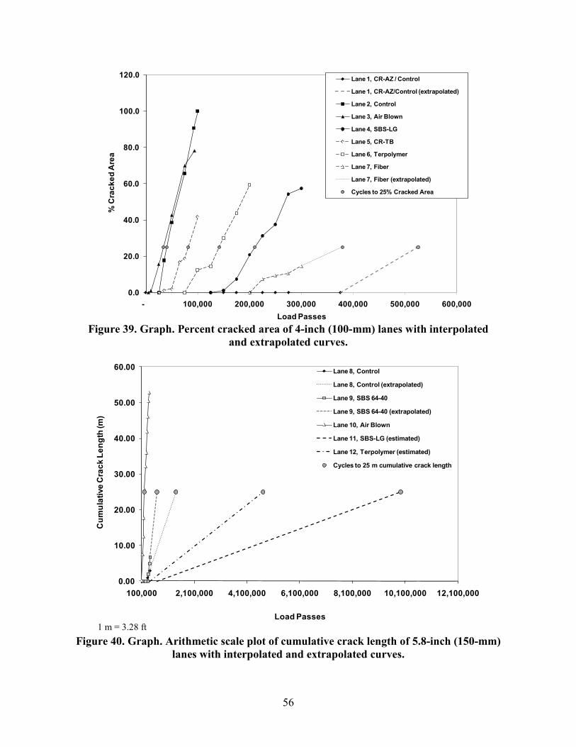
56

Figure 39. Graph. Percent cracked area of 4-inch (100-mm) lanes with interpolated

and extrapolated curves.

1 m = 3.28 ft

Figure 40. Graph. Arithmetic scale plot of cumulative crack length of 5.8-inch (150-mm) lanes with interpolated and extrapolated curves.

0.0

20.0

40.0

60.0

80.0

100.0

120.0

- 100,000 200,000 300,000 400,000 500,000 600,000

% C

rack

ed A

rea

Load Passes

Lane 1, CR-AZ / Control

Lane 1, CR-AZ/Control (extrapolated)

Lane 2, Control

Lane 3, Air Blown

Lane 4, SBS-LG

Lane 5, CR-TB

Lane 6, Terpolymer

Lane 7, Fiber

Lane 7, Fiber (extrapolated)

Cycles to 25% Cracked Area

0.00

10.00

20.00

30.00

40.00

50.00

60.00

100,000 2,100,000 4,100,000 6,100,000 8,100,000 10,100,000 12,100,000

Cum

ulat

ive

Cra

ck L

engt

h (m

)

Load Passes

Lane 8, Control

Lane 8, Control (extrapolated)

Lane 9, SBS 64-40

Lane 9, SBS 64-40 (extrapolated)

Lane 10, Air Blown

Lane 11, SBS-LG (estimated)

Lane 12, Terpolymer (estimated)

Cycles to 25 m cumulative crack length

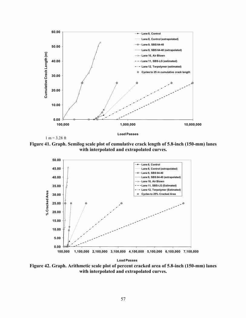
57

1 m = 3.28 ft

Figure 41. Graph. Semilog scale plot of cumulative crack length of 5.8-inch (150-mm) lanes with interpolated and extrapolated curves.

Figure 42. Graph. Arithmetic scale plot of percent cracked area of 5.8-inch (150-mm) lanes

with interpolated and extrapolated curves.

0.00

10.00

20.00

30.00

40.00

50.00

60.00

100,000 1,000,000 10,000,000

Cum

ulat

ive

Cra

ck L

engt

h (m

)

Load Passes

Lane 8, Control

Lane 8, Control (extrapolated)

Lane 9, SBS 64-40

Lane 9, SBS 64-40 (extrapolated)

Lane 10, Air Blown

Lane 11, SBS-LG (estimated)

Lane 12, Terpolymer (estimated)

Cycles to 25 m cumulative crack length

0.00

5.00

10.00

15.00

20.00

25.00

30.00

35.00

40.00

45.00

50.00

100,000 1,100,000 2,100,000 3,100,000 4,100,000 5,100,000 6,100,000 7,100,000

% C

rack

ed A

rea

Load Passes

Lane 8, ControlLane 8, Control (extrapolated)Lane 9, SBS 64-40Lane 9, SBS 64-40 (extrapolated)Lane 10, Air BlownLane 11, SBS-LG (Estimated)Lane 12, Terpolymer (Estimated)Cycles to 25% Cracked Area

58

Figure 43. Graph. Semilog scale plot of percent cracked area of 5.8-inch (150-mm) lanes

with interpolated and extrapolated curves.

Bottom-Up Cracking Evaluation

Cores taken from the loaded area of the fatigue loaded sections were examined to confirm that cracks were initiating and then propagating from the bottom of the asphalt layer to the top. Figure 44 shows X-ray computed tomography images of a core taken from a fatigue cracking section. Crack width was larger at the bottom and became thinner toward the surface. Cores from lane 1, with composite pavement of gap-graded CR-AZ above dense graded PG70-22 mix, are shown in figure 45 and indicate that cracks began at the bottom and propagated through the dense-graded PG70-22 mixture, ultimately being arrested or slowed by the CR-AZ layer.

Figure 44. Photo. X-ray computed tomography image slices of an ALF core.

0.00

5.00

10.00

15.00

20.00

25.00

30.00

35.00

40.00

45.00

50.00

100,000 1,000,000 10,000,000

% C

rack

ed A

rea

Load Passes

Lane 8, ControlLane 8, Control (extrapolated)Lane 9, SBS 64-40Lane 9, SBS 64-40 (extrapolated)Lane 10, Air BlownLane 11, SBS-LG (Estimated)Lane 12, Terpolymer (Estimated)Cycles to 25% Cracked Area

59

Figure 45. Photo. Cores taken from lane 1.

Rutting in Fatigue Sections

Rutting occurred and was measured in the fatigue loading sections. The data show smaller rut depth magnitude between 0.16 and 0.32 inches (4 and 8 mm) due to lateral wander and unknown aging effects. Figure 46 and table 27 show the rutting measured in the 4-inch (100-mm)-thick sections during the 66 °F (19 °C) fatigue test. Lane 5 (CR-TB), which performed best during the high-temperature 147 and 165 °F (64 and 74 °C) tests, had the largest and fastest rutting. The other lanes tended to exhibit almost identical behavior up until about 50,000 cycles and then began to diverge. In lane 3 (air blown), rutting increased very rapidly. Lane 4 (SBS-LG) exhibited the best rutting, and lane 6 (terpolymer), which exhibited the worst rutting during the high-temperature tests, was a moderate performer. All of the lanes began the fatigue test during the same year, after about 2 years of aging, but some began early in February while others began in December.

60

1 mm = 0.039 inches Figure 46. Graph. Rut depths for 4-inch (100-mm) lanes at 66 °F (19 °C).

Table 27. Rut depth in 4-inch (100-mm) fatigue crack sections. Lane 1, CR-AZ/

PG70-22 Lane 2,

PG70-22 Lane 3,

Air Blown Lane 4, SBS-LG

Lane 5, CR-TB

Lane 6, Terpolymer

Passes

Rut Depth (mm) Passes

Rut Depth (mm) Passes

Rut Depth (mm) Passes

Rut Depth (mm) Passes

Rut Depth (mm) Passes

Rut Depth (mm)

500 1.4 1,000 1.4 500 1.7 1,000 1.6 500 4.1 500 1.8 1,000 1.7 5,000 2.4 1,000 2.3 5,000 2.5 1,000 5.2 1,000 2.4 5,000 2.7 10,000 2.8 5,000 2.6 10,000 2.9 5,000 6.9 5,000 3.3 10,000 3.1 25,000 3.1 10,000 3.4 25,000 3.7 10,000 7.1 10,000 3.7 25,000 3.7 50,000 4.4 25,000 3.4 50,000 4.1 25,000 7.7 19,400 4.1 50,000 4.4 75,000 5.2 50,000 4.5 75,000 4.5 50,000 8.2 50,000 4.7 75,000 5.1 100,000 6.4 75,000 9.6 100,000 4.8 75,000 8.9 75,000 5.6

100,000 5.4 — — 93,500 10.6 126,200 5.2 100,000 10.1 96,530 6.6 125,000 5.7 — — — — 150,000 5.8 — — 150,000 9.9 150,000 6.0 — — — — 175,000 6.3 — — 175,000 10.2 175,000 6.4 — — — — 200,000 6.9 — — 200,000 10.5 200,000 6.5 — — — — 250,000 8.6 — — — — 225,000 6.7 — — — — — — — — — — 250,000 7.3 — — — — — — — — — — 275,000 6.8 — — — — — — — — — —

1 mm = 0.039 inches — Indicates test data were not measured because loading had ended.

0.0

2.0

4.0

6.0

8.0

10.0

12.0

0 50,000 100,000 150,000 200,000 250,000 300,000 350,000

ALF Passes

Rut

Dep

th, m

m

Lane 1, CR-AZ / Control, March 2004Lane 2, Control, October 2004Lane 3, Air Blown, December 2004Lane 4, SBS-LG, October 2004Lane 5, CR-TB, February 2004Lane 6, Terpolymer, December 2004

61

Figure 47 and table 28 show the rutting measured in the 5.8-inch (150-mm)-thick sections during the 66 °F (19 °C) fatigue tests. Lane 9 (SBS 64-40), which exhibited the largest amount of rutting during the high-temperature tests at 147 °F (64 °C), provided moderate performance under the intermediate temperatures and wander conditions. It is unknown whether this was due to lane 9 being tested in 2007 rather than with the others in 2005. Lane 11 (SBS-LG) was also tested in 2007, 2 years after the other lanes, and exhibited the best rutting performance. Lane 10 (air blown) clearly performed worst in terms of rutting under the high-temperature zero wander conditions and the intermediate-temperature lateral wander conditions.

1 mm = 0.039 inches

Figure 47. Graph. Rut depths for 5.8-inch (150-mm) lanes at 66 °F (19 °C).

62

Table 28. Rut depth in 5.8-inch (150-mm) fatigue crack sections. Lane 8,

PG70-22 Lane 9,

SBS 64-40 Lane 10,

Air Blown Lane 11, SBS-LG

Lane 12, Terpolymer

Passes

Rut Depth (mm) Passes

Rut Depth (mm) Passes

Rut Depth (mm) Passes

Rut Depth (mm) Passes

Rut Depth (mm)

1,000 0.83 1,000 1.48 1,000 1.00 1,000 1.13 500 0.78 5,000 1.26 10,000 4.14 5,000 2.35 10,000 1.61 1,000 1.26

10,000 2.00 25,000 4.57 10,000 2.96 25,000 1.18 5,000 1.48 25,000 2.61 50,000 4.40 25,000 4.01 50,000 2.13 10,000 1.87 50,000 3.40 75,000 4.83 50,000 5.05 75,000 2.39 25,000 2.35 75,000 3.66 100,000 4.40 75,000 5.79 100,000 2.53 50,000 2.79

107,000 3.88 125,000 4.53 100,000 6.27 125,000 2.74 100,000 3.18 125,000 5.62 150,000 4.62 125,000 7.45 150,000 2.74 100,000 3.27 150,000 4.66 175,000 4.66 150,000 7.53 175,000 2.87 125,000 3.48 175,000 5.23 200,000 4.92 175,000 8.32 200,000 2.96 150,000 3.88 203,000 5.44 225,000 5.40 200,000 8.93 225,000 2.96 175,000 3.66 225,000 5.75 250,000 5.40 230,000 9.01 250,000 3.09 200,000 3.79 250,000 5.79 275,000 5.23 250,000 9.36 275,000 3.31 225,000 3.83 275,000 6.01 300,000 5.49 275,000 9.71 300,000 3.31 250,000 4.22 300,000 6.31 325,000 5.31 300,000 9.67 310,000 3.44 300,000 4.75 325,000 6.40 350,000 5.57 325,000 9.75 310,000 3.53 325,000 5.05 350,000 6.18 375,000 5.57 350,000 9.97 350,000 3.83 350,000 5.27 375,000 6.27 400,000 5.75 375,000 10.15 375,000 3.83 375,000 5.27 400,000 6.53 475,000 6.23 — — 400,000 3.83 400,000 5.36 425,000 6.79 — — — — 425,000 3.83 — — 450,000 6.97 — — — — 450,000 3.83 — — 475,000 7.66 — — — — 500,000 3.79 — —

— — — — — — 575,000 3.79 — — — — — — — — 600,000 3.88 — — — — — — — — 625,000 4.09 — — — — — — — — 650,000 4.22 — — — — — — — — 673,600 4.22 — —

1 mm = 0.039 inches — Test data were not measured because loading had ended.

Anomalous Rutting Performance of Lane 6

A review of the 147 °F (64 °C) rutting performance of the terpolymer sections in figure 24 and figure 26 shows the rutting in 4-inch (100-mm) lane 6 was significantly larger than other lanes of this thickness. However, the rutting performance of 5.8-inch (150-mm) lane 12 was the smallest and best of that thickness. The rutting performance of 4-inch (100-mm) lane 6 terpolymer appears to be an anomaly and warrants discussion. Earlier research indicated that it is possible to improve laboratory fatigue and permanent deformation performance with this modifier.(50)

63

The performance of the 5.8-inch (150-mm) lane 12 terpolymer is more in line with expectations, and there does not appear to be enough evidence to suspect anomalous performance in that lane. Youtcheff et al. published an investigation of the performance of 11 modified asphalts in the 2004 Eurasphalt and Eurobitume Conference.(50) The rut resistance was measured using the French pavement rut tester (PRT) and simple shear tester (SST) RSCH, and fatigue was characterized using four-point bending beam fatigue. Moisture damage and permanent deformation were evaluated using Hamburg wheel tracking (HWT). A list of the binders, polymer content, Superpave® PG, and zero shear viscosity (ZSV) are provided in table 29, where terpolymer polymer modifier is also designated by the DuPont™ trade name Elvaloy®. The performance of the mixtures in the French PRT is given in table 29. The terpolymer performed well with smaller rut depth at a given numbers of cycles with some statistical similarities compared to other mixtures. The permanent deformation performance in the SST RSCH is provided in table 30, which shows the terpolymer modified mixture again performed above other binders with some statistical similarities compared to other mixtures. Table 31 lists the fatigue performance in strain-controlled flexural beam fatigue tests, showing the terpolymer modified binder having the best performance at both strain levels. HWT rut depth curves in the paper also show terpolymer having the smallest rut depth at all cycles.(50)

Table 29. Unmodified and modified binders studied by Youtcheff et al.(50)

Name of Asphalt

Polymer Content (percent) PG

ZSV 58 °C (Pa·s)

ZSV 70 °C (Pa·s)

Unmodified PG64 Unmodified PG70-22

0 0

64-28 70-22

903 1,666

183 327

Air-blown asphalt 0.0 70-28 3,268 530 Ethylene terpolymer (Elvaloy®) 2.2 76-28 6,642 1,514 SBS linear grafted 3.75 70-28 2,539 490 SBS linear 3.75 70-28 2,088 399 SBS radial grafted 3.25 70-28 2,078 397 Ethylene vinyl acetate (EVA) 5.5 64/70-28 7,552 240 EVA grafted 5.5 70-28 7,267 496 Ethylene styrene interpolymer (ESI) 5.0 76-28 2,688 625 Chemically modified crumb rubber asphalt (CMCRA) 5.0 76-28 4,304 766

°F = 1.8(°C) + 32

64

Table 30. French PRT rutting performance of binders studied by Youtcheff et al.(50)

Asphalt Binder or Mixture Designation

DSR after RTFO Aging French PRT after 2 h

of STOA

High-Temperature PG (°C)

|G*|/sin at 70 °C (Pa) Rut Depth at 70 °C (percent) 10.0 radians/s 0.9 radians/s 6,000 Passes 20,000 Passes

Elvaloy® 77 4,110 753 6.5 7.9 Air blown 74 3,870 439 6.8 9.0 CMCRA 76 4,510 566 6.8 9.7 EVA 69 1,910 203 7.1 9.4 SBS radial grafted 71 2,680 312 7.4 8.9 EVA grafted 74 3,440 394 7.5 10.4 ESI 76 4,030 500 7.6 9.2 SBS linear grafted 72 2,880 361 8.2 10.3 PG70-22 71 2,640 260 8.3 10.6 SBS linear 72 2,710 309 8.5 10.5 PG64-28 67 1,570 151 12.1 16.0

°F = 1.8(°C) + 32 1 Pa = 0.000145 psi STOA = Short-term oven aging.

Table 31. Flexural beam fatigue performance of binders studied by Youtcheff et al.(50)

Asphalt Mixture

Number of Cycles to Failure Interpolated Actual Fatigue Data |G*|sin at

19 °C, 10 radians/s (MPa)

At 1,000 microstrains

At 500 microstrains

Elvaloy® 97,389 498,993 1.46 SBS linear grafted 9,911 323,479 1.95 SBS radial grafted 12,372 278,558 1.93 SBS linear 8,774 163,332 1.91 ESI 10,301 135,311 0.61 EVA 7,147 130,817 1.01 Air-blown 7,614 101,436 1.61 CMCRA 4,158 64,751 2.55 EVA grafted 7,183 51,709 1.36 PG64-28 5,323 37,885 2.53 PG70-22 3,144 15,877 2.31

°F = 1.8(°C) + 32 1 MPa = 145 psi

The circumstances of the construction were explored, and a forensic investigation was conducted to avoid any unsubstantiated speculation about the causes of the poor performance. First, both lanes 6 and 12 were constructed on the same date from the same run of plant production. The weather on the day of construction and all relevant preceding days was very good, without any notable rainfall or cold weather. This likely eliminates the possibility that the aggregate stockpiles were saturated when the mix was produced. Chemically speaking, there is no reason to suspect negative interaction of hydrated lime with the terpolymer modifier. The ranking of the rut depths at 165 °F (74 °C) from tests several years after the 147 °F (64 °C) rutting tests was nearly identical; lane 6 had the worst rutting at both points in time. This indicates that the

δ

δ

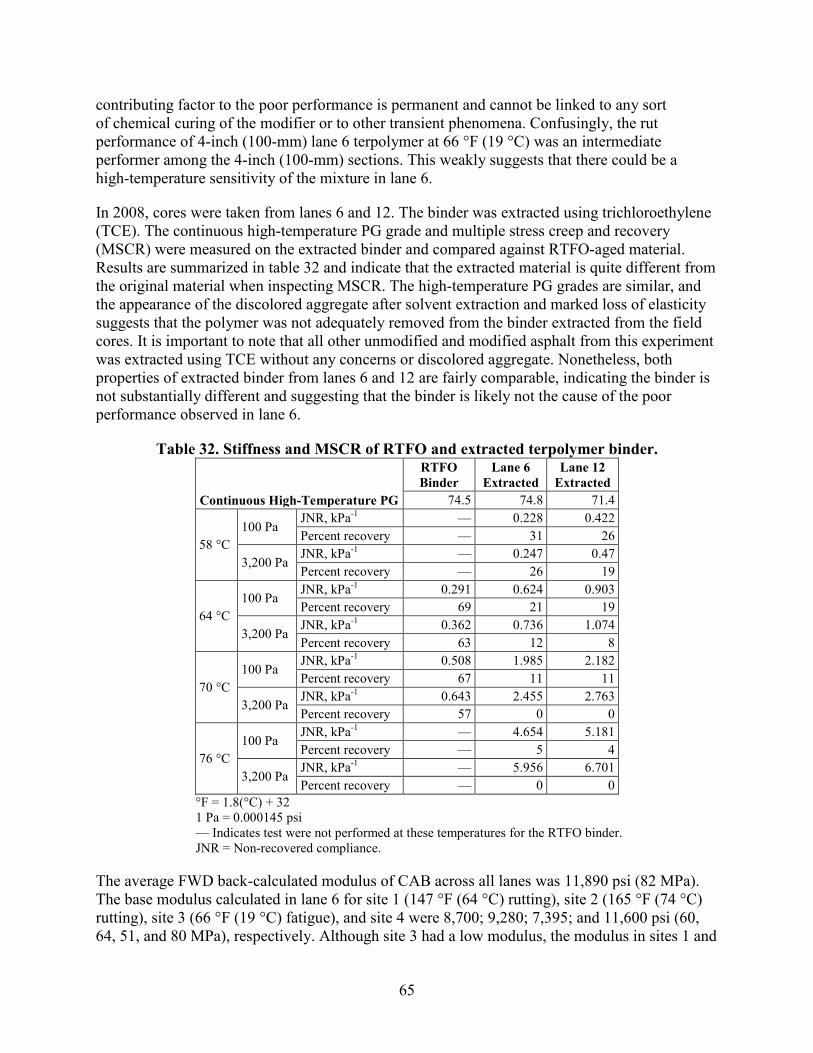
65

contributing factor to the poor performance is permanent and cannot be linked to any sort of chemical curing of the modifier or to other transient phenomena. Confusingly, the rut performance of 4-inch (100-mm) lane 6 terpolymer at 66 °F (19 °C) was an intermediate performer among the 4-inch (100-mm) sections. This weakly suggests that there could be a high-temperature sensitivity of the mixture in lane 6.

In 2008, cores were taken from lanes 6 and 12. The binder was extracted using trichloroethylene (TCE). The continuous high-temperature PG grade and multiple stress creep and recovery (MSCR) were measured on the extracted binder and compared against RTFO-aged material. Results are summarized in table 32 and indicate that the extracted material is quite different from the original material when inspecting MSCR. The high-temperature PG grades are similar, and the appearance of the discolored aggregate after solvent extraction and marked loss of elasticity suggests that the polymer was not adequately removed from the binder extracted from the field cores. It is important to note that all other unmodified and modified asphalt from this experiment was extracted using TCE without any concerns or discolored aggregate. Nonetheless, both properties of extracted binder from lanes 6 and 12 are fairly comparable, indicating the binder is not substantially different and suggesting that the binder is likely not the cause of the poor performance observed in lane 6.

Table 32. Stiffness and MSCR of RTFO and extracted terpolymer binder.

Continuous High-Temperature PG

RTFO Binder

Lane 6 Extracted

Lane 12 Extracted

74.5 74.8 71.4

58 °C 100 Pa

JNR, kPa-1 — 0.228 0.422 Percent recovery — 31 26

3,200 Pa JNR, kPa-1 — 0.247 0.47 Percent recovery — 26 19

64 °C 100 Pa

JNR, kPa-1 0.291 0.624 0.903 Percent recovery 69 21 19

3,200 Pa JNR, kPa-1 0.362 0.736 1.074 Percent recovery 63 12 8

70 °C 100 Pa

JNR, kPa-1 0.508 1.985 2.182 Percent recovery 67 11 11

3,200 Pa JNR, kPa-1 0.643 2.455 2.763 Percent recovery 57 0 0

76 °C 100 Pa

JNR, kPa-1 — 4.654 5.181 Percent recovery — 5 4

3,200 Pa JNR, kPa-1 — 5.956 6.701 Percent recovery — 0 0

°F = 1.8(°C) + 32 1 Pa = 0.000145 psi — Indicates test were not performed at these temperatures for the RTFO binder. JNR = Non-recovered compliance.

The average FWD back-calculated modulus of CAB across all lanes was 11,890 psi (82 MPa). The base modulus calculated in lane 6 for site 1 (147 °F (64 °C) rutting), site 2 (165 °F (74 °C) rutting), site 3 (66 °F (19 °C) fatigue), and site 4 were 8,700; 9,280; 7,395; and 11,600 psi (60, 64, 51, and 80 MPa), respectively. Although site 3 had a low modulus, the modulus in sites 1 and

66

2 were not dramatically softer than other lanes and sites. For example, the stiffness of the four sites in lane 3 (air blown) were 7,975; 7,830; 7,395; and 8,845 psi (55, 54, 51, and 61 MPa). Again, this lane was unmodified asphalt and did not experience rutting of the magnitude observed in lane 6.

Figure 48 shows a schematic layout of where cores were taken after construction and for a second set of forensic cores. The air void contents of the six cores taken after construction at stations 23, 80, and 139 using saturated surface dry (SSD) AASHTO T 166 of the 4-inch (100-mm) lane 6 were 6.6, 5.5, 7.2, 6.4, 7.0, and 5.8 percent for an average of 6.42 percent and a standard deviation of 0.67 percent.(45) When more cores were taken later from lane 6, the average air void content was 7.6 percent. This was not the largest air void content of the 4-inch (100-mm) sections. The highest average air void content was lane 2, where the average air void content of the six post-construction cores was 7.8 percent with a standard deviation of 0.86 percent. When more cores were taken from lane 2 over time, the average air void content was 8.0 percent. This lane was unmodified asphalt and did not experience rutting of the magnitude observed in lane 6. The average air void content of the 5.8-inch (150-mm) lane 12 terpolymer was 5.9 percent with a standard deviation of 0.91 percent.

Figure 48. Illustration. Schematic layout of ALF lane construction.

67

FHWA collaborated with a polymer manufacturer and an asphalt modifying company and supplier, who supplied the terpolymer and modified binder for the experiment, to explore a second set of forensic cores from lane 2 (4 inches (100 mm), PG70-22), lane 6 (4 inches (100 mm), terpolymer), and lane 12 (5.8 inches (150 mm), terpolymer). It was suggested to quantify differences between air void content measured by means of SSD (AASHTO T 166) and CoreLok® (AASHTO T 331).(45,51) Three cores were taken along the centerline of each lane in the rutting sections between sites 1 and 2 at stations 34, 46, and 58. Three cores from each lane were also taken from the fatigue cracking sections between sites 3 and 4 at stations 100, 112, and 124, for a total of 18 cores. The results of FHWA’s tests are shown in table 33.

Table 33. FHWA forensic test results for lane 2, 6, and 12 air void content and water absorption from SSD and CoreLok®.

Core Location

AASHTO T 166(45) (SSD)

Air Void (percent)

AASHTO T 331(51) (CoreLok®) Air Void (percent)

Difference in Air Void (percent)

AASHTO T 166(45) Water Absorption

(percent)

Lane 2, 4-inch (100- mm) PG70-22

Station 34 9.0 9.9 0.9 2.02 Station 46 6.4 7.1 0.7 0.45 Station 58 6.7 7.3 0.5 0.88 Station 100 6.4 6.9 0.5 0.72 Station 112 6.1 6.8 0.6 0.55 Station 124 6.6 7.3 0.7 0.71 Average 6.9 7.5 0.7 0.9

Lane 6, 4-inch (100- mm) terpolymer

Station 34 7.5 8.4 1.0 2.39 Station 46 7.9 8.6 0.7 2.53 Station 58 8.1 8.8 0.7 2.99 Station 100 8.2 8.9 0.7 2.95 Station 112 7.2 7.9 0.7 2.03 Station 124 7.6 8.1 0.5 2.02 Average 7.7 8.5 0.7 2.5

Lane 12, 5.8-inch (150-mm) terpolymer

Station 34 5.2 6.2 1.0 0.98 Station 46 5.4 5.8 0.4 0.95 Station 58 5.1 5.7 0.7 0.72 Station 100 3.7 4.7 1.0 0.37 Station 112 3.5 4.2 0.6 0.26 Station 124 4.0 4.5 0.5 0.35 Average 4.5 5.2 0.7 0.6

A comparison of the historical SSD air void contents previously described with the second set of forensic cores showed variation but fairly comparable air void contents, with lane 2 having 8 and 6.9 percent, lane 6 having 7.6 and 7.7 percent, and lane 12 having 5.9 and 4.5 percent. As expected, CoreLok® resulted in a larger air void content of 0.7 percent more air voids for all three lanes in the second set of forensic cores. By far, the largest indicator of differences between the anomalous performing lane 6 and better performing lane 12 lay in the water absorption. Lane 6 exhibited over four times larger water absorption than lane 12. Part of that difference may lie in the differences in air void content. However, the air void contents of lanes 2 and 6 were more similar, and the water absorption was still notably higher in lane 6.

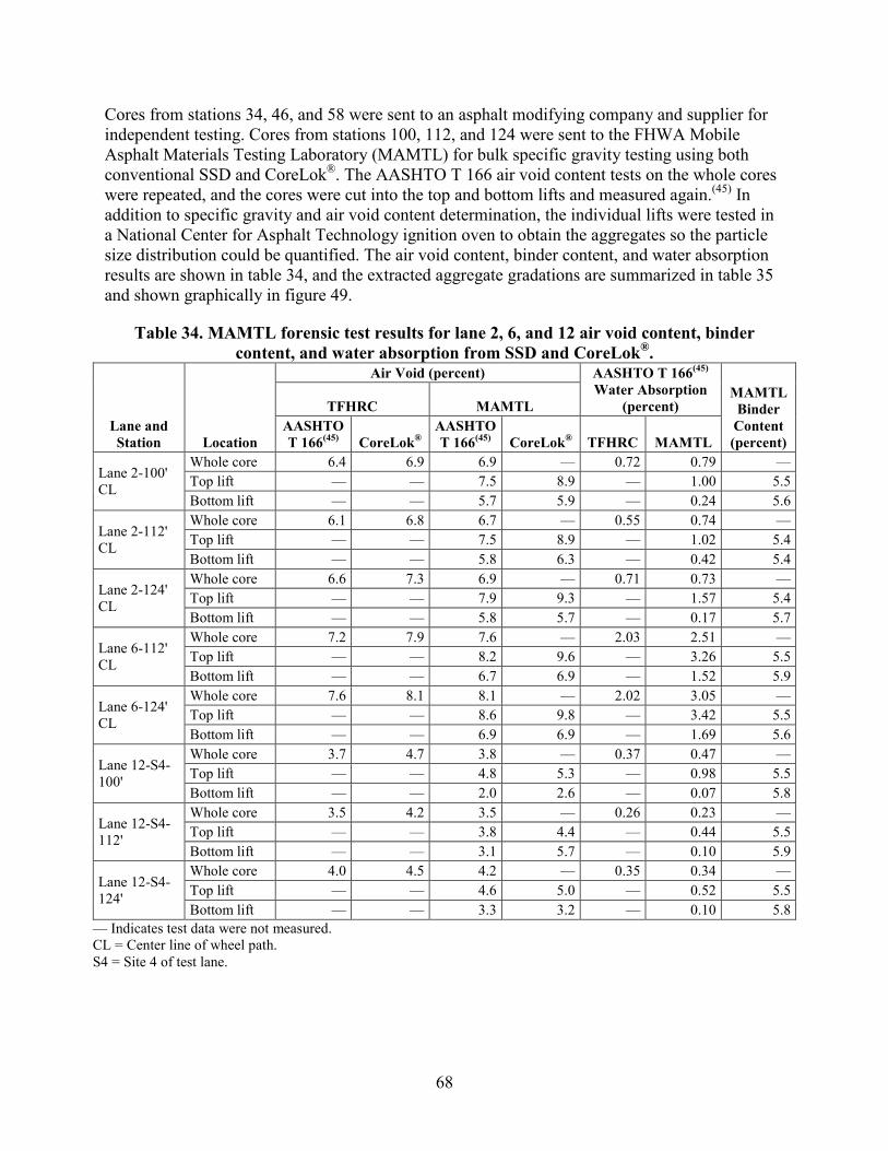
68

Cores from stations 34, 46, and 58 were sent to an asphalt modifying company and supplier for independent testing. Cores from stations 100, 112, and 124 were sent to the FHWA Mobile Asphalt Materials Testing Laboratory (MAMTL) for bulk specific gravity testing using both conventional SSD and CoreLok®. The AASHTO T 166 air void content tests on the whole cores were repeated, and the cores were cut into the top and bottom lifts and measured again.(45) In addition to specific gravity and air void content determination, the individual lifts were tested in a National Center for Asphalt Technology ignition oven to obtain the aggregates so the particle size distribution could be quantified. The air void content, binder content, and water absorption results are shown in table 34, and the extracted aggregate gradations are summarized in table 35 and shown graphically in figure 49.

Table 34. MAMTL forensic test results for lane 2, 6, and 12 air void content, binder content, and water absorption from SSD and CoreLok®.

Lane and Station Location

Air Void (percent) AASHTO T 166(45) Water Absorption

(percent) MAMTL

Binder Content (percent)

TFHRC MAMTL AASHTO T 166(45) CoreLok®

AASHTO T 166(45) CoreLok® TFHRC MAMTL

Lane 2-100' CL

Whole core 6.4 6.9 6.9 — 0.72 0.79 — Top lift — — 7.5 8.9 — 1.00 5.5 Bottom lift — — 5.7 5.9 — 0.24 5.6

Lane 2-112' CL

Whole core 6.1 6.8 6.7 — 0.55 0.74 — Top lift — — 7.5 8.9 — 1.02 5.4 Bottom lift — — 5.8 6.3 — 0.42 5.4

Lane 2-124' CL

Whole core 6.6 7.3 6.9 — 0.71 0.73 — Top lift — — 7.9 9.3 — 1.57 5.4 Bottom lift — — 5.8 5.7 — 0.17 5.7

Lane 6-112' CL

Whole core 7.2 7.9 7.6 — 2.03 2.51 — Top lift — — 8.2 9.6 — 3.26 5.5 Bottom lift — — 6.7 6.9 — 1.52 5.9

Lane 6-124' CL

Whole core 7.6 8.1 8.1 — 2.02 3.05 — Top lift — — 8.6 9.8 — 3.42 5.5 Bottom lift — — 6.9 6.9 — 1.69 5.6

Lane 12-S4-100'

Whole core 3.7 4.7 3.8 — 0.37 0.47 — Top lift — — 4.8 5.3 — 0.98 5.5 Bottom lift — — 2.0 2.6 — 0.07 5.8

Lane 12-S4-112'

Whole core 3.5 4.2 3.5 — 0.26 0.23 — Top lift — — 3.8 4.4 — 0.44 5.5 Bottom lift — — 3.1 5.7 — 0.10 5.9

Lane 12-S4-124'

Whole core 4.0 4.5 4.2 — 0.35 0.34 — Top lift — — 4.6 5.0 — 0.52 5.5 Bottom lift — — 3.3 3.2 — 0.10 5.8

— Indicates test data were not measured. CL = Center line of wheel path. S4 = Site 4 of test lane.

69

Table 35. MAMTL forensic test results for lane 2, 6, and 12 extracted aggregate gradation.

Sieve Size Lane 2, Total

Percent Passing Lane 6, Total

Percent Passing Lane 12, Total

Percent Passing Limits Std. (mm) Average Std. Dev. Average Std. Dev. Average Std. Dev. Upper Lower 1 inch 25 100.0 0.0 100.0 0.0 100.0 0.0

3/4 inch 19 100.0 0.0 100.0 0.0 100.0 0.0 1/2 inch 12.5 95.3 0.8 96.5 0.5 96.2 0.5 3/8 inch 9.5 85.1 1.0 89.0 0.7 88.3 1.9 No. 4 4.75 55.9 1.8 61.7 1.2 61.7 2.6 58 52

No. 8 2.36 36.0 0.9 39.5 1.2 40.6 1.9 No. 16 1.18 25.2 0.6 27.5 0.8 28.7 1.3 No. 30 0.600 18.5 0.4 20.1 0.6 21.4 1.0 19 15

No. 50 0.300 13.7 0.3 14.8 0.5 16.0 0.8 No. 100 0.150 9.9 0.2 10.7 0.4 11.8 0.6 No. 200 0.075 6.8 0.1 7.4 0.4 8.3 0.4 7 5.6

1 mm = 0.039 inches Note: Blank cells indicate there were no gradation limits at the particular sieve size.

1 mm = 0.039 inches

Figure 49. Graph. Particle size distribution of extracted aggregate for lanes 2, 6, and 12.

Rutting in Unbound Layers

The rutting in the asphalt layers was calculated as a percentage of the total surface rutting. The differences in this percentage were evaluated to explore how temperature and wheel wander influence the distribution of permanent deformations in the unbound layers and AC layers. The percentage of total rutting in the asphalt layers for the 4- and 5.8-inch (100- and 150-mm) lanes at 147 °F (64 °C) and the 4-inch (100-mm) lanes at 165 °F (74 °C) without wander was, on

0.0

10.0

20.0

30.0

40.0

50.0

60.0

70.0

80.0

90.0

100.0

0 0.5 1 1.5 2 2.5 3 3.5 4 4.5

Perc

ent P

assin

g (%

)

Sive Size (mm) ̂ 0.45

Lane 2 Control 100 mm

Lane 12 Terpolymer 150 mm

Lane 6 Terpolymer 100 mm

Target

70

average, 54 percent with a standard deviation of 17 percent. When the temperature was dropped to 113 °F (45 °C) for the 5.8-inch (150-mm) lanes without wander, the percentage of total rutting in the asphalt layer was, on average, 51 percent with a standard deviation of 18 percent. When the temperature was 66 °F (19 °C) with wheel wander, the percentage of rutting in the 4- and 5.8-inch (100- and 150-mm) asphalt layers was, on average, 31 percent with a standard deviation of 9 percent. The combination of lower temperatures and wheel wander appears to increase rutting in the unbound layers and decrease rutting in the asphalt layers.

NUMERICAL AND STATISTICAL CONSEQUENCES OF LAYOUT AND PERFORMANCE

This APT experiment was designed with mixtures having identical aggregate and identical mix design with different asphalt binders to allow comparisons to be made between full-scale fatigue cracking and rutting performance and binder specification parameters. The experiment also contains pavement configurations having different thicknesses and stiffnesses (by varying the binder) that allow mechanistic-empirical pavement performance models to be evaluated. Comparisons can be made between measured performance, material property inputs, and design and analysis model outputs that can predict relative and absolute performance.

However, in this experimental design, the initiative of one aspect of the experiment impacts the numerical and statistical strengths of another initiative. A divided subset of pavement test sections by thickness (4 and 5.8 inches (100 and 150 mm)) and the presence of unique types of mixtures and pavements sections (CR-AZ/PG70-22, fiber, CR-TB, and SBS 64-40) that do not have counterparts with a different thickness affect the conditioning of the binder-only variable dataset and the pavement thickness variable dataset. In other words, a statistically sufficient number of data points having only one variable among them are ideal. A total of 12 data points, which correlates to the number of test lanes, is a relatively good number. However, all 12 data points cannot be used for every type of performance comparison, as illustrated in figure 50.

Figure 50. Diagram. Numerical tree of subsets of available comparative data points.

71

ALF PTF can accommodate 12 lanes, but 7 of the lanes are 4 inches (100 mm) thick, and 5 lanes are 5.8 inches (150 mm) thick. The data from these two sets cannot be easily combined for direct comparison of binder properties against full-scale ALF performance or laboratory mix tests because thickness and constructed density of those lanes confound the binder type variable. The lane 7 fiber mixture cannot be characterized by means of binder tests because the scale of the fibers relative to the size of binder-test specimens is too large for a representative sample. However, the performance of this lane can be utilized for comparisons between laboratory tests on asphalt-aggregate mixtures and full-scale ALF performance. The performance of lane 6 (terpolymer) must be taken with some caution. As shown in the previous section, it had the worst performance of the 4-inch (100-mm) sections but the best performance of 5.8-inch (150-mm) sections, and this poor performance was not within reasonable expectations based on historical binder and mixture tests on the materials. Lane 1 (CR-AZ/PG70-22) is a composite section, which excludes the data from being part of the direct comparison between binder properties and full-scale performance. Naturally, this creates numerical and statistical challenges when it comes to sufficient justification to claim one binder specification parameter is any stronger or weaker than another.

ANALYTICAL PLAN: HOW WILL ONE CANDIDATE BINDER SPECIFICATION PARAMETER BE COMPARED AGAINST ANOTHER?

A variety of comparisons and quantitative techniques were used to compare candidate binder specification parameters against mixture performance and full-scale pavement performance. More than one technique summarized in the list below was used because a large number of data points were not available for making comparisons and judging the strength of various material properties against others. Ultimately, the different techniques were combined into a single composite score for simplified cross comparison. The techniques are as follows:

• Proportional relationship (+) or inverse relationship (–) compared to expected direction.

o Basic linear regression slope (arithmetic, semilog, or log-log, as necessary).

o Kendall’s tau measure of association score, -1 < < +1.

• ANOVA significance of the regression slope, t-statistic, and p-value.

• Significance of the Kendall’s tau association, test for independence.

• Coefficient of determination, R2, and correlation coefficient, R.

• Composite score consisting of contributions from the above characteristics.

First, the direction of the relationship in either the inverse direction or proportional direction was tested and compared against the direction expected for a particular set of binder parameters and pavement performance quantity. For example, an inverse relationship would be expected for two variables such as amount of cracking in the field versus number of cycles to reach failure in the laboratory. Conversely, a proportional relationship would be expected for two variables such as rut depth at a fixed number of passes versus permanent strain at a fixed number of cycles in

τK

72

the laboratory. The direction of the relationship can be quantified by the linear regression slope, correlation coefficient, and the score calculated by the Kendall’s tau measure of association.

The Kendall’s tau measure of association is a distribution-free, or non-parametric, rank-correlation parameter.(52,53) The parameter is better suited to small datasets than is the correlation coefficient, R, or the coefficient of determination, R2, which are more appropriate for larger datasets. The score is calculated from paired data. The sets of pairs are ranked in increasing order by one of the columns of values. Calculations are based on concordant and discordant observations in the column of data that was not sorted in rank order. All values below the first row are compared to the value in the first row. If the particular value is greater than the first row value, it is considered a concordant observation. Likewise, if the particular value is less than the first row value, it is considered a discordant value. The process is then repeated, but all observations are made relative to the second row value, then to the third row, and so on until the next to last row. The Kendall’s tau score is calculated as shown in figure 51.

Figure 51. Equation. Kendall’s tau.

Where:

NC = Total number of concordant observations. ND = Total number of discordant observations. n = Total number of data points.

The numerical range of Kendall’s tau is between -1 and +1, where a +1 score indicates perfect agreement or ranking between two datasets and a -1 score indicates perfect disagreement or opposite ranking. A score of 0 indicates complete lack of correspondence or complete independence of one dataset from the other. An advantage of the Kendall’s tau parameter is that its magnitude cannot be dominated by isolated data points. The coefficient of determination, R2, can increase (or decrease) rapidly depending on the location of a single data point and artificially suggest a high (or low) degree of correlation even when there are very few data points in a particular set.

Another advantage of the Kendall’s tau parameter is that the statistical significance of the ranking can be evaluated with a statistical test for the independence of the two datasets based on the NC – ND score and the number of paired data points. The null hypothesis, Ho, of the test is that the two datasets are independent of each other and have no correlation. When a single-sided test is used, the alternative hypothesis, Ha, is that the two variables have a correlation greater or less than zero. The basis for the statistics of the Kendall’s tau test for independence comes from the fact that for a given number of data points, there are a fixed number of ranking permutations where there are more possible outcomes with a near-zero score. If Ho is rejected depending on the chosen level of significance in a two-sided test, the correlation of the two sets can be taken as something other than zero. In other words, if more data points were available, some correlation might be expected.

2

)1( −−= nn

NNK

DCτ

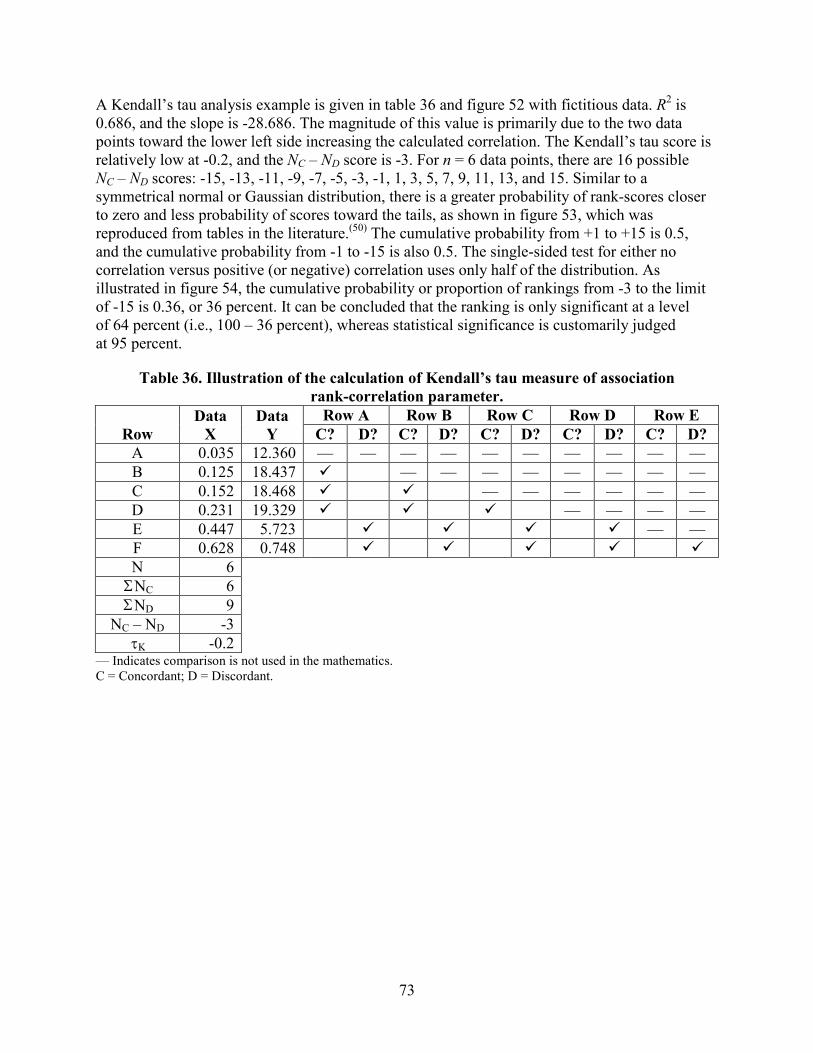
73

A Kendall’s tau analysis example is given in table 36 and figure 52 with fictitious data. R2 is 0.686, and the slope is -28.686. The magnitude of this value is primarily due to the two data points toward the lower left side increasing the calculated correlation. The Kendall’s tau score is relatively low at -0.2, and the NC – ND score is -3. For n = 6 data points, there are 16 possible NC – ND scores: -15, -13, -11, -9, -7, -5, -3, -1, 1, 3, 5, 7, 9, 11, 13, and 15. Similar to a symmetrical normal or Gaussian distribution, there is a greater probability of rank-scores closer to zero and less probability of scores toward the tails, as shown in figure 53, which was reproduced from tables in the literature.(50) The cumulative probability from +1 to +15 is 0.5, and the cumulative probability from -1 to -15 is also 0.5. The single-sided test for either no correlation versus positive (or negative) correlation uses only half of the distribution. As illustrated in figure 54, the cumulative probability or proportion of rankings from -3 to the limit of -15 is 0.36, or 36 percent. It can be concluded that the ranking is only significant at a level of 64 percent (i.e., 100 – 36 percent), whereas statistical significance is customarily judged at 95 percent.

Table 36. Illustration of the calculation of Kendall’s tau measure of association rank-correlation parameter.

Row Data

X Data

Y Row A Row B Row C Row D Row E

C? D? C? D? C? D? C? D? C? D? A 0.035 12.360 — — — — — — — — — — B 0.125 18.437 — — — — — — — — C 0.152 18.468 — — — — — — D 0.231 19.329 — — — — E 0.447 5.723 — — F 0.628 0.748 N 6 NC 6 ND 9

NC – ND -3 -0.2

— Indicates comparison is not used in the mathematics. C = Concordant; D = Discordant.

Σ Σ

τK

74

Figure 52. Graph. Fictitious data with linear regression fit for Kendall’s tau rank

correlation example.

Figure 53. Graph. Possible permutations of rankings for Kendall’s tau.(52)

y = -28.686x + 20.247R2 = 0.6858

0

5

10

15

20

25

0.0 0.2 0.4 0.6 0.8Data "X"

Dat

a "Y

"

-11, 0.028

-9, 0.068

-7, 0.136

-5, 0.235

-3, 0.36

1, 0.5

3, 0.36

5, 0.235

7, 0.136

9, 0.068

11, 0.028

-1, 0.5

13, 0.0083-13, 0.0083

-15, 0.0014 15, 0.00140

0.1

0.2

0.3

0.4

0.5

0.6

-15 -13 -11 -9 -7 -5 -3 -1 1 3 5 7 9 11 13 15

NC - ND Score specifically for n = 6 scenario

Prop

ortio

n of

Ken

dall

Tau

Ran

king

s

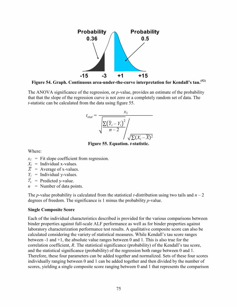
75

Figure 54. Graph. Continuous area-under-the-curve interpretation for Kendall’s tau.(52)

The ANOVA significance of the regression, or p-value, provides an estimate of the probability that that the slope of the regression curve is not zero or a completely random set of data. The t-statistic can be calculated from the data using figure 55.

Figure 55. Equation. t-statistic.

Where: x1 = Fit slope coefficient from regression. Xi = Individual x-values.

= Average of x-values. Yi = Individual y-values.

= Predicted y-value. n = Number of data points.

The p-value probability is calculated from the statistical t-distribution using two tails and n – 2 degrees of freedom. The significance is 1 minus the probability p-value.

Single Composite Score

Each of the individual characteristics described is provided for the various comparisons between binder properties against full-scale ALF performance as well as for binder properties against laboratory characterization performance test results. A qualitative composite score can also be calculated considering the variety of statistical measures. While Kendall’s tau score ranges between -1 and +1, the absolute value ranges between 0 and 1. This is also true for the correlation coefficient, R. The statistical significance (probability) of the Kendall’s tau score, and the statistical significance (probability) of the regression both range between 0 and 1. Therefore, these four parameters can be added together and normalized. Sets of these four scores individually ranging between 0 and 1 can be added together and then divided by the number of scores, yielding a single composite score ranging between 0 and 1 that represents the comparison

Probability0.36

Probability0.5

-3 +1 +15-15

tstat = x1

�∑�Y� i – Yi�2

n – 2�∑(Xi – X�)2

�

76

between the binder candidate parameters against the full-scale ALF performance and the binder candidate parameters against the laboratory performance tests.

Illustration of the Numerical and Statistical Challenges

A dataset that is familiar and generally accepted by most pavement engineers is the Witczak predictive model for dynamic modulus. This dataset is used to illustrate the variety of statistical measures used to evaluate the candidate binder parameters and mixture characterization tests in light of the full-scale ALF rutting and fatigue performance. The |E*| predictive model has been recently reformulated and recalibrated by Bari.(54) There are 7,400 data points of measured and correspondingly predicted dynamic modulus |E*| shown in log-log scale in figure 56 and in arithmetic scale in figure 57. The slope of the regression is 0.964, which is close to the line of equality, with an intercept of 213,624 psi (1,473 MPa). The R2 value of the fit is 0.90 for the log-log data and 0.80 for the arithmetic data. The ratio of the standard error to the standard deviation of observed values SE/SY is 0.32 for the log-log data and 0.45 for the arithmetic data.

Figure 56. Graph. Log-log plot of measured versus predicted dynamic modulus data points

from calibrated Witczak predictive equation.(54)

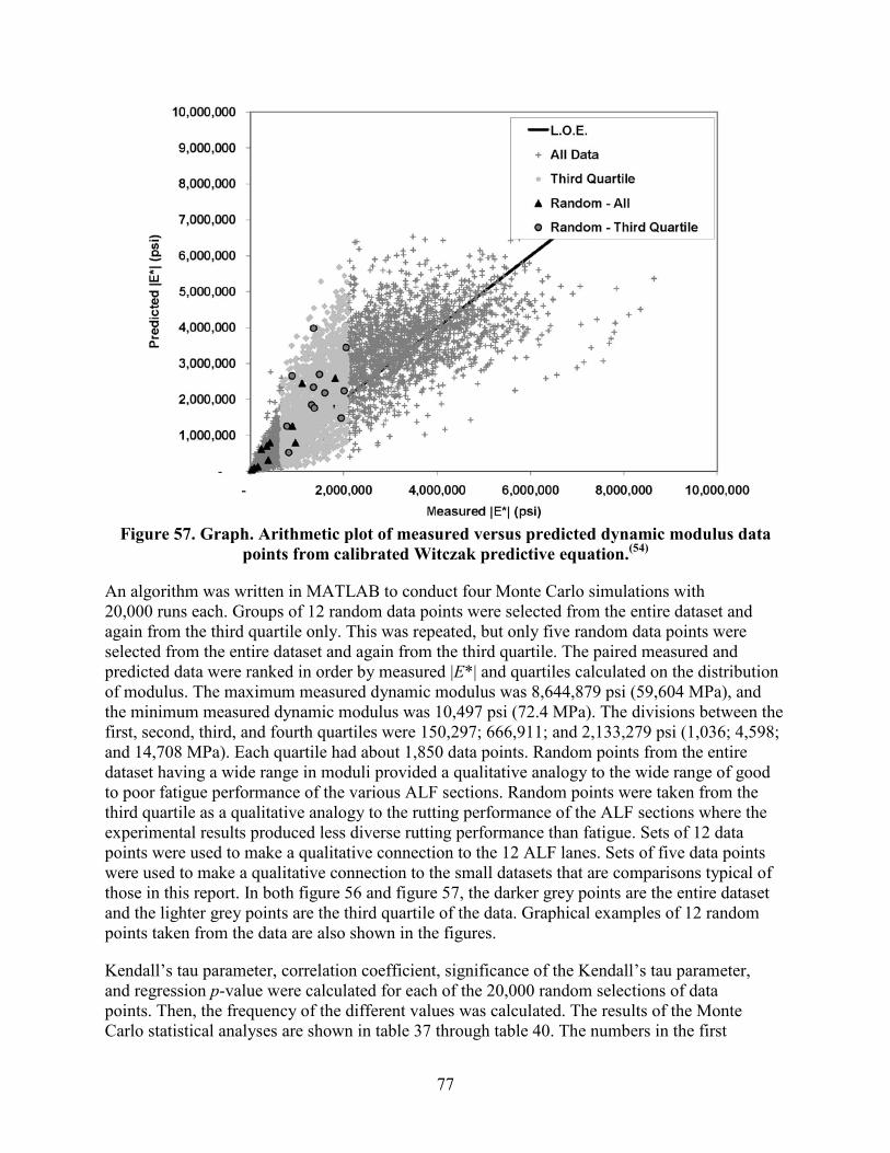
77

Figure 57. Graph. Arithmetic plot of measured versus predicted dynamic modulus data

points from calibrated Witczak predictive equation.(54)

An algorithm was written in MATLAB to conduct four Monte Carlo simulations with 20,000 runs each. Groups of 12 random data points were selected from the entire dataset and again from the third quartile only. This was repeated, but only five random data points were selected from the entire dataset and again from the third quartile. The paired measured and predicted data were ranked in order by measured |E*| and quartiles calculated on the distribution of modulus. The maximum measured dynamic modulus was 8,644,879 psi (59,604 MPa), and the minimum measured dynamic modulus was 10,497 psi (72.4 MPa). The divisions between the first, second, third, and fourth quartiles were 150,297; 666,911; and 2,133,279 psi (1,036; 4,598; and 14,708 MPa). Each quartile had about 1,850 data points. Random points from the entire dataset having a wide range in moduli provided a qualitative analogy to the wide range of good to poor fatigue performance of the various ALF sections. Random points were taken from the third quartile as a qualitative analogy to the rutting performance of the ALF sections where the experimental results produced less diverse rutting performance than fatigue. Sets of 12 data points were used to make a qualitative connection to the 12 ALF lanes. Sets of five data points were used to make a qualitative connection to the small datasets that are comparisons typical of those in this report. In both figure 56 and figure 57, the darker grey points are the entire dataset and the lighter grey points are the third quartile of the data. Graphical examples of 12 random points taken from the data are also shown in the figures.

Kendall’s tau parameter, correlation coefficient, significance of the Kendall’s tau parameter, and regression p-value were calculated for each of the 20,000 random selections of data points. Then, the frequency of the different values was calculated. The results of the Monte Carlo statistical analyses are shown in table 37 through table 40. The numbers in the first

78

column are the edges of the bins used to sort the Monte Carlo values and calculate the frequency distribution.

Table 37. Distribution of Kendall’s tau parameter from Monte Carlo simulations.

Kendall’s Tau Coefficient

12 Points 5 Points Entire Dataset

(percent) Third Quartile

(percent) Entire Dataset

(percent) Third Quartile

(percent -1 0.00 0.00 0.00 0.05 -0.9 0.00 0.00 — — -0.8 0.00 0.00 0.00 0.23 -0.7 0.00 0.00 — — -0.6 0.00 0.00 0.01 0.73 -0.5 0.00 0.00 — — -0.4 0.00 0.00 0.34 0.02 -0.3 0.00 0.04 — — -0.2 0.00 0.10 0.01 0.04 -0.1 0.00 0.33 — — 0 0.00 0.77 0.39 9.45 0.1 0.00 3.11 — — 0.2 0.01 5.29 1.62 16.07 0.3 0.08 9.81 — — 0.4 0.32 20.59 5.89 22.94 0.5 1.87 20.51 — — 0.6 13.18 18.83 17.69 24.63 0.7 32.21 15.58 — — 0.8 39.65 4.10 39.47 18.96 0.9 12.51 0.89 — — 1 0.17 0.06 34.58 6.88

— Indicates that Kendall’s tau coefficient does not exist when five data points are used.

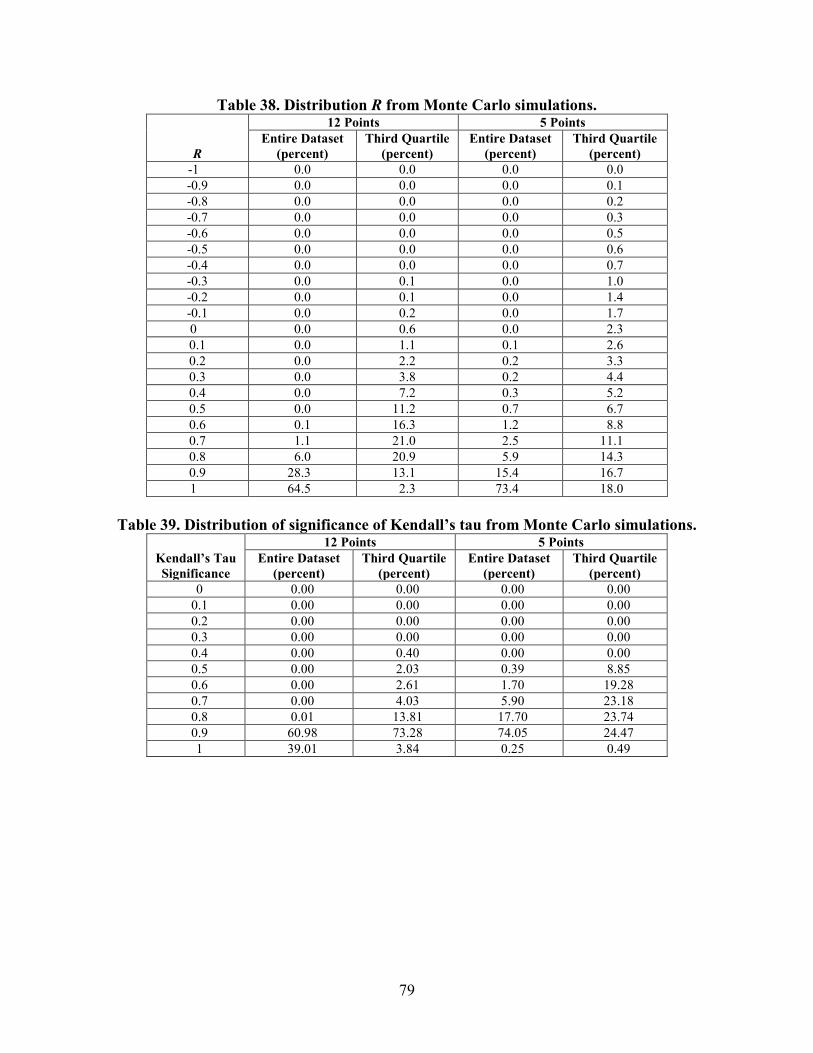
79

Table 38. Distribution R from Monte Carlo simulations.

R

12 Points 5 Points Entire Dataset

(percent) Third Quartile

(percent) Entire Dataset

(percent) Third Quartile

(percent) -1 0.0 0.0 0.0 0.0 -0.9 0.0 0.0 0.0 0.1 -0.8 0.0 0.0 0.0 0.2 -0.7 0.0 0.0 0.0 0.3 -0.6 0.0 0.0 0.0 0.5 -0.5 0.0 0.0 0.0 0.6 -0.4 0.0 0.0 0.0 0.7 -0.3 0.0 0.1 0.0 1.0 -0.2 0.0 0.1 0.0 1.4 -0.1 0.0 0.2 0.0 1.7 0 0.0 0.6 0.0 2.3 0.1 0.0 1.1 0.1 2.6 0.2 0.0 2.2 0.2 3.3 0.3 0.0 3.8 0.2 4.4 0.4 0.0 7.2 0.3 5.2 0.5 0.0 11.2 0.7 6.7 0.6 0.1 16.3 1.2 8.8 0.7 1.1 21.0 2.5 11.1 0.8 6.0 20.9 5.9 14.3 0.9 28.3 13.1 15.4 16.7 1 64.5 2.3 73.4 18.0

Table 39. Distribution of significance of Kendall’s tau from Monte Carlo simulations.

Kendall’s Tau Significance

12 Points 5 Points Entire Dataset

(percent) Third Quartile

(percent) Entire Dataset

(percent) Third Quartile

(percent) 0 0.00 0.00 0.00 0.00

0.1 0.00 0.00 0.00 0.00 0.2 0.00 0.00 0.00 0.00 0.3 0.00 0.00 0.00 0.00 0.4 0.00 0.40 0.00 0.00 0.5 0.00 2.03 0.39 8.85 0.6 0.00 2.61 1.70 19.28 0.7 0.00 4.03 5.90 23.18 0.8 0.01 13.81 17.70 23.74 0.9 60.98 73.28 74.05 24.47 1 39.01 3.84 0.25 0.49

80

Table 40. Distribution of regression significance (1 – p-value) from Monte Carlo simulations.

Regression Significance (1 – p-value)

12 Points 5 Points Entire Dataset

(percent) Third Quartile

(percent) Entire Dataset

(percent) Third Quartile

(percent) 0 0 0 0 0 0.1 0 1 0 4 0.2 0 1 0 4 0.3 0 1 0 4 0.4 0 1 0 5 0.5 0 1 0 5 0.6 0 2 1 6 0.7 0 3 1 8 0.8 0 6 2 12 0.9 0 11 7 17 1 100 74 88 34

Several observations can be made. The distributions of the Kendall’s tau score and correlation coefficient in table 37 and table 38 can be used to interpret the ability of the random sampling to capture the correct (positive) relationship of the true, underlying data. This is essentially the goal of this ALF experiment. The frequencies are summed from -1 to 0 to calculate the likelihood of detecting an incorrect direction of the relationship. Based on the Kendall’s tau score for the following four scenarios: 12 points, all data; 12 points, third quartile; 5 points, all data; and 5 points, third quartile, the likelihoods were 0.00, 1.24, 0.75, and 10.53 percent, respectively. Based on the correlation coefficient, the likelihoods were 0.0, 1.1, 0.2, and 8.8 percent. Naturally, the worst-case scenario happens when few data points are taken from data having a lot of variation relative to the range in values, that is, five data points from the third quartile.

The distributions of the statistical significance calculated from the simulations are given in table 39 for the Kendall’s tau parameter and in table 40 for the regression significance, which is 1 – p-value. It is customary to choose whether to accept or reject at a 95 percent level of significance. Instead, this analysis calculated levels of significance based on the data, which were sometimes larger than 95 percent but most times less than 95 percent. For the same set of data, the Kendall’s tau significance tended to be less than the regression significance. Kendall’s tau significance also tended to be less skewed than the regression significance. This is probably because datasets rarely have very high degrees of rank correlation. However, although there are fewer instances of the highest rank correlation from the Kendall’s tau significance, there appears to be more instances of intermediate to intermediate-high rank correlations. It is clear that the best-case scenario of 12 points taken from the entire dataset guarantees the best likelihood of yielding strong relationships indicative of the true, underlying dataset. In the other extreme, using five data points from a dataset with a lot a variation significantly reduces the likelihood of capturing a meaningful relationship. For this scenario, a mediocre significance level of 70 percent instead of the customary 95 percent may be assumed. In this case, this mediocre level of significance occurs with a likelihood of 71 and 72 percent from both the Kendall’s tau parameter and regression significance calculated when the values from 0.7 to 1 are summed for the scenario of five data points from the third quartile. Although this significance is mediocre, it at least occurs in the majority of the instances.

81

The intent of this exercise was to provide a qualitative frame of reference for comprehension of the numerical and statistical condition of the datasets in this ALF experiment. Obviously, it is impractical to prepare 30, 300, or 3,000 ALF lanes to identify both the overall population trend and spread in the data that the 12 or 5 lanes are trying to detect. This type of data will never be known. This exercise should also indicate that there are risks to using too few data points but that a less-than-ideal statistical score does not mean there is no underlying relationship at all.

83

CHAPTER 4. MECHANISTIC-EMPIRICAL ANALYSIS OF ALF TEST LANES

INTRODUCTION

Mechanistic-empirical analyses of the ALF test lanes were completed for several reasons. The first was to ascertain whether or not construction variability of the HMA and unbound base and subgrade layers influenced the rankings of the measured performance, with the exclusion of lane 6 rutting, as described in chapter 3. The second purpose was to assess the absolute predictive and relative ranking capabilities of mechanistic-empirical pavement performance prediction models within the NCHRP 1-37A MEPDG methodology.(1)

The following three different types of MEPDG analyses were conducted:

• As-Built: Material property inputs for the MEPDG were assembled as faithfully to the as-constructed conditions as possible. These properties include variations in the thickness of the HMA layers, linear elastic moduli of the unbound CAB and subgrade layers, dynamic modulus of the HMA, air void content, and other HMA volumetrics.

• As-Built with Average Unbound Layer Moduli: As the description indicates, this analysis was the same as the as-built scenario except the stiffness of the unbound base and subgrade was fixed across all lanes and sites. This analysis provided insight as to the likelihood that the variation in unbound layer moduli as measured by FWD influenced rutting and fatigue cracking performance when the results were compared to the as-built results.

• As-Designed: In addition to fixing the moduli of the unbound base and subgrade across all lanes and sites, the HMA dynamic moduli input to the MEPDG was from lab-produced samples where the volumetrics of the HMA were fixed at 7 percent air voids. This eliminated the influence of compaction to potentially override effects from binder type. In addition, the thickness of the HMA layers was exactly either 4 or 5.8 inches (100 or 150 mm).

Fully parametric sensitivity studies that could evaluate the influence of individual aspects of construction on performance (e.g., the influence of only HMA layer thickness compared to the ideal 4- or 5.8-inch (100- or 150-mm) design thickness) were not conducted.

It must be recognized that TPF-5(019) includes polymer-modified asphalts that are central to the design of the experiments. However, not by design, the LTPP database used to provide the national calibration of NCHRP 1-37A and subsequent versions of the MEPDG did not include a large number of polymer modified asphalt data points. Accurate performance predictions are not necessarily guaranteed or expected.

FWD ANALYSIS OF UNBOUND LAYER MODULI

Central to any mechanistic-empirical pavement analysis are linear elastic material properties assumed to represent the pavement layers. A series of FWD tests were conducted after the CAB reconstruction was complete and again after the AC layers were placed. The locations of FWD

84

testing were at the midpoint of each pair of survey plates at the centerline of the ALF wheel path. Since 8 survey plates were installed in each of the 4 test sites, a total of 7 locations were measured by FWD for each site and 28 for each lane. At each location, load levels of 6,000, 9,000, 12,000, and 16,000 lbf (27, 40, 52, and 70 kN) were targeted. Three replicates were recorded at each load level. This resulted in a total of 12 tests at each location, 84 tests for each test site, and 4,032 tests for all pavement sections. All FWD tests were performed by a Dynatest® 2000 unit with a neoprene-padded load plate 11.8 inches (0.3 m) in diameter. The sensors were spaced at distances of 0, 8, 12, 18, 24, 36, 48, 60, and -12 inches (0, 0.203, 0.305, 0.457, 0.610, 0.914, 1.219, 1.524, and -0.305 m) from the center of load plate.

Composite Modulus on CAB

The composite modulus calculated using only the center deflection sensor and stress offers a means to quickly quantify the variability of the granular base construction without elaborate back-calculation routines. This does not represent realistic engineering properties of the different layers. Figure 58 shows the variation in composite modulus, with stiffer responses toward lanes 1 and 2 in the lower station numbers (sites 1 and 2) and a mild variation in modulus elsewhere. Two locations with extreme differences were chosen to explore the variation with a back-calculation scenario that assumed bedrock and saturated subgrade. The back of lane 2 (sites 1 and 2) had a stiff response while lane 11 had a softer response. The back-calculated modulus of CAB was 16,099 and 11,168 psi (111 and 77 MPa) from lanes 2 and 11, respectively. The back-calculated modulus of the subgrade was 9,572 and 7,251 psi (66 and 50 MPa) from lanes 2 and 11, respectively.

1 kPa = 0.145 psi

Figure 58. Graph. Variation in composite modulus from FWD on top of CAB.

These specific moduli and overall variation in composite modulus were held for consideration until a more thorough back-calculation of the pavement layers was completed after construction

-

20,000

40,000

60,000

80,000

100,000

120,000

140,000

160,000

180,000

Lane1

Lane2

Lane3

Lane4

Lane5

Lane6

Lane7

Lane8

Lane9

Lane10

Lane11

Lane12

Com

posi

te M

odul

us (k

Pa)

Sites 1 and 2 (Back)Sites 3 and 4 (Front)

85

of the AC layers. The CAB was exposed to loss or gain of moisture that could contribute to variations in the stiffness. Variations of stiffness could also be due to magnification of true variations in stiffness without the presence of a generally stiffer AC layer above. Furthermore, root mean square error (RMSE) of the deflection basins fit during these back-calculations was rather large, between 8 and 22 percent.

Back-Calculated Modulus of Pavement Structure

Another series of FWD tests was conducted after the AC layers were placed. Pavement temperature at the mid-depth of the asphalt layer was measured during the FWD tests using a thermometer inserted in a hole drilled in each asphalt layer and filled with oil. The pavement temperature was recorded at the beginning and end of each site. The structural configuration in figure 16 provided a starting point for trial configurations that were used to determine a suitable scheme for the back-calculation. The depth to bedrock of the locality was reported between 25 and 30 ft (7.5 to 9 m) based on observations during construction of geotechnical test pits nearby. Saturated subgrade layers can influence back-calculation computations by mimicking a stiff layer. This was considered in trial configurations as follows:

• Case 1 was a four-layer system with fixed modulus bedrock and a variable modulus single subgrade layer without saturation.

• Case 2 was a five-layer system having fixed modulus bedrock and a fixed modulus saturated subgrade.

• Case 3 was a four-layer system without bedrock but a fixed modulus semi-infinite saturated subgrade and a variable modulus subgrade.

The depth to bedrock used in the analysis was 25 ft (7.62 m). When a saturated subgrade layer was placed above the bedrock, 30 percent of the total subgrade layer, or 6.99 ft (2.13 m), was assumed saturated while the other 70 percent, or 15.8 ft (4.83 m), was not a fixed subgrade modulus. Bedrock modulus was assumed fixed at 507,632 psi (3,500 MPa), and the saturated subgrade modulus was fixed at 50,763 psi (350 MPa). The full set of stations in lanes 2 and 11 were analyzed using the EVERCALC back-calculation software.(55) Results from the back-calculation are shown in figure 59 and figure 60. The analysis indicates that both four-layer systems produced nearly identical modulus. The five-layer system calculated moduli for the base, which is stiffer than both four-layer systems, and also calculates softer subgrade layers. All layer configuration cases calculated modulus that varies along the length of the stationing and is similar in magnitude. Sometimes the base is stiffer than the subgrade, and sometimes the subgrade is stiffer than the CAB.

86

1 MPa = 145 psi Figure 59. Graph. FWD back-calculated CAB modulus from various trial layer

configurations.

1 MPa = 145 psi

Figure 60. Graph. FWD back-calculated subgrade modulus from various trial layer configurations.

0

20

40

60

80

100

120

140

34 38 42 46 50 54 58 102 106 110 114 118 122 126

Station

Cru

shed

Agg

rega

te B

ase

Mod

ulus

, MPa

L2 - 4Layer w/ Bedrock & w/o Saturated SubgradeL2 - 5Layer w/ Bedrock & w/ Saturated SubgradeL2- 4Layer w/o Bedrock & w/ Saturated SGL11 - 4Layer w/ Bedrock & w/o Saturated SubgradeL11 - 5Layer w/ Bedrock & w/ Saturated SubgradeL11 - 4Layer w/o Bedrock & w/ Saturated SG

0

20

40

60

80

100

120

140

34 38 42 46 50 54 58 102 106 110 114 118 122 126

Station

Subg

rade

Mod

ulus

, MPa

L2 - 4Layer w/ Bedrock & w/o Saturated SubgradeL2 - 5Layer w/ Bedrock & w/ Saturated Subgrade

L2- 4Layer w/o Bedrock & w/ Saturated SGL11 - 4Layer w/ Bedrock & w/o Saturated SubgradeL11 - 5Layer w/ Bedrock & w/ Saturated Subgrade

L11 - 4Layer w/o Bedrock & w/ Saturated SG

87

These exploratory analyses of the two lanes helped determine the layer configuration and back-calculation scheme for the remaining sites. The bedrock depth and modulus as well as saturated subgrade depth and modulus were implemented in all subsequent back-calculations. FWD data were taken at all 4 sites of all 12 lanes so that variations in stiffness could be accounted for in the mechanistic-empirical pavement analyses, but as a matter of practicality, only the center station of each site was back-calculated for subsequent analyses. Two back-calculation programs were used to analyze the same set of data for a more diverse analysis, since optimization algorithms can be different from software to software. The two software packages used were EVERCALC and MODCOMP/MODTAG. Seed modulus for the asphalt layers was determined by interpolating measured indirect tension (IDT) resilient modulus measured on lab-compacted, plant-produced mixtures at 50, 68, 86, and 104 °F (10, 20, 30, and 40 °C). This is shown schematically in figure 61.

1 kPa = 0.145 psi °F = 1.8(°C) + 32

Figure 61. Graph. Variation of IDT resilient modulus with temperature.

Back-calculated moduli of the asphalt layers are summarized in table 41, back-calculated moduli of the base layers are summarized in table 42, and back-calculated moduli of the subgrade layers are summarized in table 43. In each table, the values from EVERCALC and MODCOMP/ MODTAG are provided along with the percent difference relative to the EVERCALC values. The back-calculated HMA modulus was at most 69 percent larger or 32 percent smaller than the seed value, but there was no bias to the back-calculated HMA modulus relative to the seed modulus, which fluctuated between larger and smaller.

-

200,000

400,000

600,000

800,000

1,000,000

1,200,000

1,400,000

1,600,000

1,800,000

2,000,000

0 10 20 30 40 50

Temperature (oC)

IDT

Res

ilien

t Mod

ulus

(psi

)

CR-AZ, L1

CR-TB, L5

Fiber, L7

Control, L8&2

SBS 64-40, L9

Air Blown, L10&3

SBS-LG, L11&4

Terpolymer, L12&6

88

Table 41. Modulus back-calculation results for the HMA layers.

Lane Site

HMA Temperature

(°C) EVERCALC

(MPa) MODTAG/

MODCOMP (MPa) Percent

Difference

2

1 11.1 14,000 15,625 -10 2 11.1 14,000 16,050 -13 3 11.7 12,470 14,000 -11 4 11.7 9,139 9,948 -8

3

1 11.7 7,169 6,805 5 2 11.7 9,637 8,805 9 3 11.7 6,662 5,855 14 4 13.3 7,931 8,093 -2

4

1 12.8 9,491 8,088 17 2 12.8 6,668 6,280 6 3 11.3 8,193 7,125 15 4 12.8 7,604 7,975 -5

5

1 26.5 3,132 3,318 -6 2 27.2 2,781 3,033 -8 3 29.3 2,456 2,818 -13 4 29.3 3,199 3,630 -12

6

1 8.7 12,914 12,600 2 2 9.3 9,537 9,740 -2 3 9.8 8,782 10,165 -14 4 11.7 7,802 9,600 -19

8

1 10.0 11,850 14,950 -21 2 13.9 9,247 11,350 -19 3 10.4 7,808 9,803 -20 4 14.1 7,100 9,220 -23

9

1 28.1 1,235 1,733 -29 2 26.1 1,091 1,418 -23 3 26.1 999 1,420 -30 4 26.7 942 1,290 -27

10

1 13.3 8,789 9,453 -7 2 13.0 9,950 12,175 -18 3 13.0 5,965 6,968 -14 4 13.9 5,821 6,825 -15

11

1 13.9 5,455 5,735 -5 2 13.9 6,748 6,875 -2 3 13.3 4,380 6,068 -28 4 13.3 5,074 6,965 -27

12

1 13.0 4,617 5,633 -18 2 12.2 4,976 5,200 -4 3 12.0 5,173 6,913 -25 4 12.0 4,452 4,715 -6

°F = 1.8(°C) + 32 1 MPa = 145 psi

89

Table 42. Modulus back-calculation results for the CAB.

Lane Site EVERCALC

(MPa) MODTAG/

MODCOMP (MPa) Percent

Difference

2

1 92 90 2 2 74 66 11 3 68 57 19 4 70 64 10

3

1 55 60 -8 2 54 62 -12 3 51 59 -14 4 61 59 4

4

1 59 71 -16 2 56 59 -4 3 61 70 -14 4 54 51 7

5

1 56 53 5 2 62 57 9 3 54 48 11 4 60 54 11

6

1 60 64 -5 2 64 63 2 3 51 41 23 4 80 63 27

8

1 114 55 105 2 114 66 73 3 143 91 58 4 110 56 95

9

1 66 45 45 2 60 47 27 3 63 45 41 4 74 55 36

10

1 79 66 20 2 88 46 93 3 98 71 38 4 107 76 41

11

1 100 90 11 2 99 94 5 3 134 78 70 4 125 70 79

12

1 96 66 45 2 118 107 10 3 129 78 65 4 134 120 12

Minimum 51 41 -16 Maximum 143 120 105 Average 82 66 26 Std. deviation 28 17 — COV (percent) 34 26 —

1 MPa = 145 psi — Indicates that data were not provided because they were not relevant. COV = Coefficient of variation.

90

Table 43. Modulus back-calculation results for the subgrade.

Lane Site EVERCALC

(MPa) MODTAG/

MODCOMP (MPa) Percent

Difference

2

1 80 75 7 2 69 68 2 3 79 81 -1 4 72 71 1

3

1 71 65 8 2 68 62 9 3 62 57 9 4 65 62 4

4

1 72 65 11 2 66 63 5 3 67 61 10 4 64 62 2

5

1 62 61 2 2 69 68 1 3 57 57 0 4 61 61 0

6

1 73 68 7 2 79 75 5 3 60 63 -4 4 72 76 -6

8

1 96 113 -15 2 81 90 -10 3 91 99 -8 4 84 99 -15

9

1 65 71 -8 2 66 69 -5 3 72 80 -10 4 76 83 -8

10

1 79 78 1 2 81 93 -13 3 91 95 -4 4 97 102 -5

11

1 85 83 3 2 84 80 5 3 99 111 -11 4 97 111 -13

12

1 83 88 -6 2 80 79 1 3 96 107 -10 4 92 92 1

Minimum 57 57 -15 Maximum 99 113 11 Average 77 79 -1 Std. Deviation 12 16 — COV (percent) 15 21 —

1 MPa = 145 psi — Indicates that data were not provided because they were not relevant. COV = Coefficient of variation.

91

Base and subgrade modulus have notable variation across all 48 sites in the 12 ALF lanes. The coefficients of variation (COVs) of the base modulus from the two back-calculation software programs were 34 and 26 percent, and the COVs of the subgrade were 15 and 21 percent from EVERCALC and MODCOMP/MODTAG, respectively. The average base modulus was 11,893 psi (82 MPa) from EVERCALC and 9,572 psi (66 MPa) from MODCOMP/MODTAG. The average subgrade modulus was 11,168 psi (77 MPa) from EVERCALC and 11,458 psi (79 MPa) from MODCOMP/MODTAG. Overall, EVERCALC calculated moduli of the base and subgrade that tended to be closer to one another and MODCOMP/MODTAG calculated base moduli that tended to be less stiff than the subgrade. The maximum and minimum RMSE reported from the EVERCALC back-calculation were 3.5 and 0.8 percent, with an average and standard deviation of 1.5 and 0.65 percent. The average RMSE from MODCOMP/MODTAG was larger, about 4.01 percent.

Evaluation of Effective Loading Frequency from FWD

The back-calculated HMA moduli in table 41 at the particular temperatures of the FWD measurement were overlaid onto the fit dynamic modulus master curves |E*| (see next section). The mixes from the thicker 5.8-inch (150-mm) HMA lanes were used because the construction allowed tall enough cores to be taken for laboratory measurements of axial modulus. Time-temperature superposition was used to calculate a reduced frequency based on the measured temperature and assumed input effective frequency of the FWD measurement. Then, the input frequency was adjusted and optimized to find the best agreement between the fit master curve of the field mix cores and the FWD modulus back-calculation. The overall effective frequency of the FWD pulses was about 8.2 Hz. Figure 62 through figure 66 illustrate how the measured FWD moduli compare to the direct measurement of the cores’ dynamic modulus for each mix. There is notable scatter because both the back-calculated moduli from EVERCALC and MODCOMP/MODTAG were used, but the relationship appears reasonable when the values are viewed in the inlaid log-log scale figure. When each individual mix/lane was optimized, the effective frequencies ranged between about 4 and 16 Hz.

92

1 MPa = 145 psi

Figure 62. Graph. Lane 8 PG70-22 asphalt mixture dynamic modulus.

1 MPa = 145 psi

Figure 63. Graph. Lane 9 SBS 64-40 asphalt mixture dynamic modulus.

-

2,000

4,000

6,000

8,000

10,000

12,000

14,000

16,000

18,000

10 100 1000

|E*|

(Mpa

)

Reduced Frequency

Lane 8 Direct Measure on Core (4.8% A.V.)

Lane 8 LPLC @ 7% A.V.

FWD

1

10

100

1,000

10,000

100,000

1E-08 0.0001 1 10000

400

600

800

1,000

1,200

1,400

1,600

1,800

2,000

1 10

|E*|

(Mpa

)

Reduced Frequency

Lane 9 Direct Measure on Core (5.2% A.V.)

Lane 9 LPLC @ 7% A.V.

FWD

1

10

100

1,000

10,000

100,000

1E-08 0.00001 0.01 10 1000010000000

93

1 MPa = 145 psi

Figure 64. Graph. Lane 10 air-blown asphalt mixture dynamic modulus.

1 MPa = 145 psi Figure 65. Graph. Lane 11 SBS-LG asphalt mixture dynamic modulus.

4,000

5,000

6,000

7,000

8,000

9,000

10,000

11,000

10 100 1000

|E*|

(Mpa

)

Reduced Frequency

Lane 10 Direct Measure on 3.9% A.V. Core

Lane 10 LPLC @ 7% A.V.

Lane 10 FWD

1

10

100

1,000

10,000

100,000

1E-08 0.0001 1 10000

1,000

2,000

3,000

4,000

5,000

6,000

7,000

8,000

9,000

10,000

11,000

10 100 1000

|E*|

(Mpa

)

Reduced Frequency

Lane 11 Direct Measure on Core (5.2% A.V.)

Lane 11 LPLC @ 7% A.V.

Lane 11 FWD

1

10

100

1,000

10,000

100,000

1E-08 0.00001 0.01 10 1000010000000

94

1 MPa = 145 psi

Figure 66. Graph. Lane 12 terpolymer asphalt mixture dynamic modulus.

Assessment of Unbound Layer FWD Back-Calculation with Multiple Depth Deflectometers

The reasonableness of the back-calculated moduli of the unbound base and subgrade was checked against vertical deflections measured from within the pavement structure (as opposed to only the surface deflections from FWD) using multiple depth deflectometers (MDDs). Two MDDs were installed in lane 4 (4-inch (100-mm) SBS-LG) and lane 11 (5.8-inch (150-mm) SBS-LG), for a total of four MMDs. Each MDD has linear variable differential transformers (LVDTs) to measure the deformation between the MDD head box at the surface and the LVDT anchors at different pavement depths. The LVDT anchors were installed at the top of the CAB layer, in the middle of the CAB, and at the top of the subgrade. The bottom of the MDDs were anchored 10 ft (3 m) below the pavement surface. A schematic of an MDD is shown in figure 67.

1,000

2,000

3,000

4,000

5,000

6,000

7,000

8,000

9,000

10,000

11,000

10 100 1000

|E*|

(Mpa

)

Reduced Frequency

Lane 12 Direct Measure on Core (4.5% A.V.%)

Lane12 LPLC @ 7% A.V.

Lane 12 FWD

1

10

100

1,000

10,000

100,000

1E-08 0.0001 1 10000

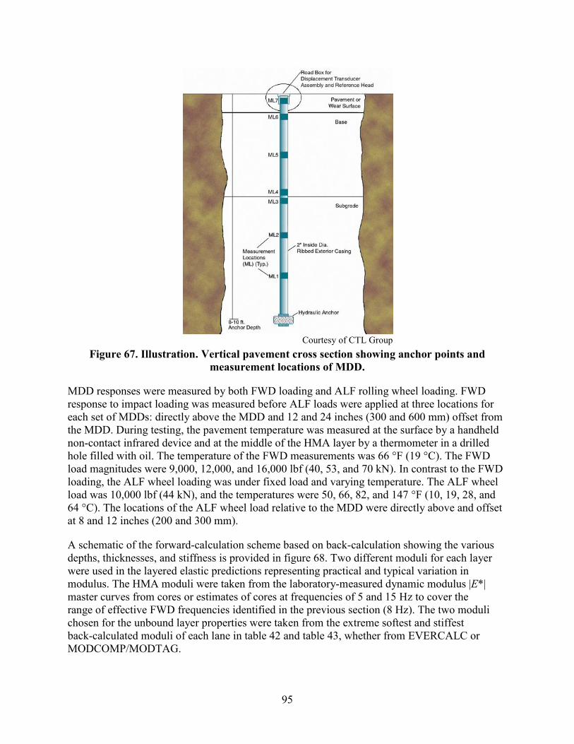
95

Courtesy of CTL Group

Figure 67. Illustration. Vertical pavement cross section showing anchor points and measurement locations of MDD.

MDD responses were measured by both FWD loading and ALF rolling wheel loading. FWD response to impact loading was measured before ALF loads were applied at three locations for each set of MDDs: directly above the MDD and 12 and 24 inches (300 and 600 mm) offset from the MDD. During testing, the pavement temperature was measured at the surface by a handheld non-contact infrared device and at the middle of the HMA layer by a thermometer in a drilled hole filled with oil. The temperature of the FWD measurements was 66 °F (19 °C). The FWD load magnitudes were 9,000, 12,000, and 16,000 lbf (40, 53, and 70 kN). In contrast to the FWD loading, the ALF wheel loading was under fixed load and varying temperature. The ALF wheel load was 10,000 lbf (44 kN), and the temperatures were 50, 66, 82, and 147 °F (10, 19, 28, and 64 °C). The locations of the ALF wheel load relative to the MDD were directly above and offset at 8 and 12 inches (200 and 300 mm).

A schematic of the forward-calculation scheme based on back-calculation showing the various depths, thicknesses, and stiffness is provided in figure 68. Two different moduli for each layer were used in the layered elastic predictions representing practical and typical variation in modulus. The HMA moduli were taken from the laboratory-measured dynamic modulus |E*| master curves from cores or estimates of cores at frequencies of 5 and 15 Hz to cover the range of effective FWD frequencies identified in the previous section (8 Hz). The two moduli chosen for the unbound layer properties were taken from the extreme softest and stiffest back-calculated moduli of each lane in table 42 and table 43, whether from EVERCALC or MODCOMP/MODTAG.

96

°F = 1.8(°C) + 32 1 MPa = 145 psi 1 mm = 0.039 inches

Figure 68. Illustration. Layout of lanes 4 and 11 pavement layer configuration for forward-calculation scheme of MDD instrumentation response.

The measured and predicted MDD deformations from FWD loading are shown in table 44 and table 45 as well as in figure 69 and figure 70. Overall, the two MDD measurements have some variability, but the general trends of smaller deformations deeper in the pavement, farther away from the load, and with smaller loads is captured. The error bars on the predicted MDD deformations represent the standard deviation about the average of the eight different combinations of moduli for the pavement layers used in the predictions. The predicted deformations appear to be less sensitive to modulus than the measured variation in MDD response. The variability in the measured MDD deformations does not appear to be unreasonable given the variability in the back-calculated moduli within and between lanes, as shown in table 42 and table 43.

97

Table 44. MDD peak deflections in mm for lane 4 during FWD loading at 66 °F (19 °C).

Load (kN)

Offset (mm)

Top of CAB Mid of CAB Top of Subgrade

MDD-1 MDD-2

Layered Elastic Predicted

MDD-1 MDD-2

Layered Elastic Predicted

MDD-1 MDD-2

Layered Elastic Predicted

Average Std. Dev. Average

Std. Dev. Average

Std. Dev.

40 0 0.96 0.85 0.79 0.066 0.60 0.44 0.47 0.034 0.42 0.18 0.31 0.022

300 0.55 0.40 0.53 0.042 0.42 0.33 0.39 0.027 0.31 0.23 0.28 0.020 600 0.25 0.23 0.28 0.022 0.22 0.22 0.25 0.018 0.19 0.19 0.21 0.016

53 0 1.31 1.16 1.05 0.088 0.81 0.68 0.63 0.045 0.60 0.43 0.41 0.030

300 0.72 0.44 0.70 0.056 0.59 0.36 0.51 0.036 0.45 0.24 0.37 0.027 600 0.34 0.33 0.37 0.030 0.31 0.32 0.33 0.024 0.27 0.27 0.28 0.021

70 0 1.77 1.33 1.39 0.116 1.16 0.84 0.83 0.059 0.83 0.55 0.55 0.039

300 0.96 0.55 0.93 0.074 0.81 0.45 0.68 0.048 0.62 0.29 0.49 0.035 600 0.46 0.48 0.49 0.039 0.44 0.46 0.44 0.032 0.38 0.40 0.36 0.027

1 kN = 225 lbf 1 mm = 0.039 inches

Table 45. MDD peak deflections in mm for lane 11 during FWD loading at 66 °F (19 °C).

Load (kN)

Offset (mm)

Top of CAB Mid of CAB Top of Subgrade

MDD-1 MDD-2

Layered Elastic Predicted

MDD-1 MDD-2

Layered Elastic Predicted

MDD-1 MDD-2

Layered Elastic Predicted

Average Std. Dev. Average

Std. Dev. Average

Std. Dev.

40 0 0.47 0.38 0.42 0.024 0.33 0.34 0.29 0.012 0.29 0.40 0.22 0.008

300 0.38 0.27 0.32 0.013 0.35 0.26 0.25 0.009 0.28 0.25 0.20 0.007 600 0.18 0.16 0.20 0.006 0.18 0.15 0.18 0.005 0.17 0.16 0.16 0.005

53 0 0.64 0.53 0.56 0.031 0.46 0.48 0.39 0.016 0.38 0.56 0.29 0.010

300 0.48 0.38 0.42 0.017 0.44 0.38 0.34 0.012 0.35 0.36 0.26 0.009 600 0.26 0.22 0.27 0.008 0.25 0.20 0.24 0.007 0.25 0.21 0.21 0.006

70 0 0.87 0.70 0.75 0.042 0.68 0.63 0.52 0.021 0.55 0.74 0.39 0.014

300 0.67 0.52 0.57 0.023 0.60 0.52 0.45 0.016 0.48 0.50 0.35 0.012 600 0.36 0.29 0.36 0.010 0.35 0.28 0.32 0.009 0.34 0.29 0.28 0.008

1 kN = 225 lbf 1 mm = 0.039 inches

98

1 mm = 0.039 inches

Figure 69. Graph. Measured and predicted MDD peak deflection data for lane 4 during FWD loading at 66 °F (19 °C).

00.10.20.30.40.50.60.70.80.9

0 200 400 600

Verti

cal D

efle

ctio

n (m

m)

Transverse Distance (mm)

70 kNTop of SG

0

0.2

0.4

0.6

0.8

1

1.2

1.4

0 200 400 600

Verti

cal D

efle

ctio

n (m

m)

Transverse Distance (mm)

70 kNMid of CAB

00.20.40.60.8

11.21.41.61.8

2

0 200 400 600

Verti

cal D

efle

ctio

n (m

m)

Transverse Distance (mm)

70 kNTop of CAB

0

0.1

0.2

0.3

0.4

0.5

0.6

0.7

0 200 400 600

Verti

cal D

efle

ctio

n (m

m)

Transverse Distance (mm)

53 kNTop of SG

00.10.20.30.40.50.60.70.80.9

0 200 400 600

Verti

cal D

efle

ctio

n (m

m)

Transverse Distance (mm)

53 kNMid of CAB

0

0.2

0.4

0.6

0.8

1

1.2

1.4

0 200 400 600

Verti

cal D

efle

ctio

n (m

m)

Transverse Distance (mm)

53 kNTop of CAB

00.05

0.10.15

0.20.25

0.30.35

0.40.45

0 200 400 600

Verti

cal D

efle

ctio

n (m

m)

Transverse Distance (mm)

40 kNTop of SG

0

0.1

0.2

0.3

0.4

0.5

0.6

0.7

0 200 400 600

Verti

cal D

efle

ctio

n (m

m)

Transverse Distance (mm)

40 kNMid of CAB

0

0.2

0.4

0.6

0.8

1

1.2

0 200 400 600

Verti

cal D

efle

ctio

n (m

m)

Transverse Distance (mm)

Layered Elastic Prediction

Multi Depth Deflectometer

40 kNTop of CAB

99

1 mm = 0.039 inches

Figure 70. Graph. Measured and predicted MDD peak deflection data for lane 11 during FWD loading at 66 °F (19 °C).

00.05

0.10.15

0.20.25

0.30.35

0.40.45

0 200 400 600

Verti

cal D

efle

ctio

n (m

m)

Transverse Distance (mm)

40 kNTop of SG

00.05

0.10.15

0.20.25

0.30.35

0.4

0 200 400 600

Verti

cal D

efle

ctio

n (m

m)

Transverse Distance (mm)

40 kNMid of CAB

00.05

0.10.15

0.20.25

0.30.35

0.40.45

0.5

0 200 400 600

Verti

cal D

efle

ctio

n (m

m)

Transverse Distance (mm)

Layered Elastic Prediction

Multi Depth Deflectometer

40 kNTop of CAB

0

0.1

0.2

0.3

0.4

0.5

0.6

0.7

0 200 400 600

Verti

cal D

efle

ctio

n (m

m)

Transverse Distance (mm)

53 kNTop of CAB

0

0.1

0.2

0.3

0.4

0.5

0.6

0 200 400 600

Verti

cal D

efle

ctio

n (m

m)

Transverse Distance (mm)

53 kNMid of CAB

0

0.1

0.2

0.3

0.4

0.5

0.6

0 200 400 600

Verti

cal D

efle

ctio

n (m

m)

Transverse Distance (mm)

53kNTop of SG

00.10.20.30.40.50.60.70.80.9

1

0 200 400 600

Verti

cal D

efle

ctio

n (m

m)

Transverse Distance (mm)

70 kNTop of CAB

00.10.20.30.40.50.60.70.8

0 200 400 600

Verti

cal D

efle

ctio

n (m

m)

Transverse Distance (mm)

70 kNMid of CAB

00.10.20.30.40.50.60.70.8

0 200 400 600

Verti

cal D

efle

ctio

n (m

m)

Transverse Distance (mm)

70 kNTop of SG

100

In terms of predicted accuracy, the deformations in lane 4 are better overall than in lane 11. The predictions at all depths, offsets, and load levels are within an agreeable range of the measured deformations in lane 11. The far-field response at 23 inches (600 mm) lateral offset is predicted quite well in lanes 4 and 11 at all depths, which suggests that the deeper back-calculated moduli, fixed modulus of the hard bottom, and weather-affected subgrade are reasonable. The deeper deformations toward the center of the load in lane 11 are not predicted as accurately and suggest the pavement structure layer is softer than what was simulated from the back-calculations.

The measured and predicted MDD deformations from ALF wheel loading are shown in table 46 and table 47 as well as in figure 70 through figure 73. Overall, the trends are quite similar to the FWD loading with respect to lane 4 being better predicted than lane 11 and the far-field responses being predicted well. There is less accuracy in the predicted values, and the measured MDD deflections appear to be a bit more erratic than with FWD loading. Based on this analysis, the back-calculated moduli across the ALF sites are reasonable given that the focus of the experiment was in the HMA layers (not the unbound layers) and the vertical deformation at the bottom of the CAB was always captured well.

Table 46. MDD peak deflections in mm for lane 4 during ALF rolling wheel loading at 10,000 lbf (44 kN).

Temp. (°C)

Offset (mm)

Top of CAB Middle of CAB Top of Subgrade

MDD-1 MDD-2

Layered Elastic Predicted

MDD-1 MDD-2

Layered Elastic Predicted

MDD-1 MDD-2

Layered Elastic Predicted

Average Std. Dev. Average

Std. Dev. Average

Std. Dev.

10 0 0.82 0.57 0.76 0.05 0.57 0.37 0.48 0.03 0.44 0.24 0.32 0.02

200 0.59 0.55 0.63 0.05 0.47 0.37 0.44 0.03 0.29 0.28 0.31 0.02 300 0.45 0.49 0.54 0.04 0.41 0.36 0.40 0.03 0.26 0.26 0.29 0.02

19 0 0.87 0.63 0.89 0.07 0.64 0.42 0.53 0.04 0.39 0.27 0.35 0.02

200 0.68 0.56 0.71 0.05 0.45 0.40 0.48 0.03 0.37 0.27 0.33 0.02 300 0.51 0.52 0.59 0.04 0.39 0.38 0.43 0.03 0.31 0.26 0.31 0.02

28 0 0.98 0.90 1.06 0.10 0.73 0.61 0.58 0.04 0.41 0.41 0.37 0.03

200 0.70 0.79 0.80 0.07 0.50 0.56 0.52 0.04 0.40 0.44 0.34 0.03 300 0.53 0.67 0.62 0.05 0.44 0.50 0.46 0.03 0.34 0.39 0.32 0.02

64 0 1.23 1.21 1.92 0.21 0.83 0.82 0.79 0.06 0.52 0.56 0.44 0.03

200 0.86 0.98 1.02 0.10 0.66 0.68 0.65 0.05 0.46 0.50 0.41 0.03 300 0.68 0.73 0.64 0.06 0.55 0.50 0.53 0.04 0.41 0.35 0.37 0.03

°F = 1.8(°C) + 32 1 mm = 0.039 inches

101

Table 47. MDD peak deflections in mm for lane 11 during ALF rolling wheel loading at 10,000 lbf (44 kN).

Temp. (°C)

Offset (mm)

Top of CAB Middle of CAB Top of Subgrade

MDD-1 MDD-2

Layered Elastic Predicted

MDD-1 MDD-2

Layered Elastic Predicted

MDD-1 MDD-2

Layered Elastic Predicted

Average Std. Dev. Average

Std. Dev. Average

Std. Dev.

10 0 0.94 0.51 0.58 0.02 0.65 0.51 0.37 0.01 0.42 0.53 0.26 0.01

200 0.64 0.45 0.48 0.02 0.49 0.45 0.34 0.01 0.39 0.45 0.25 0.01 300 0.36 0.36 0.40 0.01 0.34 0.36 0.31 0.01 0.32 0.35 0.23 0.01

19 0 1.03 0.65 0.67 0.04 0.65 0.62 0.40 0.01 0.42 0.68 0.27 0.01

200 0.64 0.57 0.53 0.02 0.50 0.57 0.36 0.01 0.38 0.58 0.26 0.01 300 0.38 0.43 0.43 0.01 0.37 0.43 0.32 0.01 0.35 0.43 0.24 0.01

28 0 1.24 0.83 0.80 0.05 0.86 0.77 0.44 0.02 0.54 0.89 0.29 0.01

200 0.93 0.69 0.59 0.03 0.75 0.70 0.39 0.01 0.54 0.73 0.27 0.01 300 0.49 0.57 0.45 0.02 0.51 0.58 0.34 0.01 0.40 0.58 0.25 0.01

64 0 2.31 1.84 1.34 0.06 1.68 1.21 0.57 0.02 1.21 1.96 0.35 0.01

200 1.41 1.31 0.71 0.03 1.30 1.03 0.48 0.01 1.25 1.19 0.32 0.01 300 0.53 0.76 0.46 0.01 0.81 0.77 0.39 0.01 0.81 0.63 0.29 0.01

°F = 1.8(°C) + 32 1 mm = 0.039 inches

102

1 mm = 0.039 inches

Figure 71. Graph. Measured and predicted MDD peak deflection data for lane 4 ALF rolling wheel peak deflections at 50 and 66 °F (10 and 19 °C).

00.10.20.30.40.50.60.70.80.9

0 100 200 300Ve

rtica

l Def

lect

ion

(mm

)

Transverse Distance (mm)

Layered Elastic Prediction

Multi Depth Deflectometer

10oCTop of CAB

0

0.1

0.2

0.3

0.4

0.5

0.6

0 100 200 300

Verti

cal D

efle

ctio

n (m

m)

Transverse Distance (mm)

10oCMiddle of CAB

00.05

0.10.15

0.20.25

0.30.35

0.40.45

0.5

0 100 200 300

Verti

cal D

efle

ctio

n (m

m)

Transverse Distance (mm)

10oCTop of SG

0

0.2

0.4

0.6

0.8

1

1.2

0 100 200 300

Verti

cal D

efle

ctio

n (m

m)

Transverse Distance (mm)

Layered Elastic Prediction

Multi Depth Deflectometer

19oCTop of CAB

0

0.1

0.2

0.3

0.4

0.5

0.6

0.7

0 100 200 300

Verti

cal D

efle

ctio

n (m

m)

Transverse Distance (mm)

19oCMid of CAB

00.05

0.10.15

0.20.25

0.30.35

0.40.45

0 100 200 300

Verti

cal D

efle

ctio

n (m

m)

Transverse Distance (mm)

19oCTop of SG

103

1 mm = 0.039 inches

Figure 72. Graph. Measured and predicted MDD peak deflection data for lane 4 ALF rolling wheel peak deflections at 82 and 147 °F (28 and 64 °C).

0

0.2

0.4

0.6

0.8

1

1.2

1.4

0 100 200 300Ve

rtica

l Def

lect

ion

(mm

)

Transverse Distance (mm)

Layered Elastic Prediction

Multi Depth Deflectometer

28oCTop of CAB

00.10.20.30.40.50.60.70.8

0 100 200 300

Verti

cal D

efle

ctio

n (m

m)

Transverse Distance (mm)

28oCMiddle of CAB

00.05

0.10.15

0.20.25

0.30.35

0.40.45

0.5

0 100 200 300

Verti

cal D

efle

ctio

n (m

m)

Transverse Distance (mm)

28oCTop of SG

0

0.5

1

1.5

2

2.5

0 100 200 300

Verti

cal D

efle

ctio

n (m

m)

Transverse Distance (mm)

Layered Elastic Prediction

Multi Depth Deflectometer

64oCTop of CAB

0

0.2

0.4

0.6

0.8

1

1.2

0 100 200 300

Verti

cal D

efle

ctio

n (m

m)

Transverse Distance (mm)

64oCMidle of CAB

0

0.1

0.2

0.3

0.4

0.5

0.6

0.7

0 100 200 300

Verti

cal D

efle

ctio

n (m

m)

Transverse Distance (mm)

64oCTop of SG

104

1 mm = 0.039 inches

Figure 73. Graph. Measured and predicted MDD peak deflection data for lane 11 ALF rolling wheel peak deflections at 50 and 66 °F (10 and 19 °C).

00.10.20.30.40.50.60.70.80.9

1

0 100 200 300Ve

rtica

l Def

lect

ion

(mm

)

Transverse Distance (mm)

Layered Elastic Prediction

Multi Depth Deflectometer

10oCTop of CAB

0

0.1

0.2

0.3

0.4

0.5

0.6

0.7

0 100 200 300

Verti

cal D

efle

ctio

n (m

m)

Transverse Distance (mm)

10oCMiddle of CAB

0

0.1

0.2

0.3

0.4

0.5

0.6

0 100 200 300

Verti

cal D

efle

ctio

n (m

m)

Transverse Distance (mm)

10oCTop of SG

0

0.2

0.4

0.6

0.8

1

1.2

0 100 200 300

Verti

cal D

efle

ctio

n (m

m)

Transverse Distance (mm)

Layered Elastic Prediction

Multi Depth Deflectometer

19oCTop of CAB

0

0.1

0.2

0.3

0.4

0.5

0.6

0.7

0 100 200 300

Verti

cal D

efle

ctio

n (m

m)

Transverse Distance (mm)

19oCMid of CAB

00.10.20.30.40.50.60.70.8

0 100 200 300

Verti

cal D

efle

ctio

n (m

m)

Transverse Distance (mm)

19oCTop of SG

105

1 mm = 0.039 inches Figure 74. Graph. Measured and predicted MDD peak deflection data for lane 11 ALF

rolling wheel peak deflections at 82 and 147 °F (28 and 64 °C).

Seasonal Monitoring of Pavement Sections with FWD

Lanes 4 and 11 were monitored over 26 months as part of a focused seasonal monitoring program using only FWD loading. At least one test per month was conducted, and, at times, a separate test was carried out before or after heavy rainstorms or periods of wet weather. The data were analyzed to determine the sensor offset location that indicated there was little to no change in deflection regardless of the season or weather characteristics. The variation in deflection throughout the year was evident at the sensor at 24 inches (61 cm), while the sensor at 36 inches (91 cm) was essentially unaffected. This indicates that the depth to a saturated subgrade that can be said to be unaffected by weather was shallower than assumed.

DIRECT MEASUREMENT OF ASPHALT LAYER MODULUS

IDT Resilient Modulus of Asphalt

As described in the previous section, resilient modulus of the HMA mixtures was measured in IDT. Plant-produced mixture sampled during construction was compacted to 7 percent air voids

0

0.2

0.4

0.6

0.8

1

1.2

1.4

0 100 200 300Ve

rtica

l Def

lect

ion

(mm

)

Transverse Distance (mm)

Layered Elastic Prediction

Multi Depth Deflectometer

28oCTop of CAB

00.10.20.30.40.50.60.70.80.9

1

0 100 200 300

Verti

cal D

efle

ctio

n (m

m)

Transverse Distance (mm)

28oCMiddle of CAB

00.10.20.30.40.50.60.70.80.9

1

0 100 200 300

Verti

cal D

efle

ctio

n (m

m)

Transverse Distance (mm)

28oCTop of SG

0

0.5

1

1.5

2

2.5

0 100 200 300

Verti

cal D

efle

ctio

n (m

m)

Transverse Distance (mm)

Layered Elastic Prediction

Multi Depth Deflectometer

64oCTop of CAB

00.20.40.60.8

11.21.41.61.8

0 100 200 300

Verti

cal D

efle

ctio

n (m

m)

Transverse Distance (mm)

64oCMidle of CAB

0

0.5

1

1.5

2

2.5

0 100 200 300Ve

rtica

l Def

lect

ion

(mm

)Transverse Distance (mm)

64oCTop of SG

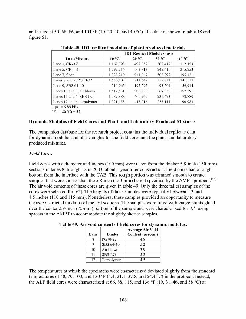
106

and tested at 50, 68, 86, and 104 °F (10, 20, 30, and 40 °C). Results are shown in table 48 and figure 61.

Table 48. IDT resilient modulus of plant produced material.

Lane/Mixture IDT Resilient Modulus (psi)

10 °C 20 °C 30 °C 40 °C Lane 1, CR-AZ 1,167,298 498,752 305,418 112,158 Lane 5, CR-TB 1,292,216 562,813 245,616 215,253 Lane 7, fiber 1,928,210 944,047 506,297 195,421 Lanes 8 and 2, PG70-22 1,656,403 811,647 355,733 241,517 Lane 9, SBS 64-40 516,065 197,292 93,501 59,914 Lanes 10 and 3, air blown 1,517,831 902,838 269,850 157,291 Lanes 11 and 4, SBS-LG 1,087,988 460,965 231,473 78,880 Lanes 12 and 6, terpolymer 1,021,153 418,016 237,114 90,983

1 psi = 6.89 kPa °F = 1.8(°C) + 32

Dynamic Modulus of Field Cores and Plant- and Laboratory-Produced Mixtures

The companion database for the research project contains the individual replicate data for dynamic modulus and phase angles for the field cores and the plant- and laboratory- produced mixtures.

Field Cores

Field cores with a diameter of 4 inches (100 mm) were taken from the thicker 5.8-inch (150-mm) sections in lanes 8 through 12 in 2003, about 1 year after construction. Field cores had a rough bottom from the interface with the CAB. This rough portion was trimmed smooth to create samples that were shorter than the 5.8-inch (150-mm) height specified by the AMPT protocol.(56) The air void contents of these cores are given in table 49. Only the three tallest samples of the cores were selected for |E*|. The heights of those samples were typically between 4.3 and 4.5 inches (110 and 115 mm). Nonetheless, these samples provided an opportunity to measure the as-constructed modulus of the test sections. The samples were fitted with gauge points glued over the center 2.9-inch (75-mm) portion of the sample and were characterized for |E*| using spacers in the AMPT to accommodate the slightly shorter samples.

Table 49. Air void content of field cores for dynamic modulus.

Lane Binder Average Air Void Content (percent)

8 PG70-22 4.8 9 SBS 64-40 5.2

10 Air blown 3.9 11 SBS-LG 5.2 12 Terpolymer 4.5

The temperatures at which the specimens were characterized deviated slightly from the standard temperatures of 40, 70, 100, and 130 °F (4.4, 21.1, 37.8, and 54.4 °C) in the protocol. Instead, the ALF field cores were characterized at 66, 88, 115, and 136 °F (19, 31, 46, and 58 °C) at

107

frequencies of 0.1, 0.5, 1, 5, 10, and 20 Hz. The low-temperature features of the AMPT were malfunctioning at the time the data were collected. The dynamic modulus |E*| master curves of the field cores are shown in figure 75 in log-log scale to highlight the variation in the low modulus region and in figure 76 in semilog scale to highlight the variation in the stiffer moduli. Only the range of measured values is shown; the master curves are not extrapolated in any way. Several observations can be made regarding the stiffness variation with temperature and frequency of the mixtures in their field density conditions.

1 MPa = 145 psi

Figure 75. Graph. |E*| dynamic modulus for field cores versus reduced frequency in log-log scale.

10

100

1000

10000

0.00001 0.0001 0.001 0.01 0.1 1 10 100

Reduced Frequency (Hz)

Dyn

amic

Mod

ulus

(MPa

)

Lane 8, ControlLane 9, SBS 64-40Lane 10, Air BlownLane 11, SBS-LGLane 12, Terpolymer

108

1 MPa = 145 psi

Figure 76. Graph. |E*| dynamic modulus for field cores versus reduced frequency in semilog scale.

In the extreme high-temperature low-frequency region where rutting was primarily induced, the lane 12 terpolymer and lane 9 SBS 64-40 mixtures had the lowest and similar stiffness. Lane 9 (SBS 64-40) had the overall lowest stiffness of all mixtures. The lane 8 PG70-22 and lane 11 SBS-LG mixtures had the next highest stiffness in the high-temperature low-frequency region of the master curve. The stiffest mixture in the extreme high-temperature low-frequency region of the master curve is the lane 10 air-blown mixture.

In the intermediate 66 °F (19 °C) temperature region, which is shown in the right portion of the curves in figure 75 and figure 76, the stiffest mixture was found in lane 8 (PG70-22) followed closely by lane 10 (air blown). The softest mixture was found in lane 9 (SBS 64-40). Lane 12 (terpolymer) and lane 11 (SBS-LG) were similar and had a stiffness between the extremes.

Plant-Produced Mixtures

Loose mixture was sampled in pails during construction and compacted to a target density of 7 percent. The average air void content of the specimens tested is shown in table 50. The lane 7 fiber and lane 1 CR-AZ mixtures were not tested. The plant-produced mixtures were tested at the same temperatures and frequencies at which the field cores were tested: 66, 88, 115, and 136 °F (19, 31, 46, and 58 °C) at frequencies of 0.1, 0.5, 1, 5, 10, and 20 Hz. The low-temperature features of the AMPT were malfunctioning at the time the data were collected. The dynamic modulus |E*| master curves of the plant-produced mixtures are shown in figure 77 in log scale to highlight the variation in the low modulus region and in figure 78 in semilog scale to highlight the variation in the stiffer moduli. Only the range of measured values is shown; the master curves are not extrapolated in any way.

0

1000

2000

3000

4000

5000

6000

7000

8000

0.00001 0.0001 0.001 0.01 0.1 1 10 100

Reduced Frequency (Hz)

Dyn

amic

Mod

ulus

(MPa

)

Lane 8, ControlLane 9, SBS 64-40Lane 10, Air BlownLane 11, SBS-LGLane 12, Terpolymer

109

Table 50. Air void content of plant-produced mixture for dynamic modulus.

Lane Binder Average Air Void Content (percent)

2 and 8 PG70-22 6.8 3 and 10 Air blown 6.2 4 and 11 SBS-LG 6.8 5 CR-TB 7.0 6 and 12 Terpolymer 6.0 9 SBS 64-40 6.5

1 MPa = 145 psi

Figure 77. Graph. |E*| dynamic modulus for plant-produced mixtures versus reduced frequency in log-log scale.

10

100

1000

10000

0.00001 0.0001 0.001 0.01 0.1 1 10 100

Reduced Frequency (Hz)

Dyn

amic

Mod

ulus

(MPa

)

Lane 2 & 8, ControlLane 3 & 10, Air BlownLane 4 & 11, SBS-LGLane 5, CR-TBLane 6 & 12, TerpolymerLane 9, SBS 64-40

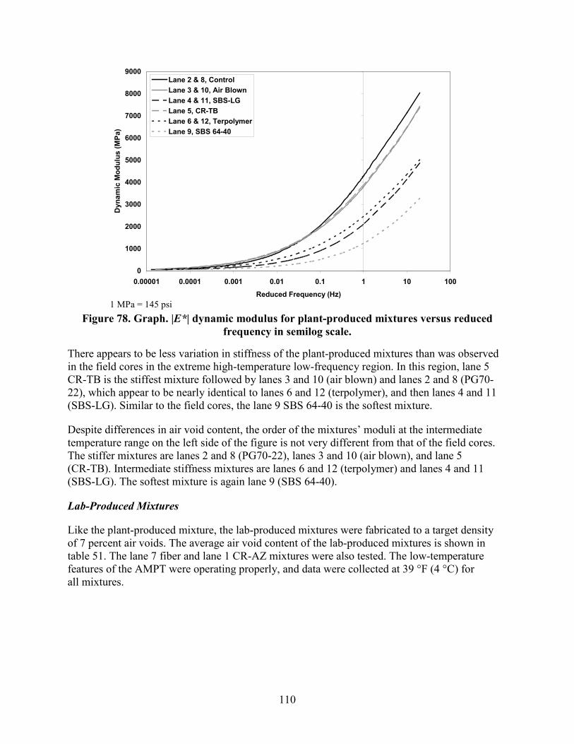
110

1 MPa = 145 psi

Figure 78. Graph. |E*| dynamic modulus for plant-produced mixtures versus reduced frequency in semilog scale.

There appears to be less variation in stiffness of the plant-produced mixtures than was observed in the field cores in the extreme high-temperature low-frequency region. In this region, lane 5 CR-TB is the stiffest mixture followed by lanes 3 and 10 (air blown) and lanes 2 and 8 (PG70-22), which appear to be nearly identical to lanes 6 and 12 (terpolymer), and then lanes 4 and 11 (SBS-LG). Similar to the field cores, the lane 9 SBS 64-40 is the softest mixture.

Despite differences in air void content, the order of the mixtures’ moduli at the intermediate temperature range on the left side of the figure is not very different from that of the field cores. The stiffer mixtures are lanes 2 and 8 (PG70-22), lanes 3 and 10 (air blown), and lane 5 (CR-TB). Intermediate stiffness mixtures are lanes 6 and 12 (terpolymer) and lanes 4 and 11 (SBS-LG). The softest mixture is again lane 9 (SBS 64-40).

Lab-Produced Mixtures

Like the plant-produced mixture, the lab-produced mixtures were fabricated to a target density of 7 percent air voids. The average air void content of the lab-produced mixtures is shown in table 51. The lane 7 fiber and lane 1 CR-AZ mixtures were also tested. The low-temperature features of the AMPT were operating properly, and data were collected at 39 °F (4 °C) for all mixtures.

0

1000

2000

3000

4000

5000

6000

7000

8000

9000

0.00001 0.0001 0.001 0.01 0.1 1 10 100

Reduced Frequency (Hz)

Dyn

amic

Mod

ulus

(MPa

)

Lane 2 & 8, ControlLane 3 & 10, Air BlownLane 4 & 11, SBS-LGLane 5, CR-TBLane 6 & 12, TerpolymerLane 9, SBS 64-40

111

Table 51. Air void content of lab-produced mixture for dynamic modulus.

Lane Binder Average Air Void Content (percent)

1 top CR-AZ — 2 and 8 PG70-22 7.0 3 and 10 Air blown 6.8 4 and 11 SBS-LG 7.1 5 CR-TB 6.7 6 and 12 Terpolymer 6.7 7 Fiber — 9 SBS 64-40 7.4

— Indicates the mixture was not lab produced for this experiment.

Figure 79 and figure 80 show the lab-produced dynamic modulus master curves in log-log and semilog scale, respectively. The two stiffest mixtures in the low-frequency high-temperature range of the master curve at the left side are air blown and CR-TB. The two softest mixtures were SBS 64-40 and CR-AZ. Intermediate stiffness mixtures in the high-temperature low-frequency region were terpolymer, PG70-22, SBS-LG, and fiber. The logarithmic scale emphasizes differences between the mixtures, but their moduli were not extremely different in this range.

1 MPa = 145 psi

Figure 79. Graph. |E*| dynamic modulus for lab-produced mixtures versus reduced frequency in log-log scale.

10

100

1000

10000

100000

0.00001 0.0001 0.001 0.01 0.1 1 10 100 1000 10000

Reduced Frequency (Hz)

Dyn

amic

Mod

ulus

(MPa

)

ControlAir BlownCR-TBFiberSBS 64-40SBS LGCR-AZTerpolymer

112

1 MPa = 145 psi

Figure 80. Graph. |E*| dynamic modulus for lab-produced mixtures versus reduced frequency in semilog scale.

In the intermediate- and low-temperature high-frequency range, the mixtures are more different from one another, as seen more clearly in semilog scale. There are distinct clusters of mixtures where the PG70-22 binder, fiber, and air blown are stiffest. The softest mixture is SBS 64-40. The remaining mixtures, CR-AZ, CR-TB, SBS-LG, and terpolymer, all have similar stiffness.

The phase angle master curves from the dynamic modulus tests for the lab-produced mixtures are shown in figure 81. At the left side of the curve in the high-temperature low-frequency region, the mixtures with the more elastic or lowest phase angles are SBS 64-40, SBS-LG, and terpolymer while the mixtures with the more viscous or highest phase angles are PG70-22, fiber, CR-TB, CR-AZ, and air blown.

0

2000

4000

6000

8000

10000

12000

14000

16000

18000

0.00001 0.0001 0.001 0.01 0.1 1 10 100 1000 10000

Reduced Frequency (Hz)

Dyn

amic

Mod

ulus

(MPa

)

ControlAir BlownCR-TBFiberSBS 64-40SBS LGCR-AZTerpolymer

113

Figure 81. Graph. Curves fit to phase angle measured during dynamic modulus test versus

reduced frequency.

The plant-produced laboratory-compacted dynamic modulus and laboratory-batched dynamic modulus are comparable for the PG70-22, air-blown, and SBS-LG mixtures, whereas the plant-produced SBS 64-40, terpolymer, and CR-TB mixtures are stiffer than lab-batched. Cores from the 5.8-inch (150-mm) lane 8 PG70-22 and lane 9 SBS 64-40 sections were stiffer than lab-batched materials but were also more dense. The 5.8-inch (150-mm) lane 10 air-blown cores were less stiff than the lab-produced samples, which were more dense than the cores. Cores from the 5.8-inch (150-mm) lane 11 SBS-LG and lane 12 terpolymer sections exhibited comparable stiffness to the lab-batched materials, but the cores were also more dense.

MEPDG AND STANDALONE ANALYSES OF ALF PAVEMENTS

Several unintended consequences of various features within the MEPDG software would not allow the most faithful simulation of the ALF loading. A surrogate for the MEPDG was utilized that enabled features implemented within the MEPDG to be adjusted or turned off completely. Although it would have been desirable to use the MEPDG specifically, a standalone version of the MEPDG developed by Thyagarajan et al. was implemented within Microsoft Excel®.(57) The MEPDG standalone software was developed to conduct independent analyses for comparison with MEPDG predictions for the purpose of analyzing the consequences of assuming constant tire pressure and constant tire contact area in the MEPDG for strain computations. The software was validated to ensure the predictions of the MEPDG without any chosen adjustments could be reproduced. An example of valid reproduction of the MEPDG is shown in figure 82.(57)

0

5

10

15

20

25

30

35

40

0.00001 0.0001 0.001 0.01 0.1 1 10 100 1000 10000

Reduced Frequency (Hz)

Phas

e A

ngle

(deg

rees

)

ControlAir BlownCR-TBFiberSBS 64-40SBS LGCR-AZTerpolymer

114

1 inch = 25.4 mm

Figure 82. Graph. Rut depth versus pavement age from MEPDG and standalone application.

ALF Wheel and Tire

The MEPDG offers a special axle configuration option for users to customize and define the number of contact areas, the size of contact area, the wheel load, and the inflation pressure. Pressure is uniform and circular in shape. The ALF’s 425 super-single tire was simulated using the custom axle configuration for rutting with a wheel load of 10,000 lbf (44 kN) and tire inflation pressure of 100 psi (689 kPa). Fatigue loading utilized 16,000 lbf (71 kN) wheel load and 120 psi (827 kPa) inflation pressure.

Wheel wander can also be prescribed with the custom axle configuration by specifying the standard deviation of an ideal normal Gaussian distribution of wheel wander. Zero wheel wander was input for rutting, and the same standard deviation of 5.25 inches (133 mm) programmed into the ALF mechanical loading was used for fatigue.

Another caveat of the special axle configuration wheel loading is that the number of passes per month of the special axle must be input. However, many times, the ALF loading was completed within a month. Naturally, this creates scenarios where there would be very few output data points when ALF loading was simulated faithfully. Instead, approximately 58 data points, or 58 months, were assumed to provide sufficient resolution for all predicted distresses. Therefore, fatigue was programmed to have 5,208 passes per month over 58 months for a total of 302,064 passes. Rutting was programmed to have 700 passes per month over 58 months for a total of 40,600 passes.

A final caveat associated with the custom axle configuration option is that a representative frequency must be specified for all depths. The speed of the tire induces a stress pulse that is distributed within the pavement structure. The net effect is that effective load time gets longer with depth; that is, frequency of the load become smaller with depth. This feature within the normal load spectra portion of the MEPDG appears not to have been implemented in the custom axle configuration option. A frequency of 10 Hz was arbitrarily chosen as representative for all depths for the ALF wheel speed of 11 mi/h (18 km/h). This was considered conservative given an analysis of the ALF tire and speed using the empirical Odemark technique within the MEPDG that determined effective load pulse time and frequency at the top surface to be 18 Hz and the frequency at the bottom of the HMA layers to be 9.1 and 7.3 Hz for 4- and 5.8-inch (100- and 150-mm) sections, respectively, using HMA moduli typical for rutting.(1) When wheel load and moduli typical for fatigue were used in the Odemark technique, the frequency at the top surface

115

was 15 Hz, but the frequency at the bottom of the HMA layers was found to be 4.2 and 3.1 Hz for 4- and 5.8-inch (100- and 150-mm) sections, respectively.

ALF Temperature and Aging

The MEPDG was developed to analyze pavement designs over a realistic lifetime and therefore considers seasonal and daily variations in temperature and moisture. The Enhanced Integrated Climatic Model (EICM) supplies the MEPDG with an input file that contains a complex statistical record of temperature variations throughout the depth of the pavement at various times of day, month, and year. This feature is then used to adjust the moduli of various pavement layers to simulate seasonal effects on pavement mechanics.

The controlled temperatures of the ALF challenged the EICM feature of the MEPDG. Controlled temperatures were simulated by formatting an EICM text input file that forced temperature at all depths and all times of the year to be constant. However, the consequence of the forced temperature for rutting within the MEPDG was that higher temperatures applied over the programmed 58 months artificially stimulated the Global Aging System Model in the MEPDG to increase the stiffness of the HMA layers over time to emulate oxidative aging and hardening. Figure 83 shows an example of this increase in stiffness of the HMA layer from one of the early runs of the MEPDG.

1 psi = 6.89 kPa Figure 83. Graph. Asphalt modulus versus pavement age from early run of MEPDG.

Circumventing and eliminating this excessive stiffening behavior within the framework of the MEPDG was attempted by inputting binder viscosity temperature susceptibility parameters, which govern age hardening and have a very low slope. This was unsuccessful and produced erroneous results. The standalone MEPDG surrogate in Microsoft Excel® allowed the stiffening of the modulus with time caused by the Global Aging System Model to be turned off.

0

20,000

40,000

60,000

80,000

100,000

120,000

140,000

160,000

180,000

200,000

0 6 12 18 24 30 36 42 48 54 60

Pavement Age (month)

Mod

ulus

(psi

)

AC1(1) h=0.5AC1(2) h=0.5AC1(3) h=1.0AC1(4) h=1.0AC1(5) h=1.0

116

Other Caveats of the MEPDG and Standalone

To validate the standalone application for ALF conditions, the distresses predicted over the design period in site 1 (147 °F (64 °C) rutting at 10,000 lbf (44 kN)) of lane 2 were compared with the values predicted by the MEPDG. The aged modulus computed by the MEPDG over the period was used in the standalone application. The bottom-up fatigue cracking and HMA rutting predicted by both the MEPDG and the standalone application compared well. For efficiency in all other sites and lanes, the distress predicted by the standalone application at the first month of the design period was compared with the MEPDG predictions. In the first month, both the MEPDG and standalone analyses used the same HMA modulus.

The distresses (both HMA rutting and bottom-up fatigue cracking) predicted by the standalone application in the first month in site 1 (147 °F (64 °C) rutting at 10,000 lbf (44 kN)) and site 2 (165 °F (74 °C) rutting at 10,000 lbf (44 kN)) of all the lanes compared well with the MEPDG predictions. In site 3 (66 °F (19 °C) fatigue at 16,000 lbf (71 kN)) of all the lanes, the HMA rutting predicted by the standalone application in the first month was higher than the MEPDG predictions. However, the bottom-up fatigue cracking predicted by both analyses matched well. The possible reason behind this may be the heavy load used in site 3. For the given tire inflation pressure (120 psi (827 kPa)), the heavy load corresponds to wider tire contact area. The particular implementation of the layered elastic analysis program JULEA used in MEPDG analyses has some difficulties computing the strain levels in the top of the HMA layer under these conditions. This is not to say JULEA is incorrect, rather, what was computed from the output was likely incorrect. The MEPDG extrapolates the strain computed at the surface and at the depth of 0.148 inches (3.76 mm) multiplied by the contact radius to compute strain levels within this region. The strain computed in this region corresponds to a tensile strain instead of compression that causes rutting. The HMA rutting model has a depth correction factor kz which is mostly negative for the top HMA layer (0.5 inches (13 mm) thick). The standalone application computes the HMA rutting when the product of the correction factor and the strain response is positive. This prevents numerical error while solving the HMA rutting model. The heavy load in site 3 increased the compressive strain at the top sublayer, and, along with the negative correction factor, this resulted in high rutting at the top sublayer. This might be the reason for the high rutting predicted by the standalone application when compared to the MEPDG predictions. The possible solution to this was to change the rutting computation procedure in the standalone application, which may result in no rutting in the top sublayer. Of course, this is only an issue when rutting in the 66 °F (19 °C) fatigue sections is compared and evaluated.

HMA Dynamic Modulus Input to MEPDG

Reflecting As-Built HMA Layer Conditions with Dynamic Modulus |E*| Input

Construction data in chapter 2 showed all 12 ALF lanes were not constructed with identical density. The thinner 4-inch (100-mm) sections in lanes 1–7 were compacted to a slightly less dense state than the mixtures in the thicker 5.8-inch (150-mm) sections in lanes 8–12. Also, there was variation in density within the 4- and 5.8-inch (100- and 150-mm) sections.

Ideally, the in situ material for all 12 lanes would be directly characterized for dynamic modulus |E*| and input into the MEPDG. This was possible for lanes 8–12, as discussed in the previous section. Advantages to this approach are that the effect of field compaction is directly taken into

117

consideration and that it accounts for HMA plant production rather than ideal laboratory batching and compaction (see lime nugget distribution in chapter 2). A number of researchers have found gyratory-compacted HMA mixtures exhibit stiffer and stronger material properties than field compaction. (See references 58–62.) However, the nominal 4-inch (100-mm) thickness of lanes 1–7 prevented cores taken from the ALF pavements to be reasonably characterized in standard |E*| protocols.

The as-built HMA dynamic modulus |E*| input for the 4-inch (100-mm) lanes was estimated as follows. For lane 2 (PG70-22), lane 3 (air blown), lane 4 (SBS-LG), and lane 6 (terpolymer), the difference in air void content between 5.8-inch (150-mm) field cores and the density of the mixture of interest in the 4-inch (100-mm) test section was determined. Then, a density correction factor was used to adjust the known modulus at a given air void content to a softer or stiffer modulus at a slightly different air void content. For lane 5 (CR-TB), the difference in air void content between the lab-compacted plant-produced materials and the density of the test lane was determined. Then, the correction factor was applied to adjust the stiffness of the lab sample to the field conditions. Modulus alone cannot explain the notably better cracking performance of lane 1 (CR-AZ) and lane 7 (fiber) compared to the other mixtures in the 4-inch (100-mm) sections. In addition, the less modest dynamic modulus |E*| of the gap-graded CR-AZ mixture is more likely a reflection of the tests being ran without confinement as well as different volumetric properties compared to the other dense graded mixtures. The repeated load permanent deformation flow number test did use confinement.

A density correction factor for HMA dynamic modulus used in the described procedure was generated using the Witczak and Hirsch predictive equations for dynamic modulus.(1,63) The variations in air void content, VMA, and VFA properties of the HMA mixtures from construction data were collected as inputs to the two predictive equations. A reference condition of 5 percent air voids was chosen. The predicted moduli from the equations for a wide range of binder viscosity input for the Witczak model and binder |G*| input for the Hirsch model were used to generate the ratio of modulus across all temperatures. It was observed that for every 1 percent increase or decrease in air void content there was a corresponding 5.69 percent decrease or increase in stiffness. The slope of the fit line in figure 84 is 0.0569.

118

Figure 84. Graph. Ratio between predicted dynamic modulus at various air void contents

relative to a reference condition.

MEPDG |E*| Input Formatting

The MEPDG can import measured |E*| dynamic modulus at temperatures and frequencies determined by the user. The MEPDG then conducts the time and temperature shifting and assembles dynamic modulus master curves. However, the MEPDG requires dynamic modulus at temperatures equal or colder than 14 °F (-10 °C). Also, the MEPDG cannot accept moduli softer than 10,000 psi (69 MPa) (very high temperatures and low frequencies). The raw data and master curves shown in figure 75 through figure 80 did not have data at temperatures as cold as required by the MEPDG and contained isolated moduli that were softer than 10,000 psi (69 MPa). The low-temperature data were synthesized by fitting a Hirsch predictive model for dynamic modulus using the volumetric properties of the mixtures and measured binder |G*| dynamic shear moduli. Very low-temperature dynamic moduli were calculated assuming limiting binder moduli of 290,000 psi (2 GPa). Predicted dynamic moduli at 10 °F (-12 °C) were input along with the measured |E*| data into the MEPDG. An example of the extrapolation and limiting low modulus is shown in figure 85.

0.75

0.8

0.85

0.9

0.95

1

1.05

1.1

3 4 5 6 7 8 9 10

Air Void Content (%)

Dyn

amic

Mod

ulus

Rat

io |E

*|

Witczak ModelHirsch ModelCorrection Factor, 0.056 slope

119

1 MPa = 145 psi

Figure 85. Graph. Extrapolated dynamic modulus in log scale versus reduced frequency.

The combined measured and low-temperature extrapolated |E*| dynamic moduli were assembled and imported into the MEPDG for temperature scenarios of 66, 113, 147, and 165 °F (19, 45, 64, and 74 °C). Then, the moduli from the first month of the MEPDG was selected and input to the standalone application for a fixed modulus that does not age and stiffen with time. These moduli for the HMA layers are summarized in table 52. Although the temperature was designed to be fixed with depth and time using modified input files from the EICM, moduli from the MEPDG did vary slightly with depth. The moduli reported in table 52 are the average of all sublayers in the HMA. The typical variation of moduli from top to bottom was 6 percent for the 4-inch (100-mm) lanes at 147 and 165 °F (64 and 74 °C), 16 percent for the 4-inch (100-mm) lanes at 66 °F (19 °C), 9 percent for the 5.8-inch (150-mm) lanes at 147 °F (64 °C), 17 percent for the 5.8-inch (150-mm) lanes at 113 °F (45 °C), and 17 percent for the 5.8-inch (150-mm) lanes at 66 °F (19 °C).

1

10

100

1000

10000

100000

1.E-08 1.E-06 1.E-04 1.E-02 1.E+00 1.E+02 1.E+04 1.E+06 1.E+08

Reduced Freq. (Hz)

|E*|

(MP

a)

Average, |E*| MpaSigmoid Fit, |E*| MpaMEPDG Extrapolation Example"Clipped"

120

Table 52. First-month modulus from MEPDG used in standalone program.

Lane Site Temperature

(°C) As-Built HMA Modulus (psi)

As-Designed HMA Modulus (psi)

2; PG70-22 1 64 25,294 42,099 2 74 14,596 22,379 3 19 1,019,332 1,235,002

3; air blown 1 64 35,633 54,837 2 74 20,229 30,687 3 19 811,735 947,703

4; SBS-LG 1 64 23,070 26,881 2 74 14,315 17,035 3 19 716,739 711,956

5; CR-TB 1 64 50,716 37,358 2 74 27,040 21,552 3 19 855,027 718,840

6; terpolymer 1 64 17,579 21,721 2 74 11,764 14,822 3 19 647,964 654,057

8; PG70-22 1 64 26,684 41,723 2 45 117,266 176,840 3 19 1,078,588 1,225,775

9; SBS 64-40 1 64 17,643 16,314 3 19 371,394 298,872

10; air blown 1 64 40,874 54,427 2 45 146,546 182,274 3 19 925,573 941,817

11; SBS-LG 1 64 25,200 26,682 2 45 91,866 88,306 3 19 780,127 703,421

12; terpolymer 1 64 20,107 21,541 2 45 74,043 67,062 3 19 744,576 640,028

°F = 1.8(°C) + 32 1 psi = 6.89 kPa

It was recognized that high-temperature ALF rutting at 147 and 165 °F (64 and 74 °C) was predicted with MEPDG models using dynamic modulus master curves that were generated from physical test data where the highest temperature was only 136 °F (58 °C). This created some concern that material properties were being extrapolated beyond the range of what was physically measured. However, time-temperature superposition was used to create the dynamic modulus master curves. Time-temperature superposition allows temperature effects and rate effects (time, frequency) to be interchanged. In other words, the dynamic modulus at a cooler temperature and given frequency is equivalent to the dynamic modulus at a warmer temperature and higher frequency; temperature and rate effects are inversely related. Table 53 shows an example of the dynamic modulus master curve data from the high-temperature portion of the control lab-produced mixture. The non-reduced frequencies and corresponding temperatures are provided in the left portion of the table and correspond to the individual reduced frequencies (at a 66 °F (19 °C) reference temperature) and dynamic modulus counterpart in the right side of the table. The nearest equivalent dynamic modulus from temperatures and frequencies of 147 °F (64 °C) at 10 Hz and 165 °F (74 °C) at 10 Hz are equivalently the dynamic modulus at 136 °F (58 °C) at frequencies near 5 and 1 Hz, respectively. The equivalent computed frequencies at

121

136 °F (58 °C) are 3.4 and 0.65 Hz for identical modulus at 147 °F (64 °C) at 10 Hz and 165 °F (74 °C), respectively.

Table 53. Example of equivalent |E*| temperatures and frequencies using time-temperature superposition.

Temperature (°C)

Frequency (Hz)

Reduced Frequency (Hz)

|E*| MPa psi

58 20 3.09E-03 492 71,323 58 10 1.55E-03 360 52,157 64 20 1.06E-03 303 43,906 58 5 7.73E-04 263 38,179 64 10 5.28E-04 222 32,205 64 5 2.64E-04 164 23,774 74 20 2.07E-04 148 21,424 58 1 1.55E-04 131 18,932 74 10 1.04E-04 111 16,030 58 0.5 7.73E-05 98 14,240 64 1 5.28E-05 84 12,244 74 5 5.18E-05 84 12,153 64 0.5 2.64E-05 65 9,420 58 0.1 1.55E-05 54 7,784 74 1 1.04E-05 47 6,791 64 0.1 5.28E-06 38 5,474

74* 0.5* 5.18E-06* 38* 5,442* 74* 0.1* 1.04E-06* 24* 3,489*

°F = 1.8(°C) + 32 *Extrapolation beyond laboratory measured conditions.

Quantifying Cracking

Predicted cracking quantified by the MEPDG and measured under the ALF are different in nature. ALF measures percent cracking within the boundary of the area loaded by the single tire. With wheel wander, the dimensions of the ALF loaded area were 3.7 by 33 ft (1.13 by 10.05 m), equaling 122.6 ft2 (11.4 m2). The percent ALF cracking is calculated using figure 86.

Figure 86. Equation. ALF cracking.

The equivalent MEPDG cracking for the same amount of ALF cracking can be calculated assuming two loaded areas within a standard lane width of 12 ft (3.66 m), as shown in figure 87.

Figure 87. Equation. Equivalent MEPDG cracking.

A factor of 0.31 is used to adjust the ALF cracking to what is comparable with MEPDG. It is calculated by dividing the two reference areas, 122.6 ft2 (11.4 m2) divided by 120.7 ft2 (36.8 m2).

122

PRIMARY STRAIN RESPONSE OF PAVEMENTS

Strain gauges were installed in one of the four sites of each lane. Figure 88 is schematic of the strain gauge layout and orientation. An evaluation of the measured strain gauge response against that predicted by the linearly elastic mechanistic material properties provides a qualitative assessment of those assigned linear elastic properties. It must be recognized that the strain gauge measured responses cannot be taken as true since the presence of the gauge embedded within the HMA layer and circumstances of installation and orientation can affect the response. However, strain gauges can provide reality checks on the layered elastic mechanistic pavement models and chosen material property inputs.

1 ft = 0.305 m 1 inch = 25.4 mm

Figure 88. Illustration. Layout of an ALF test site with strain gauges.

Strain gauge responses were measured before any fatigue or rutting loading began. HMA tensile strains were measured under a variety of temperatures, wheel loads, and transverse wheel offsets. The series of tests that was closest to the ALF fatigue loading conditions and corresponding MEPDG standalone output (66 °F (19 °C) and 16,000 lbf (70 kN)) were strain measurements controlled at 66 °F (19 °C) at 14,500 lbf (64 kN). Figure 89 and table 54 compare the measured HMA tensile strains against layered elastic MEPDG predicted strains from the as-built scenario where the HMA thickness and unbound layer moduli as well as HMA moduli were adjusted at each lane and site. When multiple transverse or longitudinal strain gauges survived construction, the average strain is provided along with the standard deviation, represented by error bars. The line of equality is included in the figure, and all data points lie above the line, which indicates the predicted strains using the larger 16,000-lbf (70-kN) wheel loads are still smaller than the measured strains from the 14,500-lb (64 kN) wheel load. However, there is a strong ranking and relationship. For the relationship between predicted strains and measured transverse strains, the slope is positive with a value of 1.41 and the Kendall’s tau score is +0.6. The significance of

123

Kendall’s tau score and ANOVA significance of the regression are very good at 99 and 97 percent, respectively. The R2 value is 0.47. For the relationship between predicted strains and measured longitudinal strains, the slope is positive with a value of 1.27, and Kendall’s tau score is also +0.6. The significance of Kendall’s tau score and ANOVA significance of the regression are very good, both at 99 percent. The R2 value is 0.65.

Table 54. Measured and predicted HMA tensile strains.

Lane

14.5 kip Measured HMA Tensile Strain ( )

16 kip Predicted MEPDG

Standalone ( ) Transverse Longitudinal 2, PG70-22 496 493 397 3, Air blown 689 622 578 4, SBS-LG 976 862 633 5, CR-TB 1,524 1,080 549 6, Terpolymer 927 1,038 624 7, Fiber 539 550 — 8, PG70-22 476 370 268 9, SBS 64-40 1,042 926 614 10, Air blown 488 426 271 11, SBS-LG 600 565 272 12, Terpolymer 690 671 304

1 kip = 4.45 kN — Indicates the simulation was not performed for lane 7.

Figure 89. Graph. Measured HMA tensile strain versus predicted HMA tensile strain.

The strain gauges were monitored during fatigue loading to detect the accumulation of fatigue damage that ideally would be registered by an increase in strain to reflect reduction in modulus. A typical example of the strain gauge response is provided from lane 3 (air blown) in figure 90, which shows a small increase in the strain during the early loading, as would be expected.

µε µε

200

400

600

800

1,000

1,200

1,400

1,600

200 250 300 350 400 450 500 550 600 650 700

16 kip MEPDG As-Built Predicted Microstrain

14.5

kip

Mea

sure

d M

icro

stra

in

14.5 kip Longitudinal14.5 kip TransverseLine of Equality

124

Counterintuitively, the strain decreases after this point. The interpretation of this response is that these particular types of embedded strain gauges are only reliable to assess the initial undamaged properties of HMA layers. It is hypothesized that as the HMA becomes damaged the gauge loses strength and the ability to remain anchored and embedded in the material and registers smaller strains than are actually occurring.

Figure 90. Graph. Lane 3 measured tensile strain versus number of ALF passes.

Measured Reduction of Modulus

Nondestructive pavement evaluation was conducted during fatigue loading of lane 8 (PG70-22) and lane 10 (air blown). A portable seismic pavement analyzer (PSPA) was used to assess changes in the HMA modulus as fatigue loading accumulated. Theoretically, small microscopic cracks, or microcracks, develop and grow in the material, thereby reducing the modulus to the point where larger macrocracks localize and then propagate through the material and manifest as alligator fatigue cracks observed on the surface. Measurements were made in four locations in the center of the wheel path in both the longitudinal and transverse directions.

Results from lanes 8 and 10 are shown in figure 91 and figure 92, respectively, with the measured seismic modulus on the left axis and the measured ALF cracking on the right axis. There is variability in the measured modulus, but a trend shows the modulus reducing with more and more passes until, ultimately, fatigue cracks can be observed on the surface. There appears to be no difference between modulus measured in the longitudinal and transverse directions. After fatigue cracks reach the surface, the PSPA-measured modulus becomes very erratic, especially in the large amount of cracking observed in lane 10.

-

400

800

1,200

1,600

2,000

- 10,000 20,000 30,000 40,000 50,000 60,000 70,000 80,000 90,000 100,000

ALF Loading Passes

Tens

ile S

trai

n, m

icro

stra

in

0.0

20.0

40.0

60.0

80.0

100.0

Cra

cked

Are

a (%

)

Longitudinal Gauge 1Longitudinal Gauge 3Longitudinal Gauge 5Transverse Gauge 2Transverse Gauge 4Percent Cracked Area

125

1 GPa = 145,000 psi

Figure 91. Graph. Lane 8 in situ measured HMA modulus with seismic analysis versus number of ALF passes.

1 GPa = 145,000 psi

Figure 92. Graph. Lane 10 in situ measured HMA modulus with seismic analysis versus number of ALF passes.

0

2

4

6

8

10

12

14

16

18

20

0 50 100 150 200 250 300 350 400 450ALF Load Passes (x1000)

AC

Mod

ulus

(GPa

)

0

5

10

15

20

25

30

% C

rack

ed A

rea

Longitudinal PSPA Modulus Transverse PSPA Modulus % Cracked Area

Lane 8, PG 70-22 Control

0

2

4

6

8

10

12

14

16

18

20

0 50 100 150 200 250 300 350 400 450

ALF Load Passes (x1000)

AC

Mod

ulus

(GPa

)

0

5

10

15

20

25

30

% C

rack

ed A

rea

Longitudinal PSPA Modulus Transverse PSPA Modulus % Cracked Area

Lane10, Air Blown

126

Evaluation of Damage in Uncracked Lanes 11 and 12

PSPA tests were conducted in the loaded area of site 3 and the unloaded area of site 4 to assess whether reduction in modulus could confirm the estimated ranking of the fatigue cracking performance for lanes 11 and 12, as described in chapter 3. The average and standard deviation of PSPA modulus was measured at four locations along the wheel path, each repeated three times. The moduli are plotted in figure 93 and figure 94. The moduli from unloaded site 4 correspond to zero ALF passes while the moduli from loaded site 3 correspond to the maximum passes each lane received: 400,000 passes for lane 12 and 673,000 passes for lane 11. A statistical analysis indicates there are no significant differences between the moduli measured at zero passes and 673,000 passes for lane 11 (SBS-LG) while lane 12 (terpolymer) showed the modulus at 400,000 passes was statistically smaller than at zero passes. This suggests that the lane 11 SBS-LG is more resistant to fatigue damage than the lane 12 terpolymer.

1 ksi = 6.89 kPa

Figure 93. Graph. Lane 11 measured seismic modulus versus number of ALF passes.

-

500

1,000

1,500

2,000

2,500

3,000

(100,000) - 100,000 200,000 300,000 400,000 500,000 600,000 700,000

PSPA

Mod

ulus

(ksi

)

ALF Passes

Lane 11 SBS-LG

127

1 ksi = 6.89 kPa

Figure 94. Graph. Lane 12 measured seismic modulus versus number of ALF passes.

PREDICTED PERFORMANCE FROM MEPDG STANDALONE PROGRAM

Influence of Construction Variability on Rutting

All predicted performance from the MEPDG standalone in this report is at a 50 percent reliability level rather than the customary 98 percent reliability. The magnitude of rutting predicted by the MEPDG standalone program was significantly larger than what was produced by ALF. Rut depths on the order of 2 to 5 inches (51 to 127 mm) are typical, as seen in the example given in figure 95 for the 147 °F (64 °C) as-built simulations. However, it is unfair to compare the predictive competencies of the nationally calibrated MEPDG against the extreme heavy wheel loads and zero wander or channeled rutting. The empirical rutting distress model used by the MEPDG is given in figure 96. It is likely the temperature term, , and high-temperature input of the ALF conditions are major contributors to high amounts of calculated rutting.

-

500

1,000

1,500

2,000

2,500

3,000

(100,000) - 100,000 200,000 300,000 400,000 500,000 600,000 700,000

PSPA

Mod

ulus

(ksi

)

ALF Passes

Lane 12 Terpolymer

T k2βr2

128

1 inch = 25.4 mm

Figure 95. Graph. Predicted curves of rutting from the MEPDG versus number of ALF passes at 147 °F (64 °C).

Figure 96. Equation. Empirical rutting distress model used by MEPDG.

Where:

r

p

εε

= Ratio of vertical plastic strain to vertical recoverable elastic strain.

kZ = Depth correction factor. T = Temperature, °F. N = Number of load passes.

Several other noteworthy observations are in regards to the predicted and measured rutting. The ranking of the MEPDG predicted rutting does not change regardless of the amount of cycles. The predicted curves do not crisscross, as observed in some of the measured data given in figure 24 through figure 27, figure 46, and figure 47. This is due to the fact that a single curve fit empirical power law (figure 96) is adjusted up or down by the dynamic modulus |E*| input via the recoverable strain term, rε . In other words, the correlation of MEPDG-predicted rutting is directly linked to the stiffness of the material inputs. This is not a criticism of the MEPDG, just a consequence of the nationally calibrated coefficients. However, this was justified in NCHRP 9-19, which showed that, generally, stiffer pavement ruts less.(64)

Site 1 - 64oC As-Built HMA Rutting

-

1.00

2.00

3.00

4.00

5.00

6.00

- 10,000 20,000 30,000 40,000 50,000 60,000

ALF Passes

Rut

Dep

th (i

nch)

Lane 6, Terpolymer

Lane 9, SBS 64-40 (150mm)

Lane 12, Terpolymer (150mm)

Lane 4, SBS-LGLane 2, ControlLane 11, SBS-LG (150mm)

Lane 8, Control (150mm)

Lane 3, Air Blown (150mm)

Lane 10, Air Blown (150mm)Lane 5, CRTB

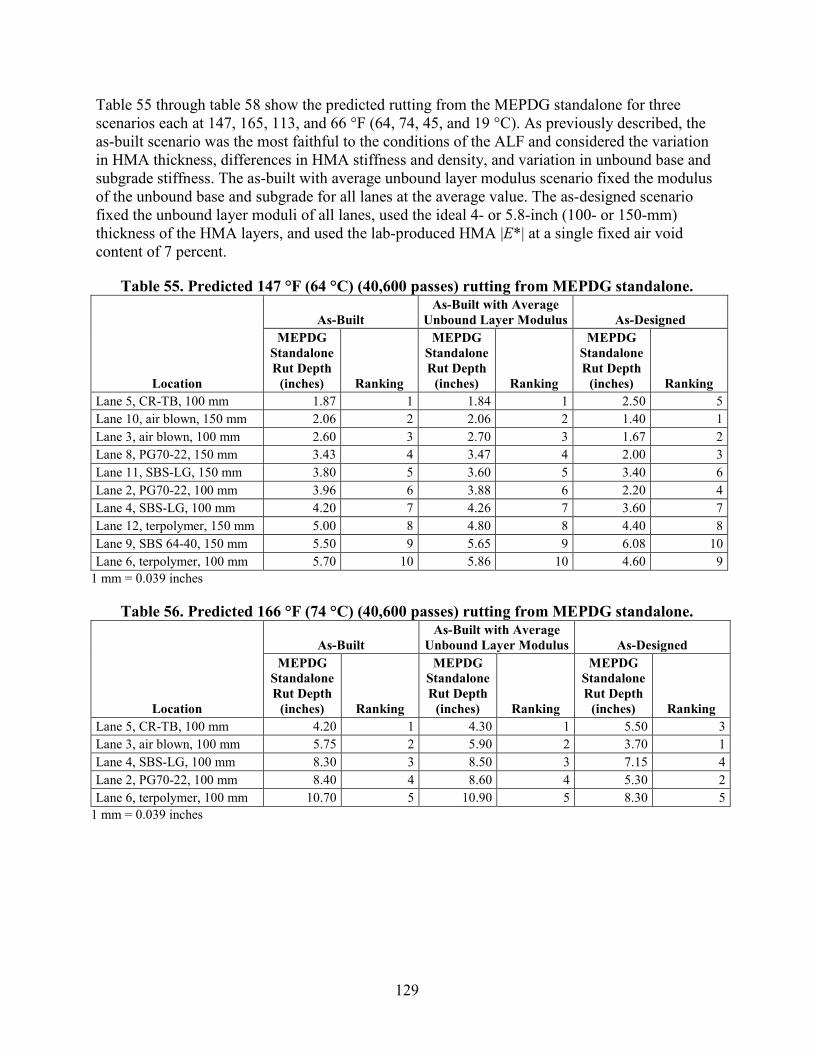
129

Table 55 through table 58 show the predicted rutting from the MEPDG standalone for three scenarios each at 147, 165, 113, and 66 °F (64, 74, 45, and 19 °C). As previously described, the as-built scenario was the most faithful to the conditions of the ALF and considered the variation in HMA thickness, differences in HMA stiffness and density, and variation in unbound base and subgrade stiffness. The as-built with average unbound layer modulus scenario fixed the modulus of the unbound base and subgrade for all lanes at the average value. The as-designed scenario fixed the unbound layer moduli of all lanes, used the ideal 4- or 5.8-inch (100- or 150-mm) thickness of the HMA layers, and used the lab-produced HMA |E*| at a single fixed air void content of 7 percent.

Table 55. Predicted 147 °F (64 °C) (40,600 passes) rutting from MEPDG standalone.

Location

As-Built As-Built with Average

Unbound Layer Modulus As-Designed MEPDG

Standalone Rut Depth

(inches) Ranking

MEPDG Standalone Rut Depth

(inches) Ranking

MEPDG Standalone Rut Depth

(inches) Ranking Lane 5, CR-TB, 100 mm 1.87 1 1.84 1 2.50 5 Lane 10, air blown, 150 mm 2.06 2 2.06 2 1.40 1 Lane 3, air blown, 100 mm 2.60 3 2.70 3 1.67 2 Lane 8, PG70-22, 150 mm 3.43 4 3.47 4 2.00 3 Lane 11, SBS-LG, 150 mm 3.80 5 3.60 5 3.40 6 Lane 2, PG70-22, 100 mm 3.96 6 3.88 6 2.20 4 Lane 4, SBS-LG, 100 mm 4.20 7 4.26 7 3.60 7 Lane 12, terpolymer, 150 mm 5.00 8 4.80 8 4.40 8 Lane 9, SBS 64-40, 150 mm 5.50 9 5.65 9 6.08 10 Lane 6, terpolymer, 100 mm 5.70 10 5.86 10 4.60 9

1 mm = 0.039 inches

Table 56. Predicted 166 °F (74 °C) (40,600 passes) rutting from MEPDG standalone.

Location

As-Built As-Built with Average

Unbound Layer Modulus As-Designed MEPDG

Standalone Rut Depth

(inches) Ranking

MEPDG Standalone Rut Depth

(inches) Ranking

MEPDG Standalone Rut Depth

(inches) Ranking Lane 5, CR-TB, 100 mm 4.20 1 4.30 1 5.50 3 Lane 3, air blown, 100 mm 5.75 2 5.90 2 3.70 1 Lane 4, SBS-LG, 100 mm 8.30 3 8.50 3 7.15 4 Lane 2, PG70-22, 100 mm 8.40 4 8.60 4 5.30 2 Lane 6, terpolymer, 100 mm 10.70 5 10.90 5 8.30 5

1 mm = 0.039 inches

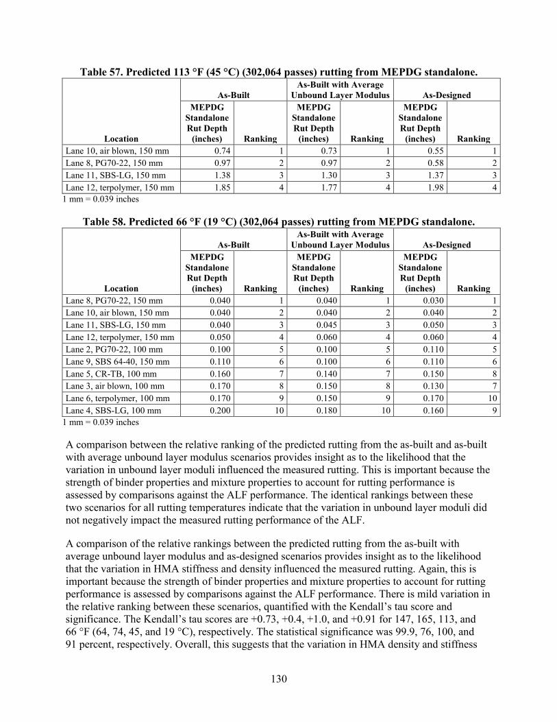
130

Table 57. Predicted 113 °F (45 °C) (302,064 passes) rutting from MEPDG standalone.

Location

As-Built As-Built with Average

Unbound Layer Modulus As-Designed MEPDG

Standalone Rut Depth

(inches) Ranking

MEPDG Standalone Rut Depth

(inches) Ranking

MEPDG Standalone Rut Depth

(inches) Ranking Lane 10, air blown, 150 mm 0.74 1 0.73 1 0.55 1 Lane 8, PG70-22, 150 mm 0.97 2 0.97 2 0.58 2 Lane 11, SBS-LG, 150 mm 1.38 3 1.30 3 1.37 3 Lane 12, terpolymer, 150 mm 1.85 4 1.77 4 1.98 4

1 mm = 0.039 inches

Table 58. Predicted 66 °F (19 °C) (302,064 passes) rutting from MEPDG standalone.

Location

As-Built As-Built with Average

Unbound Layer Modulus As-Designed MEPDG

Standalone Rut Depth

(inches) Ranking

MEPDG Standalone Rut Depth

(inches) Ranking

MEPDG Standalone Rut Depth

(inches) Ranking Lane 8, PG70-22, 150 mm 0.040 1 0.040 1 0.030 1 Lane 10, air blown, 150 mm 0.040 2 0.040 2 0.040 2 Lane 11, SBS-LG, 150 mm 0.040 3 0.045 3 0.050 3 Lane 12, terpolymer, 150 mm 0.050 4 0.060 4 0.060 4 Lane 2, PG70-22, 100 mm 0.100 5 0.100 5 0.110 5 Lane 9, SBS 64-40, 150 mm 0.110 6 0.100 6 0.110 6 Lane 5, CR-TB, 100 mm 0.160 7 0.140 7 0.150 8 Lane 3, air blown, 100 mm 0.170 8 0.150 8 0.130 7 Lane 6, terpolymer, 100 mm 0.170 9 0.150 9 0.170 10 Lane 4, SBS-LG, 100 mm 0.200 10 0.180 10 0.160 9

1 mm = 0.039 inches

A comparison between the relative ranking of the predicted rutting from the as-built and as-built with average unbound layer modulus scenarios provides insight as to the likelihood that the variation in unbound layer moduli influenced the measured rutting. This is important because the strength of binder properties and mixture properties to account for rutting performance is assessed by comparisons against the ALF performance. The identical rankings between these two scenarios for all rutting temperatures indicate that the variation in unbound layer moduli did not negatively impact the measured rutting performance of the ALF.

A comparison of the relative rankings between the predicted rutting from the as-built with average unbound layer modulus and as-designed scenarios provides insight as to the likelihood that the variation in HMA stiffness and density influenced the measured rutting. Again, this is important because the strength of binder properties and mixture properties to account for rutting performance is assessed by comparisons against the ALF performance. There is mild variation in the relative ranking between these scenarios, quantified with the Kendall’s tau score and significance. The Kendall’s tau scores are +0.73, +0.4, +1.0, and +0.91 for 147, 165, 113, and 66 °F (64, 74, 45, and 19 °C), respectively. The statistical significance was 99.9, 76, 100, and 91 percent, respectively. Overall, this suggests that the variation in HMA density and stiffness

131

had a weak effect on the measured performance, except at 165 °F (74 °C). This could in part be because there were fewer data points at 165 °F (74 °C). Nonetheless, it must be recognized that the predicted rutting was impractically large for the three highest temperatures without lateral wheel wander.

Influence of Construction Variability on Fatigue Cracking

Predicted bottom-up fatigue cracking from the MEPDG standalone program is shown in figure 97 through figure 99 for the three different scenarios. Ranked predicted fatigue cracking is shown in table 58. The shape of the predicted cracking curve is smooth and continuously increasing from the beginning at zero passes. This is a marked difference from the measured pattern of cracking where no fatigue cracks are registered until they reach the surface and then increase in an almost linear fashion. Again, this is merely an observation, not a criticism of the nationally calibrated MEPDG. Unlike predicted rutting, the fatigue cracking curves from the different mixtures and lanes can crisscross.

Figure 97. Graph. Percent fatigue cracking predicted from MEPDG standalone program

for the as-built scenario.

Site 3 19oC As-Built HMA Fatigue

-

5

10

15

20

25

30

35

40

45

- 50,000 100,000 150,000 200,000 250,000 300,000 350,000 400,000 450,000

Number of Passes

Perc

ent C

rack

ing

Lane 6, Terpolymer, 100mm Lane 4, SBS-LG, 100mm

Lane 5, CRTB, 100mm

Lane 3, Air Blown, 100mm

Lane 9, SBS 64-40, 150mm

Lane 2, Control, 100mm

Lane 12, Terpolymer, 150mm

Lane 11, SBS-LG, 150mm Lane 10, Air Blown, 150mm Lane 8, Control, 150mm

132

Figure 98. Graph. Percent fatigue cracking predicted from MEPDG standalone program

for the as-built with average unbound layer modulus scenario.

Figure 99. Graph. Percent fatigue cracking predicted from MEPDG standalone program

for the as-designed scenario.

Site 3 19oC As-Built + As-Des. Unbound HMA Fatigue

-

5

10

15

20

25

30

35

40

45

- 50,000 100,000 150,000 200,000 250,000 300,000 350,000 400,000 450,000

Number of Passes

Perc

ent C

rack

ing

Lane 6, Terpolymer, 100mm

Lane 4, SBS-LG, 100mm

Lane 5, CRTB, 100mm

Lane 3, Air Blown, 100mm

Lane 9, SBS 64-40, 150mm

Lane 2, Control, 100mm

Lane 12, Terpolymer, 150mm Lane 11, SBS-LG, 150mm

Lane 10, Air Blown, 150mm

Lane 8, Control, 150mm

Site 3, 19oC As-Designed HMA Fatigue Cracking

-

5.00

10.00

15.00

20.00

25.00

30.00

35.00

- 50,000 100,000 150,000 200,000 250,000 300,000 350,000 400,000 450,000

Number of Passes

Perc

ent C

rack

ing

Lane 6, Terpolymer, 100mm

Lane 4, SBS-LG, 100mm Lane 5, CRTB, 100mm

Lane 3, Air Blown, 100mm

Lane 9, SBS 64-40, 150mm

Lane 2, Control, 100mm

Lane 12, Terpolymer, 150mm Lane 11, SBS-LG, 150mm

Lane 10, Air Blown, 150mm Lane 8, Control, 150mm

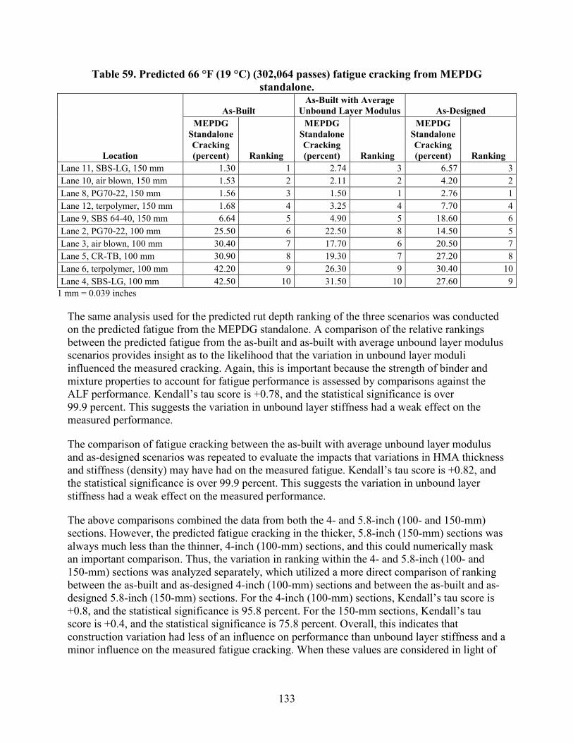
133

Table 59. Predicted 66 °F (19 °C) (302,064 passes) fatigue cracking from MEPDG standalone.

Location

As-Built As-Built with Average

Unbound Layer Modulus As-Designed MEPDG

Standalone Cracking (percent) Ranking

MEPDG Standalone Cracking (percent) Ranking

MEPDG Standalone Cracking (percent) Ranking

Lane 11, SBS-LG, 150 mm 1.30 1 2.74 3 6.57 3 Lane 10, air blown, 150 mm 1.53 2 2.11 2 4.20 2 Lane 8, PG70-22, 150 mm 1.56 3 1.50 1 2.76 1 Lane 12, terpolymer, 150 mm 1.68 4 3.25 4 7.70 4 Lane 9, SBS 64-40, 150 mm 6.64 5 4.90 5 18.60 6 Lane 2, PG70-22, 100 mm 25.50 6 22.50 8 14.50 5 Lane 3, air blown, 100 mm 30.40 7 17.70 6 20.50 7 Lane 5, CR-TB, 100 mm 30.90 8 19.30 7 27.20 8 Lane 6, terpolymer, 100 mm 42.20 9 26.30 9 30.40 10 Lane 4, SBS-LG, 100 mm 42.50 10 31.50 10 27.60 9

1 mm = 0.039 inches

The same analysis used for the predicted rut depth ranking of the three scenarios was conducted on the predicted fatigue from the MEPDG standalone. A comparison of the relative rankings between the predicted fatigue from the as-built and as-built with average unbound layer modulus scenarios provides insight as to the likelihood that the variation in unbound layer moduli influenced the measured cracking. Again, this is important because the strength of binder and mixture properties to account for fatigue performance is assessed by comparisons against the ALF performance. Kendall’s tau score is +0.78, and the statistical significance is over 99.9 percent. This suggests the variation in unbound layer stiffness had a weak effect on the measured performance.

The comparison of fatigue cracking between the as-built with average unbound layer modulus and as-designed scenarios was repeated to evaluate the impacts that variations in HMA thickness and stiffness (density) may have had on the measured fatigue. Kendall’s tau score is +0.82, and the statistical significance is over 99.9 percent. This suggests the variation in unbound layer stiffness had a weak effect on the measured performance.

The above comparisons combined the data from both the 4- and 5.8-inch (100- and 150-mm) sections. However, the predicted fatigue cracking in the thicker, 5.8-inch (150-mm) sections was always much less than the thinner, 4-inch (100-mm) sections, and this could numerically mask an important comparison. Thus, the variation in ranking within the 4- and 5.8-inch (100- and 150-mm) sections was analyzed separately, which utilized a more direct comparison of ranking between the as-built and as-designed 4-inch (100-mm) sections and between the as-built and as-designed 5.8-inch (150-mm) sections. For the 4-inch (100-mm) sections, Kendall’s tau score is +0.8, and the statistical significance is 95.8 percent. For the 150-mm sections, Kendall’s tau score is +0.4, and the statistical significance is 75.8 percent. Overall, this indicates that construction variation had less of an influence on performance than unbound layer stiffness and a minor influence on the measured fatigue cracking. When these values are considered in light of

134

the actual, wider differences in measured fatigue cracking under the ALF, the ranking of the sections may not have changed significantly if constructed at the ideal density and thickness.

Assessment of MEPDG Predictive Capability

As previously stated, it is unfair to expect a high degree of predictive accuracy of the MEPDG for the ALF test sections because the MEPDG uses a national calibration, the national calibration is based almost entirely on HMA mixtures having unmodified asphalt binders, and the heavy wheel loads and intense number of cycles challenge the calibration that took place under more natural traffic. Only the relative order of measured versus predicted distress is compared rather than absolute predictive capability, and the analysis should not be taken as a weakness or negative departure from the intended use of the MEPDG. As the name suggests, the MEPDG is meant to provide design guidance to practitioners. As implementation proceeds, the primary utilization of the MEPDG will be to understand relative changes in performance due to the consequences of changing a particular layer’s material, stiffness, thickness, etc.

Rutting

MEPDG standalone rutting was compared against measured rutting at all temperatures, and all 4- and 5.8-inch (100- and 150-mm) data points were combined. The rut depths at a fixed number of load cycles under the ALF and calculated by the MEPDG standalone were directly compared against one another. The number of cycles at which the measured and predicted rutting were compared depended on the temperature of the test and thickness of the HMA layer. At 66 °F (19 °C), where lateral wheel wander was utilized for fatigue cracking, the rutting was compared at 100,000 cycles for the 4-inch (100-mm) lanes and at 300,000 cycles for the 5.8-inch (150-mm) lanes. At 113, 147, and 165 °F (45, 64, and 74 °C), the rutting was compared at 200,000, 25,000, and 10,000 cycles, respectively. The average measured rutting for these comparisons was 0.4 inches (9.8 mm). The minimum and maximum measured rutting were 0.1 and 0.7 inches (3.3 and 17.3 mm).

The as-built with average unbound layers scenario was not considered. Two extreme simulation scenarios were considered, as-built and as-designed, and are shown in figure 100 and figure 101, respectively. It is clear that the rutting from higher temperatures without lateral wheel wander was over-predicted, while the rutting from the 66 °F (19 °C) intermediate temperature with lateral wheel wander was under-predicted. As noted previously, large impractical rutting does not necessarily detract from the MEPDG because of the calibration and ALF conditions. Regardless of which simulation scenario is considered, the MEPDG does account for different amounts of rutting at different temperatures and cycles. There is a positive proportional relationship between measured and predicted rutting. Kendall’s tau parameters from as-built and as-designed inputs were +0.50 and +0.46, respectively. The significance of the regression from as-built and as-designed inputs were 99.99 percent (a p-value of 0.001 percent) and 99.9 percent (a p-value of 0.010 percent), respectively. R from as-built and as-designed inputs were +0.71 and +0.66, respectively. R2 from as-built and as-designed scenarios were 0.51 and 0.43, respectively.

135

1 mm = 0.039 inches

Figure 100. Graph. Measured ALF rutting versus MEPDG standalone-predicted rutting for the as-built scenario.

1 mm = 0.039 inches

Figure 101. Graph. Measured ALF rutting versus MEPDG standalone-predicted rutting for the as-designed scenario.

0.00

2.00

4.00

6.00

8.00

10.00

12.00

14.00

16.00

18.00

20.00

0 20 40 60 80 100 120 140 160MEPDG Stand Alone Predicted Rutting (mm)

ALF

Mea

sure

d R

uttin

g (m

m)

64C 100mm & 150mm74C 100mm & 150mm45C 150mm19C 100mm19C 150mmLine of EqualityAs-Built Simulation

0.00

2.00

4.00

6.00

8.00

10.00

12.00

14.00

16.00

18.00

20.00

0 20 40 60 80 100 120 140 160MEPDG Stand Alone Predicted Rutting (mm)

ALF

Mea

sure

d R

uttin

g (m

m)

64C 100mm & 150mm74C 100mm & 150mm45C 150mm19C 100mm19C 150mmLine of EqualityAs-Designed Simulation

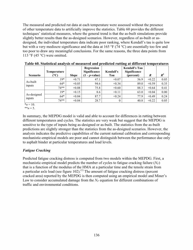
136

The measured and predicted rut data at each temperature were assessed without the presence of other temperature data to artificially improve the statistics. Table 60 provides the different techniques’ statistical measures, where the general trend is that the as-built simulations provide slightly better results than the as-designed scenarios. However, regardless of as-built or as-designed, the individual temperature data indicate poor ranking, where Kendall’s tau is quite low but with a very mediocre significance and the data at 165 °F (74 °C) are essentially too few and too poor to draw any meaningful conclusions. For the same reasons, the three data points from 113 °F (45 °C) were omitted.

Table 60. Statistical analysis of measured and predicted rutting at different temperatures

Scenario Temperature

(°C) Slope

Regression Significance (1 – p-value)

Kendall’s Tau

Kendall’s Tau Significance

(percent) R R2

As-built inputs

19* +0.71 47.1 +0.07 56.9 +0.22 0.05 64* +0.05 94.6 +0.34 89.0 +0.59 0.35

74** +0.08 75.8 +0.60 88.3 +0.64 0.41

As-designed inputs

19* +0.15 8.6 +0.11 63.0 +0.04 0.00 64* +0.04 87.7 +0.24 77.9 +0.49 0.24

74** +0.04 28.7 0 40.8 +0.22 0.05 *n = 10. **n = 5.

In summary, the MEPDG model is valid and able to account for differences in rutting between different temperatures and cycles. The statistics are very weak but suggest that the MEPDG is sensitive to the type of inputs being as-designed or as-built. The statistics from the as-built predictions are slightly stronger than the statistics from the as-designed scenarios. However, the analysis indicates the predictive capabilities of the current national calibration and corresponding mechanistic-empirical models are poor and cannot distinguish between the performance due only to asphalt binder at particular temperatures and load levels.

Fatigue Cracking

Predicted fatigue cracking distress is computed from two models within the MEPDG. First, a mechanistic-empirical model predicts the number of cycles to fatigue cracking failure (NF) that is a function of the modulus of the HMA at a particular time and the tensile strain from a particular axle load (see figure 102).(1) The amount of fatigue cracking distress (percent cracked area) reported by the MEPDG is then computed using an empirical model and Miner’s Law to consider accumulated damage from the NF equation for different combinations of traffic and environmental conditions.

137

( ) 43

1100432.0 1

kk

TF EkCN

= ε

Figure 102. Equation. Cycles to fatigue cracking failure.

Where:

( )

+−

=

−

+=

=

− AC

M

h

ab

b

e

k

VVVM

C

49.302.11

1

1003602.0000398.0

1

69.084.4

10

Tε = HMA tensile strain (mm/mm or inch/inch). E = HMA modulus (psi). Va = Air void content (percent). Vb = Effective volume of binder (percent). hAC = Thickness of HMA (inches).

Two methods were used to assess the predictive capability of the MEPDG. Standard output of percent cracked area from the MEPDG standalone was directly compared to the cracked area from ALF. The number of ALF cycles to achieve 25 percent cracked area, which is equivalent to 7.75 percent MEPDG cracked area, was compared to the predicted number of cycles to 7.75 percent cracked area. Also, the internal mechanistic-empirical NF model was evaluated by comparing the number of ALF cycles to initiate surface cracks and calculated number of cycles to failure computed from the known strains in table 54 and known |E*| dynamic moduli in table 52.

Measured fatigue cracking data in chapter 3 clearly show that many more cycles were required to induce fatigue cracking in the thicker 5.8-inch (150-mm) lanes than in the thinner 4-inch (100-mm) lanes and that additional analyses using extrapolation and interpolation were needed to develop a complete set of ranked performance to common criteria. The comparison between measured and predicted number of cycles to 7.75 percent cracked area is shown in arithmetic scale in figure 103 and in log-log scale in figure 104 to highlight the fatigue cracking data points from the 4-inch (100-mm) sections. Unlike predicted rutting, the measured and fatigue cracking data points are scattered above and below the line of equality for both the 4- and 5.8-inch (100- and 150-mm) sections. The predicted fatigue cracking is still qualitatively inaccurate but not as impractical as the predicted rutting. Also unlike rutting, the trends become negative instead of proportionally positive when a smaller data subset is evaluated. Smaller sets of temperature data were evaluated in rutting, and smaller sets of thickness were evaluated in fatigue.

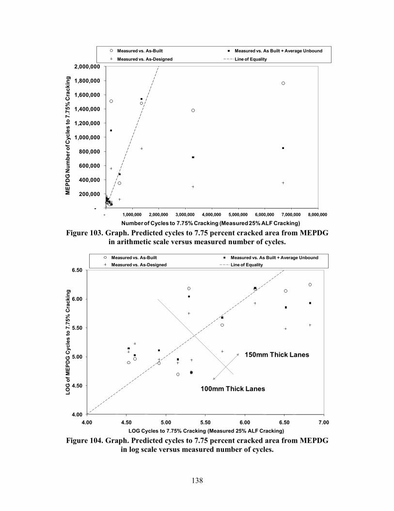
138

Figure 103. Graph. Predicted cycles to 7.75 percent cracked area from MEPDG

in arithmetic scale versus measured number of cycles.

Figure 104. Graph. Predicted cycles to 7.75 percent cracked area from MEPDG

in log scale versus measured number of cycles.

-

200,000

400,000

600,000

800,000

1,000,000

1,200,000

1,400,000

1,600,000

1,800,000

2,000,000

- 1,000,000 2,000,000 3,000,000 4,000,000 5,000,000 6,000,000 7,000,000 8,000,000

MEP

DG

Num

ber o

f Cyc

les

to 7

.75%

Cra

ckin

g

Number of Cycles to 7.75% Cracking (Measured 25% ALF Cracking)

Measured vs. As-Built Measured vs. As Built + Average Unbound

Measured vs. As-Designed Line of Equality

4.00

4.50

5.00

5.50

6.00

6.50

4.00 4.50 5.00 5.50 6.00 6.50 7.00

LOG

of M

EPD

G C

ycle

s to

7.7

5% C

rack

ing

LOG Cycles to 7.75% Cracking (Measured 25% ALF Cracking)

Measured vs. As-Built Measured vs. As Built + Average UnboundMeasured vs. As-Designed Line of Equality

150mm Thick Lanes

100mm Thick Lanes

139

Figure 105 shows the measured number of cycles to achieve surface cracking plotted against the mechanistic-empirical number of cycles to failure computed from figure 102. Although unexpected, the data are distributed on either side of the line of equality. The overall relationship is proportionally positive. The data points from the 4- and 5.8-inch (100- and 150-mm)-thick pavements are not identified in the figure, but data from the 4-inch (100-mm) lanes are in the lower left side, similar to figure 104.

Figure 105. Graph. Predicted cycles to failure from MEPDG equation in arithmetic scale

versus measured number of cycles to surface crack initiation.

Table 61 contains the statistical measures for the various comparisons of ALF performance with MEPDG cracking output and the internal mechanistic-empirical model for number of cycles to failure. The trends are essentially very weak but go in the correct direction when data from both 4- and 5.8-inch (100- and 150–mm) lanes are considered together. The regression slope, Kendall’s tau, and correlation coefficient are all positive, but the statistical significance is smaller than conventionally desired, such as above 90 percent. The trends appear to get weaker as the simulation scenario diverges from as-built to as-designed. However, when only the 4-inch (100-mm) lanes are considered (where the dataset is more complete than the 5.8-inch (150-mm) lanes), the comparisons are worse in both cases of cracking output and number of cycles to failure. Although the strength of the relationships between measured and predicted is stronger, the direction of the relationship is now inverse and not reasonable.

-

100,000

200,000

300,000

400,000

500,000

600,000

700,000

- 100,000 200,000 300,000 400,000 500,000 600,000 700,000 800,000

NF

MEP

DG

Inte

rnal

Mod

el

Measured Cycles to Surface Crack Initiation

As-Built HMA Modulus As-Designed HMA Modulus Line of Equality

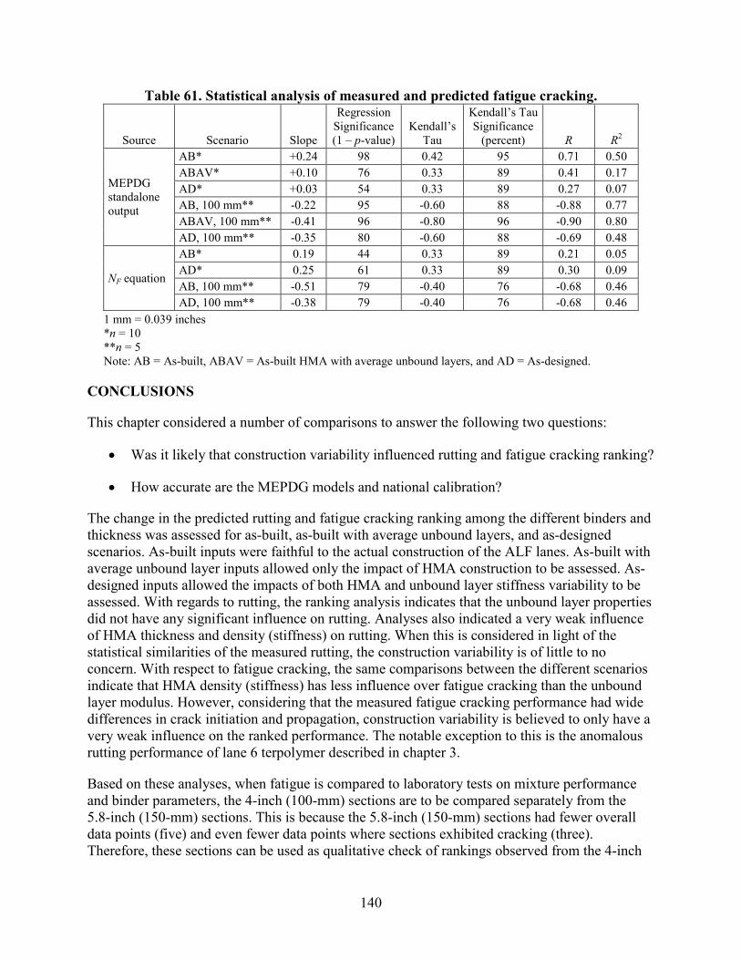
140

Table 61. Statistical analysis of measured and predicted fatigue cracking.

Source Scenario Slope

Regression Significance (1 – p-value)

Kendall’s Tau

Kendall’s Tau Significance

(percent) R R2

MEPDG standalone output

AB* +0.24 98 0.42 95 0.71 0.50 ABAV* +0.10 76 0.33 89 0.41 0.17 AD* +0.03 54 0.33 89 0.27 0.07 AB, 100 mm** -0.22 95 -0.60 88 -0.88 0.77 ABAV, 100 mm** -0.41 96 -0.80 96 -0.90 0.80 AD, 100 mm** -0.35 80 -0.60 88 -0.69 0.48

NF equation

AB* 0.19 44 0.33 89 0.21 0.05 AD* 0.25 61 0.33 89 0.30 0.09 AB, 100 mm** -0.51 79 -0.40 76 -0.68 0.46 AD, 100 mm** -0.38 79 -0.40 76 -0.68 0.46

1 mm = 0.039 inches

*n = 10 **n = 5 Note: AB = As-built, ABAV = As-built HMA with average unbound layers, and AD = As-designed.

CONCLUSIONS

This chapter considered a number of comparisons to answer the following two questions:

• Was it likely that construction variability influenced rutting and fatigue cracking ranking?

• How accurate are the MEPDG models and national calibration?

The change in the predicted rutting and fatigue cracking ranking among the different binders and thickness was assessed for as-built, as-built with average unbound layers, and as-designed scenarios. As-built inputs were faithful to the actual construction of the ALF lanes. As-built with average unbound layer inputs allowed only the impact of HMA construction to be assessed. As-designed inputs allowed the impacts of both HMA and unbound layer stiffness variability to be assessed. With regards to rutting, the ranking analysis indicates that the unbound layer properties did not have any significant influence on rutting. Analyses also indicated a very weak influence of HMA thickness and density (stiffness) on rutting. When this is considered in light of the statistical similarities of the measured rutting, the construction variability is of little to no concern. With respect to fatigue cracking, the same comparisons between the different scenarios indicate that HMA density (stiffness) has less influence over fatigue cracking than the unbound layer modulus. However, considering that the measured fatigue cracking performance had wide differences in crack initiation and propagation, construction variability is believed to only have a very weak influence on the ranked performance. The notable exception to this is the anomalous rutting performance of lane 6 terpolymer described in chapter 3.

Based on these analyses, when fatigue is compared to laboratory tests on mixture performance and binder parameters, the 4-inch (100-mm) sections are to be compared separately from the 5.8-inch (150-mm) sections. This is because the 5.8-inch (150-mm) sections had fewer overall data points (five) and even fewer data points where sections exhibited cracking (three). Therefore, these sections can be used as qualitative check of rankings observed from the 4-inch

141

(100-mm) cracking performance. When rutting is evaluated, all 4- and 5.8-inch (100- and 150-mm) data points can be considered together since HMA thickness had less influence on rutting than cracking. However, the same division of data between the 4- and 5.8-inch (100 and 150-mm) ALF performance will be used to assess the laboratory mixture performance tests and binder parameters.

To summarize the evaluation of MEPDG predictive accuracy, the MEPDG seems to be able to tell differences between ALF performance when dissimilar conditions are combined together, such as different temperatures for rutting or different thickness for fatigue cracking. However, the MEPDG does not appear to differentiate between mixtures having only binder as the primary variable at a particular temperature or thickness. Some of this inaccuracy was expected because the ALF conditions were fairly extreme and polymer modified asphalts had very little representation in the national calibration. Finally, although both fatigue and rutting predictions were poor, the MEPDG seems to predict more practical fatigue cracking performance for the ALF conditions than the very impractical predicted rut depth.

143

CHAPTER 5. CANDIDATE BINDER PARAMETERS

INTRODUCTION

As identified in chapter 1, the primary motivation for this research was to identify candidate binder parameters to replace the current Superpave® PG specifications, with special emphasis on fatigue cracking. This chapter describes the development background of various parameters that were identified and gives examples and the quantitative ranking of the ALF binders included in the study.

FATIGUE CRACKING

Superpave® Intermediate Temperature

ALF binder test results from the standard specification test (AASHTO T 315) using DSR to control fatigue cracking at the intermediate temperature range is provided in table 62.(5) Both the specification temperature and the loss modulus at the fixed ALF loading temperature of 66 °F (19 °C) are provided. The unmodified asphalt is the stiffest, and SBS 64-40 modified binder is the softest, with the SBS-LG, CR-TB, and terpolymer modified binders in between.

Table 62. ALF binder standard Superpave® intermediate specification parameters.

Binder

|G*|sin Value at 19 °C, 10 radians/s, 0.4 Percent Strain,

PAV (Pa)

Temperature at |G*|sin = 5 MPa, 10 radians/s, 0.4 Percent Strain,

PAV (°C) PG70-22 12,100,000 26.0 Air blown 6,810,000 22.6 SBS-LG 4,060,000 18.1 CR-TB 4,210,000 17.9 Terpolymer 2,610,000 14.3 CR-AZ — 11.9 SBS 64-40 1,761,800 8.6

1 Pa = 0.000145 psi °F = 1.8(°C) + 32 — Indicates data were not measured.

Superpave® Low-Temperature DT and BBR

Low-temperature failure stress and strain (brittle fracture) from the ALF binders measured in the standard specification test (AASHTO T 314) using the DT test are provided in table 63 along with the BBR creep m-values (AASHTO T 313).(4,3) Failure stress has much less of a trend with temperature than failure strain, and thus failure strains are shown graphically in figure 106, where two of the binders’ failure strains were extrapolated to a common temperature of -11 °F (-24 °C). The rankings of the binders’ failure strains from smallest to largest are PG70-22, air blown, terpolymer, CR-TB, SBS-LG, and SBS 64-40. The creep m-values show the PG70-22, air-blown, SBS-LG, and CR-TB binders have very similar response, while the terpolymer and SBS 64-40 binders have a notably larger, more compliant response (see figure 107).

δ δ

144

Table 63. Low-temperature failure stress, failure strain, and creep m-value.

Binder

DT + BBR Critical

Temp. (°C)

Continuous Low Temp. Grade (°C)

DT and BBR Test Results

Category -6 °C -12 °C -18 °C -24 °C -30 °C -36 °C

PG70-22 -22.4 -23 Failure strain (%) 7.00 1.61 0.60 0.30* — — Failure stress (MPa) 6.35 5.00 4.38 — — — m-value — 0.326 0.302 — — —

Air blown -27.1 -28 Failure strain (%) — 4.12 1.29 0.55 — — Failure stress (MPa) — 4.43 4.89 4.76 — — m-value — 0.330 0.307 0.244 — —

SBS-LG -33.7 -28 Failure strain (%) — — — 1.75 — — Failure stress (MPa) — — — 6.99 — — m-value — — 0.311 0.267 — —

CR-TB -32.9 -28 Failure strain (%) — — 3.91 1.36 — — Failure stress (MPa) — — 4.88 5.74 — — m-value — 0.328 0.315 0.259 — —

Terpolymer -31.1 -31 Failure strain (%) — — 6.63 1.03 — — Failure stress (MPa) — — 5.42 5.88 — — m-value — — 0.370 0.306 — —

SBS 64-40 -36.0 -38 Failure strain (%) — — — 3.00* 1.44 0.75 Failure stress (MPa) — — — — 6.56 6.17 m-value — — 0.399 0.353 0.301 —

°F = 1.8(°C) + 32 1 MPa = 145 psi — Indicates data were not measured. *Semilog extrapolation.

°F = 1.8(°C) + 32

Figure 106. Graph. Failure strain of ALF binders in the low-temperature DT test versus temperature.

0.00

1.00

2.00

3.00

4.00

5.00

6.00

7.00

-42 -36 -30 -24 -18 -12 -6 0

Failu

re St

rain

(%)

Temperature (oC)

Control

Air Blown

SBS-LG

CR-TB

Terpolymer

SBS 64-40

145

°F = 1.8(°C) + 32 Figure 107. Graph. BBR creep m-value of ALF binders versus temperature.

Time Sweep and Stress Sweep

Multiple cycle oscillatory fatigue tests are a classical technique. Such tests impose repeated stresses and strains below the material’s single-cycle strength limit, and the net effect is that damage accumulates, causing the modulus to decrease and the material to ultimately fail. This characterization technique in the DSR was identified in NCHRP 9-10 research for further exploration and implementation as an asphalt binder fatigue parameter.(20)

Martono and Bahia conducted stress sweep and time sweep fatigue testing on the ALF binders in the DSR.(65) Time sweeps are cyclic tests where the imposed oscillatory strain amplitude is fixed throughout the test and fatigue damage is exhibited as the resultant peak-to-peak stresses decrease and, thus, the modulus decreases. A drawback to the time sweep is that it can require many cycles and a significant amount of time before fatigue failure can be reached, which is not ideal for routine specification testing. As the name suggests, a stress sweep consists of multiple cycles of imposed stress magnitude causing the resultant cyclic strain to increase and the modulus to decrease. A special variation of stress sweep fatigue testing was developed by Martono and Bahia as a faster alternative to the time sweep.(65) Instead of fixing the stress amplitude during the test, the stress was exponentially increased to bring failure sooner. A schematic of the two tests is shown in figure 108.

0.2

0.25

0.3

0.35

0.4

0.45

-35 -30 -25 -20 -15 -10

BBR

Cree

p m

-val

ue

Temperature, oC

Control

Air Blown

SBS LG

CR TB

Terpolymer

SBS 64-40

146

Figure 108. Graph. Typical observations during stress sweep and time sweep tests.

Martono and Bahia conducted time sweeps at three strain levels at 66 °F (19 °C) and 10 Hz.(65) The results are summarized in table 64. The binder was RTFO-aged only and was not PAV-aged because the ALF sections were trafficked at a relatively early age. Strain levels between 3 and 9 percent are relatively large and not within the linear viscoelastic range that was estimated to represent the magnitude of strain likely to be encountered at the micromechanical level. The point of failure was defined as when the modulus decreased to 50 percent of the initial (undamaged) modulus. The data indicated some strain sensitivity of fatigue ranking. The ranking of the unmodified binders does not change: air blown performs better than the PG70-22 binder. The CR-TB binder exhibits better performance than terpolymer at the 3 percent strain level, but terpolymer is better at larger strain levels. Also, SBS-LG exhibits superior performance above all binders at all strain levels.

Table 64. Summary of time sweeps from Martono and Bahia.(65)

Binder Percent Strain

Beginning of Test Conditions at Failure Number of Cycles to

Failure, NF (x 1,000)

|G*| (MPa)

Phase Angle

(degrees) |G*|

(MPa)

Phase Angle

(degrees)

PG70-22 3 23.11 45.46 12.73 46.97 49.63 5 18.16 50.28 9.35 51.51 11.77 7 15.54 53.67 7.65 54.68 4.64

Air blown 3 12.71 44.99 6.48 46.75 108.97 5 10.57 49.06 5.46 51.1 26.02 7 9.36 51.94 4.87 54.18 10.12

SBS LG 5 6.05 49.41 3.02 57.05 1167.1 7 4.99 52.5 2.5 58.58 236.48 9 4.32 54.95 2.16 59.76 71.16

CR-TB 3 5.35 54.21 2.85 55.45 845.43 5 4.37 57 2.24 58.03 51.73 7 3.66 59.1 2.11 60.13 12.63

Terpolymer 3 6.25 50.5 3.29 53.62 532.63 5 5.82 52.74 3.47 55.74 158.67 7 5.17 55.46 3.16 57.79 45.68

1 MPa = 145 psi

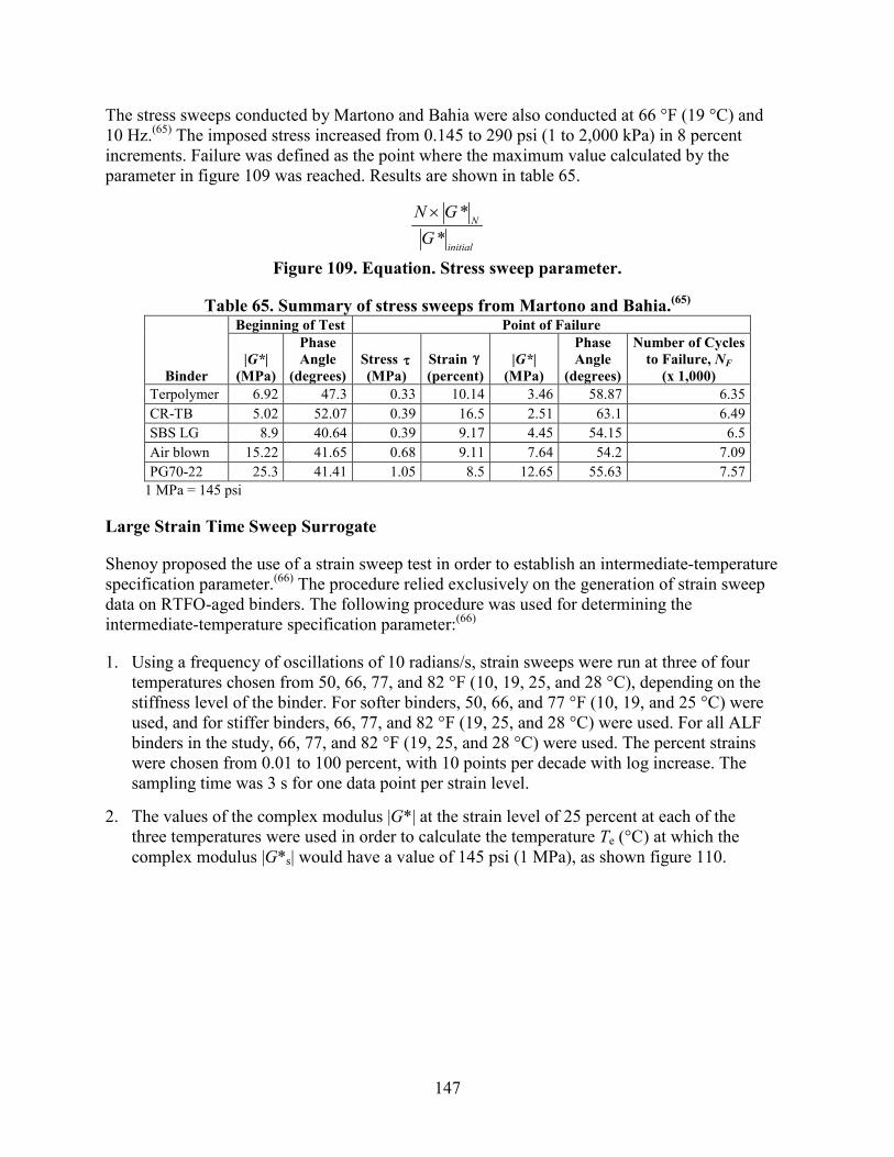
147

The stress sweeps conducted by Martono and Bahia were also conducted at 66 °F (19 °C) and 10 Hz.(65) The imposed stress increased from 0.145 to 290 psi (1 to 2,000 kPa) in 8 percent increments. Failure was defined as the point where the maximum value calculated by the parameter in figure 109 was reached. Results are shown in table 65.

initial

N

GGN

**×

Figure 109. Equation. Stress sweep parameter.

Table 65. Summary of stress sweeps from Martono and Bahia.(65)

Binder

Beginning of Test Point of Failure

|G*| (MPa)

Phase Angle

(degrees) Stress (MPa)

Strain (percent)

|G*| (MPa)

Phase Angle

(degrees)

Number of Cycles to Failure, NF

(x 1,000) Terpolymer 6.92 47.3 0.33 10.14 3.46 58.87 6.35 CR-TB 5.02 52.07 0.39 16.5 2.51 63.1 6.49 SBS LG 8.9 40.64 0.39 9.17 4.45 54.15 6.5 Air blown 15.22 41.65 0.68 9.11 7.64 54.2 7.09 PG70-22 25.3 41.41 1.05 8.5 12.65 55.63 7.57

1 MPa = 145 psi

Large Strain Time Sweep Surrogate

Shenoy proposed the use of a strain sweep test in order to establish an intermediate-temperature specification parameter.(66) The procedure relied exclusively on the generation of strain sweep data on RTFO-aged binders. The following procedure was used for determining the intermediate-temperature specification parameter:(66)

1. Using a frequency of oscillations of 10 radians/s, strain sweeps were run at three of four temperatures chosen from 50, 66, 77, and 82 °F (10, 19, 25, and 28 °C), depending on the stiffness level of the binder. For softer binders, 50, 66, and 77 °F (10, 19, and 25 °C) were used, and for stiffer binders, 66, 77, and 82 °F (19, 25, and 28 °C) were used. For all ALF binders in the study, 66, 77, and 82 °F (19, 25, and 28 °C) were used. The percent strains were chosen from 0.01 to 100 percent, with 10 points per decade with log increase. The sampling time was 3 s for one data point per strain level.

2. The values of the complex modulus |G*| at the strain level of 25 percent at each of the three temperatures were used in order to calculate the temperature Te (°C) at which the complex modulus |G*s| would have a value of 145 psi (1 MPa), as shown figure 110.

τ γ

148

1 Pa = 0.000145 psi °F = 1.8(°C) + 32

Figure 110. Graph. Complex shear modulus and temperature during 25 percent controlled strain test.

3. The values of the loss modulus G''s = |G*|sin s at the strain level of 25 percent at each of the three temperatures were used in order to calculate the value of the loss modulus G''s at the temperature Te (°C), as shown in figure 111.

1 Pa = 0.000145 psi °F = 1.8(°C) + 32

Figure 111. Graph. Loss modulus and temperature during 25 percent controlled strain test.

4. The intermediate-temperature specification TIS was then calculated as Te (G''s /|G*s|) or Te sin s and was used for ranking the binders in terms of their expected fatigue performance.

Test results on the ALF binders are provided in table 66.

δ

δ

149

Table 66. Shenoy’s large strain intermediate stiffness and temperature.

Binder

|G*|sin 19 °C, 10 radians/s,

25 Percent Strain, RTFO (Pa)

TEsin s TE at |G*s| = 1 MPa, 10 radians/s,

25 Percent Strain, RTFO (°C) PG70-22 3,940,000 28.1 Air blown 2,390,000 24.8 CR-TB 1,280,000 19.1 SBS-LG 1,360,000 19.2 Terpolymer 910,000 16.8 SBS 64-40 489,000 11.3

1 Pa = 0.000145 psi °F = 1.8(°C) + 32

Critical Tip Opening Displacement and Essential Work of Fracture

Queen’s University researchers proposed evaluation of the energy needed for fracturing ductile materials to get a measure of the fatigue and crack resistance behavior of asphalt binders.(67) The essential work of fracture (EWF) approach has a history of application in the failure characterization of ductile materials such as plastics, certain metals, and composite materials.(68–70) Prior to the development of the EWF method, the fracture resistance of viscoplastic materials was largely evaluated by using laborious techniques requiring explicit measurements of a crack advancing through material. There had been many attempts to evaluate the work required to create new surfaces in intact material (i.e., cracking). The work necessary to pull apart a prenotched elastoplastic specimen is assumed to be divided in two parts: essential work performed in the local region of the advancing crack creating two surfaces and non-essential work away from the local region of cracking/tearing associated with ductility, plasticity, and yielding.(69)

The experimental determination of the essential and non-essential work of fracture involves the following steps. First, total work of fracture is determined in simple DT tests of similar specimens with different ligament lengths. Double edged notched tension (DENT) samples were used in the characterization of ALF following a protocol developed in Ontario Ministry of Transportation Test Method LS-299.(71) Figure 112 is a schematic of the sample in the DENT test defining ligament length, and figure 113 shows the test samples in a computer-controlled force-ductility instrument. Figure 114 provides an example of raw force versus displacement data after a DENT test using three ligament lengths and two replicates for each ligament. The ALF binders were PAV-aged instead of only RTFO-aged. The test temperature was 77 °F (25 °C), and the extension rate was 4 inches/min (100 mm/min). Ligament lengths were 0.2, 0.4, and 0.58 inches (5, 10, and 15 mm). The areas underneath the force versus displacement curves in figure 114 represent the total work of fracture. These values divided by the sectional area of each corresponding ligament (0.2, 0.4, and 0.58 inches (5, 10, and 15 mm) multiplied by 0.25 inches (6.5 mm) representing the sample thickness) represent the total specific work of fracture. Second, the values of the specific fracture energies are plotted on a graph versus the ligament lengths. A straight line results when total specific work of fracture, Wf, is plotted against ligament length, as shown in figure 115.

δ δ

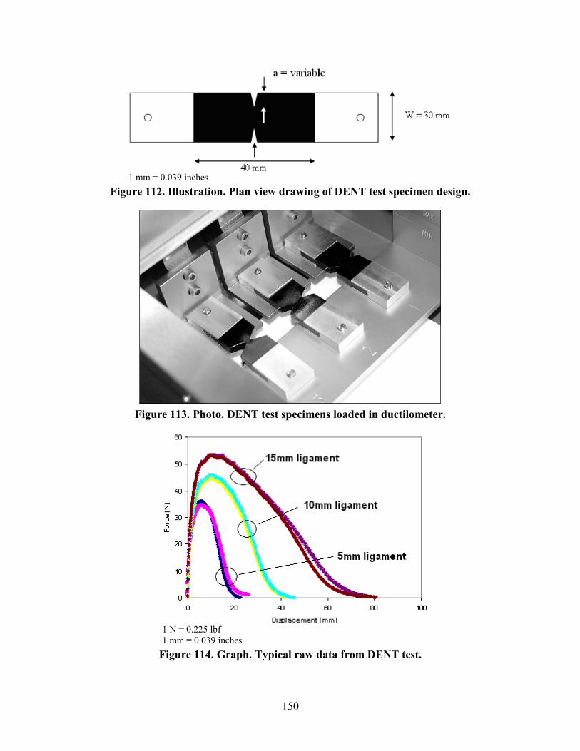
150

1 mm = 0.039 inches

Figure 112. Illustration. Plan view drawing of DENT test specimen design.

Figure 113. Photo. DENT test specimens loaded in ductilometer.

1 N = 0.225 lbf 1 mm = 0.039 inches

Figure 114. Graph. Typical raw data from DENT test.

151

1 J/m2 = 0.0685 lb-ft/ft2 1 m = 3.28 ft Figure 115. Graph. Total work of fracture versus ligament length.

Some background on the mathematics is provided for clarity. The EWF, We, is proportional to the fracture area (i.e., ligament length, l, multiplied by thickness, B), while the non-essential or plastic work, Wp, is proportional to the volume of the plastic zone. This is fracture area (l × B) multiplied by ligament length, multiplied with factor . The factor depends on the shape of the plastic zone. Because the ligament length has major importance in determining the extent of plastic deformation, it is distinctly incorporated as l × and multiplied with the surface area to express the volume dependence of the plastic work of fracture, Wp. The rather simple mathematical expression for the total work of fracture, Wf, is as shown in figure 116.

Figure 116. Equation. Total work of fracture.

Where:

Wf = Total work of fracture. We = EWF. Wp = Total plastic work of fracture. l = Ligament length. B = Thickness. we = Specific essential work of fracture . wp = Specific work of fracture.

The parameter is determined considering the degree to which the sample geometry follows plane-strain or plane-stress conditions. In this scenario, is calculated as shown in figure 117.

Figure 117. Equation. DENT beta parameter.

y = 524263x + 6492.6R2 = 0.9675

0

2000

4000

6000

8000

10000

12000

14000

16000

0 0.002 0.004 0.006 0.008 0.01 0.012 0.014 0.016

L(m)

Wt(j

/m2)

β β

β

Wf = We + Wp = lBwe + βl2Bwp

β β

152

Where:

h = Height of an assumed elliptic shape of the plastic zone. L = Ligament length.

Using a linear fitting procedure similar to the one employed for the EWF analysis, the calculated critical tip opening displacement (CTOD), , is the ultimate elongation for a zero ligament length, which represents the strain tolerance in the vicinity of a crack. In this study, the tensile yield stress was approximated with the net section stress (peak load divided by the sectional area) for the smallest ligament length (0.2 inches (5 mm)). This allowed an approximate CTOD to be calculated from the ratio between the essential work and the net section stress, as shown in figure 118.

Figure 118. Equation. Approximate CTOD.

EWF and CTOD test results on the ALF binders are provided in table 67 along with the yield stress at the smallest ligament length (0.2 inches (5 mm)). The polymer modified binders have the largest CTOD, and the unmodified binders have the lowest. There is a general trend of rank in EWF, but this is not the case for the yield stress. The EWF and CTOD testing methodologies were carried out on mixtures under different conditions, as discussed in the next chapter. Furthermore, the results from an Ontario Ministry of Transportation field test will be discussed in light of the statistical comparison methodologies in chapter 7.

Table 67. Ranked test results by CTOD with EWF and yield stress.

Binder EWF

(kJ/m2) Yield Stress

(kPa) Calculated

CTOD (mm) SBS 64-40 4.4 102 43.1 CR-AZ 10.6 249 42.6 SBS-LG 1.02 43 24.0 Terpolymer 0.85 54 15.7 CR-TB 0.60 71 8.5 PG70-22 0.97 129 7.5 Air blown 0.70 103 6.8

1 kJ = 23,730 lb-ft2/s2 1 kPa = 0.145 psi 1 mm = 0.039 inches

Yield Energy

Johnson et al. suggested the use of the yield energy to identify the relative performance of asphalt binders.(72) The method involves the evaluation of the amount of energy to cause yielding in the asphalt binder. PAV-aged binder is tested in the DSR using the 0.3-inch (8-mm) parallel plate with a 0.08-inch (2-mm) gap. The sample is subjected to monotonic shear using a constant shear rate until peak strength is achieved and the sample yields. At the temperature of interest, a constant shear rate of 1 percent strain per second is used, and the test is continued until the material achieves 3,600 percent strain in 60 min. The shear stress and the shear strain percent are recorded at a sampling rate of one data point every 2 s. A typical plot of the shear stress versus shear strain is shown in figure 119. The ranked results are shown in table 68.

δ

δ = We/σ

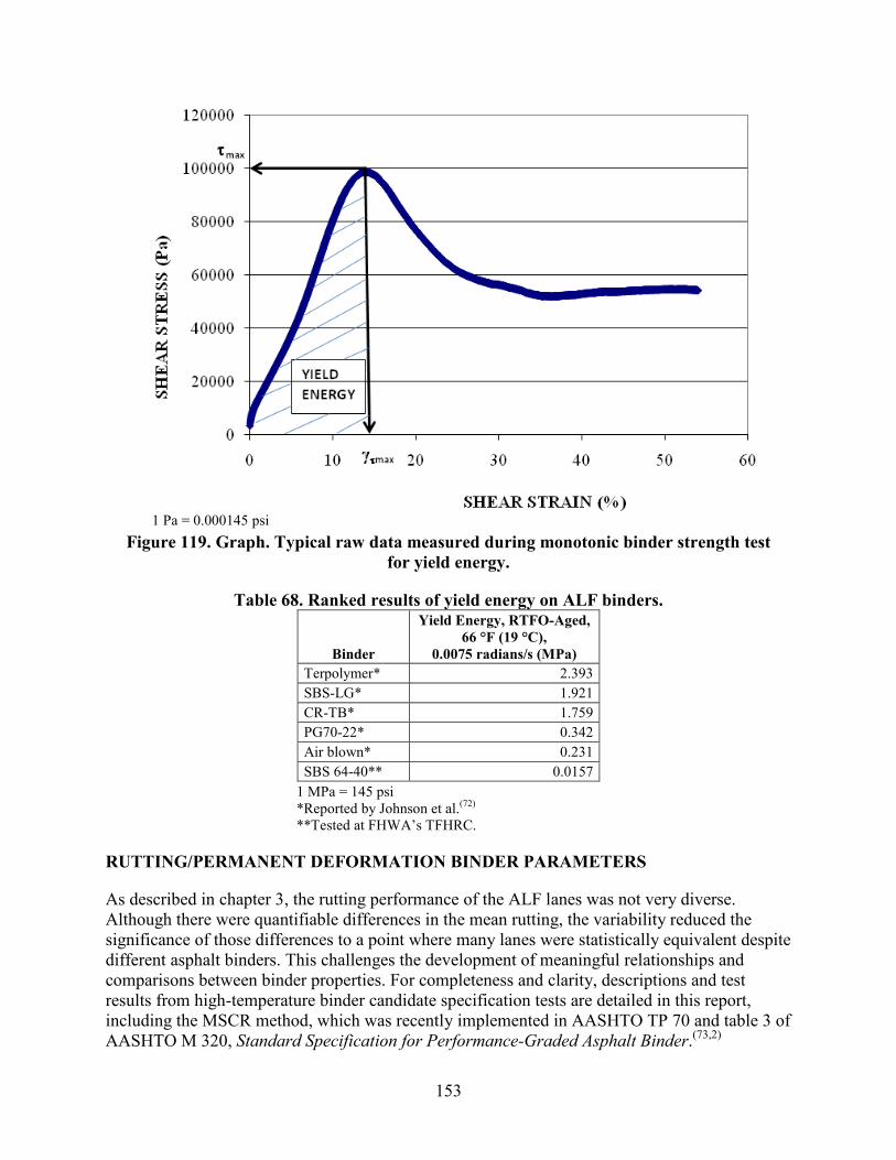
153

1 Pa = 0.000145 psi

Figure 119. Graph. Typical raw data measured during monotonic binder strength test for yield energy.

Table 68. Ranked results of yield energy on ALF binders.

Binder

Yield Energy, RTFO-Aged, 66 °F (19 °C),

0.0075 radians/s (MPa) Terpolymer* 2.393 SBS-LG* 1.921 CR-TB* 1.759 PG70-22* 0.342 Air blown* 0.231 SBS 64-40** 0.0157

1 MPa = 145 psi *Reported by Johnson et al.(72)

**Tested at FHWA’s TFHRC.

RUTTING/PERMANENT DEFORMATION BINDER PARAMETERS

As described in chapter 3, the rutting performance of the ALF lanes was not very diverse. Although there were quantifiable differences in the mean rutting, the variability reduced the significance of those differences to a point where many lanes were statistically equivalent despite different asphalt binders. This challenges the development of meaningful relationships and comparisons between binder properties. For completeness and clarity, descriptions and test results from high-temperature binder candidate specification tests are detailed in this report, including the MSCR method, which was recently implemented in AASHTO TP 70 and table 3 of AASHTO M 320, Standard Specification for Performance-Graded Asphalt Binder.(73,2)

154

Superpave® High Temperature—Standard and Modified

ALF binder test results from the standard specification test (AASHTO T 315) using the DSR to control rutting at the high temperature range are provided in table 69.(5) Both the specification temperature and the stiffness at the fixed ALF loading temperature of 147 °F (64 °C) are provided. In addition, an alternative set of criteria with a frequency of oscillation at 0.25 radians/s rather than 10 radians/s and a stiffness of 0.0073 psi (50 Pa) instead of 0.31 psi (2.2 kPa) is provided to focus on softer ends of the stiffness spectrum and highlight binder modification benefits. The ranking is a bit different from parameters where the modified and unmodified binders are intermingled, and the ranking is different depending on the frequency of oscillation.

Table 69. ALF binder standard and modified Superpave® intermediate specification parameters.

Binder

|G*|/sin value 64 °C, 10 radians/s

(Pa)

Temperature at |G*|/sinδ = 2.2 kPa,

10 radians/s (°C)

|G*|/sin value 64 °C, 0.25 radians/s

(Pa)

Temperature at |G*|/sin = 50 Pa

0.25 radians/s (°C)

CR-AZ — 86.4 — — CR-TB 12,846 82.2 952 89.8 Air blown 10,851 76.9 412 79.2 PG70-22 6,903 73.6 233 75.5 SBS-LG 6,321 74.7 367 80.8 Terpolymer 5,359 74.6 388 85.6 SBS 64-40 5,192 73.9 454 84.6

1 Pa = 0.000145 psi °F = 1.8(°C) + 32 — Indicates data were not collected.

Multiple Stress Creep and Recovery

D’Angelo and Dongré extended the NCHRP 9-10 binder creep and recovery characterization approach and suggested a further refined high-temperature binder specification through the use of an MSCR test.(20,74,75) The idea behind the approach suggested by D’Angelo and Dongré is to get the nonrecovered compliance as a measure for the high-temperature specification as it relates to the binder contributions in the roadway permanent deformation.(75) The test introduces stress sensitivity and a recoverable strain response along with the nonrecoverable response, that is, an alternative to elastic recovery specifications (ASTM D5976, AASHTO T 51).(76,77)

Before being refined and adopted by AASHTO, early versions of the protocol consisted of applying creep loads beginning with 0.0036 psi (0.025 kPa) for a 1-s duration followed by a 9-s recovery period for 10 cycles in the DSR. This was followed with doubling the creep load to 0.0073 psi (0.050 kPa) for a 1-s duration followed by a 9-s recovery period for 10 cycles, and continuing by doubling the load each time until 0.46 psi (3.2 kPa) and until much a higher load of 3.71 psi (25.6 kPa).(74,75) This process is shown graphically in figure 120 in semilog scale. Figure 121 and figure 122 illustrate how the strain grows with each cycle then recovers with some irrecoverable portion before the next cycle of stress is applied. The accumulated strain after each creep and recovery cycle for the 10 cycles is divided by the imposed stress ( 0) to produce

δ δ δ

σ

155

compliance, as shown in figure 123. The nonrecovered compliance at the end of each group of stresses is then determined, as shown in filled circles in figure 123.

1 Pa = 0.000145 psi Figure 120. Graph. Typical applied binder shear stresses during MSCR test.

Figure 121. Graph. Measured raw strain data during MSCR test.

0.00E+00

5.00E-01

1.00E+00

1.50E+00

2.00E+00

2.50E+00

3.00E+00

0 20 40 60 80 100

Stra

in (%

)

Time (s)

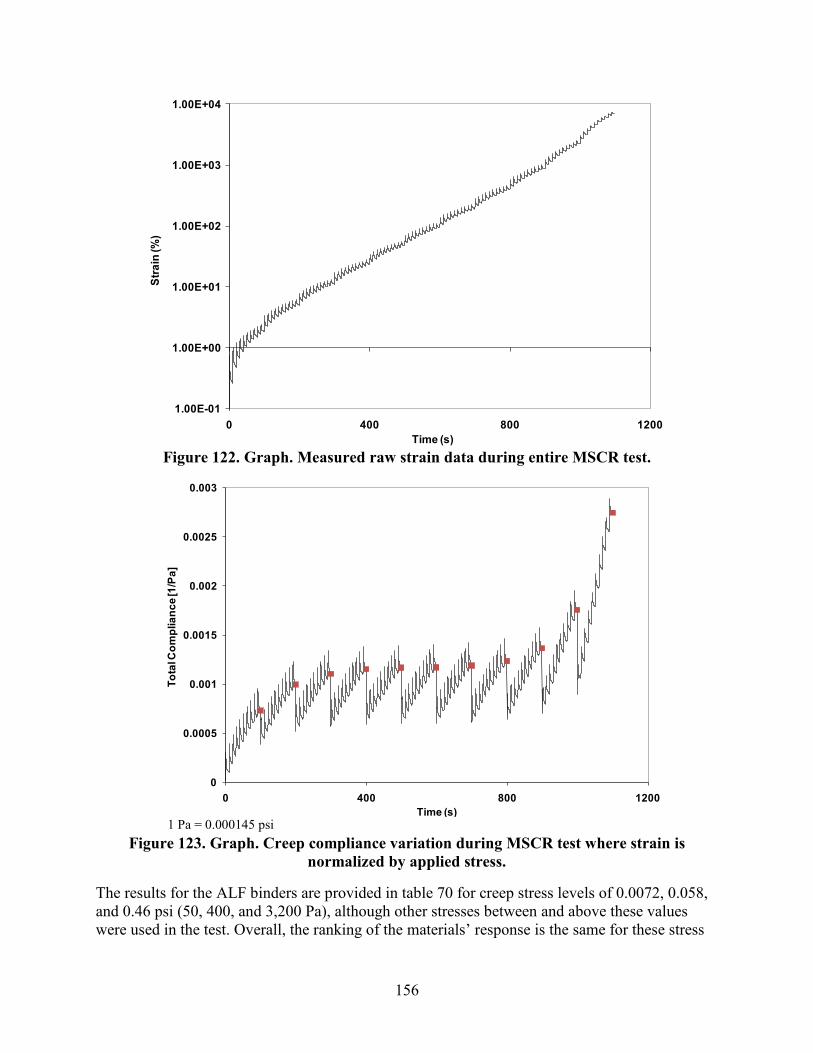
156

Figure 122. Graph. Measured raw strain data during entire MSCR test.

1 Pa = 0.000145 psi

Figure 123. Graph. Creep compliance variation during MSCR test where strain is normalized by applied stress.

The results for the ALF binders are provided in table 70 for creep stress levels of 0.0072, 0.058, and 0.46 psi (50, 400, and 3,200 Pa), although other stresses between and above these values were used in the test. Overall, the ranking of the materials’ response is the same for these stress

1.00E-01

1.00E+00

1.00E+01

1.00E+02

1.00E+03

1.00E+04

0 400 800 1200

Stra

in (%

)

Time (s)

0

0.0005

0.001

0.0015

0.002

0.0025

0.003

0 400 800 1200

Tota

l Com

plia

nce [

1/Pa

]

Time (s)

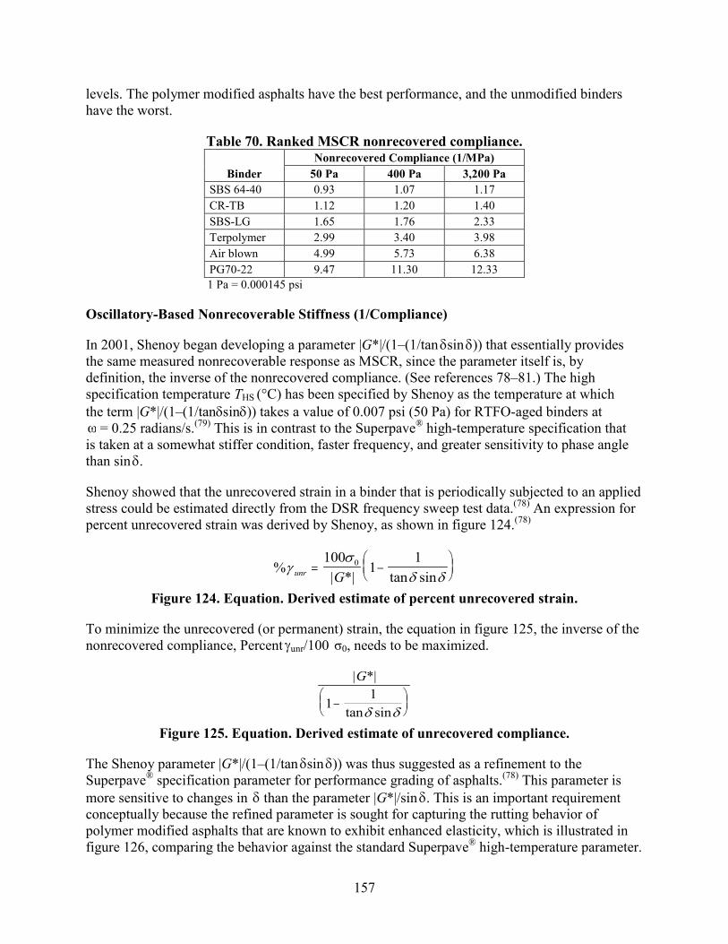
157

levels. The polymer modified asphalts have the best performance, and the unmodified binders have the worst.

Table 70. Ranked MSCR nonrecovered compliance.

Binder Nonrecovered Compliance (1/MPa)

50 Pa 400 Pa 3,200 Pa SBS 64-40 0.93 1.07 1.17 CR-TB 1.12 1.20 1.40 SBS-LG 1.65 1.76 2.33 Terpolymer 2.99 3.40 3.98 Air blown 4.99 5.73 6.38 PG70-22 9.47 11.30 12.33 1 Pa = 0.000145 psi

Oscillatory-Based Nonrecoverable Stiffness (1/Compliance)

In 2001, Shenoy began developing a parameter |G*|/(1–(1/tan sin )) that essentially provides the same measured nonrecoverable response as MSCR, since the parameter itself is, by definition, the inverse of the nonrecovered compliance. (See references 78–81.) The high specification temperature THS (°C) has been specified by Shenoy as the temperature at which the term |G*|/(1–(1/tanδsinδ)) takes a value of 0.007 psi (50 Pa) for RTFO-aged binders at

= 0.25 radians/s.(79) This is in contrast to the Superpave® high-temperature specification that is taken at a somewhat stiffer condition, faster frequency, and greater sensitivity to phase angle than sin .

Shenoy showed that the unrecovered strain in a binder that is periodically subjected to an applied stress could be estimated directly from the DSR frequency sweep test data.(78) An expression for percent unrecovered strain was derived by Shenoy, as shown in figure 124.(78)

%| *| tan sin

γσ

δ δunr G= −

1001

10

Figure 124. Equation. Derived estimate of percent unrecovered strain.

To minimize the unrecovered (or permanent) strain, the equation in figure 125, the inverse of the nonrecovered compliance, Percent unr/100 0, needs to be maximized.

| *|

tan sin

G

11

−

δ δ

Figure 125. Equation. Derived estimate of unrecovered compliance.

The Shenoy parameter |G*|/(1–(1/tan sin )) was thus suggested as a refinement to the Superpave® specification parameter for performance grading of asphalts.(78) This parameter is more sensitive to changes in than the parameter |G*|/sin . This is an important requirement conceptually because the refined parameter is sought for capturing the rutting behavior of polymer modified asphalts that are known to exhibit enhanced elasticity, which is illustrated in figure 126, comparing the behavior against the standard Superpave® high-temperature parameter.

δ δ

ω

δ

γ σ

δ δ

δ δ

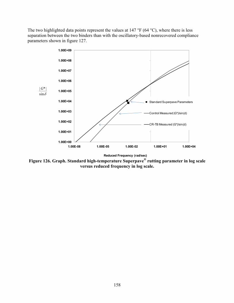
158

The two highlighted data points represent the values at 147 °F (64 °C), where there is less separation between the two binders than with the oscillatory-based nonrecovered compliance parameters shown in figure 127.

Figure 126. Graph. Standard high-temperature Superpave® rutting parameter in log scale

versus reduced frequency in log scale.

1.00E+00

1.00E+01

1.00E+02

1.00E+03

1.00E+04

1.00E+05

1.00E+06

1.00E+07

1.00E+08

1.00E+09

1.00E-08 1.00E-05 1.00E-02 1.00E+01 1.00E+04

and

Reduced Frequency (rad/sec)

Standard Superpave Parameters

Control Measured |G*|/sin(d)

CR-TB Measured |G*|/sin(d)

δsin|*| G

159

Figure 127. Graph. Oscillatory-based nonrecovered compliance rutting parameter in log

scale versus reduced frequency in log scale.

It was shown during the derivation of the Shenoy parameter |G*|/(1–(1/tan sin )) that the term (1 ‒ (1/tan sin )) tends to be zero at equal to about 52 degrees.(78) Hence, the parameter is rendered invalid at values of less than 52 degrees. During the course of the development of this parameter and the further development of the new criterion, when a host of binders were considered, it was found that less than 52 degrees was encountered in less than 1 percent of the total number of data points analyzed.(78,79) Since the |G*|/(1 ‒ (1/tan sin )) value is picked up at = 0.25 radians/s, it is virtually impossible (or rather the chances are very remote) to encounter less than 52 degrees. Even so, if one has to safeguard against any adverse situation and be prepared for the 0.1 percent chance, then one can use the fact that |G*|/(sin )9 (i.e., sinraised to the ninth power) is a close enough approximation, as proven earlier.(78) The parameter |G*|/(sin )9 can thus be used for less than 52 degrees. An if/then clause for the calculation using the formula “IF ( >55, |G*|/(1 – (1/tan sin )), |G*|/(sinδ)9)” in the Microsoft Excel® column does the job. Note that the cutoff value is taken to be 55 rather than 52 to be conservative. Using |G*|/(sin )9 as the refined parameter for all values of instead of |G*|/(1–(1/tan sin )) is not appropriate because |G*|/(sin )9 does not have any fundamental basis, while the parameter |G*|/(1 – (1/tan sin )) was derived using fundamental considerations. Figure 128 illustrates how a temperature grade in degrees Celsius can be determined using the Shenoy parameter with a recommended criterion of 0.0073 psi (50 Pa) in the same fashion as a temperature grade is determined with the current |G*|/sin parameter.

1.00E+00

1.00E+01

1.00E+02

1.00E+03

1.00E+04

1.00E+05

1.00E+06

1.00E+07

1.00E+08

1.00E+09

1.00E-08 1.00E-05 1.00E-02 1.00E+01 1.00E+04

and

Reduced Frequency (rad/sec)

CR-TB |G*|/[1-1/tan(d)sin(d)]

Control |G*|/[1-1/tan(d)sin(d)]

Modified Trigonometric Parameters

δδ sintan11

|*|

−

G

δ δ δ δ δ

δ

δ δ δ

ω δ

δ δ

δ δ δ δ δ

δ δ δ δ δ

δ δ

δ

160

°F = 1.8(°C) + 32

Figure 128. Graph. Oscillatory-based nonrecovered compliance rutting parameter in arithmetic scale versus temperature in log scale.

An alternative criterion was also suggested by Shenoy.(79,80) First an equi-stiffness temperature TE (°C) was defined as the temperature when |G*| takes a value of 0.0073 psi (50 Pa) for the RTFO-aged binder at = 0.25 radians/s, thereby taking care of the rheological contribution coming from one portion of the term |G*|/(1–(1/tan sin )). The contribution from the other portion was incorporated by dividing the equi-stiffness temperature TE (°C) by (1 – (1/tan sin )) using values at TE (°C). This resulted in the high specification temperature THS (°C) being defined as TE/(1 – (1/tan sin )). The sensitivity of the term 1/(1 – (1/tan sin )) compared to 1/sin is shown in figure 129. The increased sensitivity of the term 1/(1 – (1/tan sin )) to helps capture the elastic contribution of the modified asphalts in an enhanced manner compared to the term 1/sin .

Figure 129. Graph. Trigonometric functions for the standard high-temperature

Superpave® rutting parameters and oscillatory-based non-recovered compliance.

The ranked ALF binder properties from this technique are provided in table 71 for both the stiffness at the fixed temperature of 147 °F (64 °C) and the effective temperature. As previously described, the inverse of the modified trigonometric parameters is an estimate of the nonrecovered compliance derived from the theory. Figure 130 shows nonrecovered compliance from MSCR measurement with the nonrecovered compliance from the frequency sweep

ω δ δ

δ δ δ

δ δ δ δ δ δ δ δ

δ

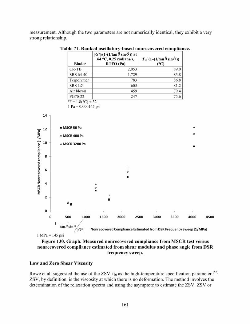
161

measurement. Although the two parameters are not numerically identical, they exhibit a very strong relationship.

Table 71. Ranked oscillatory-based nonrecovered compliance.

Binder

|G*|/(1-(1/tan sin )) at 64 °C, 0.25 radians/s,

RTFO (Pa) TE/ (1–(1/tan sin ))

(°C) CR-TB 2,053 89.0 SBS 64-40 1,729 83.8 Terpolymer 783 86.8 SBS-LG 605 81.2 Air blown 459 79.4 PG70-22 247 75.6

°F = 1.8(°C) + 32 1 Pa = 0.000145 psi

1 MPa = 145 psi

Figure 130. Graph. Measured nonrecovered compliance from MSCR test versus nonrecovered compliance estimated from shear modulus and phase angle from DSR

frequency sweep.

Low and Zero Shear Viscosity

Rowe et al. suggested the use of the ZSV 0 as the high-temperature specification parameter.(82) ZSV, by definition, is the viscosity at which there is no deformation. The method involves the determination of the relaxation spectra and using the asymptote to estimate the ZSV. ZSV or

δ δ δ δ

0

2

4

6

8

10

12

14

0 500 1000 1500 2000 2500 3000 3500 4000 4500

MSC

R N

onre

cove

red

com

plia

nce

[1/M

Pa]

Nonrecovered Compliance Estimated from DSR Frequency Sweep [1/MPa]

MSCR 50 Pa

MSCR 400 Pa

MSCR 3200 Pa

|*|sintan

11G

δδ−

η

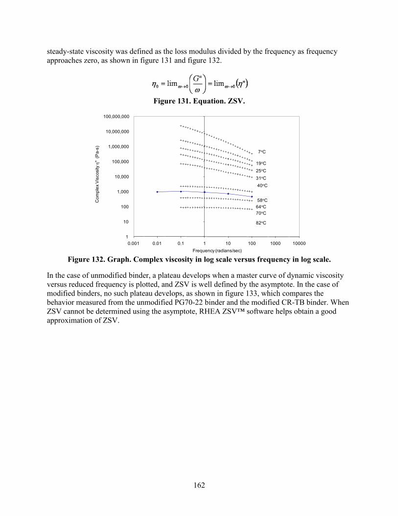
162

steady-state viscosity was defined as the loss modulus divided by the frequency as frequency approaches zero, as shown in figure 131 and figure 132.

Figure 131. Equation. ZSV.

Figure 132. Graph. Complex viscosity in log scale versus frequency in log scale.

In the case of unmodified binder, a plateau develops when a master curve of dynamic viscosity versus reduced frequency is plotted, and ZSV is well defined by the asymptote. In the case of modified binders, no such plateau develops, as shown in figure 133, which compares the behavior measured from the unmodified PG70-22 binder and the modified CR-TB binder. When ZSV cannot be determined using the asymptote, RHEA ZSV™ software helps obtain a good approximation of ZSV.

1

10

100

1,000

10,000

100,000

1,000,000

10,000,000

100,000,000

0.001 0.01 0.1 1 10 100 1000 10000

Com

plex

Vis

cosi

ty η

" (P

a-s)

Frequency (radians/sec)

7oC

31oC

19oC

58oC64oC70oC

82oC

25oC

40oC

163

Figure 133. Graph. Complex viscosity in log scale versus frequency in log scale.

Dongré et al. suggested the use of low shear viscosity (LSV) at a fixed frequency of 0.01 radians/s as the high-temperature specification parameter, as shown in figure 133 for the unmodified binder.(83,84) This parameter could be obtained directly from the experiment and did not need separate software for calculation as in the case of ZSV. The ZSV and LSV test results on the ALF binders are provided in table 72.

Table 72. Ranked ZSV and LSV. Binder ZSV (Pa-s) LSV (Pa-s)

CR-TB 9,302 7,183 SBS 64-40 7,791 7,660 SBS-LG 4,814 3,364 Terpolymer 2,974 2,470 Air blown 1,981 2,455 PG70-22 978 1,034

Material Volumetric Flow Rate

As a quick and easy method, Shenoy suggested the possibility of using the material’s volumetric-flow rate (MVR) as a high-temperature PG specification.(85,86) MVR is defined as the volume of the material (in milliliters or cubic centimeters) that is extruded in 10 min through a die of specific diameter and length by applying pressure through static weight load (L) under prescribed temperature conditions.

The MVR is determined through a closely defined flow measurement device (FMD) (see figure 134). This equipment is borrowed from the polymer industry, where it is routinely used to measure the melt flow index of polymers for purposes such as determining the suitability of polymer for blow injection molding. The equipment is less costly than by about a factor of 10 compared to dynamic shear rheometers. The cylinder of the FMD is made of hardened steel and is fitted with heaters, insulated, and controlled for operation at the required temperature. The heating device is capable of maintaining the temperature at 0.4 inches (10 mm) above the die to

164

within 0.4 °F (0.2 °C) of the desired temperature during the test. The temperature of the barrel from 0.4 to 2.9 inches (10 to 75 mm) above the top of the die is maintained within ±1 percent of the set temperature (°C) in strict compliance with ASTM D1238.(87) The piston is made of steel, and the diameter of its head is 0.0029 ±0.00058 inches (0.075 ±0.015 mm) less than that of the internal diameter of the cylinder, which is 0.37 inches (9.5 mm). Extrusion of the material is done through a die made of hardened steel with an internal diameter of 0.0817 ±0.0002 inches (2.095 ±0.005 mm).

Figure 134. Illustration. Key components of an FMD for determination of MVR.

MVR can be effectively used in determining the PG high-temperature specification. The method is straightforward, fast, and accurate. The high specification temperature THS (°C) has been specified by Shenoy as the temperature at which MVR takes a value of 50 cc/10 min for unaged binders when the imposed load on the sample forced out of a capillary is 2.697 lb (1.225 kg), as shown in figure 135.(85)

°F = 1.8(°C) + 32

Figure 135. Graph. MVR versus temperature.

MVR is easy to determine, and FMD that is used for the generation of MVR data is a relatively simple, inexpensive piece of equipment that can be carried from place to place because of its light weight. It neither needs arrangements for air pressure nor requires a circulating water bath to maintain a constant temperature environment. Since this equipment was originally built for taking polymer melt data at high temperatures (257–572 °F (125–300 °C)), it has an excellent temperature control system with variations of about 0.2 °F (0.1°C), especially in the temperature

LOAD

PISTON BARREL

HEATER ANDINSULATIONDIE

OPTICAL EYE

ASPHALT

165

range applicable to paving asphalts. It was found that MVR data generated from the FMD were highly reproducible.

Because FMD is relatively inexpensive, the operational costs are low, the MVR data generation requires minimal training, the output has low level of variability, no calibration is needed, and the equipment is portable, it merits its use at paving sites or refineries. The actual time for data generation is also very low. All this makes MVR an attractive parameter to be used for routine quality control as well as for new product development of asphalt binders and would serve as an excellent purchase guide specification for the users and producers of paving asphalts.

MVR and corresponding temperature grading of the ALF binders is provided in table 73. The unmodified binders have a high flow rate, but the softest, SBS 64-40, has the highest rate. The other polymer modified binders have the lowest rates, with SBS-LG and CR-TB having the smallest.

Table 73. Ranked MVR and temperature grade from FMD.

Binder MVR at 64 °C, 1.225 kg

(cc/10 min) Temperature at 50 cc/10 min,

1.225 kg (°C) SBS-LG 4.0 77.2 CR-TB 4.4 80.6 Terpolymer 6.1 81.2 PG70-22 11.7 73.5 Air blown 14.6 74.8 SBS 64-40 19.1 77.0

°F = 1.8(°C) + 32 1 kg = 2.202 lb

167

CHAPTER 6. MIXTURE PERFORMANCE TESTS

INTRODUCTION

A variety of material characterization tests were conducted on ALF cores, plant-produced mixtures, and laboratory-produced mixtures. This chapter describes both established characterization tests and methodologies that are undergoing development for future applications. Some tests provide a mechanistic engineering property, while others are an empirical qualitative assessment.

The mixture performance is primarily used in chapter 7 to accompany comparisons between binder properties and full-scale ALF performance. These cross-comparisons help capture the degree to which candidate binder parameters (discussed in chapter 5) can discriminate superiority or inferiority in expected performance. In contrast to comparisons between binder properties and full-scale ALF performance, these mixture characterization tests circumvent any influence from less-controlled construction and environmental/climatic variables present at ALF, essentially leveling the playing field by specifically emphasizing the binders’ contribution in a laboratory setting. Characterization of lab-produced mixtures provides more direct comparison to binder variables, especially when the air void content of the mixtures is a common fixed value. Characterization of core provides a more direct evaluation of mixture effects on the ALF performance.

The strengths of the various mixture characterization tests are evaluated at the end of this chapter using the statistical techniques described in chapter 3. Composite scores are calculated by comparing the laboratory results against the ALF rutting and cracking performance.

MIXTURE TESTS FOR RUTTING

HWT

HWT (AASHTO T 324) is a high-temperature, wet submerged test where a steel wheel is reciprocated over surfaces of HMA specimens to evaluate moisture damage and stripping of asphalt binder from the aggregate.(88) This pavement distress is outside the scope of this research. However, the test can also assess the permanent deformation characteristics via the rutting that is induced.

Plant-produced mixtures sampled during construction were compacted in a linear kneading compactor to produce slabs 12 inches (320 mm) long by 10 inches (260 mm) wide and 3 inches (80 mm) thick and having an air void content of 7 percent ±0.5 percent. The water temperature was brought to 147 °F (64 °C), the same temperature as the primary ALF rutting, instead of the cooler temperatures around 104–122 °F (40–50 °C) usually imposed in the test. Typical performance measured in the test is provided in figure 136, where rut depth is measured at individual numbers of cycles. Three replicates were tested, but a fourth was tested for the mixture from lane 6 to achieve a comparison to its corresponding mix in lane 12, and a fourth was tested for lane 8. The ALF mixtures’ performance is quantified by the number of cycles to achieve a 0.4-inch (10-mm) rut depth and is shown in table 74 and figure 137. There are no clear trends in terms of modified and unmodified binders. Performance of the same mixtures placed in

168

different lane thickness is, for the most part, comparable except for the control binder in lanes 2 and 8. Extracted binder contents of those tested specimens were explored between the two lanes and revealed no significant differences to raise concern. Additional HWT tests were conducted on laboratory-prepared materials with 0, 1 (job mix formula), and 1.5 percent hydrated lime to explore the effect of lime distribution and content given the aggregate stockpile dispersion problems described in table 11. The laboratory mixture with 0 percent lime exhibited 5,975 cycles to a 0.4-inch (10-mm) rut, similar to lane 8. The laboratory mixtures with 1.5 and 1.0 percent lime took 15,530 and 12,190 cycles to a 0.4-inch (10-mm) rut, respectively. This suggests that hydrated lime content in lane 8 was less than targeted, which is corroborated by table 11, where the measured lime content was less in lane 8 than in lane 2. The hypothesized net effect is that the lower lime content made the mix vulnerable to poorer than expected performance in this wet stripping test and possibly explains the discrepancy in table 74 and figure 137.

1 mm = 0.039 inches

Figure 136. Graph. HWT rut depth versus wheel tracking cycles.

Table 74. HWT performance of ALF mixtures.

Binder

Average Number of Passes to Reach 10-mm Rut Depth at 64 °C HMA from 100-mm ALF Sections HMA from 150-mm ALF Sections

Average Standard Deviation Average

Standard Deviation

CR-AZ 9,843 816 — — PG70-22 20,347 6,140 5,937 367 Air blown 14,900 2,025 14,092 1,983 SBS-LG 8,790 1,709 9,870 1,814 CR-TB 12,593 2,525 — — Terpolymer 9,277 2,738 6,977 934 Fiber 7,017 2,373 — — SBS 64-40 — — 5,137 483

°F = 1.8(°C) + 32 1 mm = 0.039 inches — Indicates test data were not measured.

0

5

10

15

20

25

0 5000 10000 15000 20000

Rut

Dep

th (m

m)

Wheel Tracking Cycles

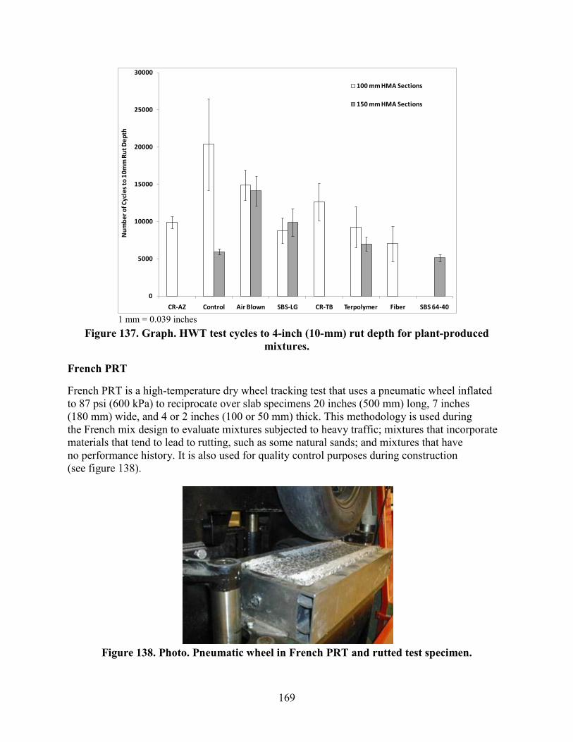
169

1 mm = 0.039 inches

Figure 137. Graph. HWT test cycles to 4-inch (10-mm) rut depth for plant-produced mixtures.

French PRT

French PRT is a high-temperature dry wheel tracking test that uses a pneumatic wheel inflated to 87 psi (600 kPa) to reciprocate over slab specimens 20 inches (500 mm) long, 7 inches (180 mm) wide, and 4 or 2 inches (100 or 50 mm) thick. This methodology is used during the French mix design to evaluate mixtures subjected to heavy traffic; mixtures that incorporate materials that tend to lead to rutting, such as some natural sands; and mixtures that have no performance history. It is also used for quality control purposes during construction (see figure 138).

Figure 138. Photo. Pneumatic wheel in French PRT and rutted test specimen.

0

5000

10000

15000

20000

25000

30000

CR-AZ Control Air Blown SBS-LG CR-TB Terpolymer Fiber SBS 64-40

Num

ber o

f Cyc

les t

o 10

mm

Rut

Dep

th

100 mm HMA Sections

150 mm HMA Sections

170

Plant-produced ALF mixtures were compacted to 4-inch (100-mm)-thick slabs at a target air void content of 7 percent ±0.5 percent. The test temperature was 165 °F (74 °C), and the rut depth was manually measured on the surface at 15 locations and averaged. Measurements were taken at 6,000, 20,000, and 60,000 cycles. Two replicate slabs were tested, and the results are summarized in table 75 and figure 139.

Table 75. Rut depths from French PRT.

Binder

Rut Depth at 60,000 Passes at 74 °C HMA from 100-mm ALF Sections HMA from 150-mm ALF Sections

Average (mm) Standard

Deviation (mm) Average (mm) Standard

Deviation (mm) CR-AZ 8.20 0.57 — — CR-AZ composite 14.30 0.99 — — Control (CR-AZ) 8.20 0.14 — — PG70-22 8.55 1.39 11.13 1.26 Air blown 8.00 0.42 8.20 1.84 SBS-LG 13.55 0.92 11.70 0.85 CR-TB 6.90 0.57 — — Terpolymer >20 — >20 — Fiber 15.10 1.70 — — SBS 64-40 — — >20 —

°F = 1.8(°C) + 32 1 mm = 0.039 inches — Indicates test data were not measured.

1 mm = 0.039 inches

Figure 139. Graph. Rut depth at 60,000 passes in French PRT for plant-produced mixtures.

0

2

4

6

8

10

12

14

16

18

20

CR-AZ CR-AZ Composite

Control (CR-AZ)

Control Air Blown SBS-LG CR-TB Terpolymer Fiber SBS 64-40

Fren

ch P

RT R

ut D

epth

at 6

0,00

0 Cy

cles

[mm

]

100mm HMA Sections

150mm HMA Sections

171

In general, variability was low. Like HWT, there is no clear trend with respect to modified and unmodified asphalt binders. The soft SBS 64-40 mixture and the terpolymer mixtures from both lanes exceeded the measurable rut depth of 0.8 inches (20 mm) at 60,000 cycles. The thickness of the slabs in this test allowed for composite slabs to reflect the structure of lane 1 CR-AZ/ PG70-22 in contrast to the thinner slabs in HWT, which do not allow composite slabs to be tested. The slabs with the lane 1 CR-AZ asphalt mixture on top of the PG70-22 mixture provided an average rut depth of 0.558 inches (14.3 mm). When tested by itself, the CR-AZ mixture provided a rut depth of 0.32 inches (8.2 mm). In contrast to the HWT performance, the control mixtures from lanes 2 and 8 were comparable, which strengthens the discussion that lime content differences were captured by the wet HWT. Although the lane 1 control mixture (underneath CR-AZ at ALF) was not tested by the French PRT at a slab thickness of 4 inches (100 mm), the same mixture from lane 2 only had a rut depth of 0.33 inches (8.6 mm). It was speculated that the higher rut depth for the two-layer system was the result of pockets of air voids being trapped between the two layers and of the discontinuity in aggregate structure.

SST RSCH

165 °F (74 °C) SST RSCH Lab-Compacted Plant-Produced Mix

RSCH tests were conducted in an SST, and permanent shear strain at 165 °F (74 °C) was measured following AASHTO TP 7-94.(89) A pulsed, haversine shear stress at a level of 10 psi (69.5 kPa) was applied to the test specimens from the horizontal actuator while the vertical actuator applied compression (or tension) to keep the height of the test sample constant. Plant-produced mix sampled from trucks during construction was compacted to 5.26-inch (135-mm)-tall specimens using the Superpave® gyratory compactor. Two specimens 2 inches (50 mm) tall were cut from each gyratory sample, and the target air void content of the final cut samples was 7 percent ±0.5 percent. The loading time was 0.1 s and the rest time was 0.6 s to allow recoverable strains to attenuate and thereby allow the nonrecoverable or permanent shear strain to be measured. The permanent shear strain grows nonlinearly, as shown in figure 140, which illustrates typical data from a less resistant lane 3 (air blown) and a more resistant lane 5 (CR-TB). Five replicates were tested. The tests were carried out until the shear strain limit of the machine was reached or 5,000 cycles.

172

Figure 140. Graph. Permanent shear strain in SST RSCH test versus number of load

cycles.

The performance of the ALF mixtures is quantified in table 76 and figure 141 by the number of cycles to reach 20,000 microstrains, equivalent to 2 percent strain. Variability was not consistent and could be either high or low. There is a general trend that the polymer modified binders perform better than the unmodified binders, except the gap-graded CR-AZ mixture. SBS-LG, PG70-22, air-blown, and terpolymer mixtures were placed in both the 4- and 5.8-inch (100- and 150-mm) thickness, and the laboratory performance of these mixtures is comparable, except for the terpolymer mixtures. The SST RSCH laboratory performance of lane 6 terpolymer is better than that of lane 12. This is opposite the French PRT, where the performance was comparable and poor.

Table 76. SST RSCH cycles to 2 percent permanent shear strain.

Binder

SST RSCH Cycles to Reach 2 Percent Permanent Shear Strain

100-mm HMA 150-mm HMA

Average Standard Deviation Average

Standard Deviation

CR-AZ 189 93 — — PG70-22 747 239 604 115 Air blown 537 59 520 39 SBS-LG 1212 324 1908 938 CR-TB 2089 734 — — Terpolymer 3141 1857 1642 365 Fiber 353 60 — — SBS 64-40 — — 765 825

1 mm = 0.039 inches — Indicates tests were not performed.

0

5000

10000

15000

20000

25000

30000

35000

40000

45000

0 500 1000 1500 2000 2500 3000 3500 4000 4500 5000

Perm

anen

t She

ar S

trai

n [m

icro

stra

in]

SST Shear Cycles

Air Blown Replicates

CR-TB Replicates

173

Figure 141. Graph. SST RSCH cycles to 2 percent permanent shear strain rut

for plant-produced mixtures.

147 °F (64 °C) SST RSCH ALF Cores

A full set of field cores from the thicker 5.8-inch (150-mm) ALF sections was taken in 2006, excluding lane 12 because ALF machines were located on top of the lane at the time. The field cores were split into top and bottom lifts and characterized at 147 °F (64 °C) rather than the 165 °F (74 °C) used for plant-produced mixtures. Three replicates were tested, but some lanes and lifts had only two replicates. Plots of the average permanent shear strain curves from the tests for the top and bottom lifts are shown in figure 142 and figure 143, respectively. As expected, there was little variation in the performance of these mixtures, but the general ranking was the same between top and bottom lifts. Table 77 and figure 144 show the average and standard deviation of number of cycles to 2 percent strain (20,000 microstrain) and the microstrain at 200 cycles.

0

1000

2000

3000

4000

5000

6000

CR-AZ Control Air Blown SBS-LG CR-TB Terpolymer Fiber SBS 64-40

Num

ber o

f RSC

H C

ycle

s to

2% P

erm

anen

t Str

ain

100 mm HMA Sections

150 mm HMA Sections

174

Figure 142. Graph. Permanent shear strain in SST RSCH test for top lifts versus

number of load cycles.

Figure 143. Graph. Permanent shear strain in SST RSCH test for bottom lifts

versus number of load cycles.

0

5000

10000

15000

20000

25000

30000

35000

0 200 400 600 800 1000 1200 1400

Perm

anen

t She

ar St

rain

(Mic

ro St

rain

)

Number of SST Cycles

Lane 8 Control Top

Lane 9 SBS 64-40 Top

Lane 10 Air Blown Top

Lane 11 Terpolymer Top

0

5000

10000

15000

20000

25000

30000

35000

0 200 400 600 800 1000 1200 1400

Perm

anen

t She

ar St

rain

(Mic

ro S

trai

n)

Number of SST Cycles

Lane 8 Control Bottom

Lane 9 SBS 64-40 Bottom

Lane 10 Air Blown Bottom

Lane 11 Terpolymer Bottom

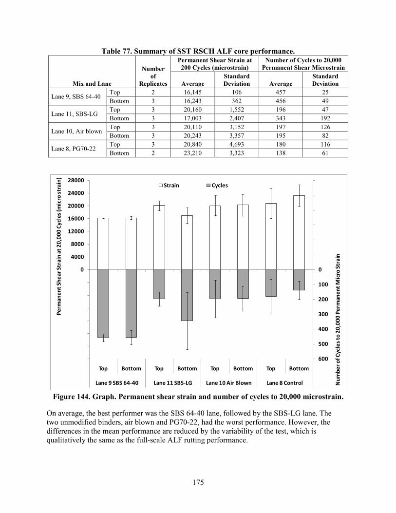
175

Table 77. Summary of SST RSCH ALF core performance.

Mix and Lane

Number of

Replicates

Permanent Shear Strain at 200 Cycles (microstrain)

Number of Cycles to 20,000 Permanent Shear Microstrain

Average Standard Deviation Average

Standard Deviation

Lane 9, SBS 64-40 Top 2 16,145 106 457 25 Bottom 3 16,243 362 456 49

Lane 11, SBS-LG Top 3 20,160 1,552 196 47 Bottom 3 17,003 2,407 343 192

Lane 10, Air blown Top 3 20,110 3,152 197 126 Bottom 3 20,243 3,357 195 82

Lane 8, PG70-22 Top 3 20,840 4,693 180 116 Bottom 2 23,210 3,323 138 61

Figure 144. Graph. Permanent shear strain and number of cycles to 20,000 microstrain.

On average, the best performer was the SBS 64-40 lane, followed by the SBS-LG lane. The two unmodified binders, air blown and PG70-22, had the worst performance. However, the differences in the mean performance are reduced by the variability of the test, which is qualitatively the same as the full-scale ALF rutting performance.

-600

-500

-400

-300

-200

-100

0

100

200

300

400

500

600-28000

-24000

-20000

-16000

-12000

-8000

-4000

0

4000

8000

12000

16000

20000

24000

28000

Top Bottom Top Bottom Top Bottom Top Bottom

Lane 9 SBS 64-40 Lane 11 SBS-LG Lane 10 Air Blown Lane 8 Control Num

ber o

f Cyc

les t

o 20

,000

Per

man

ent M

icro

Stra

in

Perm

anen

t She

ar St

rain

at 2

0,00

0 Cy

cles

(mic

ro st

rain

)

Strain Cycles

176

Dynamic Modulus |E*| and Phase Angle

Refer to chapter 4 section, “Direct Measurement of Asphalt Layer Modulus,” for a discussion of dynamic modulus measured on field cores, plant-produced mixtures, and laboratory- produced mixtures.

The dynamic modulus and phase angle from the plant-produced mixtures, lab-produced mixtures, and field cores are summarized at 66 and 136 °F (19 and 58 °C) both at 0.1 and 10 Hz. The 136 °F (58 °C) data are provided in this section, and the data at 66 °F (19 °C) pertaining to the ALF fatigue cracking tests are in the following section. Only cores from the thicker 5.8-inch (150-mm) lanes could be taken, and the plant-produced fiber mix was no longer available, so only the lab-produced mix is represented. Recall from chapter 4 that the effective frequency of the ALF wheel at various depths and temperatures was between 18 and 3.1 Hz. Although 136 °F (58 °C) was the highest practical temperature for dynamic modulus and is less than the 147 °F (64 °C) ALF rutting test, time-temperature superposition enables the behavior of the materials to be evaluated (see discussion of table 53 in chapter 4).

Cores are always softer than plant-produced and lab-produced mixtures, even though they are more dense (see table 78 and the discussion on compaction effects in chapter 4). The dynamic modulus and phase angle at 136 °F (58 °C) for 10 and 0.1 Hz are shown in table 79 and table 80, respectively. There is no clear trend where plant-produced mixtures are more or less stiff than their lab-produced counterparts.

Table 78. Air void content of dynamic modulus specimens.

Dynamic Modulus Specimens

Air Void Content (percent)

Plant-produced samples 7.0 ±0.5 Lab-produced samples 7.0 ±0.5

Cores

Lane 8, PG70-22 5.1 Lane 9, SBS 64-40 5.2 Lane 10, air blown 3.9 Lane 11, SBS-LG 5.3 Lane 12, terpolymer 4.5

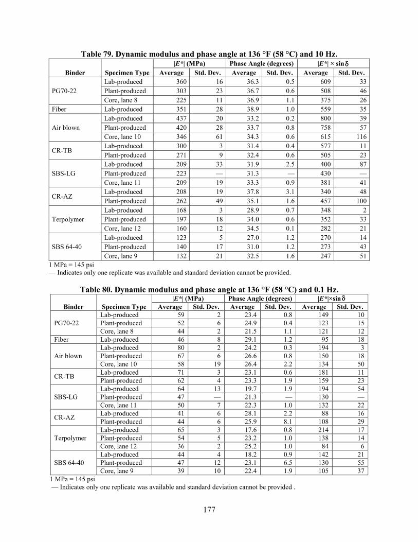
177

Table 79. Dynamic modulus and phase angle at 136 °F (58 °C) and 10 Hz.

Binder Specimen Type |E*| (MPa) Phase Angle (degrees) |E*| × sin

Average Std. Dev. Average Std. Dev. Average Std. Dev.

PG70-22 Lab-produced 360 16 36.3 0.5 609 33 Plant-produced 303 23 36.7 0.6 508 46 Core, lane 8 225 11 36.9 1.1 375 26

Fiber Lab-produced 351 28 38.9 1.0 559 35

Air blown Lab-produced 437 20 33.2 0.2 800 39 Plant-produced 420 28 33.7 0.8 758 57 Core, lane 10 346 61 34.3 0.6 615 116

CR-TB Lab-produced 300 3 31.4 0.4 577 11 Plant-produced 271 9 32.4 0.6 505 23

SBS-LG Lab-produced 209 33 31.9 2.5 400 87 Plant-produced 223 — 31.3 — 430 — Core, lane 11 209 19 33.3 0.9 381 41

CR-AZ Lab-produced 208 19 37.8 3.1 340 48 Plant-produced 262 49 35.1 1.6 457 100

Terpolymer Lab-produced 168 3 28.9 0.7 348 2 Plant-produced 197 18 34.0 0.6 352 33 Core, lane 12 160 12 34.5 0.1 282 21

SBS 64-40 Lab-produced 123 5 27.0 1.2 270 14 Plant-produced 140 17 31.0 1.2 273 43 Core, lane 9 132 21 32.5 1.6 247 51

1 MPa = 145 psi — Indicates only one replicate was available and standard deviation cannot be provided.

Table 80. Dynamic modulus and phase angle at 136 °F (58 °C) and 0.1 Hz.

Binder Specimen Type |E*| (MPa) Phase Angle (degrees) |E*|×sin

Average Std. Dev. Average Std. Dev. Average Std. Dev.

PG70-22 Lab-produced 59 2 23.4 0.8 149 10 Plant-produced 52 6 24.9 0.4 123 15 Core, lane 8 44 2 21.5 1.1 121 12

Fiber Lab-produced 46 8 29.1 1.2 95 18

Air blown Lab-produced 80 2 24.2 0.3 194 3 Plant-produced 67 6 26.6 0.8 150 18 Core, lane 10 58 19 26.4 2.2 134 50

CR-TB Lab-produced 71 3 23.1 0.6 181 11 Plant-produced 62 4 23.3 1.9 159 23

SBS-LG Lab-produced 64 13 19.7 1.9 194 54 Plant-produced 47 — 21.3 — 130 — Core, lane 11 50 7 22.3 1.0 132 22

CR-AZ Lab-produced 41 6 28.1 2.2 88 16 Plant-produced 44 6 25.9 8.1 108 29

Terpolymer Lab-produced 65 3 17.6 0.8 214 17 Plant-produced 54 5 23.2 1.0 138 14 Core, lane 12 36 2 25.2 1.0 84 6

SBS 64-40 Lab-produced 44 4 18.2 0.9 142 21 Plant-produced 47 12 23.1 6.5 130 55 Core, lane 9 39 10 22.4 1.9 105 37

1 MPa = 145 psi — Indicates only one replicate was available and standard deviation cannot be provided .

δ

δ

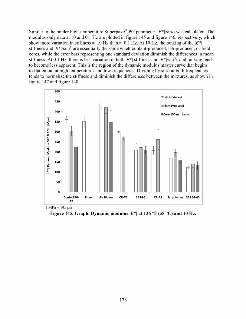
178

Similar to the binder high-temperature Superpave® PG parameter, |E*|/sin was calculated. The modulus-only data at 10 and 0.1 Hz are plotted in figure 145 and figure 146, respectively, which show more variation in stiffness at 10 Hz than at 0.1 Hz. At 10 Hz, the ranking of the |E*| stiffness and |E*|/sin are essentially the same whether plant-produced, lab-produced, or field cores, while the error bars representing one standard deviation diminish the differences in mean stiffness. At 0.1 Hz, there is less variation in both |E*| stiffness and |E*|/sin , and ranking tends to become less apparent. This is the region of the dynamic modulus master curve that begins to flatten out at high temperatures and low frequencies. Dividing by sin at both frequencies tends to normalize the stiffness and diminish the differences between the mixtures, as shown in figure 147 and figure 148.

1 MPa = 145 psi

Figure 145. Graph. Dynamic modulus |E*| at 136 °F (58 °C) and 10 Hz.

δ

δ

δ

δ

0

50

100

150

200

250

300

350

400

450

500

Control 70-22

Fiber Air Blown CR-TB SBS-LG CR-AZ Terpolymer SBS 64-40

|E*|

Dyn

amic

Mod

ulus

58C

& 1

0Hz [

Mpa

]

Lab Produced

Plant Produced

Core 150 mm Lanes

179

1 MPa = 145 psi

Figure 146. Graph. Dynamic modulus |E*| at 136 °F (58 °C) and 0.1 Hz.

1 MPa = 145 psi

Figure 147. Graph. |E*|/sin at 136 °F (58 °C) and 10 Hz.

0

10

20

30

40

50

60

70

80

90

Control 70-22

Fiber Air Blown CR-TB SBS-LG CR-AZ Terpolymer SBS 64-40

|E*|

Dyn

amic

Mod

ulus

58C

& 0

.1Hz

[Mpa

]

Lab Produced

Plant Produced

Core 150 mm Lanes

0

100

200

300

400

500

600

700

800

900

Control 70-22

Fiber Air Blown CR-TB SBS-LG CR-AZ Terpolymer SBS 64-40

|E*|

/Sin

(d) 5

8C &

10H

z [M

pa]

Lab Produced

Plant Produced

Core 150 mm Lanes

δ

180

1 MPa = 145 psi

Figure 148. Graph. |E*|/sin at 136 °F (58 °C) and 0.1 Hz.

Flow Number

Particular attention was paid to evaluating the performance of the ALF mixtures in AMPT (formerly SPT). This includes both dynamic modulus |E*| and flow number tests. AMPT was developed, in part, to overcome the challenges associated with the SST (cost of equipment, required expertise of technicians, pavement design framework, etc.), which was the recommended performance test equipment for the Superpave® system coming out of the SHRP research program. A further benefit of the flow number test is the application of the test results in mechanistic-empirical performance prediction of rutting using methodologies similar to those in the contemporary NCHRP 9-30A, Calibration of Rutting Models for HMA Structural and Mix Design.(90)

Like RSCH, the flow number test is a pulsed cyclic load and recovery test where the permanent strains are measured, but the loading is triaxial compression cycles repeatedly applied to cylindrical test specimens. Idealized behavior in the flow number test is shown in figure 149. Depending on the test conditions, the behavior can exhibit deformation in three regions. The first region is characterized by a large increase in permanent strain, the second region exhibits near linear growth of permanent strain, and the final region is marked by an inflection point and exhibits a more pronounced instability or tertiary flow.

0

50

100

150

200

250

300

Control 70-22

Fiber Air Blown CR-TB SBS-LG CR-AZ Terpolymer SBS 64-40

|E*|

/Sin

(d) 5

8C &

0.1

Hz [M

pa]

Lab Produced

Plant Produced

Core 150 mm Lanes

δ

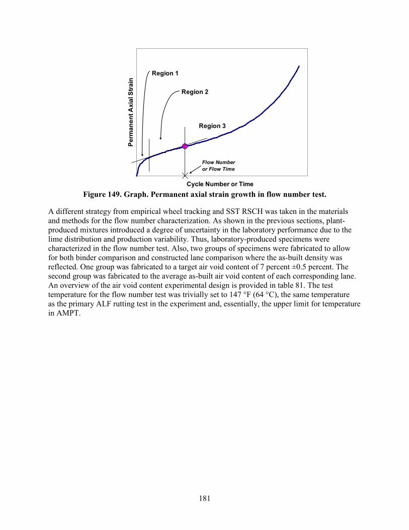
181

Figure 149. Graph. Permanent axial strain growth in flow number test.

A different strategy from empirical wheel tracking and SST RSCH was taken in the materials and methods for the flow number characterization. As shown in the previous sections, plant-produced mixtures introduced a degree of uncertainty in the laboratory performance due to the lime distribution and production variability. Thus, laboratory-produced specimens were characterized in the flow number test. Also, two groups of specimens were fabricated to allow for both binder comparison and constructed lane comparison where the as-built density was reflected. One group was fabricated to a target air void content of 7 percent ±0.5 percent. The second group was fabricated to the average as-built air void content of each corresponding lane. An overview of the air void content experimental design is provided in table 81. The test temperature for the flow number test was trivially set to 147 °F (64 °C), the same temperature as the primary ALF rutting test in the experiment and, essentially, the upper limit for temperature in AMPT.

Cycle Number or Time

Perm

anen

t Axi

al S

train

Region 1

Region 2

Region 3

Flow Number or Flow Time

182

Table 81. Summary of AMPT flow number test conditions.

Binder Type Corresponding

Test Lane Air Void Content

(percent)

Triaxial Stress Confining Pressure,

kPa (psi) Deviator Stress,

kPa (psi) PG70-22 PG70-22 + fiber Air blown CR-TB SBS-LG SBS 64-40 Terpolymer

General 7.00 69 (10) 523 (76)

PG70-22 100-mm lane 2 8.00

69 (10) 827 (120)

Air blown 100-mm lane 3 5.75 SBS-LG 100-mm lane 4 8.00 and 5.50 CR-TB 100-mm lane 5 7.75 and 5.25 Terpolymer 100-mm lane 6 7.60 PG70-22 + fiber 100-mm lane 7 8.00 PG70-22 150-mm lane 8 5.00

6.9 (1) and 69 kPa (10)

207 (30) and 827 (120)

SBS 64-40 150-mm lane 9 4.14 Air blown 150-mm lane 10 5.50 SBS-LG 150-mm lane 11 5.43 Terpolymer 150-mm lane 12 5.85

1 mm = 0.039 inches

Less guidance and application for the flow number test is in practice compared to the established dynamic modulus |E*| stiffness characterization test. As a consequence, the flow number test has been performed with a lack of consensus on stress state and temperature. However, the FHWA Asphalt Mixtures ETG organized a group from industry, agencies, and academia to develop further guidance, an ongoing process at the time this report was written. Depending on the choice of the triaxial stress state and temperature, the flow number test could last a very long time, even without the occurrence of the tertiary flow. Therefore, understanding the mechanism of permanent deformation in asphalt materials and determining the factors that influence the outcomes of the flow number test is an important priority for the research community.

Recently, Gibson et al. developed a more complete understanding of the mechanism of permanent deformation in AC and provided mechanistic-based recommendations for appropriate triaxial stress states for the flow number test.(91) Fully mechanistic, constitutive material models for viscoplasticity (time- and temperature-dependent permanent strains) were used to assess multiaxial stress states that are induced within asphalt layers under truck tires to identify critical locations that yield significantly more deformation than others. Some locations had stress states with larger equivalent deviator stress, which would tend produce larger permanent strains, but equivalent confining stresses in those regions were also larger and tended to reduce the amount of permanent strain from the corresponding deviator stress. Conversely, some locations had smaller equivalent deviator stresses that would produce smaller permanent strains but also had smaller equivalent confining stresses, thereby increasing the amount of permanent strains due to the corresponding deviator stress. The analysis yielded a critical location under the edge of tires a few inches deep, as shown in figure 150.

183

Figure 150. Illustration. Calculated volumetric permanent strains in a vertical cross

sectional plane in the direction of vehicle travel.

A representative equivalent triaxial compression stress state in this region was found to be 10 psi (69 kPa) confinement and 76 psi (523 kPa) axial deviator stress. This stress state was used in the first group of ALF mixtures, with the same 7 percent air void content for all binders, but did not produce a flow number (tertiary flow inflection) within 20,000 cycles. The deviator stress was increased to 120 psi (827 kPa) for the second group of ALF mixtures fabricated to the as-built density of their corresponding lanes in hopes of producing tertiary flow but did not. In addition, the five ALF mixtures prepared for the 5.8-inch (150-mm) HMA sections were tested with a second stress state that was essentially unconfined but with less deviator stress based on estimates from the analysis previously described. Unconfined tests are more convenient given that latex rubber membranes around the specimens are not needed. Gibson et al. includes more discussion on specialty radial strain measurement equipment used in experiments that required a very small (1 psi (7 kPa)) positive confining stress in the essentially unconfined test.(91) Regardless, all tests produced usable permanent deformation curves, even though tertiary flow was only observed in a few mixtures.

Three replicates were tested at each condition. Plots of the average permanent deformation curves for the different mixtures and stress states are provided in figure 151 through figure 153. These data are further reduced in table 82, which quantifies the permanent strain at a fixed number of cycles depending on the test conditions, shown graphically in figure 154 through figure 156.

184

Figure 151. Graph. Axial permanent strain versus number of cycles for mixes with

7 percent air void content, 10 psi (69 kPa) confinement, and 76 psi (523 kPa) axial deviator stress.

Figure 152. Graph. Axial permanent strain versus number of cycles for mixes with as-built air void content, 10 psi (69 kPa) confinement, and 120 psi (827 kPa) axial deviator stress.

185

Figure 153. Graph. Axial permanent strain versus number of cycles for mixes with as-built

air void content, 1 psi (6.9 kPa) confinement, and 30 psi (207 kPa) axial deviator stress.

Table 82. AMPT flow number performance.

Binder

Permanent Strain at 20,000 Cycles, 7 Percent

Air Void Content Permanent Strain at 5,000 Cycles Fabricated to As-Built Air Void Content 69 kPa confinement/

523 kPa axial deviator stress

69 kPa confinement/827 kPa axial deviator stress 6.9 kPa confinement/

207 kPa axial deviator stress 100-mm ALF Sections 150-mm ALF Sections 150-mm ALF Sections (only)

Average Standard Deviation Average

Standard Deviation Average

Standard Deviation Average

Standard Deviation

PG70-22 49,303 6,450 64,340 12,196 49,615 10,355 20,138 2,470 Air blown 33,741 3,782 40,260 8,804 36,576 7,249 12,391 566

SBS-LG 30,421 3,890 49,773 6,761

28,814 6,639 10,274 2,070 30,429 2,228

CR-TB 38,420 12,662 44,071 2,736

— — — — 19,965 2,001 Terpolymer 22,145 2,741 39,096 9,748 21,504 1,767 7,209 603 Fiber 34,061 1,713 45,558 3,192 — — — — SBS 64-40 46,210 3,477 — — 25,076 13,960 7,365 3,610 1 kPa = 0.145 psi 1 mm = 0.039 inches — Indicates tests were not performed.

186

Figure 154. Graph. Permanent axial microstrain at 20,000 cycles for ALF mixtures with

7 percent air voids at 10 psi (69 kPa) confinement and 76 psi (523 kPa) axial deviator stress.

Figure 155. Graph. Permanent axial microstrain at 5,000 cycles for 4-inch (100-mm)

ALF mixtures with as-built air void content at 10 psi (69 kPa) confinement and 120 psi (827 kPa) axial deviator stress.

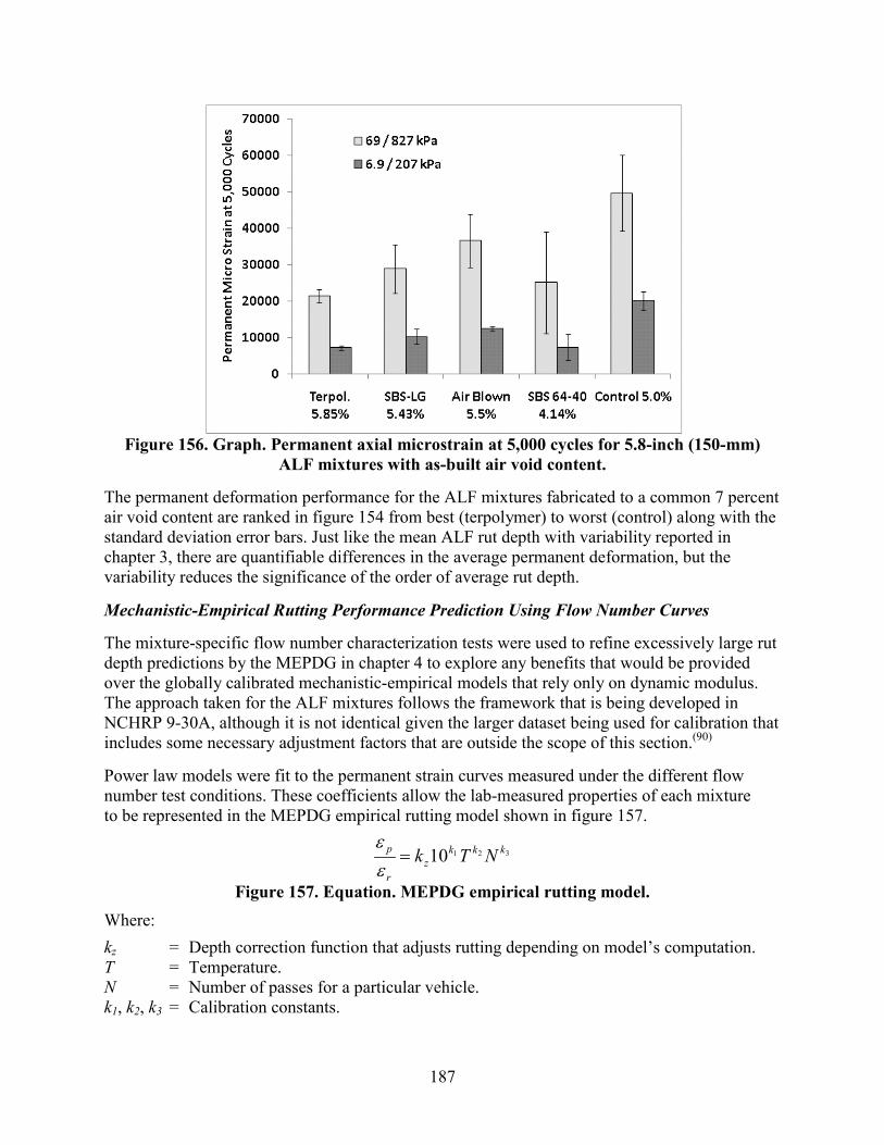
187

Figure 156. Graph. Permanent axial microstrain at 5,000 cycles for 5.8-inch (150-mm)

ALF mixtures with as-built air void content.

The permanent deformation performance for the ALF mixtures fabricated to a common 7 percent air void content are ranked in figure 154 from best (terpolymer) to worst (control) along with the standard deviation error bars. Just like the mean ALF rut depth with variability reported in chapter 3, there are quantifiable differences in the average permanent deformation, but the variability reduces the significance of the order of average rut depth.

Mechanistic-Empirical Rutting Performance Prediction Using Flow Number Curves

The mixture-specific flow number characterization tests were used to refine excessively large rut depth predictions by the MEPDG in chapter 4 to explore any benefits that would be provided over the globally calibrated mechanistic-empirical models that rely only on dynamic modulus. The approach taken for the ALF mixtures follows the framework that is being developed in NCHRP 9-30A, although it is not identical given the larger dataset being used for calibration that includes some necessary adjustment factors that are outside the scope of this section.(90)

Power law models were fit to the permanent strain curves measured under the different flow number test conditions. These coefficients allow the lab-measured properties of each mixture to be represented in the MEPDG empirical rutting model shown in figure 157.

Figure 157. Equation. MEPDG empirical rutting model.

Where: kz = Depth correction function that adjusts rutting depending on model’s computation. T = Temperature. N = Number of passes for a particular vehicle. k1, k2, k3 = Calibration constants.

32110 kkkz

r

p NTk=εε

188

Elastic recoverable strain, R, from mechanistic primary response calculations in the MEPDG is used to compute a corresponding plastic irrecoverable strain, P, by means of the ratio between these two strains in figure 157 rearranged in figure 158.

Figure 158. Equation. Plastic irrecoverable strain.

First, the strain ratio, which can be found specifically from laboratory tests, is equated to the same ratio that is used in the MEPDG (see figure 159). Figure 160 illustrates how the power law form that represents the laboratory flow number test is substituted for P in figure 159.

Figure 159. Equation. Equivalence assumed between laboratory performance and MEPDG

mechanistic-empirical model formulation.

Figure 160. Equation. Equating laboratory test power law permanent deformation

parameters with MEPDG mechanistic-empirical model formulation.

Next, it is necessary to produce the equivalent laboratory-based recoverable strain from the lab test in figure 160 using the dynamic modulus master curves of the mixtures and the deviator stresses applied in the flow number tests, as shown in figure 161.

Figure 161. Equation. Derivation of recoverable strain for MEDPG mechanistic-empirical permanent deformation model based on applied stress in flow number test and dynamic

modulus.

The dynamic modulus of HMA is sensitive to confining pressure as well as to other variables. Thus, the unconfined dynamic modulus would not be entirely appropriate to use in figure 161 when the confined flow number tests are being used in this approach. Kim et al. quantified the sensitivity of dynamic modulus to confining pressure, as shown in figure 162, where modulus increases in the high-temperature, low-frequency region of the dynamic modulus master curve.(92) Based on this data, it was assumed that dynamic modulus increases by a factor of 2 at 147 °F (64 °C) and frequency is equivalent to the load pulse in the flow number test.

ε ε

32110 kkkzrp NTk×= εε

ε

MEPDGr

p

LabTestr

p

=

εε

εε

32110 kkkz

LabTestr

b

NTkaN=

ε

|*| Erσε =

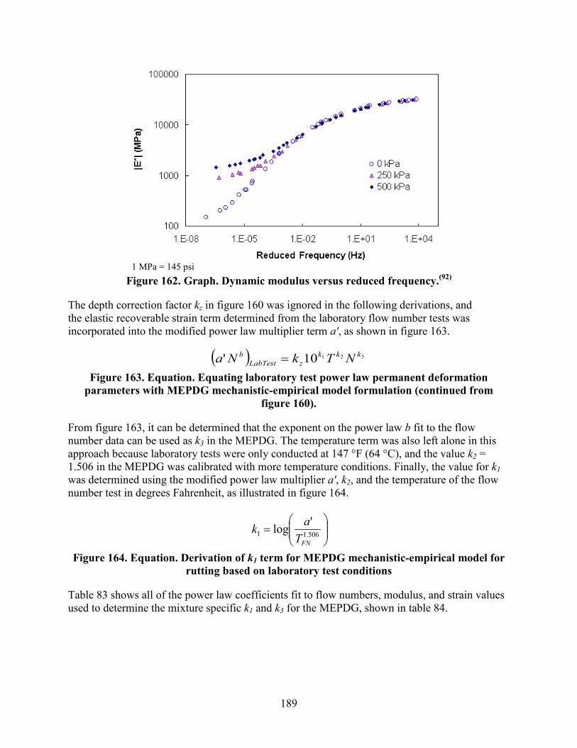
189

1 MPa = 145 psi

Figure 162. Graph. Dynamic modulus versus reduced frequency.(92)

The depth correction factor kz in figure 160 was ignored in the following derivations, and the elastic recoverable strain term determined from the laboratory flow number tests was incorporated into the modified power law multiplier term a', as shown in figure 163.

Figure 163. Equation. Equating laboratory test power law permanent deformation

parameters with MEPDG mechanistic-empirical model formulation (continued from figure 160).

From figure 163, it can be determined that the exponent on the power law b fit to the flow number data can be used as k3 in the MEPDG. The temperature term was also left alone in this approach because laboratory tests were only conducted at 147 °F (64 °C), and the value k2 = 1.506 in the MEPDG was calibrated with more temperature conditions. Finally, the value for k1 was determined using the modified power law multiplier a', k2, and the temperature of the flow number test in degrees Fahrenheit, as illustrated in figure 164.

Figure 164. Equation. Derivation of k1 term for MEPDG mechanistic-empirical model for

rutting based on laboratory test conditions

Table 83 shows all of the power law coefficients fit to flow numbers, modulus, and strain values used to determine the mixture specific k1 and k3 for the MEPDG, shown in table 84.

( ) 32110' kkkzLabTest

b NTkNa =

= 506.11

'logFNTak

190

Table 83. Modulus, recoverable strain, and permanent strain curve power law coefficients for mix-specific MEPDG rutting predictions

Mix

64 °C Modulus

(kPa)

Recoverable Strain (microstrain)

Power Law Coefficients Fit to Flow Number Data 69/827 kPa 6.9/207 kPa

6.9 kPa Confinement

69 kPa Confinement a b a b

Lane 2 180,594 1,146 2,290 1329.9 0.446 — — Lane 3 253,465 817 1,631 2920.7 0.309 — — Lane 4 164,323 1,260 2,516 3106.6 0.265 — — Lane 5 365,015 567 1,133 2730.9 0.320 — — Lane 6 125,926 1,644 3,284 4181.0 0.253 — — Lane 8 192,150 1,077 2,152 2228.4 0.358 803.9968 0.385196 Lane 9 125,802 1,645 3,287 3463.6 0.258 1638.743 0.225394 Lane 10 293,289 706 1,410 2464.8 0.323 551.3707 0.397649 Lane 11 181,215 1,142 2,282 3920.9 0.226 1568.197 0.219232 Lane 12 145,914 1,419 2,834 4565.6 0.185 2500.387 0.144622

°F = 1.8(°C) + 32 1 kPa = 0.145 psi — Indicates tests were not conducted.

Table 84. Mixture-specific MEPDG rutting model coefficients.

Mix

Coefficients determined from 69/827 kPa tests

Coefficients determined from 6.9/207 kPa tests

k1 k2 k3 k1 k2 k3 Lane 2 -3.620 1.5606 0.4465 — — — Lane 3 -3.130 1.5606 0.3093 — — — Lane 4 -3.293 1.5606 0.2651 — — — Lane 5 -3.001 1.5606 0.3196 — — — Lane 6 -3.279 1.5606 0.2530 — — — Lane 8 -3.366 1.5606 0.3580 -3.508 1.5606 0.385 Lane 9 -3.362 1.5606 0.2582 -3.383 1.5606 0.225 Lane 10 -3.140 1.5606 0.3226 -3.4917 1.5606 0.398 Lane 11 -3.148 1.5606 0.2262 -3.247 1.5606 0.219 Lane 12 -3.176 1.5606 0.1853 -3.138 1.5606 0.145

1 kPa = 0.145 psi — Indicates tests were not conducted Note: MEPDG global calibration values: k1 = -3.354 , k2 = 1.506, and k3 = 0.479.

The same standalone version of the MEPDG described in chapter 4 was used to compute the rut depths of the ALF lanes using the mixture-specific coefficients calibrated to the laboratory flow number tests. The rut depths for the following conditions were predicted:

• 147 °F (64 °C) rutting in all lanes, no wheel wander.

• 165 °F (74 °C) rutting in the 4-inch (100-mm) lanes, no wheel wander.

• 113 °F (45 °C) rutting in 5.8-inch (150-mm) lanes, no wheel wander.

• 66 °F (19 °C) rutting that occurred during fatigue testing in all lanes with wheel wander.

191

Figure 165 illustrates the best and worst rut depth predictions of the 4-inch (100-mm) ALF lanes using 10 psi (69 kPa) confined flow number tests. Figure 166 illustrates the best and worst rut depth predictions of the 5.8-inch (150 mm) ALF lanes using 1 psi (6.9 kPa) confined flow number tests. The magnitudes of the predicted rutting at 147 °F (64 °C) are significantly improved when compared to the predicted values in figure 82 from the MEPDG using global calibrations. Most predictions at 147 °F (64 °C) match well, and only one in figure 165 was mediocre. The rutting predictions of the 113 °F (45 °C) ALF tests are shown in figure 167 and were all under-predicted by about one-half. Predictions of the 66 °F (19 °C) rut depths were much smaller than the measured values and predictions of the 165 °F (74 °C) rut depths were much larger. Figure 168 and figure 169 are cross-plots of measured versus predicted rutting at two distinct passes: one point during the beginning of loading and one toward the end of loading. Predictions from all temperatures using the 10 and 1 psi (69 and 6.9 kPa) flow number data are shown in figure 168 and figure 169, respectively. These figures illustrate that more practical, less confined flow number tests can provide comparable predictions to more confined tests so long as the deviator stresses are adjusted accordingly. Rut depth predictions at temperatures warmer than the laboratory characterization were over-predicted and vice-versa. These results also suggest rutting predictions using the framework previously described could be improved using flow number tests at more than one temperature to better capture the temperature term. Nonetheless, this analysis illustrates the value of using mixture-specific inputs in the MEPDG rutting framework that NCHRP 9-30A is pursuing.(90)

1 mm = 0.039 inches

Figure 165. Graph. Rut depth versus number of ALF passes for best and worst 4-inch (100-mm) ALF lanes.

0

5

10

15

20

25

0 10000 20000 30000 40000 50000 60000

Rut

Dep

th, m

m

ALF Passes

Lane2-Measured

Lane2-Predicted

Lane4-Measured

Lane4-Predicted

192

1 mm = 0.039 inches

Figure 166. Graph. Rut depth versus number of ALF passes for best and worst 5.8-inch (150-mm) ALF lanes.

1 mm = 0.039 inches

Figure 167. Graph. Rut depth versus number of ALF passes for 113 °F (45 °C) ALF tests.

0

5

10

15

20

25

0 5000 10000 15000 20000 25000 30000 35000 40000 45000 50000

Rut

Dep

th, m

m

ALF Passes

Lane8-Measured

Lane8-Predicted

Lane10-Measured

Lane10-Predicted

0

1

2

3

4

5

6

7

8

9

10

0 50,000 100,000 150,000 200,000 250,000 300,000 350,000 400,000

Rut

Dep

th, m

m

ALF Passes

Lane8-Measured

Lane8-Predicted

Lane10-Measured

Lane10-Predicted

Lane11-Measured

Lane11-Predicted

193

1 mm = 0.039 inches

Figure 168. Graph. Predicted rutting in log scale versus measured rutting in log scale using 10 psi (69 kPa) confined flow number test data at 147 °F (64 °C).

1 mm = 0.039 inches

Figure 169. Graph. Predicted rutting in log scale versus measured rutting in log scale using 1 psi (6.9 kPa) confined flow number test data at 147 °F (64 °C).

0.01

0.1

1

10

100

1 10 100

Pred

icte

d Ru

t Dep

th, m

m

Measured Rut Depth, mm

74C

64C

45C

19C

0.01

0.1

1

10

100

1 10 100

Pred

icte

d Ru

t Dep

th, m

m

Measured Rut Depth, mm

64C

45C

19C

194

MIXTURE TESTS FOR FATIGUE CRACKING

Texas Transportation Institute Overlay Tester

Zhou et al. described a characterization methodology developed at the Texas Transportation Institute (TTI) originally intended to characterize the reflection crack resistance of HMA overlay composite specimens capable of including geosynthetic.(93) A schematic of the overlay tester (OT) is shown in figure 1701, where an HMA specimen is bonded between a fixed plate and moveable plate with a 0.08-inch (2-mm) gap that opens and closes to simulate the movements of underlying joints or cracks. The opening and closing is computer-controlled in a cyclic manner where the magnitude of the opening displacement is 0.025 inches (0.63 mm) in a triangular waveform lasting 10 s and then repeated. In addition to characterizing reflection crack resistance, Zhou et al. proposed that the methodology can potentially be used to screen mixtures for fatigue crack resistance.(93)

1 mm = 0.039 inches

Figure 170. Illustration. Side view of OT showing fixed and moveable horizontal plates.(93)

ALF cores were taken from the 4-inch (100-mm) test sections and shared with TTI staff for OT characterization in early 2006. The number of cycles to fully propagate a crack through the field cores was measured at 66 °F (19 °C) and a cyclic opening displacement of 0.019 inches (0.48 mm). The results provided in table 85 show polymer modified binders are more resistant than unmodified binders. The fiber mixture was eventually tested and required 110 cycles to failure, which is inconsistent with the fatigue-resistant performance under ALF. This is perplexing but is also corroborated by axial cyclic fatigue tests not being able to reflect the beneficial aspects of the fiber modification but still being able to capture the fatigue resistance from polymer modification.

Table 85. ALF 4-inch (100-mm) field core performance in TTI OT.(93)

Binder Number of Cycles to Full

Fracture in TTI OT Lane 2, PG70-22 60 Lane 3, air blown 80 Lane 4, SBS-LG 1,890 Lane 5, CR-TB 890 Lane 6, terpolymer 1,120

1Permission is given with the understanding that none of the material will be used to imply Transportation Research Board, AASHTO, or FHWA endorsement of a particular product, method, or practice.

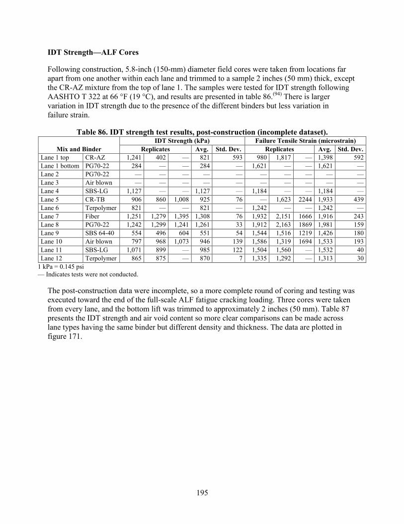
195

IDT Strength—ALF Cores

Following construction, 5.8-inch (150-mm) diameter field cores were taken from locations far apart from one another within each lane and trimmed to a sample 2 inches (50 mm) thick, except the CR-AZ mixture from the top of lane 1. The samples were tested for IDT strength following AASHTO T 322 at 66 °F (19 °C), and results are presented in table 86.(94) There is larger variation in IDT strength due to the presence of the different binders but less variation in failure strain.

Table 86. IDT strength test results, post-construction (incomplete dataset).

Mix and Binder IDT Strength (kPa) Failure Tensile Strain (microstrain)

Replicates Avg. Std. Dev. Replicates Avg. Std. Dev. Lane 1 top CR-AZ 1,241 402 — 821 593 980 1,817 — 1,398 592 Lane 1 bottom PG70-22 284 — — 284 — 1,621 — — 1,621 — Lane 2 PG70-22 — — — — — — — — — — Lane 3 Air blown — — — — — — — — — — Lane 4 SBS-LG 1,127 — — 1,127 — 1,184 — — 1,184 — Lane 5 CR-TB 906 860 1,008 925 76 — 1,623 2244 1,933 439 Lane 6 Terpolymer 821 — — 821 — 1,242 — — 1,242 — Lane 7 Fiber 1,251 1,279 1,395 1,308 76 1,932 2,151 1666 1,916 243 Lane 8 PG70-22 1,242 1,299 1,241 1,261 33 1,912 2,163 1869 1,981 159 Lane 9 SBS 64-40 554 496 604 551 54 1,544 1,516 1219 1,426 180 Lane 10 Air blown 797 968 1,073 946 139 1,586 1,319 1694 1,533 193 Lane 11 SBS-LG 1,071 899 — 985 122 1,504 1,560 — 1,532 40 Lane 12 Terpolymer 865 875 — 870 7 1,335 1,292 — 1,313 30

1 kPa = 0.145 psi — Indicates tests were not conducted.

The post-construction data were incomplete, so a more complete round of coring and testing was executed toward the end of the full-scale ALF fatigue cracking loading. Three cores were taken from every lane, and the bottom lift was trimmed to approximately 2 inches (50 mm). Table 87 presents the IDT strength and air void content so more clear comparisons can be made across lane types having the same binder but different density and thickness. The data are plotted in figure 171.

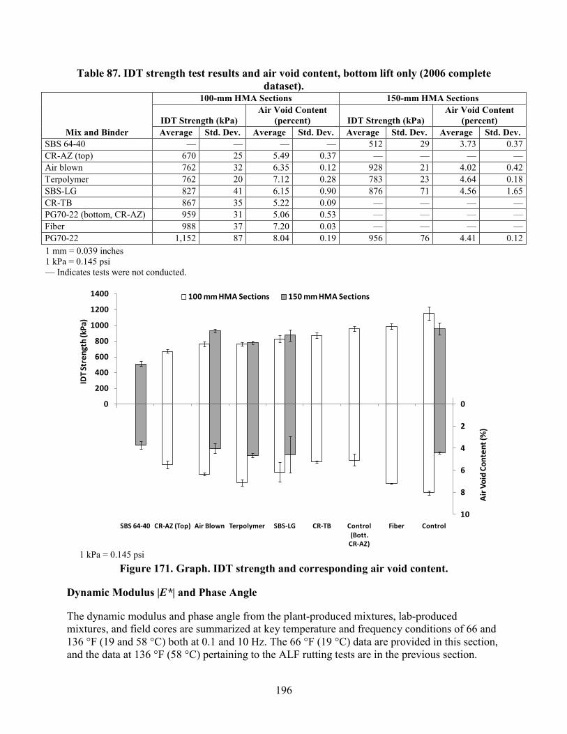
196

Table 87. IDT strength test results and air void content, bottom lift only (2006 complete dataset).

Mix and Binder

100-mm HMA Sections 150-mm HMA Sections

IDT Strength (kPa) Air Void Content

(percent) IDT Strength (kPa) Air Void Content

(percent) Average Std. Dev. Average Std. Dev. Average Std. Dev. Average Std. Dev.

SBS 64-40 — — — — 512 29 3.73 0.37 CR-AZ (top) 670 25 5.49 0.37 — — — — Air blown 762 32 6.35 0.12 928 21 4.02 0.42 Terpolymer 762 20 7.12 0.28 783 23 4.64 0.18 SBS-LG 827 41 6.15 0.90 876 71 4.56 1.65 CR-TB 867 35 5.22 0.09 — — — — PG70-22 (bottom, CR-AZ) 959 31 5.06 0.53 — — — — Fiber 988 37 7.20 0.03 — — — — PG70-22 1,152 87 8.04 0.19 956 76 4.41 0.12 1 mm = 0.039 inches 1 kPa = 0.145 psi — Indicates tests were not conducted.

1 kPa = 0.145 psi

Figure 171. Graph. IDT strength and corresponding air void content.

Dynamic Modulus |E*| and Phase Angle

The dynamic modulus and phase angle from the plant-produced mixtures, lab-produced mixtures, and field cores are summarized at key temperature and frequency conditions of 66 and 136 °F (19 and 58 °C) both at 0.1 and 10 Hz. The 66 °F (19 °C) data are provided in this section, and the data at 136 °F (58 °C) pertaining to the ALF rutting tests are in the previous section.

-10

-8

-6

-4

-2

0

2

4

6

8

10-1400

-1200

-1000

-800

-600

-400

-200

0

200

400

600

800

1000

1200

1400

SBS 64-40 CR-AZ (Top) Air Blown Terpolymer SBS-LG CR-TB Control (Bott.

CR-AZ)

Fiber Control

Air

Void

Con

tent

(%)

IDT

Stre

ngth

(kPa

)

100 mm HMA Sections 150 mm HMA Sections

197

Only cores from the 5.8-inch (150-mm) lanes could be taken and plant-produced fiber mix was no longer available, so only lab-produced mix is represented. Recall from chapter 4 that the effective frequency of the ALF wheel at various depth and temperatures was found between 18 and 3.1 Hz. The temperature of these laboratory tests matched the 66 °F (19 °C) ALF fatigue cracking test.

The dynamic modulus and phase angle at 66 °F (19 °C) for 10 and 0.1 Hz are shown in table 88 and table 89, respectively. Contrary to the 136 °F (58 °C) tests, there is no strong trend as to the denser cores being softer or stiffer than the gyratory-compacted specimens. There is also no strong trend where plant-produced mixtures are more or less stiff than the lab-produced counterparts. The |E*|×sin is calculated similar to the binder intermediate Superpave® PG specification parameter. The modulus-only data at 10 and 0.1 Hz are plotted in figure 172 and figure 173 respectively, with both showing variation in stiffness. The |E*|/sin loss modulus data at 10 and 0.1 Hz are plotted in figure 174 and figure 175. The ranking of the |E*| stiffness and |E*|/sin are essentially the same whether plant-produced, lab-produced, or field cores, while the error bars representing one standard deviation diminish the differences in mean stiffness. Multiplying by sin at both frequencies tends to normalize the stiffness and diminish the differences between the mixtures.

Table 88. Dynamic modulus and phase angle at 66 °F (19 °C) and 10 Hz.

Binder Specimen Type |E*| (MPa) Phase Angle (degrees) |E*|×sin

Average Std. Dev. Average Std. Dev. Average Std. Dev.

PG70-22 Lab-produced 7,847 515 19.4 0.4 2,605 134 Plant-produced 7,226 635 19.8 0.4 2,447 174 Core, lane 8 6,531 208 23.4 0.2 2,593 98

Fiber Lab-produced 7,864 428 19.3 0.0 2,601 138

Air blown Lab-produced 6,561 842 20.2 0.4 2,265 262 Plant-produced 6,518 697 20.5 0.2 2,279 224 Core, lane 10 6,068 1101 22.4 0.2 2,313 424

CR-TB Lab-produced 4,536 162 22.1 0.2 1,708 47 Plant-produced 4,347 74 23.9 1.0 1,759 52

SBS-LG Lab-produced 4,467 113 25.4 0.7 1,912 33 Plant-produced 3,591 1406 27.6 4.1 1,463 525 Core, lane 11 4,766 579 25.2 0.4 2,028 217

CR-AZ Lab-produced 4,251 424 28.1 1.4 1,996 123 Plant-produced 4,168 327 23.7 0.5 1,675 101

Terpolymer Lab-produced 3,726 217 29.6 0.4 1,839 84 Plant-produced 4,126 378 26.5 0.3 1,843 155 Core, lane 12 4,268 231 29.2 1.1 2,078 74

SBS 64-40 Lab-produced 1,723 216 32.9 1.6 931 86 Plant-produced 2,694 133 30.6 0.2 1,371 61 Core, lane 9 2,355 99 32.0 0.2 1,247 53

1 MPa = 145 psi

δ

δ

δ

δ

δ

198

Table 89. Dynamic modulus and phase angle at 66 °F (19 °C) and 0.1 Hz.

Binder Specimen Type |E*| (MPa) Phase Angle (degrees) |E*|×sin

Average Std. Dev. Average Std. Dev. Average Std. Dev.

PG70-22 Lab-produced 2,211 171 31.0 0.5 1,140 72 Plant-produced 2,059 152 31.0 0.3 1,059 69 Core, lane 8 1,553 20 34.4 1.0 878 31

Fiber Lab-produced 2,271 89 31.7 0.4 1,192 48

Air blown Lab-produced 1,997 188 27.9 0.3 936 81 Plant-produced 1,927 182 29.0 0.1 934 87 Core, lane 10 1,709 348 29.0 0.6 827 158

CR-TB Lab-produced 1,353 30 27.8 0.0 630 14 Plant-produced 1,202 68 30.3 1.0 605 17

SBS-LG Lab-produced 962 62 31.9 0.9 508 22 Plant-produced 789 368 31.7 1.0 361 197 Core, lane 11 1,096 133 33.0 0.6 596 63

CR-AZ Lab-produced 1,022 129 32.8 1.6 553 77 Plant-produced 1,060 99 31.2 1.0 548 39

Terpolymer Lab-produced 660 58 31.7 0.2 347 29 Plant-produced 931 106 30.8 0.3 477 51 Core, lane 12 795 104 34.8 0.7 453 51

SBS 64-40 Lab-produced 324 36 30.7 0.6 165 18 Plant-produced 516 30 31.2 0.2 268 15 Core, lane 9 478 31 31.7 0.7 251 14

1 MPa = 145 psi

1 MPa = 145 psi

Figure 172. Graph. Dynamic modulus |E*| at 66 °F (19 °C) and 10 Hz.

δ

0

1000

2000

3000

4000

5000

6000

7000

8000

9000

Control 70-22

Fiber Air Blown CR-TB SBS-LG CR-AZ Terpolymer SBS 64-40

|E*|

Dyn

amic

Mod

ulus

19C

& 1

0Hz [

Mpa

]

Lab Produced

Plant Produced

Core 150 mm Lanes

199

1 MPa = 145 psi

Figure 173. Graph. Dynamic modulus |E*| at 66 °F (19 °C) and 0.1 Hz.

1 MPa = 145 psi

Figure 174. Graph. |E*|sin at 66 °F (19 °C) and 10 Hz.

0

500

1000

1500

2000

2500

3000

Control 70-22

Fiber Air Blown CR-TB SBS-LG CR-AZ Terpolymer SBS 64-40

|E*|

Dyn

amic

Mod

ulus

19C

& 0

.1Hz

[Mpa

]

Lab Produced

Plant Produced

Core 150 mm Lanes

0

500

1000

1500

2000

2500

3000

Control 70-22

Fiber Air Blown CR-TB SBS-LG CR-AZ Terpolymer SBS 64-40

|E*|

xSin

(d) 1

9C &

10H

z [M

pa]

Lab Produced

Plant Produced

Core 150 mm Lanes

δ

200

1 MPa = 145 psi

Figure 175. Graph. |E*|sin at 66 °F (19 °C) and 0.1 Hz.

Axial Cyclic Fatigue

Few conventional flexural beam fatigue tests (AASHTO TP 8) were conducted before equipment malfunctions forced the laboratory to pursue alternate methodologies.(95) Several research tasks within NCHRP 9-19 developed advanced, fully mechanistic models for AC, giving a comprehensive description of permanent deformation and cracking.(96) A large portion of the NCHRP 9-19 advanced models’ framework was based on viscoelastic continuum damage (VECD) theories that describe the manner in which small microcracks develop, coalesce, and grow into macrocracks.(97,98) Research has shown contemporary VECD for asphalt offers several advantages.(92) The primary advantage is the utilization of a single damage characteristic curve, which can be calibrated using less effort in the laboratory than classical beam fatigue tests. VECD test specimens can be fabricated in the Superpave® gyratory compactor. Once the damage characteristic curve is found, it can theoretically be used to describe the damage and cracking response at any temperature and under any generalized inputs whether stress-control or strain-control, cyclic or monotonic, or random. The reader is encouraged to explore the literature cited in this section to observe the predictive capabilities that show that the theory and experimental evidence agree quite well.

Rigorously complete VECD has been used to develop methodologies for multiple cycle fatigue tests with the advantages previously described but with more practicality from less mathematical and computational overhead and decreased laboratory characterization burden. (See references 92, 96, 97, and 99–103.) Another significant advantage of this approach is the characteristics of the specimen geometry, stresses, strains, and temperatures make it able to be integrated into

0

200

400

600

800

1000

1200

1400

Control 70-22

Fiber Air Blown CR-TB SBS-LG CR-AZ Terpolymer SBS 64-40

|E*|

xSin

(d) 1

9C &

0.1

Hz [M

pa]

Lab Produced

Plant Produced

Core 150 mm Lanes

δ

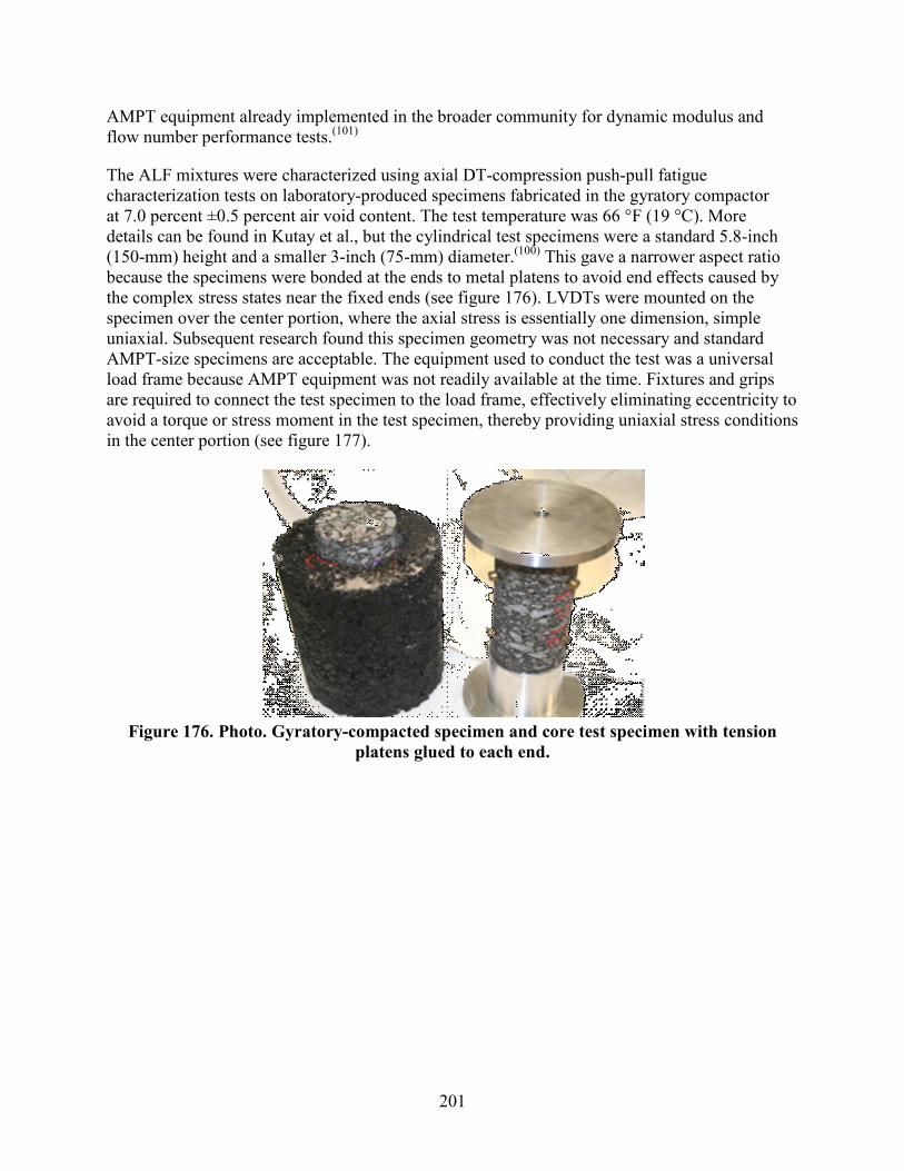
201

AMPT equipment already implemented in the broader community for dynamic modulus and flow number performance tests.(101)

The ALF mixtures were characterized using axial DT-compression push-pull fatigue characterization tests on laboratory-produced specimens fabricated in the gyratory compactor at 7.0 percent ±0.5 percent air void content. The test temperature was 66 °F (19 °C). More details can be found in Kutay et al., but the cylindrical test specimens were a standard 5.8-inch (150-mm) height and a smaller 3-inch (75-mm) diameter.(100) This gave a narrower aspect ratio because the specimens were bonded at the ends to metal platens to avoid end effects caused by the complex stress states near the fixed ends (see figure 176). LVDTs were mounted on the specimen over the center portion, where the axial stress is essentially one dimension, simple uniaxial. Subsequent research found this specimen geometry was not necessary and standard AMPT-size specimens are acceptable. The equipment used to conduct the test was a universal load frame because AMPT equipment was not readily available at the time. Fixtures and grips are required to connect the test specimen to the load frame, effectively eliminating eccentricity to avoid a torque or stress moment in the test specimen, thereby providing uniaxial stress conditions in the center portion (see figure 177).

Figure 176. Photo. Gyratory-compacted specimen and core test specimen with tension

platens glued to each end.

202

Figure 177. Photo. Instrumented tension mounted in universal test machine.

Two types of sinusoidal loading at 10 Hz were used: stress control and actuator strain control. The stress-controlled tests applied a zero-mean stress where the magnitude of the applied peak stress (in both tension and compression states) was 88 psi (610 kPa) or peak-to-peak 177 psi (1,220 kPa). The average predicted tensile stresses at the bottom of the ALF HMA were 312.2 and 208.4 psi (2,153 and 1,437 kPa) for the 4- and 5.8-inch (100- and 150-mm) ALF lanes, respectively. It may be inferred that the actual tensile stresses were larger. However, the applied stress level in the laboratory provided reasonable test duration and was of a relevant order of magnitude. Table 90 summarizes the initial strains measured in the stress-controlled tests. Healing characteristics of the modified and unmodified binders were also characterized in the stress-controlled tests. Rest periods of 10 and 30 min were allowed at the 1,000th and 6,000th cycles, respectively. After that, the loading continued until failure. The analysis clearly showed that healing characteristics of polymer modified binders such as the SBS-LG, terpolymer, and CR-TB were more pronounced (better) than those of PG70-22, air blown, and fiber. The polymer modified binders regained more stiffness after the rest period than the unmodified binders.

Table 90. Initial strain levels of ALF mixtures in stress-controlled fatigue tests.

Mixture Initial LVDT Strain in Stress-

Control Tests (microstrain) Fiber 93 SBS-LG 208 Terpolymer 265 CR-TB 202 PG70-22 105 Air blown 124 SBS 64-40 722

During the displacement-controlled tests, the strain level at the actuator or the platen-to-platen strain was controlled instead of the on-specimen mounted LVDT strain ( lvdt). This was chosen because the actuator may easily become unstable and apply very high loads for a fraction of a second, possibly damaging the specimen and other LVDTs if the test was controlled by an

ε

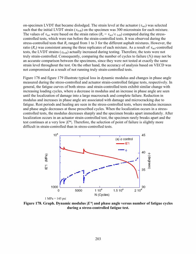
203

on-specimen LVDT that became dislodged. The strain level at the actuator ( act) was selected such that the initial LVDT strain ( lvdt) on the specimen was 300 microstrain for each mixture. The values of act were based on the strain ratios (Rε = act/ lvdt) computed during the stress-controlled tests, which were run before the strain-controlled tests. It was observed during the stress-controlled tests that Rε ranged from 1 to 3 for the different asphalt mixtures. However, the ratio (Rε) was consistent among the three replicates of each mixture. As a result of act-controlled tests, the LVDT strains ( lvdt) actually increased during testing. Therefore, the tests were not truly strain-controlled. Consequently, comparing the number of cycles to failure (Nf) may not be an accurate comparison between the specimens, since they were not tested at exactly the same strain level throughout the test. On the other hand, the accuracy of analysis based on VECD was not compromised as a result of not running truly strain-controlled tests.

Figure 178 and figure 179 illustrate typical loss in dynamic modulus and changes in phase angle measured during the stress-controlled and actuator strain-controlled fatigue tests, respectively. In general, the fatigue curves of both stress- and strain-controlled tests exhibit similar change with increasing loading cycles, where a decrease in modulus and an increase in phase angle are seen until the localization of damage into a large macrocrack and complete failure. Reduction in modulus and increases in phase angle are associated with damage and microcracking due to fatigue. Rest periods and healing are seen in the stress-controlled tests, where modulus increases and phase angle decreases at those prescribed cycles. When the localization occurs in a stress-controlled tests, the modulus decreases sharply and the specimen breaks apart immediately. After localization occurs in an actuator strain-controlled test, the specimen rarely breaks apart and the test continues at a very low |E*|. Therefore, the selection of point of failure is slightly more difficult in strain-controlled than in stress-controlled tests.

1 MPa = 145 psi

Figure 178. Graph. Dynamic modulus |E*| and phase angle versus number of fatigue cycles during a stress-controlled fatigue test.

ε ε

ε ε ε

ε ε

204

1 MPa = 145 psi

Figure 179. Graph. Dynamic modulus |E*| and phase angle versus number of fatigue cycles during a strain-controlled fatigue test.

Several different fatigue failure criteria were identified based on historical asphalt fatigue research summarized by Kutay et al.(100) The simplest definition of failure is the point where half of the initial modulus is lost. Other methodologies consider dissipated energy lost due to damage. The energy ratio (R) in figure 180 and dissipated energy ratio (DER) in figure 181 (from figure 182) quantify the manner in which fatigue damage is dissipated from cycle to cycle in such fatigue tests. This is similar to the foundation for the Superpave® intermediate-temperature fatigue cracking parameter, |G*|×sin , described in chapter 1.

Figure 180. Equation. Energy ratio.

Figure 181. Equation. DER.

Figure 182. Equation. Calculation of dissipated energy from phase angle, stress, and strain.

Where:

N = Number of cycles. Winitial = Dissipated strain energy computed at the first cycle. WN = Dissipated strain energy computed at cycle N. WN+1 = Dissipated strain energy computed at cycle N+1.

oN = Peak stress measured at the Nth cycle.

oN = Peak strain measured at the Nth cycle.

N = Phase angle measured at the Nth cycle.

δ

R = Winitial * N

WN

DER = WN+1 – WN

WN

WN = π σ0N ε0

N sin(ϕN)

σ ε φ

205

In stress-controlled tests, the failure point is defined when R is at its peak value. However, in strain-controlled tests, the R versus N relationship is linear, and the failure point is defined when the curve sharply deviates from a linear line. The failure point based on the DER is taken where the DER sharply increases from a plateau value.

When stress and strain of viscoelastic materials, such as AC, are plotted together, an oval- shaped hysteresis loop is observed due to the phase lag between stress and strain. The area within this hysteresis loop is proportional to the dissipated strain energy. Fatigue failure was also identified by quantifying the quality of the hysteresis loop. In specimens with growing damage microcracking (no macrocracks), the hysteresis loop changes but is still smooth. However, when a fracture or macrocrack has occurred, the shape of the hysteresis loop becomes distorted. The standard error from best-fit curves to the measured sinusoidal stress and strain was calculated and failure was taken as the point where this value jumps from the baseline during the test.

Table 91 summarizes the fatigue life of the ALF mixtures based on the various definitions of failure in both the stress-controlled and actuator strain-controlled tests. Failure from the different criteria is generally close to each other under stress-controlled tests, and the ranking does not change with different criteria. However, there was a wider variation in fatigue life from the strain-controlled tests, and the 50 percent reduction in |E*| criterion in general showed failure occurring sooner than the energy ratios and hysteresis loop distortion. Stiff mixtures performed better in stress-controlled tests and softer mixtures performed better in strain-controlled tests. The softest mixture, SBS 64-40, failed very fast in stress-controlled tests. In strain control, the SBS 64-40 mixture lost modulus very early but then exhibited a nearly flat curve, which resulted in no discernable trends for the energy ratios or hysteresis loops. In stiff mixtures, initial observed strains resulting from the applied load level in the stress-controlled tests were much lower than the initial 300 microstrain that was used in the actuator strain-controlled tests (see table 90). As a result, the number of cycles to failure for the stiff mixtures in stress-controlled tests was much higher than in strain-controlled tests. Conversely, initial strains at the soft mixtures resulting from the same load level were much higher than those of stiff mixtures; as a result, they failed quickly at the stress-controlled tests. Most importantly, table 91 shows a reversal in ranking depending on the mode of control, which is similar to what was observed in the binder tests described in chapter 5.

Table 91. Number of cycles to fatigue failure from different failure criteria.

Mixture

Energy Ratio Dissipated Energy

Ratio Hysteresis Loop

Distortion 50 Percent Modulus Reduction

Control ACT

Control

Control ACT

Control

Control ACT

Control

Control ACT

Control Control VECD

SBS 64-40 900 N/A 883 N/A 833 N/A 370 33,100 5,071,587 Terpolymer 3,893 128,250 4,659 133,450 5,243 127,800 2,660 88,500 1,333,521 CR-TB 5,560 31,434 6,659 31,068 6,933 31,601 2,510 6,168 59,655 SBS LG 4,893 14,500 5,942 13,567 8,393 13,367 4,333 1,875 167,880 Air blown 18,093 3,050 17,926 2,675 23,093 2,833 15,760 2,150 11,855 Fiber 50,593 1,063 60,093 1,000 63,926 1,000 44,426 1,000 25,119 PG70-22 25,093 750 28,260 688 31,426 563 24,593 438 12,589 N/A = Not available.

σ ε σ ε σ ε σ ε ε

206

The last column in table 91 provides the fatigue life using VECD principles based on damage characteristic curves to compute fatigue life idealized in truly strain-controlled conditions (see details in Kutay et al.).(100) This methodology provides a correction for the transient on-specimen strains in the actuator strain-controlled tests. In other words, the VECD approach allows a somewhat faster but significantly more practical actuator strain-controlled test to determine the inherent fatigue properties, which are then used to predict the fatigue life as if the test was conducted in strain control over the center portion of the test specimen. The ranking between the actuator strain-controlled tests and the VECD true strain-controlled computations changes slightly, but the unmodified binders are still less fatigue-resistant than the modified binders. For the group mixes in the 4-inch (100-mm)-thick ALF lanes, the fiber mix is better than the control binder and the air blown mixture is the worst performer. The terpolymer binder is still the best but with significantly larger fatigue life, and the SBS-LG binder is now better than the CR-TB binder.

The laboratory performance of the fiber mixture is particularly perplexing in both stress- and strain-controlled testing and does not reflect the high level of fatigue cracking resistance observed in ALF. This is also corroborated by the TTI OT. In stress-controlled testing, the performance closer to the stiffer unmodified binders exhibited better fatigue resistance. In strain-controlled testing, the fiber mixture performed worse, like the unmodified binders. Additional research is needed to explain why this performance is not captured in the laboratory.

Mixture EWF and Calculated CTOD

Asphalt mixtures can be characterized using the same methodologies as binder for EWF and CTOD properties because of the relative simplicity of the specimen geometry and loading. DENT specimens were 4.41 inches tall by 3.31 inches wide by 2.02 inches thick (113 mm tall by 85 mm wide by 52 mm thick) and cut from Superpave® gyratory compactor specimens made to 7 percent ±0.5 percent air void content. The ligament lengths were between 4 and 1.4 inches (100 and 35 mm). Figure 183 shows a test specimen. The temperature and displacement rates were 66 °F (19 °C) at 0.02 inches/min (0.5 mm/min).

207

Figure 183. Photo. Asphalt mixture DENT specimen for EWF and CTOD characterization.

Tests were conducted at five ligament lengths, each with two replicates. An example of the fracture energy dependence on ligament length from the air-blown mixture is shown in figure 184, which is comparable to the binder characteristic plotted in figure 115. Mixtures with modified asphalt binders indicate better performance than unmodified binders for both EWF and CTOD. The fiber mixture was tested, but the fracture energy results at the different ligament lengths were very erratic. The overall repeatability of the test on mixtures is less than desirable for an implementable, routine test. At least 10 specimens have to be tested for a reliable number, although there is a trade-off between number of replicates and number of ligament lengths. Nonetheless, the relevance of the binder-based version of EWF and CTOD tests is reinforced because there is an agreeable ranking between the binder properties and mixture properties, as shown in table 92. Binder EWF is about 10 times that of mixture, and binder CTOD is about 20 times that of mixture.

208

1 kJ/m2 = 23,730 lb-ft2/s2

1 mm = 0.0309 inches Figure 184. Graph. Fracture energy versus ligament length from mixture DENT testing.

Table 92. EWF and CTOD properties of asphalt aggregate mixtures.

Mixture EWF (kJ/m2) CTOD (mm)

Binder Mix Binder Mix SBS-LG 10.8 1.02 24.0 1.25 Terpolymer 4.70 0.85 15.7 1.14 CR-TB 4.40 0.60 8.5 0.57 PG70-22 7.90 0.97 7.5 0.71 Air blown 7.80 0.70 6.8 0.55

1 kJ/m2 = 23,730 lb-ft2/s2 1 mm = 0.039 inches

EVALUATION OF MIXTURE TESTS’ ABILITY TO DISCRIMINATE PERFORMANCE

The performance of the ALF mixtures in the laboratory are compared to the full-scale ALF performance using the composite statistical scoring outlined in chapter 3. Mixture tests that have the strongest indicator of ALF performance (highest correct composite score) are identified so as to narrow down one test for permanent deformation and fatigue cracking for use in chapter 7, where the individual binder parameters are compared against both full-scale ALF performance and laboratory mixture performance.

Rutting and Permanent Deformation

Comparisons for rutting are particularly challenging given the similarities in rut depth of the ALF lanes and the notable anomalous performance of lane 6 (terpolymer). Table 93 lists the laboratory tests and conditions that are compared to ALF rut depth at 25,000 passes and also identifies whether the trend should be proportional or inverse.

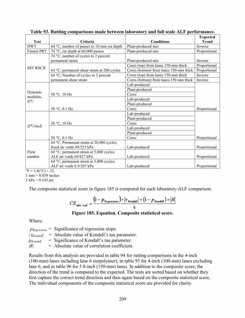
209

Table 93. Rutting comparisons made between laboratory and full scale ALF performance.

Test Criteria Conditions Expected

Trend HWT 64 °C; number of passes to 10-mm rut depth Plant-produced mix Inverse French PRT 74 °C; rut depth at 60,000 passes Plant-produced mix Proportional

SST RSCH

74 °C; number of cycles to 2 percent permanent strain Plant-produced mix Inverse

64 °C; permanent shear strain at 200 cycles Cores (top) from lanes 150-mm thick Proportional Cores (bottom) from lanes 150-mm thick Proportional

64 °C; Number of cycles to 2 percent permanent shear strain

Cores (top) from lanes 150-mm thick Inverse Cores (bottom) from lanes 150 mm thick Inverse

Dynamic modulus, |E*|

58 °C, 10 Hz

Lab-produced

Proportional

Plant-produced Cores

58 °C, 0.1 Hz

Lab-produced Plant-produced Cores

|E*|/sin 58 °C, 10 Hz

Lab-produced

Proportional

Plant-produced Cores

58 °C, 0.1 Hz

Lab-produced Plant-produced Cores

Flow number

64 °C; Permanent strain at 20,000 cycles; fixed air voids 69/523 kPa Lab-produced Proportional 64 °C; permanent strain at 5,000 cycles; ALF air voids 69/827 kPa Lab-produced Proportional 64 °C; permanent strain at 5,000 cycles; ALF air voids 6.9/207 kPa Lab-produced Proportional

°F = 1.8(°C) + 32 1 mm = 0.039 inches 1 kPa = 0.145 psi

The composite statistical score in figure 185 is computed for each laboratory-ALF comparison.

Figure 185. Equation. Composite statistical score.

Where:

pRegression = Significance of regression slope. |τKendall| = Absolute value of Kendall’s tau parameter. pKendall = Significance of Kendall’s tau parameter. |R| = Absolute value of correlation coefficient.

Results from this analysis are provided in table 94 for rutting comparisons in the 4-inch (100-mm) lanes including lane 6 (terpolymer), in table 95 for 4-inch (100-mm) lanes excluding lane 6, and in table 96 for 5.8-inch (150-mm) lanes. In addition to the composite score, the direction of the trend is compared to the expected. The tests are sorted based on whether they first capture the correct trend direction and then again based on the composite statistical score. The individual components of the composite statistical score are provided for clarity.

δ

210

Table 94. Statistical comparison of laboratory permanent deformation tests and ALF rutting for 4-inch (100-mm) lanes, including lane 6 terpolymer.

Laboratory Test 1-pReg

(percent) τK 1-pτΚ

(percent) R

Expected Trend

Direction

Correct Trend

Direction Composite

Score French PRT 88 0.14 55 0.60 Proportional Yes 0.54 69/827 kPa flow number ALF voids (higher density SBS-LG and CR-TB) 56 0.20 64 0.40 Proportional Yes 0.45 |E*| 10 Hz lab-produced 46 -0.05 50 -0.28 Inverse Yes 0.32 |E*|/sin 10 Hz lab-produced 40 -0.05 50 -0.24 Inverse Yes 0.30 |E*|/sin 0.1 Hz plant-produced 33 -0.07 50 -0.23 Inverse Yes 0.28 |E*|/sin 10 Hz plant-produced 31 0.07 50 -0.21 Inverse Yes 0.27 |E*| 0.1 Hz plant-produced 13 0.20 64 -0.09 Inverse Yes 0.27 |E*| 10 Hz plant-produced 22 0.07 50 -0.15 Inverse Yes 0.23 |E*| 0.1 Hz lab-produced 16 0.14 61 0.09 Inverse No 0.25 HWT 5 0.24 72 0.03 Inverse No 0.26 69/827 kPa flow number ALF voids (lower density SBS-LG and CR-TB) 28 -0.20 64 -0.19 Proportional No 0.33 74 °C SST RSCH plant-produced 60 0.05 50 0.38 Inverse No 0.38 |E*|/sin 0.1 Hz lab-produced 56 0.33 81 0.35 Inverse No 0.51 69/523 kPa flow number fixed voids 67 -0.47 86 -0.49 Proportional No 0.62

1 kPa = 0.145 psi °F = 1.8(°C) + 32

Table 95. Statistical comparison of laboratory permanent deformation tests and ALF rutting for 4-inch (100–mm) lanes, excluding lane 6 terpolymer

Laboratory Test 1-pReg

(percent) τK 1-pτΚ

(percent) R

Expected Trend

Direction

Correct Trend

Direction Composite

Score 74 °C SST RSCH plant-produced 92 -0.33 77% -0.76 Inverse Yes 0.70 69/827 kPa flow number ALF voids (higher density SBS-LG & CR-TB) 83 0.40 76% 0.72 Proportional Yes 0.68 |E*|/sin 0.1 Hz plant-produced 60 -0.20 59% -0.50 Inverse Yes 0.47 69/827 kPa flow number ALF voids (lower density SBS-LG & CR-TB) 38 0.20 59 0.30 Proportional Yes 0.37 |E*| 0.1 Hz plant-produced 16 0.20 59 -0.12 Inverse Yes 0.27 |E*|/sin 0.1 Hz lab-produced 10 0.07 50 -0.07 Inverse Yes 0.19 |E*| 0.1 Hz lab-produced 4 0.07 50 -0.02 Inverse Yes 0.16 French PRT 11 -0.14 72 -0.07 Proportional No 0.26 69/523 kPa flow number fixed voids 21 -0.20 59 0.17 Proportional No 0.29 |E*|/sin 10 Hz lab-produced 34 0.20 64 0.23 Inverse No 0.35 |E*| 10 Hz lab-produced 46 0.33 77 0.32 Inverse No 0.47 HWT 57 0.47 86 0.40 Inverse No 0.57 |E*|/sin 10 Hz plant-produced 52 0.60 88 0.42 Inverse No 0.61 |E*| 10 Hz plant-produced 63 0.60 88 0.52 Inverse No 0.66

1 kPa = 0.145 psi °F = 1.8(°C) + 32

δ δ δ

δ

δ

δ

δ

δ

211

Table 96. Statistical comparison of laboratory permanent deformation tests and ALF rutting for 5.8-inch (150-mm) lanes

Laboratory Test 1-pReg

(percent) τK 1-pτΚ

(percent) R

Expected Trend

Direction

Correct Trend

Direction Composite

Score |E*|/sin 0.1 Hz lab-produced 96 -1.00 99 -0.89 Inverse Yes 0.96 69/523 kPa flow number fixed voids 94 0.80 96 0.86 Proportional Yes 0.89 |E*| 0.1 Hz lab-produced 67 -0.60 88 -0.55 Inverse Yes 0.68 74 °C SST RSCH plant-produced 81 -0.20 59 -0.70 Inverse Yes 0.58 |E*| 10 Hz lab-produced 56 -0.20 59 -0.46 Inverse Yes 0.45 69/827 kPa flow number ALF voids 32 0.40 76 0.25 Proportional Yes 0.43 |E*|/sin 0.1 Hz plant produced 30 -0.40 76 -0.24 Inverse Yes 0.42 HWT 30 -0.40 76 -0.24 Inverse Yes 0.42 |E*| 0.1 Hz plant-produced 20 -0.40 76 -0.16 Inverse Yes 0.38 6.9/210 kPa flow number ALF voids 18 0.40 76 0.14 Proportional Yes 0.37 |E*|/sin 10 Hz core 7 -0.20 59 -0.05 Inverse Yes 0.23 |E*| 10 Hz plant produced 10 0.00 41 -0.08 Inverse Yes 0.15 |E*|/sin 10 Hz plant produced 9 0.00 41 -0.07 Inverse Yes 0.14 |E*| 10 Hz core 8 0.00 41 -0.07 Inverse Yes 0.14 |E*|/sin 10 Hz lab produced 1 0.00 41 0.00 Inverse Yes 0.10 |E*| 0.1 core 8 0.00 41 0.06 Inverse No 0.14 French PRT 1 -0.20 59 0.01 Proportional No 0.20 64 °C SST RSCH bottom core, strain at 20,000 cycles 22 0.00 38 -0.22 Proportional No 0.21 |E*|/sin 0.1 Hz core 33 0.00 41 0.26 Inverse No 0.25 64 °C SST RSHC bottom core, cycles to 2 percent strain 46 0.00 38 0.46 Inverse No 0.33 64 °C SST RSCH top core, strain at 20,000 cycles 85 -0.33 63 -0.85 Proportional No 0.66 64 °C SST RSCH top core, cycles to 2 percent strain 88 0.33 63 0.88 Inverse No 0.68

1 kPa = 0.145 psi °F = 1.8(°C) + 32

Overall, the trends are quite weak, which is not unexpected given the similarities of the ALF rutting. HWT is not a strong indicator in any of the comparisons. The French PRT exhibits the strongest relationship for the thinner 4-inch (100-mm) lanes including lane 6 (terpolymer), but the test falls out of favor when that point is excluded and again when rutting in the thicker, 5.8-inch (150-mm) lanes is considered. Opposite the French PRT, the higher temperature SST RSCH tests on plant-produced mix is not a favorable test based on rutting in the thinner, 4-inch (100-mm) lanes with lane 6, but is one of the strongest when that point is excluded and again when compared to the thicker, 5.8-inch (150-mm) lanes. Surprisingly, the cores from the 5.8-inch (150-mm) lanes tested in SST RSCH are very weak in discriminating rutting performance in the 5.8-inch (150-mm) lanes. The abilities of dynamic modulus |E*| and |E*|/sin are interspersed in all of the comparisons whether at high or low frequencies or from cores, plant-produced, or lab-produced mixtures. The flow number test more consistently appears with higher scores in all three comparisons depending on the air voids and triaxial stress state. The strengths of the binder parameters in chapter 5 will be compared to the full-scale ALF rutting and the performance from the flow number tests.

δ

δ

δ

δ

δ

δ

δ

212

Finally, it is possible that some of the tests that the analysis identified as poor discriminators may be good indicators because the performance is masked by the limited number of data points and the low diversity in rutting (see discussion in “Numerical and Statistical Consequences of Layout and Construction” section in chapter 3).

Cracking and Fatigue

The same analysis procedures to rank tests that capture rutting were followed for the laboratory tests to identify fatigue cracking. Table 97 lists the laboratory tests and conditions that are compared to the number of ALF cycles to achieve 25 percent cracked area. DENT testing on fiber mix gave erratic results for EWF and CTOD. Thus, the fiber tests results are removed from the comparisons with axial fatigue tests, which is not unreasonable given the perplexing performance of the mixtures in TTI OT and axial cyclic fatigue in stress- and strain-control previously discussed. Lane 6 (terpolymer) was not removed as there was no justification that fatigue cracking suffered from the same effects as rutting given the observed fatigue performance and the fact that bottom-up fatigue cracking did not initiate in upper layers that had density and water absorption deficiencies, as discussed in chapter 3.

Table 97. Fatigue cracking comparisons made between laboratory and full-scale ALF performance.

Test Criteria Conditions Expected Trend TTI OT 19 °C; cycles to complete fracture Cores Proportional IDT strength 19 °C; strength Cores* Proportional

|E*|sin

19 °C – 10 Hz Lab-produced

Inverse

Plant-produced Cores

19 °C – 0.1 Hz Lab-produced Plant-produced Cores

Axial fatigue push-pull stress-control

19 °C; Nf energy ratio Lab-produced

Proportional 19 °C; Nf dissipated energy ratio Lab-produced 19 °C; Nf hysteresis loop Lab-produced 19 °C; Nf 50 percent modulus Lab-produced

Axial fatigue push-pull strain-control

19 °C; Nf energy ratio Lab-produced

Proportional

19 °C; Nf dissipated energy ratio Lab-produced 19 °C; Nf hysteresis loop Lab-produced 19 °C; Nf 50 percent modulus Lab-produced 19 °C VECD; Nf 50 percent modulus Lab-produced

Mixture DENT testing

EWF Lab-produced Proportional CTOD Lab-produced °F = 1.8(°C) + 32 *Only complete dataset from later field cores in table 87 were used.

The results from the statistical scoring related to 4-inch (100-mm)-thick ALF fatigue cracking are shown in table 98. The TTI OT and DENT testing for CTOD agree well with the measured fatigue cracking with the two highest scores. The loss modulus |E*|sin of the plant-produced mixtures were also identified as fairly strong, but the lab-produced counterparts are weak. IDT strength of the mixtures did not provide any meaningful discrimination of fatigue cracking. Of

δ

δ

213

all the axial fatigue tests, the strain-controlled number of cycles to 50 percent reduction in modulus using VECD was the strongest, while the stress-controlled parameters exhibited the wrong trends.

Table 98. Statistical comparison of laboratory fatigue cracking tests and ALF fatigue, 4-inch (100-mm) lanes.

Laboratory Test 1-pReg

(percent)

1-p (percent) R

Expected Trend

Direction

Correct Trend

Direction Composite

Score TTI OT 100 0.80 96 0.99 Proportional Yes 0.94 CTOD 95 0.80 96 0.87 Proportional Yes 0.89 |E*|sin 10 Hz plant-produced 78 -0.60 93 -0.59 Inverse Yes 0.73 |E*|sin 0.1Hz plant-produced 70 -0.60 93 -0.51 Inverse Yes 0.68 Axial fatigue, strain-control 50 percent modulus red + VECD 46 0.80 96 0.37 Proportional Yes 0.65 EWF 54 0.40 76 0.44 Proportional Yes 0.53 Axial fatigue, strain-control energy ratio 45 0.40 76 0.36 Proportional Yes 0.49 Axial fatigue, strain-control hysteresis loop quality 44 0.40 76 0.35 Proportional Yes 0.49 Axial fatigue, strain-control dissipated energy ratio 44 0.40 76 0.35 Proportional Yes 0.49 Axial fatigue, strain control 50 percent modulus red 34 0.20 59 0.27 Proportional Yes 0.35 |E*|sin 0.1 Hz lab-produced 21 -0.14 61 -0.13 Inverse Yes 0.27 |E*|sin 10 Hz lab-produced 1 0.05 50 0.00 Inverse No 0.14 IDT strength 68 -0.14 73 -0.41 Proportional No 0.49 Axial fatigue, stress-control 50 percent modulus red 85 -0.20 59 -0.74 Proportional No 0.60 Axial fatigue, stress-control hysteresis loop quality 87 -0.40 76 -0.77 Proportional No 0.70 Axial fatigue, stress control dissipated energy ratio 87 -0.60 88 -0.77 Proportional No 0.78 Axial fatigue, stress control energy ratio 90 -0.60 88 -0.81 Proportional No 0.80

The results from the statistical scoring related to 5.8-inch (150-mm)-thick ALF fatigue cracking are shown in table 99, and the results are somewhat similar. However, it must be recognized that two of the five data points rely on estimates and extrapolation of the ALF fatigue cracking measurements, which also introduced very large order-of-magnitude numbers. This, in addition to one less available data point creates a much harsher statistical environment than the 4-inch (100-mm) ALF fatigue cracking performance. DENT testing for CTOD and EWF agree best with the measured fatigue cracking and did not contain SBS 64-40 tests. The loss modulus |E*|sin of the plant-produced mixtures was also identified as correct and somewhat stronger of the group, but the cores and lab-produced counterparts are weak. The stress-controlled axial fatigue tests all exhibited the wrong directions, but the strain-controlled tests were mostly correct in the direction of the relationship. SBS 64-40 was notably softer than other mixtures and exhibited fatigue cracking under the ALF but exhibited some of the best laboratory performance in strain-control using VECD. When this point was taken out of the statistical comparison, the strain-controlled VECD tests exhibited strengths.

τK τK

δ δ

δ δ

δ

214

Table 99. Statistical comparison of laboratory fatigue cracking tests and ALF fatigue, 5.8-inch (150-mm) lanes.

Laboratory Test 1-pReg

(percent)

1-p (percent) R

Expected Trend

Direction

Correct Trend

Direction Composite

Score CTOD 94 1.00 96 0.94 Proportional Yes 0.96 EWF 67 0.67 83 0.67 Proportional Yes 0.71 Axial fatigue, strain-control, 50 percent modulus red + VECD (SBS 64-40 removed) 24 0.67 83 0.24 Proportional Yes 0.49 |E*|sin 0.1Hz plant-produced 60 -0.20 59 -0.49 Inverse Yes 0.47 |E*|sin 10 Hz plant-produced 59 -0.20 59 -0.49 Inverse Yes 0.47 Axial fatigue, strain-control energy ratio 22 0.33 63 0.22 Proportional Yes 0.35 Axial fatigue, strain-control hysteresis loop quality 21 0.33 63 0.21 Proportional Yes 0.35 Axial fatigue, strain-control DER 21 0.33 63 0.21 Proportional Yes 0.35 IDT strength 23 0.00 41 0.18 Proportional Yes 0.20 Axial fatigue, strain-control, 50 percent modulus red (SBS 64-40 removed) 13 0.00 38 0.13 Proportional Yes 0.16 Axial fatigue, strain-control, 50 percent modulus red 10 0.00 41 0.08 Proportional Yes 0.15 |E*|sin 10 Hz cores 3 -0.20 59 0.02 Inverse No* 0.21 |E*|sin 0.1 Hz cores 17 0.00 41 -0.14 Inverse No** 0.18 |E*|sin 0.1 Hz lab-produced 37 0.00 41 -0.29 Inverse No** 0.27 Axial fatigue, stress-control hysteresis loop quality 46 0.00 41 -0.37 Proportional No** 0.31 Axial fatigue, stress-control DER 48 0.00 41 -0.39 Proportional No** 0.32 Axial fatigue, stress-control 50 percent modulus red 51 0.00 41 -0.41 Proportional No** 0.33 Axial fatigue, stress-control energy ratio 53 0.00 41 -0.43 Proportional No** 0.34 Axial fatigue, strain-control, 50 percent modulus red + VECD 39 0.20 59 -0.31 Proportional No** 0.37 |E*|sin 10 Hz lab-produced 1 0.00 41 0.01 Inverse No 0.10 *Somewhat. **Mostly.

The VECD strain-controlled number of cycles to failure will be used in the analysis of the binder parameter strengths in the chapter 7. The justification for choosing this parameter is that this type of characterization is more implementable by means of AMPT.(101,103) Also, the specimens were made at fixed air void content, whereas the cores tested in the OT have a mild variation in air void content from the constructed pavement density (see chapter 3). Having a fixed air void content has advantages when combined in a composite score with full-scale ALF performance because only binder properties are reflected in the lab test components, thereby helping balance out the comparison. DENT has repeatability concerns, as described above. Dynamic modulus and the loss modulus variation are small-strain nondestructive tests that do not mobilize asphalt mixtures to large deformations and cracks, which research has shown is necessary for binder characteristics to better capture contributions to performance. Axial fatigue testing has advantages over DENT and OT because VECD can be used to generate engineering properties that are more amenable to mechanistic-empirical pavement design inputs. In other words, fatigue law characteristics that are a function of temperature and strain can be more easily captured by means of axial fatigue with VECD than with DENT and OT.

τK τK

δ δ

δ δ δ

δ

215

CHAPTER 7. CANDIDATE BINDER SPECIFICATION PARAMETER STRENGTHS

INTRODUCTION

This chapter brings together full-scale ALF performance and laboratory mixture performance to assess the strengths and weaknesses of the various candidate binder parameters. The same composite statistical scoring technique is applied using diversified statistical measures, including slope regression significance (probability), Kendall’s tau measure of association and its associated significance (probability), and conventional correlation coefficient.

RUTTING/PERMANENT DEFORMATION

As previously discussed, the first measure of appropriateness for any binder or mixture laboratory test is whether the trends in the relationship are in the correct proportional or inverse direction. An extra step is needed to inspect the trends of the binder parameter with mixture performance and full-scale ALF performance because a composite score from the two will be utilized. It is possible, depending on the scatter in the data, that one of the two would be correct. Ideally, both should be correct. Table 100 lists the high-temperature binder rutting parameters and the corresponding laboratory mixture performance and ALF performance data that are compared for the 4-inch (100-mm) lanes. Table 101 lists the same for the 5.8-inch (150-mm) lanes. The slope of the linear regression was checked to screen relationships between binder parameters, mixture performance, and ALF performance to identify scenarios that should or should not receive continued analysis for the statistical composite score.

216

Table 100. Evaluation of correct or incorrect trends among binder properties, mixture properties, and 4-inch (100-mm) ALF rutting.

Binder Parameter Comparative Performance Data Expected

Trend Correct Trend?

|G*|/sin at 10 radians/s 69/827 kPa flow number, ALF voids permanent strain at 5,000 cycles Inverse Yes 100 mm ALF rut depth at 25,000 cycles Inverse Yes

|G*|/sin at 0.25 radians/s 69/827 kPa flow number, ALF voids Permanent strain at 5,000 cycles Inverse Yes 100 mm ALF rut depth at 25,000 cycles Inverse Yes

Non-recovered compliance 3,200 Pa

69/827 kPa flow number, ALF voids Permanent strain at 5,000 cycles Proportional Yes 100 mm ALF rut depth at 25,000 cycles Proportional Yes

Oscillatory-based surrogate for nonrecovered compliance

69/827 kPa flow number, ALF voids Permanent strain at 5,000 cycles Inverse Yes 100 mm ALF rut depth at 25,000 cycles Inverse Yes

ZSV 69/827 kPa flow number, ALF voids Permanent strain at 5,000 cycles Inverse Yes 100 mm ALF rut depth at 25,000 cycles Inverse Yes

LSV 69/827 kPa flow number, ALF voids Permanent strain at 5,000 cycles Inverse Yes 100 mm ALF rut depth at 25,000 cycles Inverse Yes

MVR 69/827 kPa flow number, ALF voids Permanent strain at 5,000 cycles Proportional Yes 100 mm ALF rut depth at 25,000 cycles Proportional Yes

1 Pa = 0.000145 psi 1 mm = 0.039 inches

δ

δ

217

Table 101. Evaluation of correct or incorrect trends among binder properties, mixture properties, and 5.8-inch (150-mm) ALF rutting.

Binder Parameter Comparative Performance Data Expected Trend Correct Trend?

|G*|/sin at 10 radians/s 69/523 kPa flow number, fixed voids Permanent strain at 20,000 cycles Inverse Yes 150 mm ALF rut depth at 25,000 cycles Inverse No

|G*|/sin at 0.25 radians/s 69/523 kPa flow number , fixed voids Permanent strain at 20,000 cycles Inverse Yes 150 mm ALF rut depth at 25,000 cycles Inverse No

Nonrecovered compliance 3,200 Pa

69/523 kPa flow number, fixed voids Permanent strain at 20,000 cycles Proportional Yes 150 mm ALF rut depth at 25,000 cycles Proportional No

Oscillatory-based surrogate for nonrecovered compliance

69/523 kPa flow number, fixed voids Permanent strain at 20,000 cycles Inverse No 150 mm ALF rut depth at 25,000 cycles Inverse No

ZSV 69/523 kPa flow number, fixed voids Permanent strain at 20,000 cycles Inverse No 150 mm ALF rut depth at 25,000 cycles Inverse No

LSV 69/523 kPa flow number, fixed voids Permanent strain at 20,000 cycles Inverse No 150 mm ALF rut depth at 25,000 cycles Inverse No

MVR 69/523 kPa flow number, fixed voids Permanent strain at 20,000 cycles Proportional Yes 150 mm ALF rut depth at 25,000 cycles Proportional Yes

1 Pa = 0.000145 psi 1 mm = 0.039 inches

The relationships in table 100 to evaluate rutting in the 4-inch (100-mm) ALF lanes were all correct, and the relationships still held when the data points for lane 6 (terpolymer) and associated binder and mixture tests were removed. There were intermixed correct and incorrect trends for the rutting in the 5.8-inch (150-mm) ALF lanes. These results may seem surprising; however, the appearance of incorrect scenarios for the 5.8-inch (150-mm) ALF rutting does not signify poor or weak binder parameters. Rather, it is a direct reflection of the lack of variety in 5.8-inch (150-mm) ALF rutting (see table 19 and figure 29 in chapter 3). This point puts the analysis at an impasse but is also an indicator of a very successful experimental design that targeted binders having equivalent high-temperature performance specifications but different intermediate-temperature performance specifications associated with fatigue cracking. This further suggests that the standard Superpave® high-temperature specification is valid, at least for the materials in this research study, given that the materials were selected for the experimental design using the Superpave® high-temperature rutting parameter. In other words, there could be an underlying relationship that identifies stronger or weaker parameters than Superpave®, but the characteristics of the data simply cannot do so (see discussion in chapter 3 on capturing trends in light of scatter and number of data points).

The culmination of the numerical and statistical identification of the strongest and weakest binder parameters for rutting and permanent deformation are found in table 102 for all of the applicable 4-inch (100-mm) ALF lanes and in table 103 eliminating lane 6 (terpolymer). The entire composite score and each of the statistical components (regression slope significance,

δ

δ

218

Kendall’s tau measure of association, significance of Kendall’s tau score, and correlation coefficient) used to compute the composite score are provided in the tables.

Table 102. Ranking of binder high-temperature rutting parameters with lane 6 (terpolymer).

Binder Test for Rutting

Comparative Data

1-pReg (percent) τK

1-pτΚ (percent) R

Composite Score

LSV Flow number 95 -1.00 99 -0.87

0.81 ALF rutting 82 -0.40 76 -0.71

ZSV Flow number 94 -1.00 99 -0.87

0.81 ALF rutting 82 -0.40 76 -0.71 MSCR nonrecovered compliance

Flow number 99 1.00 99 0.97 0.72 ALF rutting 37 0.40 76 0.29

Oscillatory-based nonrecovered stiffness

Flow number 88 -0.8 96 -0.78 0.69 ALF rutting 71 -0.2 59 -0.59

|G*|/sin at 0.25 radians/s

Flow number 89 -0.40 76 -0.79 0.63 ALF rutting 78 -0.20 59 -0.66

MVR Flow number 77 0.60 88 0.66

0.59 ALF rutting 35 0.40 76 0.28 |G*|/ sin at 10 radians/s

Flow number 59 -0.20 59 -0.48 0.56 ALF rutting 81 -0.40 76 -0.69

Table 103. Ranking of binder high-temperature rutting parameters without lane 6

(terpolymer). Binder Test for

Rutting Comparative Data

1-pReg (percent) τK

1-pτΚ (percent) R

Composite Score

LSV Flow number 88 -1.00 96 -0.88

0.90 ALF rutting 98 -0.67 83 -0.98

ZSV Flow number 89 -1.00 96 -0.89

0.89 ALF rutting 95 -0.67 83 -0.95 Oscillatory-based nonrecovered stiffness

Flow number 78 -1.00 96 -0.78 0.87 ALF rutting 95 -0.67 83 -0.95

MSCR nonrecovered compliance

Flow number 99 1.00 96 0.99 0.86 ALF rutting 73 0.67 83 0.73

|G*|/sin at 0. 25 radians/s

Flow number 80 -0.67 83 -0.80 0.73 ALF rutting 90 -0.33 63 -0.90

MVR Flow number 68 0.33 63 0.68

0.68 ALF rutting 82 0.67 83 0.82 |G*|/ sin at 10 radians/s

Flow number 56 -0.33 63 -0.56 0.44 ALF rutting 52 0.00 38 -0.52

That the ranking of the strongest to weakest binder parameters did not essentially change whether the data points from lane 6 were included or excluded was somewhat unexpected. When the lane 6 terpolymer was removed, the stronger parameters became stronger and the weaker parameters became weaker. The rank order of the oscillatory-based nonrecovered stiffness and MSCR switched, but their scores were nearly identical in each comparison.

δ

δ

δ

δ

219

LSV and ZSV were the strongest statistical parameters associated with laboratory and full-scale rutting. The weakest was the standard Superpave® parameter, which is counter to the alternative interpretation of ALF performance and experimental design because the binders were chosen based on the same Superpave® high-temperature PG and exhibited statistically equivalent rutting. The next two strongest parameters quantify nonrecoverable deformation by different means; MSCR is a direct quantification while the oscillatory-based parameter is indirect but based on theoretical derivation and confirmed by comparison with direct MSCR. The variation of the standard Superpave® parameter taken at a 0.25 radians/s frequency did better than the standard parameters taken at 10 radians/s, likely because of the intent to emphasize the softer portion of the binder response with polymer modification. MVR did better than the standard Superpave® parameters but not as well as the modified, lower frequency Superpave® parameter.

Discussion of Implementability, Purchase Specification Applicability, and Other Caveats

The quantitative ranking of the strongest and weakest parameters is important, but not a complete deciding factor in and of itself. Specification tests should ideally be both discriminating but also practical for broader use by the asphalt binder supply industry, contractors, and owner agencies. It is challenging to score and quantitatively rank the implementability of the candidate specifications. Qualitative consideration of various caveats associated with each test is provided to help further narrow down recommended specifications.

ZSV and LSV were identified as the strongest parameters, and both can be conducted in DSR equipment already implemented by Superpave®. ZSV can require a long time for each test, and LSV offers an improvement by speeding up the process. Both of these computed viscosities correctly reflected the beneficial contributions of polymer modification. However, these parameters are still a physical measure of viscosity in which apparent improvements can be achieved by means of stiffening from fillers or polyphosphoric acid, which do not impart comparable performance-improving characteristics of polymer modification. This research further confirms the MVR as a valid alternative to the Superpave® high-temperature PG, but the development and application of the MVR was intended as a rapid verification of PG grade. This leaves the two parameters that measure nonrecoverable deformations, and both can be measured using DSR. The profession may be able to relate with oscillatory-based nonrecoverable stiffness more than MSCR because it is based on the same properties currently measured for PG grade: |G*| shear modulus and the phase angle . On the other hand, MSCR has advantages over the oscillatory-based nonrecoverable stiffness because MSCR provides an additional measure of the recoverable deformation by means of percent recovery, which AASHTO TP 70 integrates.(73)

FATIGUE CRACKING

The various candidate intermediate-temperature binder fatigue parameters were also compared against both laboratory fatigue tests and full-scale ALF fatigue cracking. The comparisons of binder with ALF performance and binder with the strain-controlled axial cyclic fatigue test selected in the previous chapter were combined into a single composite score to identify stronger and weaker tests for discriminating fatigue cracking. Table 104 summarizes the checks that were conducted to make sure that both the axial fatigue test and the 4-inch (100-mm) ALF fatigue cracking had the same trend and correct direction, whether an inverse relationship or proportional relationship. All binder tests provided the correct trend except the binder stress

δ

220

sweep fatigue test, which had the opposite ranking. When the trends were checked using the 5.8-inch (150-mm) ALF lanes and associated laboratory mixture tests, only CTOD, failure strain in low-temperature DT test, large strain time sweep surrogate, and Superpave® |G*|sin had correct trends. Binder yield energy was not present, probably due to data scatter and the number of data points. More binder tests exhibited correct trends when SBS 64-40 data, which challenged the laboratory fatigue characterization ranking, were removed.

Table 104. Evaluation of correct or incorrect trends between binder properties, mixture properties, and 4-inch (100-mm) ALF fatigue cracking.

Binder Parameter Comparative Performance Data Expected Trend Correct Trend?

|G*|sin NF strain control axial fatigue + VECD Inverse Yes Cycles to 25 percent cracked area Inverse Yes

DTT failure strain NF strain control axial fatigue + VECD Proportional Yes Cycles to 25 percent cracked area Proportional Yes

BBR m-value NF strain control axial fatigue + VECD Proportional Yes Cycles to 25 percent cracked area Proportional Yes

Time sweep NF NF strain control axial fatigue + VECD Proportional Yes Cycles to 25 percent cracked area Proportional Yes

Stress sweep NF NF strain control axial fatigue + VECD Proportional No Cycles to 25 percent cracked area Proportional No

Large strain time sweep surrogate

NF strain control axial fatigue + VECD Inverse Yes Cycles to 25 percent cracked area Inverse Yes

EWF NF strain control axial fatigue + VECD Proportional Yes Cycles to 25 percent cracked area Proportional Yes

CTOD NF strain control axial fatigue + VECD Proportional Yes Cycles to 25 percent cracked area Proportional Yes

Binder yield energy NF strain control axial fatigue + VECD Proportional Yes Cycles to 25 percent cracked area Proportional Yes

Table 105 ranks the binder parameters from strongest to weakest based on the composite score corresponding to the fatigue cracking performance in the 4-inch (100-mm) ALF lanes. The individual components for each axial fatigue and ALF comparison used to calculate the score (regression slope significance, Kendall’s tau measure of association, significance of the Kendall’s tau score, and correlation coefficient) are provided as well. The ranking reveals that there are more discriminating parameters than the Superpave® |G*|sin . CTOD has the strongest association with laboratory and full-scale ALF fatigue cracking followed by the binder yield energy. Both of these parameters mobilize the binder to very large strains and deformations, which research has identified as a needed mechanism to capture the beneficial effects from polymer modification. Number of cycles to failure from the time sweep cyclic fatigue test is the third strongest parameter and takes place at a smaller strain, but the approach illustrates that cyclic fatigue on binder and cyclic fatigue on mixture are equally valid. Brittle failure strain in DT at temperatures much lower than the intermediate fatigue region discriminates fatigue cracking better than the standard Superpave® fatigue parameter for these particular mixes, which reinforces using deformations larger than are applied in Superpave® |G*|sin . The weaker parameters identified were the creep slope m-value from BBR and EWF. BBR m-value was identified in the literature review as worthy of exploration but did not appear to provide any

δ

δ

δ

δ

221

discrimination with the materials in this experiment, possibly due the small deformations and low-temperature region. The weaker EWF is a necessary step in the calculation of CTOD by means of the yield strength. This suggests the contributions of yield strength to EWF to compute CTOD is important.

Table 105. Ranked binder fatigue cracking parameters from 4-inch (100-mm) ALF lanes. Binder Test for

Fatigue Cracking Comparative

Data 1-pReg

(percent) τK 1-pτΚ

(percent) R Composite

Score

CTOD Axial fatigue 99 1.00 99 0.95

0.99 ALF cracking 100 1.00 99 0.98

Binder yield energy Axial fatigue 94 0.80 96 0.87

0.88 ALF cracking 90 0.80 99 0.80

Time sweep Axial fatigue 89 0.80 96 0.79

0.88 ALF cracking 95 0.80 96 0.88 Failure strain in low-temperature DT test

Axial fatigue 92 0.60 88 0.83 0.81 ALF cracking 93 0.60 88 0.85

Superpave® |G*|sin Axial fatigue 84 -0.60 88 -0.73

0.75 ALF cracking 78 -0.60 88 -0.66 Large strain time sweep surrogate

Axial fatigue 85 -0.40 76 -0.74 0.67 ALF cracking 78 -0.40 76 -0.67

EWF Axial fatigue 53 0.40 76 0.43

0.55 ALF cracking 60 0.40 76 0.50 m-value from low-temperature BBR

Axial fatigue 63 0.40 76 0.52 0.54 ALF cracking 47 0.40 76 0.38

Stress sweep Axial fatigue 89 -0.40 76 -0.79

0.69* ALF cracking 83 -0.40 76 -0.73 *Incorrect trend direction

The results from the ranking analysis corresponding to the 5.8-inch (150-mm) ALF lanes with and without lane 9 (SBS 64-40) are shown in table 106 and table 107, respectively. Consistent with the previous ranking, CTOD and binder yield energy are present at the top, which further supports the discriminating ability of these tests.

Table 106. Ranked binder fatigue cracking parameters from 5.8-inch (150 mm) ALF lanes with lane 9 (SBS 64-40).

Binder Test for Fatigue Cracking

Comparative Data

1-pReg (percent) τK

1-pτΚ (percent) R

Composite Score

CTOD Axial fatigue 96 0.80 96 0.89

0.62 ALF cracking 12 0.40 76 0.10 Failure strain in low-temperature DT test

Axial fatigue 94 0.60 88 0.86 0.55 ALF cracking 16 0.20 59 0.13

Large strain time sweep surrogate

Axial fatigue 78 -0.80 96 -0.67 0.54 ALF cracking 38 0.00 41 -0.30

Superpave® |G*|sin Axial fatigue 74 -0.80 96 -0.63

0.53 ALF cracking 38 0.00 41 -0.31

δ

δ

222

Table 107. Ranked binder fatigue cracking parameters from 5.8-inch (150-mm) ALF lanes without lane 9 (SBS 64-40).

Binder Test for Fatigue Cracking

Comparative Data

1-pReg (percent) τK

1-pτΚ (percent) R

Composite Score

Binder yield energy Axial fatigue 79 1.00 96 0.79

0.83 ALF cracking 79 0.67 83 0.79

CTOD Axial fatigue 29 0.67 83 0.29

0.75 ALF cracking 100 1.00 96 1.00 Large strain time sweep surrogate

Axial fatigue 68 -0.67 83 -0.68 0.64 ALF cracking 65 -0.33 63 -0.65

Superpave® |G*|sin Axial fatigue 67 -0.67 83 -0.67

0.63 ALF cracking 61 -0.33 63 -0.61 Failure strain in low-temperature DT test

Axial fatigue 24 0.33 96 0.24 0.39 ALF cracking 21 0.33 63 0.21

Evaluation of Top-Ranked Binder Fatigue Cracking Parameters from Ontario Highway 655

A collaborative effort between the Ontario Ministry of Transport, Ontario Hot Mix Asphalt Producers, and Queens University built pavement test sections to understand the influence of asphalt binder specifications on low-temperature thermal cracking. These test sections were similar to the ALF full-scale accelerated pavement experimental design because the mix design and construction were the same, and the only variable was asphalt binder. An overview of the binders used and physical properties measured by Queens University and TFHRC is provided in table 108.(104) The binders were characterized for CTOD, binder yield energy, and Superpave® |G*|sin . The materials and performance data from the Ontario experiment offer an opportunity to explore CTOD and binder yield energy because cracking other than classical low-temperature thermal cracking appeared.

Table 108. Description of Ontario binders and physical properties.

Binder

Superpave® |G*|sin (kPa)(105) CTOD 25 °C

(mm)(105)

Binder Yield Energy 15 °C (TFHRC)

(Pa) 16 °C 25 °C A Terpolymer (Elvaloy®) 2,218 550 16 399.5 B Oxidized + SBS 2,588 860 10 822.5 C SBS 1,954 670 15 365 D SBS 2,226 690 13 504 E SBS 2,273 590 38 499 F Oxidized 1,820 690 7 818.5 G Unmodified 1,542 350 10 302.5

1 Pa = 0.000145 psi °F = 1.8(°C) + 32 1 mm = 0.039 inches

Detailed crack maps provided by the Ontario Ministry of Transportation were used to classify cracking into longitudinal, centerline, edge, alligator, and transverse after 5 years of service (2003–2008).(105) It has been reported that the southbound traffic contained trucks having heavier loads than the northbound traffic because southbound trucks are returning from logging activities. Significantly different amounts of cracking are found in the two directions. This

δ

δ

δ

223

performance suggests that the difference between cracking in the northbound and southbound lanes could be load-associated cracking rather than low-temperature thermal cracking. Some limited alligator fatigue cracking appeared, but some short transverse cracking limited to within the wheel paths could be the beginning of interconnected alligator fatigue cracking.(104) The total number of cracks, total length of cracks, and length of longitudinal cracks are provided in table 109 through and table 111, respectively. The tables do not contain any centerline cracking. The ranking changes slightly depending on the type of cracking.

Table 109. Total number of crack performance of Ontario pavement test sections.(104)

Section

Total Number of Individual Cracks Difference

in Cracks Northbound Southbound D 91 199 108 F 25 89 64 G 77 125 48 C 27 51 24 B 43 59 16 E 12 23 11 A 3 4 1

Table 110. Total crack length performance of Ontario pavement test sections.(104)

Section

Total Length of All Cracks (m)

Difference All Crack

Length (m) Northbound Southbound G 76.9 239.7 162.8 B 76.4 154.3 77.9 F 19.8 66.6 46.8 C 41.4 76.7 35.3 D 229.9 257.3 27.4 A 4 8.1 4.1 E 34.9 32.5 (2.4)

1 m = 3.28 inches

Table 111. Total transverse crack performance of Ontario pavement test sections.(104)

Section

Total Length of Transverse Cracks (m)

Difference Long. Crack Length (m) Northbound Southbound

D 47.3 92.5 45.2 C 17.6 33.8 16.2 G 22.6 37.6 15 F 13.4 28.1 14.7 E 1.1 3.2 2.1 B 18.1 20.1 2 A 0 0.3 0.3

1 m = 3.28 inches

Again, the previously described statistical scoring was used, except only binder properties were compared against the full-scale highway test section cracking. The rankings of three binder tests

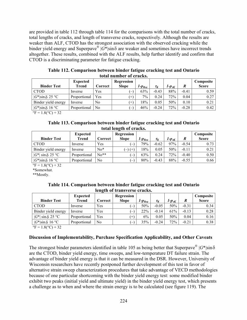
224

are provided in table 112 through table 114 for the comparisons with the total number of cracks, total lengths of cracks, and length of transverse cracks, respectively. Although the results are weaker than ALF, CTOD has the strongest association with the observed cracking while the binder yield energy and Superpave® |G*|sin are weaker and sometimes have incorrect trends altogether. These results, combined with the ALF results, help further identify and confirm that CTOD is a discriminating parameter for fatigue cracking.

Table 112. Comparison between binder fatigue cracking test and Ontario total number of cracks.

Binder Test Expected

Trend Correct Regression

Slope 1-pReg τK 1-pτΚ R Composite

Score CTOD Inverse Yes (–) 63% -0.43 88% -0.41 0.59 |G*|sin 25 °C Proportional Yes (+) 7% 0.24 72% 0.04 0.27 Binder yield energy Inverse No (+) 18% 0.05 50% 0.10 0.21 |G*|sin 16 °C Proportional No (–) 46% -0.24 72% -0.28 0.42 °F = 1.8(°C) + 32

Table 113. Comparison between binder fatigue cracking test and Ontario total length of cracks.

Binder Test Expected

Trend Correct Regression

Slope 1-pReg τK 1-pτΚ R Composite

Score CTOD Inverse Yes (–) 79% -0.62 97% -0.54 0.73 Binder yield energy Inverse No* (–) (+) 18% 0.05 50% -0.11 0.21 |G*| sin 25 °C Proportional No** (–) 63% 0.24 72% -0.40 0.50 |G*|sin 16 °C Proportional No (–) 80% -0.43 88% -0.55 0.66 °F = 1.8(°C) + 32 *Somewhat. **Mostly.

Table 114. Comparison between binder fatigue cracking test and Ontario length of transverse cracks.

Binder Test Expected

Trend Correct Regression

Slope 1-pReg τK 1-pτΚ R Composite

Score CTOD Inverse Yes (–) 50% -0.05 50% -0.31 0.34 Binder yield energy Inverse Yes (–) 22% -0.14 61% -0.13 0.28 |G*| sin 25 °C Proportional Yes (+) 6% 0.05 50% 0.04 0.16 |G*|sin 16 °C Proportional No (–) 35% -0.24 72% -0.21 0.38

°F = 1.8(°C) + 32

Discussion of Implementability, Purchase Specification Applicability, and Other Caveats

The strongest binder parameters identified in table 105 as being better that Superpave® |G*|sin are the CTOD, binder yield energy, time sweeps, and low-temperature DT failure strain. The advantage of binder yield energy is that it can be measured in the DSR. However, University of Wisconsin researchers have recently postponed further development of this test in favor of alternative strain sweep characterization procedures that take advantage of VECD methodologies because of one particular shortcoming with the binder yield energy test: some modified binder exhibit two peaks (initial yield and ultimate yield) in the binder yield energy test, which presents a challenge as to when and where the strain energy is to be calculated (see figure 119). The

δ

δ

δ

δ δ

δ δ

δ

225

VECD-based stress sweep binder test was outside the scope of this study at the time this report was written. Low-temperature failure strain was the next strongest parameter. Although low-temperature DT testing combined with BBR testing provides a more rigorous low-temperature PG grade than BBR alone, DT testing has already fallen out of favor by agencies. If this was to be reconsidered for fatigue resistance, the failure strain alone is likely vulnerable to not appropriately catching fatigue and cracking resistance because softer or lower-quality binders could exhibit higher strain tolerance. This was not the case for the legitimate, high-quality binders in this study. DT test failure strain would have to be accompanied with a strength measurement that the DT test can provide, but DENT testing at intermediate temperatures for CTOD is already a type of tension test where extension and strength are measured. Nonetheless, the largest hurdle for implementation of CTOD using DENT is the need for a new piece of test equipment if a laboratory does not already have one to measure force-ductility (AASHTO T 300).(106) Ruggedness evaluation of existing AASHTO T 300 equipment for measuring CTOD would be a necessary next step.

227

CHAPTER 8. CONCLUSIONS AND RECOMMENDATIONS

This report provides a critical evaluation of the Superpave® binder specifications |G*|/sin and |G*|sin as controlling parameters for rutting and fatigue cracking. Previously, the SHRP program explored a variety of theoretical principles and experimental techniques and ultimately selected these parameters because they are fundamental, easily measured in a DSR, and describe the dependence on temperature, frequency, and aging, all of which are relevant to factors that influence pavement performance. However, the SHRP binder validation was largely limited to unmodified asphalts. Since the implementation of Superpave®, polymer modified asphalt binder usage has become prevalent. Key research studies identified shortcomings using |G*|/sin to control rutting of polymer modified asphalts; principally, the measurement of these material properties are in the small strain, linear viscoelastic region that does not mobilize polymer structures that impart beneficial performance. Research also showed shortcomings of fatigue parameter |G*|sin , as this seemed to be valid only for thinner, unmodified asphalt pavements.

Following exploratory laboratory studies of polymer modified asphalts (NCHRP 9-10, 90-07), a full-scale APT experiment was designed.(20,22) This ALF experiment generated performance data that provided quantitative grounds to screen weaker tests and identify discriminating binder characterization parameters to potentially replace or enhance portions of the existing Superpave® PG system. Asphalt test pavements were built with a single volumetric mix design using a variety of unmodified and polymer modified binders with practically equivalent high-temperature properties and different intermediate-temperature fatigue properties.

The experiment also included pavement sections to assess the performance of crumb rubber modified asphalt. A case study for FWD layer modulus back-calculation was provided and an assessment of emerging AMPT test equipment and NCHRP MEPDG software was made.

SUMMARY AND CONCLUSIONS

Binder Performance Specification Parameters

Key findings are as follows:

• Polymer modified binders significantly improve the fatigue cracking performance compared to unmodified binders with similar high-temperature PG grades.

• There are more discriminating binder tests for fatigue cracking and rutting than standard Superpave® |G*|sin and |G*|/sin , and these tests are poised for implementation or have already become standardized, including MSCR and oscillatory-based nonrecoverable stiffness for rutting and calculated CTOD for fatigue cracking.

• Increasing polymer content in relatively softer base asphalt binders to achieve higher temperature PG grades does not necessarily provide increased fatigue cracking resistance. An important caveat of this conclusion is that it may only be applicable for the particular structural configuration of the ALF pavements in this experiment. However, the rutting performance of this mixture was generally good and comparable to the other polymer modified mixtures until large rut depths (0.47 inches (12 mm)) were reached, and then rutting increased substantially.

δ δ

δ

δ

δ δ

228

Binder Test to Discriminate Permanent Deformation and Rutting

Key findings are as follows:

• The two most discriminating, implementable parameters for rutting quantify irrecoverable deformations that occur in asphalt binder. Oscillatory-based nonrecoverable stiffness is measured in the DSR in a similar manner as the familiar |G*|/sin . MSCR has already been developed as an AASHTO provisional standard and provides an added measure of recoverable measurements and, therefore, has advantages over oscillatory-based nonrecoverable stiffness.

• The performance data in this particular experiment demonstrated that |G*|/sin still has value as a specification parameter to control rutting.

The research literature discussed in chapter 1 documents the shortcomings of the Superpave® high-temperature PG test. Namely, the test deforms the binder to small strains and has trouble capturing the performance-related effect of polymer modification. However, the rutting performance of the polymer modified and unmodified asphalt binders in this particular full-scale APT experiment do not reflect this deficiency. The binders used in this study were designed and selected to have the same high-temperature PG (see figure 15). Therefore, these binders should have exhibited the same rutting performance, which was essentially the case (see figure 28, figure 29, table 17, and table 19). There were quantifiable differences in the mean rutting, but variability in the measured performance diminished those differences. Therefore, one interpretation of this experiment’s rutting data is that |G*|/sin still has its merits as a specification parameter to control rutting.

It must be strongly emphasized that there were notable numerical and statistical challenges in making defensible comparisons between the varieties of binder candidates to identify the best tests. Ideally, such analyses use more data points with larger spread to overcome scatter. Simply using R2 was not appropriate. The Kendall’s tau measure of association method was utilized because it is better suited for small datasets and quantifies the quality of a ranking. Statistical significance (probability) was computed as well. The different quantities were combined into a single composite score. Laboratory scale performance tests were integrated to strengthen the scoring because the binder contributions are reflected in laboratory tests in addition to full-scale pavement tests, which provide the analysis with a degree of balance with the full-scale ALF performance.

Some candidate binder parameters such as LSV and ZSV were found to have a strong relation to laboratory-scale and full-scale performance. However, these parameters can be susceptible to registering improved performance from additives or modification (i.e., acid), which is not as legitimate as the beneficial improvements from polymer modification used in this study. Thus, they were not recommended.

Binder Tests to Discriminate Fatigue and Cracking

There were fewer numerical and statistical challenges in the datasets to rank weaker and stronger binder tests for fatigue cracking. The strongest analysis came from the thinner, 4-inch (100-mm)

δ

δ

δ

229

ALF lanes because two of the thicker, polymer modified mixtures in the 5.8-inch (150-mm) lanes did not exhibit any fatigue cracking. Nondestructive testing and extrapolated estimates were used to provide a reasonable measure of ranking for the whole set of 5.8-inch (150-mm) lanes.

The key finding is as follows:

• The analysis from both 4- and 5.8-inch (100- and 150-mm) lanes plus a third verification from an Ontario test site showed calculated CTOD was consistently the most discriminating. Binder yield energy was the next strongest. These results confirm tests that deform binder to very large strains discriminate fatigue resistance from polymer modification. CTOD can be considered implementable because it can be measured using a force-ductility apparatus that is available in some pavement testing laboratories.

Crumb Rubber Modified Asphalt

The key finding is as follows:

• Gap-graded crumb rubber modified asphalt mix (Arizona wet process) placed in a composite pavement structure exhibited excellent fatigue cracking resistance to bottom-up fatigue cracks. Fatigue cracks initiated and propagated up through 2 inches (50 mm) of conventional dense-graded asphalt on the bottom but did not progress through any of the 2 inches (50 mm) of gap-graded crumb rubber mix on top.

The CR-AZ mix was formulated using a PG58-22 base binder plus 17 percent crumb rubber by weight following ASTM D6114.(24) The estimated high and intermediate PG grades were 194 and 74.1 °F (90.1 and 23.4 °C), respectively using techniques developed in research based on DSR measurements on unaged binder. The CR-AZ binder could be characterized in the RTFO by tilting the oven back and in the 0.975-inch (25-mm) plate DSR using a 0.078-inch (2-mm) gap rather than a 0.039-inch (1-mm) gap. The aggregate gradation was gap-graded to accommodate the crumb rubber particles, and the binder content was 7.1 percent. The mix was produced using an onsite shearing mill at the asphalt plant. The rutting performance was similar to the dense-graded mixtures in the experiment, although the mixture has a higher binder content and somewhat lower mix dynamic modulus. The fatigue performance was the best of the 4-inch (100-mm) lanes. The ability to arrest the bottom-up fatigue cracks is attributable to the rich rubber modified binder and possibly because the stress concentration is in the lower control lift.

The CR-TB binder did not require onsite mills at the plant and was delivered and handled like conventional asphalt binder. The CR-TB mix performed well. The rutting performance was the best of all the 4-inch (100-mm) lanes because it had slightly stiffer Superpave® PG than the others, and the fatigue performance was slightly less than the SBS modified binder.

Fiber Reinforced HMA

Key findings are as follows:

• Very good fatigue cracking resistance was observed in the dense-graded mixture reinforced with polyester fibers. The fatigue cracking of this section was measurably

230

better than those of the polymer modified sections even though a less-resistant unmodified asphalt binder was used in the mix. This was the second best performer of its thickness group behind the composite, gap-graded crumb rubber asphalt pavement.

• The presence of fiber had no significant beneficial or negative impact on rutting performance.

Mixture Performance Characterization Tests

Key AMPT findings are as follows:

• AMPT flow number and SST RSCH were the two strongest laboratory indicators of ALF rutting. The AMPT flow number test is a stronger predictor and more implementable.

• Most flow number tests did not achieve tertiary flow and showed simpler two-stage curves but still adequately discriminated performance.

Key axial fatigue findings are as follows:

• An alternative test for flexural beam fatigue that used axial, DT-compression cyclic loading to capture fatigue damage modulus reduction was assessed.

• Axial fatigue with VECD can be used to generate fatigue properties at multiple conditions with a smaller experimental program than beam fatigue.

• This test was the strongest, most implementable indicator of fatigue cracking, and correcting the tests results for true strain control using VECD theory further strengthened the test’s abilities.

Other key findings are as follows:

• The importance of testing asphalt mixtures to confirm performance cannot be understated. Such testing should not rely entirely on binder tests because additives such as fibers will challenge specification tests at the binder scale, and only mixture tests are suited to accommodate pavement structural attributes and volumetric mix design characteristics.

• The fiber mix presented some challenges for the three best mixture tests for fatigue cracking; none were able to reflect higher fatigue resistance.

A variety of materials characterization tests were conducted on ALF cores, plant-produced mixtures, and laboratory-produced mixtures. Some were established tests while others were emerging tests. The following tests were utilized in this research:

• AMPT flow number: More convenient flow number tests using less confinement can produce permanent strain magnitudes and rankings similar to more confined tests so long as the deviator stress is smaller in less-confined tests. Also, predicted rutting using flow number curves from more convenient, less-confined tests can be similar to predictions

231

using confined flow number inputs because the less-confined deviator stress is accordingly smaller.

• Axial fatigue: Although the axial fatigue tests require added steps for gluing caps onto the end of the specimen, it still offers advantages over flexural beam fatigue because samples can be made in the Superpave® gyratory compactor. Axial cyclic fatigue tests in stress control rank performance in opposite manners, with stress control favoring stiffer mixtures and strain control favoring softer mixtures.

• Dynamic modulus: Dynamic modulus tests presented the best set of data to understand differences between cores versus plant-produced lab-compacted mixtures and laboratory-produced mixtures. Trends were essentially the same in all three versions where cores were measurably softer. Dynamic modulus and associated parameters that incorporate the viscous phase angle were not consistently strong indicators of rutting or fatigue cracking. However, the modulus is still absolutely necessary and an important component for mechanistic-empirical performance prediction and VECD analysis.

• TTI OT: The TTI OT captured the rank order of ALF fatigue cracking very well for a smaller group of materials but only provides an index and not an engineering property that is useful by itself for pavement design. TTI is continuing development of the test for fatigue cracking in pavement design.

• DENT: DENT mixture testing for EWF and calculated CTOD was also a fairly strong indicator of fatigue cracking, but the required number of replicates and the scatter in the analysis are drawbacks. The test also does not yield an engineering property.

• Wheel tracking: The French PRT and HWT were unable to satisfactorily capture the rank order of the full-scale ALF rutting.

• IDT strength: IDT strength alone is not a strong indicator to identify fatigue cracking resistance.

FWD

FWD testing revealed variation in the stiffness of the unbound layer within each binder’s test lane and between test lanes. Back-calculation programs EVERCALC and MODCOMP, having different optimization algorithms, were evaluated and found to provide the same trends. The average stiffness of the crushed stone base was between 11.9 and 9.6 ksi (82 and 66 MPa), slightly stiffer than the average subgrade stiffness ranging between 11.4 and 11.1 ksi (79 and 77 MPa). Known depth to bedrock was easily detected. EVERCALC moduli were chosen because the base was generally stiffer and the subgrade was generally softer. Predicted HMA tensile strain using laboratory-measured modulus and FWD back-calculated base and subgrade stiffness gave reasonable magnitudes compared to what was measured from embedded strain gauges.

The use of MDDs was key in evaluating the quality of the back-calculations. Forward predictions of the base and subgrade layer deflections using the back-calculated modulus revealed very good agreement on the top of the base layer, fair agreement in the center of the

232

base layer, and less agreement at the bottom of the base layer. This indicated that the back-calculation could have been additionally optimized. However, the focus of the experiment was the HMA layers, and the back-calculated moduli were deemed sufficient given that the critical strains and stresses for the purposes of this study were located within the asphalt layers. A seasonal monitoring program enables the depth to the seasonally-affected and unaffected subgrade layer to be estimated and identified more accurately.

Mechanistic-Empirical Pavement Performance Analysis

The key finding is as follows:

• Additional mixture-specific characterization inputs are needed above and beyond the |E*| dynamic modulus to be able to better discriminate and rank performance of modified and unmodified asphalt.

The NCHRP 1-37A and NCHRP 1-40D MEPDG models are largely calibrated using data from LTPP.(1) These do not include any significant amounts of polymer modified asphalt data, whereas the ALF experiment included several different polymer modified asphalts. Consequently, the rank order and the magnitude of predicted rutting and fatigue cracking were not accurate. In fact, the actual MEPDG software was not able to be used for the predictions because it was not developed to accommodate specialized APT conditions (i.e., controlled temperatures, heavy wheel loads). A standalone application that emulates the MEDPG had to be used.

Just as with the binder parameters previously discussed, modulus measured at small strains (binder |G*| and mixture |E*|) does not mobilize the material into regions that force the particular performance aspects to be revealed, whether permanent deformation or fatigue crack resistance. Along these lines, the NCHRP 9-30A project is pursuing this type of material characterization input and recalibration of the guide for improved rutting prediction.(90) This study illustrated an approach similar to the methodologies that will come out of NCHRP 9-30A, which use flow number permanent deformation curves to yield mixture-specific coefficients for the MEPDG model framework rather than a single national calibration for all HMA. Magnitudes of the predicted rutting were improved drastically, but the ranking was still not captured. However, the statistical similarities and variability in the measured rutting bracket the improved predictions. Additional insight gained from the flow number-based rutting prediction analysis is that the value of characterization at more than one temperature would allow a better prediction of rutting over a range of temperatures.

Two aspects of damage and fatigue cracking that the MEPDG does not provide were highlighted. Seismic PSPA tests on two ALF lanes illustrated that HMA modulus decreases by as much as 50 percent before fatigue cracks show at the surface. HMA modulus in the MEPDG is not recursively updated to reflect damage and modulus reduction. The pattern in which actual bottom-up fatigue cracking develops was not captured whereby the surface remains crack free until surface cracking is initiated and propagates.

Despite these shortcomings, the MEPDG was useful in analyzing the uniformity of ALF construction. The national calibration containing many different material characteristics and

233

structural features taken from LTPP can be assumed to adequately capture the impact variations in layer thickness, density (modulus), and base and subgrade support have on predicted rutting and fatigue. Three scenarios were evaluated: as-built, as-designed, and as-designed with fixed (average) base and subgrade stiffness. The very similar rankings revealed from the exercise indicated no significant changes in the rank order.

RECCOMENDATIONS

The following recommendations are made based on the conclusions from this research:

• Adopt CTOD for the next generation of binder specification tests for fatigue cracking resistance.

• Support continued refinement and implementation of cyclic axial fatigue protocols in AMPT equipment. This is ongoing in two FHWA-supported research activities: performance-related specifications and Western Research Institute Asphalt Research Consortium Technology Deployment activity.

• Consider application of gap-graded crumb rubber in thicker layers and pavement structures that take advantage of placing the bottom of the layer at or near a neutral axis to arrest the propagation of fatigue cracks.

• Review literature and survey agencies to evaluate performance and cost benefits of other fiber-modified HMA projects’ performance to compare and contrast with ALF performance.

A number of follow-up activities are recommended, as follows:

• Develop draft CTOD specifications in AASHTO format beginning with Ontario Method LS-299 and AASHTO T 300.(71,106)

• Fabricate molds and tabs for the DENT test and distribute to participating agencies.

• Present strengths of CTOD to AASHTO and the FWHA Asphalt ETGs to gather written comments on implementability and applicability as specification test (some presentations have been made to ETG already).

• Organize an exploratory round-robin study in preparation for ruggedness evaluation of CTOD.

• Explore the LTTP database to identify sites with different levels of fatigue cracking performance and characterize the binders for CTOD for added validation (ongoing).

• Conduct flow number tests at temperatures other than 147 °F (64 °C) to refine the flow number-based rutting performance of ALF mixture following the recommendations of NCHRP 9-30A as they are developed.

234

• Quantify the cost and benefits of fiber and crumb rubber for the particular ALF pavements structure and performance.

• Expand upon PSPA characterization of ALF lanes in future experiments.

• Ensure that absorption of cores for density is measured in future quality assurance during ALF construction and consider sampling from behind the paver rather than from within trucks.

235

APPENDIX. DENT TEST METHOD SPECIFICATION

TITLE

The title of this document is “Standard Specification for Method of Test for the Determination of Asphalt Cement’s Resistance to Ductile Failure Using Double Edge Notched Tension Test (DENT).”

SCOPE

This test method covers the determination of asphalt cement’s resistance to ductile failure using a DENT test. The test is conducted after thermal conditioning to determine the EWF, the plastic work of fracture, and an approximate CTOD at a specified temperature and rate of loading. This method is provided as a provisional test method. The test is a working document; continuous refinement to the test method may be expected.

REFERENCED DOCUMENTS

The following documents are referenced in this specification:

• AASHTO R 28, Accelerated Aging of Asphalt Cement Using a Pressurized Aging Vessel (PAV).

• AASHTO T 240, Effect of Heat and Air on a Moving Film of Asphalt (Rolling Thin-Film Oven Test).

• AASHTO T 300, Force-Ductility Test of Bituminous Materials.

• AASHTO T 301, Elastic Recovery Test of Asphalt Materials by Means of a Ductilometer.

• AASHTO T 315, Determining the Rheological Properties of Asphalt Binder Using a Dynamic Shear Rheometer (DSR).

• ASTM D8, “Standard Definitions of Terms Relating to Materials for Roads and Pavements.”

• ASTM D113, “Standard Test Method for Ductility of Bituminous Materials.”

• MTO LS-299, Method of Test for Determining Asphalt Cement’s Resistance to Ductile Failure Using Double-Edge-Notched Tension Tests (Ministry of Transportation, Ontario).

TERMINOLOGY

The following terminology is used in this specification:

• Wt = Total work of fracture, area under the load versus load-line displacement curve, units J.

236

• wt = Specific total work of fracture (Wt / Bℓ), units kJ/m2.

• we = Specific EWF, the energy required to fracture or break the sample without plastic deformation away from the fracture zone, units kJ/m2.

• wp = Specific plastic work of fracture, the non-essential work dissipated during the deformation of a volume of asphalt around the fracture zone, units MJ/m3.

• β = Geometric constant describing the shape of the plastic zone.

• δt = CTOD, units mm.

• P = Load, units N.

• D = Displacement in test, units m.

• B = Sample thickness, units m.

• ℓ = Ligament length, the material between the notches, units m.

• σn = Net section stress of sample, units N/m2.

APPARATUS

The following equipment is used in this specification:

• Mold: Consists of two end pieces and a pair of matching DENT inserts fitted together as shown in AASHTO T301.

• End pieces: Six end pieces from the elastic recovery specimen mold according to AASHTO T 301.

• DENT inserts: Six inserts made from type 360 brass, built to dimensions shown in figure 186. These inserts come in pairs, and each pair is manufactured to have a space between the matching pair of notches equal to the three different ligament lengths of 0.59, 0.39, and 0.2 inches (15, 10, and 5 mm) when fitted with the end pieces.

237

1 mm = 0.039 inches

Figure 186. Illustration. DENT inserts.

• Base plates: The base plates shall be made of non-absorbent material of sufficient thickness to prevent deformation and of a sufficient size to hold from one to three molds, but still able to fit in the temperature-controlled bath for conditioning. The plate shall be uniformly flat to ensure that the bottom surfaces of each mold will touch it throughout.

• Testing apparatus: A constant rate of displacement device capable of maintaining displacement at rates of 4 ±0.01 inches/min (100 ±2.5 mm/min). The maximum stroke for the instrument shall be 39.4 inches (1,000 mm) or greater. The apparatus should have a set of loading pins that ensure precise alignment of the sample during the test. The apparatus shall be able to determine displacement to an accuracy of 0.002 inches (±0.05 mm). (Note: DENT testing apparatus is commonly force-ductility apparatus installed in a ductilometer.)

• Load sensor: The sensitivity of the load sensor and recording electronics shall allow the load, P, to be measured every 0.3 s during the test with an accuracy of at least ±1 percent. The load sensor shall be capable of measuring a nominal maximum force of up to 29.9 lbf (133 N).

• Temperature-controlled bath for testing: The bath shall be large enough to contain the testing apparatus and samples in their molds prior to testing under a minimum of 1 inch (25 mm) of water. The equipment shall be capable of maintaining the water at the testing temperature to an accuracy of at least ±0.9 °F (±0.5 °C).

• Temperature-controlled bath for conditioning: The bath shall be capable of maintaining a minimum of 1 inch (25 mm) of water over the sample at the conditioning temperature requirements to within ±0.9 °F (±0.5 °C). Typically, the temperature-controlled bath for testing is utilized.

• Glass stir: Stick capable of stirring the hot asphalt cement vigorously.

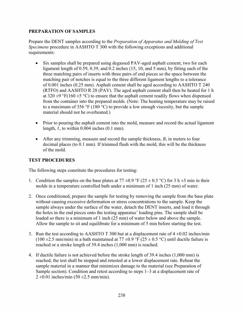
238

PREPARATION OF SAMPLES

Prepare the DENT samples according to the Preparation of Apparatus and Molding of Test Specimens procedure in AASHTO T 300 with the following exceptions and additional requirements:

• Six samples shall be prepared using degassed PAV-aged asphalt cement, two for each ligament length of 0.59, 0.39, and 0.2 inches (15, 10, and 5 mm), by fitting each of the three matching pairs of inserts with three pairs of end pieces so the space between the matching pair of notches is equal to the three different ligament lengths to a tolerance of 0.001 inches (0.25 mm). Asphalt cement shall be aged according to AASHTO T 240 (RTFO) and AASHTO R 28 (PAV). The aged asphalt cement shall then be heated for 1 h at 320 ±9 °F(160 ±5 °C) to ensure that the asphalt cement readily flows when dispensed from the container into the prepared molds. (Note: The heating temperature may be raised to a maximum of 356 °F (180 °C) to provide a low enough viscosity, but the sample material should not be overheated.)

• Prior to pouring the asphalt cement into the mold, measure and record the actual ligament length, ℓ, to within 0.004 inches (0.1 mm).

• After any trimming, measure and record the sample thickness, B, in meters to four decimal places (to 0.1 mm). If trimmed flush with the mold, this will be the thickness of the mold.

TEST PROCEDURES

The following steps constitute the procedures for testing:

1. Condition the samples on the base plates at 77 ±0.9 °F (25 ± 0.5 °C) for 3 h ±5 min in their molds in a temperature controlled bath under a minimum of 1 inch (25 mm) of water.

2. Once conditioned, prepare the sample for testing by removing the sample from the base plate without causing excessive deformation or stress concentrations to the sample. Keep the sample always under the surface of the water, detach the DENT inserts, and load it through the holes in the end pieces onto the testing apparatus’ loading pins. The sample shall be loaded so there is a minimum of 1 inch (25 mm) of water below and above the sample. Allow the sample to sit and equilibrate for a minimum of 5 min before starting the test.

3. Run the test according to AASHTO T 300 but at a displacement rate of 4 ±0.02 inches/min (100 ±2.5 mm/min) in a bath maintained at 77 ±0.9 °F (25 ± 0.5 °C) until ductile failure is reached or a stroke length of 39.4 inches (1,000 mm) is reached.

4. If ductile failure is not achieved before the stroke length of 39.4 inches (1,000 mm) is reached, the test shall be stopped and retested at a lower displacement rate. Reheat the sample material in a manner that minimizes damage to the material (see Preparation of Sample section). Condition and retest according to steps 1–3 at a displacement rate of 2 ±0.01 inches/min (50 ±2.5 mm/min).

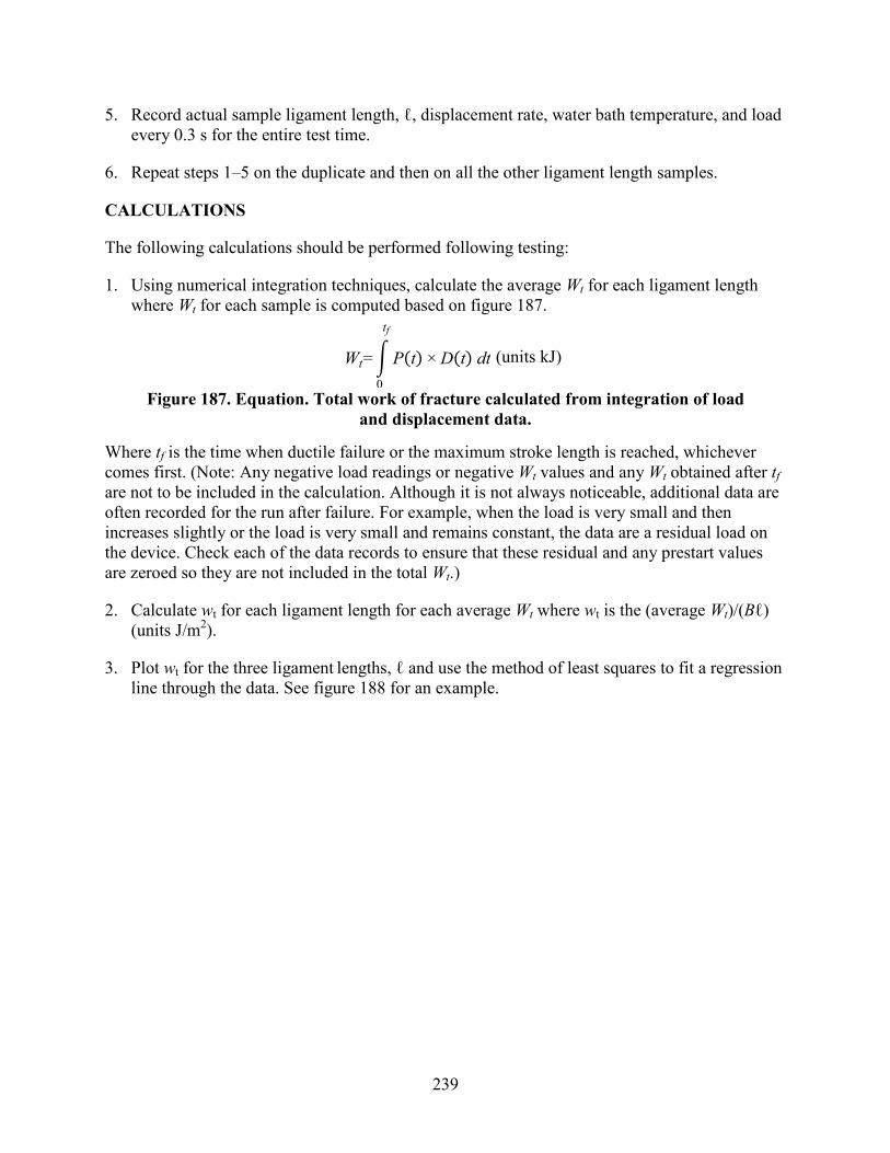
239

5. Record actual sample ligament length, ℓ, displacement rate, water bath temperature, and load every 0.3 s for the entire test time.

6. Repeat steps 1–5 on the duplicate and then on all the other ligament length samples.

CALCULATIONS

The following calculations should be performed following testing:

1. Using numerical integration techniques, calculate the average Wt for each ligament length where Wt for each sample is computed based on figure 187.

(units kJ)

Figure 187. Equation. Total work of fracture calculated from integration of load and displacement data.

Where tf is the time when ductile failure or the maximum stroke length is reached, whichever comes first. (Note: Any negative load readings or negative Wt values and any Wt obtained after tf are not to be included in the calculation. Although it is not always noticeable, additional data are often recorded for the run after failure. For example, when the load is very small and then increases slightly or the load is very small and remains constant, the data are a residual load on the device. Check each of the data records to ensure that these residual and any prestart values are zeroed so they are not included in the total Wt.)

2. Calculate wt for each ligament length for each average Wt where wt is the (average Wt)/(Bℓ) (units J/m2).

3. Plot wt for the three ligament lengths, ℓ and use the method of least squares to fit a regression line through the data. See figure 188 for an example.

Wt=�P(t) × D(t) dt

tf

0

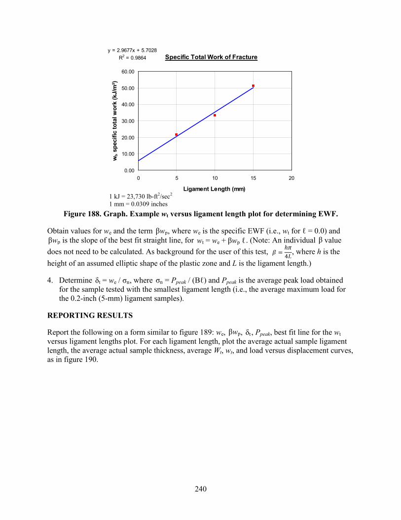
240

1 kJ = 23,730 lb-ft2/sec2

1 mm = 0.0309 inches Figure 188. Graph. Example wt versus ligament length plot for determining EWF.

Obtain values for we and the term , where we is the specific EWF (i.e., wt for ℓ = 0.0) and is the slope of the best fit straight line, for . (Note: An individual value

does not need to be calculated. As background for the user of this test, , where h is the height of an assumed elliptic shape of the plastic zone and L is the ligament length.)

4. Determine , where = Ppeak / (Bℓ) and Ppeak is the average peak load obtained for the sample tested with the smallest ligament length (i.e., the average maximum load for the 0.2-inch (5-mm) ligament samples).

REPORTING RESULTS

Report the following on a form similar to figure 189: we, , , Ppeak, best fit line for the wt versus ligament lengths plot. For each ligament length, plot the average actual sample ligament length, the average actual sample thickness, average Wt, wt, and load versus displacement curves, as in figure 190.

Specific Total Work of Fracturey = 2.9677x + 5.7028

R2 = 0.9864

0.00

10.00

20.00

30.00

40.00

50.00

60.00

0 5 10 15 20

Ligament Length (mm)

wt,

spec

ific

tota

l wor

k (k

J/m

²)

βwp βwp wt = we + βwp ℓ β

𝛽𝛽 =ℎ𝜋𝜋4𝐿𝐿

δt = we / σn σn

βwp δt

241

Figure 189. Chart. Example reporting sheet.

242

1 N = 0.225 lbf 1 mm = 0.0309 inches

Figure 190. Graph. Typical load-displacement curves for EWF test.

Load Versus Displacement Curves

0

20

40

60

80

100

120

140

0 25 50 75 100 125 150 175 200

Displacement (mm)

Load

(N)

5mm - Run 15mm - Run 210mm - Run 110mm - Run 215mm - Run 115mm - Run 2

243

ACKNOWLEDGEMENTS

There are many organizations and people to thank for support of this research. Most notably, the financial support through the TPF and State Planning and Research programs by the following State transportation departments: Connecticut, Florida, Iowa, Illinois, Kansas, Maryland, Michigan, Minnesota, Mississippi, Montana, North Carolina, Nebraska, Nevada, New Jersey, New York, Oregon, Pennsylvania, and Texas.

Significant credit is also given to the following private industry organizations that provided in-kind contributions: NuStar (formerly Citgo), Dow, DuPont, Road Science LLC (formerly Koch), Paramount, Butaphalt (formerly TexPar), Trifinery GCA, Trumbull, Owens Corning, Wright Asphalt, Martin Color Fi, Bit Mat, Mathy Construction/MTE Services, the National Asphalt Pavement Association, FNF Construction, Consulpav, Rubber Pavements Association, International Surfacing Systems, and Recovery Technologies Group.

A great deal of recognition must be made to FWHA staff John D’Angelo (retired), Tom Harman, Kevin Stuart (retired), and Jack Youtcheff for identifying, developing, and coordinating the experiment. In addition, the members of the FWHA Asphalt ETGs and their associated State transportation department and private industry friends and members are acknowledged for their input on the experiment’s development.

ALF construction and many FWD tests could not have completed without the efforts and services of FHWA Eastern Federal Lands.

FHWA MAMTL provided very valuable onsite testing during construction for quality assurance in participation with the TFHRC Bituminous Mixtures Laboratory.

The final report could not have been assembled without contributions from research support staff and associates in the ALF operations. Binder Rheology Laboratory and Bituminous Mixtures staff were Dennis Lim, Mario Tinio, Susan Needham, Scott Parobeck, Frank Davis, and Senthil Thyagarajan.

245

REFERENCES

1. National Cooperative Highway Research Program Project 1-37(A). (2004). Mechanistic-Empirical Design Guide of New and Rehabilitated Pavement Structures, Washington, DC. Obtained from: http://onlinepubs.trb.org/onlinepubs/archive/mepdg/home.htm.

2. AASHTO M 320. (2009). Standard Specification for Performance-Graded Asphalt Binder, American Association of State Highway and Transportation Officials, Washington, DC.

3. AASHTO T 313. (2012). Standard Method of Test for Determining the Flexural Creep Stiffness of Asphalt Binder Using the Bending Beam Rheometer (BBR), American Association of State Highway and Transportation Officials, Washington, DC.

4. AASHTO T 314. (2012). Standard Method of Test for Determining the Fracture Properties of Asphalt Binder in Direct Tension (DT), American Association of State Highway and Transportation Officials, Washington, DC.

5. AASHTO T 315. (2012). Standard Method of Test for Determining the Rheological Properties of Asphalt Binder Using a Dynamic Shear Rheometer (DSR), American Association of State Highway and Transportation Officials, Washington, DC.

6. Petersen, J.C., Robertson, R., Brenthaver, J., Harnsberger, P.M., Duval, J., Kim, S., Anderson, D., Christensen, D., and Bahia, H. (1994). Binder Characterization and Evaluation, Volume 1, Report No. SHRP A-367, Strategic Highway Research Program, National Research Council, Washington, DC.

7. Kennedy, T.W, Cominsky, R.J., Harrigan, E., and Leahy, R. (1990). The SHRP Asphalt Research Program: 1990 Strategic Planning Document, Report No. SHRP-A/UWP-90-007, Strategic Highway Research Program, National Research Council, Washington, DC.

8. Anderson, D., Christensen, D., Bahia, H., Dongre, R., Sharma, M., Antle, C., and Button, J. (1994). Binder Characterization and Evaluation, Volume 3: Physical Characterization, Report No. SHRP A-369, Strategic Highway Research Program, National Research Council, Washington, DC.

9. Hveem, F., Zube, E., and Skog, J. (1960). “Progress Report on the Zaca-Wigmore Experimental Asphalt Test Project,” Symposium on Road and Paving Materials, 1959, ASTM STP 277, American Society for Testing and Materials, Baltimore, MD.

10. Skog, J.B. (1981). “Effect of Changes in Asphalt Properties on Pavement Performance: Zaca-Wigmore Test Road,” Asphalt Paving Technology, Proceedings of the Association of Asphalt Paving Technologists Technical Session, Vol. 50.

11. Deacon, J.A., Tayebali, A., Coplantz, J., Finn, F., and Monismith, C. (1994). Fatigue Response of Asphalt-Aggregate Mixes; Part III: Mix Design and Analysis, Report No. SHRP A-404, Strategic Highway Research Program, National Research Council, Washington, DC.

246

12. Asphalt Research Program, University of California, Berkley. (1994). Permanent Deformation Response of Asphalt Aggregate Mixes, Report No. SHRP A-415, Strategic Highway Research Program, National Research Council, Washington, DC.

13. Strategic Highway Research Program. (1994). Stage 1 Validation of the Relationship Between Asphalt Properties and Asphalt-Aggregate Mix Performance, Report No. SHRP A-398, National Research Council, Washington, DC.

14. Leahy, R.B., Monismith, C.L., and Lundy, J.L. (1995). “Performance-Based Properties of Asphalt Concrete Mixtures,” Engineering Properties of Asphalt Mixtures and the Relationship to their Performance, ASTM STP 1265, G. Huber and D. Decker (Eds.), ASTM International, Philadelphia, PA.

15. Lytton, R., Uzan, J., Fernando, E., Roque, R., Hiltunen, D., and Stoffels, S., (1993). Development and Validation of Performance Prediction Models and Specifications for Asphalt Binders and Paving Mixes, Report No. SHRP A-357, Strategic Highway Research Program, National Research Council, Washington, DC.

16. Stuart, K.D., Mogawer, W.S., and Romero, P. (2001). Validation of the Superpave Asphalt Binder Fatigue Cracking Parameter Using the FHWA’s Accelerated Loading, Report No. FHWA-RD-01-093, Federal Highway Administration, McLean, VA.

17. Stuart, K.D. and Mogawer, W.S. (1997). “Validation of Asphalt Binder and Mixture Tests that Predict Rutting Susceptibility Using the Federal Highway Administration’s Accelerated Loading Facility,” Journal of the Association of Asphalt Paving Technologists, Vol. 66.

18. Stuart, K.D., Mogawer, W.S., and Romero, P. (1999). Validation of Asphalt Binder and Mixture Tests That Measure Rutting Susceptibility Using the Accelerated Loading Facility, Report No. FHWA-RD-99-204, Federal Highway Administration, McLean, VA.

19. Kavanaugh, L. (2004). “A 9-Year Evaluation of Field Cracking and Rutting Performance of SPS-9 Superpave Experiment,” Transportation Research Record 1896, Transportation Research Board, National Academy of Science, Washington, DC.

20. Bahia, H., Hanson, D., Zeng, M., Zhai, H., Khatri, M., and Anderson, R. (2001). Characterization of Modified Asphalt Binders in Superpave Mix Design, NCHRP Report 459, National Cooperative Highway Research Program, National Academy of Science, Washington, DC.

21. Deacon, J., Harvey, J., Tayebali, A., and Monismith, C. (1997). “Influence of Binder Loss Modulus on the Fatigue Performance of Asphalt Concrete Pavements,” Journal of the Association of Asphalt Paving Technologists, Vol. 66.

22. Stuart, K.D., Youtcheff, J.S., and Mogawer, W.S. (2001). Understanding the Performance of Modified Asphalt Binders in Mixtures: Evaluation of Moisture Sensitivity, Report No. FHWA-RD-02-029, Federal Highway Administration, McLean, VA.

247

23. Arizona Test Method 714. (2006). Sampling and Sieving of Crumb Rubber, Arizona Department of Transportation, Phoenix, AZ.

24. ASTM D6114/D6114M. (2009). Standard Specification for Asphalt-Rubber Binder, ASTM International, West Conshohocken, PA.

25. ASTM D5329. (2009). Standard Test Methods for Sealants and Fillers, Hot-Applied, for Joints and Cracks in Asphaltic and Portland Cement Concrete Pavements, ASTM International, West Conshohocken, PA.

26. ASTM D36/D36M. (2012). Standard Test Method for Softening Point of Bitumen (Ring-and-Ball Apparatus), ASTM International, West Conshohocken, PA.

27. ASTM D5. (2006). Standard Test Method for Penetration of Bituminous Materials, ASTM International, West Conshohocken, PA.

28. Shenoy, A. (2001). “High Temperature Performance Grade Specification of Paving Asphalt from the Material’s Volumetric-Flow Rate,” Materials and Structures, Vol. 24, No. 244.

29. Shenoy, A. (2002). “A Method to Estimate the Rheological Properties of Aged Asphalt Binders Without Actually Aging Them,” Road Materials and Pavement Design, Vol. 64.

30. Arizona Department of Transportation. (2008). “Section 413, Asphaltic Concrete (Asphalt-Rubber),” Standard Specifications for Road and Bridge Construction, Phoenix, AZ.

31. Bonaquist, R. (1992). An Assessment of the Increased Damage Potential of Wide Base Single Tires, Proceedings, 7th International Conference on Asphalt Pavements, Vol. 3.

32. Sherwood, J. (2005). Ultra-Thin Whitetopping (UTW) Project, Accelerated Pavement Testing of Ultra-Thin Whitetopping Concrete Overlays, Federal Highway Administration, McLean, VA. Obtained from: http://www.fhwa.dot.gov/pavement/utwweb/. Site last accessed November 7, 2011.

33. University of Illinois at Urbana-Champaign, Construction Technologies Laboratories, and The Asphalt Institute. (1990). Calibrated Mechanistic Structural Analysis Procedure for Pavements: Volume II, Appendices, NCHRP Project 1-26, Final Report. Transportation Research Board, National Research Council, Washington, DC.

34. Anderson, D.A., Kilareski, W.P., and Siddiqui, Z. (1988). Pavement Testing Facility: Design and Construction, Report No. FHWA-RD-88-059, Federal Highway Administration, Washington, DC.

35. AASHTO T 99. (2010). Standard Method of Test for Moisture-Density Relations of Soils Using a 2.5-kg (5.5-lb) Rammer and a 305-mm (12-in.) Drop, American Association of State Highway and Transportation Officials, Washington, DC.

248

36. AASHTO T 180. (2010). Standard Method of Test for Moisture-Density Relations of Soils Using a 4.54-kg (10-lb) Rammer and a 457-mm (18-in.) Drop, American Association of State Highway and Transportation Officials, Washington, DC.

37. AASHTO T 168. (2003). Standard Method of Test for Sampling Bituminous Paving Mixtures, American Association of State Highway and Transportation Officials, Washington, DC.

38. AASHTO T 248. (2011). Standard Method of Test for Reducing Samples of Aggregate to Testing Size, American Association of State Highway and Transportation Officials, Washington, DC.

39. AASHTO T 30. (2010). Standard Method of Test for Mechanical Analysis of Extracted Aggregate, American Association of State Highway and Transportation Officials, Washington, DC.

40. AASHTO T 308. (2010). Standard Method of Test for Determining the Asphalt Binder Content of Hot Mix Asphalt (HMA) by the Ignition Method, American Association of State Highway and Transportation Officials, Washington, DC.

41. AASHTO T 287. (2006). Standard Method of Test for Asphalt Binder Content of Asphalt Mixtures by the Nuclear Method, American Association of State Highway and Transportation Officials, Washington, DC.

42. AASHTO T 209. (2012). Standard Method of Test for Theoretical Maximum Specific Gravity (Gmm) and Density of Hot Mix Asphalt (HMA), American Association of State Highway and Transportation Officials, Washington, DC.

43. AASHTO PP28. (2001). Standard Practice for Superpave Volumetric Design for Hot Mix Asphalt (HMA), American Association of State Highway and Transportation Officials, Washington, DC.

44. ASTM D2950/D2950M. (2011). Standard Test Method for Density of Bituminous Concrete in Place by Nuclear Methods, ASTM International, West Conshohocken, PA.

45. AASHTO T 166. (2012). Standard Method of Test for Bulk Specific Gravity (Gmb) of Compacted Hot Mix Asphalt (HMA) Using Saturated Surface-Dry Specimens, American Association of State Highway and Transportation Officials, Washington, DC.

46. ASTM D3203/D3203M. (2011). Standard Test Method for Percent Air Voids in Compacted Dense and Open Bituminous Paving Mixtures, ASTM International, West Conshohocken, PA.

47. FLH T 501-96. (1996). “Determining the Thickness of Compacted Asphalt Concrete Paving Mixture Specimens,” Federal Lands Highway Field Materials Manual, Office of Federal Lands Highway, Federal Highway Administration, Washington, DC.

249

48. Arnold, T.S., Rozario-Ranasinghe, M., and Youtcheff, J. (2006). “Determination of Lime in Hot-Mix Asphalt,” Transportation Research Record 1962, Transportation Research Board, National Academy of Science, Washington, DC.

49. Qi, X., Gibson, N., and Youtcheff, J. (2008). Fatigue Cracking Characteristics of Accelerated Testing Pavements with Modified Binders, Proceedings of the Sixth RILEM International Conference on Cracking in Pavements, June 16–18, Chicago, IL.

50. Youtcheff, J., Stuart, K., Al-Khateeb, G., and Shenoy, A. (2004). Understanding the Performance of Polymer Modified Binders, Proceedings of the Eurasphalt and Eurobitme Congress, May 12–14, Vienna, Austria.

51. AASHTO T 331. (2010). Standard Method of Test for Bulk Specific Gravity and Density of Compacted Hot Mix Asphalt (HMA) Using Automatic Vacuum Sealing Method, American Association of State Highway and Transportation Officials, Washington, DC.

52. Kendall, M. and Gibbons, J. (1996). Rank Correlation Methods, Fifth Edition, Oxford University Press, Oxford, England.

53. Washington, S., Leonard, J., Manning, D.G., Roberts, C., Williams, B., and Bacchus, A.R. (2001). NCHRP 20-45—Statistics for Transportation Researchers, Scientific Approaches to Transportation Research, National Cooperative Highway Research Program. Obtained from: http://onlinepubs.trb.org/onlinepubs/nchrp/cd-22/readme.html. Site last accessed November 7, 2011.

54. Bari, J. (2006). Development of a New Revised Version of the Witczak E* Predictive Models for Hot Mix Asphalt Mixtures, Ph.D. dissertation, Arizona State University, Phoenix, AZ.

55. Washington State Department of Transportation. (2005). Everseries User’s Guide, Pavement Analysis Computer Software and Case Studies. Obtained from: http://www. wsdot.wa.gov/Business/MaterialsLab/Pavements/PavementDesign.htm#FWD. Site last accessed November 7, 2011.

56. AASHTO TP 79-09. (2009). Standard Method of Test for Determining the Dynamic Modulus and Flow Number for Hot Mix Asphalt (HMA) Using the Asphalt Mixture Performance Tester (AMPT), American Association of State Highway and Transportation Officials, Washington, DC.

57. Thyagarajan, S., Sivaneswaran, N., Muhunthan, B., and Petros, K. (2009). “An Evaluation of the Effects of Nonlinear Load-Strain Behavior on MEPDG Analysis of Flexible Pavements,” Journal of the Association of Asphalt Paving Technologists, Vol. 78.

58. Peterson, R.L., Mahboub, K.C., Anderson, R.M., Masad, E., and Tashman, L. (2004). “Comparing Superpave Gyratory Compactor Data to Field Cores,” Journal of Materials in Civil Engineering, January/February.

250

59. Hunter, A.E., Airey, G.D., and Collop, A.C. (2004). “Aggregate Orientation and Segregation in Laboratory-Compacted Asphalt Samples,” Transportation Research Record 1891, Transportation Research Board, National Research Council, Washington, DC.

60. Wang, W. and Hoeg, K. (2009). “Method of Compaction has Significant Effects on Stress-Strain Behavior of Hydraulic Asphalt Concrete,” ASTM Journal of Testing and Evaluation, Volume 37, No. 3.

61. Linden R.N., Mahoney, J.P., and Jackson, N.C. (1989). “Effect of Compaction on Asphalt Concrete Performance,” Transportation Research Record 1217, Transportation Research Board, National Research Council, Washington, DC.

62. Abd El Halim, A.O., and Haas, R. (1994). “Effect of Field Compaction Method on Fatigue Life of Asphalt Pavements,” Transportation Research Record 1469, Transportation Research Board, National Research Council, Washington, DC.

63. Christensen, D., Pellinen, T., and Bonaquist, R. (2003). “Hirsch Model for Estimating the Modulus of Asphalt Concrete,” Journal of the Association of Asphalt Paving Technologists, Vol. 72.

64. Witczak, M.W., Kaloush, K., Pellinen, T., El-Basyouny, M., and Von Quintus, H. (2002). NCHRP Report 465: Simple Performance Test for Superpave Mix Design, Transportation Research Board, National Research Council, Washington, DC.

65. Martono, W. and Bahia, H. (2008). Developing a Surrogate Test for Fatigue of Asphalt Binders, Transportation Research Board 87th Annual Meeting Compendium of Papers, Washington, DC.

66. Shenoy, A. (2002). “Fatigue Testing and Evaluation of Asphalt Binders Using the Dynamic Shear Rheometer,” ASTM Journal of Testing and Evaluation 30(4), ASTM International, Philadelphia, PA.

67. Andriescu, A., Hesp, S.A.M., and Youtcheff, J.S. (2004). “Essential and Plastic Works of Ductile Fracture in Asphalt Binders,” Transportation Research Record 1875, Transportation Research Board, National Research Council, Washington, DC.

68. Broberg, K.B. (1975). “On Stable Crack Growth,” Journal of the Mechanics and Physics of Solids, Vol. 23, Issue 3.

69. Cotterell, B. and Reddel, J.K. (1977). “The Essential Work of Plane Stress Ductile Fracture.” International Journal of Fracture, Vol. 13, Issue 3.

70. Mai, Y.W. and Cotterell, B. (1980). “Effects of Pre-Strain on Plane Stress Ductile Fracture in α-brass,” Journal of Materials Science, Vol. 15, No. 9.

71. MOT LS-299. (2009). “Method of Test for Determining Asphalt Cement’s Resistance to Fatigue Fracture Using Double Edge Notched Tension Test (DENT),” MTO Laboratory Testing Manual, Ontario Ministry of Transportation, Downsview, ON.

251

72. Johnson, C., Wen, H., and Bahia, H. (2009). “Practical Application of Viscoelastic Continuum Damage Theory to Asphalt Binder Fatigue Characterization,” Asphalt Paving Technology, Vol. 78.

73. AASHTO TP 70. (2012). Standard Method of Test for Multiple Stress Creep Recovery (MSCR) Test of Asphalt Binder Using a Dynamic Shear Rheometer (DSR), American Association of State Highway and Transportation Officials, Washington, DC.

74. Dongré, R., D’Angelo, J., Baumgardner, G., and Reinke, G. (2003). New Developments in Refinement of the Superpave High Temperature Specification Parameter, 40th Annual Meeting of the Petersen Asphalt Research Conference, Laramie, WY.

75. Dongré, R.N. and D’Angelo, J.A. (2004). New Criterion for Superpave High-Temperature Binder Specification, 83d Annual Meeting of the Transportation Research Board, Washington, DC.

76. ASTM D5976. (2000). Standard Specification for Type I Polymer Modified Asphalt Cement for Use in Pavement Construction, ASTM International, West Conshohocken, PA.

77. AASHTO T 51. (2009). Standard Method of Test for Ductility of Asphalt Materials, American Association of State Highway and Transportation Officials, Washington, DC.

78. Shenoy, A. (2001). “Refinement of the Superpave Specification Parameter for Performance Grading of Asphalt,” Journal of Transportation Engineering, Vol. 127, Issue 5.

79. Shenoy, A. (2004). “High Temperature Performance Grading of Asphalts Through a Specification Criterion that Could Capture Field Performance,” Journal of Transportation Engineering, Vol. 130, Issue 1.

80. Shenoy, A (2004). “A Comprehensive Treatise of the High Temperature Specification Parameter,” Applied Rheology, Vol. 14, Issue 6.

81. Shenoy, A. (2008). “Nonrecovered Compliance from Dynamic Oscillatory Test Vis-a-Vis Nonrecovered Compliance from Multiple Stress Creep Recovery Test in the Dynamic Shear Rheometer,” International Journal of Pavement Engineering, Vol. 9, Issue 5.

82. Rowe, G.M., D’Angelo, J., and Sharrock, M.J. (2002). Use of the Zero Shear Viscosity as a Parameter for the High Temperature Binder Specification Parameter, 3d International Symposium on Binder Rheology and Pavement Performance, San Antonio, TX.

83. D’Angelo, J. and Dongré, R. (2004). Multi-Stress Creep Recovery: A New Approach to the Refinement of High Temperature Binder Specification, 41st Annual Meeting of the Petersen Asphalt Research Conference, Cheyenne, WY.

84. Dongré, R.N. and D’Angelo, J.A. (2006). Development of a High Temperature Performance-Based Specification in the United States, 10th International Conference on Asphalt Pavements, Quebec, Canada.

252

85. Shenoy, A. (2001). “High Temperature Performance Grade Specification of Asphalt Binder from the Material’s Volumetric-Flow Rate,” Materials and Structures, Vol. 34.

86. Shenoy, A. (2000). “Material’s Volumetric-Flow Rate (MVR) as a Unification Parameter in Asphalt Rheology and Quality Control/Quality Assurance Tool for High Temperature Performance Grading,” Applied Rheology, Vol. 10, Issue 6.

87. ASTM D1238. (2010). Standard Test Method for Melt Flow Rates of Thermoplastics by Extrusion Plastometer, ASTM International, West Conshohocken, PA.

88. AASHTO T 324. (2011). Standard Method of Test for Hamburg Wheel-Track Testing of Compacted Hot Mix Asphalt (HMA), American Association of State Highway and Transportation Officials, Washington, DC.

89. AASHTO TP 7-94. (1994). Test Method for Determining the Permanent Deformation and Fatigue Cracking Characteristics of Hot Mix Asphalt (HMA) Using the Simple Shear Test (SST) Device, American Association of State Highway and Transportation Officials, Washington, DC.

90. National Cooperative Highway Research Program NCHRP 09-30A. (Active). Calibration of Rutting Models for HMA Structural and Mix Design, Transportation Research Board, Washington, DC. Obtained from: http://apps.trb.org/cmsfeed/TRBNetProjectDisplay. asp?ProjectID=965. Site last accessed November 7, 2011.

91. Gibson N., Kutay M.E., Keramat D., and Youtcheff J. (2009). “Multiaxial Strain Response of Asphalt Concrete Measure During Flow Number Simple Performance Test,” Journal of the Association of Asphalt Paving Technologists, Vol. 78.

92. Kim, R., Guddati, M.N., Underwood, B.S., Yun, T.Y., Subramanian, V., and Savadatti, S. (2009). Development of a Multiaxial VEPCD-FEP++: Final Report, Report No. FHWA-HRT-08-073, Federal Highway Administration, Washington, DC.

93. Zhou, F., Hu, S., Chen, D., and Scullion, T. (2007). “Overlay Tester—Simple Performance Test for Fatigue Cracking,” Transportation Research Record 2001, Transportation Research Board, National Research Council, Washington, DC.

94. AASHTO T 322. (2007). Standard Method of Test for Determining the Creep Compliance and Strength of Hot Mix Asphalt (HMA) Using the Indirect Tensile Test Device, American Association of State Highway and Transportation Officials, Washington, DC.

95. AASHTO TP 8-94. (1994). Standard Test Method for Determination of the Fatigue Life of Compacted HMA Subjected to Repeated Flexural Bending, American Association of State Highway and Transportation Officials, Washington, DC.

96. Witczak, M.W. (2005). NCHRP Report 547: Simple Performance Tests: Summary of Recommended Methods and Database, Transportation Research Board, National Research Council, Washington, DC.

253

97. Lee, H.J. and Kim, Y.R. (1998). “Viscoelastic Constitutive Model for Asphalt Concrete Under Cyclic Loading,” Journal of Engineering Mechanics, Vol. 124, No. 1, American Society of Civil Engineers, Reston, VA.

98. Lee, H.J. and Kim, Y.R. (1998). “Viscoelastic Continuum Damage Model for Asphalt Concrete with Healing,” Journal of Engineering Mechanics, Vol. 124, No. 11, American Society of Civil Engineers, Reston, VA.

99. Christensen, D. and Bonaquist, R. (2005). “Practical Application of Continuum Damage Theory to Fatigue Phenomena in Asphalt Concrete Mixtures,” Journal of the Association of Asphalt Paving Technologists, Vol. 74.

100. Kutay, M.E., Gibson, N.H., and Youtcheff, J. (2008). “Conventional and Viscoelastic Continuum Damage (VECD) Based Fatigue Analysis of Polymer Modified Asphalt Pavements,” Journal of the Association of Asphalt Paving Technologists, Vol. 77.

101. Christensen, D. and Bonaquist, R. (2008). “Analysis of HMA Fatigue Data Using the Concepts of Reduced Loading Cycles and Endurance Limit,” Journal of the Association of Asphalt Paving Technologists, Vol. 78.

102. Kutay, M.E., Gibson, N.H., Dongre, R., and Youtcheff, J. (2009). “Use of Small Samples to Predict Fatigue Lives of Field Cores-Newly Developed Formulation Based on Viscoelastic Continuum Damage Theory,” Transportation Research Record 2127, Transportation Research Board, National Research Council, Washington, DC.

103. Hou, T., Underwood, B.S., and Kim, Y.R. (2010). “Fatigue Performance Prediction of North Carolina Mixtures Using the Simplified Viscoelastic Continuum Damage Model,” Journal of the Association of Asphalt Paving Technologists, Vol. 80.

104. Andriescu, A. (2006). Essential Work of Fracture Approach to Fatigue Grading of Asphalt Binders. Doctoral dissertation, Queen’s University, Kingston, Ontario.

105. Huber, G. (2009). Evaluation of Low Temperature Cracking of Hot Mix Asphalt Pavements in Ontario, A report prepared for The Ministry of Transportation of Ontario and Ontario Hot Mix Producers Association, Ontario, Canada.

106. AASHTO T 300. (2011). Standard Method of Test for Force Ductility Test of Asphalt Materials, American Association of State Highway and Transportation Officials, Washington, DC.

HRDI-10/11-12(200)ERecycledRecyclable