University of ConnecticutOpenCommons@UConn

Master's Theses University of Connecticut Graduate School

8-8-2019

3D Printed Robotic Arm as a DevelopmentalPlatform for EducationSamuel Soifersamuel.soifer@uconn.edu

This work is brought to you for free and open access by the University of Connecticut Graduate School at OpenCommons@UConn. It has beenaccepted for inclusion in Master's Theses by an authorized administrator of OpenCommons@UConn. For more information, please contactopencommons@uconn.edu.

Recommended CitationSoifer, Samuel, "3D Printed Robotic Arm as a Developmental Platform for Education" (2019). Master's Theses. 1419.https://opencommons.uconn.edu/gs_theses/1419

3D Printed Robotic Arm as a Developmental Platform for Education

Samuel Jay Soifer

B.S.E., University of Connecticut, 2018

A Thesis

Submitted in Partial Fulfillment of the

Requirements for the Degree of Master of Science

At the

University of Connecticut

2019

ii

Copyright by

Samuel Jay Soifer

2019

iii

APPROVAL PAGE

Masters of Science Thesis

3D Printed Robotic Arm as a Developmental Platform for Education

Presented by

Samuel Jay Soifer, B.S.E.

Major Advisor_____________________________________ Dr. Horea Ilies

Associate Advisor__________________________________ Dr. Julian Norato

Associate Advisor__________________________________ Dr. Xu Chen

University of Connecticut

2019

iv

Acknowledgements

I would like to express my deepest gratitude to Dr. Horea Ilies for supporting me

through both senior design and my graduate career here at the University of

Connecticut. Your guidance and support proved critical in my academic development as

well as the success of my project.

I would also like to extend a thank you to the other members of my thesis

committee: Dr. Julian Norato and Dr. Xu Chen for their advice, insightful feedback and

help through this journey.

I would like to thank Dr. Ryan Cooper, Dr. Vito Moreno, Dr. Jerry Shi, Tom

Mealy, Chris Costa and Steve White for all their support in helping my project come to

fruition.

To my brother and sister, Robby and Michelle, thank you for always being there

for me, for providing me with the extra motivation when I needed it and always having

my back.

Lastly, I am eternally grateful to my family and friends for everything that they

have done to support me. Without them, I would not be where I am today.

v

Table of Contents: Acknowledgements .............................................................................................................. ivTable of Contents:.................................................................................................................. vTable of Figures: ..................................................................................................................viiTable of Tables: .................................................................................................................. viiiNomenclature/Glossary ....................................................................................................... ixAbstract .................................................................................................................................... x1.0 Introduction ................................................................................................................. 1

1.1. Motivation ............................................................................................................................ 11.2. Literature Review ............................................................................................................... 21.3. Objective .............................................................................................................................. 41.4. Outline .................................................................................................................................. 5

2.0 Kinematics ................................................................................................................... 72.1. Objectives ............................................................................................................................ 72.2. Concepts .............................................................................................................................. 72.3. Background ......................................................................................................................... 72.3.1. Degrees of Freedom ...................................................................................................... 72.3.2. Introduction to Coordinate Transformations.......................................................... 102.4. Kinematics Formulation.................................................................................................. 152.4.1. Forward Kinematics .................................................................................................... 152.4.2. Inverse Kinematics ...................................................................................................... 172.5. Key Questions .................................................................................................................. 19

3.0 Design of the Robotic Arm ..................................................................................... 213.1. Objectives .......................................................................................................................... 213.2. Concepts ............................................................................................................................ 213.3. Background ....................................................................................................................... 213.3.1. Design Requirements .................................................................................................. 213.3.2. Design Considerations ............................................................................................... 243.3.3. Introduction to Topology Optimization Theory ...................................................... 253.4. Design Formulation ......................................................................................................... 273.4.1. Actuation and Load Analysis .................................................................................... 273.4.2. Topology Optimization................................................................................................ 313.4.2.1. 3D Modeling .............................................................................................................. 313.4.2.2. Topology Optimization Simulation ....................................................................... 313.5. Results ............................................................................................................................... 333.6. Key Questions .................................................................................................................. 40

4.0 Mechatronics ............................................................................................................. 414.1. Objectives .......................................................................................................................... 414.2. Concepts ............................................................................................................................ 414.3. Background ....................................................................................................................... 414.3.1. Ohm’s Law..................................................................................................................... 414.4. Mechatronics Formulation ............................................................................................. 424.4.1. Electronic Circuit ......................................................................................................... 424.4.2. DPDT Switch ................................................................................................................. 434.5. Key Questions .................................................................................................................. 45

vi

5.0 Manufacturing ........................................................................................................... 465.1. Objectives .......................................................................................................................... 465.2. Concepts ............................................................................................................................ 465.3. Background ....................................................................................................................... 465.4. Manufacturing Formulation ............................................................................................ 475.5. Key Questions .................................................................................................................. 48

6.0 Programming ............................................................................................................. 506.1. Objectives .......................................................................................................................... 506.2. Background ....................................................................................................................... 506.3. Programming Formulation ............................................................................................. 506.4. Key Questions .................................................................................................................. 53

7.0 Discussion ................................................................................................................. 547.1. Summary ............................................................................................................................ 547.2. Limitations ......................................................................................................................... 557.3. Implementation ................................................................................................................. 567.4. Future Development of Project ..................................................................................... 57

8.0 References ................................................................................................................. 59Appendix A: Parts List ........................................................................................................ 61Appendix B: MATLAB Forward & Inverse Kinematics Code....................................... 62Appendix C: MATLAB to Arduino Code .......................................................................... 69Appendix D: Arduino Code ................................................................................................ 70

vii

Table of Figures: Figure 1: DOF of Rigid Body in a Plane [2] ........................................................................... 8Figure 2: Revolute and Prismatic Pairs Diagram [6] ............................................................. 9Figure 3: Higher Pair Example [5] .......................................................................................... 9Figure 4: Coordinate Transformations [7] ............................................................................ 10Figure 5: 2D Translation Transformation ............................................................................. 11Figure 6: 2D Rotation Transformation .................................................................................. 12Figure 7: 3D Translation Transformation ............................................................................. 14Figure 8: 3D Rotation Transformation .................................................................................. 14Figure 9: Inverse Kinematics Multiple Solutions [9] ............................................................ 15Figure 10: Denavit-Hartenberg Frame Assignment Diagram [11] ..................................... 16Figure 11: Robotic Configuration for Inverse Kinematic [12] ............................................. 18Figure 12: Planar RRRP Mechanism [13] ............................................................................ 19Figure 13: Robot Kinematic Diagram ................................................................................... 23Figure 14: Partial Topology Optimization Flow [16] ............................................................ 26Figure 15: Torque Calculations ............................................................................................. 29Figure 16: End Effector [18] .................................................................................................. 30Figure 17: Base Rotation- Pre TO ........................................................................................ 34Figure 18: Original Base Rotation FEA ................................................................................ 34Figure 19: Base Rotation- Mass TO ..................................................................................... 34Figure 20: Final Base Rotation ............................................................................................. 34Figure 21: Base Rotation- Von Mises .................................................................................. 35Figure 22: Final Base Rotation FEA-Stress Verification TO .............................................. 35Figure 23: Link 1- Pre TO ...................................................................................................... 35Figure 24: Original Link 1 FEA .............................................................................................. 35Figure 25: Link 1- Mass TO ................................................................................................... 36Figure 26: Final Link 1 ........................................................................................................... 36Figure 27: Final Link 1 FEA- Stress Verification ................................................................. 36Figure 28: Link 1- Von Mises TO .......................................................................................... 36Figure 29: Link 2- Pre TO ...................................................................................................... 37Figure 30: Original Link 2 FEA .............................................................................................. 37Figure 31: Link 2- Mass TO ................................................................................................... 37Figure 32: Final Link 2 ........................................................................................................... 37Figure 33: Final Link 2 FEA- Stress Verification ................................................................. 38Figure 34: Link 2- Von Mises TO .......................................................................................... 38Figure 35: Base ...................................................................................................................... 38Figure 36: Shaft Link 1 ........................................................................................................... 38Figure 37: Shaft Link 2 ........................................................................................................... 38Figure 38: NX Final Assembly .............................................................................................. 39Figure 39: Final Robotic Arm ................................................................................................ 39Figure 40: Ohms Law [19] ..................................................................................................... 42Figure 41: Circuit .................................................................................................................... 44Figure 42: DPDT Switch Wiring ............................................................................................ 44Figure 43: Robotic Arm Program Flow ................................................................................. 51Figure 44: MATLAB GUI ........................................................................................................ 51Figure 45: Final Robotic Arm ................................................................................................ 55

viii

Table of Tables: Table 1: Black Onyx Carbon Fiber Properties [15] ............................................................. 23Table 2: Stepper Motor Specifications ................................................................................. 29Table 3: End Effector Properties ........................................................................................... 30Table 4: Topology Optimization Simulation & Results........................................................ 33Table 5: Parts List .................................................................................................................. 61

ix

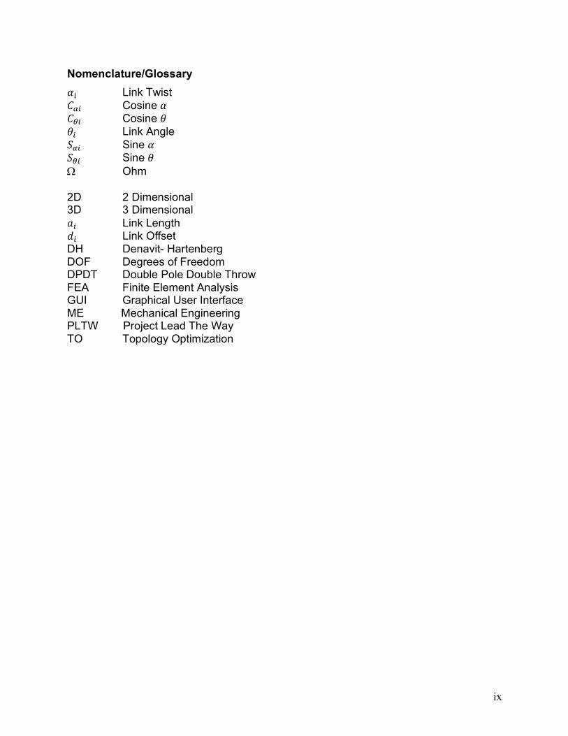
Nomenclature/Glossary 𝛼" Link Twist 𝐶$" Cosine 𝛼 𝐶%" Cosine 𝜃 𝜃" Link Angle 𝑆$" Sine 𝛼 𝑆%" Sine 𝜃 W Ohm 2D 2 Dimensional 3D 3 Dimensional 𝑎" Link Length 𝑑" Link Offset DH Denavit- Hartenberg DOF Degrees of Freedom DPDT Double Pole Double Throw FEA Finite Element Analysis GUI Graphical User Interface ME Mechanical Engineering PLTW Project Lead The Way TO Topology Optimization

x

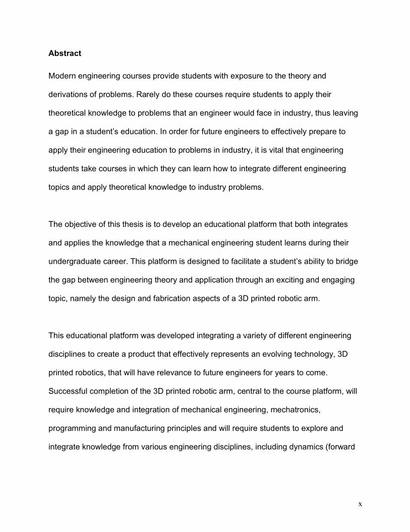
Abstract

Modern engineering courses provide students with exposure to the theory and

derivations of problems. Rarely do these courses require students to apply their

theoretical knowledge to problems that an engineer would face in industry, thus leaving

a gap in a student’s education. In order for future engineers to effectively prepare to

apply their engineering education to problems in industry, it is vital that engineering

students take courses in which they can learn how to integrate different engineering

topics and apply theoretical knowledge to industry problems.

The objective of this thesis is to develop an educational platform that both integrates

and applies the knowledge that a mechanical engineering student learns during their

undergraduate career. This platform is designed to facilitate a student’s ability to bridge

the gap between engineering theory and application through an exciting and engaging

topic, namely the design and fabrication aspects of a 3D printed robotic arm.

This educational platform was developed integrating a variety of different engineering

disciplines to create a product that effectively represents an evolving technology, 3D

printed robotics, that will have relevance to future engineers for years to come.

Successful completion of the 3D printed robotic arm, central to the course platform, will

require knowledge and integration of mechanical engineering, mechatronics,

programming and manufacturing principles and will require students to explore and

integrate knowledge from various engineering disciplines, including dynamics (forward

xi

and inverse kinematics), stress and strain analysis, FEA and topology optimization,

mechatronics, programing and manufacturing.

This developed educational platform promotes a learning experience in which students

have the opportunity to not only tinker and be creative but to develop an appreciation for

the application of a wide variety of engineering topics. The requirements of the project

also challenge students to adapt, evolve and develop their field-specific engineering

knowledge, while also developing their cross-functional engineering capabilities.

1

1.0 Introduction

1.1. Motivation

A thorough engineer is required to be inquisitive and think critically to anticipate

potential problems and thereby develop and implement preventive measures in

the design of artifacts. The robotic arm project proposed in this thesis provides a

powerful platform for the engineering student to develop and hone his/her

approach to problem solving and can apply engineering knowledge to the

development and an industry relevant problem.

This project develops an educational platform that will allow engineering students

to investigate, explore and integrate different engineering topics learned

throughout a student’s undergraduate career. This work is designed to motivate

and excite students about engineering topics through an engaging problem, as

well as encourage them to bridge the gap between theory and application.

Through the development of a 3D printed robotic arm students will explore topics

in the fields of mechanical engineering, manufacturing, mechatronics and

programming as well as how these topics overlap and intertwine.

This project outlines in detail the suggested steps an engineering student should

follow and the key decisions required during the developmental process. The

project discusses one possible functional robot that can be built through the

completion of the course, while maintaining the opportunity to develop creative

2

new designs. Through this educational platform, students have a rich opportunity

to learn, develop and innovate.

1.2. Literature Review

A number of other learning platforms that promote practical application of

engineering knowledge exist and are used for distinct purposes. For example,

the “Toy Design” course, developed at Purdue University and MIT, focuses on

the fundamentals of design, CAD systems, 3D printing and their integration.

Purdue University developed the course over 20 years ago as an innovative

approach for teaching CAD and prototyping for their Mechanical Engineering

students. The Purdue engineering leadership, hypothesized that the design and

prototyping project required by the “Toy Design” course would be an effective

way for students to gain a deeper knowledge of the CAD software through the

simulation of real-world applications. However, the focus of the course was

learning CAD, which was seen in the project results. Ultimately, the final projects

were geometrically and mechanically complex but lacked originality and

creativity. Therefore, ME444 at Purdue University was redesigned to focus less

on the CAD aspect and more on the design and creativity side through the

creation of the I8 Framework. I8 stands for inspiration, insight, ideation,

imagination, iteration, implementation and impact for innovation. The success of

the Purdue effort has been documented [1], although the toy design platform

does not include some of the topics that comprise the platform proposed in this

3

thesis, they are important for emphasizing a systems engineering perspective

that is critical for every new mechanical engineer.

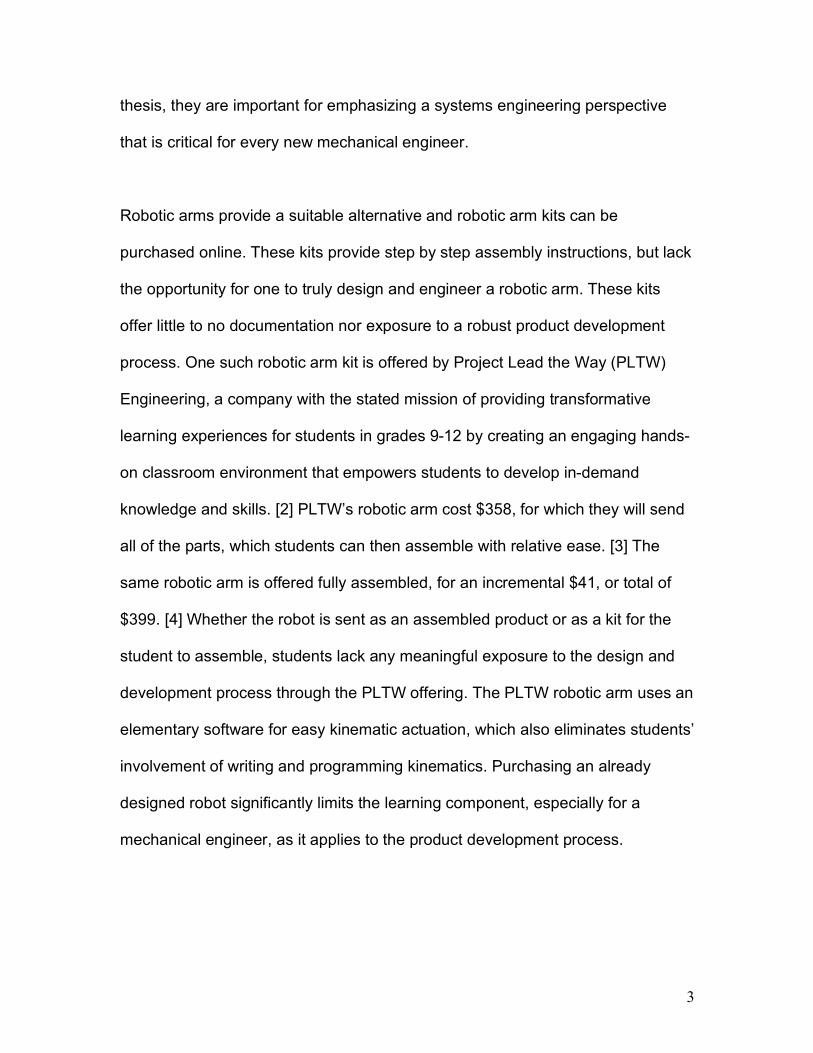
Robotic arms provide a suitable alternative and robotic arm kits can be

purchased online. These kits provide step by step assembly instructions, but lack

the opportunity for one to truly design and engineer a robotic arm. These kits

offer little to no documentation nor exposure to a robust product development

process. One such robotic arm kit is offered by Project Lead the Way (PLTW)

Engineering, a company with the stated mission of providing transformative

learning experiences for students in grades 9-12 by creating an engaging hands-

on classroom environment that empowers students to develop in-demand

knowledge and skills. [2] PLTW’s robotic arm cost $358, for which they will send

all of the parts, which students can then assemble with relative ease. [3] The

same robotic arm is offered fully assembled, for an incremental $41, or total of

$399. [4] Whether the robot is sent as an assembled product or as a kit for the

student to assemble, students lack any meaningful exposure to the design and

development process through the PLTW offering. The PLTW robotic arm uses an

elementary software for easy kinematic actuation, which also eliminates students’

involvement of writing and programming kinematics. Purchasing an already

designed robot significantly limits the learning component, especially for a

mechanical engineer, as it applies to the product development process.

4

The educational platform proposed here is similar in spirit to the “Toy Design”

course, but it involves a broader set of knowledge components and is further

“extensible” to cover engineering areas beyond those discussed in this thesis.

1.3. Objective

The primary objective of this thesis is to develop a platform that promotes

investigation, exploration, integration and application of different engineering

topics learned throughout a student’s undergraduate career. This is achieved

through the design and fabrication of a 3D printed robotic arm. The robotic arm is

actuated by stepper motors, connected to a computational platform and its

motion can be controlled via a user interface. By documenting the design and

construction procedures, I provide the framework for students to combine what

they learn in various classes across multiple engineering disciplines to create a

functional robot. A course developed based on this project could proceed the

senior capstone design courses that are the culmination of mechanical

engineering (ME) education in most ME undergraduate programs around the

country.

By designing and fabricating the 3D printed functional robot discussed in this

thesis, students will explore and integrate knowledge that includes:

- Coordinate Transformations

- Forward and Inverse Kinematics

- Design Considerations stemming from Loading conditions and Actuation

5

- 3D Modeling with CAD systems

- Stress and Strain Analysis

- Finite Element Analysis (FEA) and Topology Optimization (TO)

- Programming principles

- Mechatronics, and in particular actuation design and control

- Manufacturing Principles

1.4. Outline

The outline of this thesis is as follows:

- Chapter 2: Kinematics: Describes the necessary information in order to

write the forward and inverse kinematics for a kinematic manipulator

with 4 degrees of freedom.

- Chapter 3- Design of the Robotic Arm: Explores the product

development process. Specifically, the design process and

considerations, actuation and load analysis of the kinematic

manipulator, 3D modeling, finite element analysis and topology

optimization.

- Chapter 4- Mechatronics: Details the design of the necessary circuit

and double-pole double-throw switch needed for actuation of the

robotic arm.

- Chapter 5- Manufacturing: Discusses 3D printing technology as it

relates to manufacturing as well as its advantages and disadvantages.

6

- Chapter 6- Programming: Explains how the forward and inverse

kinematics are utilized to dictate movement using MATLAB and

Arduino.

- Chapter 7- Discussion: Summarizes the intentions of why the

educational platform was developed. Limitations of the robotic arm

developed in conjunction with this thesis are reviewed. Potential ways

of implementing of this project into a course and the vision for potential

future endeavors are investigated.

7

2.0 Kinematics

2.1. Objectives

This section describes the forward and inverse kinematics for a 3 DOF kinematic

manipulator with revolute joints. Kinematics, specifically, forward and inverse,

use joint angles or a coordinate location respectively to develop the mathematical

tools needed to describe the motion of the robotic arm.

2.2. Concepts

The following concepts will be used to define the forward and inverse kinematics

of my robotic arm:

- Degrees of Freedom (DOF)

- Coordinate Transformations

- Denavit-Hartenberg (DH) Parameters

- Workspace Analysis

- Robot Singularities

2.3. Background

2.3.1. Degrees of Freedom

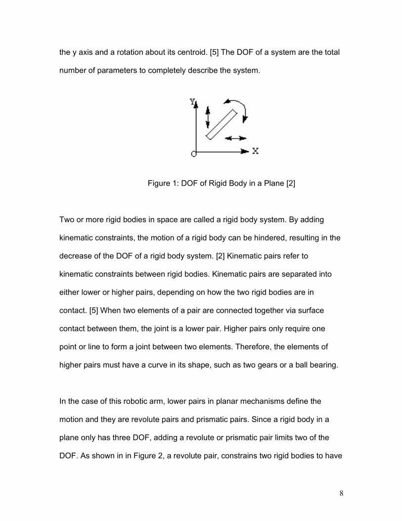
Degrees of freedom of a rigid body is defined as the number of its independent

movements. In order to determine the DOF of a rigid body, the number of distinct

movements must be considered. Figure 1, shows a rigid body in a two-

dimensional plane that has 3 DOF, translation along the x axis, translation along

8

the y axis and a rotation about its centroid. [5] The DOF of a system are the total

number of parameters to completely describe the system.

Figure 1: DOF of Rigid Body in a Plane [2]

Two or more rigid bodies in space are called a rigid body system. By adding

kinematic constraints, the motion of a rigid body can be hindered, resulting in the

decrease of the DOF of a rigid body system. [2] Kinematic pairs refer to

kinematic constraints between rigid bodies. Kinematic pairs are separated into

either lower or higher pairs, depending on how the two rigid bodies are in

contact. [5] When two elements of a pair are connected together via surface

contact between them, the joint is a lower pair. Higher pairs only require one

point or line to form a joint between two elements. Therefore, the elements of

higher pairs must have a curve in its shape, such as two gears or a ball bearing.

In the case of this robotic arm, lower pairs in planar mechanisms define the

motion and they are revolute pairs and prismatic pairs. Since a rigid body in a

plane only has three DOF, adding a revolute or prismatic pair limits two of the

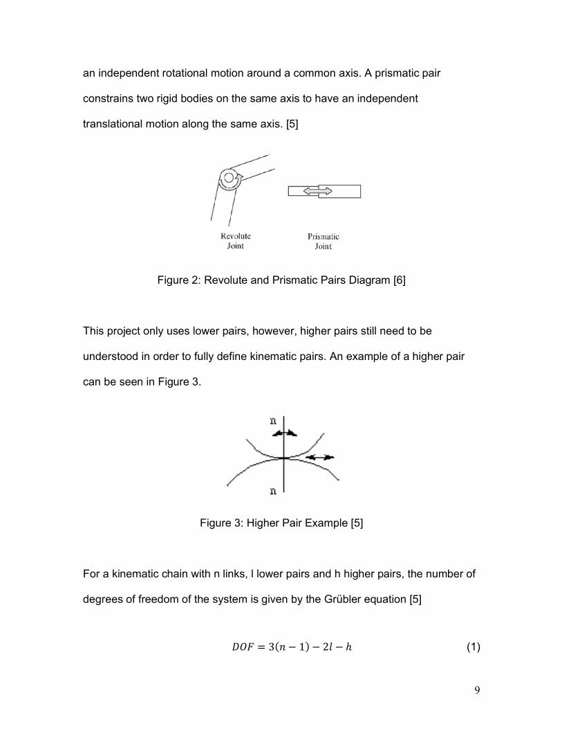
DOF. As shown in in Figure 2, a revolute pair, constrains two rigid bodies to have

9

an independent rotational motion around a common axis. A prismatic pair

constrains two rigid bodies on the same axis to have an independent

translational motion along the same axis. [5]

Figure 2: Revolute and Prismatic Pairs Diagram [6]

This project only uses lower pairs, however, higher pairs still need to be

understood in order to fully define kinematic pairs. An example of a higher pair

can be seen in Figure 3.

Figure 3: Higher Pair Example [5]

For a kinematic chain with n links, l lower pairs and h higher pairs, the number of

degrees of freedom of the system is given by the Grübler equation [5]

𝐷𝑂𝐹 = 3(𝑛 − 1) − 2𝑙 − ℎ (1)

10

2.3.2. Introduction to Coordinate Transformations

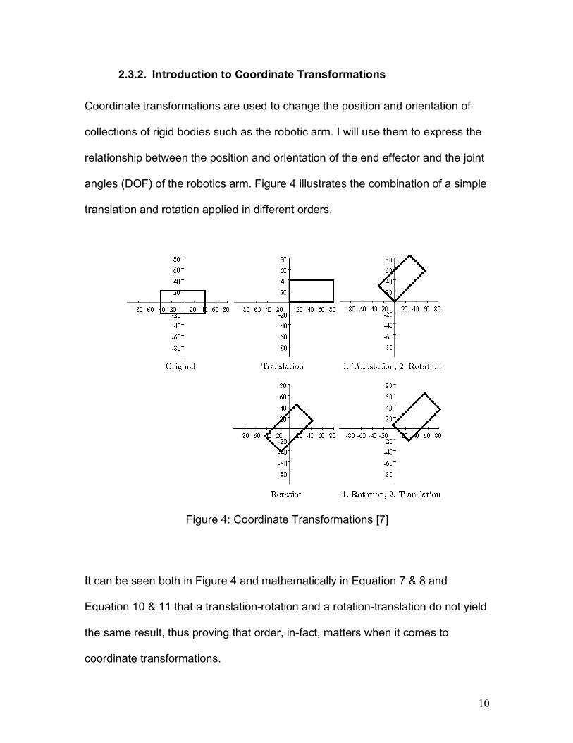
Coordinate transformations are used to change the position and orientation of

collections of rigid bodies such as the robotic arm. I will use them to express the

relationship between the position and orientation of the end effector and the joint

angles (DOF) of the robotics arm. Figure 4 illustrates the combination of a simple

translation and rotation applied in different orders.

Figure 4: Coordinate Transformations [7]

It can be seen both in Figure 4 and mathematically in Equation 7 & 8 and

Equation 10 & 11 that a translation-rotation and a rotation-translation do not yield

the same result, thus proving that order, in-fact, matters when it comes to

coordinate transformations.

11

One way coordinate transformations can be represented is using homogenous

coordinates. This allows translations and rotations both to be treated in the same

way as matrix multiplication. Additionally, since rotation matrices are

orthonormal, both orthogonal and unit vectors, it guarantees there is always an

inverse. If a function 𝑓 maps 𝑥 to 𝑦 then its inverse 𝑓:; will map 𝑦 to 𝑥.

Homogenous coordinates allow you to represent a 2-dimensional matrix

capturing the rotation in the plane in a space that has 3-dimensions. This can be

seen in the following equations.

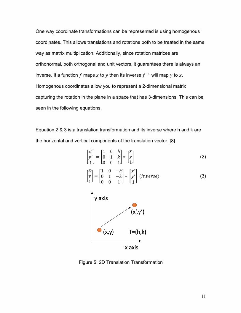
Equation 2 & 3 is a translation transformation and its inverse where h and k are

the horizontal and vertical components of the translation vector. [8]

<𝑥=𝑦=1> = <

1 0 ℎ0 1 𝑘0 0 1

> ∗ C𝑥𝑦1D (2)

C𝑥𝑦1D = <

1 0 −ℎ0 1 −𝑘0 0 1

> ∗ <𝑥=𝑦=1>(𝐼𝑛𝑣𝑒𝑟𝑠𝑒) (3)

Figure 5: 2D Translation Transformation

12

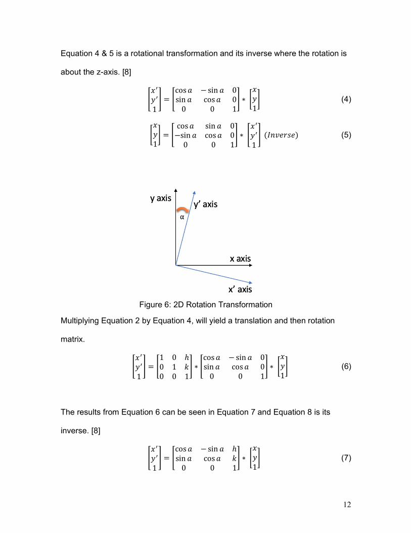
Equation 4 & 5 is a rotational transformation and its inverse where the rotation is

about the z-axis. [8]

<𝑥=𝑦=1> = <

cos𝑎 −sin 𝑎 0sin 𝑎 cos𝑎 00 0 1

> ∗ C𝑥𝑦1D (4)

C𝑥𝑦1D = <

cos𝑎 sin 𝑎 0−sin 𝑎 cos𝑎 00 0 1

> ∗ <𝑥=𝑦=1>(𝐼𝑛𝑣𝑒𝑟𝑠𝑒) (5)

Figure 6: 2D Rotation Transformation

Multiplying Equation 2 by Equation 4, will yield a translation and then rotation

matrix.

<𝑥=𝑦=1> = <

1 0 ℎ0 1 𝑘0 0 1

> ∗ <cos𝑎 − sin 𝑎 0sin 𝑎 cos𝑎 00 0 1

> ∗ C𝑥𝑦1D (6)

The results from Equation 6 can be seen in Equation 7 and Equation 8 is its

inverse. [8]

<𝑥=𝑦=1> = <

cos𝑎 −sin 𝑎 ℎsin 𝑎 cos𝑎 𝑘0 0 1

> ∗ C𝑥𝑦1D (7)

13

C𝑥𝑦1D = <

cos𝑎 sin 𝑎 −ℎ𝑐𝑜𝑠𝑎 − 𝑘𝑠𝑖𝑛𝑎−sin 𝑎 cos 𝑎 ℎ𝑠𝑖𝑛𝑎 − 𝑘𝑐𝑜𝑠𝑎0 0 1

> ∗ <𝑥=𝑦=1>(𝐼𝑛𝑣𝑒𝑟𝑠𝑒) (8)

On the other hand, if Equation 4 is multiplied by Equation 2, a rotation then

translation matrix will be yielded.

<𝑥=𝑦=1> = <

cos𝑎 −sin 𝑎 0sin 𝑎 cos𝑎 00 0 1

> ∗ <1 0 ℎ0 1 𝑘0 0 1

> ∗ C𝑥𝑦1D (9)

The results from Equation 9 can be seen in Equation 10 and Equation 11 is its

inverse. [8]

<𝑥=𝑦=1> = <

cos𝑎 −sin 𝑎 ℎ𝑐𝑜𝑠𝑎 − 𝑘𝑠𝑖𝑛𝑎sin 𝑎 cos𝑎 ℎ𝑠𝑖𝑛𝑎 + 𝑘𝑐𝑜𝑠𝑎0 0 1

> ∗ C𝑥𝑦1D (10)

C𝑥𝑦1D = <

cos𝑎 sin 𝑎 −ℎ−sin 𝑎 cos 𝑎 −𝑘0 0 1

> ∗ <𝑥=𝑦=1>(𝐼𝑛𝑣𝑒𝑟𝑠𝑒) (11)

Rigid body transformations are transformations that preserve the shape and size

of an object, such as translations and rotations. As it will be seen in Section 2.4,

multiplying any number of rigid body transformations, regardless of the type or

order will result in a rigid body transformation. Additionally, coordinate

transformations in 3D are represented by a 4-dimensional matrix but still follow

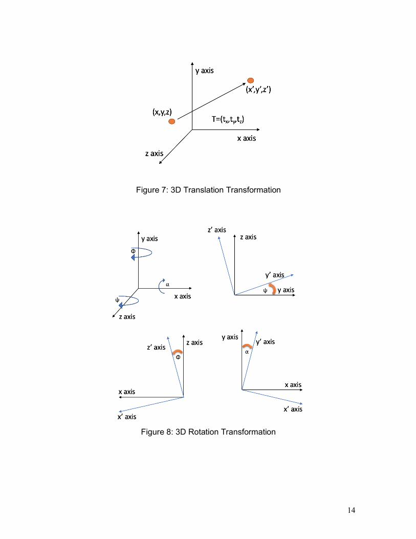
the same methodology as a 2-dimensional system. Figure 7 shows a 3D

translation and Figure 8 show a 3D rotation.

14

Figure 7: 3D Translation Transformation

Figure 8: 3D Rotation Transformation

15

2.4. Kinematics Formulation

Forward kinematics is the determination of the location of the end effector based

on specified joint angles and it always has only one solution. Inverse kinematics

is the determination of the angles of the joints based on a specified X, Y, Z

coordinate of the end effector. This is more complex than forward kinematics as

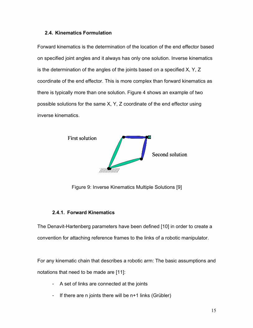
there is typically more than one solution. Figure 4 shows an example of two

possible solutions for the same X, Y, Z coordinate of the end effector using

inverse kinematics.

Figure 9: Inverse Kinematics Multiple Solutions [9]

2.4.1. Forward Kinematics

The Denavit-Hartenberg parameters have been defined [10] in order to create a

convention for attaching reference frames to the links of a robotic manipulator.

For any kinematic chain that describes a robotic arm: The basic assumptions and

notations that need to be made are [11]:

- A set of links are connected at the joints

- If there are n joints there will be n+1 links (Grübler)

16

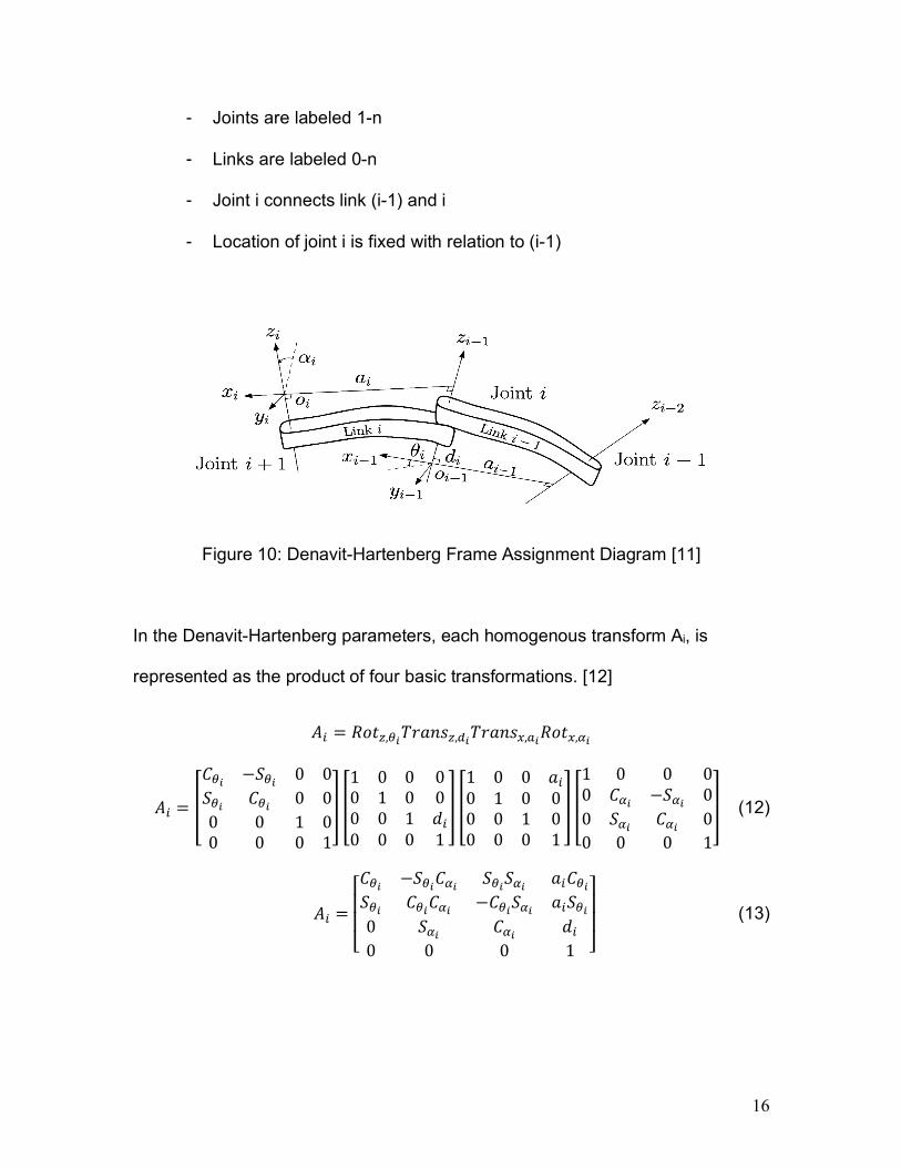
- Joints are labeled 1-n

- Links are labeled 0-n

- Joint i connects link (i-1) and i

- Location of joint i is fixed with relation to (i-1)

Figure 10: Denavit-Hartenberg Frame Assignment Diagram [11]

In the Denavit-Hartenberg parameters, each homogenous transform Ai, is

represented as the product of four basic transformations. [12]

𝐴" = 𝑅𝑜𝑡V,%X𝑇𝑟𝑎𝑛𝑠V,ZX𝑇𝑟𝑎𝑛𝑠[,\X𝑅𝑜𝑡[,$X

𝐴" = ]

𝐶%X −𝑆%X 0 0𝑆%X 𝐶%X 0 00 0 1 00 0 0 1

^ ]

1 0 0 00 1 0 00 0 1 𝑑"0 0 0 1

^ ]

1 0 0 𝑎"0 1 0 00 0 1 00 0 0 1

^ ]

1 0 0 00 𝐶$X −𝑆$X 00 𝑆$X 𝐶$X 00 0 0 1

^ (12)

𝐴" =

⎣⎢⎢⎡𝐶%X −𝑆%X𝐶$X 𝑆%X𝑆$X 𝑎"𝐶%X𝑆%X 𝐶%X𝐶$X −𝐶%X𝑆$X 𝑎"𝑆%X0 𝑆$X 𝐶$X 𝑑"0 0 0 1 ⎦

⎥⎥⎤ (13)

17

Where ai, ai, di, θi are link length, link twist, link offset and joint angle respectively

and the subscript i, is associated with link i and joint i. Additionally, 𝐶%", 𝐶$", 𝑆%",

𝑆$" are respectively representing the cosine and sine function.

Matrix Ai represents a function of a single variable, due to three of the four

variables being constant for a given link, while the fourth parameter, θi for a

revolute joint is the joint variable. [12]

In Equation 12 & 13, Ai, is a product of a rotation-translation-translation-rotation

matrix. Using the frame assignment in Figure 10, first a rotation of ai, the link

twist, about the x-axis is taking place. Next, a translation of ai, the link length, on

the x-axis follows. Then a second translation of di, the link offset, on the z-axis is

occurring. Finally, the coordinate systems of Zi and Zi-1 are aligned and the last

rotation is on the z-axis is the joint variable. This alignment is important because

Ai allows you to convert coordinates between coordinate systems as well as

move points in the same coordinate system.

2.4.2. Inverse Kinematics

Inverse kinematics is complex, however, in the case of manipulators with six

joints with the last three joints intersecting at a point, decoupling will simplify the

problem. The inverse kinematics will be decoupled into inverse position

kinematics and inverse orientation kinematics. In the case of the robotic arm

discussed in this thesis, the inverse orientation kinematics is simplified to only

18

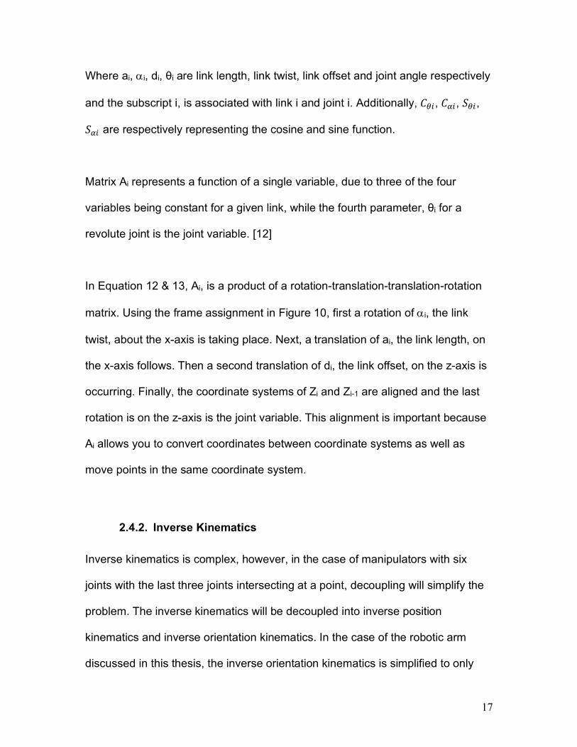
one joint rather than three. The following equations can be used to determine the

angles for the desired end effector location of the inverse position kinematics.[12]

𝜃; = 𝐴𝑡𝑎𝑛2(𝑋f, 𝑦f) (14)

𝑐𝑜𝑠𝜃g =hijki:\ii:\li

m\i\l= [n

ijoni:ZijVni:\ii:\li

m\i\l≔ 𝐷

𝜃g = 𝐴𝑡𝑎𝑛(𝐷,±√1 − 𝐷m) (15)

𝜃m = 𝐴𝑡𝑎𝑛(𝑟, 𝑠) − 𝐴𝑡𝑎𝑛(𝑎m + 𝑎g𝑐g, 𝑎g𝑠g) =

𝐴𝑡𝑎𝑛st𝑥fm + 𝑦fm − 𝑑m, 𝑧fv − 𝐴𝑡𝑎𝑛(𝑎m + 𝑎g𝑐g, 𝑎g𝑠g) (16)

In the above equations θ3 has two corresponding solutions respectively showing

the elbow up vs elbow down configuration.

Figure 11: Robotic Configuration for Inverse Kinematic [12]

19

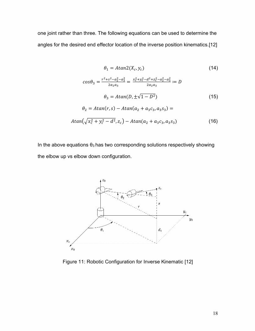
Inverse kinematics typically has more than one solution which can lead to

possible difficulties. Robot singularities fall under this category. Figure 12 shows

an example of a robot singularity when 𝑠𝑖𝑛𝜃 = wx the range of motion of the

output is within the workspace, however, the output can undergo infinitesimal

motion, even if the input is locked. Additionally, along the x axis the mechanism

cannot resist a force applied at the output. [13]

Figure 12: Planar RRRP Mechanism [13]

2.5. Key Questions

Some key questions and concepts to consider when writing the forward and

inverse kinematics are:

Concepts:

- Robot singularities

o A condition in which a robotic manipulator loses one or more

DOF and changes in the joint variable does not result in a

change of the end effector location and orientation.

20

- Accuracy & Repeatability

o Accuracy

§ The precision of a displacement value

o Repeatability

§ How precisely a robot returns to a specified point

- Workspace

o A set of all possible points that the robotic arm can reach

Questions:

- What is a workspace? How can it be computed? How much of the

workspace do you want active?

- Kinematics does not involve dynamics (loads). How do the loads and

the load distribution change/impact kinematics?

21

3.0 Design of the Robotic Arm

3.1. Objectives

This section covers the design process of the robotic arm, from design

considerations to topologically optimized links.

3.2. Concepts

The following concepts need to be part of any successful design of a robotic arm:

- Design Requirements

- Actuation

- Loads

- Load Capacity

- Material Properties

- Stress and Strain Analysis

- 3D Modeling

- Finite Element Analysis

- Topology Optimization

3.3. Background

3.3.1. Design Requirements

The following properties were selected for the robotic arm discussed in this

thesis. However, as this project is a developmental platform, the properties

selected are by no means a required mandate. Properties can and should be

modified by students based on their final goal.

22

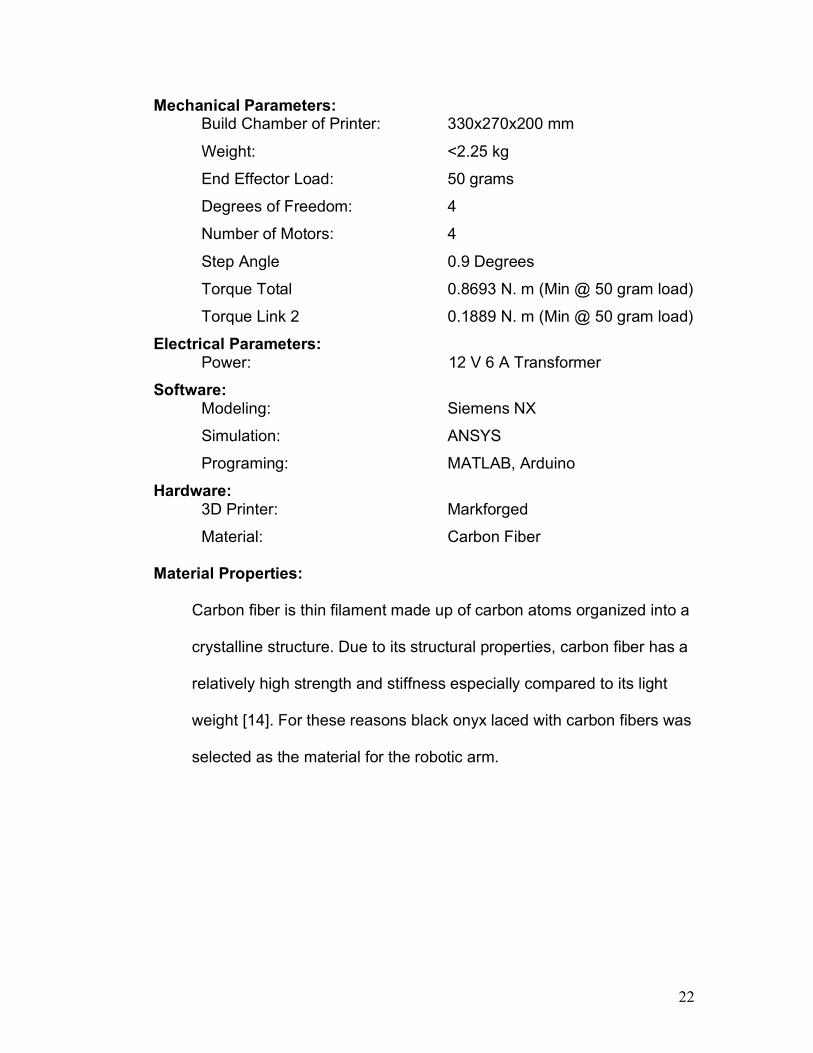
Mechanical Parameters: Build Chamber of Printer: 330x270x200 mm

Weight: <2.25 kg

End Effector Load: 50 grams

Degrees of Freedom: 4

Number of Motors: 4

Step Angle 0.9 Degrees

Torque Total 0.8693 N. m (Min @ 50 gram load)

Torque Link 2 0.1889 N. m (Min @ 50 gram load)

Electrical Parameters: Power: 12 V 6 A Transformer

Software: Modeling: Siemens NX

Simulation: ANSYS

Programing: MATLAB, Arduino

Hardware: 3D Printer: Markforged

Material: Carbon Fiber

Material Properties:

Carbon fiber is thin filament made up of carbon atoms organized into a

crystalline structure. Due to its structural properties, carbon fiber has a

relatively high strength and stiffness especially compared to its light

weight [14]. For these reasons black onyx laced with carbon fibers was

selected as the material for the robotic arm.

23

Measurement Value

Density ( yfzi) 1.4

Young’s Modulus (GPa) 54

Poisson Ratio 0.35

Bulk Modulus (GPa) 60

Shear Modulus (GPa) 20

Tensile Strength (MPa) 800

Flexural Strength (MPa) 470

Table 1: Black Onyx Carbon Fiber Properties [15]

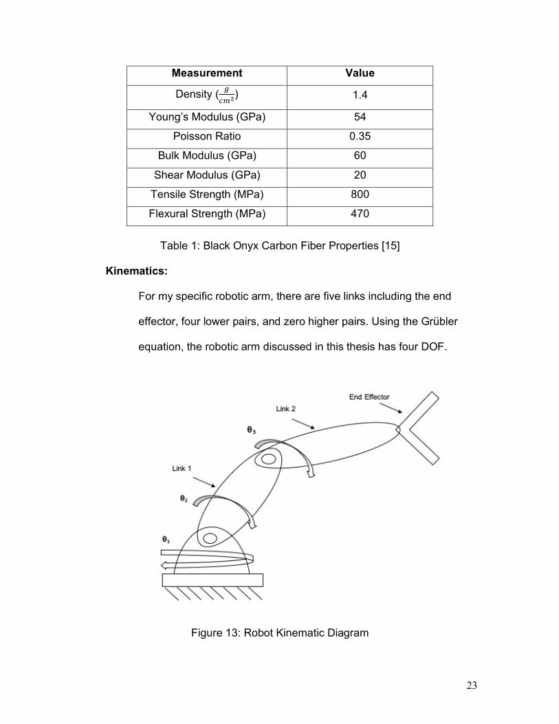
Kinematics:

For my specific robotic arm, there are five links including the end

effector, four lower pairs, and zero higher pairs. Using the Grübler

equation, the robotic arm discussed in this thesis has four DOF.

Figure 13: Robot Kinematic Diagram

24

3.3.2. Design Considerations

Throughout this project there are several design considerations. This section will

provide a brief overview of some of these design related considerations and they

are further expanded upon in following sections. These considerations include

but are not limited to: degrees of freedom, size, weight, loads, type of motors and

their placement, material selection and capability of the 3D printer. With each

DOF added to the system, the complexity increases with regard to the forward

and inverse kinematics, effecting programming and circuit layout, as well as the

overall weight of the system, the distribution of torque, and assembly. The size of

the robot needs to be taken into consideration because it directly correlates with

the weight of the robot and thus the amount of torque needed to move the

system. The load that the system can lift affects all of the physical parameters,

especially the finite element analysis, topology optimization and power of the

motors. Based on the aforementioned decisions, the center of mass and weight

for each component of the system will dictate what motors will have to be used.

The mounting location of the motors is an important consideration as it affects

the weight distribution for the robotic arm and therefore the loads that the motors

will have to sustain. The weight distribution also affects the dynamic properties of

the robot and the repeatability. Positioning the motors closer to the base allows

the weight of the motors to not affect the actuation with regards to torque;

however, the complexity of the transmission of motion to the links increases in

relation to motor base proximity. Furthermore, the precision and accuracy of the

motor needs to be factored as a key contributor to the repeatability of the motion

25

of the arm. The workspace needs to be taken into consideration as it is the set of

all possible points that the end effector can reach. Additionally, it is important to

determine whether to use a servo motor or stepper motor, as each motor has

different benefits and disadvantages. Equally important, is material selection,

which will dictate not only the stiffness of the robot but also the weight

distribution. Finally, the capabilities of the 3D printer will dictate the

manufacturing variations and related assembly and functional issues for the

whole system.

3.3.3. Introduction to Topology Optimization Theory

Topology optimization is a method in which a material layout is mathematically

optimized based on specific design specifications, boundary conditions and loads

while the design remains structurally intact. Topology optimization uses a finite

element analysis to evaluate the performance of a shape, such as using a von

Mises stress equivalent to determine the stresses on a shape. Then, based on

the finite element analysis a topology optimization can be run to minimize mass

and maximize performance.

Topology optimization is very useful as it can render complex shapes in a design

space. However, it may give rise to problematic issues in the manufacturing

stage such as not being able to remove support structures. The geometry

resulting for a typical topology optimization algorithm must be modified to fit the

capabilities of the manufacturing process in use. This, in turn, moves the design

26

away from the optimum, often by a significant degree. Additive manufacturing

can be used to fabricate very complex geometries with relatively little additional

cost. Additive manufacturing fits naturally as a manufacturing process for shapes

that have been designed via topology optimization.

Topology optimizing a part for manufacturing without setting constraints will yield

an organic looking shape. However, the solutions output by some commercial

topology optimization software need to be post processed so that the object

boundaries fit the manufacturing process without introducing unnecessary stress

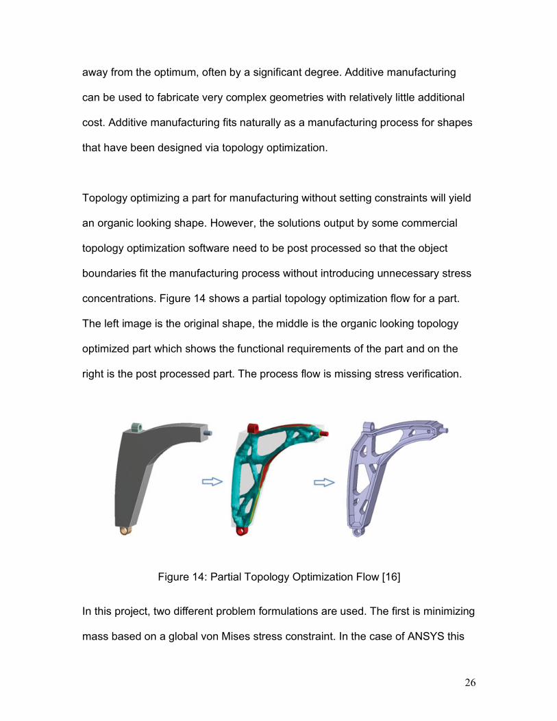
concentrations. Figure 14 shows a partial topology optimization flow for a part.

The left image is the original shape, the middle is the organic looking topology

optimized part which shows the functional requirements of the part and on the

right is the post processed part. The process flow is missing stress verification.

Figure 14: Partial Topology Optimization Flow [16]

In this project, two different problem formulations are used. The first is minimizing

mass based on a global von Mises stress constraint. In the case of ANSYS this

27

global value is an average. This methodology evaluates the stress on the shape

and eliminates as much mass as possible without violating stress. However,

sometimes designs are not stress driven if the loads are small compared to the

stiffness of the material. In light of this, a second formulation was used,

compliance minimization subject to a mass fraction constraint. Minimizing

compliance is equivalent to maximizing stiffness.

An important consideration in topology optimization is the selection of a mesh

size. A fine mesh will yield a more detailed design, but it takes longer to run

because of the finite element analysis. A coarse mesh may not yield the most

optimal shape. Therefore, the size of the mesh should be carefully selected to

balance these two aspects.

3.4. Design Formulation

3.4.1. Actuation and Load Analysis

The key decision factors for motor selection include weight, torque, type of motor

and its placement. Servo motors receive current only when they are required to

move or hold a load. Servo motors can provide peak torque several times higher

than the maximum of a continuous motor torque for acceleration. Alternatively,

stepper motors operate in an open loop constant current mode which creates a

significant amount of heat in both the motor and the drive as they operate.

Additionally, when there is no encoder, it can allow for a cost saving, when there

is an encoder it can also be controlled in a closed loop mode. Stepper motors

28

have more poles than servo motors which allows them to have more torque at

lower speeds, however the increased speed results in torque degradation. [17]

Stepper motors offer a few benefits compared to servo motors. They are easier

to commission, simpler to maintain and are less expensive. Stepper motors are

stable at rest and hold their position with a dynamic load without any fluctuation.

Servo motors are excellent when high torque at high speeds is required or when

a high dynamic response is required. Stepper motors are excellent for low to

medium acceleration rates and for high holding torque. [17]

For the motor location, it is necessary to consider how the motors will be

mounted (i.e. at the joints or will they need to transfer power via a gear system).

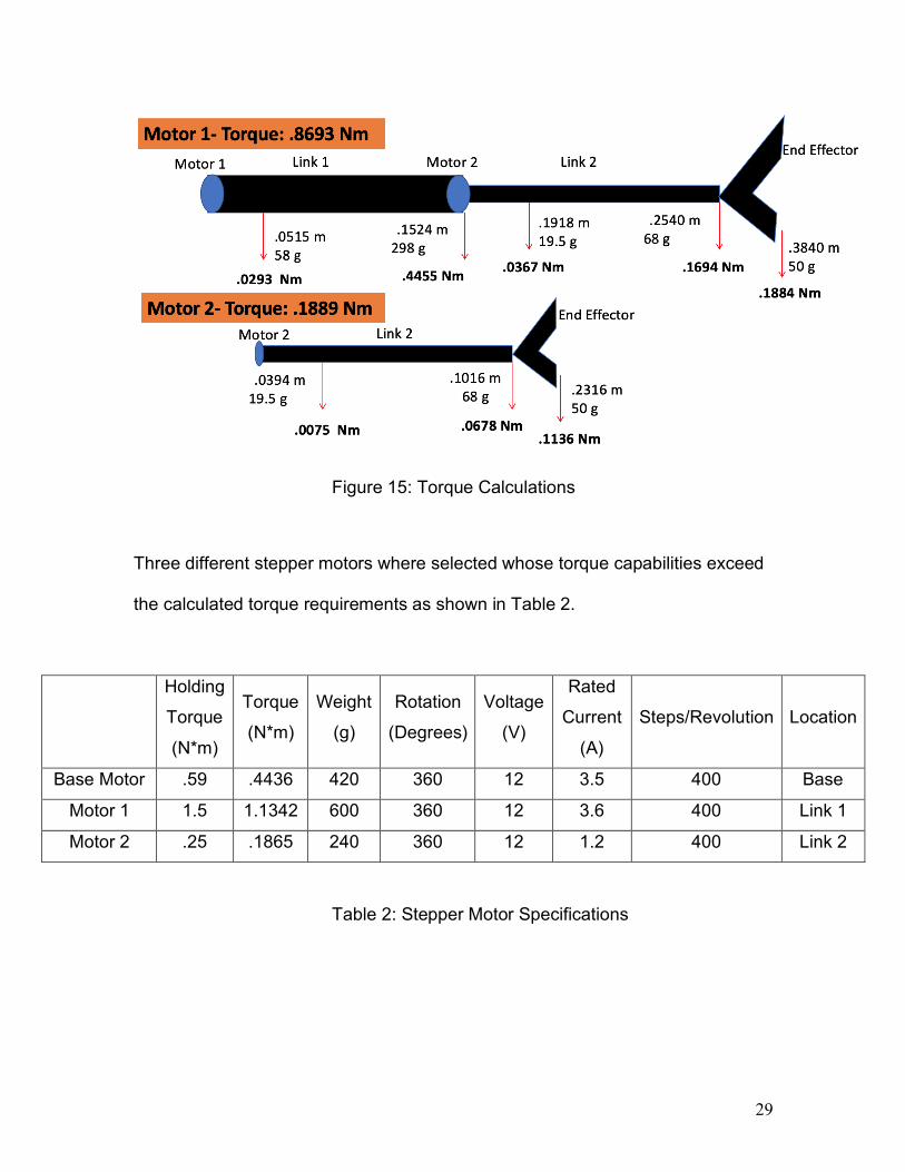
Figure 15 shows schematically the kinematic manipulator: the top figure shows

the loads that need to be considered to size Motor 1. The first arrow from the left

is the weight of link 1 at the center of mass of link 1; the second arrow is at the

end of link 1 and is the weight of the two bearings and motor 2. The third arrow is

the weight of link 2 at the center of mass for link 2. The fourth arrow is at the end

of link 2 and is the weight of the end effector. In reality, the center of mass of the

end effector is not at the end of link 2, however, it is acceptable due to

accounting for the load, the last arrow, being at the tip of the end effector. Similar

calculations are shown for motor 2 in Figure 15. It is important to point out that

this configuration shows the worst-case scenario with regards to the necessary

torque required as the arm is completely extended.

29

Figure 15: Torque Calculations

Three different stepper motors where selected whose torque capabilities exceed

the calculated torque requirements as shown in Table 2.

Holding

Torque

(N*m)

Torque

(N*m)

Weight

(g)

Rotation

(Degrees)

Voltage

(V)

Rated

Current

(A)

Steps/Revolution Location

Base Motor .59 .4436 420 360 12 3.5 400 Base

Motor 1 1.5 1.1342 600 360 12 3.6 400 Link 1

Motor 2 .25 .1865 240 360 12 1.2 400 Link 2

Table 2: Stepper Motor Specifications

30

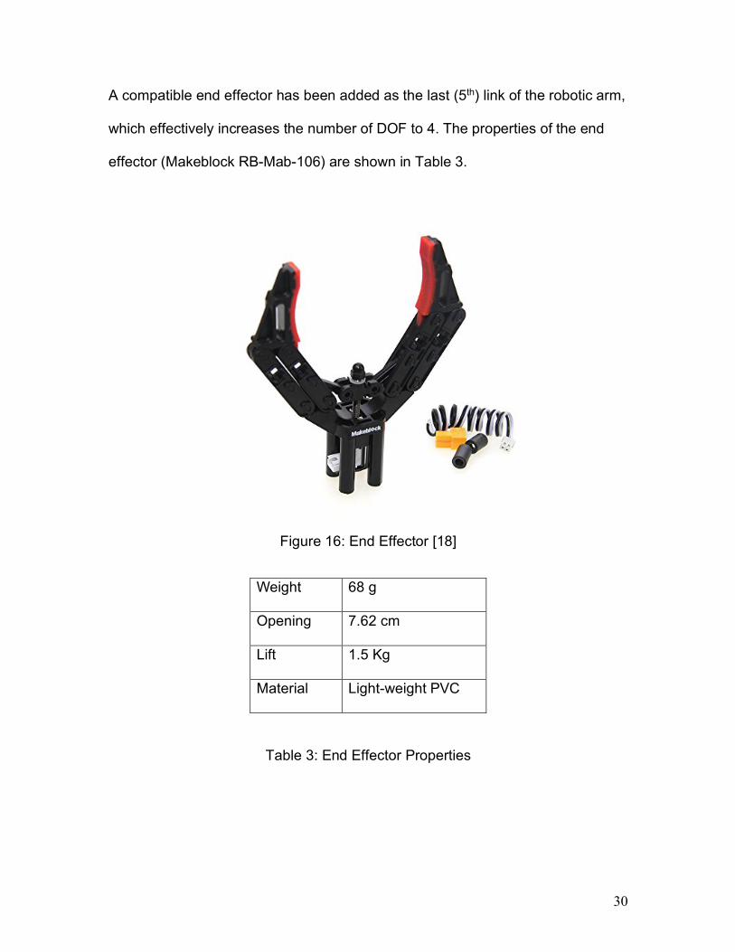
A compatible end effector has been added as the last (5th) link of the robotic arm,

which effectively increases the number of DOF to 4. The properties of the end

effector (Makeblock RB-Mab-106) are shown in Table 3.

Figure 16: End Effector [18]

Weight 68 g

Opening 7.62 cm

Lift 1.5 Kg

Material Light-weight PVC

Table 3: End Effector Properties

31

3.4.2. Topology Optimization

3.4.2.1. 3D Modeling

Knowledge of 3D modeling is critical to the design process. Siemens NX was

used for this project. Each part was designed to improve and simplify the design.

The starting geometry (design space) for the topology optimization step

influences the solutions that are being determined. Selecting a design space that

is too small may eliminate some of the possible solutions. However, the larger

the design space, the higher the computational cost of the topology optimization

step.

Several design considerations are factored into the development. For assembly,

it is necessary to consider how the system will be assembled (i.e. is it a feasible

simple design). For loads and material properties it is necessary to consider how

big of a load the selected material will support. Additionally, since the system will

be 3D printed, part shrinkage must be considered.

3.4.2.2. Topology Optimization Simulation

The optimization problem was set up to minimize mass with stress and stiffness

as constraints. A 10 N load was selected for the base rotation and a 5 N load

was selected for both for Link 1 and Link 2. These numbers were decided based

on the load the end effector is supposed to support. A factor of safety of 1.5 was

32

imposed on the stresses. The tensile strength of the material is 800 MPa and so

the stress constraint in the optimization is 533 MPa.

The process by which each part was optimized is as follows. First, the design

region was uploaded to ANSYS, and the material was defined in the settings.

Then, the loads and the fixed displacement supports were applied in the

appropriate locations. Next the design region is meshed. Note this is not the final

size mesh that will be used, as it will be refined later.

Now that the part is set up, a FEA can be run, to see how the loads affect the

shape, for instance, to determine the von Mises stresses. At this point, the mesh

should continue to be refined until the stress values start to converge to a value

where the stresses do not change significantly. The FEA results can be found in

Section 3.5. Next, the topology optimization problem is set up and run. Using the

results from this optimization, post processing is done on each part in NX. The

stress level was checked using the original setup and re-running a finite element

analysis. In general, less material will increase stress, however, if there are no

stress concentratives in the design region and the maximum stress is within the

factor of safety, the part is structurally feasible. If the stress exceeds the

allowable stresses, the part needs to be modified until the stresses are in the

allowable range. The results from the topology optimization can be found in

Section 3.5.

33

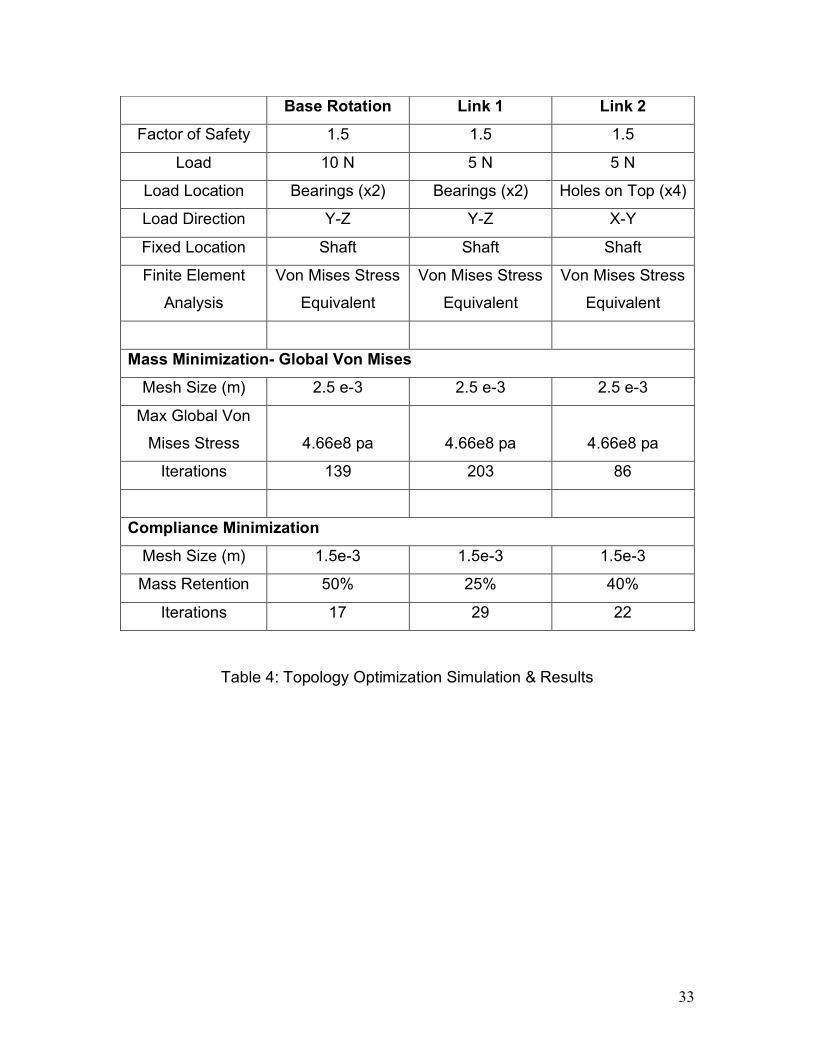
Table 4: Topology Optimization Simulation & Results

Base Rotation Link 1 Link 2 Factor of Safety 1.5 1.5 1.5

Load 10 N 5 N 5 N

Load Location Bearings (x2) Bearings (x2) Holes on Top (x4)

Load Direction Y-Z Y-Z X-Y

Fixed Location Shaft Shaft Shaft

Finite Element

Analysis

Von Mises Stress

Equivalent

Von Mises Stress

Equivalent

Von Mises Stress

Equivalent

Mass Minimization- Global Von Mises

Mesh Size (m) 2.5 e-3 2.5 e-3 2.5 e-3

Max Global Von

Mises Stress 4.66e8 pa 4.66e8 pa 4.66e8 pa

Iterations 139 203 86

Compliance Minimization

Mesh Size (m) 1.5e-3 1.5e-3 1.5e-3

Mass Retention 50% 25% 40%

Iterations 17 29 22

34

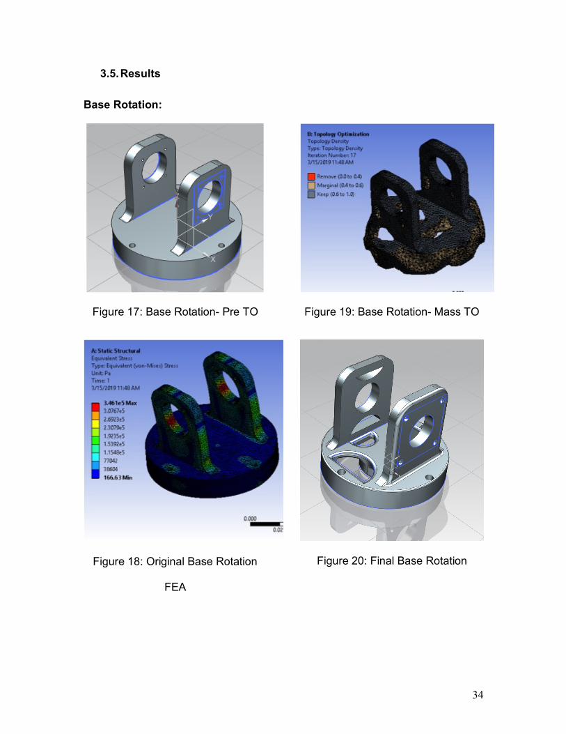
3.5. Results

Base Rotation:

Figure 17: Base Rotation- Pre TO

Figure 18: Original Base Rotation

FEA

Figure 19: Base Rotation- Mass TO

Figure 20: Final Base Rotation

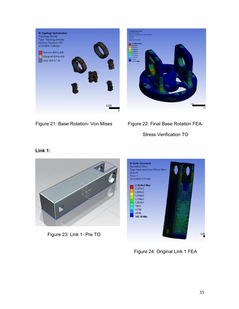
35

Figure 21: Base Rotation- Von Mises

Figure 22: Final Base Rotation FEA-

Stress Verification TO

Link 1:

Figure 23: Link 1- Pre TO

Figure 24: Original Link 1 FEA

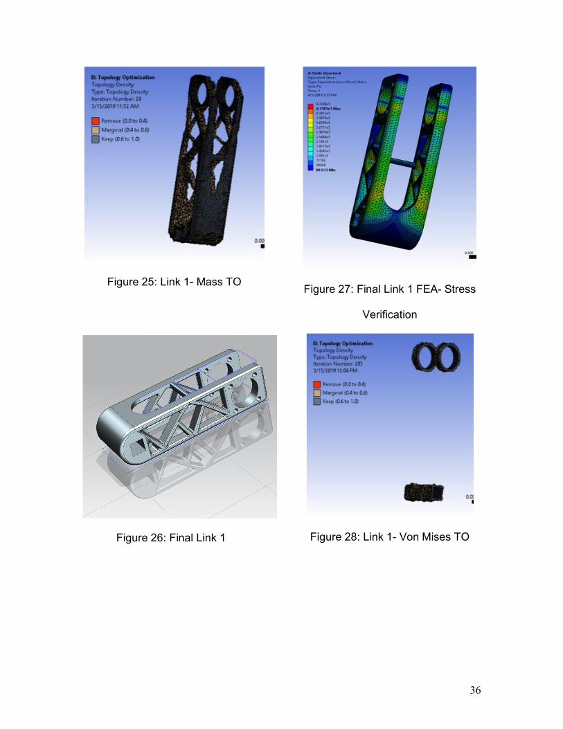
36

Figure 25: Link 1- Mass TO

Figure 26: Final Link 1

Figure 27: Final Link 1 FEA- Stress

Verification

Figure 28: Link 1- Von Mises TO

37

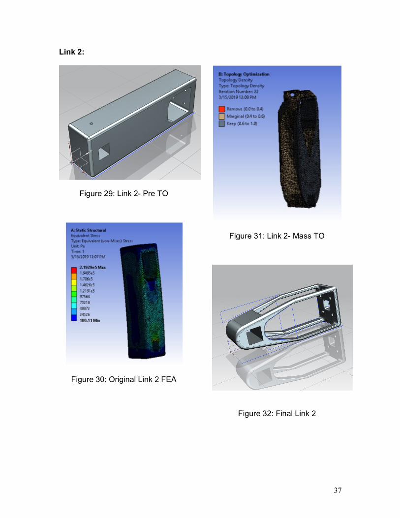
Link 2:

Figure 29: Link 2- Pre TO

Figure 30: Original Link 2 FEA

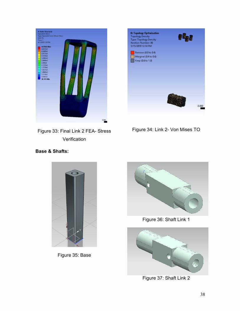
Figure 31: Link 2- Mass TO

Figure 32: Final Link 2

38

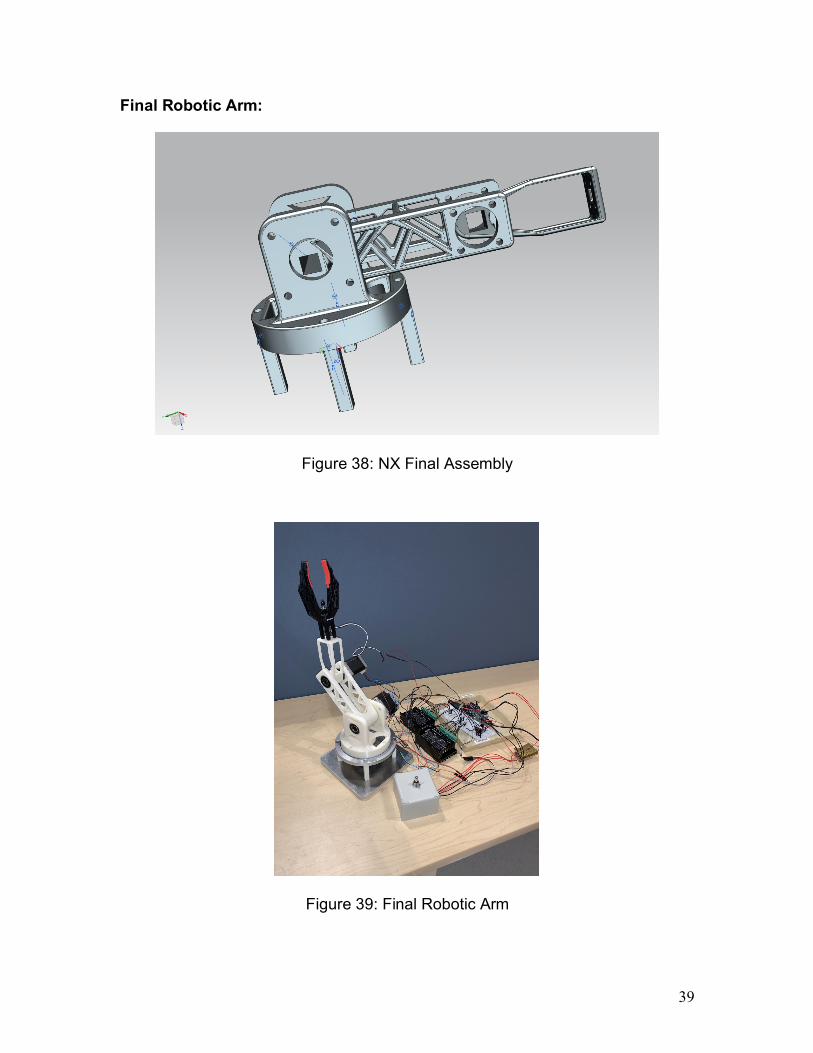
Figure 33: Final Link 2 FEA- Stress

Verification

Figure 34: Link 2- Von Mises TO

Base & Shafts:

Figure 35: Base

Figure 36: Shaft Link 1

Figure 37: Shaft Link 2

39

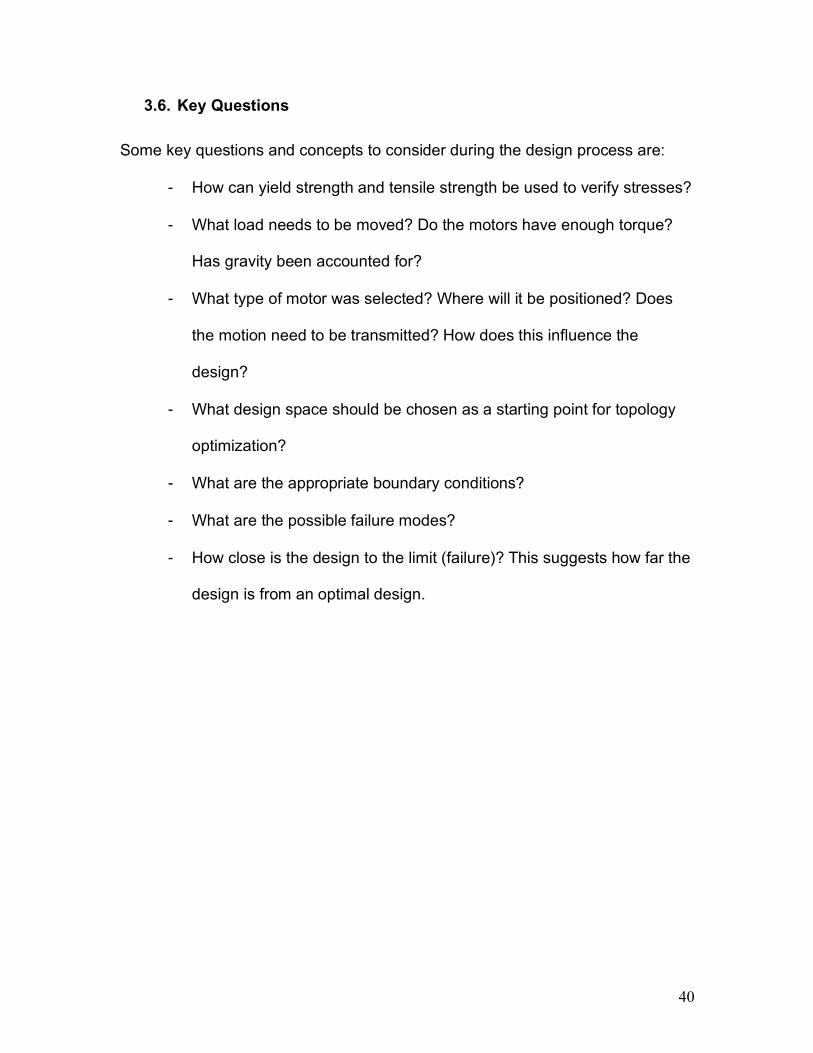
Final Robotic Arm:

Figure 38: NX Final Assembly

Figure 39: Final Robotic Arm

40

3.6. Key Questions

Some key questions and concepts to consider during the design process are:

- How can yield strength and tensile strength be used to verify stresses?

- What load needs to be moved? Do the motors have enough torque?

Has gravity been accounted for?

- What type of motor was selected? Where will it be positioned? Does

the motion need to be transmitted? How does this influence the

design?

- What design space should be chosen as a starting point for topology

optimization?

- What are the appropriate boundary conditions?

- What are the possible failure modes?

- How close is the design to the limit (failure)? This suggests how far the

design is from an optimal design.

41

4.0 Mechatronics

4.1. Objectives

This section will describe the circuit that will actuate the movement of the

kinematic manipulator.

4.2. Concepts

The following concepts need to be part of any successful design of a circuit for

actuation:

- Ohms law

- Current

- Voltage

- Resistors

- Capacitors

- Amplifiers

- Soldering

- Using a Multimeter

- Reading wiring schematics

4.3. Background

4.3.1. Ohm’s Law

Knowledge of Ohm’s law, the relationship between voltage, current, and

resistance, is essential to mechatronics. Voltage is the difference in charge

between two points. Current is the rate at which charge is flowing. Resistance is

42

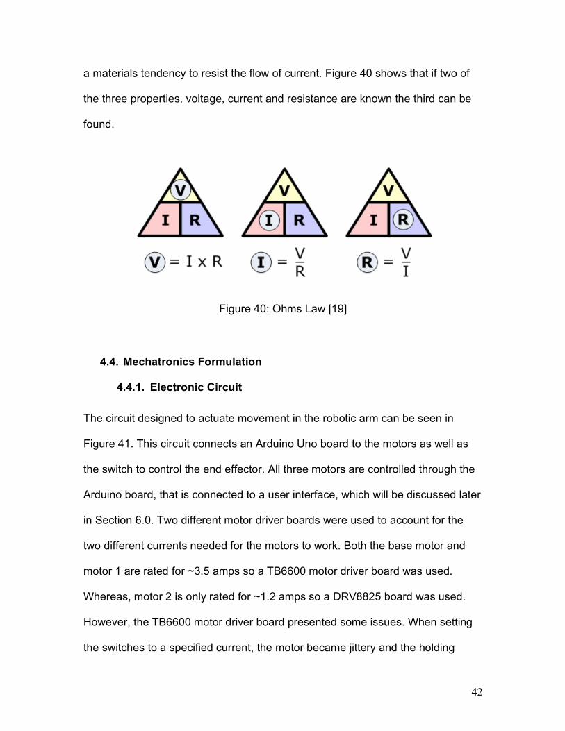
a materials tendency to resist the flow of current. Figure 40 shows that if two of

the three properties, voltage, current and resistance are known the third can be

found.

Figure 40: Ohms Law [19]

4.4. Mechatronics Formulation

4.4.1. Electronic Circuit

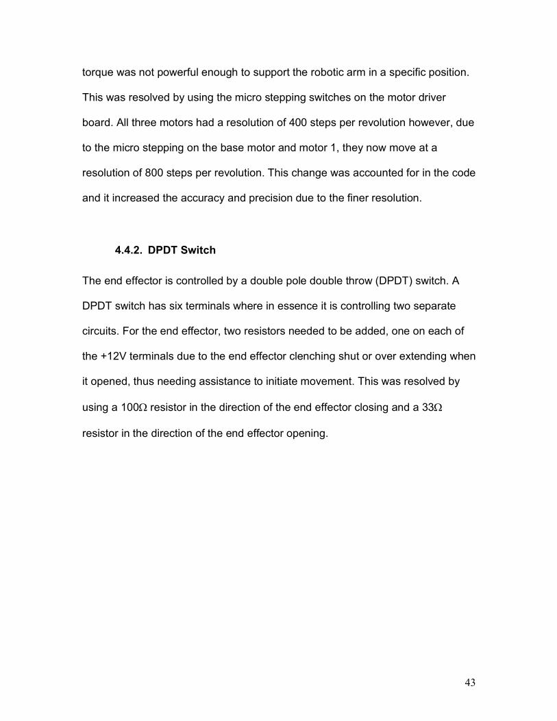
The circuit designed to actuate movement in the robotic arm can be seen in

Figure 41. This circuit connects an Arduino Uno board to the motors as well as

the switch to control the end effector. All three motors are controlled through the

Arduino board, that is connected to a user interface, which will be discussed later

in Section 6.0. Two different motor driver boards were used to account for the

two different currents needed for the motors to work. Both the base motor and

motor 1 are rated for ~3.5 amps so a TB6600 motor driver board was used.

Whereas, motor 2 is only rated for ~1.2 amps so a DRV8825 board was used.

However, the TB6600 motor driver board presented some issues. When setting

the switches to a specified current, the motor became jittery and the holding

43

torque was not powerful enough to support the robotic arm in a specific position.

This was resolved by using the micro stepping switches on the motor driver

board. All three motors had a resolution of 400 steps per revolution however, due

to the micro stepping on the base motor and motor 1, they now move at a

resolution of 800 steps per revolution. This change was accounted for in the code

and it increased the accuracy and precision due to the finer resolution.

4.4.2. DPDT Switch

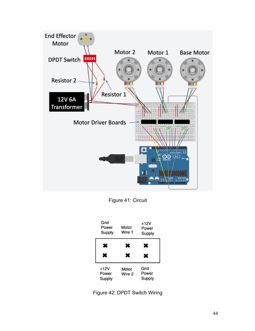
The end effector is controlled by a double pole double throw (DPDT) switch. A

DPDT switch has six terminals where in essence it is controlling two separate

circuits. For the end effector, two resistors needed to be added, one on each of

the +12V terminals due to the end effector clenching shut or over extending when

it opened, thus needing assistance to initiate movement. This was resolved by

using a 100W resistor in the direction of the end effector closing and a 33W

resistor in the direction of the end effector opening.

44

Figure 41: Circuit

Figure 42: DPDT Switch Wiring

45

4.5. Key Questions

Some key questions and concepts to consider during the circuit design and build

process are:

- What effect do resistors and capacitors have on the system?

- How can voltage and current be verified to ensure the system will not

fry?

- Why does wire thickness need to be considered?

- How do motors and amplifiers relate with torque and current?

46

5.0 Manufacturing

5.1. Objectives

This section will cover the manufacturing issues of 3D printing as they relate to

the functionality of the 3D printed components.

5.2. Concepts

The following concepts need to be part of the design stage to successfully

manufacture parts for assembly using a 3D printer and in particular, the

Markforged:

- Material properties

- Material shrinkage

- Printer selection

- Assembly

5.3. Background

As engineers, we design an array of structures, devices, products and systems,

however, each must be designed for a specific manufacturing process, with

consideration for fabrication challenges, production cost and quality control.[20]

The nature of additive manufacturing is changing the manufacturing field.

Additive manufacturing uses a layerwise approach which enables incomparable

complex geometries. The setup process is relatively simple, which reduces the

47

need for human involvement. Another benefit of additive manufacturing systems

is that they are relatively low cost. [20] In Section 5.4, the advantages and

disadvantages of 3D printing will be evaluated.

5.4. Manufacturing Formulation

Additive manufacturing opens the design space and removes many of the

conventional design constraints imposed by other methods. Rather than

designing for manufacturing, where manufacturing capabilities limit the design,

additive manufacturing is manufacturing for design where the design limits the

manufacturing. This is due to the ability to produce geometries that were

previously not possible.[20]

The layer-by layer fabrication of additive manufacturing allows for benefits such

as lightweight structures, internal cooling passages, better product performance,

reduced manufacturing lead-time and shorter product development time. Additive

manufacturing has a reduced cost due to the decrease in setup time, elimination

of tooling costs and reduced material waste. [20]

Additive manufacturing has slow build rates and parts can only be printed one at

a time. As a result, other manufacturing methods may be more optimal. The

layered print methodology of additive manufacturing offers many benefits;

however, it can also lead to defects in the product due to misaligned or skipped

layers. The material choice is often limited, and the build space is restricted to

48

the printers build chamber. Therefore, large pieces must be divided into sections

and assembled during post processing. Material shrinkage must be considered

as it is affected differently depending on several factors such as the printer, the

material as it is not isotropic, and the direction in which it is printed. Material

shrinkage also affects the tolerances, specifically there are deviations in both the

shape and locations of holes. Additionally, using a composite material such as

carbon fiber, creates issues with assembly. Should a screw be needed to fasten

parts together, the screw will not be able to grip onto the material as it will simply

strip any thread in the material, thus creating the need for a threaded heat set

insert. Lastly, post processing is necessary, not only for larger parts but to also

dissolve support material and smooth the surface finish.

In the development of my robotic arm, the primary manufacturing issue that I

encountered was alignment during assembly due to printing parts in different

directions. This affected tolerances in both the shape and the locations of holes.

This was due to material shrinkage as well as carbon fiber not being isotropic.

5.5. Key Questions

Key questions and concepts to consider during the design and manufacturing

stages are:

- How should material shrinkage be considered?

- Does using different printers with the same material have different

shrinkage?

49

- Does the direction in which the part is printed affect material

shrinkage?

- How will the shape be assembled?

- Will the printer factor in material shrinkage?

- What material is being used? Is it isotropic?

50

6.0 Programming

6.1. Objectives

The objective of this section is to program the forward and inverse kinematics

that dictate the movement of a kinematic manipulator with revolute joints.

6.2. Background

The robotic toolbox is a tool developed for MATLAB by Peter Corke. This toolbox

provides many functions that are useful for robotics including kinematics and

dynamics for any serial-link manipulator.

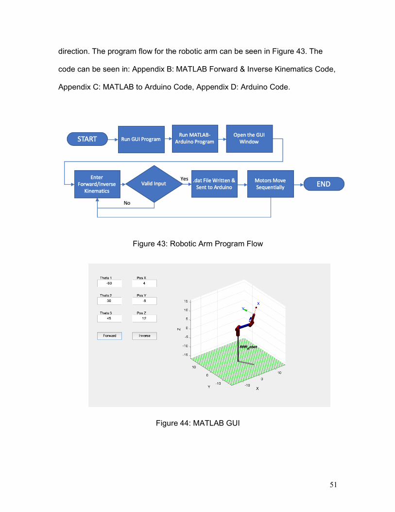
6.3. Programming Formulation

Using the robotic toolbox, the robotic arm in this project was programmed in

MATLAB to have a Graphical User Interface (GUI), through which a user can

input either the forward or inverse kinematics. When inputting the angles in

degrees, it solves for the X, Y and Z coordinates; this is the forward kinematic

solution. When inputting the location of the end effector in terms of X, Y and Z

coordinates it solves for the optimal solution for the angles between the links, this

is the inverse kinematic solution. This code then generates the number of steps

and direction required by each motor and saves it to a .dat file. In a second

MATLAB program, the data from the .dat file is extracted and put into a string to

be sent to Arduino to read. Once the command is sent; Arduino reads the string

and moves the motors sequentially the appropriate number of steps in the correct

51

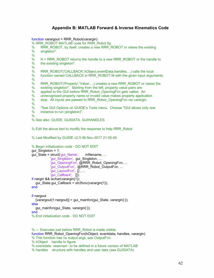
direction. The program flow for the robotic arm can be seen in Figure 43. The

code can be seen in: Appendix B: MATLAB Forward & Inverse Kinematics Code,

Appendix C: MATLAB to Arduino Code, Appendix D: Arduino Code.

Figure 43: Robotic Arm Program Flow

Figure 44: MATLAB GUI

52

Due to link 1 being 6 inches long and link 2 being 4 inches long there are some

limitations to what can be entered for the inverse kinematics. The following are

the range of maximum values, the workspace, should the other two variables be

zero.

X Limit: -9:9

Y Limit: -9:9

Z Limit: -7:12

The robotic toolbox was used because it allowed for easier visualization, allows

for easier extension to more DOF and it solves for the inverse kinematics, which

otherwise would have been complex to code, as all possible solutions need to be

evaluated and the best one needs to be selected. The toolbox computes the

inverse kinematics by optimization without joint limits solution iteratively,

implementing a Levenberg-Marquadt variable step size solver. The tolerance is

computed on the norm of the error between the current and the desired tool

pose. This norm is computed from distances and angles without any kind of

weighting. This approach allows a solution to be obtained at a singularity, but the

joint angles within the null space are arbitrarily assigned. [21]

53

6.4. Key Questions

Some key questions and concepts to consider during the programming phase

are:

- What are the advantages and disadvantages of using a robotics

library?

- How can the program and data flow be more efficient?

- How can the workspace be enforced?

- Should the motors move sequentially or simultaneously?

- How can the code be validated to prove the movement results in the

correct location of the end effector?

- What kind of safety checks should be included in the code?

- Are there failsafe mechanisms in the code?

- What are the failure modes of the robotic arm due to programming?

54

7.0 Discussion

7.1. Summary

This educational platform was developed with the specific purpose of integrating

different engineering disciplines for students to create a technology enabled

product that represents modern technology and the practical applications. It was

designed with the intention of motivating and exciting students to adapt, evolve

and develop their engineering knowledge, as well as bridge the gap between

theory and application, while also honing their cross-functional engineering

capabilities.

The educational platform developed and discussed in this thesis serves as

design and construction procedures for a robotic manipulator. It outlines the

suggested steps, key decisions, and the design and construction of one possible

functional robotic arm. The educational platform proposed in this thesis is broad

which allows it to be “extensible” to cover areas beyond those discussed.

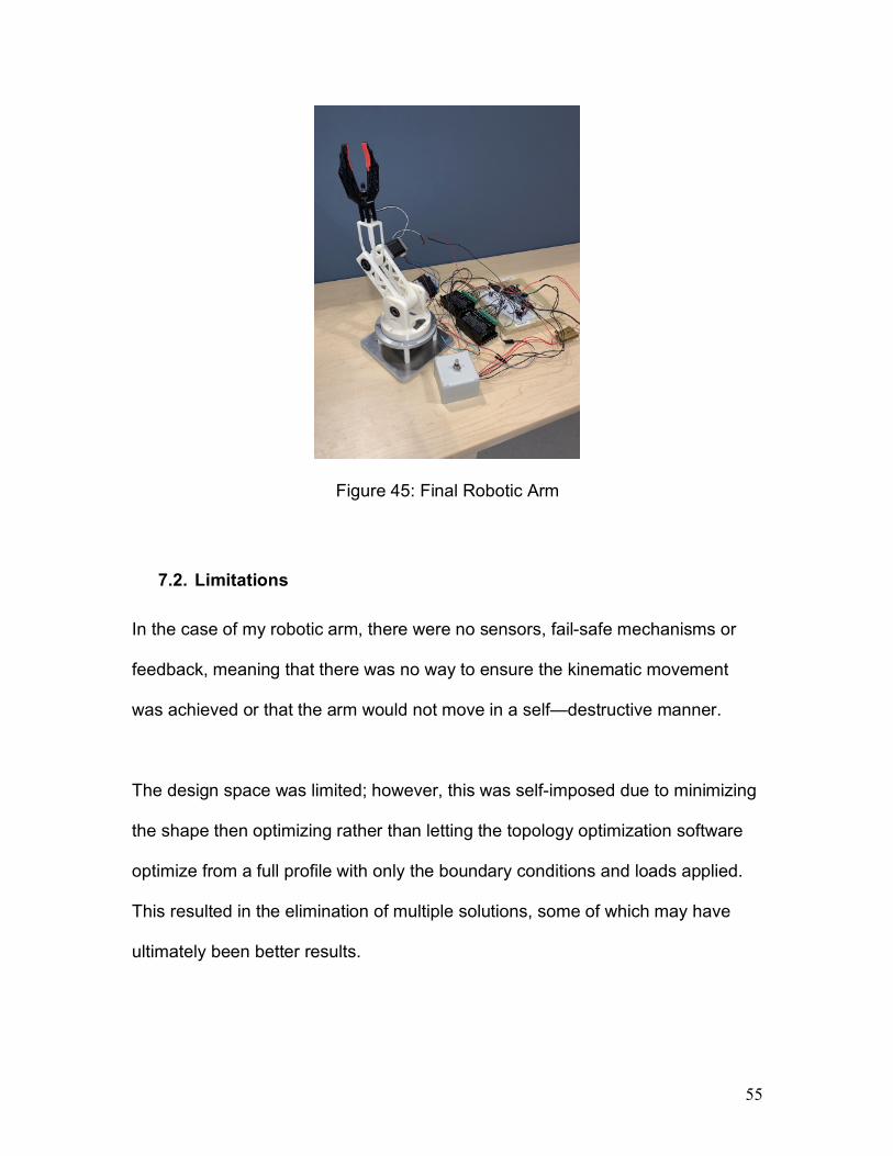
As seen in Figure 45, the robotic arm discussed in this thesis, was developed

and created. All the simulation was completed with carbon fiber as the material,

however the robotic arm was printed with abs plastic using a Stratasys F170

printer for demonstration purposes.

55

Figure 45: Final Robotic Arm

7.2. Limitations

In the case of my robotic arm, there were no sensors, fail-safe mechanisms or

feedback, meaning that there was no way to ensure the kinematic movement

was achieved or that the arm would not move in a self—destructive manner.

The design space was limited; however, this was self-imposed due to minimizing

the shape then optimizing rather than letting the topology optimization software

optimize from a full profile with only the boundary conditions and loads applied.

This resulted in the elimination of multiple solutions, some of which may have

ultimately been better results.

56

7.3. Implementation

The development process of the robotic arm offers insightful lessons valuable for

engineering students including:

- How to apply the theory of an array of different engineering topics

- Not to put unnecessary constraints, as it will inhibit the design, make it

less efficient and a challenge to design around

- Exposure to the design and development process and problem solving

- Most importantly, the concept that every decision has a ripple effect

and that students should employ a holistic approach

For engineering students to benefit from this educational platform the next step is

to implement this project into a course. The vision for this educational platform is

for it to be an entire course, such as “Toy Design”.

Design this course to be fun and engaging. This will particularly appeal to

students who learn more effectively through “hands-on” application-based

projects versus through derivation.

It would be beneficial for students to work in two-person groups. This will spark

collaboration and promote teamwork. Small groups will hopefully prevent any one

student from completing a disproportionate amount of the work.

57

Provide structure for student success by creating milestones. This allows

students the flexibility to work independently, simulating what an engineer would

face in industry.

Encourage students to be innovative both in their creativity and their approach to

applying theoretical concepts. This thesis outlines design and construction

procedures therefore, students should aim to add or improve some aspect of the

project such as, the robotic arm completing a specific task or increasing DOF.

This educational platform is modular, allowing it to be built upon or modified to

include additional or different courses.

7.4. Future Development of Project

Students should aim to improve the robotic arm by eliminating the existing

limitations. Utilizing sensors, fail-safe mechanisms and feedback, will ensure the

kinematic movement is achieved and that the arm will not move in a self—

destructive manner. The program and data flow of the robotic arm should be

enhanced to make it more efficient. The design space should be enlarged from

the beginning to take full advantage of the topology optimization software in order

to yield the best results.

As students develop the robotic arm and integrate different fields of engineering,

they can challenge themselves by adding on different components. For example:

58

they can increase the DOF or use a Kinect Camera to have the robotic arm track

and mimic a person’s movement. The project can be developed and adapted in a

myriad of ways with a student’s creativity, determination and time.

59

8.0 References [1] Taborda, Elkin, Senthil K. Chandrasegaran, and Karthik Ramani. "Me 444:

Redesigning a toy design course." International Symposium Tools and Methods of Competitive Engineering (TMCE), Karlsruhe, Germany, May. 2012.

[2] “Homepage.” PLTW, https://www.pltw.org. [3] Lynxmotion AL5D PLTW Robotic Arm Kit.

https://www.robotshop.com/en/lynxmotion-al5d-pltw-robotic-arm-kit.html [4] Lynxmotion AL5D PLTW Robotic Arm - Assembled.

https://www.robotshop.com/en/lynxmotion-al5d-pltw-robotic-arm-assembled.html.

[5] Chapter 4. Basic Kinematics of Constrained Rigid Bodies. https://www.cs.cmu.edu/~rapidproto/mechanisms/chpt4.html#top.

[6] Moeini, Masoud. Dynamics Analysis for a 3-RPS1 Parallel Manipulator Wearable Thimble.

[7] Coordinate Transformations. http://what-when-how.com/wp-content/uploads/2012/06/tmpc00939.png.

[8] Foley, James D., et al. Computer graphics: principles and practice. Vol. 12110. Addison-Wesley Professional, 1996.

[9] “KINEMATICS ANALYSIS OF ROBOTS (Part 3)” SlidePlayer, slideplayer.com/slide/6636263/.

[10] Denavit, Jacques. "A kinematic notation for low pair mechanisms based on matrices." ASME J. Appl. Mech. 22 (1955): 215-221.

[11] Shiriaev, Anton. Kinematics: Forward and Inverse Kinematics. http://www8.tfe.umu.se/courses/elektro/RobotControl/Lecture04_5EL158.pdf.

[12] Spong, Mark W., and Mathukumalli Vidyasagar. Robot dynamics and control. John Wiley & Sons, 2008.

[13] Gosselin, Clement, and Jorge Angeles. "Singularity analysis of closed-loop kinematic chains." IEEE transactions on robotics and automation 6.3 (1990): 281-290.

[14] 3D Printer Continuous Carbon Fiber Filament Material | Markforged. https://markforged.com/materials/carbon-fiber/.

[15] Markforged Composites Datasheet. https://static.markforged.com/markforged_composites_datasheet.pdf.

[16] Waterman, Pamela. “Simulate to Shed Weight Sooner.” Digital Engineering 247, 1 Jan. 2016, www.digitalengineering247.com/article/wp-content/uploads/2015/12/VRDgtam_5400.jpg.

[17] AMCI : Advanced Micro Controls Inc :: Stepper vs Servo. https://www.amci.com/industrial-automation-resources/plc-automation-tutorials/stepper-vs-servo/.

[18] Amazon.com: Makeblock Robot Gripper with Four Standard M4 Thread Holes Easy Assembly: Industrial & Scientific. https://www.amazon.com/dp/B00WG3KTL4/ref=asc_df_B00WG3KTL45418483/?tag=hyprod--310149419221.

60

[19] “Ohms Law Tutorial and Power in Electrical Circuits.” Basic Electronics Tutorials, 11 Aug. 2013, https://www.electronics-tutorials.ws/dccircuits/dcp_2.html.

[20] Rosen, David W., et al. "Design for Additive Manufacturing: A Paradigm Shift in Design, Fabrication, and Qualification." Journal of Mechanical Design 137.11 (2015): 110301.

[21] Corke, Peter. Robotics, vision and control: fundamental algorithms in MATLAB® second, completely revised. Vol. 118. Springer, 2017.

61

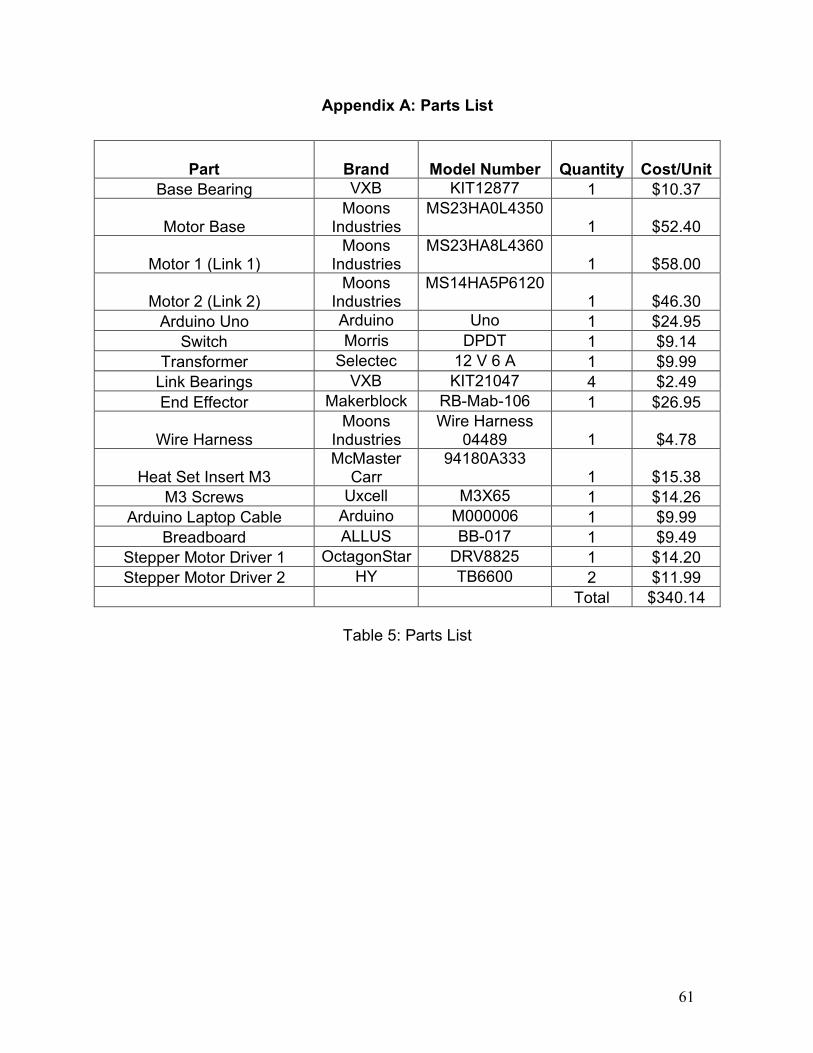
Appendix A: Parts List

Part

Brand

Model Number Quantity Cost/Unit Base Bearing VXB KIT12877 1 $10.37

Motor Base Moons

Industries MS23HA0L4350

1 $52.40

Motor 1 (Link 1) Moons

Industries MS23HA8L4360

1 $58.00

Motor 2 (Link 2) Moons

Industries MS14HA5P6120

1 $46.30 Arduino Uno Arduino Uno 1 $24.95

Switch Morris DPDT 1 $9.14 Transformer Selectec 12 V 6 A 1 $9.99

Link Bearings VXB KIT21047 4 $2.49 End Effector Makerblock RB-Mab-106 1 $26.95

Wire Harness Moons

Industries Wire Harness

04489 1 $4.78

Heat Set Insert M3 McMaster

Carr 94180A333

1 $15.38 M3 Screws Uxcell M3X65 1 $14.26

Arduino Laptop Cable Arduino M000006 1 $9.99 Breadboard ALLUS BB-017 1 $9.49

Stepper Motor Driver 1 OctagonStar DRV8825 1 $14.20 Stepper Motor Driver 2 HY TB6600 2 $11.99

Total $340.14

Table 5: Parts List

62

Appendix B: MATLAB Forward & Inverse Kinematics Code function varargout = RRR_Robot(varargin) % RRR_ROBOT MATLAB code for RRR_Robot.fig % RRR_ROBOT, by itself, creates a new RRR_ROBOT or raises the existing % singleton*. % % H = RRR_ROBOT returns the handle to a new RRR_ROBOT or the handle to % the existing singleton*. % % RRR_ROBOT('CALLBACK',hObject,eventData,handles,...) calls the local % function named CALLBACK in RRR_ROBOT.M with the given input arguments. % % RRR_ROBOT('Property','Value',...) creates a new RRR_ROBOT or raises the % existing singleton*. Starting from the left, property value pairs are % applied to the GUI before RRR_Robot_OpeningFcn gets called. An % unrecognized property name or invalid value makes property application % stop. All inputs are passed to RRR_Robot_OpeningFcn via varargin. % % *See GUI Options on GUIDE's Tools menu. Choose "GUI allows only one % instance to run (singleton)". % % See also: GUIDE, GUIDATA, GUIHANDLES % Edit the above text to modify the response to help RRR_Robot % Last Modified by GUIDE v2.5 06-Nov-2017 21:50:49 % Begin initialization code - DO NOT EDIT gui_Singleton = 1; gui_State = struct('gui_Name', mfilename, ... 'gui_Singleton', gui_Singleton, ... 'gui_OpeningFcn', @RRR_Robot_OpeningFcn, ... 'gui_OutputFcn', @RRR_Robot_OutputFcn, ... 'gui_LayoutFcn', [] , ... 'gui_Callback', []); if nargin && ischar(varargin{1}) gui_State.gui_Callback = str2func(varargin{1}); end if nargout [varargout{1:nargout}] = gui_mainfcn(gui_State, varargin{:}); else gui_mainfcn(gui_State, varargin{:}); end % End initialization code - DO NOT EDIT % --- Executes just before RRR_Robot is made visible. function RRR_Robot_OpeningFcn(hObject, eventdata, handles, varargin) % This function has no output args, see OutputFcn. % hObject handle to figure % eventdata reserved - to be defined in a future version of MATLAB % handles structure with handles and user data (see GUIDATA)

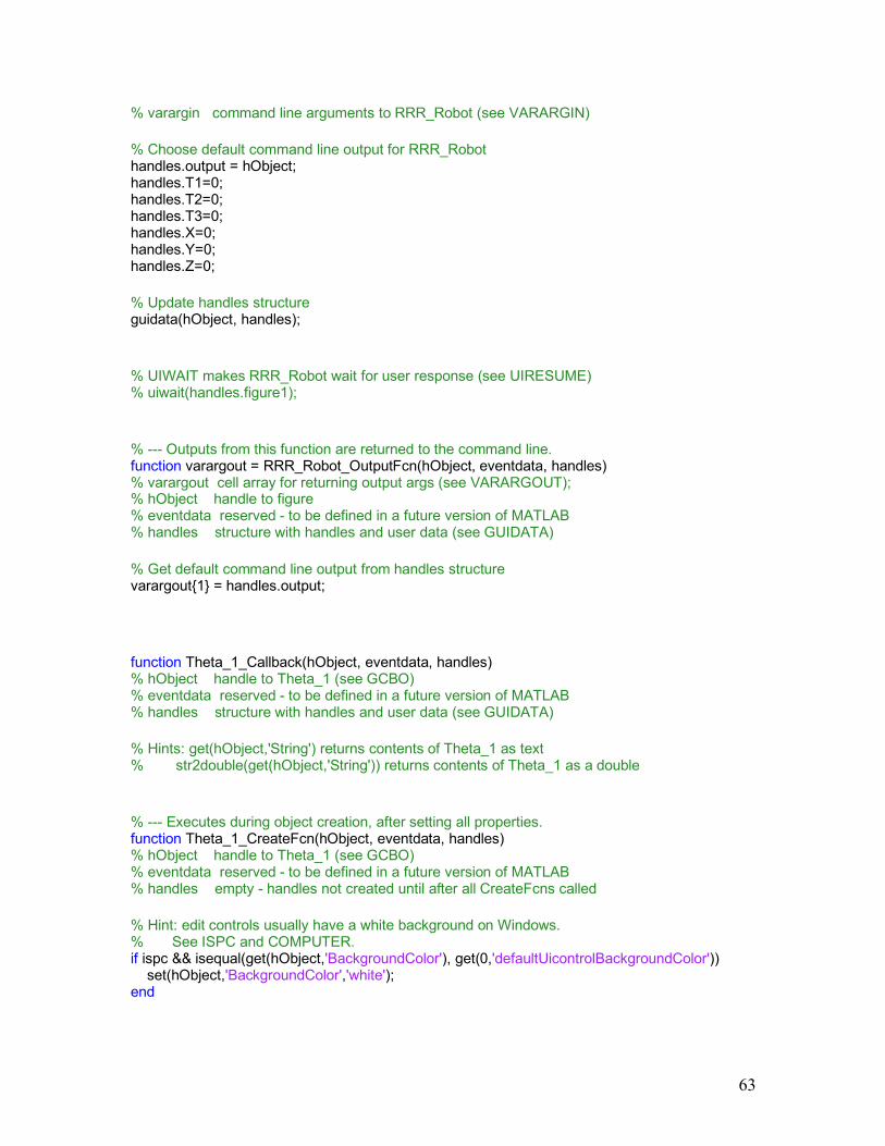
63

% varargin command line arguments to RRR_Robot (see VARARGIN) % Choose default command line output for RRR_Robot handles.output = hObject; handles.T1=0; handles.T2=0; handles.T3=0; handles.X=0; handles.Y=0; handles.Z=0; % Update handles structure guidata(hObject, handles); % UIWAIT makes RRR_Robot wait for user response (see UIRESUME) % uiwait(handles.figure1); % --- Outputs from this function are returned to the command line. function varargout = RRR_Robot_OutputFcn(hObject, eventdata, handles) % varargout cell array for returning output args (see VARARGOUT); % hObject handle to figure % eventdata reserved - to be defined in a future version of MATLAB % handles structure with handles and user data (see GUIDATA) % Get default command line output from handles structure varargout{1} = handles.output; function Theta_1_Callback(hObject, eventdata, handles) % hObject handle to Theta_1 (see GCBO) % eventdata reserved - to be defined in a future version of MATLAB % handles structure with handles and user data (see GUIDATA) % Hints: get(hObject,'String') returns contents of Theta_1 as text % str2double(get(hObject,'String')) returns contents of Theta_1 as a double % --- Executes during object creation, after setting all properties. function Theta_1_CreateFcn(hObject, eventdata, handles) % hObject handle to Theta_1 (see GCBO) % eventdata reserved - to be defined in a future version of MATLAB % handles empty - handles not created until after all CreateFcns called % Hint: edit controls usually have a white background on Windows. % See ISPC and COMPUTER. if ispc && isequal(get(hObject,'BackgroundColor'), get(0,'defaultUicontrolBackgroundColor')) set(hObject,'BackgroundColor','white'); end

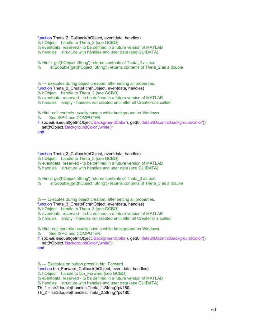
64

function Theta_2_Callback(hObject, eventdata, handles) % hObject handle to Theta_2 (see GCBO) % eventdata reserved - to be defined in a future version of MATLAB % handles structure with handles and user data (see GUIDATA) % Hints: get(hObject,'String') returns contents of Theta_2 as text % str2double(get(hObject,'String')) returns contents of Theta_2 as a double % --- Executes during object creation, after setting all properties. function Theta_2_CreateFcn(hObject, eventdata, handles) % hObject handle to Theta_2 (see GCBO) % eventdata reserved - to be defined in a future version of MATLAB % handles empty - handles not created until after all CreateFcns called % Hint: edit controls usually have a white background on Windows. % See ISPC and COMPUTER. if ispc && isequal(get(hObject,'BackgroundColor'), get(0,'defaultUicontrolBackgroundColor')) set(hObject,'BackgroundColor','white'); end function Theta_3_Callback(hObject, eventdata, handles) % hObject handle to Theta_3 (see GCBO) % eventdata reserved - to be defined in a future version of MATLAB % handles structure with handles and user data (see GUIDATA) % Hints: get(hObject,'String') returns contents of Theta_3 as text % str2double(get(hObject,'String')) returns contents of Theta_3 as a double % --- Executes during object creation, after setting all properties. function Theta_3_CreateFcn(hObject, eventdata, handles) % hObject handle to Theta_3 (see GCBO) % eventdata reserved - to be defined in a future version of MATLAB % handles empty - handles not created until after all CreateFcns called % Hint: edit controls usually have a white background on Windows. % See ISPC and COMPUTER. if ispc && isequal(get(hObject,'BackgroundColor'), get(0,'defaultUicontrolBackgroundColor')) set(hObject,'BackgroundColor','white'); end % --- Executes on button press in btn_Forward. function btn_Forward_Callback(hObject, eventdata, handles) % hObject handle to btn_Forward (see GCBO) % eventdata reserved - to be defined in a future version of MATLAB % handles structure with handles and user data (see GUIDATA) Th_1 = str2double(handles.Theta_1.String)*pi/180; Th_2 = str2double(handles.Theta_2.String)*pi/180;

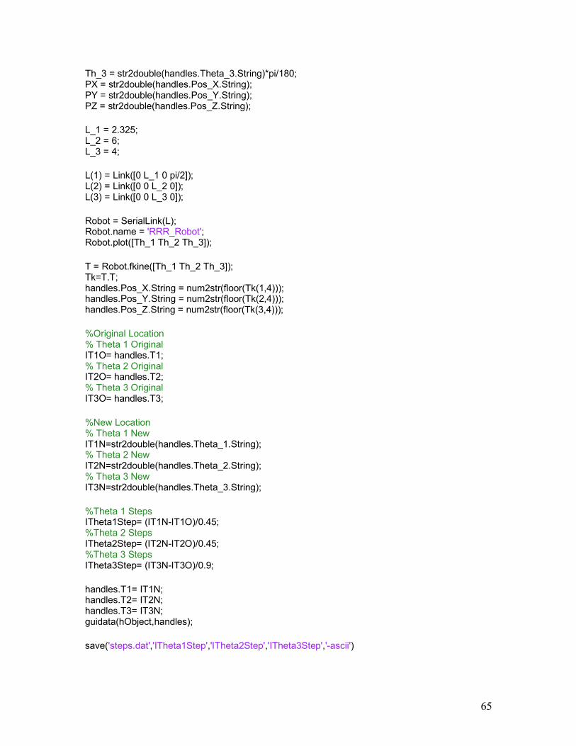
65

Th_3 = str2double(handles.Theta_3.String)*pi/180; PX = str2double(handles.Pos_X.String); PY = str2double(handles.Pos_Y.String); PZ = str2double(handles.Pos_Z.String); L_1 = 2.325; L_2 = 6; L_3 = 4; L(1) = Link([0 L_1 0 pi/2]); L(2) = Link([0 0 L_2 0]); L(3) = Link([0 0 L_3 0]); Robot = SerialLink(L); Robot.name = 'RRR_Robot'; Robot.plot([Th_1 Th_2 Th_3]); T = Robot.fkine([Th_1 Th_2 Th_3]); Tk=T.T; handles.Pos_X.String = num2str(floor(Tk(1,4))); handles.Pos_Y.String = num2str(floor(Tk(2,4))); handles.Pos_Z.String = num2str(floor(Tk(3,4))); %Original Location % Theta 1 Original IT1O= handles.T1; % Theta 2 Original IT2O= handles.T2; % Theta 3 Original IT3O= handles.T3; %New Location % Theta 1 New IT1N=str2double(handles.Theta_1.String); % Theta 2 New IT2N=str2double(handles.Theta_2.String); % Theta 3 New IT3N=str2double(handles.Theta_3.String); %Theta 1 Steps ITheta1Step= (IT1N-IT1O)/0.45; %Theta 2 Steps ITheta2Step= (IT2N-IT2O)/0.45; %Theta 3 Steps ITheta3Step= (IT3N-IT3O)/0.9; handles.T1= IT1N; handles.T2= IT2N; handles.T3= IT3N; guidata(hObject,handles); save('steps.dat','ITheta1Step','ITheta2Step','ITheta3Step','-ascii')

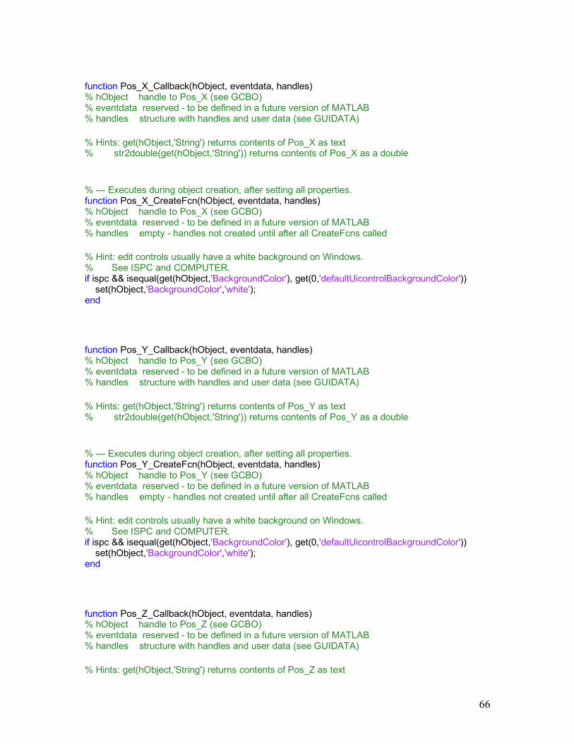
66

function Pos_X_Callback(hObject, eventdata, handles) % hObject handle to Pos_X (see GCBO) % eventdata reserved - to be defined in a future version of MATLAB % handles structure with handles and user data (see GUIDATA) % Hints: get(hObject,'String') returns contents of Pos_X as text % str2double(get(hObject,'String')) returns contents of Pos_X as a double % --- Executes during object creation, after setting all properties. function Pos_X_CreateFcn(hObject, eventdata, handles) % hObject handle to Pos_X (see GCBO) % eventdata reserved - to be defined in a future version of MATLAB % handles empty - handles not created until after all CreateFcns called % Hint: edit controls usually have a white background on Windows. % See ISPC and COMPUTER. if ispc && isequal(get(hObject,'BackgroundColor'), get(0,'defaultUicontrolBackgroundColor')) set(hObject,'BackgroundColor','white'); end function Pos_Y_Callback(hObject, eventdata, handles) % hObject handle to Pos_Y (see GCBO) % eventdata reserved - to be defined in a future version of MATLAB % handles structure with handles and user data (see GUIDATA) % Hints: get(hObject,'String') returns contents of Pos_Y as text % str2double(get(hObject,'String')) returns contents of Pos_Y as a double % --- Executes during object creation, after setting all properties. function Pos_Y_CreateFcn(hObject, eventdata, handles) % hObject handle to Pos_Y (see GCBO) % eventdata reserved - to be defined in a future version of MATLAB % handles empty - handles not created until after all CreateFcns called % Hint: edit controls usually have a white background on Windows. % See ISPC and COMPUTER. if ispc && isequal(get(hObject,'BackgroundColor'), get(0,'defaultUicontrolBackgroundColor')) set(hObject,'BackgroundColor','white'); end function Pos_Z_Callback(hObject, eventdata, handles) % hObject handle to Pos_Z (see GCBO) % eventdata reserved - to be defined in a future version of MATLAB % handles structure with handles and user data (see GUIDATA) % Hints: get(hObject,'String') returns contents of Pos_Z as text

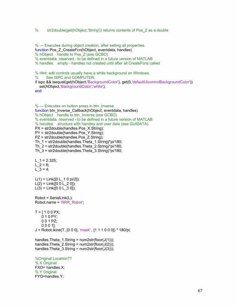
67

% str2double(get(hObject,'String')) returns contents of Pos_Z as a double % --- Executes during object creation, after setting all properties. function Pos_Z_CreateFcn(hObject, eventdata, handles) % hObject handle to Pos_Z (see GCBO) % eventdata reserved - to be defined in a future version of MATLAB % handles empty - handles not created until after all CreateFcns called % Hint: edit controls usually have a white background on Windows. % See ISPC and COMPUTER. if ispc && isequal(get(hObject,'BackgroundColor'), get(0,'defaultUicontrolBackgroundColor')) set(hObject,'BackgroundColor','white'); end % --- Executes on button press in btn_Inverse. function btn_Inverse_Callback(hObject, eventdata, handles) % hObject handle to btn_Inverse (see GCBO) % eventdata reserved - to be defined in a future version of MATLAB % handles structure with handles and user data (see GUIDATA) PX = str2double(handles.Pos_X.String); PY = str2double(handles.Pos_Y.String); PZ = str2double(handles.Pos_Z.String); Th_1 = str2double(handles.Theta_1.String)*pi/180; Th_2 = str2double(handles.Theta_2.String)*pi/180; Th_3 = str2double(handles.Theta_3.String)*pi/180; L_1 = 2.325; L_2 = 6; L_3 = 4; L(1) = Link([0 L_1 0 pi/2]); L(2) = Link([0 0 L_2 0]); L(3) = Link([0 0 L_3 0]); Robot = SerialLink(L); Robot.name = 'RRR_Robot'; T = [ 1 0 0 PX; 0 1 0 PY; 0 0 1 PZ; 0 0 0 1]; J = Robot.ikine(T, [0 0 0], 'mask' , [1 1 1 0 0 0]) * 180/pi; handles.Theta_1.String = num2str(floor(J(1))); handles.Theta_2.String = num2str(floor(J(2))); handles.Theta_3.String = num2str(floor(J(3))); %Original Location?? % X Original FXO= handles.X; % Y Original FYO=handles.Y;

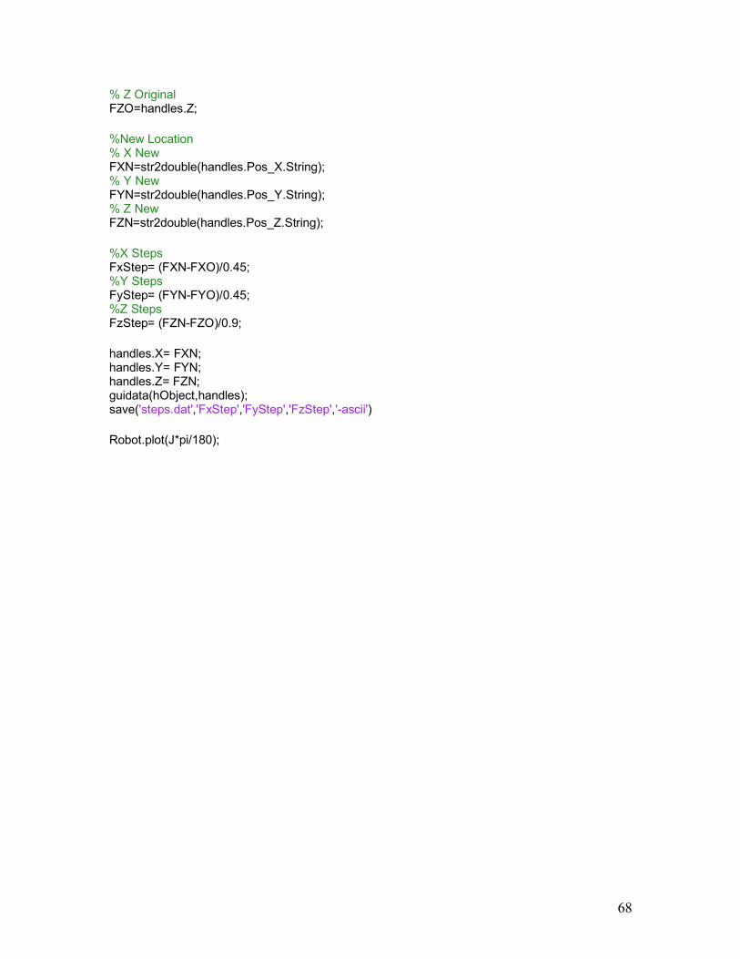
68

% Z Original FZO=handles.Z; %New Location % X New FXN=str2double(handles.Pos_X.String); % Y New FYN=str2double(handles.Pos_Y.String); % Z New FZN=str2double(handles.Pos_Z.String); %X Steps FxStep= (FXN-FXO)/0.45; %Y Steps FyStep= (FYN-FYO)/0.45; %Z Steps FzStep= (FZN-FZO)/0.9; handles.X= FXN; handles.Y= FYN; handles.Z= FZN; guidata(hObject,handles); save('steps.dat','FxStep','FyStep','FzStep','-ascii') Robot.plot(J*pi/180);

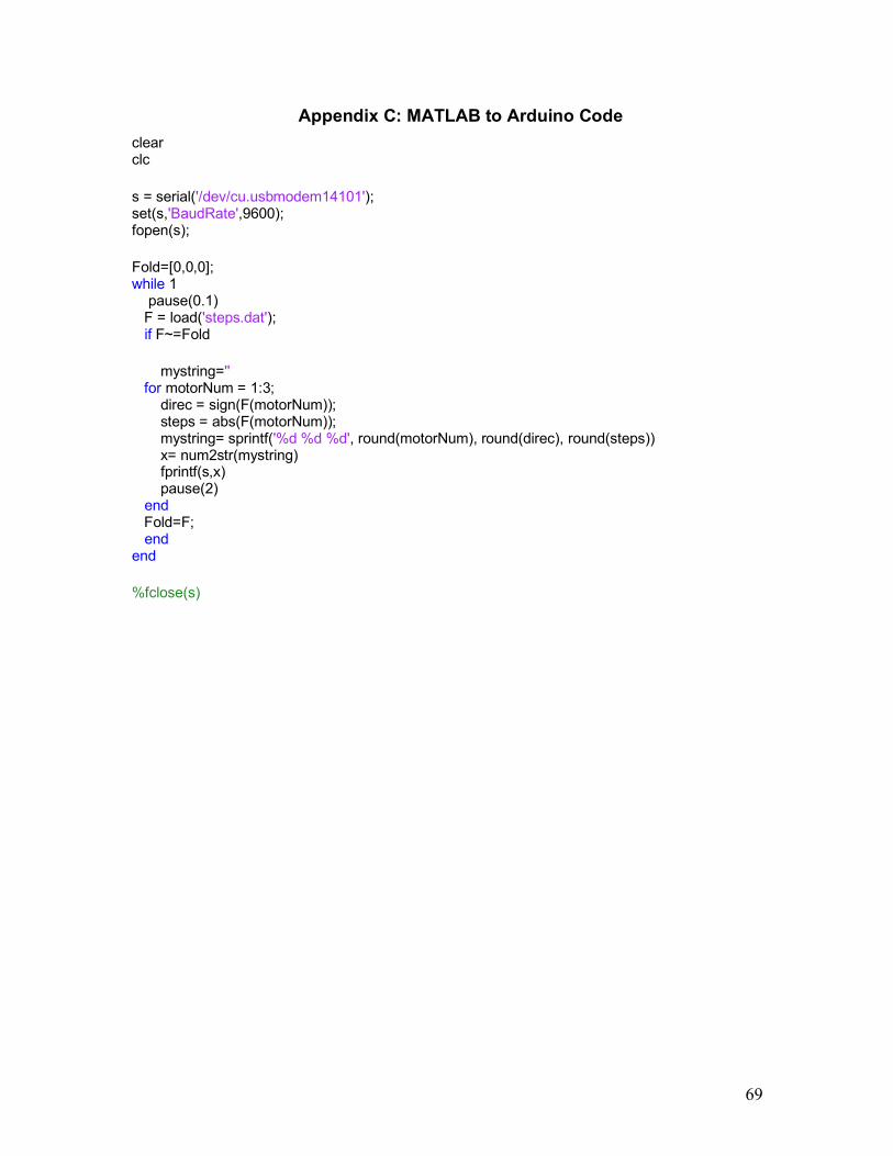
69

Appendix C: MATLAB to Arduino Code clear clc s = serial('/dev/cu.usbmodem14101'); set(s,'BaudRate',9600); fopen(s); Fold=[0,0,0]; while 1 pause(0.1) F = load('steps.dat'); if F~=Fold mystring='' for motorNum = 1:3; direc = sign(F(motorNum)); steps = abs(F(motorNum)); mystring= sprintf('%d %d %d', round(motorNum), round(direc), round(steps)) x= num2str(mystring) fprintf(s,x) pause(2) end Fold=F; end end %fclose(s)

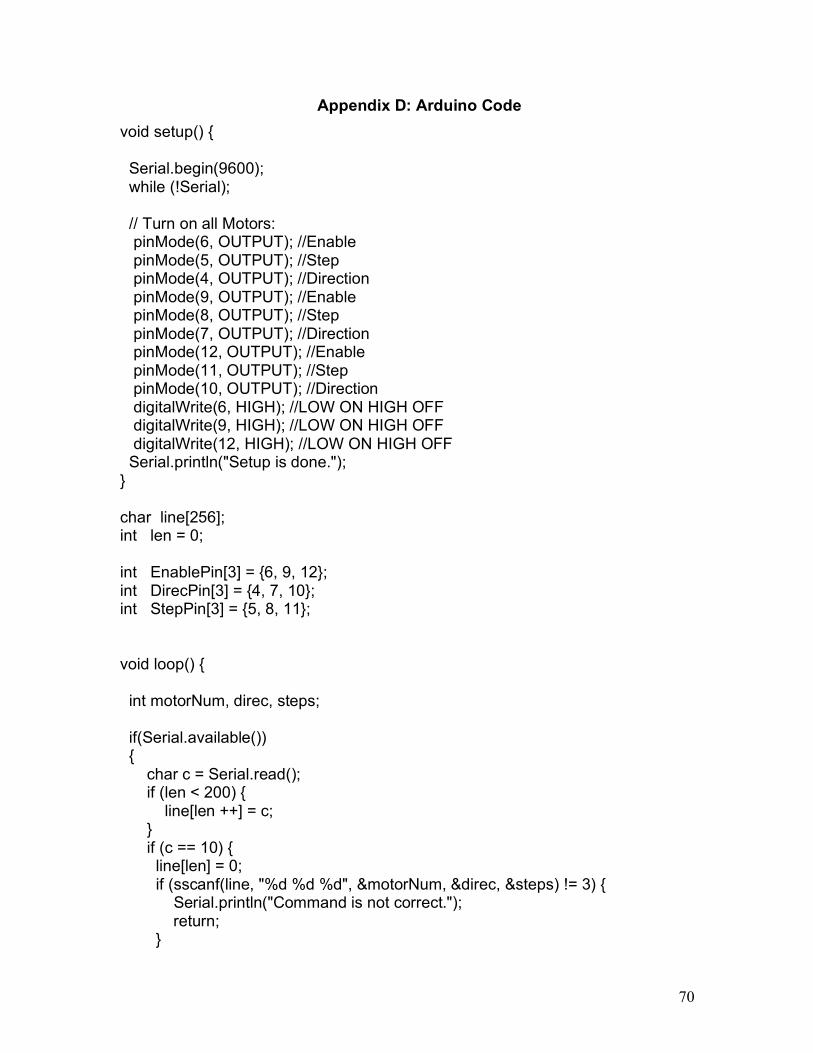
70

Appendix D: Arduino Code void setup() { Serial.begin(9600); while (!Serial); // Turn on all Motors: pinMode(6, OUTPUT); //Enable pinMode(5, OUTPUT); //Step pinMode(4, OUTPUT); //Direction pinMode(9, OUTPUT); //Enable pinMode(8, OUTPUT); //Step pinMode(7, OUTPUT); //Direction pinMode(12, OUTPUT); //Enable pinMode(11, OUTPUT); //Step pinMode(10, OUTPUT); //Direction digitalWrite(6, HIGH); //LOW ON HIGH OFF digitalWrite(9, HIGH); //LOW ON HIGH OFF digitalWrite(12, HIGH); //LOW ON HIGH OFF Serial.println("Setup is done."); } char line[256]; int len = 0; int EnablePin[3] = {6, 9, 12}; int DirecPin[3] = {4, 7, 10}; int StepPin[3] = {5, 8, 11}; void loop() { int motorNum, direc, steps; if(Serial.available()) { char c = Serial.read(); if (len < 200) { line[len ++] = c; } if (c == 10) { line[len] = 0; if (sscanf(line, "%d %d %d", &motorNum, &direc, &steps) != 3) { Serial.println("Command is not correct."); return; }

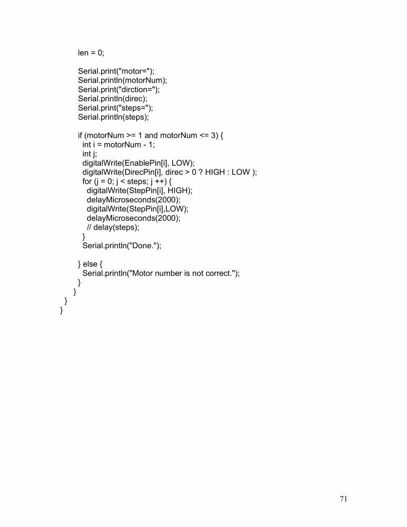
71

len = 0; Serial.print("motor="); Serial.println(motorNum); Serial.print("dirction="); Serial.println(direc); Serial.print("steps="); Serial.println(steps); if (motorNum >= 1 and motorNum <= 3) { int i = motorNum - 1; int j; digitalWrite(EnablePin[i], LOW); digitalWrite(DirecPin[i], direc > 0 ? HIGH : LOW ); for (j = 0; j < steps; j ++) { digitalWrite(StepPin[i], HIGH); delayMicroseconds(2000); digitalWrite(StepPin[i],LOW); delayMicroseconds(2000); // delay(steps); } Serial.println("Done."); } else { Serial.println("Motor number is not correct."); } } } }