3d-models of railway track for dynamic analysis467217/fulltext01.pdf · discrete support model,...
TRANSCRIPT

3D-models of Railway Track
for Dynamic Analysis
Master Degree Project
Huan Feng
Division of Highway and Railway Engineering
Department of Transport Science
School of Architecture and the Built Environment
Royal Institute of Technology
SE-100 44 Stockholm
TRITA-VBT 11:16
ISSN 1650-867X
ISRN KTH/VBT-11/16-SE
Stockholm 2011


i
Preface
This master thesis was carried out at the Division of Highway and Railway Engineering, at
the Royal Institute of Technology (KTH) in Stockholm. The work was conducted under the
supervision of Assistant Prof. Elias Kassa to whom I want to thank for valuable guidance and
advice and whom also was the examiner. I also want to thank Tekn. Dr. Andreas Andersson
and PhD Candidate John Leander for the help provided and interesting discussions.
Stockholm, November 2011
Huan Feng


iii
Abstract
In recent decades, railway transport infrastructures have been regaining their importance due
to their efficiency and environmentally friendly technologies. This has led to increasing train
speeds, higher axle loads and more frequent train usage. These improved service provisions
have however brought new challenges to traditional railway track engineering, especially to
track geotechnical dynamics. These challenges demanded for a better understanding of the
track dynamics. Due to the large cost and available load conditions limitation, experimental
investigation is not always the best choice for the dynamic effect study of railway track
structure. Comparatively speaking, an accurate mathematical modeling and numerical
solution of the dynamic interaction of the track structural components reveals distinct
advantage for understanding the response behavior of the track structure.
The purpose of this thesis is to study the influence of design parameters on dynamic response
of the railway track structure by implementing Finite Element Method (FEM). According to
the complexity, different railway track systems have been simulated, including: Beam on
discrete support model, Discretely support track including ballast mass model and Rail on
sleeper on continuum model. The rail and sleeper have been modeled by Euler-Bernoulli
beam element. Spring and dashpot has been used for the simulation of railpads and the
connection between the sleeper and ballast ground. Track components have been studied
separately and comparisons have been made between different models.
The finite element analysis is divided into three categories: eigenvalue analysis, dynamic
analysis and general static analysis. The eigenfrequencies and corresponding vibration modes
were extracted from all the models. The main part of the finite element modeling involves the
steady-state dynamic analysis, in which receptance functions were obtained and used as the
criterion for evaluating the dynamic properties of track components. Dynamic explicit
analysis has been used for the simulation of a moving load, and the train speed effect has been
studied. The displacement of the trackbed has been evaluated and compared to the
measurement taken in Sweden in the static analysis.
Keywords: track dynamics, railway track modelling, finite element analysis, receptance


v
Abstrakt
Under de senaste decennierna har järnvägsnätet återvunnit sin betydelse genom sin höga
effektivitet och miljövänliga teknik. Under denna senare period har både tåghastigheten samt
axeltrycken höjts och därigenom skapat utrymme för en högre utnyttjandegrad av
järnvägsnätet, med tätare avgångar. Dessa förbättringar har dock medfört nya utmaningar som
måste beaktas och implementeras inom den traditionella järnvägstekniken, inte minst
beaktandet av dynamiska effekter inom geoteknik. På grund av den höga kostnaden, samt
begränsning av aktuella lastsituationer, är undersökningar i fällt inte alltid det bästa valet vid
undersökning av dynamiska effekter. Jämförelsevis kan en noggrann matematisk modell, med
dess numeriska lösning av interaktionsproblemet, underlätta vid beskrivningen av samspelet
för den sammansatta konstruktionen och dess beteende.
Syftet med denna uppsats är att studera inverkan av olika parametrar kopplade till den
dynamiska responsen av en järnvägskonstruktion genom att implementera finita
elementmetoden (FEM). På grund av komplexitet, vilket karakteriserar problemet, har olika
modeller undersökts och simulerats. Inkluderade modeller är: Balk på diskreta stöd, Räls
modellerad på diskreta stöd med medverkande massa från ballast samt räls och sliper
modellerad i samverkan men en kontinuummekanisk modell. Rälen och slipern har
modellerats som ett Euler-Bernulli balkelement. Den fysikaliska beskrivningen av mellan räl
och sliper samt sliper ballast är modellerad som massa-fjäder-dämpar-system. De olika
ingående komponenterna har studerats separat och jämförelser har gjorts mellan de olika
modellerna.
Finita elementanalysen är uppdelad i följande tre delar: egenvärdesanalys, dynamisk analys
samt statisk analys. Egenfrekvenserna och dess tillhörande svängningsmoder är presenterade
för samtliga modeller. Merdelen av finita elementmodelleringen beskriver den dynamiska
jämvikten, där erhölls och användes som kriterium för utvärdering av de olika dynamiskt
länkade parametrarna. Vid simulering av rörlig last och dess hastighetsvariation har används.
Förskjutningen av järnvägskonstruktionen har utvärderats och jämförts med mätningar
utförda i Sverige för motsvarande konstruktion under statisk analys.
Nyckelord: spår dynamisk, järnvägs bana, finita element analys, receptance


vii
Contents
Preface i
Abstract iii
Abstrakt v
1 Introduction 1
1.1 Introduction................................................................................................................ 1
1.2 Properties of the Railway track ................................................................................... 1
1.3 Aims of the Study ........................................................................................................ 3
1.4 Structure of the Thesis ................................................................................................. 4
2 Literature Reviews 7
2.1 Dynamic properties of track components ................................................................... 5
2.1.1 The rail ........................................................................................................... 5
2.1.2 The railpads and fastening .............................................................................. 8
2.1.3 The sleepers .................................................................................................... 9
2.1.4 The ballast, subballast and subgrade .............................................................. 9
2.2 Dynamic Properties of the Track .............................................................................. 11
2.2.1 Receptance ................................................................................................... 11
2.2.2 Resonance .................................................................................................... 12
2.3 Forces exerted on ballast .......................................................................................... 14
2.4 Train speed effect ..................................................................................................... 15
2.4 Mathematical model ................................................................................................. 17
2.5.1 Beam on elastic foundation (BOEF) model ................................................. 17
2.5.2 Beam (rail) on discrete supports .................................................................. 18
2.5.3 Discretely supported rail including ballast mass ......................................... 19
2.5.4 Tensionless BOEF model according to Kjell Arne Skoglund ..................... 20
2.5.5 Pasternak foundation .................................................................................... 21

viii
2.5.6 Other rail track models ................................................................................ 21
3 Available Programs 25
3.1 GEOTRACK ............................................................................................................ 25
3.1.1 Geotrack Components .................................................................................. 26
3.1.2 Stress-dependent material properties ........................................................... 27
3.1.3 Validation of Geotrack ................................................................................. 28
3.2 KENTRACK ............................................................................................................ 26
3.2.1 Finite Element Method ................................................................................. 28
3.2.2 Mutilayer System ......................................................................................... 29
3.2.3 Material Properties ....................................................................................... 30
3.3 Limitations of available programs ............................................................................ 30
4 Creating Finite Element Models 34
4.1 Modeling Procedures in ABAQUS/CAE ................................................................. 33
4.1.1 Modules ........................................................................................................ 33
4.2 Elements ................................................................................................................... 34
4.2.1 Beam elements ............................................................................................. 34
4.2.2 Solid element ................................................................................................ 35
4.2.3 Rigid elements .............................................................................................. 35
4.2.4 Spring and Dashpot elements ....................................................................... 35
4.3 Analysis Type ............................................................................................................ 36
4.3.1 Linear Eigenvalue Analysis ......................................................................... 36
4.3.2 Steady-state Dynamic Analysis .................................................................... 36
4.3.3 General Static Analysis ................................................................................ 36
4.3.4 Dynamic Implicit Analysis ........................................................................... 37
5 Modelling Results 39
5.1 Beam (rail) on discrete supports Model ................................................................... 39
5.1.1 Track properties ........................................................................................... 39
5.1.2 Vibration modes ........................................................................................... 41
5.1. 3 Convergence study of spring stiffness ......................................................... 41

ix
5.1.4 Effects of the railpads .................................................................................. 42
5.1.5 Effects of the springs and dampers for ballast ............................................. 44
5.2 Discretely supported track including ballast mass ................................................... 45
5.2.1 Model properties .......................................................................................... 45
5.2.2 Effects of the railpads .................................................................................. 46
5.2.3 Effects of the spring and dashpot of the upper ballast ................................. 48
5.2.4 Effects of the spring and dashpot of the under ballast ................................. 49
5.2.5 Summary of comparison with previous model ............................................ 50
5.3 Rails on sleepers on continuum ................................................................................ 50
5.3.1 Vibration modes ........................................................................................... 54
5.3.2 Effects of the Trackbed Dimension ............................................................. 55
5.3.3 Effects of the Modulus for each layer .......................................................... 56
5.4 Study of Static Train Load ...................................................................................... 58
5.5 Study of the train speed effect .................................................................................. 62
5.6 Comparison of different Models .............................................................................. 66
5.6.1 The same trackbed stiffness ......................................................................... 66
5.6.2 Comparison of CPU time for eigenvalue analysis ....................................... 67
5.6.3 Comparison of receptance curve .................................................................. 68
5.6.4 Comparison of Beam element model and Solid element model .................. 69
6 Conclusions and suggestions for future work 71
6.1 Conclusions .............................................................................................................. 73
6.2 Further research ........................................................................................................ 74
Bibliography


1
Chapter 1
Introduction
1.1 Introduction
This thesis deals with the dynamic effects on a railway track. A finite element approach has
been made, using the commercial software ABAQUS [1]. The intention of the infinite
element model is to get a more detailed understanding of the behavior of the railway track.
The influences of design parameters on dynamic response of the track have been studied.
1.2 Properties of the Railway Track
A track structure consists of rails, sleepers, railpads, fastenings, ballast, subballast, and
subgrade, see Figure 1.1. Two subsystems of a ballasted track structure can be distinguished:
the superstructure, composed of rails, sleepers, ballast and subballast, and the substructure
composed of a formation layer and the ground.
Figure 1.1: Track with different components[3]
CHAPTER 1. INTRODUCTION
2
The rail
The rails provide smooth running surfaces for the train wheels and guide the wheelsets in the
direction of the track. The rails also accommodate the wheel loads and distribute these loads
over the sleepers or supports. Lateral forces from the wheelsets, and longitudinal forces due to
traction and braking of the train are also transmitted to the sleepers and further down into the
track bed. The rails also act as electrical conductor for the signaling system [2].
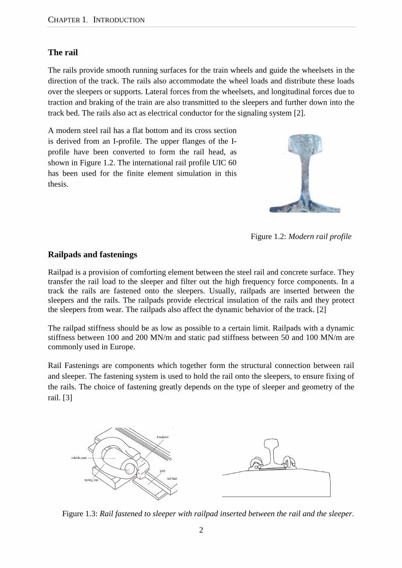
A modern steel rail has a flat bottom and its cross section
is derived from an I-profile. The upper flanges of the I-
profile have been converted to form the rail head, as
shown in Figure 1.2. The international rail profile UIC 60
has been used for the finite element simulation in this
thesis.
Figure 1.2: Modern rail profile
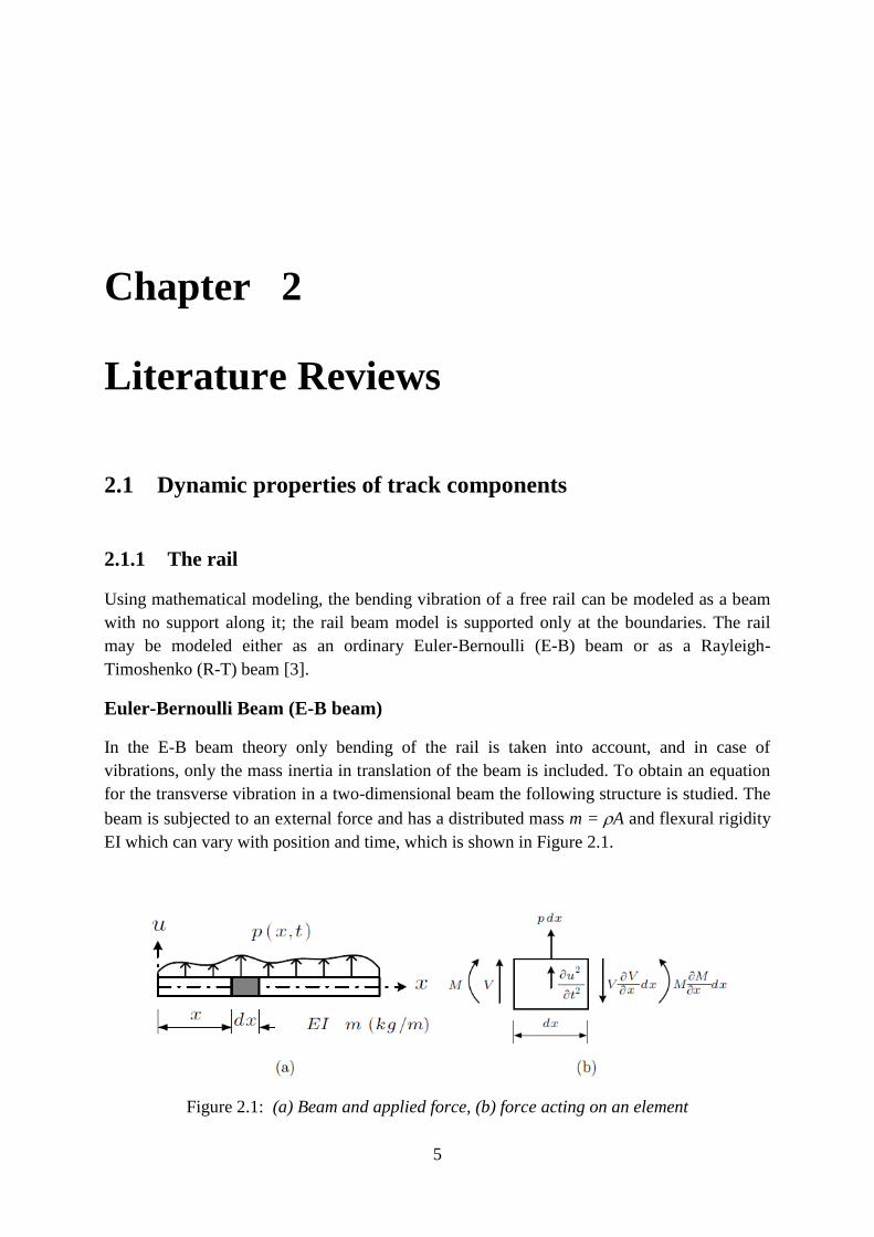
Railpads and fastenings
Railpad is a provision of comforting element between the steel rail and concrete surface. They
transfer the rail load to the sleeper and filter out the high frequency force components. In a
track the rails are fastened onto the sleepers. Usually, railpads are inserted between the
sleepers and the rails. The railpads provide electrical insulation of the rails and they protect
the sleepers from wear. The railpads also affect the dynamic behavior of the track. [2]
The railpad stiffness should be as low as possible to a certain limit. Railpads with a dynamic
stiffness between 100 and 200 MN/m and static pad stiffness between 50 and 100 MN/m are
commonly used in Europe.
Rail Fastenings are components which together form the structural connection between rail
and sleeper. The fastening system is used to hold the rail onto the sleepers, to ensure fixing of
the rails. The choice of fastening greatly depends on the type of sleeper and geometry of the
rail. [3]
Figure 1.3: Rail fastened to sleeper with railpad inserted between the rail and the sleeper.

1.2 PROPERTIES OF RAILWAY TRACK
3
The sleepers
The sleepers hold the rails and maintain tack gauge, level and alignment. They distribute and
transmit forces from the rail down to the ballast bed. Also they provide electrical insulation
between the two rails.[2]
For ballast railway track, there are wooden, steel and reinforced concrete sleepers available
nowadays. The choice usually depends on the speed of the train and economic reasons.
For standard gauge tracks, the optimum spacing is 0.60 m, which has been used for the
modeling in this thesis. There are mainly two types of concrete sleepers: Reinforced twin-
block sleepers and prestressed monoblock sleepers. In this thesis the later one was used.
Ballast and sub-ballast
The ballast is crushed granular material, of uniform size, placed as the top layer of the
substructure in which the sleepers are embedded. [4] The most important functions it
performs are resisting vertical, lateral, and longitudinal forces applied to the sleepers to
maintain track in its desired position, provision of resiliency and energy absorption for the
track, provision of drainage, and reduction of traffic induced stresses in the underlying layers,
and facilitating maintenance operations.
The sub-ballast is a granular layer between the ballast and subgrade which serves the purpose
of reducing the intensity of stress transmitted from the ballast layer to the subgrade and
facilitates drainage. In addition the sub-ballast layer prevents interpenetration of the subgrade
and ballast, prevents upward migration of fine material emanating from the subgrade and
helps prevent subgrade attrition by ballast.[4]
The main criterion for sub-ballast material to be used in railway track is that it should be
available locally and it should be free draining. A sub-ballast material should be coarse,
granular and well graded. Plastic fines are limited to maximum 5% and non-plastic fines to
maximum 12%. [5]
1.3 Aims of the Study
The aim of this thesis is to analyze the dynamic effects of the railway track. From the detailed
finite element models created in ABAQUS, more detailed information about the dynamic
effects of the railway track can be made, such as rail track vibration modes and receptance
functions. The results of the stabilizing system will be analyzed and suggestions will be made
for the further study.

CHAPTER 1. INTRODUCTION
4
1.4 Structure of the Thesis
A short description of each chapter is presented below to get an overview of the general
structure of the thesis.
In Chapter 2, selections of the literature reviews are presented, that constitute the basis of the
calculations in this thesis. It also briefly describes dynamic properties of the railway track
components and the models have been done by other people so far.
The well-known commercial software GEOTRACK and KENTRACK for railway track
system has been introduced in Chapter 3. The theories behind those programs have been
briefly explained and some of its limitations have been discussed.
The procedure of creating finite element models in ABAQUS/CAE is presented in Chapter 4.
The algorithms within ABAQUS that are used in this thesis are briefly presented and the
dynamic analysis approaches were explained.
The results of the finite element modeling in ABAQUS are presented in Chapter 5 and the
dynamic analyses are divided into frequency analysis, steady-state dynamic analysis and
explicit dynamic analysis. Vibration modes extracted from ABAQUS are demonstrated and
the dynamic properties of the railway track system have been studied through receptance
functions. By applying a moving load, the dynamic speed effect has been studied. The
displacement of the trackbed has been evaluated and compared to the measurement taken in
Sweden in the static analysis. At the end, comparison has been made between beam element
model and solid element model.
Chapter 6 contains a discussion of the results and presents the main results. Some
recommendations for further research are also suggested.
5
Chapter 2
Literature Reviews
2.1 Dynamic properties of track components
2.1.1 The rail
Using mathematical modeling, the bending vibration of a free rail can be modeled as a beam
with no support along it; the rail beam model is supported only at the boundaries. The rail
may be modeled either as an ordinary Euler-Bernoulli (E-B) beam or as a Rayleigh-
Timoshenko (R-T) beam [3].
Euler-Bernoulli Beam (E-B beam)
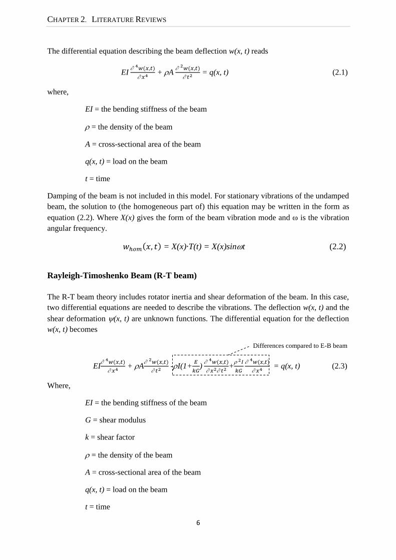
In the E-B beam theory only bending of the rail is taken into account, and in case of
vibrations, only the mass inertia in translation of the beam is included. To obtain an equation
for the transverse vibration in a two-dimensional beam the following structure is studied. The
beam is subjected to an external force and has a distributed mass m = A and flexural rigidity
EI which can vary with position and time, which is shown in Figure 2.1.
Figure 2.1: (a) Beam and applied force, (b) force acting on an element
CHAPTER 2. LITERATURE REVIEWS
6
The differential equation describing the beam deflection w(x, t) reads
EI
+ A
= q(x, t) (2.1)
where,
EI = the bending stiffness of the beam
= the density of the beam
A = cross-sectional area of the beam
q(x, t) = load on the beam
t = time
Damping of the beam is not included in this model. For stationary vibrations of the undamped
beam, the solution to (the homogeneous part of) this equation may be written in the form as
equation (2.2). Where X(x) gives the form of the beam vibration mode and is the vibration
angular frequency.
= X(x) T(t) = X(x)sint (2.2)
Rayleigh-Timoshenko Beam (R-T beam)
The R-T beam theory includes rotator inertia and shear deformation of the beam. In this case,
two differential equations are needed to describe the vibrations. The deflection w(x, t) and the
shear deformation (x, t) are unknown functions. The differential equation for the deflection
w(x, t) becomes
Differences compared to E-B beam
EI
+ A
-I(1+
)
+
= q(x, t) (2.3)
Where,
EI = the bending stiffness of the beam
G = shear modulus
k = shear factor
= the density of the beam
A = cross-sectional area of the beam
q(x, t) = load on the beam
t = time

2.1 DYNAMIC PROPERTIES OF TRACK COMPONENTS
7
If the shear deformation of the beam is suppressed, i.e. if one gives k a very large number,
then the two last terms on the left hand side tend to zero. Further, if the mass inertia in
rotation of the beam cross section is eliminated (noting that ρI = ρr2A = mr
2, and let r tend to
zero) then also the third term tends to zero and the E-B differential equation is obtained.
It was found that shear deformation of the rail can be neglected only for frequencies below
500 Hz. Dahlberg showed that at this frequency (500 Hz), and for a UIC60 rail, the Euler-
Bernoulli beam theory provides a vibration frequency that is 10 to 15 percent too high. [3]
Beam elements
Let a uniform beam lie on the x-axis. This 2d beam element has a node at each end and each
node has three degrees of freedom (D.O.F); axial translation, lateral translation and rotation,
as seen in Figure 2.2. Transverse shear deformations are taken into account by the
Timoshenko beam theory, which is usually applied when beam vibration is studied.
Figure 2.2: 2D beam element
The stiffness matrix for this Timoshenko beam element is defined as:
(2.4)
where,

CHAPTER 2. LITERATURE REVIEWS
8
(2.5)
Note that as an element becomes more and more slender,φy approaches zero. A/ky is the
effective shear area for transverse shear deformation in the transverse direction. The consisten
mass matrix for the beam element is:
(2.6)
2.1.2 The railpads and fastening
From a track dynamic point of view, the railpads play an important role. They influence the
overall track stiffness. A soft railpad permits a larger deflection of the rails when the track is
loaded by the train. Hence the axle load from the train is distributed over more sleepers.
Besides, since soft railpads can suppress the transmission of high-frequency vibrations down
to the sleepers and further down into the ballast, they also contribute to isolate high-frequency
vibration.[2]
The most commonly used physical model of a railpad is the spring-damper system. The
spring can be assumed to be linear, and the damping is assumed to be proportional to the
deformation rate of the railpad. According to the comparison between track models and
measurements it’s important to include the railpads to get an accurate track model. In the
measurements carried out before, it was found that soft railpads would result in lower sleeper
acceleration and higher railhead acceleration than the stiff railpads.
The stiffness of the fastening is normally much less than that of the railpad. Therefore, when
investing track dynamics the role of the fastenings is normally neglected.

2.1 DYNAMIC PROPERTIES OF TRACK COMPONENTS
9
2.1.3 The sleepers
Depending on which frequency interval is of interest, the concrete sleeper can be modeled as
either a rigid mass (at frequencies below 100 Hz) or as a flexible beam. For frequencies up to
300 or 400 Hz, the Euler-Bernoulli beam theory may suffice. At higher frequencies, the
Rayleigh-Timoshenko beam theory should be used for an accurate description of the sleeper
vibration. [3]
Along the rail, the stiffness changes because it is supported by sleepers separated by a
distance around 65 cm. The stiffness is higher when the wheel passes at the level of a concrete
sleeper. These vibrations induced by the sleeper distance have a frequency f given by the
equation where V is the speed of the train and D is the distance between two sleepers.
f =
(2.7)
2.1.3 The ballast, subballast and subgrade
The effect of the ballast is to distribute the loads from the sleepers to the soil. Usually, a layer
of subballast prevents the penetration of the ballast particles into the soil or vice versa.
Ballast is a complex medium because of its granular properties. The ballast is constituted by
stone particles. The behavior of the ballast is not well-known because of the complexity of the
interactions between particles. A granular media can have behavior both like solids and
liquids: on one hand, the ballast supports sleepers; on the other hand, the liquefaction of
ballast is a dangerous problem which can cause derailment. Without any train loadings,
internal forces in the ballast are low. During train passages, the friction between particles
increases and the ballast is compressed by the train loading. To provide safety against ballast
instability, the European and Swedish codes specified a limit of 3.5 m/s2 maximal vertical
deck acceleration (CEN, 2002 and The Swedish National Rail Administration, 2008). During
the measurements, it was checked if any particles move during train passages by painting
lines on the ballast, as shown in Figure 2.3.
At present, the state-of-the-art of track design concerning the ballast and the subgrade is
mostly empirical. The factors that control the performance of the ballast are poorly
understood. [3] The long-term behavior of the railroad track, including the ballast behavior
and the damage mechanics underlying the ballast settlement has been studied before. No
generally accepted damage and settlement equations or any material equations for the ballast
itself have been found. Only different suggestions to describe the ballast settlement from a
phenomenological point of view are available. A historical method for assessing track
performance is the use of track modulus.

CHAPTER 2. LITERATURE REVIEWS
10
Figure 2.3: Painting line on the ballast during measurements. Any particle displacement has
been observed
Ahlbeck developed the theory of the ballast pyramid model. In this model, the pressure
distribution is assumed to be uniform in a pyramid under sleepers and independent of the
depth. The friction between particles transmits the loading from the top layer to the bottom of
the ballast.[8]
Thus, the ballast is divided in one block for each sleeper (see Figure2.4). Each ballast block
can be modeled by a single degree-of-freedom system with a mass M, a stiffness K and a
damping C. Alhbeck suggests an internal friction angle for the ballast of 20° and 35° for the
subballast. To model the continuity of the ballast, shear stiffness and damping, connecting the
different blocks of the ballast, can be added.
Figure 2.4: Distribution of load from wheels to subballast [8]
2.1 DYNAMIC PROPERTIES OF THE TRACK
11
2.2 Dynamic Properties of the Track
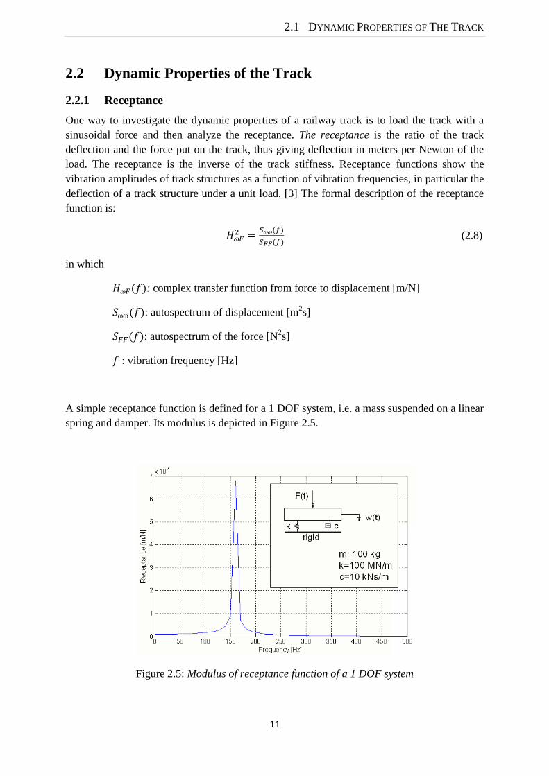
2.2.1 Receptance
One way to investigate the dynamic properties of a railway track is to load the track with a
sinusoidal force and then analyze the receptance. The receptance is the ratio of the track
deflection and the force put on the track, thus giving deflection in meters per Newton of the
load. The receptance is the inverse of the track stiffness. Receptance functions show the
vibration amplitudes of track structures as a function of vibration frequencies, in particular the
deflection of a track structure under a unit load. [3] The formal description of the receptance
function is:
(2.8)
in which
: complex transfer function from force to displacement [m/N]
: autospectrum of displacement [m2s]
: autospectrum of the force [N2s]
: vibration frequency [Hz]
A simple receptance function is defined for a 1 DOF system, i.e. a mass suspended on a linear
spring and damper. Its modulus is depicted in Figure 2.5.
Figure 2.5: Modulus of receptance function of a 1 DOF system

CHAPTER 2. LITERATURE REVIEWS
12
The dynamic equilibrium equation for this system yields:
C
+ K (t) = -M
+ F(t) (2.9)
By assuming the displacement function w(t)= , The solution of this equation could be
achieved:
=
(2.10)
Since the solution of this equation relates only to frequency if the mass, spring and damper
properties are constant with respect to time, and linear with respect to force and displacement.
Therefore it can be called the receptance function. It also can be expressed in a modulus H():
(2.11)
where,
: radial vibration frequency [rad/s]: =2
: eigenfrequency [rad/s]: =
: damping ratio [-]: =
The receptance functions always refer to a position, because they are basically transfer
functions. The analytical models allow calculating the receptance functions between the force
at a fixed position and any other position on the rail, the sleeper or the slab. These functions
are called cross-receptances, in contrast to the unique direct receptance, which applies to the
single position where the loading and displacement coincide. [6]
2.2.2 Resonance
Several well damped resonances can be found in a track structure. Figure 2.6 shows a typical
track receptances when rail is loaded with a sinusoidally varying force. Track receptance
when rail is loaded between two sleepers (full-line curve) and above one sleeper (dashed
curve) versus loading frequency. The maxima indicate resonance frequencies in the track
structure. Narrow resonance peak usually indicates the resonance at this frequency is very
highly damped.

2.1 DYNAMIC PROPERTIES OF THE TRACK
13
Figure 2.6: Typical track receptances when rail is loaded with a sinusoidally varying force.[3]
Sometimes when the track is built on a soft ground, one resonance may appear in the
frequency range 20 to 40 Hz. This is a resonance when the track and a great deal of the track
substructure vibrate on, for example, a layered structure of the ground.
One track resonance is usually obtained in the frequency range 50 to 300 Hz. This resonance
is obtained when the track structure (rails and sleepers) vibrates on the ballast bed. Another
resonance frequency can often be found in the frequency range 200 to 600 Hz. This resonance
is explained by the rail bouncing on the railpads.
The highest resonance frequency discussed here is the so-called pinned-pinned resonance
frequency. This is the resonance that can be seen at slightly less than 1000 Hz. The pinned-
pinned frequency occurs when the wavelength of the bending waves of the rail is twice the
sleeper spacing [3]. Pin-pin resonance is one of the most significant preferred vibration modes
of the beam, which are supported at equal distances, such as rails at sleepers in railway track
structures do. Pin-pin resonance is a vibration that appears in one basic (first) mode and
several higher modes, however the basic mode will have the highest amplitude. In operational
conditions of the railway, pin-pin resonance only partly influences wheel-rail contact of the
train while the speed dependent sleeper-passing frequency is more important. Among other
track resonance, pin-pin resonance plays an important role in noise and vibration radiation of
the rails and can be used as a meaningful instrument in track system dynamics recognition
and optimization. [9]
Figure 2.7: Pin-pin vibration mode

CHAPTER 2. LITERATURE REVIEWS
14
As a consequence of discretely supporting beams like rails, the rail in the track ‘frame-work’
will obtain vibration modes related to this type of supporting. The most important vibration
mode resembles a kind of bending between discrete points and pins. This mode is
schematically shown in Figure 2.7. With some simplifying assumptions, the pin-pin vibration
resonance occurs at a specific frequency (fpp), which can be calculated by:
fpp =
(2.12)
where:
l :distance between two supports [m]
EI : bending stiffness of rail (static) [Nm2]
m : mass of the rail per unit length [kg/m]
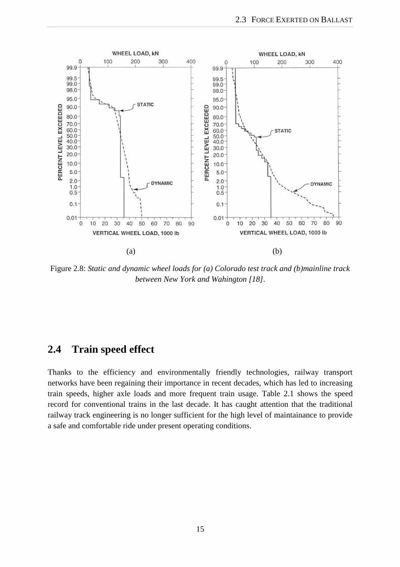
2.3 Forces exerted on ballast
There are two main forces which act on ballast. These are the vertical force of the moving
train and the “squeezing” force of maintenance tamping. The vertical force is a combination
of a static load and a dynamic component superimposed on the static load. The static load is
the dead weight of the train and superstructure, while the dynamic component, which is
known as the dynamic increment, depends on the train speed and the track condition. The
high squeezing force of maintenance tamping has been found to cause significant damage to
ballast. Besides these two main forces, ballast is also subjected to lateral and longitudinal
forces which are much harder to predict than vertical forces.[18]
The dead wheel load can be taken as the vehicle weight divided by the number of wheels. The
dynamic increment varies with train section as it depends on track condition, such as rail
defects and track irregularity. Figures 2.3 (a) and (b) show the static and dynamic wheel loads
plotted as cumulative frequency distribution curves for the Colorado test track and the
mainline track between New York and Washington respectively.[18]The static wheel load
distribution was obtained by dividing known individual gross car weights by the
corresponding number of wheels, and the dynamic wheel load distribution was measured by
strain gauges attached to the rail. The vertical axes of the two figures give the percentage of
total number of wheel loads out of 20,000 axles which exceed the load on the horizontal axis.
Clearly, the dynamic increment is more noticeable for high vertical wheel loads and is more
significant for the mainline track between New York and Washington than the Colorado test
track. This is due to the almost perfect track condition for the Colorado test track. It was also
noticed that the high dynamic load for the mainline track between New York and Washington
occurred at high speeds.[18]
2.3 FORCE EXERTED ON BALLAST
15
(a) (b)
Figure 2.8: Static and dynamic wheel loads for (a) Colorado test track and (b)mainline track
between New York and Wahington [18].
2.4 Train speed effect
Thanks to the efficiency and environmentally friendly technologies, railway transport
networks have been regaining their importance in recent decades, which has led to increasing
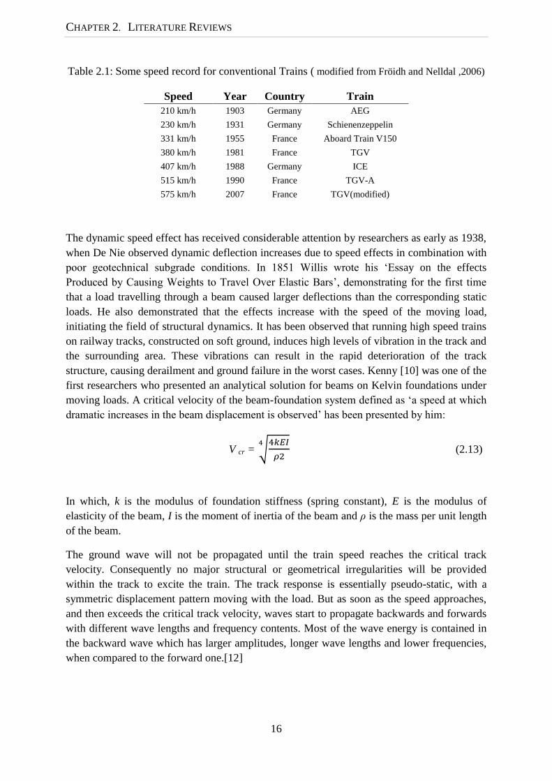
train speeds, higher axle loads and more frequent train usage. Table 2.1 shows the speed
record for conventional trains in the last decade. It has caught attention that the traditional
railway track engineering is no longer sufficient for the high level of maintainance to provide
a safe and comfortable ride under present operating conditions.
CHAPTER 2. LITERATURE REVIEWS
16
Table 2.1: Some speed record for conventional Trains ( modified from Fröidh and Nelldal ,2006)
Speed Year Country Train
210 km/h 1903 Germany AEG
230 km/h 1931 Germany Schienenzeppelin
331 km/h 1955 France Aboard Train V150
380 km/h 1981 France TGV
407 km/h 1988 Germany ICE
515 km/h 1990 France TGV-A
575 km/h 2007 France TGV(modified)
The dynamic speed effect has received considerable attention by researchers as early as 1938,
when De Nie observed dynamic deflection increases due to speed effects in combination with
poor geotechnical subgrade conditions. In 1851 Willis wrote his ‘Essay on the effects
Produced by Causing Weights to Travel Over Elastic Bars’, demonstrating for the first time
that a load travelling through a beam caused larger deflections than the corresponding static
loads. He also demonstrated that the effects increase with the speed of the moving load,
initiating the field of structural dynamics. It has been observed that running high speed trains
on railway tracks, constructed on soft ground, induces high levels of vibration in the track and
the surrounding area. These vibrations can result in the rapid deterioration of the track
structure, causing derailment and ground failure in the worst cases. Kenny [10] was one of the
first researchers who presented an analytical solution for beams on Kelvin foundations under
moving loads. A critical velocity of the beam-foundation system defined as ‘a speed at which
dramatic increases in the beam displacement is observed’ has been presented by him:
V cr =
(2.13)
In which, k is the modulus of foundation stiffness (spring constant), E is the modulus of
elasticity of the beam, I is the moment of inertia of the beam and ρ is the mass per unit length
of the beam.
The ground wave will not be propagated until the train speed reaches the critical track
velocity. Consequently no major structural or geometrical irregularities will be provided
within the track to excite the train. The track response is essentially pseudo-static, with a
symmetric displacement pattern moving with the load. But as soon as the speed approaches,
and then exceeds the critical track velocity, waves start to propagate backwards and forwards
with different wave lengths and frequency contents. Most of the wave energy is contained in
the backward wave which has larger amplitudes, longer wave lengths and lower frequencies,
when compared to the forward one.[12]

2.4 TRAIN SPEED EFFECT
17
An observation of important soft soil site at Ledsgard in Sweden has been carried out by
Madshus & Kaynia (2000) and Madshus et al. (2004), as shown in Figure 2.9. Measurements
at speed of 45 mph revealed a typical quasi-static track response with every axle having its
own footprint. The response changed completely with the increasing speed. At 115mph, the
displacement amplitude drastically increased and the displacement pattern became
asymmetrical with a tail of free oscillations following the train.
Figure 2.9: Maximum measured normalized displacement versus speed [12]
2.4 Mathematical model
2.5.1 Beam on elastic foundation (BOEF) model
In a historic view, the BOEF model is by far The Classic Method and also forms the backbone
of many subsequent improvements made to track design (See Figure 2.10). This model was
introduced by Winkler in 1867 and is still in use for easy and quick track deflection
calculations [11].
k
EI Rail beam
Figure 2.10: Beam (bending stiffness EI) on elastic foundation (bed modulus k)

CHAPTER 2. LITERATURE REVIEWS
18
The model has a sound mathematical formulation with quite clear simple physical
interpretation. It assumes the rail modeled as an infinite Euler-Bernoulli beam with a
continuous longitudinal support from a Winkler foundation, which may be regarded as
equivalent to an infinite longitudinal line of vertical, uncoupled and elastic springs. The
distributed force supporting the beam then is proportional to the beam deflection. By only
using two track parameters the rail deflection w(x) could be obtained from the differential
equation
EI
+ k w(x) = q(x) (2.14)
where,
x = the length coordinate
q(x) = the distributed load on the rail
EI = the beam bending stiffness EI (Nm2)
k = the foundation stiffness (N/m2, i.e. N/m per meter of rail).
This model may be acceptable only for static loading of a track on soft support, for example a
track with wood sleeper. Several evident limitations are inherent in the BOEF model. Such as
the fundamental problem of circular definition when measuring k, which is not very helpful
for the predictability; the assumption of continuous foundation and the response of the track is
linear; materials behavior only in the vertical direction; shear deformation in the rails is not
included ; continuously welded rail are assumed ; no time dependent.
Another prominent limitation is BOEF model tacitly assumes that tensile stress can develop in
exactly the same way as compressive stresses on the interface between the sleepers and the
rest of the foundation. It can be seen when using this model that the track is lifted both in
front of and behind the wheel. Since this cannot be physically valid for granular materials,
there is a need for tensionless track model. Such models are nonlinear since the length of
contact zone cannot be known in advance and will vary dependent upon the size of the load.
2.5.2 Beam (rail) on discrete supports
In this model the supports could either be discrete spring-damper systems or spring-mass-
spring systems, modeling railpads, sleepers and ballast bed. In a three-dimensional model, the
rail (a beam element) is placed on a spring and damper in parallel. This spring-damper system
models the railpad. Below this another beam element, modeling the sleeper, is placed. The
sleeper rests on an elastic foundation, i.e. another spring –damper system, as shown in Figure
2.11. [7]

2.4 MATHEMATICAL MODEL
19
Sleeper
Rail beam
Track bed
Winkler type
(a) Longitudinal view
Rail beam
Sleeper beam
(b) Transverse view
Figure 2.11: Rail on discrete support
2.5.3 Discretely supported rail including ballast mass
To be able to add a resonance frequency at low frequency (20 to 40 Hz) to the model
described above, Oscarsson [13] incorporated more masses into the model, see Figure 2.9. By
making the ballast and subgrade mass large (much larger than the sleeper and rail mass) and
by adjusting the subgrade stiffness, a resonance at low frequency can be achieved. Then,
essentially, the ballast-subgrade masses vibrate on the subgrade stiffness. It is noted in Figure
2.9 that there are connections between the ballast and subgrade masses, implying that a
deflection at one point (at one sleeper) will influence the deflection at the adjacent sleepers.
This phenomenon (which is there in a real track) cannot be modeled with the simpler models
such as the track model in Figure 2.10. The influence of the ballast density on the wheel-rail
contact force at a rail joint and the ballast acceleration could also be studied by this model [3].
Sleeper mass
Rail beam
Ballast and Subgrade mass
Railpad stiffness and damping
Ballast stiffness and damping
Subgrade stiffness and damping
Figure 2.12: Rail on discrete supports with rigid masses modeling the sleepers.

CHAPTER 2. LITERATURE REVIEWS
20
2.5.4 Tensionless BOEF model according to Kjell Arne Skoglund
The vertical downwards force at the rail-wheel contact points tends to lift up the rail and
sleeper some distance away from the contact point, as shown in Figure 2.13. The uplift force
depends on the wheel loads and self-weight of the superstructure. As the wheel advances, the
lifted sleeper is forced downwards causing an impact load, which increases with increasing
train speed. This movement causes a pumping action in the ballast, which increases the ballast
settlement by exerting a higher force on the ballast and causing “pumping up” of fouling
materials from the underlying materials in the presence of water. [18]
Figure 2.13: Uplift of rails [18]
One remarkable tension-free model was developed based on adding equal but opposite loads
to the BOEF model in the regions where uplift occurs by Kjell Arne Skoglund. [11] Also, the
weight of the track ladder is incorporated. As expected, the model shows that the length of the
uplift zone and amount of uplift have higher values than predicted by the BOEF model. The
model may be useful when considering contact problems in track, for instance in a buckling-
of rails analysis. This approach is equivalent to the more formal method by Tsai and
Westmann. Compared to the traditional BOEF model this model is an improvement, however,
it still suffers from other BOEF limitations.

2.4 MATHEMATICAL MODEL
21
2.5.5 Pasternak foundation
This model assumes shear interactions
between the Winkler springs. This may be
accomplished by connecting the ends of the
springs to the beam consisting of
incompressible vertical elements which then
only deforms by transverse shear. In Figure
2.14 the classical rail element on a Winkler
foundation is extended with a shear element
representing the interaction between the
springs. The shear element is connected to the
rail element. The distributed load on the rail is
assumed to be zero [2]
Figure 2.14: Pasternak foundation for beam
2.5.6 Other rail track models
Filonenko-Borodich foundation
The interaction between the foundation springs is obtained by connecting the top ends to a
stretched elastic membrane with a constant tension field T. The equilibrium in vertical
direction of a beam element was taken.
Reissner foundation
Starting with the equations of a continuum, Reissner then assumes the horizontal stresses (in-
plane stresses) in the foundation layer to be negligibly small compared to the vertical stresses.
Also the horizontal displacements of the upper and lower boundaries of the foundation layer
are assumed to be zero.
Vlasov and Leontiev approach
This model handles the problem by processing an unknown function that contains a
differential equation. The displacements are represented by finite series where each term is a
product of the function. Through a variational process a differential equation in the unknown
function is arrived at the solution of this equation will eventually solve the problem.

CHAPTER 2. LITERATURE REVIEWS
22
A simple Euler-Bernoulli beam element model
The rail is discretely supported by the sleepers. Two models have been developed one
ordinary model with linear spring support in both tension and compression, and another
model with linear spring support only in the compression model. The latter one could be said
to be a ‘no tension’ model [11].
Figure 2.15: Beam element model of a track section.
Model according to Adin
Adin has solved the no-tension problem by using beam elements with exact stiffness matrices
especially developed for a beam on a Winkler foundation. The problem to be solved is of a
more general nature than that of Tsai and Westmann as several zones of uplift are allowed.
Figure 2.16: General deflection of a beam on elastic foundation.
2.4 MATHEMATICAL MODEL
23
Beam element model with nonlinear support
This model was developed by Kjell Arne Skoglund, which is motivated by the fact that the
load-deflection curve for a railway track is often, if not always, nonlinear. The nonlinear
behavior is usually of the hardening type with increasing track stiffness as the load increases.
In such a model the track stiffness must be regarded as the derivative of the load with respect
to deflection. The capabilities of the new model have not been fully explored. In the future,
this model will hopefully provide a conceptually simple but still more accurate tool,
especially when the track shows a clear nonlinear load-deformation relationship.[11]

24
25
Chapter 3
Available Programs
Based on the assumption of elastic behavior of substructure materials, several multilayer track
models have been developed for analysis of stress in the track and subgrade. Examples of
these models include GEOTRACK and KENTRACK.
3.1 GEOTRACK
3.1.1 Geotrack components
As one of the most well known 3D static track system model, Geotrack is a great design aid
for railway track.. It was developed to emphasize the geotechnical aspects of track
behavior.The rails are represented as linear elastic beams supported by a number of
concentrated reactions, one at each intersection of tie and rail. The rails span 11 ties and are
free to rotate at the ends and at each tie. The parameters describing the rails are cross-
sectional area, moment of inertia, and material modulus of elasticity. The connection between
the rail and tie is represented by a linear spring, with a specified spring constant, which can
take tension as well as compression. [14] The ties are represented as linear elastic beam also
specified by modulus of elasticity, cross-sectional area, and moment of inertia. Each tie is
divided into 10 equal rectangular segments with the underlying ballast reaction represented as
a concentrated force in the center of each segment. These forces are applied to the ballast
surface as a uniform pressure over a circular area whose size is related to the tie segment
dimensions.[14]

CHAPTER 3. AVAILABLE PROGRAMS
26
One important assumption made in Geotrack is that each wheel load, when applied over a
central tie, is distributed over 11 ties, five on each side of the central tie. Any tie at a distance
of six or more ties away from the central tie does not carry any load, as shown in Figure 3.2.
This assumption is reasonable for design purposes since the most critical stress and strain lie
in the vicinity of the central tie. It allows the application of the simple superposition principle
to determine the stresses and strains under multiple wheel loads and thus saves a great deal of
computer time.
Up to 4 superimposed vertical axle loads could be applied on the rails. Analysis of induced
stress and deformation in substructure could be carried out. The output mainly contains three
parts:
Superstructure
Rail and tie deflections
Rail seat load
Rail and tie bending moments
Tie/Ballast reaction
Substructure
Vertical deflection
Complete stress state
Deviator stress
Bulk stress
Principal stresses and directions
Track modulus for the combined system
3.1.2 Stress-dependent material properties
Geotrack utilizes the work of Burmister which put forward a general theory of stresses and
displacements in layered systems to set up the multiple layer stress dependent elastic
system.[14] In conjunction with this the material properties for each layer are calculated based
upon a relation in the form of:
Er = k1 k2 (3.1)
where,
Er = the vertical resilient modulus
= the sum of initial and incremental bulk stress (i.e. maximum bulk stress)

3.1.3 VALIDATION OF GEOTRACK
27
k1, k2 = parameter determined experimentally
The parameters in the k-theta relation are not dimensionless. Because of this Geotrack
modifies Equation (3.1) to the form:
Er = k3
(3.2)
where,
Pa = atmospheric pressure
= mean stress
k3, k4 = Parameters determined experimentally
Since the model is elastic, Poisson’s ratio is also a required input parameter and because the
formulations require each layer of the system to have a single elastic modulus a weighted
average at the mid depth value for each layer is assigned. Such simplifications reduced
computing power requirements, albeit at the expense of accuracy.
3.1.3 Validation of Geotrack
Geotrack was developed at the University of Massachusetts, Amherst, USA in the late 70s
and early 80s. After considering the other programs available at the time, Geotrack grew from
improvements to a program known as MULTA (Multi Layer Track Analysis). Validation was
provided by comparing Geotrack outputs with data taken from tests carried out at The (US)
Department of Transportation’s Facility for Accelerated Service Testing (FAST) in Pueblo,
Colorado, USA.
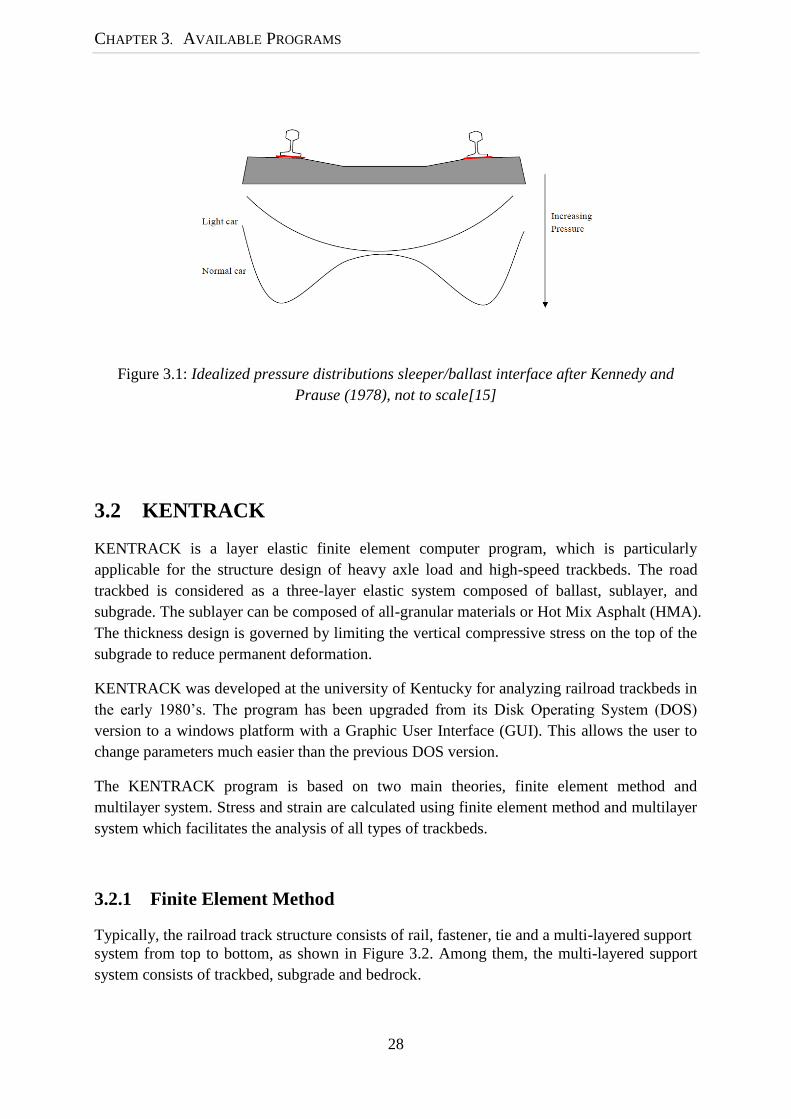
One of the most important validations of Geotrack was its ability of reproducing test results of
the pressure distributions at the interfaces between sleeper and ballast, as shown in Figure 3.1,
and between ballast and subgrade.[15]
The development of the w-shaped pressure distribution for a normal car occurs theoretically
when a flexible sleeper is supported continuously by an elastic layer of uniform stiffness. In
practice this is a gross simplification because sleeper support is highly erratic due to the
relatively large size of ballast particles and the development of structure within the structure.
CHAPTER 3. AVAILABLE PROGRAMS
28
Figure 3.1: Idealized pressure distributions sleeper/ballast interface after Kennedy and
Prause (1978), not to scale[15]
3.2 KENTRACK
KENTRACK is a layer elastic finite element computer program, which is particularly
applicable for the structure design of heavy axle load and high-speed trackbeds. The road
trackbed is considered as a three-layer elastic system composed of ballast, sublayer, and
subgrade. The sublayer can be composed of all-granular materials or Hot Mix Asphalt (HMA).
The thickness design is governed by limiting the vertical compressive stress on the top of the
subgrade to reduce permanent deformation.
KENTRACK was developed at the university of Kentucky for analyzing railroad trackbeds in
the early 1980’s. The program has been upgraded from its Disk Operating System (DOS)
version to a windows platform with a Graphic User Interface (GUI). This allows the user to
change parameters much easier than the previous DOS version.
The KENTRACK program is based on two main theories, finite element method and
multilayer system. Stress and strain are calculated using finite element method and multilayer
system which facilitates the analysis of all types of trackbeds.
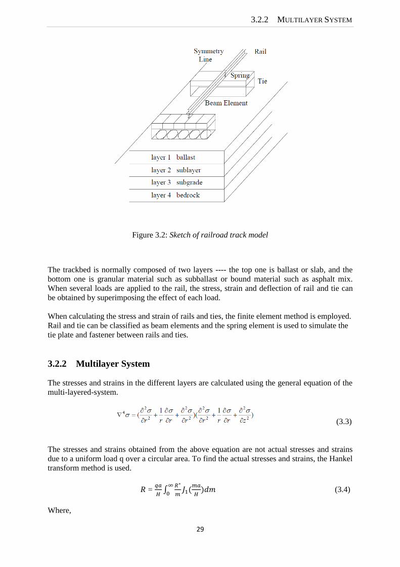
3.2.1 Finite Element Method
Typically, the railroad track structure consists of rail, fastener, tie and a multi-layered support
system from top to bottom, as shown in Figure 3.2. Among them, the multi-layered support
system consists of trackbed, subgrade and bedrock.
3.2.2 MULTILAYER SYSTEM
29
Figure 3.2: Sketch of railroad track model
The trackbed is normally composed of two layers ---- the top one is ballast or slab, and the
bottom one is granular material such as subballast or bound material such as asphalt mix.
When several loads are applied to the rail, the stress, strain and deflection of rail and tie can
be obtained by superimposing the effect of each load.
When calculating the stress and strain of rails and ties, the finite element method is employed.
Rail and tie can be classified as beam elements and the spring element is used to simulate the
tie plate and fastener between rails and ties.
3.2.2 Multilayer System
The stresses and strains in the different layers are calculated using the general equation of the
multi-layered-system.
(3.3)
The stresses and strains obtained from the above equation are not actual stresses and strains
due to a uniform load q over a circular area. To find the actual stresses and strains, the Hankel
transform method is used.
R =
(3.4)
Where,

CHAPTER 3. AVAILABLE PROGRAMS
30
stress or displacement due to loading which can be expressed as – mJ0(α)
R = stress or displacement due to load q
J = Bessel function
M = parameter
3.2.3 Material Properties
Ballast can be considered as either a linear or non-linear material. When a railroad is recently
constructed and has not been compacted, ballast always behaves non-linearly. In this case, the
constitute equation for calculating the resilient modulus of granular materials is governed by
the following two eaqutions:
E = K1 (3.5)
θ= σ1+ σ2+ σ3+γz(1+2K0) (3.6)
where, E is the resilient modulus; K1 and K2 are the coefficients; σ1, σ2 and σ3 are the three
principle stresses; γ is the unit weight of materials and K0 is lateral stress ratio.
Subgrade is always considered to be a linearly elastic material. The bottommost layer is
generally the bedrock which is considered to be impressible with a Poisson’s ratio of 0.5.
3.3 Limitations of available programs
There are several evident limitations that are inherent in the Geotrack model and Kentrack
model. It is important to be aware of these restrictions in an actual design process in order to
avoid using the method in situations where it is not appropriate. The most prominent aspects
that can be questionable may be described as follows:
Possibility of missing maximum values.
A major drawback of Geotrack is that the rail load is not applied to the tie directly above one
of the reactive points between the tie and the layered system. As a result, the stresses and
strains computed in the layered system are those under the reactive points, instead of those
under the rail load, which are usually the most critical. In other words, Geotrack may miss
maximum values and result in a critical stress or strain which is too small.
Continuously welded rails with certain length.
In Geotrack, rails are considered as integral beams with relative short length, and are not
divided into finite elements. Consequently, they must be homogeneous and uniform in cross
3.3 LIMITATIONS OF AVAILABLE PROGRAMS
31
section and cannot have joints or discontinuities. This assumption justifies the ability of
bending moment to be transferred in the rails. However, it is not possible to account for the
effect of joints, and Esveld [2] has the expression for such a track. Besides, some responses
may be not able to be observed due to the short length of the rail. .
No time dependent.
Dynamic loads are due to acceleration which arises because of irregularities in the geometry
of the wheels and rails and variability in the load/response of the support. It is evident that the
track is subjected to dynamic loading when trains pass over it, and especially so if the train
speed is high and the foundation is soft. Neither Geotrack model nor Kentrack model says
anything about time dependent or dynamic behavior of the track.
Elastic homogeneous continuum assumption.
Even though in Geotrack the stess-dependent material properties of ballast and subgrade soil
have been used. However, the track system is still based on assuming the railroad ballast bed
to be an elastic homogeneous continuum by defining the unbound aggregate layers through
Elastic Modulus and Possion’s ratio. The elastic modeling can be used to estimate the
behaviour of materials prior to failure, but it is incapable of predicting materials behaviour for
stress that exceed the yield limit. Using of linear elastic analysis to represent soil behaviour is
inappropriate and can lead to misleading results.
Mohamed A. shahin studied the effect of elastoplasticity in the design of railway tracks. An
elastoplastic (Mohr-Coulomb) 3D model was performed and compared with the 3D elastic
model. [16] The results show that higher vertical displacement and stress along track depth
will be predicted with the elastoplastic analysis. Mohamed explained this is because the
elastoplastic analysis allows plastic deformation to develop and plastic failure to occur.
Actually this kind of simulation is still not realistic enough for the analysis of real ballast
behaviour like ballast movement,deformation and degradation. Neither does it take account of
the factors affecting ballast strength and stability like ballast aggregate gradation, aggregate
shape properties, and loading characters.
To satisfy this need, discrete element method could be used, as shown in Figure 3.3. A DEM
model simulates the mechanical response of a particulate medium by explicitly accounting for
the dynamics of each particle in the system. [17]

CHAPTER 3. AVAILABLE PROGRAMS
32
(a) Discrete element analysis (b) Continuum analysis
Figure 3.3: Comparation between discrete element and continuum analysis
No lateral force.
The lateral force is the force that acts parallel to the long axis of the sleepers. The principal
sources of this type of force are lateral wheel force and buckling reaction force. The lateral
wheel force arises from the train reaction to geometry deviations in self-excited hunting
motions which result from bogie instability at high speeds, and centrifugal forces in curved
tracks. [18] Geotrack model and Kentrack model can be useful when considering the vertical
track behavior. But when it comes to the lateral direction, this model is oversimplified and is
not capable of providing any data.

33
Chapter 4
Creating Finite Element Models
This chapter deals with the modeling techniques that are used to analyze the railway track in
the commercial software ABAQUS. A brief summary of the routines that have been used are
presented. The finite element models were created in ABAQUS/CAE which includes the
Graphical User Interface (GUI). This method of creating models is easier than coding an input
file, especially when the models are large, as in the case with 3D models.
4.1 Modeling Procedures in ABAQUS/CAE
The ABAQUS/CAE environment is divided into different modulus, where each module
defines a logical aspect of the modeling process; for instance, defining the geometry, defining
the material properties, and generating a mesh. The GUI interface generates an input file with
all information of the model, to be submitted to the solver, using ABAQUS/Standard or
ABAQUS/Explicit routines. The solver performs the analysis and sends the information back
to ABAQUS/CAE for evaluation of the results.
4.1.1 Modules
Most models created in ABAQUS/CAE are assembled from different parts. It always starts
with creating different parts separately in the parts module. Different parts may need different
material properties, which are defined in the property module. A full range of material
properties are available in ABAQUS, such as elastic and plastic behavior, as well as thermal
and acoustic behavior. The model then is assembled in the assembly model, by combing the
different instances originates from different parts. In the step module the analysis is divided in
different analysis step, such as static and dynamic analyses. These can be combined in a way
to resemble the physical problem that is to be analyzed. The instances in the model will not
interact with each other until they have been connected in the interaction module. Connector
elements can be defined, to simulate for example spring or dashpot behavior. The loads acting

CHAPTER 4. CREATING FINITE ELEMENT MODELS
34
on the model are defined in the load module, as well as boundary conditions. The load and
boundary conditions can be defined to vary over time as well as over different steps. The
whole model is then meshed in the mesh module. The meshing techniques vary with the
element type and the geometry of the model.[19]
4.2 Elements
Abaqus has an extensive element library to provide a powerful set of tools for solving many
different problems. All elements used in ABAQUS are divided into different categories,
depending on the modeling space. The element shapes available are beam elements, shell
elements and solid elements and the modeling space is divided into 3D space, 2D planar space
and axisymmetric space. Some examples of types of finite elements are shown in Figure 4.1
below.
Figure 4.1: Examples of different types of finite elements (nodes and dofs indicated by small
circles and small arrows, respectively): a) Two-noded linear truss element (for axial loads
only), b) Beam element that allows axial, transversal and moment loads, c) Four-noded 2D
element, d) Eight-noded 2D element, e) 20-noded 3D element and f) 27-noded 3D element
(with local coordinate system indicated through the centre node). (Elements e) and f) with
only three of the dofs displayed.)
4.2.1 Beam elements
Beam elements have been used for the rails and sleepers modeling. A beam element is an
element in which assumption are made so that the problems reduced to one dimension

4.2 ELEMENTS
35
mathematically. The primary solution variable is then functions of the length direction of the
beam. For this solution to be valid, the length of the element must be large compared to its
cross-section. There are two main types of beam elements formulations, the Euler-Bernoulli
theory and the Timoshenko theory, which have been discussed in Chapter 2.
The Euler-Bernoulli theory assumes that the plan cross-sections, initially normal to the beam
axis, remain plane, normal to the beam axis, and undistorted. All beam elements in ABAQUS
that use linear or quadratic interpolation are based on this theory. The Timoshenko beam
theory allows the elements to have transverse shear strain, so that the cross-sections don’t
have to remain normal to the beam axis. This is generally more useful for thicker beams.[1]
4.2.2 Solid element
Solid elements in two and three dimensions are available in ABAQUS. The two-dimensional
solid element allows modeling of plane and axisymmetric problems. In three dimensions the
isoparametric hexahedron element is the most common, but in some cases complex geometry
may acquires tetrahedron elements. Those elements are generally only recommended to fill in
awkward parts of mesh. ABAQUS provides both first-order linear and second-order quadratic
interpolation of the solid elements. The first-order elements are essentially constant strain
elements, while the second-order elements are capable of representing all possible linear
strain fields and are more accurate when dealing with more complicated problems. [1]
4.2.3 Rigid elements
For the discretely supported track including ballast mass model, the ballast is modeled as rigid
element since only its mass is concerned. A rigid part represents a part that is so much stiffer
than the rest of the model that its deformation can be considered negligible. Computational
efficiency is the principal advantage of rigid parts over deformable parts. During the analysis
element-level calculations are not performed for rigid parts. Although some computational
effort is required to update the motion of the rigid body and to assemble concentrated and
distributed loads, the motion of the rigid body is determined completely by the reference
point. There are two kinds of rigid parts: discrete rigid part and analytical rigid part. When
describing a rigid part an analytical rigid part will have the priority because it is
computationally less expensive than a discrete rigid part.[1]
4.2.4 Spring and Dashpot elements
Spring and dashpot elements are widely used in this model. For instance, the railpads between
the rail and the sleeper, connectors for bounding adjacent ballasts in each direction, and the
boundary conditions for constraining the sleepers. SPRING1 and SPRING2 elements are
available only in Abaqus/Standard. SPRING1 is between a node and ground, acting in a fixed
direction. SPRING2 is between two nodes, acting in a fixed direction. The SPRINGA element
is available in both Abaqus/Standard and Abaqus/Explicit. SPRINGA acts between two

CHAPTER 4. CREATING FINITE ELEMENT MODELS
36
nodes, with its line of action being the line joining the two nodes, so that this line of action
can rotate in large-displacement analysis. The spring behavior can be linear or nonlinear in
any of the spring elements in Abaqus.[1]
4.3 Analysis Type
4.3.1 Linear Eigenvalue Analysis
Linear eigenvalue analysis is used to perform an eigenvalue extraction to calculate the natural
frequencies and corresponding mode shapes of the model. The analysis can be performed
using two different eigensolver algorithms, Lanczos or subspace. The Lanczos eigensolver is
faster when a large number of eigenmodes are required while the subspace eigensolver can be
faster for smaller systems. When using the Lanczos eigensolver, one can choose the range of
the eigenvalues of interested while the subspace eigensolver is limited to the maximum
eigenvalue of interest.[1]
4.3.2 Steady-state Dynamic Analysis
One way to investigate the dynamic properties of a railway track is to load the track with a
sinusoidal force. At frequencies up to about 200Hz, this can be done by using hydraulic
cylinders. If one wants to investigate the track response at higher frequencies, the track may
be excited by an impact load, for example from a sledge-hammer. [3]
In ABAQUS steady-state dynamic analysis provides the steady-state amplitude and phase of
the response of a system due to harmonic excitation at a given frequency. Usually such
analysis is done as a frequency sweep by applying the loading at a series of different
frequencies and recording the response; in Abaqus/Standard the direct-solution steady-state
dynamic procedure conducts this frequency sweep. In a direct-solution steady-state analysis
the steady-state harmonic response is calculated directly in terms of the physical degrees of
freedom of the model using the mass, damping, and stiffness matrices of the system. [1]
By editing the keyword after create the model, the amplitude of the rail vibration in steady-
state dynamic analysis could be obtained.
4.3.3 General Static Analysis
The general static analysis can involve both linear and nonlinear effects and is performed to
analyse static behavior such as deflection due to a static load. A criterion for the analysis to be
possible is that it is stable. A static step uses time increments, not in a manner of dynamic
steps but rather as a fraction of the applied load. The default time period is 1.0 units of time,

4.3 ANALYSIS TYPE
37
representing 100% of the applied load. The nonlinear effects are expected, such as large
displacements, material nonlinearities, boundary nonlinearities, contact or friction, the
NLGEOM command should be used. When dealing with an unstable problem, such as in
buckling or collapse, the modified Risk method can be used. It uses the load magnitude as an
additional unknown, and solves simulations for loads and displacements. This method
provides a solution even if the problem is nonlinear.[19]
4.3.4 Dynamic Implicit Analysis
The dynamic implicit analysis method is used to calculate the transient dynamic response of a
structure. A direct-integration dynamic analysis in Abaqus/Standard must be used when
nonlinear dynamic response is being studied. The general direct-integration method provided
in Abaqus/Standard, called the Hilber-Hughes-Taylor operator, is an extension of the
trapezoidal rule. The half-step residual is the equilibrium residual error halfway through a
time increment, t + Δt/2 and once the solution at t + Δt has been obtained, the accuracy of the
solution can be accessed and the time step adjusted appropriately. The principal advantage of
the Hilber-Hughes-Taylor operator is that it is unconditionally stable for linear systems; there
is no mathematical limit on the size of the time increment that can be used to integrate a linear
system.This nonlinear equation solving process is expensive; and if the equations are very
nonlinear, it may be difficult to obtain a solution. However, nonlinearities are usually more
simply accounted for in dynamic situations than in static situations because the inertia terms
provide mathematical stability to the system; thus, the method is successful in all but the most
extreme cases.[1]
The choice of the time increment depends on the type of analysis performed. In dynamic
problems, a smaller time increment than the stable one might be used, to get an accurate result
depending on the variations in the structure. There are two ways of defining the time
increment: automatic or fixed incrementation. The automatic incrementation scheme is
provided for use with the general implicit dynamic integration method. The scheme uses a
half-step residual control to ensure an accurate dynamic solution. By defining initial,
minimum, and maximum increment sizes the automatic time increments can be chosen. If no
convergence is achieved, a smaller one is used until convergence is achieved, down to the
minimum increment defined.[1]

38

39
Chapter 5
Modeling Results
The results from the finite element modeling in ABAQUS are presented. The purpose of the
modeling is to study the dynamic properties of the railway track.
Three dynamic analyses have been carried out: Frequency extraction, Steady-state dynamic
analysis and Dynamic explicit analysis. Some examples of lateral and vertical vibration
modes have been presented. A direct receptance curve has been achieved in the steady-state
dynamic analysis by applying a harmonic load on the middle of the rail, which has been used
as a criterion for the research of different track components dynamic effect. Train speed effect
has been studied by implementing dynamic explicit analysis. The displacement of the
trackbed has been evaluated and compared to the measurement taken in Sweden in the static
analysis.
5.1 Beam (rail) on discrete supports Model
5.1.1 Track properties
One Beam (rail) on discrete supports model was created in ABAQUS as shown in Figure 5.1.
The rail (a beam) was placed on a spring and damper in parallel. This spring-damper system
models the railpad. Below this another beam element, modeling the sleeper, is placed. The
sleeper rests on an elastic foundation, i.e. another spring-damper system. Track properties
used for ABAQUS modeling are listed in Table 5.1. The rail and sleeper cross-section
dimensions that have been used are shown in Figure 5.2.
The international rail profile UIC 60 has been chosen for the simulation. Due to the fact that
it’s unable to assign sketch profile to beam element in ABAQUS, approximation I-shape rail
profile has been used. Compared to the actual rail profile the deviation of the approximation is
less than 0.6% , which is neglectable. For instance, the area moment of inertia Ixx for the
actual and approximation rail profile is 3.055*10-5
m4
and 3.072*10-5
m4 respectively.

CHAPTER 5. MODELLING RESULTS
40
Figure 5.1:Beam on discrete support model created in ABAQUS
Table 5.1: Track properties used for ABAQUS modeling
Material Property Track Component
Rail Sleeper Ballast
Modulus of elasticity, E (GPa) 207 70 N/A
Poisson's ratio, 0.28 0.3 N/A
Unit weight, (kg/m3) 7850 2400 54
Spacing (m) 1.4 0.6 0.04
Thickness (m) 0.182 0.2 0.08
Width (m) 0.16 0.265 0.265
Length (m) 30 2.6 0.08
72
172
37.5
16.9
150
16.5
265
11040
160
205
80 80
20
(a) Rail Cross-section (mm) (b) Sleeper-Cross-section (mm)
Figure 5.2: The Rail and Sleeper Cross-section

5.1 BEAM ON DISCRETE SUPPORTS MODEL
41
5.1.2 Vibration modes
The eigenvalue analysis in ABAQUS was discussed in Section 4.1.3.1. The advantage of
doing an eigenvalue analysis of the railway track in ABAQUS is that the whole structure can
be analyzed and that global modes such as the rail can be seen. When extracting the
eigenfrequencies from the measured data, it is not clear what part of the structure it belongs to.
(a) Lateral vibration mode
(b) Vertical vibration mode
Figure 5.3:Lateral and Vertical vibration modes of railway track in ABAQUS
The railway track structure starts vibrating in lateral direction when the frequency starts to
increase from zero. Examples of vibration modes extracted from ABAQUS are shown in
Figure 5.3. As can be seen these modes are mainly following the vibration ways of rail as
simply support beam. Depending on the connection condition between track components,
after reach certain frequency the vertical vibration modes obtain the domination.
5.1. 3 Convergence study of spring stiffness
In order to study the dynamic effects of the spring stiffness, a convergence study of the spring
stiffness for railpad has been carried out. The first three lateral vibration modes and their
corresponding eigenfrequency were chosen as the study subjects.

CHAPTER 5. MODELLING RESULTS
42
It has been discovered that to the lateral vibration, only the railpad spring stiffness in lateral
direction has effects on the eigenfrequencies. While the railpad spring stiffness in
longitudinal, vertical and x-axial rotation direction barely affect the eigenfrequencies. This
result makes sense since the spring stiffness mainly domains the vibration modes in the
corresponding direction. From Figure 5.4 it can be noticed that the eigenfrequencies for the
first three lateral vibration modes of the railway track start to converge after the spring
stiffness of railpad in lateral direction reaches 1*106 N/m.
Figure 5.4: Convergence study of lateral spring stiffness of railpad
5.1.4 Effects of the railpads
The dynamic effects of the railpads have been studied in this section. Only the springs and
dampers in vertical direction were chosen to be the study subjects. Figure 5.5 shows the track
model receptance functions with increasing vertical spring stiffness of railpads. It has been
found that with the enhancement of the vertical spring stiffness of the railpads, the resonance
frequency below 400 Hz has a trend of moving rightwards. At the same time, the maximum
amplitude of the receptance function decreases. This means that the the resonance frequency
below 400 Hz varies inversely with the vertical spring stiffness of the railpads to some extent.
Besides, around frequency 900 Hz the receptance function with smaller railpads stiffness got
higher amplitude value.

5.1 BEAM ON DISCRETE SUPPORTS MODEL
43
Figure 5.5: Track receptance function with varying vertical spring stiffness for railpads
In figure 5.6, by increasing the vertical damping of railpads from 3*103 Ns/m to 3*10
5 Ns/m,
different track receptance functions were obtained. From the results it’s obvious that the
vertical damping value of the railpads only has different effects on the amplitude of the track
receptance function in different frequency intervals. For instance, among the frequency rang
200 Hz to 600 Hz the damping attenuates the maximum amplitude of the receptance function;
nevertheless in the frequency rang 800 Hz to 1200 Hz it is quite the contrary. Around
frequency 550 Hz is the transition point for the dynamic effects of the dashpots.
Another important observation is the pinned –pinned resonance frequency around 1000 Hz,
which has been introduced in Section 2.3.2, becomes more obvious with the growth of the
damping value.

CHAPTER 5. MODELLING RESULTS
44
Figure 5.6: Track receptance function with varying vertical damping for railpads
5.1.5 Effects of the springs and dampers for ballast
By the same way of the studying the railpads, the investigation of the spring and dashpot for
the ballast has been carried out. The results, as shown in Figure 5.7, tells that the spring
stiffness for ballast mainly affects the track dynamic properties below frequency 400 Hz. An
obvious increment of the amplitude around frequency 1100 Hz, and a slightly decrease around
frequency 800 Hz with the highest stiffness value also have been noticed.
Figure 5.7: Track receptance function with varying vertical stiffness for ballast

5.2 DISCRETELY SUPPORTED TRACK INCLUDING BALLAST MASS
45
Similar to the effects of the ballast stiffness, the ballast damping mainly affects the track
dynamic properties below frequency 400 Hz and around frequency 800 Hz, as shown in
Figure 5.8. The relation between the damping and the receptance amplitude is close to
proportional below frequency 400 Hz, but works inversely around frequency 800 Hz. It also
has been noticed that after the damping value reaches 1*105 Ns/m, the receptance function has
the trend of converging well.
Figure 5.8: Track receptance function with varying vertical damping for ballast
5.2 Discretely supported track including ballast mass
5.2.1 Model properties
Based on the Beam on discrete supports model, ballast mass was included in this new model
as shown in Figure 2.10 in Section 2.4.3. There are connections between the ballast and
subgrade masses, implying that a deflection at one point (at one sleeper) will influence the
deflection at the adjacent sleepers. This phenomenon (which is there in real track) cannot be
modeled with the simpler models such as the beam on discrete supports model. The model
created in ABAQUS is shown in Figure 5.9. Since only the ballast mass is concerned, rigid
element has been used for the simulation of the ballast and subgrade mass. The dimensions of
the rails and sleepers are all the same as the model in Section 5.1. Spring and dashpot
properties used for ABAQUS modeling are listed in Table 5.2.
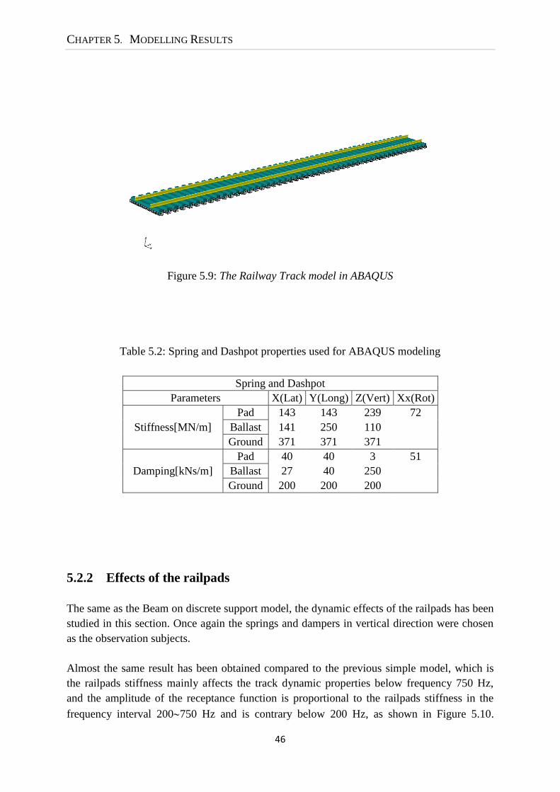
CHAPTER 5. MODELLING RESULTS
46
Figure 5.9: The Railway Track model in ABAQUS
Table 5.2: Spring and Dashpot properties used for ABAQUS modeling
Spring and Dashpot
Parameters X(Lat) Y(Long) Z(Vert) Xx(Rot)
Stiffness[MN/m]
Pad 143 143 239 72
Ballast 141 250 110
Ground 371 371 371
Damping[kNs/m]
Pad 40 40 3 51
Ballast 27 40 250
Ground 200 200 200
5.2.2 Effects of the railpads
The same as the Beam on discrete support model, the dynamic effects of the railpads has been
studied in this section. Once again the springs and dampers in vertical direction were chosen
as the observation subjects.
Almost the same result has been obtained compared to the previous simple model, which is
the railpads stiffness mainly affects the track dynamic properties below frequency 750 Hz,
and the amplitude of the receptance function is proportional to the railpads stiffness in the
frequency interval 200750 Hz and is contrary below 200 Hz, as shown in Figure 5.10.

5.2 DISCRETELY SUPPORTED TRACK INCLUDING BALLAST MASS
47
Figure 5.10: Track receptance function with varying spring stiffness for railpads
As to the effects of the vertical damping of the railpads, the results obtained here also coincide
well with the previous simple model, as shown in Figure 5.11. The railpads damping only
affects the amplitude of the receptance function. The maximum amplitude of the receptance
function increases with the decreasing damping value among frequency range 200Hz to 600
Hz, while has an inverse phenomenon among the frequency range 800 Hz to 1200 Hz. The
same transition point as the previous simple model around frequency 550 Hz has also been
obtained.
Figure 5.11: Track receptance function for track model with varying dashpot for railpads

CHAPTER 5. MODELLING RESULTS
48
5.2.3 Effects of the spring and dashpot of the upper ballast
The receptance functions for different spring stiffness of upper ballast coincide well beyond
frequency 200 Hz as shown in Figure 5.12. Below frequency 200 Hz the resonance frequency
increases with the increasing spring stiffness.
From Figure 5.13 it’s obvious that the viscous damping of the upper ballast mainly affects
frequency below 400 Hz and around 800 Hz. Lower damping value will result in smaller
minimum amplitude of the receptance functions.
Figure 5.12: Receptance curve for track model with varying spring stiffness of upper ballast
Figure 5.13: Receptance curve for track model with varying dashpot of upper ballast

5.2 DISCRETELY SUPPORTED TRACK INCLUDING BALLAST MASS
49
5.2.4 Effects of the spring and dashpot of the under ballast
It has been observed that the spring and dashpot of the under ballast have similar dynamic
effects to the railway track. Both of them mainly affect the frequency below 400 Hz and
frequency around 800 Hz. Around frequency 200 Hz, smaller stiffness and damping value
will result in lower minimum amplitude of the receptance function for both. The results are
shown in Figure 5.14 and Figure 5.15.
Figure 5.14: Receptance curve for track model with varying spring stiffness of under ballast
Figure 5.15: Receptance curve for track model with varying dashpot of under ballast

CHAPTER 5. MODELLING RESULTS
50
5.2.5 Summary of comparison of previous models
After including the ballast and subgrade mass in the Model 2 created in this section, the
dynamic effects of the railpads still manage to coincide well with the previous simple Model 1.
As for the ballast part, since the new model introduced another pair of spring and dashpot
system parallel to the original one, some differences have been observed. For instance, the
ballast spring in Model 1 mainly affects the frequency range below 400 Hz. Similar results
have been obtain only for the under ballast spring in Model 2. While for the upper ballast
spring, it only affects the frequency range below 200 Hz. Another example is about the ballast
dashpot. This time the upper ballast dashpot in Model 2 works the same way as the ballast
dashpot in Model 1.
5.3 Rails on sleepers on continuum
In order to study the dynamic effects of the Trackbed, five models with different trackbed
dimensions were created in ABAQUS. The trackbed contains three layers: Ballast, Subballast
and Subgrade. Solid elements were used for the trackbed simulation. On the ‘infinite
boundaries’, normal displacements were restrained.
In Figure 5.16 and Figure 5.17, the profiles of the cross-section and the boundary conditions
for each model were demonstrated. Model 3, Model 3 (a) and Model 3 (b) have the same
trackbed width 9.3 m but different trackbed shape. As to Model 3 (c) and Model 3 (d), they
share the same trackbed width 21.9 m. The parameters that keep constant are listed in Table
5.3.
Table 5.3: Trackbed components that keep constant
Modulus
(MPa)
Possion's
ratio Density(kN/m3) Thickness(m)
Ballast 150 0.35 16 0.35
Subballast 80 0.35 19 0.15
Subgrade 10 0.4 20 3
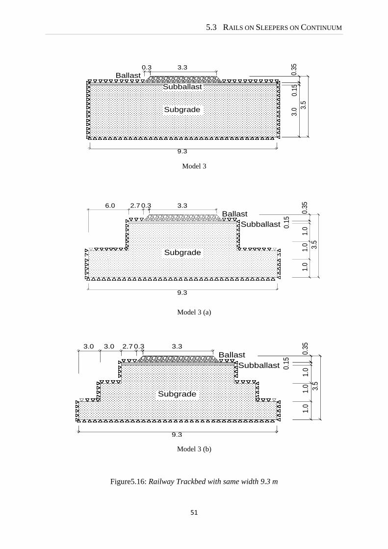
5.3 RAILS ON SLEEPERS ON CONTINUUM
51
3.3
3.5
0.3
50.1
53.0
0.3
9.3
Ballast
Subballast
Subgrade
Model 3
3.30.3
9.3
Ballast
Subballast
Subgrade
3.5
0.3
5
0.1
5
1.0
1.0
1.0
2.76.0
Model 3 (a)
3.30.3
9.3
Ballast
Subballast
Subgrade
3.5
0.3
5
0.1
5
1.0
1.0
1.0
2.73.03.0
Model 3 (b)
Figure5.16: Railway Trackbed with same width 9.3 m

CHAPTER 5. MODELLING RESULTS
52
3.3
3.5
0.3
50.1
53.0
0.3
21.9
Ballast
Subgrade
Subballast
Model 3 (c)
Subballast
Subgrade
3.3
3.5
0.3
5
0.1
5
1.0
0.3
21.9
Ballast
3.03.03.0
1.0
1.0
Model 3 (d)
Figure 5.17: Railway Trackbed with the same width 21.9 m
The Models created in ABAQUS are shown in Figure 5.18 and Figure 5.19 below. The rail
and sleeper parts are the same as Model 1 and Model 2 built earlier. The sleepers are divided
into 10 segments and connected to the ground by spring and dashpot system. For the trackbed,
solid 8 nodes elements were used. Different layers were obtained by the partition of the whole
trackbed and assigning different material properties to each part. The bottom of the trackbed
were constrained in all degrees, while for other ‘infinite boundaries’ only the displacements
normal to the plane were constrained. The trackbed elements that close to the superstructure
of the railway track system are more finely meshed.

5.3 RAILS ON SLEEPERS ON CONTINUUM
53
Model 3
Model 3 (a)
Model 3 (b)
Figure 5.18:Trackbed models that have the same width 9.3m in ABAQUS

CHAPTER 5. MODELLING RESULTS
54
Model 3 (c)
Model 3 (d)
Figure 5.19:Trackbed models that have the same width 21.9 m in ABAQUS
5.3.1 Vibration modes
By the same way as earlier, the Frequency Analysis has been used again in ABAQUS to
extract the eigenmode for railway track system. Some vibration modes for model 3 are
demonstrated in Figure 5.20.

5.3 RAILS ON SLEEPERS ON CONTINUUM
55
f = 1.8844 Hz
f = 2.3574 Hz
f = 3.0821 Hz
Figure 5.20: Some vibration modes of Model 3 extracted from ABAQUS
5.3.2 Effects of the Trackbed Dimension
The results of receptance for all the 5 different models are shown in Figure 5.21. It is obvious
that the size of the trackbed does not affect the dynamic property of the railway track model.
For instance, receptances for Model 3 and Model 3(c), which have the same rectangular shape
but different width 9.3m and 21.3 m respectively, almost overlap each other. The same
happened to Model 3(a), Model 3(b) and Model 3(d). They have the same stepwise shape
trackbed but different trackbed width.

CHAPTER 5. MODELLING RESULTS
56
Figure 5.21:Receptance of railway track with different trackbed models
While the shape of the trackbed has some influences to the receptance curve around frequency
400 Hz. Compared to the receptances for the rectangular shape trackbed, the receptances for
the stepwise shape trackbed have some rightwards movements. The reason for this is maybe
because the imperfect simulations of the boundary conditions for the stepwise shape trackbed.
5.3.3 Effects of the Modulus for each layer
Effect of Ballast Modulus
The ballast modulus is believed to have a major influence on the predicted performances of
the all granular ballast trackbeds, so it is desirable to evaluate the dynamic performance of
trackbeds with varying ballast modulus. Three different ballast moduluses were evaluated.
The modulus was from 150 MPa to 350 MPa, which represents the quality of the ballast from
bad to good. Analytical results are shown in Figure 5.22 for the receptance curve of the
trackbed.
According to Figure 5.22, it can be noted that ballast modulus has a major effect on the
frequency rang below 500 Hz. Lower ballast modulus, which represents soft ballast, fluctuates
more intensively below frequency 200 Hz.

5.3 RAILS ON SLEEPERS ON CONTINUUM
57
Figure 5.22: Track receptance function with varying ballast modulus
Effect of subballast modulus
The same way as for ballast, the effects of subballast modulus has been studied. From Figure
5.23 it’s easy to tell that the subballast modulus mainly affects the frequency range below 400
Hz. The three receptance functions obtained share the same shape, and only some rightwards
movements were discovered for the higher subballast modulus which represents the strong
subballast.
Figure 5.23: Track receptance function with varying subballast modulus

CHAPTER 5. MODELLING RESULTS
58
Effect of subgrade modulus
Besides the ballast and subballast modulus, subgrade modulus is another crucial factor for the
performances of the all granular ballast trackbeds. Evaluation also has been carried out for the
subgrade modulus.
Figure 5.24: Track receptance function with varying subgrade modulus
Once again 3 different subgrade moduluses were evaluated. The modulus was from 10 MPa to
110 MPa, which represent the quality of the subgrade from bad to good. Analytical results are
shown in Figure 5.24 for the receptance curve of the trackbed. It can be noted that subgrade
modulus has a major effect on the frequency rang below 150 Hz. The way the subgrade
affects the receptance function is quite contrary to the ballast modulus, which is the stronger
the subgrade is, the more intensively the receptance function will fluctuate.
5.4 Study of Static Train Load
In order to study the global response of the railway track system due to the passing train load,
a new 3-D model was created in ABAQUS, as shown in Figure 5.25. The model components
are all the same as Model 3 created earlier except the length of the railway track was enlarged
to 200 m.
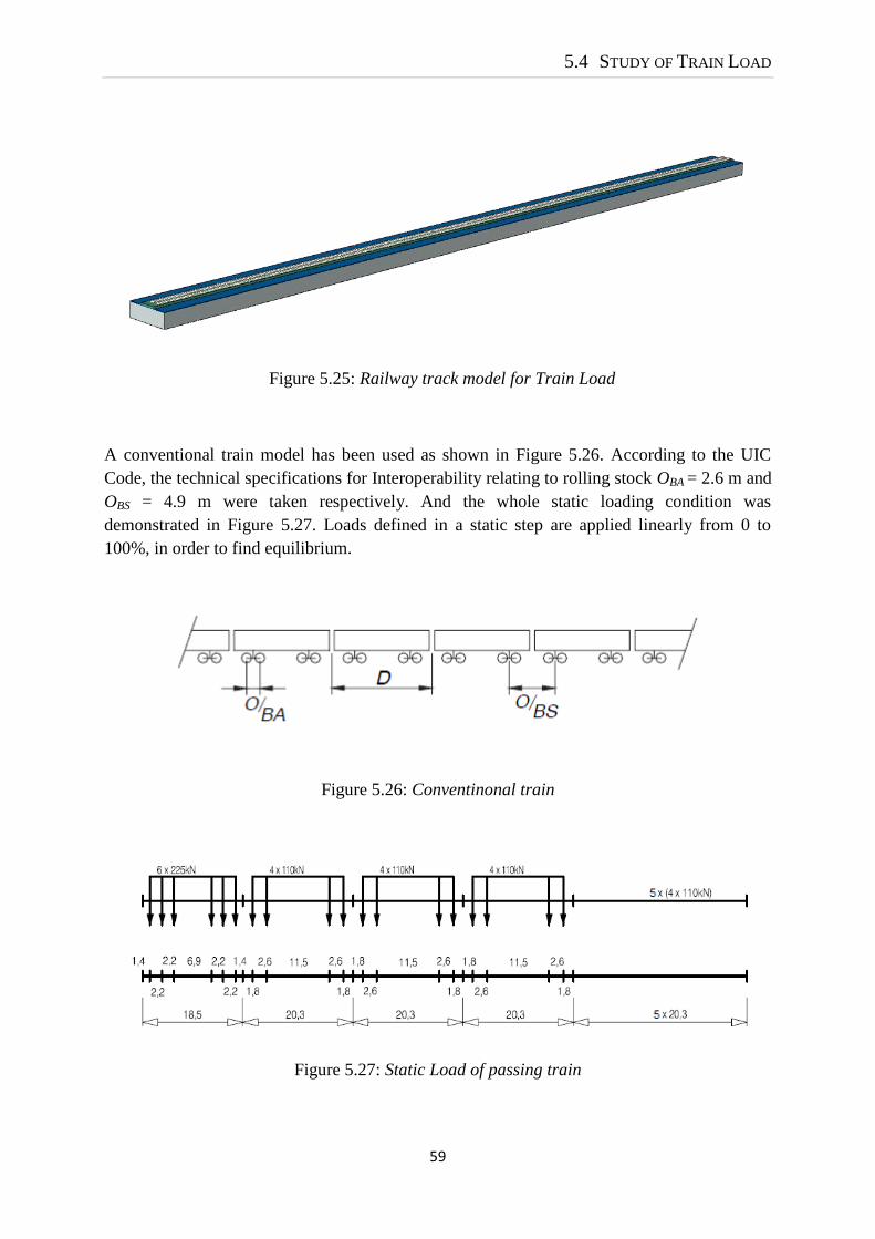
5.4 STUDY OF TRAIN LOAD
59
Figure 5.25: Railway track model for Train Load
A conventional train model has been used as shown in Figure 5.26. According to the UIC
Code, the technical specifications for Interoperability relating to rolling stock OBA = 2.6 m and
OBS = 4.9 m were taken respectively. And the whole static loading condition was
demonstrated in Figure 5.27. Loads defined in a static step are applied linearly from 0 to
100%, in order to find equilibrium.
Figure 5.26: Conventinonal train
Figure 5.27: Static Load of passing train

CHAPTER 5. MODELLING RESULTS
60
Figure 5.28 shows the magnitude of track bed displacement contour, which corresponds well
with the train load distribution. Below the train engine part, the load is bigger and
consequently higher displacements were obtained. While at other parts of the track bed,
almost the same displacement pattern were observed based under the same train load
condition.
A path was created in track bed, which is located 0.35 m under the sleepers and along the
center line of the track bed. The vertical displacement along the path is shown in Figure 5.29.
Figure 5.28: Cut-open view of track bed displacement magnitude contour
Figure 5.29: Track bed displacement along the path

5.4 STUDY OF TRAIN LOAD
61
The vertical strain along the path from ABAQUS was compared to the measurement result
from Magnus Kjörling [20] in Sweden in 1992, as shown in Figure 5.30 and Figure 5.31. It’s
obvious that the patterns from the measurements and FEM modeling match perfectly well.
The vertical stress along the path was also observed from ABAQUS, as shown in Figure 5.32.
Figure 5.30: Strain B2 due to a passenger train from measurement. Speed = 160 km/h
(Measurements on the railroad track at Älgarås, between Laxå and Töreboda, Sweden.
Magnus Kjörling, 1992)
Figure 5.31: Track bed strain due to train load along the path from ABAQUS

CHAPTER 5. MODELLING RESULTS
62
Figure 5.32: Track bed stress due to train load along the path from ABAQUS
5.5 Study of the train speed effect
In order to study the dynamic effect of the train speed to the ground, a much bigger model has
been created this time compared to the models built earlier in this thesis, as shown in Figure
5.33. The railway track components properties remain the same as before. Only the dimension
of the trackbed has been enlarged to 30 m in depth, 30 m in width and 60 m in length
respectively. Here, train load has been modeled as a sequence of constant loads running at a
constant speed over the rails. According to the study of Suiker and De Borst (1999), in
practice the subgrades are usually less stiff than the ballast, and the lowest critical is mainly
determined by the velocity of the train and not influenced by other excitation sources such as
sleeper spacing. On this basis, the assumption of constant moving loads is reasonable for
studying the train speed effect.
The explicit dynamics has been used for calculation. The explicit scheme appeared to be very
computationally demanding and is more appropriate to use when the time interval is very
small. However it is easier to achieve convergence based on an explicit scheme if the
behavior of the structure is unknown.
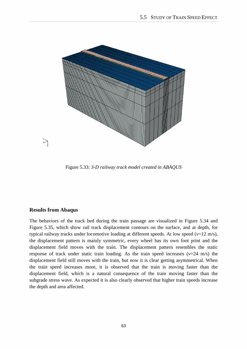
5.5 STUDY OF TRAIN SPEED EFFECT
63
Figure 5.33: 3-D railway track model created in ABAQUS
Results from Abaqus
The behaviors of the track bed during the train passage are visualized in Figure 5.34 and
Figure 5.35, which show rail track displacement contours on the surface, and at depth, for
typical railway tracks under locomotive loading at different speeds. At low speed (v=12 m/s),
the displacement pattern is mainly symmetric, every wheel has its own foot print and the
displacement field moves with the train. The displacement pattern resembles the static
response of track under static train loading. As the train speed increases (v=24 m/s) the
displacement field still moves with the train, but now it is clear getting asymmetrical. When
the train speed increases more, it is observed that the train is moving faster than the
displacement field, which is a natural consequence of the train moving faster than the
subgrade stress wave. As expected it is also clearly observed that higher train speeds increase
the depth and area affected.

CHAPTER 5. MODELLING RESULTS
64
(a) T=0.9 S
Distance along track (m)
(b) T=0.65 S
Distance along track (m)
(c) T=0.31 S
Distance along track (m)
Figure 5.34: Plan views of track displacement response at (a)v=12 m/s, (b)v=24m/s, (c)v=120 m/s

5.5 STUDY OF TRAIN SPEED EFFECT
65
(a) T=0.9 S
Distance along track (m)
(b) T=0.65 S
Distance along track (m)
(c) T=0.31 S
Distance along track (m)
Figure 5.35: At depth views of track displacement response at (a)v=12 m/s, (b)v=24m/s, (c)v=120 m/s

CHAPTER 5. MODELLING RESULTS
66
5.6 Comparison of different Models
5.6.1 The same trackbed stiffness
In this section, according to the complexity three different railway track models created
earlier were compared. They are Model 1: Beam on discrete support model, Model 2: Beam
on discrete support including ballast mass model and Model 3: Rail on sleepers on continuum
respectively. In order to have the same trackbed stiffness, the properties values for each model
built before have been adjusted, as listed in Table 5.4. Only the track properties in vertical
direction have been studied and the value in Table 5.4 is for each sleeper segment.
Figure 5.36: Cut-open view of trackbed displacements along loading plane in lateral(u1),
longitudinal(u2) and vertical(u3) direction under 1 unit load on the rails in ABAQUS

5.6 COMPARISON OF DIFFERENT MODELS
67
The approach for reaching the same trackbed stiffness is by applying 1 unit concentrated force
on the middle point of the rail between two sleepers, and then carrying out a static analysis to
get the displacement for the corresponding point. Therefore, the trackbed stiffness k will be
1/. In this study case the trackbed stiffness k=1*108 N/m has been used as the standard.
Figure 5.36 shows Cut-open view of trackbed displacements along loading plane in lateral(u1),
longitudinal(u2) and vertical(u3) direction under 1 unit load on the rails in ABAQUS.
Table 5.4. Properties of railway track
Symbol Value Description
Model 1
Krs 239 MN/m Railpad stiffness
Crs 500 kNs/m Railpad viscous damping
Kbg 15 MN/m Ballast stiffness
Cbg 50 kNs/m Ballast viscous damping
Model 2
Krs 239 MN/m Railpad stiffness
Crs 500 kNs/m Railpad viscous damping
Ksb 26.5 MN/m Upper ballast stiffness
Csb 100 kNs/m Upper ballast damping
Kbg 35 MN/m Under ballast stiffness
Cbg 50 kNs/m Under ballast damping
Model 3
Krs 239 MN/m Railpad stiffness
Crs 500 kNs/m Railpad viscous damping
Ksg 1.1 MN/m Stiffness between rail and trackbed
Csg 50 kNs/m Damping between rail and trackbed
Eb 200 Mpa Ballast Modulus
Esubb 100 Mpa Subballast Modulus
Esubg 30 Mpa Subgrade Modulus
*The stiffness and damping values are all for vertical direction
**Except the values for the railpad, all the other stiffness and damping value is for per
segment along the sleeper and the ground.
5.6.2 Comparison of CPU time for eigenvalue analysis
The CPU time for different eigenvalue analysis, performed with the Lanczos eigen-solver in
the interval of 0 to 30 Hz, are presented in Table 5.5. It is seen that the CPU time for the
analysis is rather small. Even if a very detailed solid model is used the CPU time is not longer

CHAPTER 5. MODELLING RESULTS
68
than 3 minutes. The analysis has been performed with a Intel Core 2 Duo Processor T6400
(2.0GHz) with 4 GB of random access memory (RAM).
Table 5.5: Acquired CPU time for the eigenvalue analysis
Eigenvalue Analysis
Model DOF NO. Of Modes CPU Time (s)
Model 1 7812 6 2.7
Model 2 10612 6 17.4
Model 3 26828 62 50.2
5.6.3 Comparison of receptance curve
Figure 5.37: Comparison of receptance functions for three railway track model
The differences of three railway track models are clearly illustrated in a comparison of
corresponding receptance function for each model in Figure 5.37. It’s obvious that Model
1coincides well with Model 2, for which both simulating the trackbed by spring and viscous
damper system. However, compared to the first two models, significant differences have been
observed for Model 3, which has used different layers of solid element for the simulation of
trackbed. The main differences are:

5.6 COMPARISON OF DIFFERENT MODELS
69
Solid element model generally has lower receptance amplitude compared to spring and
viscous damper models. The largest difference happened around frequency 1000 Hz,
and the corresponding receptance amplitude are 10.15*10-9
m/N and 2.28 *10-9
m/N
respectively. The difference is almost 77%.
The resonance frequency around 1000 Hz obtained from solid element model is higher
than the one got from the spring and viscous damper model, which are 1028 Hz and
927 Hz respectively.
There is one obvious fluctuation around frequency 1100 Hz for spring and viscous
damper model, however this cannot be observed from solid element model around that
frequency range. All the other parts of the three models almost share the same trend.
5.6.4 Comparison of beam element model and solid element model
With the intention of obtaining more accurate results, solid element was used for the
simulation of the rails and sleepers. The solid element model is more detailed than the beam
element model. The size of the mesh is not a problem when dealing with static analysis, as
long as the mesh is not too coarse. When using dynamic analysis though, it radically increases
the computational cost, because the time increment is based on the smallest element in the
model. Figure 5.38 shows the mesh of the rail in the new model.
Figure 5.38: Solid element for the rail

CHAPTER 5. MODELLING RESULTS
70
Figure 5.39: Model of solid element for rails and sleepers with sleepers embedded in ballast
Based on Model 3 two more models were created. For the first model only the rail part was
replaced by solid element. While for the second model, both the rail and sleeper parts were
generated by solid element. Besides, the sleepers were embedded in the ballast layer. As
shown in Figure 5.39.
Figure 5.40: Comparisons of receptance between beam element and solid element

5.6 COMPARISON OF DIFFERENT MODELS
71
The results of receptance functions obtained from the solid element model are compared to
the one from Model 3, which uses beam element for the rails and sleepers. In Figure 5.40, the
curve of ‘Solid element’ is for the first model with only the replacement of the rail part by
solid element, and ‘Solid element*’ is for the second model which uses solid element for both
the rail and sleeper.
It is obvious all the three models have the same trend before 600 Hz, especially the peak
around 400 Hz. After frequency 500 Hz, the receptance function for solid element become
significantly undulate. The reason for this might be due to the deformation of the solid rail
profile, which has not been taken into account for the beam element. Another obvious
difference is that the pin-pin resonance around 1000 Hz is missing for the solid element
models. The reason for this is complicated and deserves further research.

72

73
Chapter 6
Conclusions and suggestions for
future work
The purpose of this thesis was to study the dynamic effects of railway track components based
on three dimensional finite element methods. Considering the complexity, different models
were created and compared. Conclusions about the method and results are presented below.
Suggestions for future study also have been proposed.
6.1 Conclusions The railway track structure always starts to vibrate in lateral direction, following the
vibration way of rails as simply supported beam. Depending on the connection
conditions between the track components, after reach certain frequency the vertical
vibration modes get the domination. More vibration modes were extracted from the
solid trackbed model.
Comparatively speaking, the spring and dashpot in vertical direction have more
significant effects on dynamic properties of the railway track system compared to
other directions. The stiffness of the railpads have a major effects on the resonance
frequency, while the damping of the dashpot mainly influences the amplitude of the
receptance curve. The properties of the trackbed multilayer mainly affect the
receptance function below 400 Hz.

CHAPTER 6. CONCLUSIONS AND SUGGESTIONS FOR FUTURE WORK
74
As long as the same boundary conditions were applied, the size of the solid trackbed
doesn’t affect the dynamic properties of the railway track at all. On the other hand, the
shape of the solid trackbed will influence the resonance frequency.
The speed of the moving train has a significant dynamic effect on the trackbed. As the
train speed increases, the displacement pattern of trackbed changes from symmetrical
to asymmetrical.
6.2 Further research
Instead of using spring and dashpot, different contact method could be considered for
the connection between the sleeper and trackbed. For instance, it could be modeled as
sleepers embedded in the trackbed, which is more close to reality.
The critical speed should be taken into account when study the speed effect of the train.
Correspondingly more comprehensive model should be built. For instance, energy
absorbing boundaries should be used to avoid any possible fictitious ground wave
reflections.
There exist an obvious difference between the beam element model and solid element
model regarding to the receptance function. The reason for this deserves more study.
In order to be convenient to operate, more user friendly interface could be developed
by using programming software like Matlab.

75
Bibliography
[1] ABAQUS Online Documentation: Version 6.9 (2011).
http://abqdoc.byv.kth.se:2011/v6.9/
[2] COENRAAD ESVELD. Modern Railway Track, Second Edition. Delft University of
Technology. 2001.
[3] TORE DAHLBERG. Railway track dynamic – a survey. Solid mechanics/IKP,
Linköping University. 2003.
[4] M P N BURROW1
, D BOWNESS2
, and G S GHATAORA3
. A Comparison of railway
Track foundation design methods.1,3
Dep. of civil Engineering, The University of
Birmingham, Birmingham, UK. 2School of Civil Engineering and the environment,
University of Southampton, Southampton, UK. 2006.
[5] J.T.SHAHU, AMIT SHARMA AND K.G.SHARMA. Numerical Modelling of Railway
Tracks with Ballast and Subballast Layers using Critical State Parameters. Dep. of Civil
Engineering, Indian Institute of Technology Delhi, Delhi, India. 2008.
[6] AMNON PIETER DE MAN. Dynatrack – A Survey of Dynamic Railway Track
Properties and their Quality. Delft University of Technology, Delft, the Netherlands.
2002.
[7] Z. CAI1 AND G.P. RAYMOND
2. Modelling the dynamic response of railway track to
wheel/rail impact loading.1Dep. of Civil Engineering, Royal Military College, Kingston,
Ontario, Canada. 2Dep. of Civil Engineering, Queen’s University, Kingston, Ontario,
Canada.1994.
[8] AHLBECK D.R, MEACHAM H.C. AND PRAUSE R.H. The development of
analytical models for railroad track dynamics. Oxford. 1975.
[9] A.P.DE MAN. Pin-pin resonance as a reference in determining ballasted railway track
vibration behavior. Railway Engineering Group, Faculty of Civil Engineering and
Geosciences, Delft University of Technology.2000.
[10] KENNEY, J.T. Steady-state vibrations of beam on elastic foundation for moving load.
Journal of applied Mechanics. 1954.
[11] KJELL ARNE SKOGLUND. A Study of Some Factors in Mechanistic Railway Track
Design. Norwegian University of Science and Technology. 2002.

76
[12] M.BANIMAHD1 AND P.K.WOODWARD
1&2. Numerical Study of Train Speed Effect
on Railway Track Response. 1School of the Built Environment, Heriot Watt University,
Edinburgh.2XiTRACK Limited, Station Road, Birch Vale, High-Peak,Derbyshire.2007.
[13] OSCARSSON J. Dynamic train-track interaction: linear and non-linear track models
with property scatter. PhD Thesis. Department of Solid Mechanics, Chalmers
University of Technology, Gothenburg, Sweden. 2001.
[14] CHANG CS, ADEGOKE CW,SELIG ET. GEOTRACK model for railroad track
Performance. Journal of Geotechnical Engineering Division. 1980;ASCE, 106(GT11):
1201-1218.
[15] LOUIS LE PEN. Track Behaviour: The Importance of the Sleeper to Ballast Interface.
PhD Thesis. School of Civil Engineering and the Environment,University of
Southampton. 2008.
[16] MOHAMED A. SHAHIN. Investigation into some design aspects of ballasted railway
Track structure. Dep. of Civil Engineering, Curtin University of Technology, Perth,
WA 6845, Australia. 2008.
[17] MINGFEI LU. Discrete Element Modelling of Railway Ballast. PhD Thesis. The
University of Nottingham. 2008.
[18] ERNEST T. SELING AND JOHN M. WATERS. Track geotechnology and
substructure management. T. Telford, American Society of Civil Engineers. 1994.
[19] ANDREAS ANDERSSON AND RICHARD MALM. Measurment evaluation and
FEM simulation of bridge dynamic. Royal Institute of Technology, Sweden, 2004.
[20] MAGNUS KJÖRLING. Dynamic response of railway track components –
Measurements during train passage and dynamic laboratory loading. Department of
Structural Engineering. Royal Institute of Technology, Sweden.

77
Appendix A
ABAQUS input file data for Model 3
*Part, name=MULTILAYERS
*Element, type=C3D8R
** Section: Section-1-_PICKEDSET17
*Solid Section, elset=_PICKEDSET17, material=SUBGRADE
,
** Section: Ballast
*Solid Section, elset=_PickedSet6, material=BALLAST
,
** Section: Section-2-_PICKEDSET16
*Solid Section, elset=_PICKEDSET16, material=SUBBALLAST
,
*End Part
**
*Part, name=RAIL
*Element, type=B31
** Section: Section-3-_PICKEDSET2 Profile: Profile-1
*Beam Section, elset=_PICKEDSET2, material=STEEL, temperature=GRADIENTS, section=I
0.084, 0.159, 0.14, 0.07, 0.0145, 0.0363, 0.016
-1.,0.,0.
*End Part
**
*Part, name=SLEEPER
*Element, type=B31
** Section: Section-4-_PICKEDSET2 Profile: Profile-2
*Beam Section, elset=_PICKEDSET2, material=CONCRETE, temperature=GRADIENTS, section=RECT
0.3, 0.2
0.,1.,0.
*End Part
**
**
** ASSEMBLY
**
*Assembly, name=Assembly
**
*Instance, name=MULTILAYERS-1, part=MULTILAYERS
*End Instance
**
*Instance, name=RAIL-1, part=RAIL
*End Instance
**
*Instance, name=SLEEPER-1, part=SLEEPER
*End Instance
**
*Nset, nset=Middle, instance=RAIL-1
*Element, type=Spring2, elset=RSX-spring
*Element, type=Dashpot2, elset=RSX-dashpot
*Spring, elset=RSX-spring
1, 1
1.43e+08

78
*Dashpot, elset=RSX-dashpot
1, 1
40000.
*Element, type=Spring2, elset=RSXx-spring
*Element, type=Dashpot2, elset=RSXx-dashpot
*Spring, elset=RSXx-spring
4, 4
7.2e+07
*Dashpot, elset=RSXx-dashpot
4, 4
51000.
*Element, type=Spring2, elset=RSY-spring
*Element, type=Dashpot2, elset=RSY-dashpot
*Spring, elset=RSY-spring
2, 2
1.43e+08
*Dashpot, elset=RSY-dashpot
2, 2
40000.
*Element, type=SpringA, elset=RSZ-spring
*Element, type=DashpotA, elset=RSZ-dashpot
*Spring, elset=RSZ-spring
2.39e+08
*Dashpot, elset=RSZ-dashpot
3000.
*Element, type=Spring2, elset=SGX-spring
*Element, type=Dashpot2, elset=SGX-dashpot
*Spring, elset=SGX-spring
1, 1
1.41e+08
*Dashpot, elset=SGX-dashpot
1, 1
27000.
*Element, type=Spring2, elset=SGY-spring
*Element, type=Dashpot2, elset=SGY-dashpot
*Spring, elset=SGY-spring
2, 2
2.5e+08
*Dashpot, elset=SGY-dashpot
2, 2
40000.
*Element, type=SpringA, elset=SGZ-spring
*Element, type=DashpotA, elset=SGZ-dashpot
*Spring, elset=SGZ-spring
1.1e+08
*Dashpot, elset=SGZ-dashpot
250000.
*Element, type=Spring1, elset=SLeeperX-spring
*Spring, elset=SLeeperX-spring
1
1e+09
*Element, type=Spring1, elset=SLeeperY-spring
*Spring, elset=SLeeperY-spring
2
1e+09
*Element, type=Spring1, elset=SLeeperZ-spring
*Spring, elset=SLeeperZ-spring

79
3
1e+09
*End Assembly
**
** MATERIALS
**
*Material, name=BALLAST
*Density
1600.,
*Elastic
1.5e+08, 0.35
*Material, name=CONCRETE
*Density
2400.,
*Elastic
7e+10, 0.3
*Material, name=STEEL
*Density
7850.,
*Elastic
2.1e+11, 0.3
*Material, name=SUBBALLAST
*Density
1900.,
*Elastic
8e+07, 0.35
*Material, name=SUBGRADE
*Density
2000.,
*Elastic
1e+07, 0.4
**
** BOUNDARY CONDITIONS
**
** Name: RailFixed Type: Symmetry/Antisymmetry/Encastre
*Boundary
_PickedSet4786, ENCASTRE
** ----------------------------------------------------------------
**
** STEP: Step-1
**
*Step, name=Step-1, perturbation
*Steady State Dynamics, direct, frequency scale=LINEAR, friction damping=NO
0., 1300., 130, 1.
**
** BOUNDARY CONDITIONS
**
** Name: BedBottom Type: Symmetry/Antisymmetry/Encastre
*Boundary
_PickedSet4781, ENCASTRE
** Name: BedX Type: Displacement/Rotation
*Boundary, load case=1
_PickedSet4782, 1, 1
*Boundary, load case=2
_PickedSet4782, 1, 1
** Name: BedY Type: Displacement/Rotation
*Boundary, load case=1

80
_PickedSet4783, 2, 2
*Boundary, load case=2
_PickedSet4783, 2, 2
** Name: BedY2 Type: Displacement/Rotation
*Boundary, load case=1
_PickedSet4784, 2, 2
*Boundary, load case=2
_PickedSet4784, 2, 2
**
** LOADS
**
** Name: Load-1 Type: Concentrated force
*Cload, load case=1
_PickedSet4780, 3, 1.
**
** OUTPUT REQUESTS
**
**
** FIELD OUTPUT: F-Output-1
**
*Output, field, variable=PRESELECT
**
** HISTORY OUTPUT: H-Output-1
**
*Output, history, variable=PRESELECT
*Node Print, NSET=Middle, SUMMARY=NO
PU3
*End Step