LARGE-SCALE MASS TRANSPORT MODELLING IN DISCRETELY-FRACTURED POROUS MEDIA

Guillaume Kenny, Département de géologie et de génie géologique, Université Laval, Québec

René Therrien, Département de géologie et de génie géologique, Université Laval, Québec André Fortin, Groupe interdisciplinaire de recherche en éléments finis, Université Laval, Québec

Cristian Tibirna, Groupe interdisciplinaire de recherche en éléments finis, Université Laval, Québec

ABSTRACT A numerical model has been developed for the large-scale simulation of solute transport in discretely-fractured porous media. A generic finite elements code, MEF++, has been used to account for simultaneous flow and transport in 2D fracture and 3D porous medium elements. Equations for the fractures and the porous medium are solve separately but are coupled with a mass transfer term. This mass transfer term is calculated using the concentration gradient and weighted with a coefficient that depends on the porous medium properties, allowing for a general representation of diffusive exchange between fracture and porous medium. Verification and illustrative examples are presented to illustrate the modeling capabilities, including adaptive meshing for the transport solution. RÉSUMÉ Un modèle numérique a été développé pour la simulation à grande échelle du transport de masse dans un milieu poreux à fracturation discrète. Un code d’éléments finis générique, MEF++, a été modifié pour inclure l’écoulement de l’eau et le transport de masse dans des éléments de fractures 2D et des éléments 3D pour la matrice poreuse. Le modèle résout séparément les équations pour les fractures et pour la matrice poreuse, avec couplage par un terme de transfert de masse. Ce terme de transfert est calculé à partir du gradient de concentration entre le milieu poreux et la fracture et il est pondéré par un coefficient dépendant des propriétés du milieu poreux. Cette approche permet une représentation générale du transfert entre fractures et matrice. Des exemples sont présentés pour vérifier le modèle et pour illustrer ses capacités, particulièrement l’adaptation de maillage qui permet d’améliorer les résultats des simulations.

848

1. Introduction Groundwater availability plays a key role in the development of populations, but population growth affects its quality. In several countries, environmental laws are getting more strict to minimize the impact of human activities on groundwater quality. Mathematical models that describe groundwater flow and solute transport, based on analytical or numerical solutions to the governing equations, are becoming increasingly used for groundwater management. Because of the method of solution used, analytical models are generally restricted to simple homogeneous groundwater systems. For complex geological environments, their applicability can become limited and numerical models often become the best option. Fractured geological materials, where complex fractures networks can exist, represent one example of such complex environments. Several conceptual models exist to represent groundwater flow and solute transport in fractured geological systems. The most commonly used are the equivalent porous medium (EPM) model, the dual-continuum model and the discrete fracture model. The differences between each model reside in their mathematical complexity, data requirement and also on their ability to accurately represent observations. The EPM approach treats the porous medium and fractures as a single domain, with a single set of hydraulic and transport properties. For large-scale domains, this approach can be inaccurate because it relies on the existence of a representative elementary volume (REV) for the equivalent medium. Such generalization of the domain may fail in complex fracture networks where discrete flow paths, or channels, exist. The second approach is the dual-continuum model. In this approach, the porous medium and fractures form two separate domains that are both represented by their own REV. In the mathematical formulation, both domains are coupled with a fluid or mass exchange term. For large-scale domains, this approach can also be inaccurate if discrete fractures are present in the porous medium. The third conceptual model is based on a discrete representation of individual fractures. Each fracture is located in the simulation domain and assigned hydraulic and transport properties. The model FRAC3DVS, presented by Therrien and Sudicky (1996), is an example of a 3D discrete fracture numerical model for fluid flow and solute transport. The model solves the flow and transport equation with the control volume finite element method. Fractures are represented by 2D planar elements and the porous medium is represented by 3D volumetric elements. Because fractures are discretized in two dimensions, it is assumed that solute and head distributions across the fracture aperture are uniform. This assumption is reasonable for large-scale simulations since solute and hydraulic head distributions across a fracture will likely be irregular only at very small scales. Another assumption is that a fracture is idealized as uniform parallel plates. The 2D fracture elements are superposed onto the 3D porous medium elements and continuity of hydraulic head and solute concentration is assumed at nodes that are common to fracture and porous medium. This representation of the system helps reduce the numerical and meshing difficulties arising from the large contrast between fracture aperture and total domain size. As opposed to the EPM or dual-continuum approaches, the discrete fracture approach can be considered as that requiring the most detailed field knowledge, but it can also provide the most realistic representation of the fractured rock mass. However, some difficulties still exist for the application of discrete fracture model. The first difficulty is to characterize the rock mass including individual fractures and to derive hydraulic and transport properties for input into the model. A second difficulty is related to the discretization and numerical solution of the flow and transport equations for large-scale simulations. There is a very strong contrast between a typical fracture aperture, which is often less than 1 mm, and flow and transport distances of interest for practical applications, which can exceed hundreds of meters. As a result, for large spatial domains, discretization problems might arise because of the large thickness ratio between the fracture and the porous medium. Furthermore, an accurate description of fluid flow and transport processes close to the fracture wall, into the porous medium, might require very fine grids, making the numerical solution computationally very expensive. This paper presents preliminary results concerning the development of a model for mass transport and saturated groundwater flow over large distances in discretely-fractured porous media. The model presented here has been developed using a flexible multi-purpose finite element code (MEF++) that allows adaptive mesh refinement (Fortin, 2004). It is based on the approach used in FRAC3DVS where fractures are discretized with 2D elements and the porous medium is discretized with 3D elements. Equations of groundwater flow (diffusion) and mass transport (diffusion and advection) for both fractures and porous medium are coupled to produce the numerical model. The purpose of the work is to improve the current

849

conceptual model capabilities for fractured rock simulations and address the numerical difficulties mentioned above. A major difference between this model and FRAC3DVS is the computation of mass transfer between the fracture and the porous medium. A mass transfer coefficient that depends on the porous medium properties is introduced in the transport equation for both transport media, rather than assuming continuity of concentration at the fracture and the porous medium interface. This mass transfer coefficient weighs the existing concentration gradient between the fracture and the porous medium. The value of this coefficient is found by comparison and adjustment with experimental data. In addition to this coefficient, adaptive mesh refinement is used during the simulation to account for the slow process of mass diffusion in the porous medium and also for the high concentration gradient that can occur in the system. This last feature of the model, coupled with a more general representation of mass transfer, allow to model accurately mass transport over large distance in fractured rock. In the following sections of this paper, governing equations used to build the model and their numerical implementations are presented. The model is compared to an analytical solution for solute transport in a network of parallel fractures (Sudicky and Frind, 1982). Illustrative simulations are then presented for large-scale transport in fractured rock, for a system that resembles that in Smithville, Ontario, where a fractured carbonate aquifer has been contaminated by PCB (Novakowski et al., 1997). 2. Governing equations The fluid flow and mass transport equations used to build the numerical model for the porous medium and the fracture are presented in this section. Their numerical implementation, associated boundary conditions and mass coupling terms are presented in section 3. 2.1 Porous medium 2.1.1 Fluid flow The following equation is used to describe three-dimensional transient groundwater flow in a saturated porous medium:

[1] where is the Darcy velocity [L T ], the hydraulic head [L] and 1-

rh rK the hydraulic conductivity of the porous medium [L T - ]. The volumetric fluid flux Q [L 3 L - T - ] represents sources (positive) or sinks (negative) for fluid flow in the porous medium. The right-hand side of the equation represents fluid storage, with

1hr

3 1

srS being the specific storage coefficient of the porous medium [L - ]. 1

2.1.2 Mass transport The following equation describes three-dimensional mass transport in a saturated porous medium:

[2] where is the solute concentration in the porous medium [M L - ], θ is the porous medium porosity [dimensionless], Q represents a sink (negative) or a source (positive) that allows solute exchange with the outside of the porous medium [M L - T - ] and R is a dimensionless retardation factor given by (Freeze and Cherry, 1979):

rC 3

Cr3 1

r

850

[3] where ρb is the bulk density of the porous medium [M L ] and 3-

drK is the water-solid distribution coefficient for the porous medium [L M - ]. The retardation factor accounts for the slower migration of a solute, compared to water, because of adsorption onto the porous medium (Charbeneau, 2000). The diffusion coefficient of the porous medium is defined by [L T - ] (Bear, 1972):

3 1

rD 2 1

[4] where is the free-solution diffusion coefficient [L T - ] and τ is the porous medium tortuosity [dimensionless].

D* 2 1

In equation 2, the advection term is omitted since the porous medium is assumed to have a very low-permeability. As a result, the effect of advection is negligible relative to the diffusion term for the porous medium. Omitting advection is done to simplify the model description but, since the numerical model (MEF++) is designed to solve several types of partial differential equations, advection can be included in equation 2 with very few modifications. 2.2 Fracture 2.2.1 Fluid flow The following equation describes three-dimensional transient groundwater flow in a saturated fracture:

[5]

where is the Darcy velocity [L T ], 1-fh is the hydraulic head [L] and Q correspond to

a volumetric fluid flux corresponding to a source (positive) or sink (negative) for the fracture [L L - T - ]. The right-hand side of the equation represents fluid storage in the fracture, with

hf3 3

1sfS2

being the

specific storage coefficient [L ] that is directly related to the water compressibility, α1-w [L T M - ]. The

saturated hydraulic conductivity of a fracture 1

fK having a uniform aperture 2 [L] is given by (Bear, 1972):

b

[6] where is the density of water [M L ], g is gravitational acceleration [L T ] and µ is the viscosity of water [M L T - ].

wr 3- 2-

1- 1

2.2.2 Mass transport Three-dimensional mass transport in a saturated fracture is described by:

[7] where fC is the solute concentration in the fracture [M L - ], Q is a solute source or sink in the fracture

[M L T ] and

3Cf

3- 1-fD is the fracture diffusion coefficient defined by [L 2 T - ]: 1

[8]

851

where D is the free solution dispersion coefficient and α*L is the longitudinal dispersivity. The

dimensionless retardation factor, fR , is defined as (Freeze and Cherry, 1979):

1 dff

KR

b= + [9]

where dfK is the water-solid distribution coefficient of the fracture [L]. 3. Numerical Implementation 3.1. Discretized equations Discretized form of the saturated fluid flow and mass transport equations are presented in this section for both simulation domains. The coupling method is also presented in detail. 3.1.1 Porous Medium Governing equation 1 describing fluid flow in the porous medium can be rewritten as:

[10] where Ψfr is a fluid exchange term at the fracture/ porous medium interface. The equation of mass transport can also be rewritten in a similar fashion:

[11] where Γfr is a mass exchange term at the fracture/ porous medium interface. The variational form of equations 10 and 11 are obtained by integration by part of their left-hand side and had the following form:

[12] and:

[13] where are the tests functions used in the Galerkin variational method and is normal to the boundary. rv n Equations 12 and 13 represent essentially the same transient diffusion phenomenon but with different coefficients. The first represents mass accumulation while the second represents diffusion. Both terms are integrated over the volume of the porous medium. The third term, also a diffusion term, is integrated over the boundaries (surfaces) of the porous medium domain and represents a transfer of mass between the porous medium and the exterior of its domain. Other models (for example, Therrien and Sudicky (1996)) that assume continuity of concentration at the fracture and porous medium interface omit this boundary diffusion. As results, these models assume instantaneous exchange between the porous medium and the fracture. If it is assume that the boundary integral represents transfer between the fracture and the porous medium, it is possible to write for the fluid flow:

[14] and for the mass transport:

852

[15] where hH is the fluid flow transfer coefficient [T - ] and H1

m is the mass transfer coefficient [T - ]. The right-hand side term of these equations can be viewed as the exchange term Ψ

1

fr in equation 10 and Γfr in equation 11. Replacing equations 14 and 15 in equations 12 and 13 respectively, the following variational form of the fluid flow and mass transport equations in the porous medium are obtained:

[16] and:

[17] As an example, inspection of equation 17 indicates that, if the concentration in the porous medium is equal to that in the fracture, there is no mass transfer between both systems. However, if fC is greater thanC , the right-hand side is positive and there is transfer of mass from the fracture towards the porous medium.

r

3.1.2 Fracture The equation for fluid flow in a fracture (equation 5) can be rewritten as:

[18] and in the same way, the mass transport equation 7:

[19] where Ψrf is a fluid exchange term and Γrf is a mass exchange term at the fracture/porous medium interface. Using integration by part, the variational form of equations 18 and 19 can be written as:

[20] and:

[21] where fv are test functions used in the variational method of Galerkin and n is normal to the boundary. We make the assumption that solute concentration is uniform across the fracture aperture to reduce the dimensionality of the equation. We further assume that a fracture can be represented as parallel plates. From these assumptions, the volume integrals in equation 20 and 21 are reduced to surface integrals when integrating these over the fracture aperture2 , such that: b

[22] and

853

[23] In these last two equations, the boundary diffusion term represents a transfer of mass between the fracture and the porous medium and so they can be written as follow:

[24] and

[25] where the right-hand side of equations 24 and 25 are equivalent to Ψrf in equation 18 and Γrf in equation 19 respectively. Replacing equation 24 in equation 22, the following variational form of the fluid flow equation in the fracture is obtained:

[26] In the same way, using equation 25 in equation 23, the following variationnal form of mass transport equation is obtained:

[27] These final equations show that the fracture is reduced to a two-dimensional surface that can be coupled with the three-dimensional porous medium equations 16 and 17 using the boundary exchange term that appears in both equations. 3.2 Numerical techniques To discretize the governing equations, a standard Galerkin formulation is used with piecewise linear approximation of the primary variables. Special care must be taken regarding numerical problems that occur when simulating mass transport in discretely-fractured rock. First, the advection term in equation 7 is usually much larger than the diffusion term. It produces advection-dominated transport in the fracture, for which the standard Galerkin method can produce numerical oscillation. Therefore, a Streamline Upwind Petrov Galerkin (SUPG) scheme (Bourisli, 2002) is used in the fractures to eliminate oscillations introduced by the convection term. This scheme consists in replacing the test function fv by vf + cqf ⋅ vf , where c is a coefficient depending on the element size. This is the finite element equivalent of the backward finite differences used in highly convective cases. The second numerical difficulty is related to discretization of the fracture, namely the strong contrast between the fracture aperture and transport distances for practical applications, as well as potentially strong concentration gradients between the fracture and surrounding porous medium. As shown in section 3.1.2, the flow and transport equations are averaged over the fracture thickness and both processes are therefore represented in two dimensions, which do not require discretization across the fracture thickness. Strong concentrations gradients occur when a moving solute front in the fracture is in contact with an uncontaminated portion of the porous medium. In that case, there is an abrupt change of concentration over a very short distance, across the fracture/porous medium interface. There is also an abrupt change in the solute transport velocity, since there is fast advective transport in the fracture and slow diffusive transport in the porous medium. To capture these strong concentration gradients without having to use an extremely fine

854

mesh over the whole domain, thus improving the accuracy of the simulations, an adaptive remeshing strategy is introduced based on an error estimator. It allows to refine the mesh where needed while coarsening the mesh in other regions. This strategy will not be described here but the reader is referred to the following references for a complete discussion (see Belhamadia et al. (2004a, b)). 3.2 Computer implementation In order to verify the conceptual model, MEF++, a general purpose finite element model, has been used. MEF++ is a sophisticated object-oriented implementation of a large number of aspects of the finite element method. With its object-oriented implementation, MEF++ allows to build the model for a given partial differential equation for more or less generic building blocks called formulation terms. These formulation terms are assigned to a global container object, to form a whole problem. This global object also contains information about the mesh, the boundary and initial conditions, the pre- and post-treatments and the solver to use in order to simulate the behavior of the partial differential equation. Five formulation terms (1 advection term, 1 diffusion term, 1 source term and 2 mass terms) are used to solve equation 27. To reproduce the behavior of the conceptual model presented in this paper, two global container objects are used, one for the fracture system and one for the porous medium system. They are coupled using the source and mass terms that appear on the right-hand side of both equations (see equations 26 and 27). The coupling between the two containers is done using a non-linear iterative solver. An arbitrary tolerance (very low numerically) is used for the convergence of this solver. An adaptive time stepping algorithm has also been used to increase the efficiency and accuracy of the numerical model. The algorithm is similar to that used in FRAC3DVS, where the maximum concentration change between two time steps is controlling the size of the time step. A pre-treatment is done using GMSH (2004) an automatic 3D finite element grid generator, which is used to build the finite element mesh of the simulation domain. The mesh created is imported in iMEF++, a graphical interface to MEF++ where domain boundary and initial conditions, hydraulic parameters and geometries such as fractures and hydraulically different porous medium are defined by the user. Then iMEF++ creates the set of files that are used by MEF++ to run the simulation. The post-treatment is done by exporting plain data such as concentration profiles or breakthrough curves or by viewing the results using VU (2004), a configurable visualization software tool for the display and analysis of numerical solutions. 4. Verification The model has been verified by first performing some numerical tests to ensure that the governing equation is correctly solved, and then by comparing to a published analytical solution for solute transport in a set of parallel fractures embedded into a porous medium. 4.1 Numerical testing Numerical testing can be conducted within MEF++ to ensure that the discretized equation is correctly solved. The procedure does not require that an analytical solution be available for the equation. Instead, the procedure consists in assuming an arbitrary solution to the discretized equations, for example the concentration at all nodes for equation 16, and then solve analytically outside of MEF++ to determine the boundary conditions necessary to produce the arbitrary solution. Verification of the model is then conducted by specifying these boundary conditions within MEF++ and then computing the unknown solution at the nodes. The model should reproduce the same solution as used to determine the boundary conditions. Using this method, extensive testing of the numerical model has been done and showed that the governing equations are indeed correctly solved. Using several different analytical expressions, simulations have also indicated excellent mass conservation for the model. 4.2 Analytical solution Sudicky and Frind (1982) have developed an exact analytical solution for transient solute transport in discrete parallel fractures situated in a porous medium. The solution takes into account advective transport

855

in the fracture, molecular diffusion and mechanical dispersion along the fracture axes, molecular diffusion from the fracture to the porous medium, adsorption and radioactive decay. A transient solution has also been developed for the case where longitudinal dispersion is omitted when advective flux in the fracture is large. The governing equations used by Sudicky and Frind (1982) are slightly different with the equations used here with respect to mass exchange between the fracture and the porous medium. Therefore, two different representations of mass exchange have been tested here to reproduce results presented by Sudicky and Frind (1982). The first representation attempts to use the same mass exchange expression as the analytical solution, which is a mass flux term in the fracture equation and a prescribed concentration in the porous medium. The second approach makes use of the mass exchange terms Γrf and Γfr defined previously (section 3.1.2). The simulations presented here reproduce case 1 of Sudicky and Frind (1982), where a set of parallel fractures of uniform aperture equal to 100µm, with uniform fracture spacing equal to 0.5 m, is located in a porous medium with porosity equal to 0.01. The initial solute concentration is equal to zero everywhere and a prescribed concentration equal to 1.0 is imposed at the fracture inlet for the duration of the simulation. Steady-state flow is assumed, with water velocity equal to 0.1 m/day along the axis of the fracture and equal to zero in the porous medium. The solute is assumed conservative, without retardation or degradation, and its effective diffusion coefficient in the porous medium is equal to 1.38x10 - m 2 /day. The longitudinal dispersivity in the fracture is equal to 0.1 m.

4

Figure 1. Concentration profile in the fracture for t = 100 days (thin line) and t = 1000 days (think line). The solid lines are the analytical solution results and the dashed lines correspond to the numerical model results.

A domain having dimensions equal to 80m in the x-direction and 1m in the z-direction is used to discretize the two-dimensional system. The total number of triangular elements that discretize the porous medium is equal to 2394, and the total number of 1D line elements that discretize the fracture is equal to 599. The total mesh contains 1260 nodes. The simulation is conducted for a total time equal to 10000 days, with the time step size equal to 10 days. There is no significant difference on the results for a one day time step. The first approach relies on Fick’s first law to adjust the model results to the analytical solution. The exchange terms Γrf and Γfr are omitted from the equations described in the numerical formulation section. Instead, the following mass exchange term presented by Sudicky and Frind (1982) is used in the fracture equation:

856

[28] where the concentration gradient in the porous medium is expressed at the fracture and the porous medium interface. In the porous medium, the following boundary condition is used:

[29] to impose the concentration at the fracture and the porous medium interface. Figure 1 shows the results obtain from the numerical simulation using the Fick’s first law model at 100 and 1000 days only. For t = 100 days, small differences exist between the analytical and numerical solutions. At t = 1000 days, the differences are more significant. The differences in results are directly related to the evaluation of the spatial derivative in equation 28. In the analytical solution, this derivative is calculated from an exact expression of the concentration in the porous medium. In the numerical model, it is estimated using the concentration at the porous medium node closest to the fracture interface.

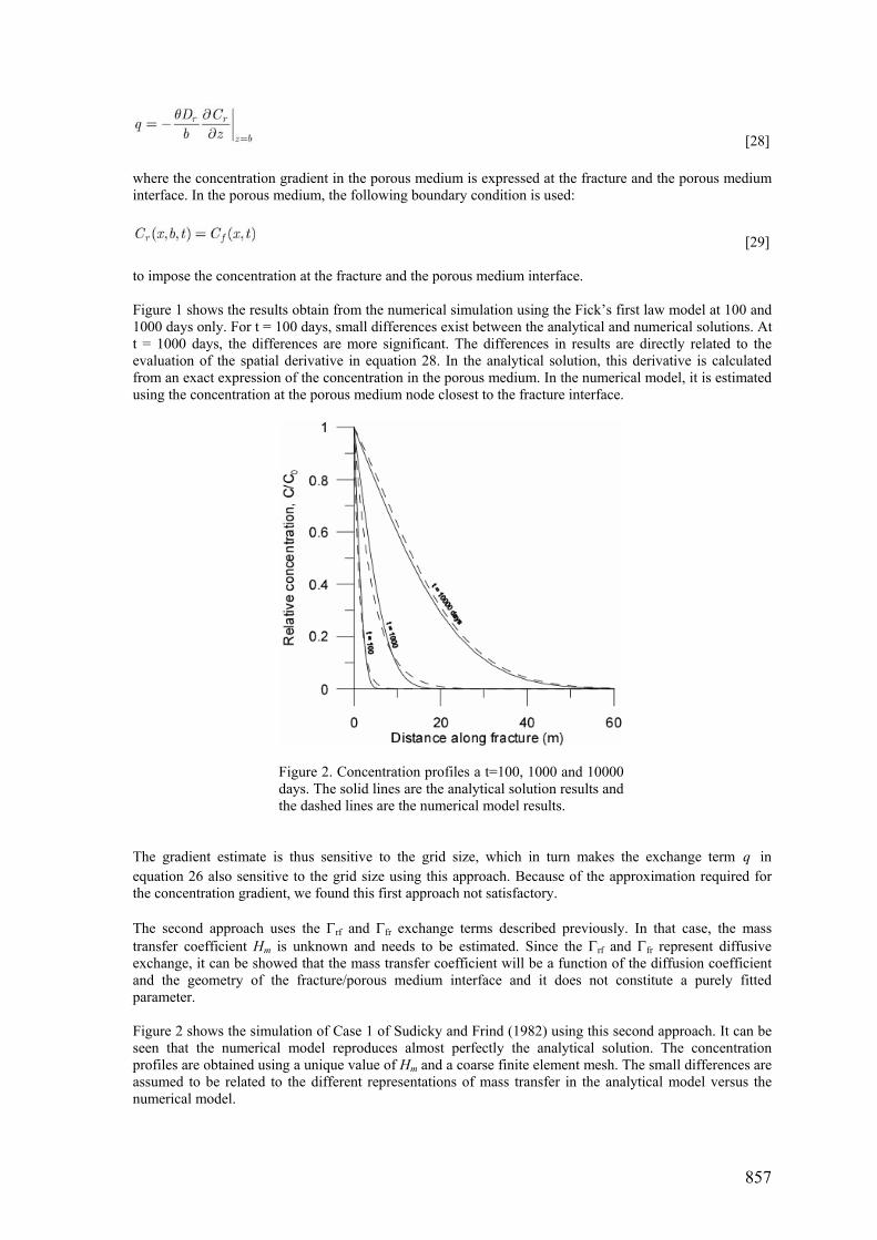
Figure 2. Concentration profiles a t=100, 1000 and 10000 days. The solid lines are the analytical solution results and the dashed lines are the numerical model results.

The gradient estimate is thus sensitive to the grid size, which in turn makes the exchange term q in equation 26 also sensitive to the grid size using this approach. Because of the approximation required for the concentration gradient, we found this first approach not satisfactory. The second approach uses the Γrf and Γfr exchange terms described previously. In that case, the mass transfer coefficient Hm is unknown and needs to be estimated. Since the Γrf and Γfr represent diffusive exchange, it can be showed that the mass transfer coefficient will be a function of the diffusion coefficient and the geometry of the fracture/porous medium interface and it does not constitute a purely fitted parameter. Figure 2 shows the simulation of Case 1 of Sudicky and Frind (1982) using this second approach. It can be seen that the numerical model reproduces almost perfectly the analytical solution. The concentration profiles are obtained using a unique value of Hm and a coarse finite element mesh. The small differences are assumed to be related to the different representations of mass transfer in the analytical model versus the numerical model.

857

5. Illustrative Example In this section, an illustrative example is presented where an initial mass of contaminant is released in a fracture network located in a porous medium. The hydraulic parameters for the porous medium and the fracture are based on those measured at the Smithville site (Ontario), where a dolostone has been contaminated by PCB (Novakowski et al., 1997).

Figure 3. Breakthrough curves as function of the mass transfer coefficient H for a point located at 8m in x- and 0.33m in z-direction. Units of H are 1/T.

The domain considered has a unit thickness and dimensions equal to 10m and 1m in the x- and z-directions, respectively. Steady-state fluid flow is assumed for the domain, with prescribed hydraulic heads equal to 1m and 0m at the left and right boundaries, respectively, and impermeable top and bottom boundaries. For transport, the initial concentration is assumed equal to zero everywhere in the porous medium. It is also zero everywhere in the fracture, except at the source located at 2.5m in the x- and 0.66m in z-direction, where an initial concentration equal to 1 is used to represent a release of contaminant. Boundary conditions for transport are a prescribed concentration equal to zero at the left inflow boundary and zero-dispersive fluxes elsewhere. The solute is assumed conservative, without retardation or degradation. We consider 3 fractures of uniform aperture equal to 500 µm with an exception of the right part of the upper horizontal fracture that has an aperture of 50µm. Two fractures are horizontal and extend over the domain in the x-direction and are located at 1/3 and 2/3 in the z-direction. The vertical fracture is located at 5m in the x-direction and extends on all z-direction and connects the 2 horizontal fractures. The longitudinal dispersivity in the fractures is equal to 0.1. The porous medium has negligible permeability. Its porosity is equal to 0.01 and the effective solute diffusion coefficient is equal to 1.38x10-4 m2/day. The simulation is run for a total time of 1000 days after the release of contamination, and the time stepping used is 10 days. Figure 3 presents solute breakthrough curves for different values of the mass transfer coefficient. As the transfer coefficient increases, diffusion from the fracture into the porous medium becomes larger. As a result, the concentration peak becomes lower and the time for peak arrival becomes larger. Also, the breakthrough curves show more tailing after the peak arrival when diffusion into the porous medium increases. As a result, it takes more time for the system to naturally flush the contaminant out. Two other simulation results are shown in Figure 4 to highlight the mesh refinement capabilities of the model. The top panel shows a fixed mesh with uniform element size along with the computed concentration

858

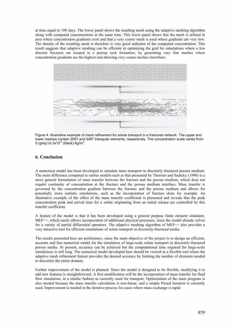
at time equal to 100 days. The lower panel shows the resulting mesh using the adaptive meshing algorithm along with computed concentrations at the same time. This lower panel shows that the mesh is refined in area where concentration gradients exist and that a very coarse mesh is used where gradients are very low. The density of the resulting mesh is therefore is very good indicator of the computed concentration. This result suggests that adaptive meshing can be efficient in optimizing the grid for simulations where a few discrete fractures are located in a porous rock formation, by generating very fine meshes where concentration gradients are the highest and allowing very coarse meshes elsewhere.

Figure 4. Illustrative example of mesh refinement for solute transport in a fractured network. The upper and lower meshes contain 2067 and 4487 triangular elements, respectively. The concentration scale varies from 0 (grey) to 3x10-4 (black) Kg/m3. 6. Conclusion A numerical model has been developed to simulate mass transport in discretely-fractured porous medium. The main difference compared to earlier models such as that presented by Therrien and Sudicky (1996) is a more general formulation of mass transfer between the fracture and the porous medium, which does not require continuity of concentration at the fracture and the porous medium interface. Mass transfer is governed by the concentration gradient between the fracture and the porous medium and allows for potentially more realistic simulations, such as the incorporation of fracture skins for example. An illustrative example of the effect of the mass transfer coefficient is presented and reveals that the peak concentration peak and arrival time for a solute originating from an initial release are controlled by this transfer coefficient. A feature of the model is that it has been developed using a general purpose finite element simulator, MEF++, which easily allows incorporation of additional physical processes, since the model already solves for a variety of partial differential operators. The adaptive meshing algorithm of MEF++ also provides a very attractive tool for efficient simulations of solute transport in discretely-fractured media. The results presented here are preliminary, since the main objective of the project is to design an efficient, accurate and fast numerical model for the simulation of large-scale solute transport in discretely-fractured porous media. At present, accuracy can be achieved but the computational time required for large-scale simulations is still long. The numerical model developed here should be viewed as a flexible tool where the adaptive mesh refinement feature provides the desired accuracy by limiting the number of elements needed to discretize the entire domain. Further improvement of the model is planned. Since the model is designed to be flexible, modifying it to add new features is straightforward. A first modification will be the incorporation of mass transfer for fluid flow simulation, in a similar fashion as currently used for transport. Optimization of the main program is also needed because the mass transfer calculation is non-linear, and a simple Picard iteration is currently used. Improvement is needed in the iterative process for cases where mass exchange is rapid.

859

860

7. Acknowledgements Funding for this research has been provided by the Natural Sciences and Engineering Research Council of Canada (NSERC), in the form of an operating grant and a strategic program grant to R.T, as well as by the Groupe Interdisciplinaire de Recherche en Elements Finis (GIREF). 8. Remark An up-to-date version of this paper is available at: http://www.ggl.ulaval.ca/Reggul/etudiants/guikenny.html 9. References Bear, J. 1972. Dynamics of fluids in porous media. American Elsevier, New York, NY, 764 p. Belhamadia, Y., Fortin, A. and Chamberland, É. 2004a. Anisotropic Mesh Adaptation for the Solution of the Stefan Problem. J. of Comp. Phys., 194(1), pp.233-255. Belhamadia, Y., Fortin, A. and Chamberland, E. 2004b. Three-Dimensional Anisotropic Mesh Adaptation for Phase Change Problems. J. of Comp. Phys., Submitted. Bourisli, R. 2002. A general review of the SUPG method in a consistent Petrov-Galerkin formulation applied to solutions of viscoelastic flow problems. Rensselaer Polytechnic Institute, pp 25. Charbeneau, Randall J. 2000. Groundwater hydraulics and pollutant transport. Prentice Hall, 1st edition, 593 p. Fortin, A., 2004. http://www.giref.ulaval.ca/ressources/projets/mefpp.html. Freeze, R. A. and Cherry, J. A. 1979. Groundwater. Prentice Hall, Englewoods, NJ, 604 p. GMSH, http://www.geuz.org/gmsh/, 2004. Novakowski, Kentner S., Bickerton, Gregory S. 1997. Borehole measurement of the hydraulic properties of low-permeability rock. Water Resources Research, 33 (11). pp. 2509-2517. Sudicky, E. A. and Frind, E. O. 1982. Contaminant transport in fractured porous media; analytical solutions for a system of parallel fractures. Water Resources Research, 18(6). pp.1634-1642. Therrien, R. and Sudicky, E. A. 1996. Three-dimensional analysis of variably-saturated flow and solute transport in discretely-fractured porous media. Journal of Contaminant Hydrology, 23(1-2). pp.1-44. VU, 2004. http://www3.sympatico.ca/chantal.pic/vu/eng/.