38th aerospace sciences meeting & exhibit 10-13 …fliu.eng.uci.edu/publications/c022.pdffor a...

For permission to copy or republish, contact the American Institute of Aeronautics and Astronuatics1801 Alexander Bell Drive, Suite 500, Reston, VA 20191

38th Aerospace SciencesMeeting & Exhibit

10-13 January 2000 / Reno, NV

AIAA-2000-0907Calculation of Wing flutter by a CoupledCFD-CSD method

F. Liu, J. Cai, Y. ZhuUniversity of California, IrvineIrvine, CA 92697-3975

A.S.F. Wong, and H.M. TsaiDSO National Laboratories20 Science Park Drive, Singapore 118230

Calculation of Wing Flutter by a Coupled CFD-CSD

Method

F. Liu∗, J. Cai†, Y. Zhu‡

Department of Mechanical and Aerospace EngineeringUniversity of California, Irvine, CA 92697-3975

A.S.F. Wong§, H.M. Tsai¶

DSO National Laboratories20 Science Park Drive, Singapore 118230

An integrated Computational Fluid Dynamics (CFD) and Computational Structural Dynamics (CSD)method is developed for the simulation and prediction of flutter. The CFD solver is based on an un-steady, parallel, multiblock, multigrid finite-volume algorithm for the Euler/Navier-Stokes equations. TheCSD solver is based on the time integration of modal dynamic equations extracted from full finite-elementanalysis. A general multiblock deformation grid method is used to generate dynamically moving grids forthe unsteady flow solver. The solutions of the flow field and the structural dynamics are coupled stronglyin time by a fully implicit method. The unsteady solver with the moving grid algorithm can be used tocalculate harmonic or indicial response of an aeroelastic system to be used by traditional flutter predictionmethods on the frequency domain. The coupled CFD-CSD method simulates the aeroelastic system directlyon the time domain and is not limited to linearized solutions. It is capable of predicting damped, diverging,and neutral motions, and limit cycle oscillations of an aero-elastic system. Computations are performedfor a two-dimensional wing aeroelastic model and the the three-dimensional AGARD 445.6 wing. Flutterboundary predictions by the coupled CFD-CSD method are compared with those by the indicial methodand experimental data for the AGARD 445.6 wing.

1 Introduction

Like in many other areas of aerodynamics, the panel

method, methods based on the transonic small distur-

bance (TSD) equation, and methods based on the full

potential (FP) equation successively found their ways

in the simulation and prediction of flutter of airfoils

and wings since CFD was introduced as a tool for aero-

dynamic research and design. As CFD and computer

technology progress, higher order methods based on the

Euler and the Navier-Stokes equations become more at-

tractive since they are able to model more accurately

transonic, nonlinear, and viscous effects. Computations

have also advanced from two-dimensional problems to

fully three-dimensional problems with or without cou-

pled solution of the structural equations. Ballhaus and

Goorjian[1] used a two-dimensional Euler code to cal-

culate the indicial response of an airfoil, where the flow

∗Associate Professor of Mechanical and Aerospace Engineer-ing, senior Member AIAA.†Visiting Research Specialist, Associate Professor, Northwest-

ern Polytechnical University, Xi’an, China.‡Graduate student, Member AIAA.§Member of Technical Staff.¶Senior Member of Technical Staff, Member AIAA.

Copyright c©2000 by the authors. Published by the AmericanInstitute of Aeronautics and Astronautics, Inc., with permission.

calculations were performed off-line, i.e., separately

from the solution of the structural equations. Bendik-

sen and Kousen[2] and Kousen and Bendiksen[3] used

an explicit time accurate Euler code to study nonlin-

ear effects in transonic flutter. With their Euler model

coupled with the solution of a 2 Degrees of Freedom

(DOF) airfoil structural model, they demonstrated the

possibility of Limit Cycle Oscillations (LCO) in a tran-

sonic flow. Lee-Rausch and Batina[4] and [5] developed

three-dimensional methods for the Euler and Navier-

Stokes equations, respectively, for predicting flutter

boundaries of three-dimensional wings. Both the in-

dicial method and the coupled CFD-CSD method was

used. Guruswamy[6] developed a Navier-Stokes code,

ENSAERO, for aeroelastic simulations.

It is clear that time accurate solutions with the cou-

pled Euler/Navier-Stokes equations and the structural

dynamic equations provide a powerful tool for simu-

lating aerodynamic flutter phenomena. However, the

computational time needed for such calculations still

prevents such methods from being used for routine

analysis and design purposes. In addition, the relia-

bility and accuracy of such methods have not yet been

well established.

An effective method to shorten the wall clock time for

1

such computations is to use parallel processing. Alonso

and Jameson[7] developed a two-Dimensional parallel

code for wing flutter calculations that couples the so-

lution of the Euler equations with the solution of the

structural equations. Byun and Guruswamy[8] also de-

veloped a parallel version of the ENSAERO code, which

was recently used and extended by Goodwin, et al[9].

In this paper, we present a new integrated CFD-

CSD simulation code for flutter calculations based on

a parallel, multiblock, multigrid flow solver for the

Euler/Navier-Stokes equations. Structural modal dy-

namic equations are solved simultaneously in a strongly

coupled fashion with the Navier-Stokes equations by a

fully implicit time marching method. A dual-time step-

ping algorithm is used to achieve time accuracy and

allow simultaneous integration of the flow and struc-

tural equations without any time delay. A novel moving

mesh method is developed to dynamically move/deform

the computational grid at each time step. A spline ma-

trix method is used to provide the interpolation be-

tween the CFD and CSD grids. The complete inte-

grated CFD-CSD is implemented on a parallel com-

puter by using the Message Passing Interface (MPI)

standard. The code has been shown to offer good paral-

lel speed-up on PC clusters networked with commodity

100Mb/s ethernet.

This computer program is capable of calculating con-

ventional harmonic or indicial responses of an aeroe-

lastic system as well as doing direct CFD-CSD sim-

ulations. Computations are performed on a two-

dimensional airfoil model and a well established three-

dimensional test case, the AGARD 445.6 wing[24, 25],

to validate and establish the usefulness of the code. In

the following section, we will describe each component

of the integrated system. We will then present and an-

alyze the computational results for the 2D aeroelastic

wing model and the 3D AGARD 445.6 wing.

2 The Unsteady Navier-StokesSolver

Tsai, Dong, and Lee[10] developed a multiblock, multi-

grid Euler/Navier-Stokes code called NSAERO (unfor-

tunately, this is very close to the name of Guruswamy’s

code) for steady flow calculations based on Jame-

son’s finite-volume and Runge-Kutta time-marching

method[11, 12]. The multiblock algorithm uses two lay-

ers of halo cells to exchange flow information across a

common interface between two blocks. Multigrid is im-

plemented in a ‘horizontal mode’ as termed by Yadlin

and Caughey[13], in which the block loop is nested in-

side the loop for the multigrid cycle so that information

is exchanged among blocks and the flow field is updated

on all blocks within each time step at each multigrid

level. Information is not exchanged among blocks for

the internal multi-stages of the explicit Runge-Kutta

time-stepping within each time step. This code has

been validated and extensively used for steady flow cal-

culations of wing, wing-body combination, S-ducts, and

complete aircraft[10].

In this research, the code is extended to per-

form time-accurate calculations. Time-accuracy is

achieved by using the dual-time method proposed by

Jameson[14]. The basic implementation of the dual-

time step method is the same as in Liu and Ji[15].

After being discretized in space by a finite volume

method, the time dependent Navier-Stokes equations

can be written in the following semi-discrete form

dw

dt+R(w) = 0 (1)

where w is the vector of flow variables at each mesh

point, and R is the vector of the residuals, consisting

of the spatially discretized flux balance of the Navier-

Stokes equations. A second order accurate fully implicit

scheme is then used to integrate the above equation in

time,

3wn+1 − 4wn + wn−1

2∆t+R(wn+1) = 0 (2)

This implicit scheme is A-stable. We can reformulate

(2) into the following

dw

dt∗+R∗(w) = 0 (3)

where

R∗(w) =3

2∆tw +R(w)− 2

∆twn +

1

2∆twn−1 (4)

t∗ is a pseudo-time. The solution of the implicit equa-

tion (2) is now made equivalent to the steady state so-

lution of (3) with the pseudo-time t∗. We can then ap-

ply all the acceleration techniques including the multi-

grid method that are already implemented in the steady

NSAERO to solving Equation (3). Once the solution

to Equation (3) converges in pseudo-time, we achieve

the time accurate solution to Equation (2) for one time

step. As was demonstrated in [15], CFL numbers of

more than 4000 could be used for solving the unsteady

equations with this technique. Each time step needed

about 20-40 multigrid pseudo-time cycles to reach a

converged solution for the Euler equations. In the cal-

culations performed in this paper, 60 pseudo-time cy-

cles are used for each real time step when coupled with

the structural modal equations to ensure adequate con-

vergence in pseudo-time.

Time accurate calculations for three-dimensional

problems are still very time consuming with even the

2

best algorithms available at the current time. In order

to keep the computational time within realistic limits

for large unsteady calculations, the code is also par-

allelized by using domain decomposition and MPI to

take advantage of parallel computers or networked clus-

ters of workstations. The flow field is partitioned into

multiple blocks which are distributed over a number

of processors available on a parallel computer or net-

worked workstations. The existing multiblock structure

in the steady NSAERO code[10] provides the basis for

the parallel implementation. The dual time implicit-

explicit solver is performed on each processor for the

individual blocks assigned to that processor. Again,

two layers of halo cells are used beyond the bound-

aries of each block to facilitate the implementation of

boundary conditions and the communication between

processors. Connectivity information of the blocks and

processors are stored in preprocessed pointer arrays and

MPI is used to perform the communication between

blocks that are on different processors.

The unsteady implementation has been validated by

calculating the same airfoil test case as in [15], i.e.,

the flow over a pitching NACA64A010 airfoil. Since

the new unsteady parallel NSAERO code is fully three-

dimensional, we also tested the airfoil case by laying the

pitching airfoil in the three different coordinate planes.

Comparison of the computed results showed no differ-

ence between the calculations with different coordinate

orientations, and the results agree with the experimen-

tal data found in [16]. More detailed description of the

parallel implementation and code validation studies will

be presented in a separate paper.

In this paper, we will concentrate on flutter predic-

tions to be discussed in the following sections. We will

note, however, that the parallel code runs efficiently on

clustered PCs. Figure 1 shows the parallel speedup for

the airfoil case of the new parallel unsteady NSAERO

running on the AENEAS computer consisting of 32

300MHZ Pentium II processors connected by a 100Mb

switched ethernet network. It can be seen that the

parallel efficiency remains high for the available pro-

cessors for this case with 71001 total grid points. With

32 processors, we achieve a speedup factor of 25. The

parallel efficiency is higher for most three-dimensional

runs with more grid points.

3 A Multi-block Moving MeshAlgorithm

A novel moving grid algorithm, AIM3D, which

remeshes the moving configuration adaptively in each

block of grids, is also implemented in a parallel fashion

and combined with the flow solver to handle flow prob-

lems with arbitrary motion of domain boundaries. The

moving grid algorithm within each block is based on

the method of arc-length based transfinite interpolation

which is performed independently on local processors

where the blocks reside. A spring network approach is

used to determine the motion of the corner points of

the blocks which may be connected in an unstructured

fashion in a general multi-block method. A smooth-

ing operator is applied to the points of the block face

boundaries and edges in order to maintain grid smooth-

ness and grid angles. The details of this moving grid

method is described in [17]

4 The CSD Model and Its Solu-tion

Modal equations are used to calculate the structural

deformation under an aerodynamic forcing. For each

mode i, the modal dynamic equation is written in the

following form

qi + 2ζiωiqi + ω2i qi = Qi (5)

where qi is the generalized normal mode displacement,

ζi is the modal damping, ωi is the modal frequency, and

Qi is the generalized aerodynamic force. The structural

displacement vector can be written as a summation of

N modal shapes extracted from a full finite element

analysis of the structure.

{us} =

N∑

i=1

qi{hi} (6)

where {hi} are the modal shapes.

Equation (5) is converted into a first order system

of equations for each i and integrated in time by a

second-order fully implicit scheme. Following Alonso

and Jameson[7], we assume

x1i = qi

x1i = x2i (7)

x2i = Qi − 2ζiωix2i − ω2i x1i

for each of the modal equations. We can rewrite the

above equations in matrix form as

{Xi} = [Ai]Xi + {Fi}, i = 1, N (8)

where {Xi} =

{x1i

x2i

}, [A] =

[0 1−ω2

i −2ωiζi

]and

{Fi} =

{0Qi

}. After proper diagonalization, the

above equation can be decoupled.

dz1i

dt= ωi(−ζi +

√ζ2i − 1)z1i +

(−ζi +√ζ2i − 1)

2√ζ2i − 1

Qi (9)

3

dz2i

dt= ωi(−ζi −

√ζ2i − 1)z2i +

(ζi +√ζ2i − 1)

2√ζ2i − 1

Qi (10)

We use the same second order accurate fully implicitscheme as Equation (2) to integrate the above equationsin time.

3zn+11i − 4zn1i + zn−1

1i

2∆t= −R1i(z

n+11i , zn+1

2i , Qn+1i ) =

ωi(−ζi +√ζ2i − 1)zn+1

1i +(−ζi +

√ζ2i − 1)

2√ζ2i − 1

Qn+1i (11)

3zn+12i − 4zn2i + zn−1

2i

2∆t= −R2i(z

n+11i , zn+1

2i , Qn+1i ) =

ωi(−ζi −√ζ2i − 1)zn+1

2i +(ζi +

√ζ2i − 1)

2√ζ2i − 1

Qn+1i (12)

The variables z1i, z2i, and Qi in the above equations

are coupled through the flow equations. The deforma-

tion of the wing, i.e., z1i, z2i influences the flow field

and, thus, the aerodynamic force Qi. Conversely, the

aerodynamic force Qi determines the deformation of

the wing. Therefore, the above equations for the time

marching of the structural equations must be solved si-

multaneously with Equation (2) for the Navier-Stokes

equations.

It is very convenient to reformulate Equations (11)

and (12) into an identical pseudo-time format as Equa-

tions (3) and (4), i.e.,

dz1i

dt∗+R∗1i(z1i, Qi) = 0 (13)

dz2i

dt∗+R∗2i(z2i, Qi) = 0 (14)

where

R∗1i(z1i, Qi) =3

2∆tz1i +R1i(z1i, z2i, Qi)

− 2

∆tzn1i +

1

2∆tzn−1

1i (15)

R∗2i(z1i, Qi) =3

2∆tz2i +R2i(z1i, z2i, Qi)

− 2

∆tzn2i +

1

2∆tzn−1

2i (16)

Equations (3), (13) and (14) can be regarded as one sin-

gle system of time dependent equations in the pseudo-

time t∗ which can be solved by existing efficient ex-

plicit time marching methods until a steady state is

reached. Once the computation reaches a steady state

in the pseudo-time t∗, the solutions to Equations (3),

(13) and (14) then become the time accurate solution

of the implicit fully coupled CFD-CSD Equations (2),

(11) and (12) in one physical time step without any

time lag between the CFD and CSD equations.

In the current implementation, the same 5 stage

Runge-Kutta time stepping scheme for the Navier-

Stokes equations is used for the CSD equations. It is

found, however, that the CSD pseudo-time equations

converge faster than their counterparts in the flow equa-

tions. Therefore, it is more efficient and, in fact, more

robust to march the flow equations with more pseudo-

time steps than for the CSD equations. It should be

noticed that this will not affect the final time accuracy

in the physical time as long as a steady state is reached

in the pseudo-time.

5 Interfacing between the CSDand CFD Grids

The proceeding sections lay out the mathematical for-

mulation of the coupling of the CFD and CSD equa-

tions. However, there remains a missing link in actual

computation, that is, the relation between the CFD

computational grid and the CSD computational grid.

Although Bendiksen and Hwang[21] developed a finite

element algorithm for both the flow equations and the

structural equations so that the same surface grid can

be used, most CFD codes use different algorithms and

different computational grids for the flow and the struc-

tures. Consequently, interpolation of computational

grids and aerodynamic loads must be performed be-

tween the two systems. A suitable method that han-

dles this need in a general fashion is still in the mak-

ing. The current engineering practice, as exemplified in

MSC/NASTRAN and used in the current paper, uses a

combination of methods. The infinite plate spline (IPS)

by Harder and Desmarais[18] and thin plate spline

(TPS) by Duchon[19] is more suitable for wing-like

components where the structure is usually modeled by

plate and shell elements. The beam spline method by

Done[20] is used for body-like component as the struc-

ture is modeled by beam elements. The structural grid

of a complex structure that uses a combination of differ-

ent elements can be related to the aerodynamic grid by

using different spline methods. Details of the approach

are to be found in MSC/NASTRAN Aeroelastic Anal-

ysis, User’s Guide. Once a spline method is applied,

the displacement vector defined on the structural grid

{us} can be related to the displacement vector on the

aerodynamic grid {ua} via a spline matrix [G],

{ua} = [G]{us} (17)

Once the structure equations are solved, the displace-

ments on the structural grid {us} is transformed to

the displacement on the aerodynamic grid {ua} by the

above equation, from which the deforming grid code

AIM3D discussed in Section 3 can then be used to

regenerate the volume grid in the flow field for CFD

computations. Once the flow equations are solved, the

4

aerodynamic loading on the CFD grid {Fa} can then be

transformed to the aerodynamic loading on the struc-

tural grid {Fs} via the following equation based on the

principle of virtual work.

{Fs} = [G]T {ua} (18)

where [G]T is the transpose of [G]. Equation (18) guar-

antees the conservation of energy between the flow and

the structural systems due to the fact that it is derived

by the principle of virtual work.

The size of the vector {ua} is 3 times m, m being the

number of aerodynamic grid points on the wing surface.

The size of the structural displacement vector {us} is

3 times n, n being the number of finite element grid

point on the wing surface. The size of the [G] matrix is

then (3m)× (3n). The [G] matrix is pre-generated and

stored in the code.

6 The Integrated Aero-structureSystem

Figure 2 shows the integration strategy for our aero-

elastic simulation system. At the start of the pro-

gram, specification of the structures are input to NAS-

TRAN which extracts the modal shapes and parame-

ters needed by the CSD solver in the coupled simulation

code. Inputs are also given to the flow solver NSAERO

and its preprocessor PREPNS. The flow solver will

first compute the static loading on the structure. The

aerodynamic forcing {Fa} is then transformed to the

form suitable for the CSD modal equations using the

SPLINE matrix G. The CSD solver then computes

the structural displacement {us}, which is subsequently

transformed to the grid points for the flow solver. With

the new displacement {ua}, the dynamic moving mesh

program REMESH (AIM3D) is called to regenerate the

mesh for the flow solver. The flow solver and the CSD

solver are coupled within each time step through the

above process as shown by the arrows in Figure 2. Since

both the flow equations and the structural equations

are solved by a pseudo-time iteration algorithm, the

above coupling between the CFD and CSD solver are

easily absorbed in the pseudo-time iteration process un-

til a fully converged solution is achieved at the new time

level as discussed in Section 4.

Figure 2 also shows a “decoupled” approach for flut-

ter prediction marked by the dashed lines. In such an

approach, prescribed structural motion is provided to

the flow solver without being coupled with the CSD

model. The generalize aerodynamic force Qij on the

frequency domain is extracted from the CFD calcula-

tions by using either the harmonic method or the in-

dicial response method. Qij will then be fed into the

conventional V-g method to obtain flutter boundaries

of the aero-elastic system. This method provides a fast

tool for flutter predictions, but it is restricted to linear

systems. The fully coupled method provides a compli-

ment to the linearized approach.

7 Computational Results

7.1 A two-Dimensional Wing Model

As a first test case, we apply the coupled CFD-CSD

method to the two-dimensional Isogai wing model[22,

23], Case A. This model simulates the bending and tor-

sional motion of a wing cross-section in the outboard

portion of a swept wing. It consists of two degrees of

freedom, plunging and pitching, for a NACA 64A010

airfoil. We compute this case with the Euler equations

and compare the results by Alonso and Jameson[7].

The details of the structural model can be found in

[7] as well as in [22] and [23].

Figures 3-6 show the flutter computational results

for the Isogai wing model at a flight Mach number of

0.825. Plotted in the figures are the time history of

the pitching and plunging amplitude computed by the

integrated CFD-CSD code with the fully coupled CFD

and CSD approach. Figure 3 is a case with a low speed

index Vf = 0.530. Vf is defined as

Vf =U∞bω√µ

where U∞ is the freestream velocity, b is the half chord,

ω is the structural frequency, µ is the mass ratio. For

this low Vf , figure 3 shows that both the pitching and

plunging amplitude decays with time, indicating that

the aeroelastic system is stable for this particular con-

dition. At a higher Vf , the system may become less

and less stable until one or both of the pitching and

plunging motions diverge as shown in Figure 4 when

Vf = 0.725. In between these two Vf conditions, there

is a particular point where the system is neutrally sta-

ble. This is shown in Figure 5 when Vf = 0.630.

A converging point and a diverging point like the

above are first identified, from which we can interpo-

late the Vf in between to obtain an estimate of the

neutral point. We then perform a computation with

the new Vf to see if it is above or below the stability

limit, or perhaps right at the neutral point. It may take

several runs for a given freestream Mach number before

the Vf corresponding to the neutral stability point can

be accurately located by this ’bi-section’ method. How-

ever, most of the runs do not need computations with

many time periods since we can easily identify whether

the system is oscillating with a diverging or converg-

ing amplitude by looking at only the first few periods.

5

With this method computations for a number of free-

stream Mach numbers for the Isogai wing model are

performed. The flutter boundary predicted by our code

is plotted and compared with that obtained by Alonso

and Jameson[7] in Figure 7. Clearly, the results by the

two codes agree very closely for this case.

Figure 6 shows a situation where the system initially

diverges but then reaches a steady oscillatory mode

with finite amplitude, the so-called Limit Cycle Oscil-

lation (LCO). The LCO for this case was first discov-

ered by Kousen and Bendiksen and was also shown by

Alonso and Jameson[7]. This test case demonstrates

the capability of the integrated CFD-CSD program to

predict LCO although the computation may have to be

performed for a long time before LCO can be identified

in the time integration.

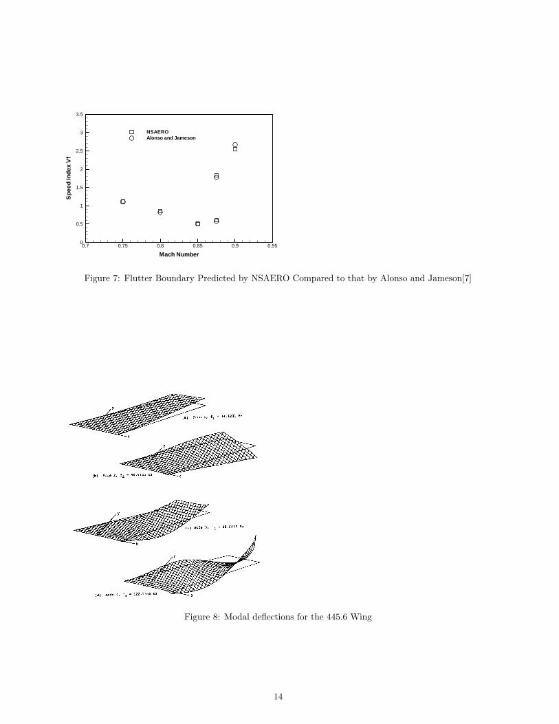
7.2 The AGARD 445.6 Wing

Although the results in the above section are calcu-

lated by using the full three-dimensional code with 8

cells in the spanwise direction, the flow is only two-

dimensional. In this section, the integrated aeroelas-

tic system is used to predict the flutter boundary for

the AGARD 445.6 wing[25, 24] by both the indicial

method and the coupled CFD-CSD method. This wing

is a semispan model made of the NACA 65A004 airfoil

that has a quarter-chord sweep angle of 45 degrees, a

panel aspect ratio of 1.65, and a taper ratio of 0.66.

We consider the weakened wing model as listed in Ref-

erence [24]. It was tested in the Transonic Dynam-

ics Tunnel (TDT) at NASA Langley Research Cen-

ter. This is a well-defined test case proposed as an

AGARD standard aeroelastic configuration for flutter

calculations[25]. The wing is modeled structurally by

the first four natural vibrational modes shown in Fig-

ure 8 as taken from Reference [25]. Those are identified

as the first bending, first torsion, second bending, and

second torsion modes, respectively, by a finite-element

analysis. The natural frequencies of these modes are

also shown in Figure 8. A grid of 176601 is used for

this case. Although the code is capable to run in the

Navier-Stokes mode with a two-equation k-ω model,

only Euler solutions are presented in this work.

In a harmonic method to calculate the generalize

aerodynamic force Qij for the i-th vibrational mode,

the wing is assumed to undergo a sinusoidal motion of

the i-th mode at a given reduced frequency κ. The un-

steady flow induced by this sinusoidal motion is then

calculated, from which the generalized aerodynamic

force on each of the j-th mode (j = 1, 4) can be de-

duced. To illustrate the shape and motion of the wing,

Figure 9 shows the computed pressure distribution in

the symmetry plane and on the wing surface at one

time instant for the four different wing structural de-

formation modes vibrating sinusoidally at their corre-

sponding natural frequencies, respectively.

In order to use a classical V -g method to determine

the flutter boundary, Qij must be calculated over a

range of frequencies of interest. Consequently, compu-

tation of the flow field must be performed for a number

of reduced frequencies and for each vibrational mode

of importance in a harmonic method. This demands

a large amount of computational time. An alterna-

tive is to use the Indicial Method originally proposed

by Tobak[26], and also by Ballhaus and Goorjian[1],

in which, a step function input excitation is fed into

the aerodynamic system for each structural mode. The

response of the aerodynamics system is called the Indi-

cial Response. A Fourier analysis on this Indicial Re-

sponse is enough to deduce the system response Q(κ)

for the complete range of the reduced frequency κ. In

this way, only one time-integration of the Euler/Navier-

Stokes equations is needed for each mode of the struc-

tural system in order to obtain the complete GAF ma-

trix Qij(κ). Seidel, Bennett and Ricketts[27] intro-

duced a impulse function method to avoid the disconti-

nous nature of the step function used by Ballhaus and

Goorjian[1]. The impulse method is used in this work.

Figures 10 and 11 show the comparison of the gen-

eralized aerodynamic forces Q11 and Q21 calculated by

the harmonic method and the impulse method for the

445.6 wing at a freestream Mach number M∞ = 0.901.

It can be seen that except near the high reduced fre-

quency end, the indicial method based on the impulse

input agree well with the harmonic method. The indi-

cial method, however, significantly reduces the compu-

tational time.

Figures 12, 13, 14, and 15 show the computed gen-

eralized aerodynamic forces Q11, Q12, Q21, and Q22,

respectively, by the indicial method for the first two

vibrational modes. The first 4 modes are calculated al-

though only 2 of them are shown here. Those Qij ’s are

then used in a classical V -g method code to determine

the flutter boundary of the wing.

Unlike in an indicial or harmonic method where a

prescribed motion of the wing is used, the motion of

the wing is not pre-determined in a direct CFD-CSD

coupled simulation. It is computed based entirely on

the flow and structural dynamic equations and their

interaction. The wing is started with either an ini-

tial displacement and zero initial vibrational velocity

or zero displacement but non-zero vibrational velocity

in each of the 4 modes. A steady state solution is first

obtained for a given initial position of the wing and

then the wing is let go. The wing will then start os-

cilating in time resulting in either damped, diverging,

6

or neutral vibrations.

Figures 16 to 19 show the time histories of the gen-

eralize coordinates qi of the first 4 modes in the cou-

pled CFD-CSD unsteady computations for some differ-

ent flight Mach numbers and different speed index Vf .

Although the time history may be different when dif-

ferent initial conditions are used, it was found that the

general behavior of the wing is the same in so far as

stability is concerned. If a mode is unstable (diverging

in time) for the zero velocity but non-zero displace-

ment initial condition, it will also be unstable for the

zero displacement but non-zero velocity initial condi-

tion. In principle, it is not impossible that stability

depends on initial conditions for a nonlinear system.

However, no special effort is made to identify this in

the current work.

Consider the supersonic flight condition M∞ = 1.141

tested in the experiment[24]. Figure 16 shows the time

history of the 4 generalized coordinates for the 445.6

wing for a velocity index Vf = 0.58. For this case,

the flow is started with zero initial displacement but a

non-zero initial velocity in all of the four modes of the

wing. Clearly, Figure 16 shows that this is a damped

case. The amplitudes of all modes decrease in time.

Therefore, the system is stable for this condition. At

a little higher speed index Vf = 0.652, the system ex-

hibit high vibrational amplitude and slower damping as

shown in Figure 17. However, it is still a damped case

although it is getting close to the neutral condition. At

an even higher speed index Vf = 0.70 as shown in Fig-

ure 18, we can see that the amplitude of the first three

modes grow very fast, indicating that we have passed

the neutral stability point. At this point, the flutter

boundary for this flight Mach number can be roughly

estimated to be in between Vf = 0.652 and Vf = 0.700.

This process can be iterated to obtain better estimates

of the flutter boundary. But for this case, a mean value

from Vf = 0.652 and Vf = 0.700 will suffice considering

the large difference between the experimental data and

the computed data to be discussed later.

The flutter mode can be determined by looking at

these figures and identify which mode first starts to be

unstable as we increase the Vf . Once this mode is iden-

tified, a Fourier analysis of this mode can be performed

in its last few periods of vibration near the neutral point

to identify its frequency. A quick estimate can be ob-

tained by simply measuring the time between the two

zero points in the end of the vibration. This may get

somewhat ambiguous in some cases in determining the

flutter mode and flutter frequency. It is noticed, how-

ever, from Figures 16-18 that the vibrational frequen-

cies of the 4 modes initially are rather different and

closer to their natural frequencies for the low Vf case.

As the speed index increases, the low frequency modes

shift to higher frequencies, while the high modes tend

to shift towards the low frequency end. Near the neu-

tral point, the first two modes tend to oscillate at the

same frequency.

Figure 19 shows the calculation for the condition

M∞ = 1.072 and Vf = 0.46. Clearly, this shows that

the Vf is at or very close to the flutter boundary and

that the first or the second mode is the flutter mode,

which are almost neutral and oscillate at almost equal

frequency while the higher modes damp out in time.

Figure 20 shows a similar calculation for the subsonic

condition M∞ = 0.901 and Vf = 0.34. Again, this

shows that the chosen Vf is at or very close to the

flutter boundary and that the first mode is the flutter

mode since all other modes are being damped. It is

noticed that the frequency of the higher modes remain

high in this case.

Using the above approach, we determined the flut-

ter boundary and frequency of the weakened wing over

the flight Mach number range M∞ = 0.338 to 1.141

studied experimentally in [24]. The results are shown

in Figures 21 and 22 together with the experimental

data and those calculated by the V -g methods based

on the calculated indicial responses. It can be seen

that the results computed by the coupled CFD-CSD

method agree very well with the experimental data in

the subsonic and transonic range.

In the supersonic range, however, both the coupled

method and the indicial method yield much higher flut-

ter velocities than those determined in the experiment.

It is also to be noticed that Reference [4] also over-

predicted the Vf for supersonic flight conditions by al-

most equal amount compared to our result. Although

[5] and [9] showed some improvement by performing full

Navier-Stokes calculations, the amount of improvement

was small compared to the still large differences be-

tween their computational results and the experiment.

It is not clear why this is the case. However, subtle

differences between the subsonic and supersonic cases

can be observed from the time histories shown in Fig-

ures 16 to 20. In the subsonic case shown in Figure 20,

the damped modes show monotonically decreasing am-

plitudes similar to those found for the two-dimensional

airfoil case shown in Figure 3. For the supersonic cases,

however, the first mode shows a clear growth before it

starts to decay (Figures 16 and 17) or being neutral

(Figure 19). This behavior is found to be independent

of the initial conditions used in the calculations. It

might be conjectured that this nonlinear behavior can

be responsible for the early detection of flutter in the

model wing tested in [24]. Further investigation is nec-

essary in this regard.

7

It has been suggested that LCO may be indicated in

the V -g analysis if it exists. The coupled CFD-CSD

approach may then be used to confirm the existence

of LCO. However, no LCO phenomenon for the 445.6

wing has been found in this research or by any other

researchers.

8 Concluding Remarks

A parallel integrated CFD-CSD simulation program

has been developed for the simulation and prediction of

flutter of an aeroelastic system. This program consists

of a three-dimensional, parallel, multi-block, multigrid,

unsteady Navier-Stokes solver, a parallel dynamic grid

deformation code, a CSD solver strongly coupled with

the flow solver using dual time stepping, and a spline

matrix method for interfacing the CFD and CSD grid

and aerodynamic loading variables. This program has

two options. Option 1 allows it to obtain the harmonic

or indicial responses of an aeroelastic system by pre-

scribing the motion of the structure. Option 2 uses the

coupled CFD-CSD method to directly simulate the un-

steady behavior of an aeroelastic system. Flutter speed,

mode, and frequency can be determined by analyzing

the time history of the structural vibration.

The code has been used to simulate transonic flut-

ter of a 2D airfoil, and the three-dimensional AGARD

445.6 wing by both the indical method option using an

impulse input and the coupled CFD-CSD option. Some

useful observations are summarized below:

• In the indical method approach, as many runs

as there are structural modes must be performed

to determine the generalized aerodynamic forces

needed by the V -g method to determine flutter

boundary. Typically for a wing, 4 modes are

needed. Each run must be performed with ade-

quate time resolution in order to accurately calcu-

late the aerodynamic response for high frequencies.

In addition, long time periods are also needed for

the disturbances due to the initial impulse to suf-

ficiently decay.

• The coupled CFD-CSD option consists of a series

of full simulations of an aeroelastic system with

some arbitrarily chosen initial perturbation of the

aero-structure system, much like in wind tunnel

test. Flutter is detected by examining the com-

puted structural displacements to see if the initial

perturbations will decay, grow, or maintain a neu-

tral stance. This is readily noted within 2 to 3

periods of oscillations for most situations, which

may actually be less time than one run in the indi-

cial method mode. To determine the neutral point,

3 or more runs are usually needed.

• The stability quality determined by the above ap-

proach does not depend on the choice of initial

conditions for the computations done in this pa-

per.

• Signal analysis of the calculated modal displace-

ments in the direct coupled method must be per-

formed in order to determine the flutter mode,

speed, and frequency. Ambiguity may exist in this

method in determining which mode is the flutter

mode and at what frequency. For the AGARD

445.6 wing case, however, it was found that flutter

appears to happen with mostly the first and sec-

ond modes. The frequencies of these two modes

tend to approach each other as the velocity index

approaches the neutral point.

• Both methods give almost identical results of the

flutter speed and flutter frequency for the AGARD

445.6 wing. If one has a rough idea of where flut-

ter might occur, the coupled CFD-CSD method

can give us an estimate of the flutter point more

quickly than the indicial method.

• Flutter speed and flutter frequency predictions by

the coupled approach agree very well with exper-

imental data for subsonic and transonic speeds.

The transonic dip phenomena is well captured.

• For subsonic cases, the coupled approach predicts

either monotonically decaying modes or monoton-

ically growing modes for velocity index values be-

low or above the numerically determined neutral

point.

• Both the indicial method and the coupled method

over-predict the flutter speed and flutter frequency

for the AGARD 445.6 wing at supersonic speeds.

The coupled approach, however, predicts consis-

tent initial growths of the structural motions be-

fore they decay for velocity index values above the

experimental data but below the numerically de-

termined neutral points. Monotonic growth is ob-

served when the velocity index is above the numer-

ically determined neutral point. Whether this of-

fers an explanation for the discrepancy between the

experimental data and the numerical computation

for the supersonic case needs further investigation.

• The coupled CFD-CSD option may be used to sim-

ulate and predict LCO. However, long time of com-

putation may be needed in order to see if a system

will enter into an LCO mode. Other quick meth-

ods may be used to indicate the possibility of LCO.

8

The coupled approach may then be used to confirm

and simulate the LCO motion.

• The program developed scales well on networked

PC clusters with commodity 100Mb/s ethernet

connections. Parallel efficiencies of 25 is reached

on 32 networked Pentium II 300Mhz PCs for small

two-dimensional problems. Higher parallel efficien-

cies can be achieved for larger grid sizes. Work is

in progress to test it on larger parallel systems in

addition to networked PCs.

• With 32 networked Pentium II 300 MHz PCs, one

run of 3 periods in the coupled mode takes about

12 hours for the AGARD 445.6 wing with 176,601

grid points and 64 time steps per period. With the

fast advance in computer hardware, further im-

provement in the computational algorithms, and

better optimization of the computer program, the

CFD-CSD coupled approach may be not so far off

from being used for routine applications.

9 Acknowledgement

Computations of this work has been performed on the

AENEAS parallel computer system in UC Irvine.

References

[1] Ballhaus, W.F. and Goorjian, P.M.,

“Computation of Unsteady Transonic Flows by

the Indical Method,” AIAA Journal, Vol. 16, No.

2, Feb. 1978, pp.117-124.

[2] Bendiksen, O. O., and Kousen, K. A., “Transonic

Flutter Analysis Using the Euler Equation,”,

AIAA Paper 87-0911, April, 1987.

[3] Kousen, K. A., and Bendiksen, O. O., “Limit

Cycle Phenomena in Computational Transonic

Aeroelasticity,” Journal of Aircraft, Vol. 31, No.

6, pp. 1257-1263, November-December, 1994.

[4] Lee-Rausch, E. M., Batina, J. T., “Wing Flutter

Boundary Prediction Using Unsteady Euler

Aerodynamic Method”, Journal of Aircraft, Vol.

32, No. 2, pp. 416-422, March-April, 1995.

[5] Lee-Rausch, E. M., Batina, J. T., “Wing Flutter

Computations Using an Aerodynamic Model

Based on the Navier-Stokes Equations”, Journal

of Aircraft, Vol. 33, No. 6, pp. 1139-1147,

November-December, 1996.

[6] Guruswamy, G. P., “Navier-Stokes Computations

on Swept-Tapered Wings, Including Flexibility,”

AIAA Paper 90-1152, April, 1990.

[7] Alonso J. J., and Jameson, A. , “Fully-Implicit

Time-Marching Aeroelastic Solutions”, AIAA

Paper 94-0056, Jan., 1994.

[8] Byun, C., Guruswamy, G. P., “Aeroelastic

Computations on Wing-Body-Control

Configurations on Parallel Computers,” AIAA

Paper 96-1389, April, 1996.

[9] Goodwin, S.A., Weed, R. A., Sankar, L. N., and

Raj, P., “Toward Cost-Effective Aeroelastic

Analysis on Advanced Parallel Computing

Systems,” Journal of Aircraft, Vol. 36, No. 4, pp.

710-715, July-August, 1999

[10] Tsai, H. M., Dong, B., and Lee, K. M., “The

Development and Validation of a

Three-dimensional Multiblock, Multigrid Flow

Solver for External and Internal Flows,” AIAA

Paper 96-0171, January, 1996.

[11] Jameson, A., Schmidt, W., and Turkel, E.,

“Numerical Solutions of the Euler Equations by

Finite Volume Methods Using Runge-Kutta

Time-Stepping Schemes,” AIAA Paper 81-1259,

June 1985.

[12] Jameson, A., “Multigrid Algorithms for

Compressible Flow Calculations,” MAE Report

1743, Princeton Univ., NJ, text of lecture given

at 2nd European Conference on Multigrid

Methods, Cologne, FRG, Oct. 1985.

[13] Yadlin, Y., and Caughey, D.A., “Block Multigrid

Implicit Solution of the Euler Equations of

Compressible Fluid Flow,” AIAA-90-0106,

January 1990

[14] Jameson, A., “Time Dependent Calculations

Using Multigrid, with Applications to Unsteady

Flows past Airfoils and Wings,” AIAA Paper

91-1596, 10th AIAA Computational Fluid

Dynamics Conference”, June, 1991.

[15] Liu, F. and Ji, S., “Unsteady Flow Calculations

with a Multigrid Navier-Stokes Method,” AIAA

Journal, Vol. 34, No. 10, 1996, pp. 2047-2053.

[16] Davis, S. S., “NACA64A010 Oscillatory

Pitching,” in Compendium of Unsteady

Aerodynamics Measurements, AGARD-R-702,

1982.

9

[17] Wong, A. Tsai H., Cai, J., Y. Zhu, and F. Liu,

“Unsteady Flow Calculations with a Multi-Block

Moving Mesh Algorithm”, AIAA Paper

2000-1002, Jan., 2000.

[18] Harder, R. L., Desmarais, R. N., “Interpolation

Using Surface Splines”, Journal of Aircraft, Vol.

9, No. 2, February 1972, pp. 189-191.

[19] Duchon, J. P., “Splines Minimizing

Rotation-Invariant Semi-Norms in Sobolev

Spaces, in Schempp, W. and Zeller, K, editors,

Constructive Theory of Functions of Several

Variables, Oberwolfach 1976, pp. 85-100,

Springer-Verlag, Berlin, 1977.

[20] Done, G. T. s., “Interpolation of Mode Shapes: A

Matrix Scheme Using Two-Way Spline Curves”,

Aeronautical Quarterly, Vol. 16, November 1965,

pp.333-349.

[21] Bendiksen, O. O., and Hwang, G., “Nonlinear

Flutter Calculations for Transonic Wings,” Proc.

Int. Forum on Aeroelasticity and Structure

Dynamics, June 17-20, 1997, pp105-114, Rome,

Italy.

[22] Isogai, K., “On the Transonic-Dip Mechanism of

flutter of a Sweptback Wing,” AIAA Journal,

Vol. 17, No. 7, pp.793-795, 1979.

[23] Isogai, K., “On the Transonic-Dip Mechanism of

flutter of a Sweptback Wing: Part II,” AIAA

Journal, Vol. 19, No. 7, pp.1240-1242, 1981.

[24] Yates, E.C, Jr., Land, N.S. and Foughner J.T. Jr,

“Measured and Calculated Subsonic and

Transonic Flutter Characteristics of a 45◦

Swepteback Wing Planform in Air and in

Freon-12 in the Langley Transonic Dynamics

Tunnel”, NASA TN D-1616, March, 1963.

[25] AGARD Standard Aeroelastic Configurations for

Dynamic Response I – Wing 445.6, NASA TM

100492, Aug., 1987.

[26] Tobak, M., “On the Use of Indicial Function

Concept in the Analysis of Unsteady Motions of

Wings and Wing-Tail Combinations,” NACA

Report, 1188, 1954.

[27] Seidel, D.A., and Bennet, R.M., “An Exploratory

Study of Finite-Difference Grids for Transonic

Unsteady Aerodynamics,” AIAA 83-0503, Jan.

1983.

10

1 2 4 8 16 32Number of Processors

1

2

4

8

16

32

Spe

edup

Ideal SpeedupUCI AENEAS

Figure 1: Parallel Speedup for the Parallel Unsteady NSAERO Code on a 32 node PC Cluster with 100MbSwitched Ethernet, 71001 grid points

InputsGrid points of CFD & CSD models

CSD Inputs

NASTRANSPLINEMatrix [G]

Force

[Fs] = [G]T[Fa]

CFD SolverNSAERO

CSD Solver

Displacement[ua] = [G][us]

PREPNSpreprocessor

QijGeneralized

Aerodynamic Force

V-g method

CFD Inputs

Flutter Boundary:Speed, Frequency

REMESH

PrescribedMotion

Figure 2: Integrated CFD-CSD Method for Flutter Calculations

11

0 50 100 150Dimensionless Structural Time

−0.02

−0.01

0

0.01

0.02

0.03

0.04

h/b,

or

alph

a

h/b, plunging motionalpha, pitching angle

Figure 3: Time history of pitching and plunging motion for the Isogai wing model for M∞ = 0.825, and Vf = 0.530

0 50 100 150 200Dimensionless Structural Time

−0.1

−0.05

0

0.05

0.1

h/b,

or

alph

a



0 20 40 60 80 100Dimensionless Structural Time

−0.03

−0.02

−0.01

0.00

0.01

0.02

0.03

h/b,

or

alph

a



12

0 50 100 150 200Dimensionless Structural Time

−0.5

−0.3

−0.1

0.1

0.3

0.5

h/b,

or

alph

a



13

0.7 0.75 0.8 0.85 0.9 0.95

Mach Number

0

0.5

1

1.5

2

2.5

3

3.5

Spe

edIn

dex

Vf

NSAEROAlonso and Jameson

Figure 7: Flutter Boundary Predicted by NSAERO Compared to that by Alonso and Jameson[7]

Figure 8: Modal deflections for the 445.6 Wing

14

Figure 9: Pressure distributions in the symmetry plane and on the 445.6 wing surfaces at one instant duringoscillation of each of the 4 vibrational modes

0 0.2 0.4 0.6 0.8 1Reduced Frequencey κ

−10

−8

−6

−4

−2

0

A11

Real (harmonic) Imaginary (harmonic) Real (impulse)Imaginary (impulse)

Figure 10: Comparison of generalized aerodynamic forces calculated by the harmonic and indicial methods Q11

for M∞ = 0.901

15

0 0.2 0.4 0.6 0.8 1Reduced Frequencey κ

−10

−8

−6

−4

−2

0A

21

Real (harmonic)Imaginary (harmonic)Real (impulse)Imaginary (impulse)

Figure 11: Comparison of generalized aerodynamic forces calculated by the harmonic and indicial methods Q21

for M∞ = 0.901

0 0.1 0.2 0.3 0.4 0.5

Reduced Frequency k

-5

-4

-3

-2

-1

0

1

Gen

.For

ceA

11

RealImaginary

Figure 12: Generalized aerodynamic force Q11 for M∞ = 0.960

0 0.1 0.2 0.3 0.4 0.5

Reduced Frequency k

-10

0

10

20

30

40

Gen

.For

ceA

12

RealImaginary


16

0 0.1 0.2 0.3 0.4 0.5

Reduced Frequency k

-6

-5

-4

-3

-2

-1

0

1

2

3

Gen

.For

ceA

21

RealImaginary


0 0.1 0.2 0.3 0.4 0.5

Reduced Frequency k

-30

-20

-10

0

10

20

30

40

Gen

.For

ceA

22

RealImaginary


0 2 4 6 8 10 12

Structural Time

-0.01

-0.005

0

0.005

0.01

Gen

eral

ized

Dis

plac

emen

t

Mode1Mode2Mode3Mode4Mode5

Figure 16: Time history of the generalized coordinates for the AGARD 445.6 wing for M∞ = 1.141 and Vf = 0.58.

17

0 1 2 3 4 5 6

Structural Time

-0.06

-0.04

-0.02

0

0.02

0.04

0.06

Gen

eral

ized

Dis

plac

emen

t



0 1 2 3 4 5 6

Structural Time

-0.09

-0.06

-0.03

0

0.03

0.06

0.09

Gen

eral

ized

Dis

plac

emen

t



0 2 4 6 8 10 12

Structural Time

-0.04

-0.03

-0.02

-0.01

0

0.01

0.02

0.03

0.04

Gen

eral

ized

Dis

plac

emen

t



18

0 2 4 6 8 10 12

Structural Time

-0.02

-0.01

0

0.01

0.02

Gen

eral

ized

Dis

plac

emen

t



0.2 0.4 0.6 0.8 1 1.2 1.4

Mach Number

0.1

0.2

0.3

0.4

0.5

0.6

0.7

0.8

Flu

tter

Spe

edIn

dex

CSD-CFD CoupledEuler V-gExperiment

Figure 21: Flutter speed for the AGARD 445.6 Wing.

0.2 0.4 0.6 0.8 1 1.2 1.4

Mach Number

0.2

0.3

0.4

0.5

0.6

0.7

0.8

Flu

tter

Fre

q.R

atio

CSD-CFD CoupledEuler V-gExperiment

Figure 22: Flutter frequency for the AGARD 445.6 Wing.

19

38th aerospace sciences meeting & exhibit 10-13 …fliu.eng.uci.edu/publications/c022.pdffor a...

Documents