3/7/2017

1

In graph theory, the shortest path problem is the problem of finding a path between two vertices (or nodes) such that the sum of the weights of its constituent edges is minimized. An example is finding the quickest way to get from one location to another on a road map; in this case, the vertices represent locations and the edges represent segments of road and are weighted by the time needed to travel that segment.

3/7/2017

2

The Shortest Path Problem

• In the shortest path problem, There are n nodes beginning with the start node 1 and ending with the terminal node n.

• It differs from the traveling salesman problem in two ways:

• In the shortest path problem,

• (1) not every node need to be included on the selected path, and

• (2) we do not return to the start node

The Shortest Path Problem

• Example 1:

Fairway Van Lines Company is a nationwide household mover in U.S.

One of its current jobs is to move goods from a house in Seattle (in Washington) to El Paso (in Texas).

3/7/2017

3

The Shortest Path Problem

Node Node City City Distance (km) 1 2 Seattle Butte 599 1 3 Seattle Portland 432 1 4 Seattle Boise 497 2 7 Butte Salt Lake City 420 2 8 Butte Cheyenne 691 3 4 Portland Boise 432 3 5 Portland Sacramento 602 4 7 Boise Salt Lake City 345 5 6 Sacramento Reno 138 5 10 Sacramento Bakersfield 291 6 7 Reno Salt Lake City 526 7 8 Salt Lake City Cheyenne 440

7 11 Salt Lake City Las Vegas 432 7 12 Salt Lake City Albuquerque 621 8 9 Cheyenne Denver 102 9 12 Denver Albuquerque 452

The Shortest Path Problem

Node Node City City Distance (km) 10 11 Bakersfield Las Vegas 280 10 13 Bakersfield Los Angeles 114 11 14 Las Vegas Barstow 155 11 15 Las Vegas Kingman 108 11 16 Las Vegas Phoenix 290 12 15 Albuquerque Kingman 469 12 19 Albuquerque El Paso 268 13 14 Los Angeles Barstow 138 13 16 Los Angeles Phoenix 386 13 17 Los Angeles San Diego 118 14 15 Barstow Kingman 207 16 18 Phoenix Tucson 116 16 19 Phoenix El Paso 403 17 18 San Diego Tucson 425 18 19 Tucson El Paso 314

3/7/2017

4

The Shortest Path Problem

Example 2 :

What is the shortest route from Point A to Point B ?

What if some roads are specified as 1-way only ?

AB••AB••

3/7/2017

5

A Graph-model of the Shortest Route problem

4

7

2

2

4

4

3

3 3

ust

kt

ch

pe

hh

tko

6

1

tkw

4

7

2

2

4

4

3

3 3

ust

kt

ch

pe

hh

tko

6

1

tkw

Given a directed, weighted graph, G(V, E), start node s, end node v, Find the minimum total weight path from s to v

Legend: Edge direct road weight road length nodes road intersections ust = HKUST tko = Tseung Kwan O kt = Kowloon Tong ch = Choi Hung tkw = To Kwa Wan pe = Prince Edward hh = Hung Hom

Finding shortest paths: Dijkstra’s method

Strategy: Find shortest path to one node; [all other nodes remain] Find shortest path to one of the remaining nodes; Repeat … until done

Key concept: Relaxation

How? Upper bound on distance from s to u: d[u] If Node k has the MIN upper bound d[k] is the shortest distance from s to k Select node k to update upper bounds on remaining nodes

3/7/2017

6

Relaxation..

4 x y 10 18

4 x y 10 14

Relax( x, y)

4 x y 10 12

4 x y 10 12

Relax( x, y)

cyan edge => current immediate predecessor of y is x

Two cases of relaxation

Dijkstra’s method..

d[vi] = for each vertex; d[s] = 0;

Make two lists: S = { }; Q = V

Find the node, u, in Q with minimum d[u]

Remove u from Q, and add u to S

For each edge (u, v), Relax (u, v); update IP(v)

Q = { } no yes

DONE

3/7/2017

7

Dijkstra’s method, Example

0

4

7

2

2

4

4

3

3 3

ust

kt

ch

pe

hh

tko

6

1

tkw

0

4

7

2

2

4

4

3

3 3

ust

kt

ch

pe

hh

tko

6

1

tkw

Find shortest path from ust to hh

Kasus Shortes Route; solusi dengan Win Qsb

Perusahaan “Q” akan menentukan rute terpendek perjalanan truk yang mengangkut barang dari kota A ke kota M, dengan gambaran jaringan yang menghubungkan antar kota dan jarak antar kota adalah sebagai berikut :

3/7/2017

8

Solusi dengan Software Win Qsb

RUTE TERPENDEK

1) Eksekusi Software Win Qsb, kemudian

klik : Network Modelling – File – New

Problem, maka akan tampil form

kemudian isi form sebagai berikut – ok :

2) Klik : Edit – Node Names, kemudian isi

sbb . :

3) Isi matriks di bawah ini :

3/7/2017

9

4) Klik solve and Analyze – solve : 5) Klik Result : Graphics Solution

A minimum spanning tree (MST) or minimum weight spanning tree is then a spanning tree with weight less than or equal to the weight of every other spanning tree.

3/7/2017

10

The Minimal Spanning Tree Problem

• A spanning tree connects all of the n nodes of a network to each other.

• Minimal spanning tree is the one that connects all the nodes in minimal total distance.

• A minimal spanning tree approach is typically suitable for problems for which redundancy is expensive.

The Minimal Spanning Tree Problem

• For example, consider the Cable Television Connections. It is desired to reach all the houses in a minimal cost of wiring.

• Or, consider the design of a mass transportation system.

• We want the busses to visit all the locations, but we should connect the locations by employing the minimal traveling distance.

3/7/2017

11

Contoh MST; solusi dengan Win Qsb PDAM Kab. Bandung telah memutuskan untuk membangun

jaringan pipa air minum yang menghubungkan 10 kecamatan yang terhubung satu sama lain dengan biaya minimum. Angka

pada busur adalah biaya instalasi (dalam jutaan rupiah)

• In optimization theory, the maximum flow problem is to find a feasible flow through a single-source, single-sink flow network that is maximum.

• The maximum flow problem can be seen as a special case of more complex network flow problems, such as the circulation problem. The maximum value of an s-t flow is equal to the minimum capacity of an s-t cut in the network, as stated in the max-flow min-cut theorem.

3/7/2017

12

• Maximum flow problems consist of a single starting node, that is the source, from which all flow emanates, and a terminal node, called the sink, into which the flow is deposited.

• The flow travels on the arcs that are between the source and sink.

• Each arc has a capacity that cannot be exceeded.

• The arc capacities do not have to be the same in each direction.

• At each of these intermediate nodes, the flow entering into the node must equal the flow leaving out of the node.

• The capacity of flow between nodes i and j is shown by two values: Cij and Cji.

• Cij corresponds to the flow from node i to node j.

• And, Cji corresponds to the flow from node j to node i.

• The goal is to find the maximum total flow possible out of node 1 that can flow into node n without exceeding the capacities on any arc.

3/7/2017

13

• Example:

The United Chemical Company is a small producer of pesticides and lawn care products.

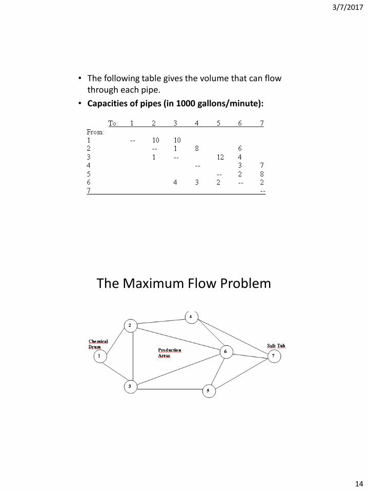
One production area contains a huge drum that holds up to 100,000 gallons of a poisonous chemical used in making various insecticides.

The drum is routinely filled to a level somewhere between 80,000 and 90,000 gallons.

• The flow of the chemical is then regulated through a series of pipes to production areas, where the chemical is mixed with other ingredients.

• There is a final section called disposal area, where the waste is deposited into a large “safe tub”.

• It is then collected from the safe tub and disposed of in a manner consistent with federal regulations.

3/7/2017

14

• The following table gives the volume that can flow through each pipe.

• Capacities of pipes (in 1000 gallons/minute):

The Maximum Flow Problem

3/7/2017

15

• The plan must determine which valves to open and shut, as well as provide an estimated time for total discharge of the poisonous chemicals into the secure waste area.

• The flow is possible in either direction between nodes 2 and 3, 3 and 6, 4 and 6, and 5 and 6. But, Flow is restricted to one direction for all other arcs.

• The problem can easily be formulated as a linear program.

• Xij represent the amount of flow between nodes i and j. (in 1000 gallons per minute).

The Objective is: Maximize X12 + X13

• The Constraints are as follows:

• The total flow out of source node 1 must equal the flow into terminal node 7:

X12 + X13 = X47 + X57 + X67

3/7/2017

16

• For nodes 2,3,4,5, and 6, The total flow into the node must equal the total flow out of the node:

• Node 2: X12 + X32 = X23 + X24 + X26 • Node 3: X13 + X23 + X63 =X32 + X35 + X36 • Node 4: X24 + X64 = X46 + X47 • Node 5: X35 + X65 = X56 + X57 • Node 6: X26 + X36 + X46 + X56=X63 + X64 +

X65 + X67

• The flows cannot exceed the arc capacities:

• X12 10; X13 10; X23 1; X24 8; X26 6; X32 1;

• X35 12; X36 4; X46 3; X47 7; X56 2; X57 8;

• X63 4; X64 3; X65 2; X67 2.

• The flows can not be negative:

• All Xij 0.

3/7/2017

17

• The problem was solved by using the Network Modeling option of WINQSB.

• The result is as follows:

From Node 1 to Node 2, The net flow is 7,000 gallons per minute.

From Node 1 to Node 3, The net flow is 10,000 gallons per minute.

From Node 2 to Node 4, The net flow is 7,000 gallons per minute.

From Node 3 to Node 5, The net flow is 8,000 gallons per minute.

From Node 3 to Node 6, The net flow is 2,000 gallons per minute.

From Node 4 to Node 7, The net flow is 7,000 gallons per minute.

From Node 5 to Node 7, The net flow is 8,000 gallons per minute.

From Node 6 to Node 7, The net flow is 2,000 gallons per minute.

Bagaimana solusi dengan Win Qsb

• The maximum total net flow From Node 1 to Node 7, is 17,000 gallons per minute.

• If the drum is full with 100,000 gallons, it will take about 100,000 / 17,000 = 5.88 minutes to empty the entire contents into the safe tub in an emergency situation.

3/7/2017

18

The TSP involves finding the minimum traveling cost for visiting a fixed set of customers. The vehicle must visit each customer exactly once and return to its point of origin also called depot. The objective function is the total cost of the tour.

Traveling Salesman Problem

2 3

1 4

5 3 5

2

3

2

1

3 2

4

4

The total number of solutions is (n-1)! /2 if the distances are symmetric. For example, if there are 50 customers to visit, the total number of solutions is 49!/2=3.04x1062.

3/7/2017

19

Traveling Salesman Problem

2 3

1 4

5

3 5

2

3

2

1

3 2

4

4

Solution

If the depot is located at node 1, then the optimal tour is 1-5-2-3-4-1 with total cost equal to 11.

Traveling Salesman Problem

Mathematical Programming

Inputs: n = number of customers including the depot cij = cost of traveling from customer i to j Decision variables:

otherwise0

. tocustomer from travels vehicle theif1 jixij

3/7/2017

20

Traveling Salesman Problem

jix

ix

jx

xc

ij

n

j

ij

n

i

ij

n

i

n

j

ijij

, allfor 0,1

allfor 1

allfor 1s.t.

min

1

1

1 1

(1)

(2)

Constraints (1) and (2) ensure that each customer is visited exactly once.

Traveling Salesman Problem

2 3

1 4

5 3 5

2

3

2

1

3 2

4

4

minimize 2x12+3x13+2x14+3x15+3x23+4x24+...+5x45

s.t. x12+x13+x14+x15 = 1 for node 1 x21+x31+x41+x51 = 1 for node 1 ... ...

3/7/2017

21

Traveling Salesman Problem

2 3

1 4

5

Is this solution feasible to our formulation? We need additional constraints, so-called subtour elimination constraints.

Traveling Salesman Problem

Si Sj

ij Sx subset every for 1

Si Sj

ij SSx subset every for 1

2 3

1 4

5

3/7/2017

22

Traveling Salesman Problem

Subtour elimination constraints for the example:

5,4,3,2,1 SS

2 3

1 4

5

1545324231413 xxxxxx

5,3,2,4,1 SS

1454342151312 xxxxxx

2 3

1 4

5

Traveling Salesman Problem

Heuristics for the TSP

1. Construction Heuristics build a feasible solution by adding a node to the

partial tour one at a time and stopping when a feasible solution is found.

Many construction heuristics are also called greedy

heuristics because they seek to maximize the improvement at each step.

3/7/2017

23

Traveling Salesman Problem

Nearest Neighbor

Step 1. Start with any node as the beginning of the path. Step 2. Find the node closest to the last node added to the path. Step 3. Repeat Step 2 until all nodes are contained in the path. Then, join the first and last nodes.

Traveling Salesman Problem

2 3

1 4

5 3

2 1

2

3

Start with node 2.

Nodes added Tour 2 2 5 2-5 1 2-5-1 4 2-5-1-4 3 2-5-1-4-3 2-5-1-4-3-2

2 3

1 4

5 3 5

2

3

2

1

3 2

4

4

3/7/2017

24

Traveling Salesman Problem

Nearest Insertion

Step 1. Start with a node i only. Step 2. Find node k such that cik is minimal and form subtour i–k–i. Step 3. Selection step. Given a subtour, find node k not in the subtour closest to any node in the subtour. Step 4. Insertion step. Find the arc (i,j) in the subtour which minimizes cik+ckj-cij. Insert k between i and j. Step 5. Go to step 3 unless we have a Hamiltonian cycle.

Traveling Salesman Problem

Farthest Insertion

Step 1. Start with a node i only. Step 2. Find node k such that cik is maximal and form subtour i–k–i. Step 3. Selection step. Given a subtour, find node k not in the subtour farthest from any node in the subtour. Step 4. Insertion step. Find the arc (i,j) in the subtour which minimizes cik+ckj-cij. Insert k between i and j. Step 5. Go to step 3 unless we have a Hamiltonian cycle.

3/7/2017

25

Traveling Salesman Problem

Arbitrary Insertion

Step 1. Start with a node i only. Step 2. Find node k such that cik is minimal and form subtour i–k–i. Step 3. Selection step. Arbitrarily select node k not in the subtour to enter the subtour. Step 4. Insertion step. Find the arc (i,j) in the subtour which minimizes cik+ckj-cij. Insert k between i and j. Step 5. Go to step 3 unless we have a Hamiltonian cycle.

Traveling Salesman Problem

Cheapest Insertion

Step 1. Start with a node i only. Step 2. Find node k such that cik is minimal and form subtour i–k–i. Step 3. Insertion step. Find arc (i,j) in the subtour and node k not, such that cik+ckj-cij is minimal and, then, insert k between i and j. Step 4. Go to step 3 unless we have a Hamiltonian cycle.

3/7/2017

26

Traveling Salesman Problem Clarke and Wright Savings Heuristic

1. Select any node as the central depot which is denoted as node 0. Form subtours i-0-i for i=1,2,...,n. (Each customer is visited by a separate vehicle)

2. Compute savings sij=c0i + c0j - cij for all i,j 3. Identify the node pair (i,j) that gives the highest saving sij

4. Form a new subtour by connecting (i,j) and deleting arcs (i,0) and (0, j) if the following conditions are satisfied

a) both node i and node j have to be directly accessible

from node 0 b) node i and node j are not in the same tour.

Traveling Salesman Problem

Clarke and Wright Savings Heuristic

5. Set sij=-, which means that this node pair is processed. Go to Step 3, unless we have a tour.

3/7/2017

27

Traveling Salesman Problem

Heuristics for the TSP

2. Improvement Heuristics begin with a feasible solution and successively improve

it by a sequence of exchanges while maintaining a feasible solution throughout the process.

Traveling Salesman Problem

Heuristics for the TSP

1 2

3 4

1 2

3 4

3/7/2017

28

Traveling Salesman Problem

Two exchange heuristics (2-opt)

Starting with any tour, we consider the effect of removing any two arcs in the tour and replacing them with the unique set of two arcs that form a different tour. If we find a tour with a lower cost than the current tour, the we use it as the new tour. When no possible exchange can produce a tour that is better than the current tour, we stop.

Traveling Salesman Problem

3 2 3

1 4

5 3 5

2 2

Suppose the initial tour is given as 1-2-3-4-5 with cost 15.

2 3

1 4

5 3 5

2

3

2

1

3 2

4

4

3/7/2017

29

Traveling Salesman Problem 3

2 3

1 4

5 3 5

2 2

3 2 3

1 4

5 3 5

2 2

Remove 1-2 and 3-4

Add 1-3 and 2-4 cost=18

3 2 3

1 4

5 3 5

4 3

Traveling Salesman Problem 3

2 3

1 4

5 3 5

2 2

3 2 3

1 4

5 3 5

2

Remove 1-2 and 4-5

Add 1-4 and 2-5 cost=11

3 2 3

1 4

5 3

2 1

2

3/7/2017

30

Traveling Salesman Problem

There are n (n-1)/2 - n possible ways of removing and adding arcs. In this case, n=5, and we have 5 combinations. The best tour obtained from the process at the first iteration is 2-3-4-1-5-2 with cost 11. We use this solution as the starting tour and apply the process again.

Contoh TSP; solusi dengan Win Qsb

Perusahaan “Q” akan menentukan rute terpendek perjalanan truk yang mengangkut teh botol pusat distribusi di CMH mengunjungi seluruh ritel dalam jaringan di bawah ini dan kembali lagi pusat distribusi di CMH.

3/7/2017

31

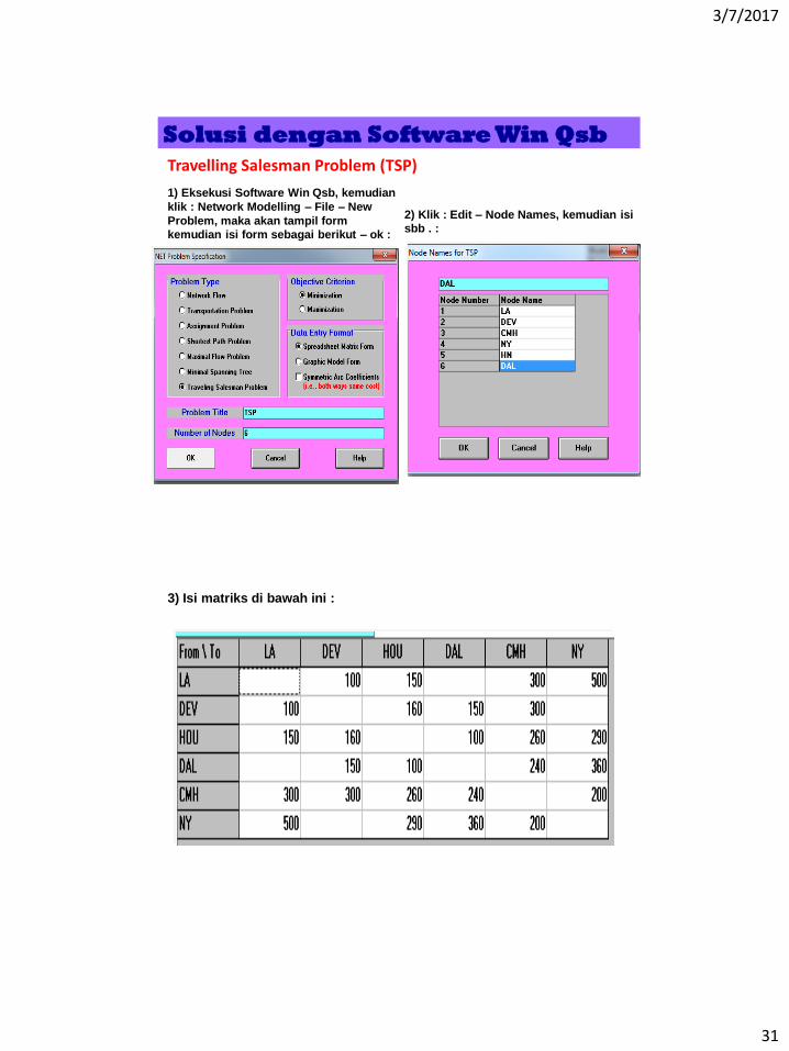
Solusi dengan Software Win Qsb

Travelling Salesman Problem (TSP)

2) Klik : Edit – Node Names, kemudian isi

sbb . :

1) Eksekusi Software Win Qsb, kemudian

klik : Network Modelling – File – New

Problem, maka akan tampil form

kemudian isi form sebagai berikut – ok :

3) Isi matriks di bawah ini :

3/7/2017

32

4) Klik solve and Analyze – solve :

5) Klik Result : Graphics Solution

3/7/2017

33

Model penugasan berguna untuk mengalokasikan pekerja-pekerja dengan skill tertentu pada mesin-mesin yang akan di-maintenance

Langkah – Langkah Penyelesaian (1)

1. Membuat suatu tabel biaya Opportuniti ( opportunity cost table ) yakni dengan membuat reduksi baris dan kolom

2. Buat tabel Reduksi baris : dengan cara mengurangkan semua biaya dalam tiap baris dengan biaya terkecil yang ada pada tiap baris tersebut.

3. Buat tabel reduksi kolom : dengan cara mengurangkan semua biaya yang ada pada semua kolom dari tabel reduksi baris dengan biaya terkecil yang ada pada tiap kolomnya

3/7/2017

34

Langkah – Langkah Penyelesaian (2)

4. Buat tabel biaya pengujian : yakni tambahkan garis pada tabel yang sudah direduksi baik secara vertikal maupun secara horisontal dimana terdapat minimal dua angka nol.

5. Untuk mencapai tabel yang optimal, maka jumlah minimal garis = jumlah baris atau kolom, jika belum maka buat tabel pengulangan model penugasan dengan cara kurangkan semua biaya yang tidak dilalui garis dengan biaya yang terkecil yang juga tidak dilalui garis dan untuk semua angka nol pada perpotongan garis harus ditambahkan dengan biaya yane terkecil. Kemudian tarik garis secara vertikal dan horisontal seperti langkah sebelumnya.

Langkah – Langkah Penyelesaian (3)

6. Apabila jumlah minimal garis = jumalah baris atau kolom, maka tabel tersebut sudah opitmal. Maka tentukanlah penugasan berdasarkan sel di mana terdapat angka nol.

3/7/2017

35

penggambaran umum:

mesin

1 2 . . . n

pekerjaan 1 2 . . . m

c11

c12

.

.

. cm1

c12

c22

.

.

. cm2

. . .

. . .

. . .

c1n

c2n

.

.

. cmn

1 1 . . . 1

1 1 . . . 1

model matematis:

0, jk pekerjaan ke-i tidak ditugaskanpd mesin ke-j

xij =

1, jk pekerjaan ke-i ditugaskan pada mesin ke-j

3/7/2017

36

model persoalan penugasan: n n

minimumkan: z = cij xij

i=1 j=1

berdasar pembatas: n

xij = 1, i = 1,2,…,n j=1 n

xij = 1, j = 1,2,…,n i=1

xij = 0 atau 1

jika pi dan qj merupakan konstanta pengurang thd baris i dan

kolom j, maka jika dilakukan operasi pengurangan pi dan qj thd

matriks ongkos, akan diperoleh “zero entries”, yaitu elemen-

elemen biaya dalam matriks yg berharga nol variabel-

variabel yang menghasilkan solusi optimum.

contoh:

mesin

1 2 3

Pekerja

1 5 7 9

1

2 14 10 12

1

3 15 13 16

1

1 1 1

3/7/2017

37

solusi awal

mesin

1 2 3

pekerjaan

1 5 7 9

1 1

2 14 10 12

1 1

3 15 13 16

1 1

1 1 1

Elemen-elemen nol dibuat dgn mengurangkan elemen terkecil masing-masing baris (kolom) dr baris (kolom) yang bersangkutan. Dengan demikian, matriks cij’ yg baru:

1 2 3

1

2

3

0

4

2

2

0

0

4

2

3

p1 = 5

p2 = 10

p3 = 13

Matriks terakhir dpt dibuat untuk memperbanyak elemen matriks yg

berharga nol dengan cara mengurangkan q3 = 2 dr kolom ke-3.

Hasilnya:

1 2 3

1

2

3

0

4

2

2

0

0

2

0

1

penugasan feasible dan optimum : (1,1), (2,3), dan (3,2)

biaya penugasan : 5 + 12 + 13 = 30

sama dengan p1 + p2 + p3 + q3 = 5 +10 + 13 + 2 = 30

3/7/2017

38

Seorang supervisor maintenance PTBA akan merencanakan penugasan 4 orang teknisi ke 8 mesin yang akan di-maintenance. Data nama teknisi, nama mesin dan estimasi waktu pengerjaan (jam) di masing-masing mesin adalah sebagai berikut : Keterangan: Data kosong = waktu untuk seorang teknisi yg. tidak memiliki skill untuk memaintenance mesin tersebut. AM1= jenis pekerjaan A untuk memaintenance Mesin1 (M1), dst…. Roni1=Roni2 = adalah orang yg. sama, hal ini dilakukan kr. software hanya mengalokasikan setiap inisial orang tepat kesatu jenis pekerjaan.

Buatlah rencana penugasannya, sehingga diperoleh total waktu pengerjaan paling minimum!

Eksekusi Win QSB, pilih Network Modelling – pilih Assigment Problem. Isi sebagai berikut :

Pilih Menu Edit - Node Names, kemudian edit nama pekerja dan nama mesin

3/7/2017

39

Entri, data waktu penyelesaian pekerjaan di masing-masing mesin sebagai berikut :

Klik menu Solve & Analyze – Solve Problem, maka akan tampil sbb. :

Untuk menampilkan gambar penugasan, klik Results – Graphics Solution

3/7/2017

40

3/7/2017

41

The Linear Programming Formulation

3/7/2017

42

3/7/2017

43

Transshipment or Transhipment is the shipment of goods or containers to an intermediate destination, and then from there to yet another destination. One possible reason is to change the means of transport during the journey (for example from ship transport to road transport), known as transloading. Another reason is to combine small shipments into a large shipment, dividing the large shipment at the other end. Transshipment usually takes place in transport hubs. Much international transshipment also takes place in designated customs areas, thus avoiding the need for customs checks or duties, otherwise a major hindrance for efficient transport.

Contoh :

Terdapat 2 buah pabrik dengan kapasitas supply masing-masing S1 = 600 dan S2 = 800. Untuk mendistribusdikan produk ke konsumen digunakan pusat distribusi (T), T1 membutuhkan 200 dan T4 membutuhkan 100 sedangkan T2 memiliki supply 350 dan T3 = 200. Retail di daerah pemasaran (D), membutuhkan D1 = 500, D2 = 350, D3 = 900. Biaya transportasi tertera di setiap busur.

3/7/2017

44

Matrix Transhipmentnya adalah sebagai berikut :

Bagaimana mendistribusikan barang dari pabrik melalui pusat distribusi untuk memenuhi kebutuhan pelanggan dengan total biaya transportasi minimum ? Gunakan Win Qsb untuk mecari solusinya.