3. windpro energy - institut for...

3.0 ENERGY – Intro, modules and step-by-step guide • 207

© EMD International A/S • www.emd.dk • WindPRO 2.4 • Jan. 04

3. WindPRO Energy 3.0 ENERGY – Intro, modules and step-by-step guide................................................. 209

3.0.1 Introduction to WindPRO energy calculation modules.........................................................................209 3.0.2 Step-by-step guide for energy calculation............................................................................................211

3.0.2.1 Based on measured data on site...................................................................................................211 3.0.2.2 Based on wind statistic and terrain description in simple terrain ..................................................211 3.0.2.3 Based on Wind Statistics and terrain description, complex ..........................................................211 3.0.2.4 Calculation of a Wind Statistics (WAsP required) .........................................................................211 3.0.2.5 Calculation of Wind Resource Map (WAsP required) ...................................................................211

3.1. ENERGY – Fundamentals in Calculations.............................................................. 213 3.1.1 Basic data for energy calculation .........................................................................................................213 3.1.2 Wind Speed Distribution.......................................................................................................................213

3.1.2.1 Methods for establishing a Wind Speed Distribution.....................................................................214 3.1.3 The Power Curve and the Ct Curve......................................................................................................216

3.2. ENERGY – Calculation Methods ............................................................................. 218 3.2.0 Introduction to calculation methods......................................................................................................218 3.2.1 Wind Atlas Method (ATLAS, WAsP and Resource).............................................................................218

3.2.1.1 Method description, ATLAS contra WAsP ....................................................................................218 3.2.1.2 Method description - the regional Wind Statistics .........................................................................219 3.2.1.3 Method description - Roughness Classification ............................................................................220 3.2.1.4 Method description - ATLAS Hills..................................................................................................224 3.2.1.5 Method description - ATLAS Local Obstacles...............................................................................225 3.2.1.6 Method description - WAsP Orography and Local Obstacles.......................................................226 3.2.1.7 Method description – RESOURCE................................................................................................226

3.2.2 Method description - Weibull and Measure..........................................................................................226 3.2.3 Method description - PARK (Wake loss calculations) ..........................................................................227

3.2.3.1 More than one wind data sets in a Wind Farm Calculation...........................................................228 3.2.4 Generating a Wind Atlas (a set of Wind Statistics) ..............................................................................228

3.3 ENERGY – Input data for WTG/Wind Farm calculation .......................................... 229 3.3.0 Introduction to data input for energy calculations.................................................................................229 3.3.1 Input for ATLAS or WAsP calculations.................................................................................................229

3.3.1.1 Siting and Setting Up Site Data Objects........................................................................................229 3.3.1.2 Tab sheet Wind Statistics (Wind Atlas) .........................................................................................231 3.3.1.3 Tab sheet Roughness in Site Data Object ....................................................................................232 3.3.1.4 Tab sheet ATLAS Hills/Obstacles in Site Data Object ..................................................................233 3.3.1.5 Tab sheet WAsP Orography/Obstacles ........................................................................................234 3.3.1.6 Tab sheet Map files and limits.......................................................................................................235 3.3.1.7 Input of WAsP obstacles ...............................................................................................................236

3.3.3 Input for a PARK-calculation ................................................................................................................236 3.4 ENERGY – Calculations and Printouts .................................................................... 237

3.4.1 Calculation ATLAS or WAsP interface (Energy, one spot) ..................................................................237 3.4.5 Printing and reading reports .................................................................................................................240

3.4.5.1 Printing ..........................................................................................................................................240 3.4.5.2 Reading reports from Energy calculations ....................................................................................241 3.4.5.3 Printing Data to file (Results to file) ...............................................................................................245

3.5 ENERGY - Uncertainty and Control.......................................................................... 247 3.5.0 Introduction to Uncertainty and Control................................................................................................247 3.5.1 Uncertainties.........................................................................................................................................247 3.5.2 Checking the Power Curve...................................................................................................................247 3.5.3 Verification by using existing WTGs.....................................................................................................249 3.5.4 Verification by using additional wind data ............................................................................................249

208 • 3.0 ENERGY – Intro, modules and step-by-step guide


3.5.4.0 Overview of the case studies and main specifications ................................................................. 250 3.5.4.1 Examples of wind data uncertainties ............................................................................................ 250 3.5.4.2 Verification by using more wind atlas for a large area.................................................................. 251



3.0 ENERGY – Intro, modules and step-by-step guide

3.0.1 Introduction to WindPRO energy calculation modules Calculating the Energy Production of a Wind Energy Project is one of the most important tasks of wind energy projecting. The annual energy production for a specific turbine can vary with several hundred percent depending on the micro siting, even within a small country like Denmark. Since the installation and operation costs usually are unaffected by the micro siting, the site dependent energy production becomes crucial for the feasibility of a wind energy project. WindPRO offers a range of options for calculating the energy production. WindPRO is the most flexible tool of its type when it comes to combinations of as well wind data in any format as WTG mix where as well mix of existing and new WTGs as different types and hub heights are treated flexible and intelligent. There has also been put a great effort into in the capabilities of getting intelligent check of as well data used in the calculations as the results order to invoke that the user get the most reliable results and documentation. At present, it is not possible to calculate the time dependent variations with the existing modules. Here, the user is referred to the Wind Energy Indices. Wind Energy Indices are available for more countries – ask EMD for more information. The module RESOURCE gives you access to establish a wind energy resource map, which gives you the information you need for selecting suitable sites – either on micro siting level for best positioning of the individual turbines, or for calculation of larger regions, where best suited sites for wind turbine projects are to be found. The module has special capabilities for calculating large areas in one process, and has been used for calculating the whole Denmark in a 200 m grid resolution. A wind resource map presented on screen on a background map is a valuable tool for manually optimizing a wind farm layout. For OPTIMIZING wind farm layout automatically, see separate chapter 8. For calculation with the Norwegian WindSIM CFD model, see separate chapter 9. The modules for energy calculation with WindPRO are: Three Modules, for "one spot" (single WTG) calculation or as basis for PARK-calculations (gives the wind data input to the array loss calculation for wind farm): ATLAS - With this module, you can calculate energy production based on simple ATLAS (Wind atlas method) model, based on terrain description (roughness, simple hills and obstacles) and a wind statistic. The roughness model is the same as in WAsP, but the hills and obstacles are calculated with more simple models as the flow model in WAsP. So ATLAS is only for non-complex terrain, and never recommended in mountainous terrain. Nevertheless the ATLAS model has been used for calculating more then 6.000 WTGs in Denmark which has worked quite good. METEO – With this module, you can calculate energy production based on measured wind data, where you have measured exactly where the WTG is going to operate from (in flat open terrain the data normally can be used for larger areas). If the measurements are taken in another height then proposed WTG hub height, the data can be extrapolated by giving in a wind gradient exponent, but this has to be used carefully. Only in flat and simple terrain (low roughness) the height conversion can be expected to follow simple rules. The METEO module will normally be more used for importing, analyzing and preparing measured wind data for generation of a wind statistic together with the WAsP interface. WAsP interface – With this module you can calculate the energy production using WAsP (software from RISOE, DK) as “calculation engine”, which means that you can calculate in complex terrain using the Wind atlas method with the advanced flow model incorporated in WAsP. WAsP interface is both a preprocessor to WAsP, for preparing and checking data and a post processor, for printing results in a nice report and for performing and printing a number of analyses, which gives the user valuable feed back for evaluating the quality of the calculation. Generating a wind statistic.



STATGEN – With the METEO and WAsP interface modules, measured wind data can be converted into wind statistics – the measured wind data are "cleaned" for local terrain conditions, so a regional wind climate is established for use in calculations on other spots than wind measurements is taken e.g. detailed calculation of a wind farm. Creating a Wind Resource Map. RESOURCE – This module can as "stand alone" make a presentation of a wind resource map based on a .rsf or a .wrg file from a WAsP calculation and e.g. a WTG size, if a WTG energy production map is wanted. Together with the WAsP interface module, the module can calculate the wind resource map, also for very large areas in one process. It can smoothly change the used wind data and automatically exchange digital maps for the WAsP calculation, which only can handle a limited size of map files in a resource calculation. Finally local obstacles can be included, and more hub heights calculated in one process. These features are not possible from a "pure" WAsP calculation of a resource map. The resource module also gives the "key" to operate module Optimizer based on .rsf files. Wind farm calculation. PARK is the module for calculating array losses and energy production for wind farms. The input for the PARK calculation is the WTG positions, types and hub heights, plus the wind data delivered from one of the 3 first mentioned modules (ATLAS, METEO or WAsP interface) OR from a .rsf file from the module RESOURCE. So to utilize PARK, one of the 4 mentioned modules must be available. Optimization of wind farm layout OPTIMIZE – Gives access to the PARK-design object, which is a useful tool for large-scale park design (e.g. off shore), which from ver. 2.4 can run a parameter variation for auto optimization. The other auto-energy optimizing algorithm is based on use in more complex terrain (see Chapter 8 Optimize). OPTIMIZE is based on the PARK module and RESOURCE module, and can only be used when these 2 modules are available.



3.0.2 Step-by-step guide for energy calculation

3.0.2.1 Based on measured data on site Establish map and proposed WTG project (see basis 2.0.5) Establish METEO object Input measured data in Meteo object – 4 levels of data input is possible: 1) Raw data logger files 2)

Time series from e.g. spread sheet 3) Table data (wind speed and wind direction frequency) or WAsP .TAB file, 4) Weibull parameters (or mean wind speed) versus direction sector (or just mean wind speed for preliminary calculations).

Run PARK (if wind farm) or METEO (if single WTG or site analyses, e.g. more different hub heights or WTG types). NOTE: Data has to be representative for long-term wind conditions. Measurements have to be in hub height or the wind shear known. Only for use on WTG positions more than 50 m away from mast if terrain is very simple (flat, without local obstacles or changing surface roughness). Otherwise, go to 3.0.2.4

3.0.2.2 Based on wind statistic and terrain description in simple terrain Establish map and proposed WTG project (see BASIS) Establish SITE DATA object for ATLAS calculation, select Wind Statistics (if not available, go to

Calculation of a Wind Statistics 3.0.2.4). Enter roughness rose (20 km radius), local obstacles and local simple hills – is done graphically from

“right click” options on site data object. Run PARK (if wind farm) or ATLAS (if single WTG or site analyses, e.g. more different hub heights or

WTG types)

3.0.2.3 Based on Wind Statistics and terrain description, complex Establish map and proposed WTG project (se basis) Establish height contour lines approx. 5 km radius around site in LINE object Establish roughness description in approx 20 km radius around site – 3 methods available: Roughness

rose (Site Data Object), Roughness lines (LINE object) or Roughness lines exported from the Area Object.

If local obstacles, establish these (Obstacle object). Establish a Site Data Object for WAsP calculation and select wind statistic (if not available, go to

Calculation of a wind statistic NOTE: A correct Wind Statistics is extremely important to calculate correct results). Check MAP data connected to the Site Data Object.

Run PARK (if wind farm) or WAsP interface (if single WTG or site analyses, e.g. wind profiles, more different hub heights or WTG types)

3.0.2.4 Calculation of a Wind Statistics (WAsP required) Establish map for measure mast site (see BASIS) Establish height contour lines approx 5 km radius around measure mast in the Line Object Establish roughness description in approx 20 km radius around measure mast – 3 methods available:

Roughness rose (Site Data Object), Roughness lines (Line Object) or Roughness lines exported from the Area Object.

If local obstacles, establish these (Obstacle Object). Establish a Site Data Object for STATGEN purpose and add data. Establish a Meteo Object – see 3.0.2.1 Run STATGEN from calculation menu (takes data from Meteo and Site Data Object.) Use Wind Statistic from 3.0.2.2 or 3.0.2.3.

3.0.2.5 Calculation of Wind Resource Map (WAsP required) Establish map and proposed WTG project (see BASIS) Establish height contour lines approx 5 km radius around calculation map area in the Line Object



Establish roughness description in approx 20 km radius around calculation map area – 2 methods available: Roughness lines (Line Object) or Roughness lines exported from the Are Object. From the Area Object, there can be imported information from e.g. .dxf files.

Establish a Site Data Object for RESGEN calculation; select Wind Statistics (if not available, go to “Create Wind Statistics”). Check MAP files and input region that you will calculate within.

Run a RESOURCE from calculation menu and set grid size, height(s) etc. Establish a Result Layer Object on map for presenting resource layer and for manually or

automatically optimization (module OPTIMIZE) of the wind farm layout.

3.1. ENERGY – Fundamentals in Calculations • 213

3.1. ENERGY – Fundamentals in Calculations

3.1.1 Basic data for energy calculation Two basic sets of data are needed in order for you to be able to estimate the annual energy production for a WTG: The wind speed distribution at hub height The power curve for the turbines If more WTGs are placed together and form a cluster or a wind farm, the directional Wind Speed Distribution, the precise micro siting of the WTGs and their Ct curve(s) must also be known.

3.1.2 Wind Speed Distribution The Wind Speed Distribution describes the probability for a specific wind speed versus the wind speed. The mathematical two-parameter Weibull distribution is often used to describe the Wind Speed Distribution. The next figure shows examples of measured distributions and corresponding Weibull curve fits.

The two Weibull distribution parameters are defined by:


214 • 3.1. ENERGY – Fundamentals in Calculations


u is the wind speed k is the Weibull form factor A is the Weibull scale parameter (for typical distributions, A ≈ is approx. equal to 1.126 * umean) A special variant of the Weibull Distribution is the Raleigh Distribution where k = 2. This distribution is often assumed when only the mean wind speed is known.

3.1.2.1 Methods for establishing a Wind Speed Distribution The Wind Speed Distribution can be established by one of the following methods:

A: Measurements at the WTG site B: One or more Wind Statistics for the region and a terrain description for the WTG site (simple terrain = Wind Atlas method, ATLAS)

C: One or more Wind Statistics for the region and a terrain description for the WTG site (complex terrain = Wind Atlas method, WAsP)

D: Measurements for the region (or on site, where more WTGs with different terrain conditions shall be sited), transformed to wind statistics for the region by WAsP (WindPRO module STATGEN). After establishment of a wind statistics, go to C:

A precise wind speed distribution is crucial. One reason for this is the fact that the energy content of the wind increases with the third power of the wind speed. The wind energy output from a WTG at a specific time is calculated with the following equation:

E = ½*ρ*w3*A*Ce (W/s) where: ρ is the Air Density w is the Wind Speed A is the Area Swept by the Rotor Ce is the total efficiency of the WTG at the given wind speed

An example: At the wind speed 10 m/s a 150 kW WTG with 23 m rotor diameter e.g. has an efficiency of 40% at air density 1,125. Then the energy is calculated as: E = ½ ·1.125 kg/m3 ·103 (m/s) 3· 232 · π/4 m2· 0.4 = 93434 W/s This means that the power is 93,4 kW and the energy production is 93,4 kWh in one hour. At half the wind speed, 5 m/s, assumed same WTG efficiency (which in practice will be lower), the power is 11,7 kW or only 12,5%. NOTE: The formula above cannot be used to calculate annual energy production based on the annual mean wind speed. The wind distribution and the power curve must both be known.



ad A. Measurements at the WTG site The measurements must correspond to the long-term wind conditions. Typically, this calls for continued measurements over a period of minimum three years. If at all possible, measurements of shorter periods must be controlled and correlated to the long-term measurements from a station within the same region. The data should be available in one of the following formats:

• Time series from data logger or spread sheet, normally with records of both wind speed and direction • Table/histogram with observations per wind speed interval (and normally by direction interval) • Weibull parameters, possibly given per wind direction sector • Mean wind speed, possibly given per wind direction sector

Data that is available in one of the above formats can be entered/imported in a METEO object in WindPRO. See also section 3.2.2 and 3.3.2

ad B. One or more Wind Statistics for the region and a terrain description for the WTG site (simple terrain) The wind speed distribution in relatively simple terrain can be calculated with ATLAS, e.g. as for most of Denmark (except those areas with large hill formations or industrial areas with many and dominating local obstacles). ATLAS requires a terrain data object and one or more wind statistics. The wind statistics should be based on measurements made within a radius of maximum 200 km from the site. See also section 2.1.x and 3.1.x

ad C. One or more regional wind statistics and a terrain description for the WTG site (complex terrain) For sites in more complex terrain, i.e. with many hills, mountainous terrain or terrain with dominating local obstacles, the calculation of the wind speed distribution can be carried out by using the energy calculation software WAsP. WindPRO calls WAsP (which must be purchased from RISOE) as the calculation module once a terrain data object has been created, WAsP selected as the calculation module, and one or more wind statistics have been selected. The wind statistics should be based on measurements made within a radius of maximum 100km from the site. Please notice that wind statistics in mountainous terrain may be valid within a very short distance (down to as little as a few hundred meters) from the measurement station. See also section 2.1.x and 3.1.x

ad D. Measurements for the region transformed into wind statistics for a region by WAsP and go to C The comments that were made under item A are valid here too. The only difference is that the data cannot be used directly, but has to be transformed into a set of regional wind statistics which are based on the measured data combined with a terrain description as outlined under item C. In other words, first a METEO object must be created in WindPRO, and then a terrain object for the measuring station must be created and used to generate a set of wind statistics for the measuring station (the regional wind statistics). The regional wind statistics can then be used as described under item B or C. See also section 3.2.1.

216 • 3.1. ENERGY – Fundamentals in Calculations


3.1.3 The Power Curve and the Ct Curve The power curve describes the electric power output from a specific WTG versus the wind speed at hub height. The power curve is typically measured by installing wind monitoring equipment close to a WTG, and measures the joint values of the wind speed and the electric power output. Alternatively, the power curve can be calculated using aerodynamic computer models. Power curves for a large number of the WTGs are already available in the wind turbine catalogue in the WindPRO BASIS module (WTG catalogue). The power curves are generally based on measurements or calculations. The reliability of the power curves may vary. Therefore, it is important to check the power curves. Please refer to Chapter 2.6 for further information on this subject. The Ct curve, which is used in PARK calculations, is usually just a standard curve for either stall regulated or pitch regulated WTGs. Experience indicates that this is sufficient, but more detailed scientific work on the subject is lacking.



Further information about the power curves can be found in the chapter 2.6 in WindPRO BASIS. A typical example of power curve, Ce and Ct curves for a stall regulated 2-speed generator WTG are displayed in the above figures.

218 • 3.2. ENERGY – Calculation Methods


3.2. ENERGY – Calculation Methods

3.2.0 Introduction to calculation methods In this chapter you will find a short description of the various calculation methods that can be used from WindPRO. The following methods will be described: • Wind atlas method (module: ATLAS, WAsP interface and RESOURCE) • Direct use of measurements (module: METEO with Weibull or measure option) • PARK - this calculation is used in conjunction with one of the methods mentioned above. Note that also export of data for the Norwegian WindSIM CFD model (preprocessor) as well as a post-processing module is available. See separate main chapter 9 in manual for further details.

3.2.1 Wind Atlas Method (ATLAS, WAsP and Resource) All calculations methods are based on the wind atlas method. The wind atlas method presupposes that you use a set of wind statistics for a specific area (the local wind atlas). Combined with a terrain assessment of the area within 20 km radius around the site, the program calculates the actual mean site-specific wind conditions at any specified height above the site terrain. These wind data can then be compared with the power curve of a specific WTG, after which the expected mean annual energy production for that WTG at the chosen site can be calculated. Hence, three sets of information are required for an energy production calculation based on the wind atlas method:

• The governing wind statistics for the region • A terrain assessment (roughness, orography and local obstacles) • Power curves for the WTG (s) in question

3.2.1.1 Method description, ATLAS contra WAsP The WindPRO program module ATLAS complies with the algorithms that are described in the “European Wind Atlas” with the following limitations:

• Only one obstacle per wind direction sector can be entered. Also, the obstacle model is simplified compared to the WAsP model.

• The hill model is simplified and is not based on a flow model, as the WAsP model. The hill model is based on a simple mathematical model, which only calculates with the height and the length of one hill in each directional sector.

• The stability model, which is described in the “European Wind Atlas” and which adjust the wind profile at sites within 10 km from a coastal line, is not included in the ATLAS program. However, sensitivity analyses carried out by EMD indicate that only marginal errors may occur if the stability model is not included.

One of the key elements in the wind atlas method is the terrain assessment. The terrain must be described via the following:

• Roughness classification of the terrain - detailed within 5 km from the site, coarser within 20 km from the site.

• Hills (orography) at the site - in a radius of approx. 5 km if you use digital maps. • Local obstacles within about 1000 m from the WTG position.

Usually, a terrain assessment requires both good maps and a field survey.

3.2. ENERGY – Calculation Methods • 219


3.2.1.2 Method description - the regional Wind Statistics The governing regional wind statistics (wind atlases) for most of the European countries (1989) are mapped in the “European Wind Atlas” from Risoe. A number of other countries, e.g. the new EEC members Sweden and Finland, have made similar mappings. It is not possible to explicitly point out exactly which wind atlas to use for a specific site (in Denmark, one should generally choose DANMARK ‘92). But one should generally use a Wind Atlas, which is based on the measuring station closest to the site, and then control the result by comparing the result with wind statistics from one or two adjacent measuring stations. Another approach would be to specify a number of wind atlases in the same calculation, weighted by the reciprocal distance to the site. The regional wind atlas constitutes a complete description of the governing wind conditions for the region in question, and consists of a table that contains the following default WAsP setup. The parameters can be changed manually in the WAsP parameter file: Weibull A and k parameters for: each of the roughness classes 0, 1, 2, 3 (4 in total) each of the heights 10, 25, 50, 100, 200m above ground level (5 in total) each of the directions N, NNE, ENE, E, ..., NNW (12 in total) This gives a total of 4*5*12 = 240 wind speed distributions The most critical aspect of the wind atlases is their quality, which may vary significantly. An error margin of 50% in the estimated energy production is easily generated simply due to the fact that a wind atlas of poor quality was used. It is therefore important to crosscheck the applied wind atlas with other “neighboring” wind atlases, and preferably make test calculations for other WTGs in the region, which have been operating for some years.

Recommendations for Site Calculations in Denmark When calculating the wind energy potential for sites in Denmark, the “Danmark ‘92” wind atlas is recommended. It includes a set of correction curves that enable you to scale the production according to the geographical position (the correction for differences in the geostrophic wind conditions (~1000m agl.) over Denmark is based on comprehensive studies and production controls for a large number of Danish WTGs). The map below (EMD/InterCon I/S) shows which correction factor one should use on the calculated production when one uses the “Danmark ‘92” wind atlas (which, by the way, is identical with the “Beldringe” wind atlas included in the European Wind Atlas).



Recommendations for Site Calculations outside Denmark In general, the data from the European Wind Atlas seem reliable. When other wind statistics are used, it is recommended always to include at least two wind statistics from the region, and make sure that the differences between these data are acceptable - or to include the production from existing WTGs as control elements in the calculation. WindPRO can work simultaneously with several wind atlases. The program automatically calculates weighting factors for the individual wind atlases proportional to their reciprocal distances to the site. These factors can, if needed, be edited afterwards based on more detailed information. If, e.g., the site is placed in a coastal area, it would often be more correct to give coastal wind statistics a higher weighting - even if closer inland statistics are available. The use of several wind statistics in the same calculation can reduce the uncertainty factor. See also chapter 3.5 regarding (quality) control of data.

3.2.1.3 Method description - Roughness Classification Roughness classification can be performed in 3 different ways:

Roughness rose: Description from site for each separate sector (one or more “belts” per sector). B. Digitizing a roughness line map (line object) C. Export of roughness lines from “land use” polygons. Land use polygons can be digitized withthe AREA object or imported into same object from other information sources.

The ways of using the 3 different methods are made very comfortable with the WindPRO software. For B, a line object must be used, for C, an area object must be used - this is described in WindPRO manual chapter 2, BASIS. In the following the most important, how to classify roughness, is described with start in method A: The terrain is divided into 8, 12 or more sectors depending on the available wind statistics. Most of the wind statistics available today are specified in 12 30-degree sectors with the following center angles:


0 degree: (345 degrees to 15 degrees) (N) 30 degrees: (15 degrees to 45 degrees) (NNE) 60 degrees: (45 degrees to 75 degrees) (ENE) 90 degrees: (75 degrees to 105 degrees) (E) Etc.

The roughness of the terrain should be described for each sector in a distance of at least 10 km from the site. Depending on the hub height and terrain conditions, a longer distance may be relevant. It is, however, recommended to use this distance in every terrain description. It is possible to include up to 10 roughness changes in each sector in case the terrain changes its character with the distance from the WTG. In the following figure, the impact of a roughness change at different distances from the WTG is illustrated.

The above figure illustrates as an example that with an inner roughness class = 3 and an outer roughness class = 0; and a change in 3000 meter distance; 72% of the production will be determined by the inner roughness class when the hub height is 30m, while only 50% of the production will be determined by the inner roughness when the hub height is 60m. You can choose to use either roughness classes or roughness lengths (see next table).




In areas with hedges, following figure can be used to estimate the roughness class/length. The figure displays a number of graphs designed to help you to determine the roughness class/length of an area with hedges. Notice the non-linear impact of the hedge height on the roughness class. Normal farming land is assumed to lie between the hedges, and this has been included in the figure by adding 0.03 m to all specified roughness lengths. A porosity of 0.33 is assumed.


In an area with many buildings, the roughness length can be estimated via the following equation:

z0 = 0,5 * h2 * b * n / A where: h = height of building b = width of building n = number of buildings A = total area within which the n buildings are situated

NOTICE: The roughness length of the area between the buildings must be added to the roughness length which has been determined on the basis of the above equation 3.1, e.g. add 0.03 m to the calculated roughness length for normal farm land. The correlation between roughness classes and roughness lengths is indicated in the next figure.




If a sector between two roughness changes consists of more than one roughness class, a simple weighting of the roughness classes in the area is recommended. If, for example, the area consists of: 2/4 Roughness Class 2, ¼ Roughness Class 1 and ¼ Roughness Class 3, the resulting Roughness Class becomes: (2*2 + 1*1 + 1*3)/4 = 2. It is important that a roughness classification covers an entire roughness area/belt, i.e. a roughness belt with a width 1000m with one crossing hedge of 10 m heights should be assessed to the roughness class 2. It is often seen that such an area has been classified as roughness class 1 all the way to the hedge, with a shift to roughness class 3 for a few meters along the width of the hedge, and with a final roughness class of 1 just after the hedge. This is incorrect! The “European Wind Atlas” recommends doubling the width of every new roughness belt when moving outwards from the WTG. Another important rule: Even if an area is located at a ground level which lies lower than the turbine site, the roughness classification is not affected by this fact. The differences in terrain heights are included via the hill model! In practice, visiting the site and making preliminary notes regarding the roughness classes and the distances between the roughness changes carry out a terrain assessment. Furthermore, notes are taken regarding local obstacles and their dimensions. Having completed the site visit, the exact distances between the roughness changes and the final design of the roughness classifications are determined at your desk by using the map and the above-mentioned tools. However, much of the measuring work can be avoided by using digital background maps in WindPRO (see the below description of this feature). It is important that you carry the map with you when you visit the site. It allows you to verify the map signatures and evaluate the size and porosity of the local obstacles.

3.2.1.4 Method description - ATLAS Hills By siting the WTG on the top of a hill you will usually be able to exploit the above-mentioned increase of the wind speed. During the visit to the site it is necessary to judge whether or not the streamlines of the wind flow will be compressed at hub height and result in an increase of the wind speeds there. The same theory applies in a negative sense, if the WTG is placed on the lee side of a hill. If the terrain is very complex, e.g. mountainous, an analysis using WAsP should be considered (see the description of this feature in the next chapter).


In the ATLAS model, a simple numerical calculation of the hill influence is carried out on the basis of information about the sector wise hill length (the length from the WTG to the hill base) and hill height. One set of data can be entered in each of the usually 12 sectors.

In the above figure you can see how Hills usually increase the wind speed because of the compressed streamlines (the same amount of air per time unit passes through a reduced cross section resulting in higher wind speeds). Cliffs and other abrupt orography changes should not be included when using the hill model, as there is no method available today which allows you to calculate the effects of such orography changes. Great precaution should be taken when siting WTGs close to cliffs or other abrupt orography changes.

To illustrate the influence of siting a WTG on a hill, the above figure show the production increase for a WTG situated on a hill with a circular base. Please notice that even for very small hill radii, the model changes so that it calculates the influence from the hill as if the hub height had been increased instead. If one used the mathematical model from “Vindatlas for Danmark” the calculation would result in a negative change in the wind speed.

3.2.1.5 Method description - ATLAS Local Obstacles Single obstacles, e.g. buildings, hedges etc.(of more than ¼ of the hub height) near the WTG (within approx. 1000 m of the turbines) should be treated as local obstacles and not as roughness elements.




An obstacle is measured by eye during the site visit and the accuracy of this measurement is purely based on the experience of the person. The exact distances are later on found by calculating the distances on the map. If the obstacle is lower than ¼ of the hub height or farther than 1000 m away it should not be included in the calculation as an obstacle, as it will exert no or only marginal influence on the calculation result. However, it has to be included as a roughness element in the roughness classification! Aside from the geometrical dimensions of the obstacle, also the porosity of it has to be judged. The following figure shows how the program handles obstacles.

3.2.1.6 Method description - WAsP Orography and Local Obstacles The WAsP program from RISOE can be used as the calculation model from the WindPRO module WAsP interface. Here hills and local obstacles are calculated by means of a flow model. This requires a much more detailed description than the more simple ATLAS model. Hills are described through digital height contour maps. Local obstacles are described as rectangular boxes. More local obstacles can be distributed freely in the same sector, and both the rotation and the depth of the local obstacle can be set (see the WAsP user’s manual for further details).

3.2.1.7 Method description – RESOURCE Resource is just WAsP calculations performed automatically for a grid. The advantage of the resource module in WindPRO relative to directly use of the WAsP software is that WindPRO offers to include local obstacles and to use more different wind statistics in same calculation, so the wind climate smoothly can be changed from one part of the calculated grid to another.

3.2.2 Method description - Weibull and Measure When calculating with module METEO, two different options is offered: Weibull and measure. The difference is that choosing the measure option means that the "raw" table values in meteo object is used instead of the Weibull data (normally this is best Weibull fit of the METEO table values). If measured data for a representative period (see section 1.1) are available for the actual site the energy production can be calculated by simply integrating the bin-separated products of the wind speed distribution and the power curve.


Please notice that the program will automatically convert measurements, which have been made at another height but the hub height, into hub height data based on the entered wind gradient exponent by means of the below equation:

Where γ is the wind gradient exponent. Conversions over major height differences (more than 20-30%) are connected with large uncertainties. The following general guidelines can be used if the wind gradient is not known. These guidelines are based on data from “Vindatlas for Danmark”, and are not necessarily applicable worldwide - especially in complex terrain (or just simple hills) one should not rely on these guidelines for any conversions other than marginal height differences.

If only one set of Weibull parameters are available, an average wind gradient exponent should be specified. You could e.g. use a weighting based on the distribution of wind directions. When wind data are available as frequencies that have been sorted into wind speed intervals (a histogram), it is optional to use the data directly or to use a Weibull curve fit. The later choice is usually recommended, as the curve fitting procedure will filter the measured data and the effect of outliers reduced/eliminated. The Weibull fit follows the procedure specified in the “European Wind Atlas”, where low wind speed frequencies are weighted with lower values than wind speed frequencies within the normal operation range of the WTGs.

3.2.3 Method description - PARK (Wake loss calculations) The PARK module calculates the wake losses due to the shadowing effects between WTGs sited close to each other (Wind Farms and Clusters). The method follows the model that was created by N.O.Jensen from RISØ, but with small modifications that enables one to work with different WTG types and Hub Heights in the same layout. The basic equation for calculating the wake loss behind a rotor is:

Where v is the wind speed at a distance x behind of the rotor u is the free wind speed just upstream from the rotor R is the rotor radius α is the wake decay constant.




2/3 is an approximation value of the Ct value – in calculation model; the “real” Ct value is used for each wind speed interval.

The figure below shows the basic idea behind the simplified wake model for wake losses behind a turbine. The wake decay constant is a measure for the down stream widening of the “shadow cone” behind the wind turbines. The constant is specified as widening in meters per meter downstream of the rotor. A constant of 0.075 m, corresponding to an opening angle of approx. 4 degrees is usually recommended.

Measurements that Risoe has carried out on different wind farms indicate that the wake decay constant depends on the turbulence and therefore on the roughness class - varying from 0.04 for a roughness class 0 to 0.1 for a Roughness Class 3. The use of the default value of 0.075 for all calculations on land is judged to have only marginal impact on the results. Offshore the value 0.04 should always be chosen. NOTE: For very large wind farms (>50 WTGs) some newer measurements indicates that the PARK model might not treat the array loss calculation well – the wind farm itself changes the roughness, and the "supply" of new wind inside a large wind farm might not follow the assumptions in the N. O. Jensen PARK-model. This might lead to an improved PARK model in the near future.

3.2.3.1 More than one wind data sets in a Wind Farm Calculation When carrying out a PARK calculation, one must always judge whether one overall wind speed distribution represents the site conditions correctly, or if several terrain descriptions or measured sets of data are needed for an accurate calculation of the entire park layout. No guidelines can be specified, as the choice will depend on the complexity of the terrain, the size of the wind farm and the required accuracy. If more than one set of data is specified, PARK will always use the data set closest to the individual WTG in the calculation. Another way to get individual calculated wind distribution for each WTG in a wind farm is using A with link to digitized roughness and height contour lines.

3.2.4 Generating a Wind Atlas (a set of Wind Statistics) If measured wind data are available for the site or for the region in question (within maximum approx. 100 km from the site depending on complexity of the terrain) you can choose to generate a regional wind atlas that can be used for both ATLAS and WAsP calculations as described in section 3.2.1.2 This requires that the WAsP program is installed on the hard disk, and that you are familiar with processing wind data. The modules METEO and WAsP interface gives automatically access to the use of the STATGEN module for generating wind statistics. Besides generating wind atlases WindPRO can also import wind atlases that have been generated in WAsP (.lib files) (see the WAsP manual for further information).

3.3 ENERGY – Input data for WTG/Wind Farm calculation • 229

3.3 ENERGY – Input data for WTG/Wind Farm calculation

3.3.0 Introduction to data input for energy calculations In the following, the procedures for entering the necessary information for performing calculations in WindPRO are described. See also step-by-step guide, 3.0.2. Please first refer to the WindPRO BASIS description on how to create the basic project, before entering into the specific data for energy calculation. The objects, which can be entered specific for the energy calculation, are listed below:

Site data object – ATLAS and WAsP interface (and RESOURCE, see also 3.6).

Meteo object - Weibull and measure.

A wind statistics (wind atlas or .LIB file) can be generated when having both site data object and METEO object and WAsP. PARK calculation (array loss calculation) can be performed based on site data object, a METEO object or a wind resource file (.rsf file).

WAsP Local Obstacles - NB! Has no effect in an ATLAS Calculation! The other relevant objects, described in chapter 2 Basis are:

New WTG

Existing WTG

Line object (both for height contour lines and roughness lines)

Area object (for polygon roughness areas – must be exported to lines)

Result layer – for presentation of wind resource map on screen.

3.3.1 Input for ATLAS or WAsP calculations You enter the information for ATLAS and WAsP calculations simultaneously. If you do not have the WAsP program you just skip the items referring to this program module.

3.3.1.1 Siting and Setting Up Site Data Objects A site data object can be created by:

• Select the object from the toolbar • Position it on the map at the position for the terrain assessment • With a mouse click it is established and the input form appear

Positioning the site data object will normally be in the middle of the wind farm. But please read the following carefully:


230 • 3.3 ENERGY – Input data for WTG/Wind Farm calculation


If roughness rose is used as roughness description method, all WTGs in a wind farm will be calculated with the exact same roughness description. To compensate for this, you can add more site data objects and thereby specify different roughness roses. Each WTG in the wind farm will then select the NEAREST roughness description. The same goes for obstacles and hills, if the simple ATLAS model is used. If you use roughness lines (only when using WAsP) all WTGs in a wind farm will be designated an INDIVIDUAL roughness description. Using height contour lines (only when using WAsP), each WTG in a wind farm is calculated individually with respect to orography. Once the site data object(s) has been created, a window appears where the use of the object is to be defined.

About coordinates, description, labels, layers etc., se chapter 2.5 Basis. Note: z-coordinate has no influence on the calculation and can be omitted here. If WAsP is installed and linked to WindPRO you can choose to use the terrain data object in the ATLAS module or the WAsP module exclusively, or in both modules. In the last case, you have to specify the model during the calculation. Another option is to use the terrain data to generate a wind statistics (see chapter 3.3.4) or to calculate a wind resource map (see chapter 3.6). The selection of the above calculations determines which data you can enter on the following tab sheets. ATLAS and WAsP have a simple and a detailed terrain description of the hill and local obstacles conditions respectively. STATGEN and RESGEN can only work with the more detailed WAsP data formats. Depending of the use, the object will change color on the map. The colors are:

Black – for Atlas Blue – for WAsP Cyan – for both Atlas and WAsP Orange – for STATGEN Green – for RESGEN


3.3.1.2 Tab sheet Wind Statistics (Wind Atlas)

One or more wind statistics can be selected for the same calculation. The “Edit wind statistics” button leads to a maintenance window, where e.g. .LIB files can be imported and given coordinates, which means that they will appear on the map shown in the selection window.

When “select wind statistic” is chosen, there are several optional search filters available. If no country or source has been marked then all wind atlases will be shown. Note: You can click on more countries, sources etc. NB: For calculations in Denmark the “Danmark ‘92” Wind Atlas should always be selected due to its special status. Regional correction curves have been linked to the wind atlas based on comprehensive investigations of a large number of Danish WTGs. Therefore, this wind atlas is judged to be significantly more accurate than other available wind atlases. Note: One of the most important things in an energy calculation is to evaluate the energy "level" of the wind statistic. There are so many possibilities for mistakes, that a final evaluation of the energy level by comparison with the level for statistics in the region might be the way to discover fatal mistakes. From the wind statistics selection window both the absolute as well as the power curve-filtered power curve level is shown, as a percentage compared the Beldringe wind statistics (Middle of Denmark).




3.3.1.3 Tab sheet Roughness in Site Data Object

The Roughness Classification can be entered directly, if you do not have a digital map or if you have already received the roughness classification from another source. The input tab sheet shows the input fields for the roughness classification, i.e. enter the information for one sector at a time and shift to a new sector by double clicking on <return>. Furthermore, you can import and edit digital roughness maps (from WAsP .MAP file) or read .RDS (WAsP roughness description) files from previous WAsP calculations (see the below explanation). One of the very strong facilities in WindPRO is, the possibility of creating and editing a roughness classification directly on the digital map. Two other possibilities are: Link to file – define the roughness line file in tab sheet “Map files and limits”. Link to line objects – automatically use line objects in your project with roughness lines. Both possibilities have the advantage, that each WTG in a wind farm will get an individual roughness classification. About changing between roughness class and length, note that moving the button, KEEP the values (should only be used, if by accidence there has been typed classes when setup was lengths). If conversion is wanted, press the convert button.

On screen roughness classification by roughness rose


When the map has been fetched and is rendered on the screen, you can drag the map by pushing the “hand” around while pressing on the left mouse button. If the roughness rose is activated you gain access to the below features by clicking on the right mouse button:

• Roughness - the roughness class is selected from the table for the area where the cursor was placed when you clicked on the right mouse button.

• Edit roughness - option for entering actual roughness classes. • Create change - creates roughness changes in the area that was activated by the cursor when you

clicked on the right mouse button. • Delete change - erases the roughness change closest to the cursor in the direction of the roughness

rose center. • Properties - activates the input window for the terrain data object. • Delete - erases the site data object. • Options - changes the setup for the size of the automatic roughness step size when they are moved. • Deactivate/Activate - changes the status for the actual terrain data object so that only its position is

marked. This option is useful when entering other objects, including other terrain data objects. • ATLAS hills and obstacles - shifts the object status from input of roughness to input of hills and local

obstacles (see the next section). Please notice that the roughness change lines can be dragged around by holding down the left mouse button when the cursor is positioned on a line.

3.3.1.4 Tab sheet ATLAS Hills/Obstacles in Site Data Object As for the roughness classification, both hills and local obstacles can be entered either via the object list or directly on a digital background map. Please refer to the previous section for information on how to activate the graphic input menu. For each sector it is possible to create one hill and one local obstacle.




The program automatically calculates the distance from the center of the site data object to the hill base/local obstacle and the obstacle width/width in sector. The objects can be dragged to desired positions with the mouse when it is activated. The hill height (difference from base to top) and the obstacle height and porosity must be entered in a table (select this option by clicking on the right mouse button under “Properties”). Please notice, that entering the elevation of the hill base can also enter the hill height. To use this method it is necessary to enter the z-coordinate for the terrain data object under the tab sheet “Position”.

3.3.1.5 Tab sheet WAsP Orography/Obstacles

If WAsP is chosen as the calculation module it is possible to use digital maps with height contours (digital orography maps) and local obstacles in WAsP format. If you “link to Line Objects”, one or more line objects with height contour lines, which are marked “for use in energy calculation”, automatically will be used. See the check box in the bottom of line object properties shown below.


If digitized height contour line maps only exist in files (not loaded into line objects), it is possible to link them, se next section. Once a series of local obstacles has been created, (see section 3.3.1.7), it is possible to define which of the local obstacles that are to be included in the calculations via the site data object menu. Then only those obstacles, which are situated within the radius of the individual WTGs, will be included in the calculation.

3.3.1.6 Tab sheet Map files and limits If there are no height or roughness data established in line objects, but the data exists in files, these files must be added to the site data object map list before they will be included in the energy calculation.

In the example above, roughness is included as a .map file, and orography is included in the list as a line object. BOTH a Line Object and a .map file which holds both roughness and orography lines. Here the data from line object will be used, because this is decided in the WAsP orography/obstacle tab sheet. Once the .MAP files have been selected, it is possible to define the area of the .MAP files that is to be included in the calculations, or to define a radius around each of the WTGs that are to be included in the calculations. The indicator “Maximum points” shows the number of digital points which are included in the boundary file and which will be calculated. This information is important when working with the older DOS WAsP version 4 as this version only can handle up to 10 000 points. BigWAsP 4 can handle up to 16 000 points. The WAsP version 5.0 can handle around 150 000 points, while WAsP 7 can handle approx. 250 000 points and WAsP 8 approx. 500.000 points (in one file).




Note, the “Map limit” window in the lower right part of screen dump in the above figure. This shows the position and size of the maps relatively to the project. This is an important check of whether the maps cover an appropriate size and if the maps are in the right coordinate system. If not, it will be easy to see in the map limit window.

3.3.1.7 Input of WAsP obstacles

Local Obstacles are created on a background map with the WAsP Obstacles icon. Here, the dimensions are defined by dragging the corners of the object to the desired size. When the object has been positioned, the following window appears where you can enter height and porosity:

Porosity decides how much wind that passes trough the obstacle seen as an average during the seasons.

3.3.3 Input for a PARK-calculation To perform an ATLAS or WAsP calculation it is not necessary to create WTGs as objects but during the calculation you can choose which WTGs and hub heights to calculate. However, when performing a PARK-calculation it is necessary to enter the WTGs on the map, as it is their inter-placement and WTG-type that is essential for the PARK-calculation. If the wind farm has a certain extension it might be relevant to use several site data or Meteo objects. Each turbine will then use the nearest object (but only from the selected ones in calculation setup –as default all are selected). Using digital roughness and height contour lines are the best methods. Using a WAsP-calculation for each WTG in the park will calculate the effect of the orography and local obstacles individually. To calculate the roughness classification individually it is necessary to attach a digital roughness map produced by means of WAsP. If you have created combined ATLAS- and WAsP site data objects the PARK-calculation will always choose a WAsP-calculation. However, if you want to use the ATLAS-calculation as a background to the PARK-calculation it is necessary to change the setting of the site data object only to use an ATLAS-calculation. Details on how to input the more specific parameters for a PARK calculation is described in 3.4.3

3.4 ENERGY – Calculations and Printouts • 237

3.4 ENERGY – Calculations and Printouts

When all the objects have been created, you can return to the WindPRO main menu, e.g. by clicking on the calculation tree icon.

A calculation is started by clicking on the green button (arrow) beside the required calculation. NOTE: Modules to which you have no license will be marked with a yellow button indicating that these will only run in a DEMO mode, i.e. calculations will use standard values and not the actual values entered. Note: The RESOURCE Module is described separately in chapter 3.6.

3.4.1 Calculation ATLAS or WAsP interface (Energy, one spot) Depending of which "use of object" you have given in your Site Data Object, one of the below two can be chosen: ATLAS WAsP interface


238 • 3.4 ENERGY – Calculations and Printouts


On the first tab sheet “Main” you can enter the hub height for key results. The program then calculates the mean wind speed, the energy and the equivalent roughness class for this height at the position where the site data object is placed. You can specify an uncertainty percentage under the “decrease option”. The main result and the result reduced by the uncertainty percentage will be shown on the results printout. Air density can be entered as height and annual mean temperature. Air density is IMPORTANT, because a low air density (high altitude or high temperature) reduces the energy production remarkable.

Note, that a wind profile can be calculated from the ATLAS or WAsP interface calculation (not from PARK, later described). Note, the button “Edit WAsP parameters” – this is only for “experts” in the use of WAsP. (Appears only when WAsP interface is chosen).


You select the objects to be used in the calculations on the second tab sheet: Wind distribution and WTGs. Calculation can include different WTG types and hub heights in the same calculation. The list of WTGs can be entered with default information about the WTGs that have been created as objects. Other WTGs can be added from the WTG Catalog.




3.4.5 Printing and reading reports

3.4.5.1 Printing

After the calculation has been completed, the above window will appear listing the available reports that can be printed. ‘Status’ shows the number of pages that will be printed if the actual report is to be printed with default settings. The status indicators will turn green if the calculation is OK and a red if the assumptions (input data) for the calculation have changed after the calculation was completed. A red cross in front of a calculation indicates that the data, which the calculation was based on no longer, exists. However, the report can still be printed. Please notice that a “sub report” will automatically pop up on the screen if you double click a sub-report name and that a sub report has its own “right click” options. When you right click the calculation header or one of the calculation reports, you gain access to the following features:

Properties: Edit calculation setup for recalculating (or view calculation setup). Calculate: Recalculate (used e.g. if positions of WTG is changed, but the calculation setup is unaltered). Print: Show the print options with the possibility of making changes (e.g. map scaling). Stop: To stop a running calculation. Copy: Make a copy of the calculation – useful, if a calculation based on changed object information is required with the present calculation setup, without overwriting the former calculation. Delete: Removes actual calculation report. Rename: For changing calculation name, description and uncertainty reduction percentage without recalculating Result to file: Makes it possible to save results to a file or copy to clipboard.


From “Print” option, following screen appear:

Note, that there are a large number of possibilities for change of print options. Select a report, and watch how the right part of the screen offers you different set up facilities. Remark: The object settings (label size etc.) can only be changed, when the report “Map” is selected. For more details on printing reports, se chapter 2 Basis.

3.4.5.2 Reading reports from Energy calculations Examples of reports are given in chapter 1. Below a few sample parts of the reports will be shown and some of the key figures will be explained.

The assumptions for the energy calculation concerning chosen wind statistic(s), air density and Wake Decay Constant is shown.

Key results are based in the position where the site data object(s) is placed and for the hub height chosen in the calculation set-up. The Equivalent roughness is the roughness class in flat terrain with no obstacles that would give the same calculated energy production. This can vary with the chosen hub height for key results if there are obstacles or orography, while the reduction/speed up from obstacles/orography vary with height.




Above the “most complex” presentation, where both new WTGs and existing PARK WTGs (marked as PARK WTGs in object with existing WTGs) are present in the calculation. Here results are given for as well the complete Windfarm production as the New only (including array losses from existing) and the existing both with and without the new WTGs. The column with withdraw of xx% is controlled by the user when setting up calculation. Wind farm efficiency is a measure of how much each single turbine produces – taking the array losses into account - relatively to the unreduced production. Capacity factor is the percentage of hours in a year the WTGs should operate with nominal power to obtain the same production as calculated. An example: A 600 kW WTG is calculated to 2643 MWh/year. Divided with WTG nominal power: 2 643 000 kWh/600kW = 4405 hour. In a year there are 8760 hours. 4405/8760 makes 50.3%, which is the capacity factor.

Use of existing WTGs in a calculation offer the report “Control WTGs”, where the calculated yield is compared to the actual yield entered in tab sheet “Statistics” on object “Existing WTG”. The comparison in right most column in terms of “Goodness factor is: Goodness factor = Actual yield / calculated yield, Where the actual yield is assumed corrected to long-term conditions by wind index method – or the calculated yield is based on wind data parallel to WTG operation. In both cases a goodness of 100% will tell that there are exact match between calculation and actual production. If the goodness is less, e.g. 90%, the WTG produces 10% less than calculated. This might not alone be due to a “wrong” calculation, but could be due to grid losses and availability – so to test the wind energy calculation solely, the actual yield entered in existing WTG data object should also be cleaned for losses and availability.

In report “production analyses” all WTGs, all new, all existing or any individual WTG in the calculation can be printed for further analyses. Here the directional calculation data appear. The changes due to orography, obstacles and array losses can be seen as well in absolute figures as percentages. This often can give an idea of the importance of the different elements and lead to ideas on optimizing layout. The 3 last lines are here explained. Utilization – how many percent of the total available wind energy in the area covered by the rotor diameter is utilized. For high wind sites this figure will be much lower than for low wind sites, so the figure do not directly tell about the quality of the site, but might more be used for comparing different WTG types on a specific site. Operational – how many hours per year will the WTG operate with the given power curve and wind data. The maximum will be 8760 hour (number of hours per year). The information can be used in e.g. flicker calculations. Full Load Equivalent – how many hours will be required for producing the calculated energy if WTG(s) are operating at nominal power. Note: If the report is printed for a specific WTG, additionally Weibull A, k and frequency parameters will be shown for each direction.


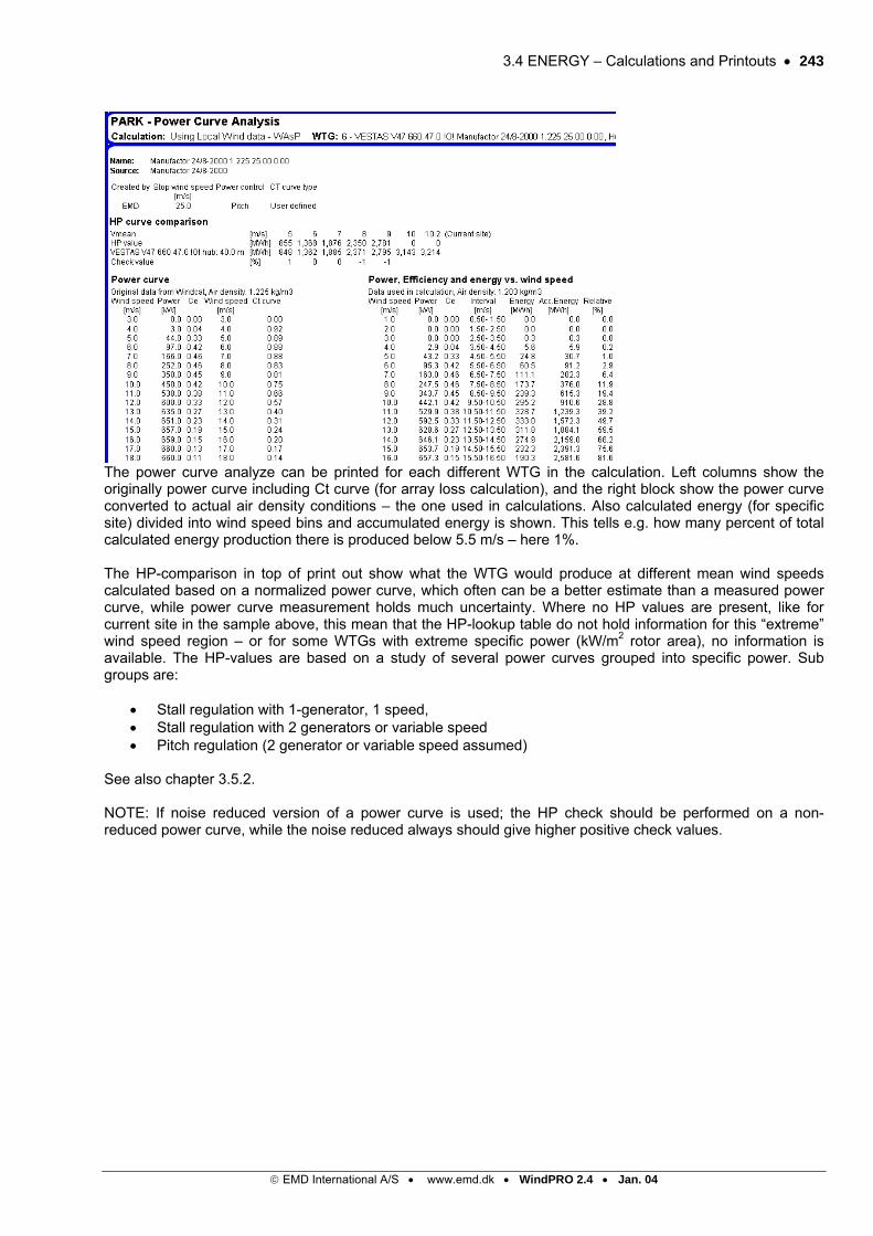
The power curve analyze can be printed for each different WTG in the calculation. Left columns show the originally power curve including Ct curve (for array loss calculation), and the right block show the power curve converted to actual air density conditions – the one used in calculations. Also calculated energy (for specific site) divided into wind speed bins and accumulated energy is shown. This tells e.g. how many percent of total calculated energy production there is produced below 5.5 m/s – here 1%. The HP-comparison in top of print out show what the WTG would produce at different mean wind speeds calculated based on a normalized power curve, which often can be a better estimate than a measured power curve, while power curve measurement holds much uncertainty. Where no HP values are present, like for current site in the sample above, this mean that the HP-lookup table do not hold information for this “extreme” wind speed region – or for some WTGs with extreme specific power (kW/m2 rotor area), no information is available. The HP-values are based on a study of several power curves grouped into specific power. Sub groups are:

• Stall regulation with 1-generator, 1 speed, • Stall regulation with 2 generators or variable speed • Pitch regulation (2 generator or variable speed assumed)

See also chapter 3.5.2. NOTE: If noise reduced version of a power curve is used; the HP check should be performed on a non-reduced power curve, while the noise reduced always should give higher positive check values.




Wind data can in print be compared with a reference, which is fixed to “flat terrain, roughness class 1”. This reference is chosen while this is the “best onshore” condition and thereby the effects of coast near site, hilly site etc. will be seen clearly – in the above it is seen that the site benefits much from the local orography in most sectors, while they all offers much more energy than a flat roughness class 1 site.

As an alternative to comparing to reference, a more detailed color set-up can be made, where the roses for energy and frequency are divided into wind speed intervals.


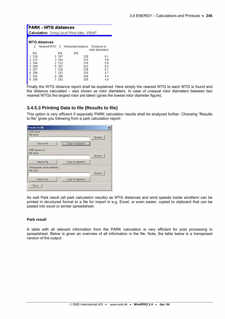
Finally the WTG distance report shall be explained. Here simply the nearest WTG to each WTG is found and the distance calculated – also shown as rotor diameters. In case of unequal rotor diameters between two nearest WTGs the largest rotor are taken (gives the lowest rotor diameter figure).

3.4.5.3 Printing Data to file (Results to file) This option is very efficient if especially PARK calculation results shall be analyzed further. Choosing “Results to file” gives you following from a park calculation report:

As well Park result (all park calculation results) as WTG distances and wind speeds inside windfarm can be printed in structured format to a file for import in e.g. Excel, or even easier, copied to clipboard that can be pasted into excel or similar spreadsheet.

Park result A table with all relevant information from the PARK calculation is very efficient for post processing in spreadsheet. Below is given an overview of all information in the file. Note, the table below is a transposed version of the output.




Label Example Explanation

WTG num 1WTG numbered from 1 with lowest system label first

WTG type New New or existing

LIB file ES Munesia-40m1.lib WindstatisticEast 318.391 CoordinateNorth 4.540.176 CoordinateZ 581 h.a.s.lValid Yes Refer to power curveManufact. DUMMY Refer to power curveType Refer to power curvePower 3.500 Refer to power curveDiam. 100 Refer to power curveHeight 95 hub height

Row data/Description 126.6°, 200.0 mIf row of WTGs the angle and distance else description field

Creator USER Refer to power curve

NameConstructed based on 3MW expirience Refer to power curve

User label WTG#1 User label

Result 7.027,10Calc. result incl park efficiency, no uncertainty withdrawn

Efficiency 97,1 Park efficiencyRegional Correction Factor 1 Refer to wind statistic

Equivalent roughness 2,1

is the roughness class in flat terrain with no obstacles that would give the same calculated energy production

Mean wind speed 6,3 Calculated at hub height

HP result (std. air density) 7.023,00Calculation result based on HP table lookup instead of "real" power curve

Calculated prod. without new WTGs 0 Calculation of existing WTG without new

Actual wind corrected energy 0Actual production from "statistics" of existing WTG

Goodness Factor Actual/calc. for exisitng WTGA (Sum) 7 Weibull A-parameter, all sectorsk (Sum) 1,72 Weibull k-parameter, all sectorsA (0) 9,1 Weibull A-parameter, sector 0 (North)k (0) 1,93 Weibull k-parameter, sector 0 (Northf (0) 9,3 Frequency, sector 0 (North)A (1) 5 As above, sector 1

k (1) 1,92 As above, sector 1

f (1) 5,8 As above, sector 1

For all following sectors the same as abowe

Wind speeds inside windfarm First it can be defined for which wind speeds and which angles and for which sites, the data shall be extracted.

Specification of where and in which resolution the data is needed. Explanation: Wind speeds - first row the "unreduced" (center value for interval), below in table the reduced

UTM ED50 Zone: 32 East: 603066 North: 6225290 1300ÅQ: 1.300 kW NORDEX - Skovgårde EbeltoDirections: 1,5 2,5 3,5 4,5 5,5 6,5 7,5 8,5 9,5 10,5(center of 0,5 1,5 2,5 3,5 4,5 5,5 6,5 7,5 8,5 9,5 10,5direction 30,5 1,5 2,5 3,5 4,5 5,5 6,5 7,5 8,5 9,5 10,5interval) 60,5 1,5 2,5 3,5 4,5 5,5 6,5 7,5 8,5 9,5 10,5

90,5 1,5 2,5 3,5 4,5 5,5 6,5 7,5 8,5 9,5 10,5120,5 1,5 2,5 3,5 4,5 5,5 6,5 7,5 8,5 9,5 10,5150,5 1,49 2,49 3,42 4,24 5,17 6,1 7,07 8,04 9,03 10,04180,5 1,46 2,44 3,26 3,77 4,33 5,08 5,81 6,64 7,54 8,48210,5 1,5 2,5 3,5 4,5 5,5 6,5 7,5 8,5 9,5 10,5240,5 1,5 2,5 3,5 4,5 5,5 6,5 7,5 8,5 9,5 10,5270,5 1,5 2,5 3,5 4,5 5,5 6,5 7,5 8,5 9,5 10,5300,5 1,5 2,5 3,5 4,5 5,5 6,5 7,5 8,5 9,5 10,5330,5 1,5 2,5 3,5 4,5 5,5 6,5 7,5 8,5 9,5 10,5

The table holds the needed information, which e.g. can be used for cleaning measurements in a windfarm. But this need some “reverse engineering” to do this. The Lookup function in excels is important for this purpose.

3.5 ENERGY - Uncertainty and Control • 247


3.5 ENERGY - Uncertainty and Control

3.5.0 Introduction to Uncertainty and Control To carry out a production calculation by using a modern computer program is worthwhile the work. However, as large-scaled investments are usually involved in wind energy projects, it is important that the user of the program also is able to control whether the results are realistic or not. The many detailed printouts from WindPRO are of good help - further possibilities will be described in the following.

3.5.1 Uncertainties The following uncertainties are usually present in a production calculation (figures in brackets indicate estimated uncertainties under good conditions):

• The Wind Statistics (5%) • The Terrain Description, i.e. roughness, hills and obstacles (5%) • The Power Curve (5% if controlled, see section 5.2) • The calculation method (5% for normal, not too complex terrain)

A commonly used way of estimating the joint uncertainty of independent (un-correlated) uncertainties is to calculate the RMS value, i.e.:

Joint uncertainty = SQRT(52+52+52+52)= SQRT(100) = 10% Furthermore, there is an uncertainty in establishing the production corrected to a “normal year”, i.e. the long term scaling of actual production figures. The following uncertainties are based on experience from WTGs in Denmark:

With one year of production data +/- 10% With two years of production data +/- 5%

It is generally assumed that a good production estimate can be made with an uncertainty of +/-10% (Danish or similar conditions). This seems to be the case for about 95% of all calculations carried out in Denmark over the last years. Especially two things are very important in order to reach a low uncertainty:

• Experience with installations in the area which have been running for some years • Experience in using the method and regular control of your own calculations.

One would therefore expect that 95% of the production estimates, which have been made by an experienced user/consultant in Denmark and Germany, lie within +/-10%. For new regions where there is no experience, a significant increase in the uncertainty should be expected, especially in complex terrain. It is not possible to set any guidelines for these uncertainties. One thing is uncertainty another is error. If data are erroneous, there is no upper limit for how incorrect the estimated production can be compared to the actual production.

3.5.2 Checking the Power Curve A key parameter when controlling the power curve is the non-dimensional Ce curve, which can be used for direct comparison of different power curves. If the maximum Ce value exceeds 0.45, either the power curve is incorrect or the manufacturer has developed an extremely efficient WTG.

248 • 3.5 ENERGY - Uncertainty and Control


Comparison of Ce curves from WTGs of similar construction and size is also a good way to look for errors. The figure above shows a power curve measurement that should have been rejected in the first place due to a unrealistic high Ce value.

Another possible method of verification is to compare the estimated production by using the “Helge Petersen” (HP) curves with the production based on the power curve. The HP curves are shown in the above figure. These curves show key figures based on a large number of rather new turbines ranging from 150 kW to 2 MW. These curves have been updated in 2001, and a printout from the WTG Catalog will give the values from these curves for the specific WTG. Comparisons with actual power curve calculations are performed; see part of print from WTG catalogue below.



New from version 2.4: From version 2.4 the HP values has been improves with following: WTGs smaller than 150 kW are given reduced HP values based on experience, so that: 50-149 kW is reduced to 90% for 50 kW linear reduced up 100% at 150 kW. WTGs below 50 kW are reduced to 90%. 1 generator pitch regulated WTGs are reduced with 4% for mean wind speeds below 7 m/s. With these corrections, the HP values will be more well working for all WTG sizes.

3.5.3 Verification by using existing WTGs The best check is, however, to use production information for other WTGs in the area for which reliable information is available. Information on the energy production and the power curve is essential. Regarding the production, it is important to adjust data from short measuring periods (less than 3 years) to long-term wind conditions (normal year). For Denmark, Holland and Germany there are good wind energy indices available. Do, however, notice the comments at the end of this section regarding possible errors when making a production verification. In other countries where no energy indices are available, but where several WTGs have been installed, you can establish your own index based on the WTGs with more than 3 years of operation. Performing a production calculation for the existing WTGs while using the same assumptions and data as used for the new WTGs - if necessary, adjusted to the existing terrain conditions if the terrain of the ‘old’ sites varies from the terrain conditions of new site carries out the production control. If the calculated production differs with more than about 5% you should be able to find the explanation. Possible reasons for errors in the production control for shorter production periods (less than 3 years):

1. The wind direction The production of a WTG sited in a terrain with very different roughness in the different direction sectors will be very sensitive to the prevailing wind directions during the reference period.

2. Seasonal variations A WTG sited in an area with many crossing hedges and/or large roughness will produce much less of its annual production during the summer with relatively weak wind than a coastal or offshore WTG, which relatively does not benefit as much from the strong winter storms as the low wind sited WTG - even when both WTGs would be running at their maximum output.

3. Geographic differences Even over distances of a few hundred kilometers in simple terrain there can easily be significant differences in the geostrophic winds.

4. The Power Curve Especially the ratio between swept rotor area and the nominal generator rating, but also the power regulation system (stall/pitch regulation) influences the production control. During a period with high winds, some WTGs with pronounced stall characteristics will only produce say 2/3 of their rated power, while other WTGs may produce even 1/3 above their rated power. Finally, some WTGs will have lower stop wind speeds than other.

3.5.4 Verification by using additional wind data If no “reference turbines” is available in the area, then verification calculations on the basis of other wind data will give a good indication of the level of uncertainty by a simple comparison of results. One should generally never base production estimation on only one set of wind measurements unless these have been verified through other measurements. The risk of not noticing errors is simply too high. EMD has made a more comprehensive study regarding checking existing wind farms energy production against calculations, where many different investigations have been performed. The complete study can be downloaded from EMD’s home page: www.emd.dk. Below main result graphic is shown.

http://www.emd.dk/

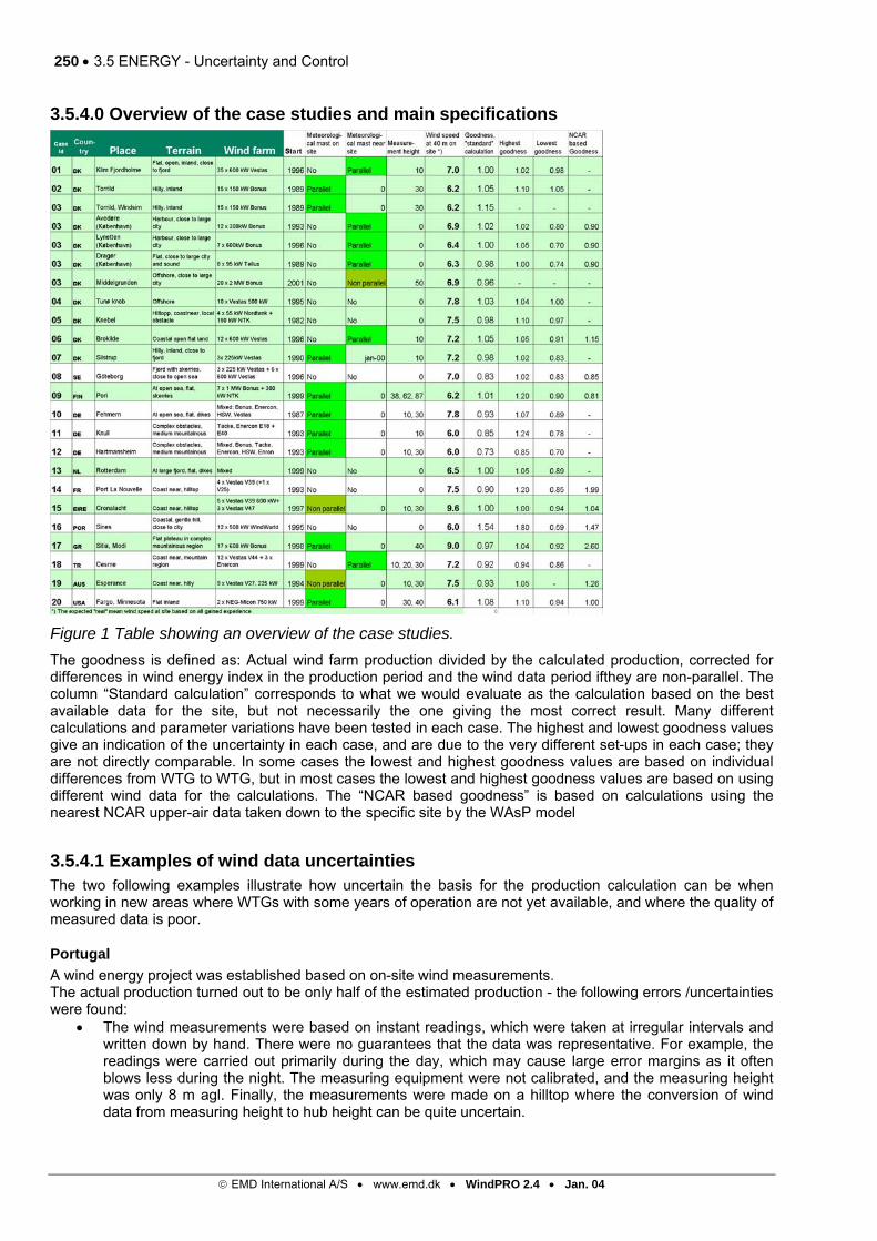
250 • 3.5 ENERGY - Uncertainty and Control


3.5.4.0 Overview of the case studies and main specifications

Figure 1 Table showing an overview of the case studies. The goodness is defined as: Actual wind farm production divided by the calculated production, corrected for differences in wind energy index in the production period and the wind data period ifthey are non-parallel. The column “Standard calculation” corresponds to what we would evaluate as the calculation based on the best available data for the site, but not necessarily the one giving the most correct result. Many different calculations and parameter variations have been tested in each case. The highest and lowest goodness values give an indication of the uncertainty in each case, and are due to the very different set-ups in each case; they are not directly comparable. In some cases the lowest and highest goodness values are based on individual differences from WTG to WTG, but in most cases the lowest and highest goodness values are based on using different wind data for the calculations. The “NCAR based goodness” is based on calculations using the nearest NCAR upper-air data taken down to the specific site by the WAsP model

3.5.4.1 Examples of wind data uncertainties The two following examples illustrate how uncertain the basis for the production calculation can be when working in new areas where WTGs with some years of operation are not yet available, and where the quality of measured data is poor.

Portugal A wind energy project was established based on on-site wind measurements. The actual production turned out to be only half of the estimated production - the following errors /uncertainties were found:

• The wind measurements were based on instant readings, which were taken at irregular intervals and written down by hand. There were no guarantees that the data was representative. For example, the readings were carried out primarily during the day, which may cause large error margins as it often blows less during the night. The measuring equipment were not calibrated, and the measuring height was only 8 m agl. Finally, the measurements were made on a hilltop where the conversion of wind data from measuring height to hub height can be quite uncertain.


• The use of the wind statistics from the nearest meteorological station would have given much more precise results. However, this station was rejected in the first place due to its complex location close to the ocean and the city.

Ireland In connection with a project, on-site measured data were received from the client. Data from the European Wind Atlas were available from 3 stations - all within about 70 km from the site. The calculations based on the data from the European Wind Atlas and the on-site measurements respectively gave the following results: Data origin Relative calculated

production Station 1 100% Station 2 92% Station 3 56% On-site measurements 163%

It can be seen that the deviations are large - a factor 3 from lowest to highest production. This clearly indicates that one should never rely on only one set of data unless these are very well documented.

3.5.4.2 Verification by using more wind atlas for a large area If a large number of wind atlas (wind statistics) are available for a large area (e.g. a country or a province), you can verify these by calculating the energy production on the basis of the same WTG and the same assumptions (e.g. Roughness Class 1 in all directions), and calculate the associated production indices (using the average of all the production figures). The resulting indices (e.g. in percent) are marked at the corresponding geographic positions on a map. You can then try to fit smooth curves through points of equal or close to equal indices. In general, the geotropic wind (which the Wind Atlases should represent) will only change a little over a certain area. It should therefore be possible to fit smooth curves without sharp bends. This exercise will often reveal incorrect Wind Atlas. The next figure shows a control of some Swedish Wind Atlas. As supporting data for the curve fitting around Denmark, the actual production from a number of turbines was also used.


3. windpro energy - institut for...

Documents