3-dimensional weakly admissible meshes: interpolation …demarchi/slides/slideshagen2011.pdf ·...

3-dimensional Weakly Admissible Meshes:interpolation and cubature ∗

Stefano De Marchi

Department of Pure and Applied MathematicsUniversity of Padova

Hagen, September 27, 2011

∗Joint work with M. Vianello (Padova, I)

Stefano De Marchi (DMPA-UNIPD) 3dimensional WAM Hagen, September 27, 2011 1 / 38

Outline

1 Motivations

2 Fekete points

3 (Weakly) Admissible Meshes, (W)AM

4 Approximate Fekete Points and Discrete Leja Points

5 1-dimensional WAMs

6 2-dimensional WAMs

7 3-dimensional WAMsCones (truncated)Toroidal sections

8 Interpolation, LS & cubature

9 Numerical examples


Motivations

Motivations and aims

Computation of near optimal points, for polynomial interpolation in themultivariate setting, such as Fekete points, ...

(Weakly) Admissible meshes, (W)AM: play a central role in the constructionof multivariate polynomial approximation processes on compact sets.

Theory vs computation: 2-dimensional and (simple) 3-dimensional (W)AMsare easy to construct. What’s about more general domains such as(truncated) cones or rotational sets like toroidal domains?


Fekete points

Notation

K ⊂ Rd (or Cd) compact set or manifold

p = {pj}1≤j≤N , N = dim(Pdn(K )) polynomial basis

ξ = {ξ1, . . . , ξN} ⊂ K interpolation points

V (ξ,p) = [pj(ξi )] Vandermonde matrix, det(V ) 6= 0

Πnf (x) =∑N

j=1 f (ξj) `j(x), interpolating polynomial with `j indeterminantal Lagrange formula

`j(x) =det(V (ξ1, . . . , ξj−1, x , ξj+1, . . . , ξN))

det(V (ξ1, . . . , ξj−1, ξj , ξj+1, . . . , ξN)), `j(ξi ) = δij


Fekete points

Fekete points: definition and properties

1 Fekete points: |det(V (ξ1, . . . , ξN))| is max in KN .

2 Lebesgue constant Λn = maxx∈K

N∑j=1

|`j(x)| ≤ N

3 Fekete points (and Lebesgue constants) are independent of the choiceof the basis

4 Fekete points are analytically known only in a few cases.interval: Gauss-Lobatto points, Λn = O(log n)complex circle: equispaced points, Λn = O(log n)cube: for tensor-product polynomials, Λn = O(logd n)

5 recent important result: Fekete points are asymptoticallyequidistributed w.r.t. the pluripotential equilibrium measure of K[Berman/Boucksom/Nystrom 2011]

6 open problem: efficient computation, even in the univariate complexcase (large scale optimization problem in N × d variables[Bos/Sommariva/Vianello 2011])


Fekete points

Idea

Extract Fekete points from a discretization of K

Which could be a suitable discretizaion of K?


(Weakly) Admissible Meshes, (W)AM

(Weakly) Admissible Meshes , (W)AM

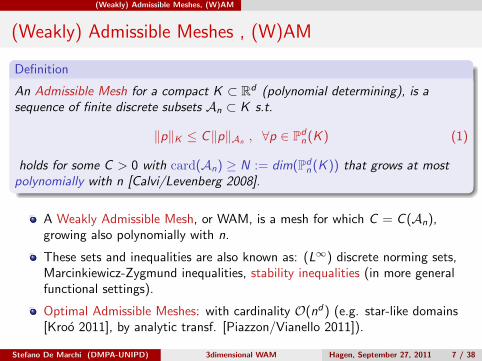
Definition

An Admissible Mesh for a compact K ⊂ Rd (polynomial determining), is asequence of finite discrete subsets An ⊂ K s.t.

‖p‖K ≤ C‖p‖An , ∀p ∈ Pdn(K ) (1)

holds for some C > 0 with card(An) ≥ N := dim(Pdn(K )) that grows at most

polynomially with n [Calvi/Levenberg 2008].

A Weakly Admissible Mesh, or WAM, is a mesh for which C = C (An),growing also polynomially with n.

These sets and inequalities are also known as: (L∞) discrete norming sets,Marcinkiewicz-Zygmund inequalities, stability inequalities (in more generalfunctional settings).

Optimal Admissible Meshes: with cardinality O(nd) (e.g. star-like domains[Kroo 2011], by analytic transf. [Piazzon/Vianello 2011]).



Weakly Admissible Meshes: properties

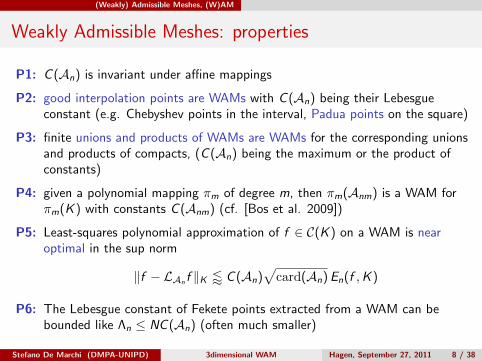
P1: C (An) is invariant under affine mappings

P2: good interpolation points are WAMs with C (An) being their Lebesgueconstant (e.g. Chebyshev points in the interval, Padua points on the square)

P3: finite unions and products of WAMs are WAMs for the corresponding unionsand products of compacts, (C (An) being the maximum or the product ofconstants)

P4: given a polynomial mapping πm of degree m, then πm(Anm) is a WAM forπm(K ) with constants C (Anm) (cf. [Bos et al. 2009])

P5: Least-squares polynomial approximation of f ∈ C(K ) on a WAM is nearoptimal in the sup norm

‖f − LAn f ‖K / C (An)√

card(An) En(f ,K )

P6: The Lebesgue constant of Fekete points extracted from a WAM can bebounded like Λn ≤ NC (An) (often much smaller)



Discrete Extremal Sets

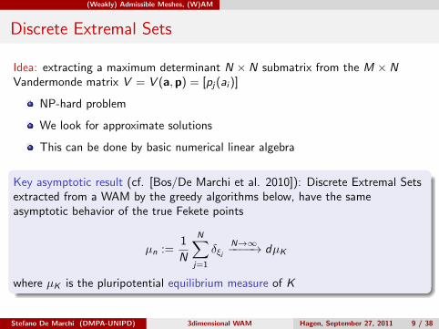
Idea: extracting a maximum determinant N × N submatrix from the M × NVandermonde matrix V = V (a,p) = [pj(ai )]

NP-hard problem

We look for approximate solutions

This can be done by basic numerical linear algebra

Key asymptotic result (cf. [Bos/De Marchi et al. 2010]): Discrete Extremal Setsextracted from a WAM by the greedy algorithms below, have the sameasymptotic behavior of the true Fekete points

µn :=1

N

N∑j=1

δξjN→∞−−−−→ dµK

where µK is the pluripotential equilibrium measure of K


Approximate Fekete Points and Discrete Leja Points

Approximate Fekete Points: algorithm

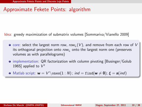
Idea: greedy maximization of submatrix volumes [Sommariva/Vianello 2009]

core: select the largest norm row, rowik (V ), and remove from each row of Vits orthogonal projection onto rowik onto the largest norm one (preservesvolumes as with parallelograms)

implementation: QR factorization with column pivoting [Businger/Golub1965] applied to V t

Matlab script: w = V ′\ones(1 : N) ; ind = find(w 6= 0); ξ = a(ind)


Approximate Fekete Points and Discrete Leja Points

Discrete Leja Points: algorithm

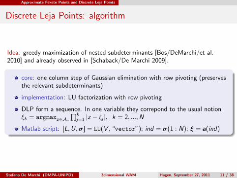
Idea: greedy maximization of nested subdeterminants [Bos/DeMarchi/et al.2010] and already observed in [Schaback/De Marchi 2009].

core: one column step of Gaussian elimination with row pivoting (preservesthe relevant subdeterminants)

implementation: LU factorization with row pivoting

DLP form a sequence. In one variable they correpond to the usual notionξk = argmaxz∈An

∏kj=1 |z − ξj |, k = 2, ...,N

Matlab script: [L,U,σ] = LU(V , “vector”); ind = σ(1 : N); ξ = a(ind)


1-dimensional WAMs

AFP in one variable

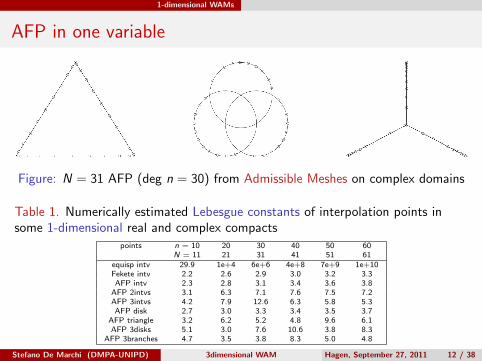
Figure: N = 31 AFP (deg n = 30) from Admissible Meshes on complex domains

Table 1. Numerically estimated Lebesgue constants of interpolation points insome 1-dimensional real and complex compacts

points n = 10 20 30 40 50 60N = 11 21 31 41 51 61

equisp intv 29.9 1e+4 6e+6 4e+8 7e+9 1e+10Fekete intv 2.2 2.6 2.9 3.0 3.2 3.3AFP intv 2.3 2.8 3.1 3.4 3.6 3.8

AFP 2intvs 3.1 6.3 7.1 7.6 7.5 7.2AFP 3intvs 4.2 7.9 12.6 6.3 5.8 5.3AFP disk 2.7 3.0 3.3 3.4 3.5 3.7

AFP triangle 3.2 6.2 5.2 4.8 9.6 6.1AFP 3disks 5.1 3.0 7.6 10.6 3.8 8.3

AFP 3branches 4.7 3.5 3.8 8.3 5.0 4.8


2-dimensional WAMs

2-dimensional WAMS: disk, triangle, square

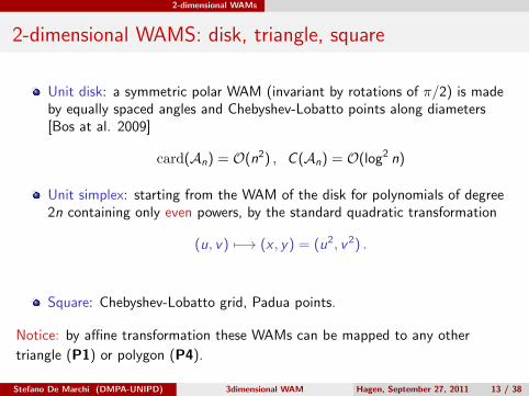
Unit disk: a symmetric polar WAM (invariant by rotations of π/2) is madeby equally spaced angles and Chebyshev-Lobatto points along diameters[Bos at al. 2009]

card(An) = O(n2) , C (An) = O(log2 n)

Unit simplex: starting from the WAM of the disk for polynomials of degree2n containing only even powers, by the standard quadratic transformation

(u, v) 7−→ (x , y) = (u2, v 2) .

Square: Chebyshev-Lobatto grid, Padua points.

Notice: by affine transformation these WAMs can be mapped to any other

triangle (P1) or polygon (P4).


2-dimensional WAMs

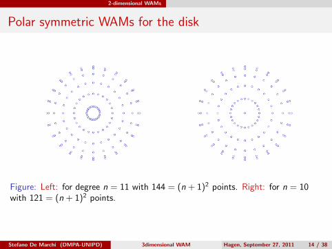
Polar symmetric WAMs for the disk

Figure: Left: for degree n = 11 with 144 = (n + 1)2 points. Right: for n = 10with 121 = (n + 1)2 points.


2-dimensional WAMs

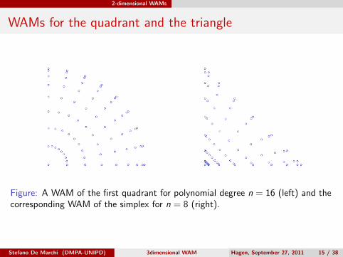
WAMs for the quadrant and the triangle

Figure: A WAM of the first quadrant for polynomial degree n = 16 (left) and thecorresponding WAM of the simplex for n = 8 (right).


2-dimensional WAMs

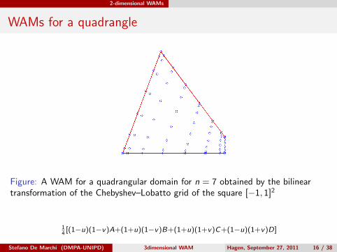
WAMs for a quadrangle

Figure: A WAM for a quadrangular domain for n = 7 obtained by the bilineartransformation of the Chebyshev–Lobatto grid of the square [−1, 1]2

14

[(1−u)(1−v)A+(1+u)(1−v)B+(1+u)(1+v)C+(1−u)(1+v)D]


2-dimensional WAMs

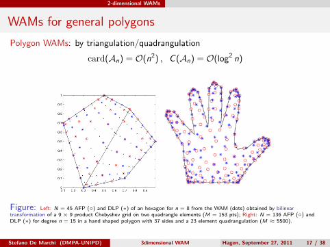
WAMs for general polygons

Polygon WAMs: by triangulation/quadrangulation

card(An) = O(n2) , C (An) = O(log2 n)

Figure: Left: N = 45 AFP (◦) and DLP (∗) of an hexagon for n = 8 from the WAM (dots) obtained by bilineartransformation of a 9 × 9 product Chebyshev grid on two quadrangle elements (M = 153 pts); Right: N = 136 AFP (◦) andDLP (∗) for degree n = 15 in a hand shaped polygon with 37 sides and a 23 element quadrangulation (M ≈ 5500).


2-dimensional WAMs

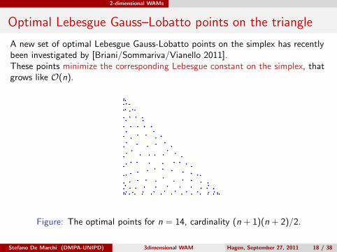
Optimal Lebesgue Gauss–Lobatto points on the triangle

A new set of optimal Lebesgue Gauss-Lobatto points on the simplex has recentlybeen investigated by [Briani/Sommariva/Vianello 2011].These points minimize the corresponding Lebesgue constant on the simplex, thatgrows like O(n).

Figure: The optimal points for n = 14, cardinality (n + 1)(n + 2)/2.


3-dimensional WAMs Cones (truncated)

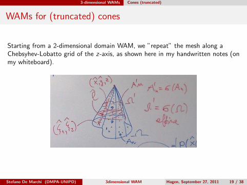
WAMs for (truncated) cones

Starting from a 2-dimensional domain WAM, we ”repeat” the mesh along aChebsyhev-Lobatto grid of the z-axis, as shown here in my handwritten notes (onmy whiteboard).



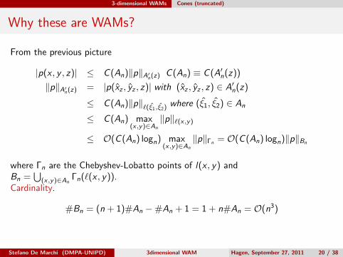
Why these are WAMs?

From the previous picture

|p(x , y , z)| ≤ C (An)‖p‖A′n(z) C (An) ≡ C (A′n(z))

‖p‖A′n(z) = |p(xz , yz , z)| with (xz , yz , z) ∈ A′n(z)

≤ C (An)‖p‖`(ξ1,ξ2) where (ξ1, ξ2) ∈ An

≤ C (An) max(x,y)∈An

‖p‖`(x,y)

≤ O(C (An) logn) max(x,y)∈An

‖p‖Γn = O(C (An) logn)‖p‖Bn

where Γn are the Chebyshev-Lobatto points of l(x , y) andBn =

⋃(x,y)∈An

Γn(`(x , y)).Cardinality.

#Bn = (n + 1)#An −#An + 1 = 1 + n#An = O(n3)



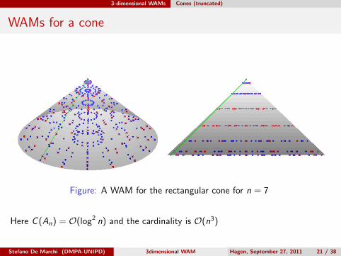
WAMs for a cone

Figure: A WAM for the rectangular cone for n = 7

Here C (An) = O(log2 n) and the cardinality is O(n3)



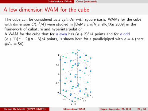
A low dimension WAM for the cube

The cube can be considered as a cylinder with square basis. WAMs for the cubewith dimension O(n3/4) were studied in [DeMarchi/Vianello/Xu 2009] in theframework of cubature and hyperinterpolation.A WAM for the cube that for n even has (n + 2)3/4 points and for n odd(n + 1)(n + 2)(n + 3)/4 points, is shown here for a parallelpiped with n = 4 (here#An = 54)



WAMs for a pyramid

Figure: A WAM for a non-rectangular pyramid and a truncated one, made byusing Padua points for n = 10. Notice the generating curve of Padua points thatbecomes a spiral

In this case C (An) = O(log2 n) and the cardinality is O(n3/2)


3-dimensional WAMs Toroidal sections

3-dimensional WAMs: toroidal sections

Starting from a 2-dimensional WAM, An, by rotation around a vertical axissampled at the 2n + 1 Chebyshev-Lobatto points of the arc of circumference, weget WAMs for the torus, sections of the torus and in general toroids.The resulting cardinality will be (2n + 1)×#An



Why these are WAMs?

From the previous ”picture” Given a polynomial p(x , y , z) ∈ P3n we can write it in

cylindrical coordinates getting

p(x , y , z) = q(r , z , φ) = s(x ′, y ′, φ) ∈ P2,(x′,y ′)n ⊗ Tφn

since

x iy jxk = (r cosφ)i (r sinφ)jzk(r0 + x ′)i cosi φ(r0 + y ′)j sinj φ(r0 + y ′)k



WAMs for toroidal sections: points on the disk

Figure: WAM for n = 5 on the torus centered in z0 = 0 of radius r0 = 3, with−2/3π ≤ θ ≤ 2/3π.

In this case C (An) = O(log2 n) and the cardinality is O(2n3)Stefano De Marchi (DMPA-UNIPD) 3dimensional WAM Hagen, September 27, 2011 26 / 38


WAMs for toroidal sections: Padua points

Figure: Padua points on the toroidal section with z0 = 0, r0 = 3 and opening−2/3π ≤ θ ≤ 2/3π.

In this case C (An) = O(log2 n) and the cardinality is O(n3).


Interpolation, LS & cubature

Interpolation and Least-Squares

1 Positive aspects:

1 AFP (and DLP) are near optimal interpolation points. We know themalso on subarc-based product WAMs on sections of disk,sphere,ball,torus, such as circular sectors and lenses, spherical caps, quandrangles,lunes, slices,.... with card(An) = O(nd) and C (An) = O(logk n),(k = 2 for surfaces, k = 3 for solids) [Bos/Vianello 2011,Bos/DeMarchi et al 2011]

2 so far, we can construct, by linear algebra approach, polynomialinterpolation and least-square approximation on AFP or DLP up todegree 30 on solid cones and torus.

2 Negative aspects.

1 Extracting AFP or DLP, is costly!2 Find good polynomial basis (for cylinders [Wade 2010, De

Marchi/Marchioro/Sommariva 2011]).


Interpolation, LS & cubature

Cubature

1 For (generalized) solid cones, in literature there exist cubature product ruleswith O(n3/8) points, e.g. [Stround 1971]. For the torus with circular andsquare cross-section the software STROUD (Matlab and C) by J. Burkardt2004-2009, implements Stroud formulas for cubature on the solid torus.

2 Our approach, uses as cubature points for torus with square, circular ortriangular cross-sections, the AFP/DLP. Cardinality O(n3/6) instead ofO(n3/2) (tensor product formulas of Burkardt). As polynomial basis we usetensor product Chebsyhev polynomials.


Numerical examples

Conic section: disk

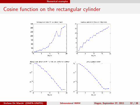
K is the solid cone. Given an n, then

The AFP are extracted from a WAM having O(n3) points

The polynomial basis is the tensor product Chebyshev polynomial basis.

The Lebesgue constant and the interpolation error has been computed on amesh of control points (consisting of the original WAM with 2n instead of n).

We also computed the

1 least-square operator norm, ‖LAn‖ = maxx∈K∑M

i=1 |gi (x)| wheregi , i = 1, . . . ,M are a set of generators and M ≥ N = dimP3

n (cf. [Bos/DeMarchi et al. 2010])

2 interpolation sup error ‖f − pn(f )‖∞3 least-square sup error ‖f − LAn(f )‖∞


Numerical examples

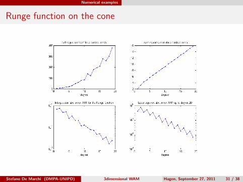
Runge function on the cone


Numerical examples

Cosine function on the rectangular cylinder


Numerical examples

Circular and square toric sections

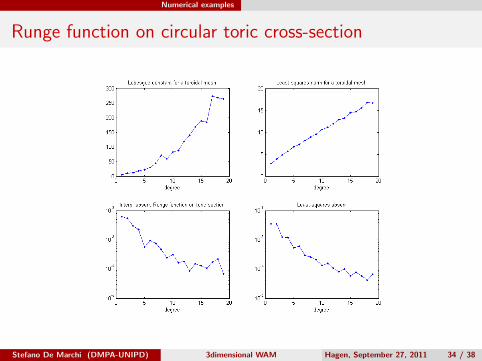
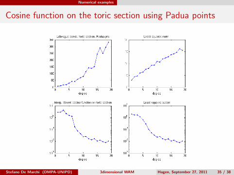
K is now a toric section. Given n then

The AFP are extracted from a WAM having (n + 1)2(2n + 1) points in the

case of the disk and (n+1)(n+2)2 (2n + 1) in the case of the square (by using

Padua points).

The polynomial basis is the tensor product Chebyshev polynomial basis.

The Lebesgue constant and the interpolation error has been computed on amesh of control points (the original WAM of degree 2n).

We computed as before least-square operator sup-norm, interpolation error

‖f − pn(f )‖∞ and least-square error ‖f − LAn(f )‖∞.


Numerical examples

Runge function on circular toric cross-section


Numerical examples

Cosine function on the toric section using Padua points


Numerical examples

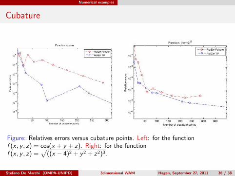
Cubature

Figure: Relatives errors versus cubature points. Left: for the functionf (x , y , z) = cos(x + y + z). Right: for the functionf (x , y , z) =

√((x − 4)2 + y 2 + z2)3.


Numerical examples

References

1 J.P. Calvi and N. Levenberg, Uniform approximation by discrete least squarespolynomials, J. Approx. Theory 152 (2008), 82–100.

2 L. Bos, S. De Marchi, A. Sommariva and M. Vianello, Computing multivariateFekete and Leja points by numerical linear algebra, SIAM J. Numer. Anal. 48(2010), 1984–1999.

3 F. Piazzon and M. Vianello, Analytic transformations of admissible meshes, East J.Approx. 16 (2010), 313–322.

4 A. Kroo, On optimal polynomial meshes, J. Approx. Theory (2011), to appear.

5 S. De Marchi, M. Marchiori and A. Sommariva, Polynomial approximation andcubature at approximate Fekete and Leja points of the cylinder, submitted 2011.

6 M. Briani, A. Sommariva and M. Vianello, Computing Fekete and Lebesguepoints: simplex, square, disk, submitted 2011.

7 L. Bos, S. De Marchi, A. Sommariva and M. Vianello, On Multivariate NewtonInterpolation at Discrete Leja Points , Accepted by Dolomites Res. Notes onApprox. (DRNA) (2011).

8 L. Bos and M. Vianello, Subperiodic trigonometric interpolation and quadrature,submitted (2011).


Numerical examples

Thank you for your attention

Dolomites Workshop on Constructive Approximation andApplications 2012, Alba di Canazei 7-12(?) September 2012


3-dimensional weakly admissible meshes: interpolation …demarchi/slides/slideshagen2011.pdf ·...

Documents