2.6 — Long Run Industry EquilibriumECON 306 · Microeconomic Analysis · Fall 2020Ryan SafnerAssistant Professor of Economics safner@hood.edu ryansafner/microF20microF20.classes.ryansafner.com

Firm's Long Run Supply Decisions

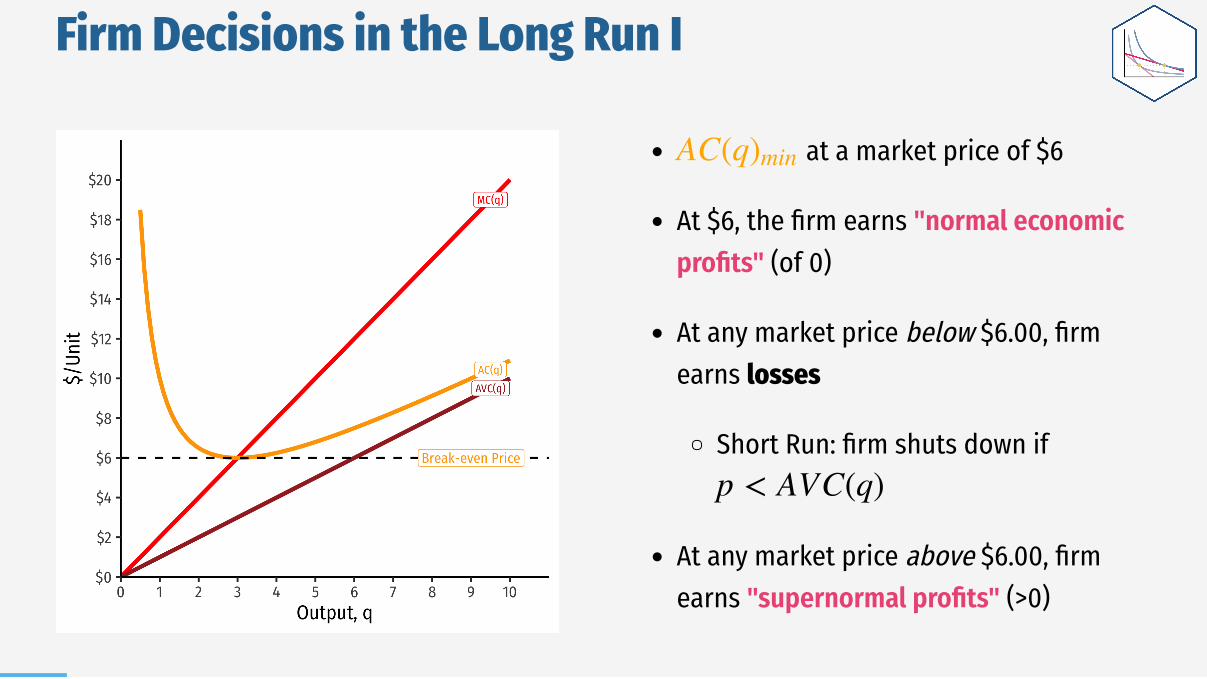
at a market price of $6

At $6, the firm earns "normal economicprofits" (of 0)

At any market price below $6.00, firmearns losses

Short Run: firm shuts down if

At any market price above $6.00, firmearns "supernormal profits" (>0)

Firm Decisions in the Long Run I

AC(q)min

p < AVC(q)

Short run: firms that shut down stuck in market, incur fixed

costs

Firm Supply Decisions in the Short Run vs. Long Run

( = 0)q∗

π = −f

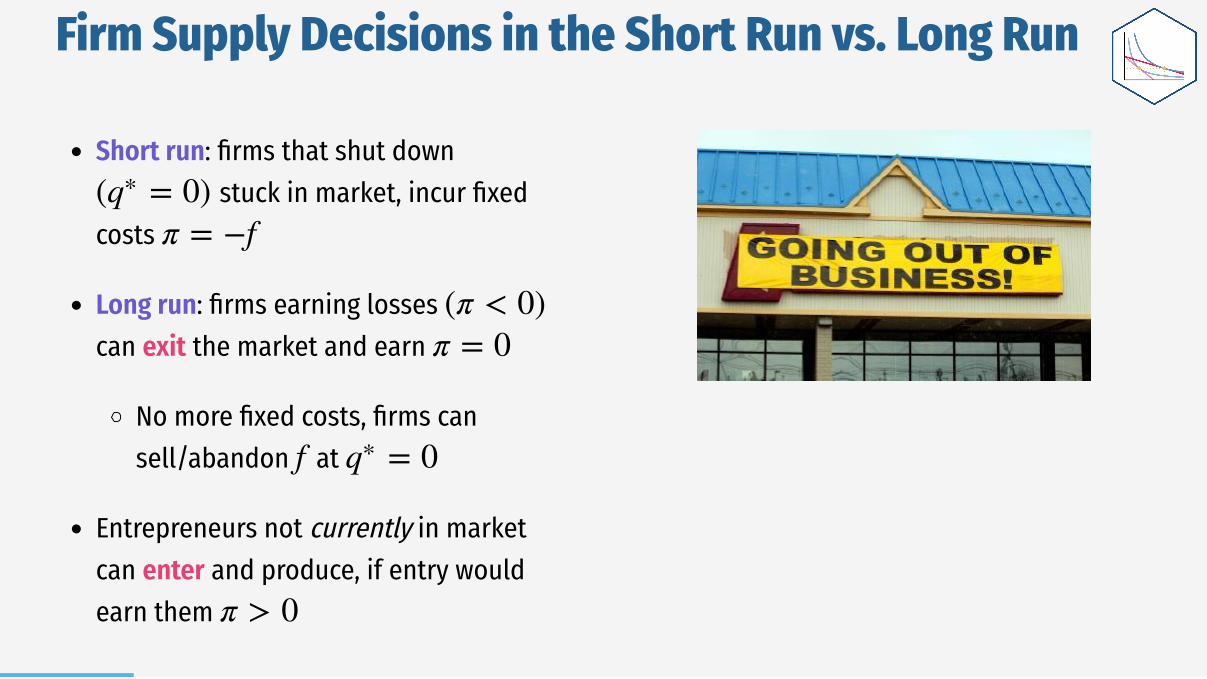
Short run: firms that shut down stuck in market, incur fixed

costs

Long run: firms earning losses can exit the market and earn

No more fixed costs, firms cansell/abandon at

Firm Supply Decisions in the Short Run vs. Long Run

( = 0)q∗

π = −f

(π < 0)

π = 0

f = 0q∗

Short run: firms that shut down stuck in market, incur fixed

costs

Long run: firms earning losses can exit the market and earn

No more fixed costs, firms cansell/abandon at

Entrepreneurs not currently in marketcan enter and produce, if entry wouldearn them

Firm Supply Decisions in the Short Run vs. Long Run

( = 0)q∗

π = −f

(π < 0)

π = 0

f = 0q∗

π > 0

Firm Supply Decisions in the Short Run vs. Long Run

When

Profits are negative

Short run: shut down production

Firm loses more by producing thanby not producing

Long run: firms in industry exit theindustry

No new firms will enter this industry

Firm's Long Run Supply: Visualizing

p < AVC

π

When

Profits are negative

Short run: continue production

Firm loses less by producing thanby not producing

Long run: firms in industry exit theindustry

No new firms will enter this industry

Firm's Long Run Supply: Visualizing

AVC < p < AC

π

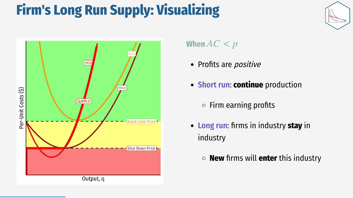
When

Profits are positive

Short run: continue production

Firm earning profits

Long run: firms in industry stay inindustry

New firms will enter this industry

Firm's Long Run Supply: Visualizing

AC < p

Production Rules, Updated:1. Choose such that

2. Profit

3. Shut down in short run if

4. Exit in long run if

q∗ MR(q) = MC(q)

π = q[p − AC(q)]

p < AVC(q)

p < AC(q)

Market Entry and Exit

Now we must combine optimizingindividual firms with market-wideadjustment to equilibrium

Since , in the longrun, profit-seeking firms will:

Exit, Entry, and Long Run Industry Equilibrium I

π = [p − AC(q)]q

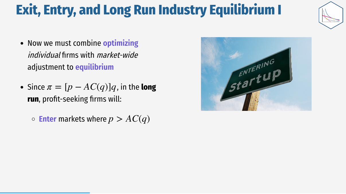
Now we must combine optimizingindividual firms with market-wideadjustment to equilibrium

Since , in the longrun, profit-seeking firms will:

Enter markets where

Exit, Entry, and Long Run Industry Equilibrium I

π = [p − AC(q)]q

p > AC(q)

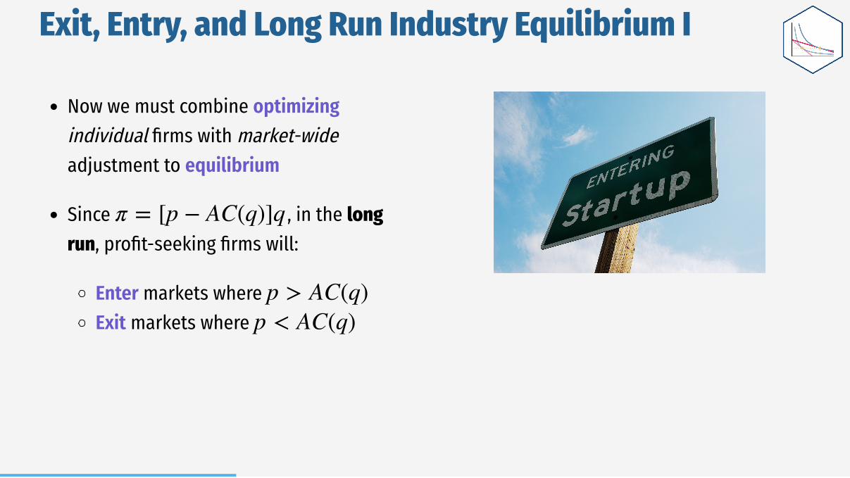
Now we must combine optimizingindividual firms with market-wideadjustment to equilibrium

Since , in the longrun, profit-seeking firms will:

Enter markets where Exit markets where

Exit, Entry, and Long Run Industry Equilibrium I

π = [p − AC(q)]q

p > AC(q)

p < AC(q)

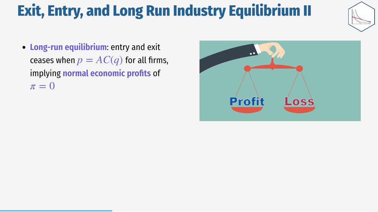
Long-run equilibrium: entry and exitceases when for all firms,implying normal economic profits of

Exit, Entry, and Long Run Industry Equilibrium II

p = AC(q)

π = 0

Long-run equilibrium: entry and exitceases when for all firms,implying normal economic profits of

Zero Economic Profits Theorem: long runeconomic profits for all firms in acompetitive industry are 0

Firms must earn an accounting profit tostay in business

Exit, Entry, and Long Run Industry Equilibrium II

p = AC(q)

π = 0

Deriving the Industry Supply Curve

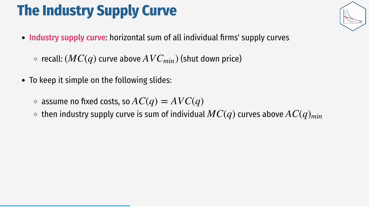
The Industry Supply CurveIndustry supply curve: horizontal sum of all individual firms' supply curves

recall: curve above (shut down price)

To keep it simple on the following slides:

assume no fixed costs, so then industry supply curve is sum of individual curves above

(MC(q) AV )Cmin

AC(q) = AVC(q)

MC(q) AC(q)min

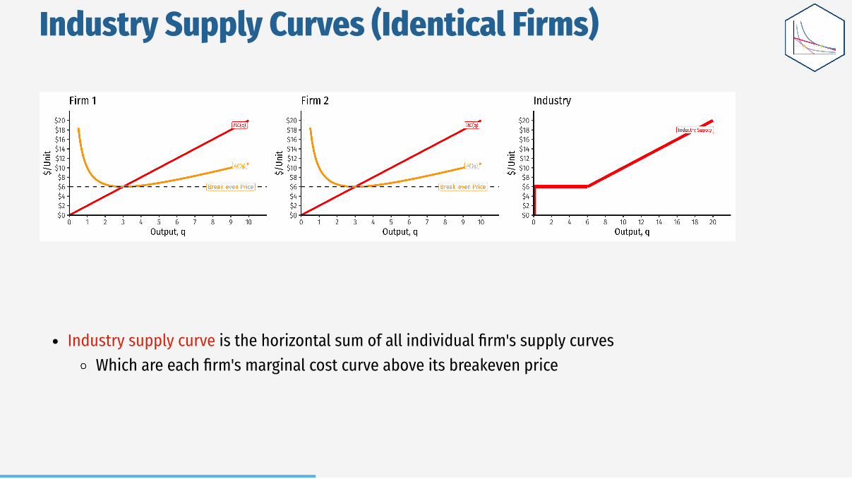
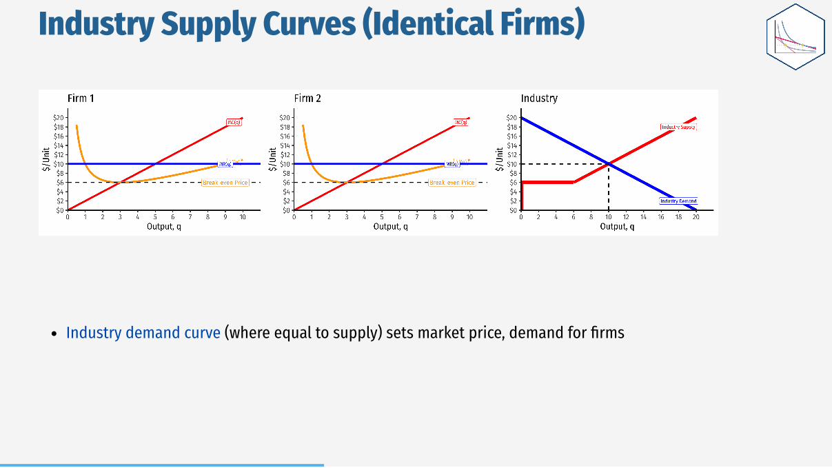
Industry Supply Curves (Identical Firms)

Industry supply curve is the horizontal sum of all individual firm's supply curvesWhich are each firm's marginal cost curve above its breakeven price

Industry Supply Curves (Identical Firms)

Industry demand curve (where equal to supply) sets market price, demand for firms

Industry Supply Curves (Identical Firms)

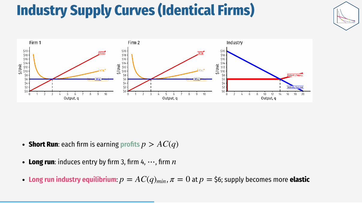
Short Run: each firm is earning profits

Long run: induces entry by firm 3, firm 4, , firm

Long run industry equilibrium:

p > AC(q)

⋯ n

Industry Supply Curves (Identical Firms)

Short Run: each firm is earning profits

Long run: induces entry by firm 3, firm 4, , firm

Long run industry equilibrium: , at $6; supply becomes more elastic

p > AC(q)

⋯ n

p = AC(q)min π = 0 p =

Zero Economic Profits & Economic Rents

Recall, we've essentially defined a firm asa completely replicable recipe(production function) of resources

"Any idiot" can enter market, buyrequired factors, and produce atmarket price and earn the market rateof

Back to Zero Economic Profits

q = f (L, K)

q∗

p

π

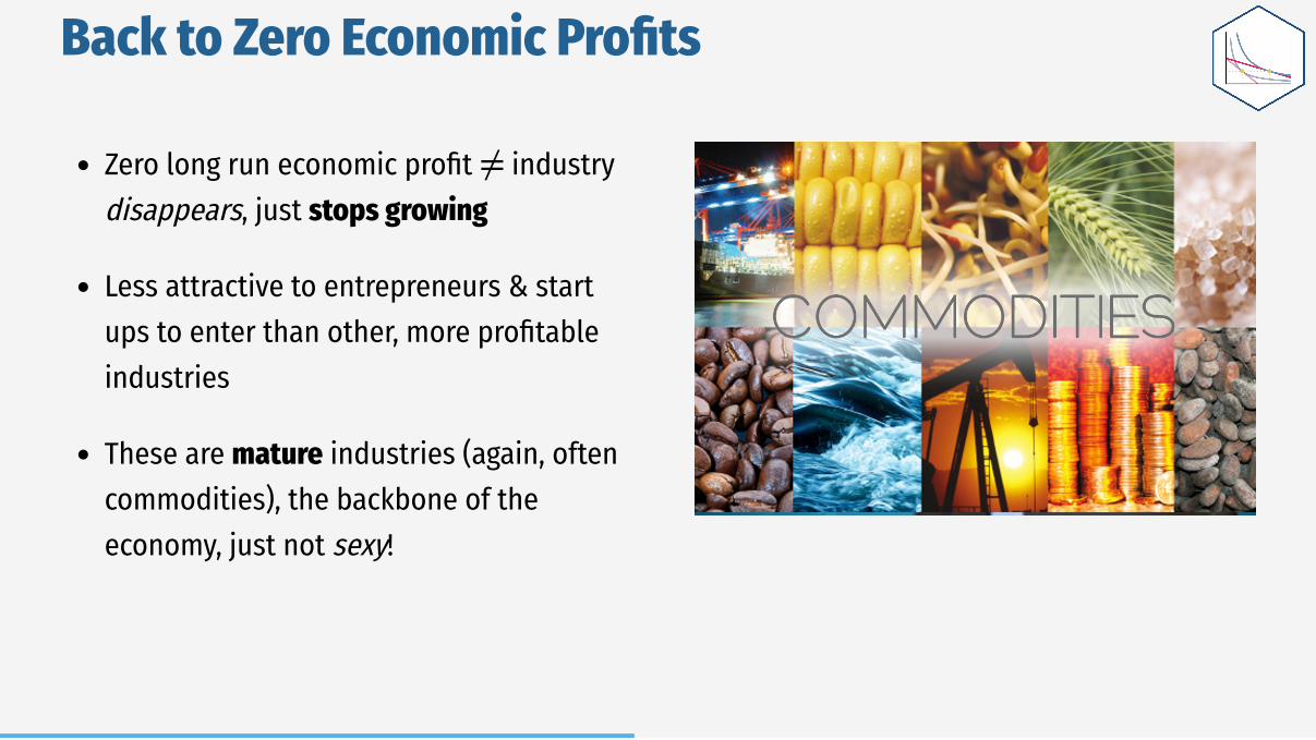
Zero long run economic profit industrydisappears, just stops growing

Less attractive to entrepreneurs & startups to enter than other, more profitableindustries

These are mature industries (again, oftencommodities), the backbone of theeconomy, just not sexy!

Back to Zero Economic Profits

≠

All factors being paid their market price

i.e. their opportunity cost - the samethat they could earn elsewhere ineconomy

Firms earning normal market rate ofreturn

No excess rewards (economic profits)to attract new resources into theindustry, nor losses to bleedresources out of industry

Back to Zero Economic Profits

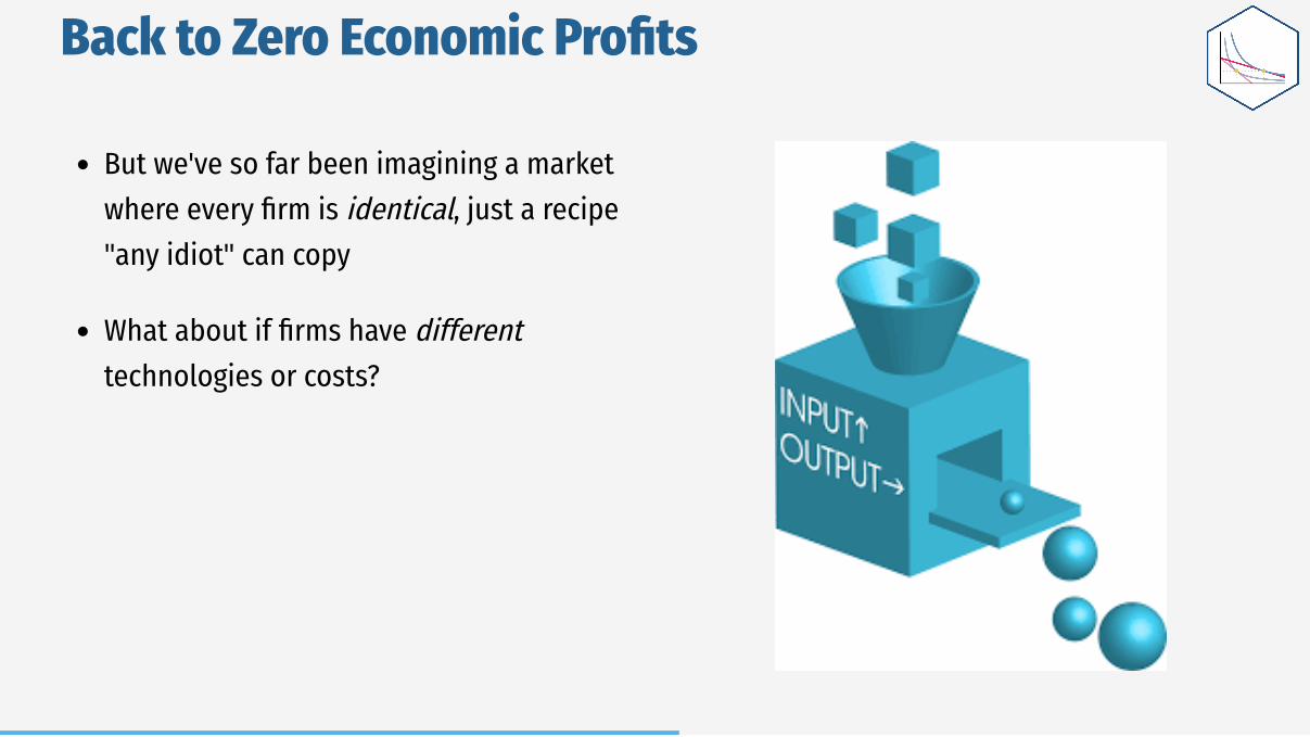
But we've so far been imagining a marketwhere every firm is identical, just a recipe"any idiot" can copy

What about if firms have differenttechnologies or costs?

Back to Zero Economic Profits

Firms have different technologies/costsdue to relative differences in:

Managerial talentWorker talentLocationFirst-mover advantageTechnological secrets/IPLicense/permit accessPolitical connectionsLobbying

Let's derive industry supply curve again,and see if this may affact profits

Industry Supply Curves (Different Firms) I

Industry Supply Curves (Different Firms) II

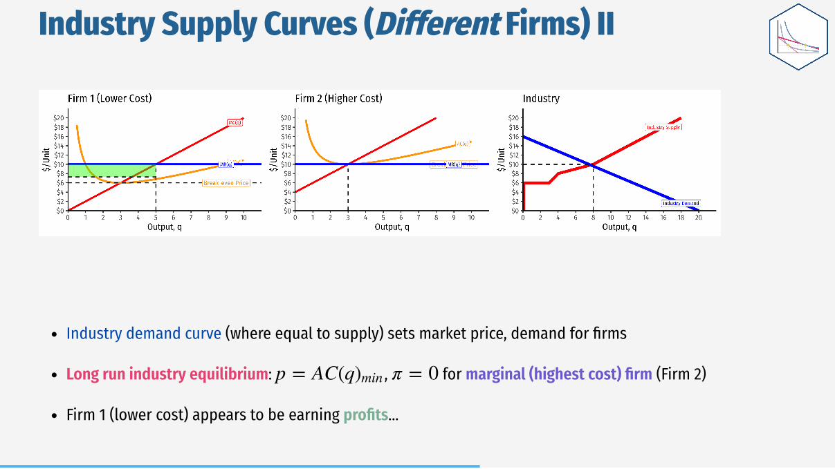
Industry supply curve is the horizontal sum of all individual firm's supply curvesWhich are each firm's marginal cost curve above its breakeven price

Industry Supply Curves (Different Firms) II

Industry demand curve (where equal to supply) sets market price, demand for firms

Long run industry equilibrium: , for marginal (highest cost) firm (Firm 2)

Firm 1 (lower cost) appears to be earning profits...

p = AC(q)min π = 0

With differences between firms, long-runequilibrium of themarginal (highest-cost) firm

If for that firm, wouldinduce more entry into industry!

Economic Rents and Zero Economic Profits I

p = AC(q)min

p > AC(q)

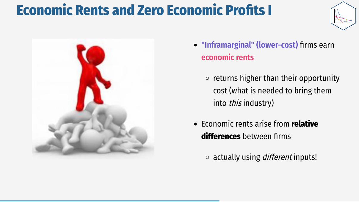
"Inframarginal" (lower-cost) firms earneconomic rents

returns higher than their opportunitycost (what is needed to bring theminto this industry)

Economic rents arise from relativedifferences between firms

actually using different inputs!

Economic Rents and Zero Economic Profits I

Some factors are relatively scarce in theeconomy

(talent, location, secrets, IP, licenses,being first, political favoritism)

Inframarginal firms that use these scarcefactors gain a cost-advantage

It would seem these firms earn profits asother firms have higher costs...

...But what will happen to the pricesfor the scarce factors?

Economic Rents and Zero Economic Profits III

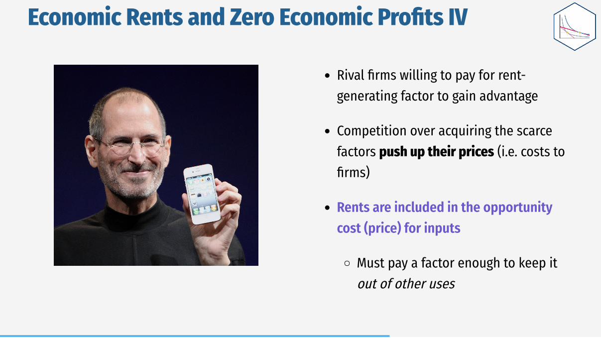
Rival firms willing to pay for rent-generating factor to gain advantage

Competition over acquiring the scarcefactors push up their prices (i.e. costs tofirms)

Rents are included in the opportunitycost (price) for inputs

Must pay a factor enough to keep itout of other uses

Economic Rents and Zero Economic Profits IV

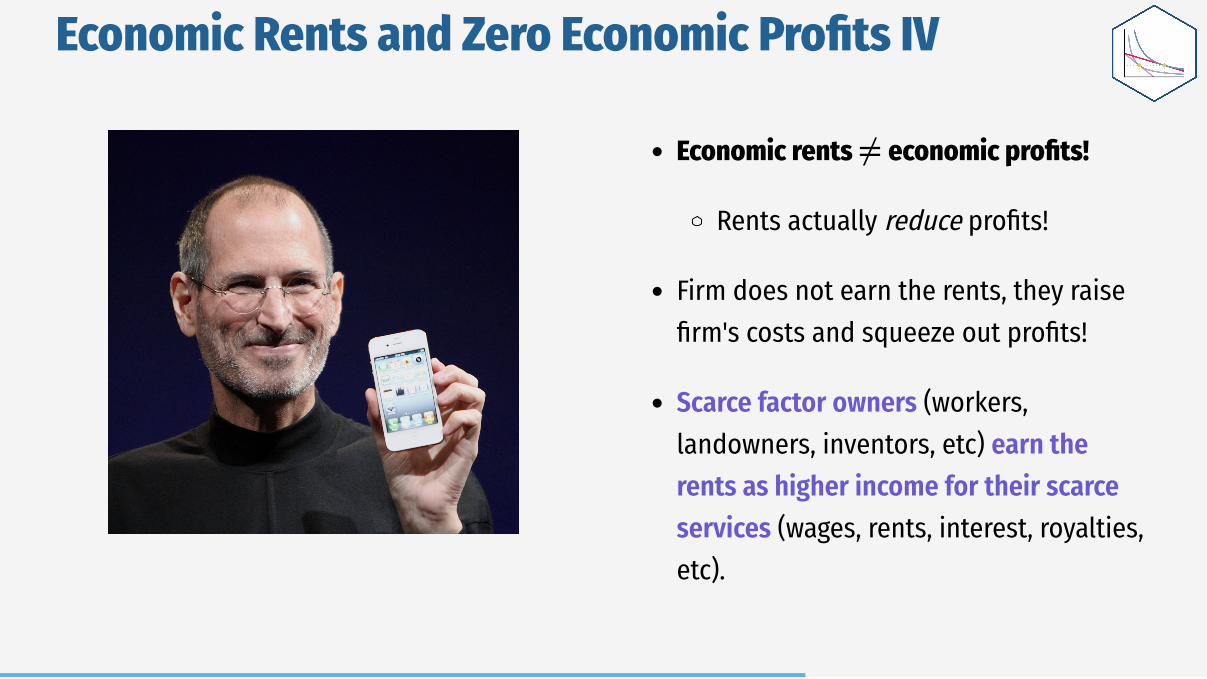
Economic rents economic profits!

Rents actually reduce profits!

Firm does not earn the rents, they raisefirm's costs and squeeze out profits!

Scarce factor owners (workers,landowners, inventors, etc) earn therents as higher income for their scarceservices (wages, rents, interest, royalties,etc).

Economic Rents and Zero Economic Profits IV

≠

Recall "economic" point of view:

Producing your product pulls scarceresources out of other productive uses inthe economy

Profits attract resources to be pulled outof other uses

Losses repel resources to be pulled awayto other uses

Zero profits resources should staywhere they are

Recall: Accounting vs. Economic Point of View

⟹

Supply Functions

Supply function relates quantity to price

Example:

Not graphable (wrong axes)!

Supply Function

q = 2p − 4

Inverse supply function relates price toquantity

Take supply function, solve for

Example:

Graphable (price on vertical axis)!

Inverse Supply Function

p

p = 2 + 0.5q

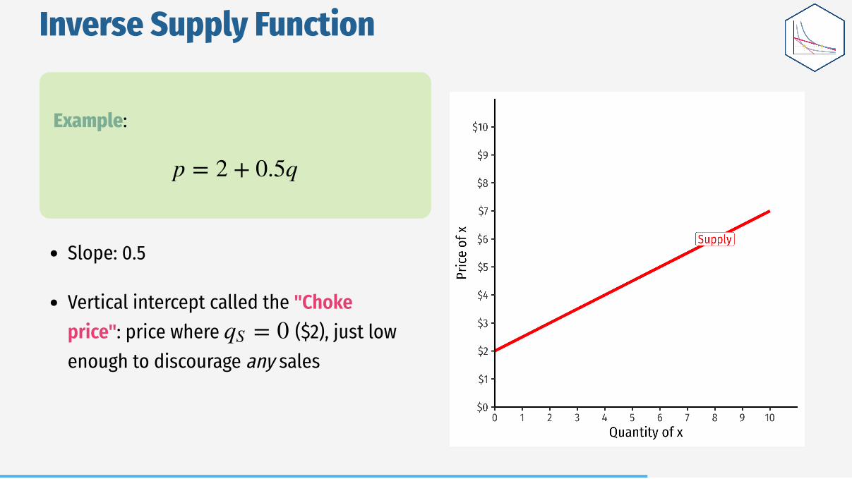
Example:

Slope: 0.5

Vertical intercept called the "Chokeprice": price where ($2), just lowenough to discourage any sales

Inverse Supply Function

p = 2 + 0.5q

= 0qS

Read two ways:

Horizontally: at any given price, howmany units firm wants to sell

Vertically: at any given quantity, theminimum willingness to accept (WTA) forthat quantity

Inverse Supply Function

Price Elasiticity of Supply

Price elasticity of supply measures howmuch (in %) quantity supplied changes inresponse to a (1%) change in price

Price Elasticity of Supply

=ϵ,pqS

%ΔqS

%Δp

Price Elasticity of Supply: Elastic vs. Inelastic

"Elastic" "Unit Elastic" "Inelastic"

Intuitively: Large response Proportionate response Little response

Mathematically:

Numerator Denominator Numerator Denominator Numerator Denominator

A 1% change in More than 1% change in 1% change in Less than 1% change in

=ϵ,pqS

%ΔqS

%Δp

> 1ϵ,pq

s

= 1ϵ,pq

s

< 1ϵ,pq

s

> = <

p qS qS qS

"Inelastic" Supply Curve "Elastic" Supply Curve

Visualizing Price Elasticity of SupplyAn identical 100% price increase on an:

First term is the inverse of the slope ofthe inverse supply curve (that we graph)!

To find the elasticity at any point, weneed 3 things:

�. The price�. The associated quantity supplied�. The slope of the (inverse) supply

curve

Price Elasticity of Supply Formula

= ×ϵq,p

1

slope

p

q

Example

Example: The supply of bicycle rentals in a small town is given by:

�. Find the inverse supply function.

�. What is the price elasticity of supply at a price of $25.00?

�. What is the price elasticity of supply at a price of $50.00?

= 10p − 200qS

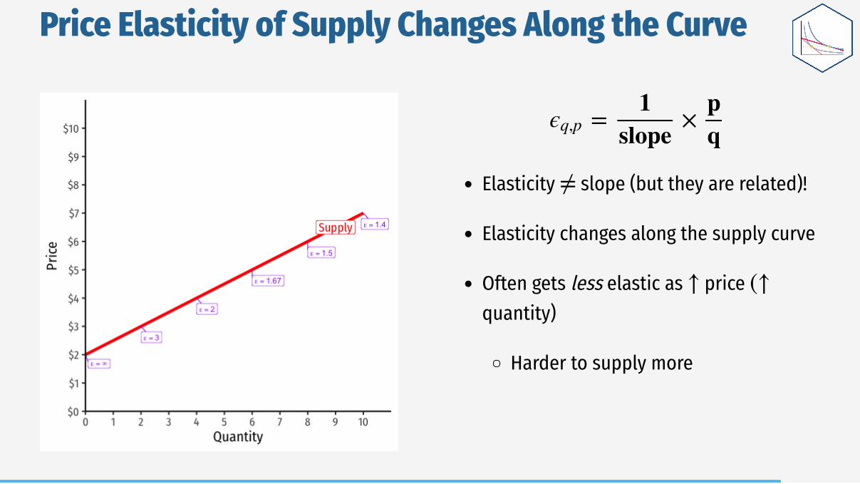
Elasticity slope (but they are related)!

Elasticity changes along the supply curve

Often gets less elastic as price quantity)

Harder to supply more

Price Elasticity of Supply Changes Along the Curve

= ×ϵq,p

1

slope

p

q

≠

↑ (↑

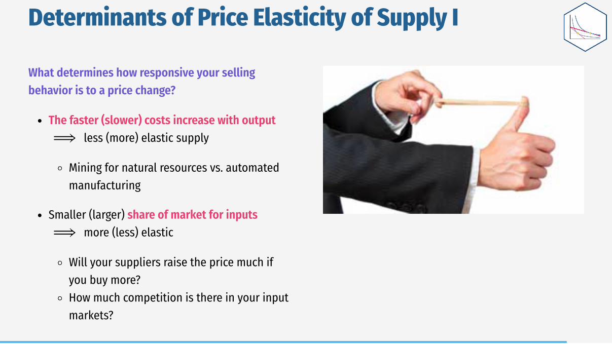
What determines how responsive your sellingbehavior is to a price change?

The faster (slower) costs increase with output less (more) elastic supply

Mining for natural resources vs. automatedmanufacturing

Smaller (larger) share of market for inputs more (less) elastic

Will your suppliers raise the price much ifyou buy more?How much competition is there in your inputmarkets?

Determinants of Price Elasticity of Supply I

⟹

⟹

What determines how responsive yourselling behavior is to a price change?

More (less) time to adjust to pricechanges more (less) elastic

Supply of oil today vs. oil in 10 years

Determinants of Price Elasticity of Supply II

⟹

Price Elasticity of Supply: Examples

Price Elasticity of Supply: Examples

Price Elasticity of Supply: Examples