21st century dam design — advances and adaptations · pdf file21st century dam design...

Hosted by

Black & Veatch Corporation

GEI Consultants, Inc.

Kleinfelder, Inc.

MWH Americas, Inc.

Parsons Water and Infrastructure Inc.

URS Corporation

21st Century Dam Design —

Advances and Adaptations

31st Annual USSD Conference

San Diego, California, April 11-15, 2011

On the CoverArtist's rendition of San Vicente Dam after completion of the dam raise project to increase local storage and provide

a more flexible conveyance system for use during emergencies such as earthquakes that could curtail the region’s

imported water supplies. The existing 220-foot-high dam, owned by the City of San Diego, will be raised by 117

feet to increase reservoir storage capacity by 152,000 acre-feet. The project will be the tallest dam raise in the

United States and tallest roller compacted concrete dam raise in the world.

The information contained in this publication regarding commercial projects or firms may not be used for

advertising or promotional purposes and may not be construed as an endorsement of any product or

from by the United States Society on Dams. USSD accepts no responsibility for the statements made

or the opinions expressed in this publication.

Copyright © 2011 U.S. Society on Dams

Printed in the United States of America

Library of Congress Control Number: 2011924673

ISBN 978-1-884575-52-5

U.S. Society on Dams

1616 Seventeenth Street, #483

Denver, CO 80202

Telephone: 303-628-5430

Fax: 303-628-5431

E-mail: [email protected]

Internet: www.ussdams.org

U.S. Society on Dams

Vision

To be the nation's leading organization of professionals dedicated to advancing the role of dams

for the benefit of society.

Mission — USSD is dedicated to:

• Advancing the knowledge of dam engineering, construction, planning, operation,

performance, rehabilitation, decommissioning, maintenance, security and safety;

• Fostering dam technology for socially, environmentally and financially sustainable water

resources systems;

• Providing public awareness of the role of dams in the management of the nation's water

resources;

• Enhancing practices to meet current and future challenges on dams; and

• Representing the United States as an active member of the International Commission on

Large Dams (ICOLD).

Advanced Analyses with Liquefiable Materials 1369

SEVERAL OBSERVATIONS ON ADVANCED ANALYSES WITH LIQUEFIABLE MATERIALS

Michael H. Beaty1 Vlad G. Perlea2

ABSTRACT

The expected behavior of an embankment dam under earthquake loading is best related to estimates of seismic deformation. Currently, predictions of the magnitude and pattern of seismic deformation are used for both the evaluation of dam safety and the validation of remediation designs for seismically-deficient embankment dams. The US Army Corps of Engineers uses a phased approach for evaluating seismic safety that begins with simple evaluation tools and proceeds, when necessary, to sophisticated analyses. Advanced analyses are generally required for dams of high risk, with significant seismic loads, founded on problem soil, or when simplified evaluations have not resolved seismic concerns. These advanced tools often use non-linear and plasticity-based constitutive models in a two-dimensional finite difference or finite element analysis. One of the major problems with applying these tools to dams with liquefiable soils is the selection of a reliable constitutive model for these problem soils. This paper discusses some of the requirements of such models and the potential effects of modeling assumptions on the predicted seismic deformation. Comparative analyses are performed and the results obtained with advanced models are compared with those from simpler models. The importance of various features on the seismic deformation results is emphasized.

INTRODUCTION

Advances in engineering can be driven by reaction to engineering failures. The 1971 San Fernando Earthquake in California nearly caused a catastrophic failure of the Lower San Fernando Dam due to a massive slide in the upstream embankment. In response to this earthquake, policy was adopted by the Corps of Engineers to help develop and utilize analysis methods that are practical and validated to assure the safety of Corps dams from earthquake hazards. Through the policy set forth in Corps regulations, these analysis methods are integrated into a continual dam safety assurance program for existing projects as well as implemented in new designs.

The fundamental criterion for both the evaluation of dam safety and the validation of the remediation design with respect to earthquake loading is the predicted magnitude and pattern of seismic deformation. Making estimates of deformation often requires sophisticated analysis methods when liquefiable materials are present. Two dimensional finite element or finite difference methods are typically used in conjunction with nonlinear and plasticity-based constitutive models. The primary purpose of this paper is to discuss the importance of the constitutive model selected to represent the liquefiable 1 Principal Engineer, Beaty Engineering LLC, Beaverton, Oregon, 97007 [email protected] 2 Civil Engineer, US Army Corps of Engineers, Sacramento District, Sacramento, California, 95814 [email protected]

21st Century Dam Design — Advances and Adaptations 1370

soils, and to present and discuss analysis predictions based on different constitutive models and modeling assumptions. Some other considerations of advanced modeling of embankments are discussed in Perlea and Beaty (2010).

CONSTITUTIVE MODELS

One of the key aspects in advanced numerical modeling of embankments is the choice of constitutive model. The constitutive model has the task of relating increments of strains to increments of stress. Sophisticated models may include dilative and contractive behavior and will typically address both the elastic response (recoverable strain) and plastic response (irrecoverable strain) response of the material.

General Requirements

Constitutive models have strengths and weaknesses. Many work well only for the specific material types or load paths for which they were developed. The following features should commonly be considered when selecting and using a constitutive model for an advanced analysis:

• The formulation of the constitutive model should adequately address the key features of the anticipated soil behavior. These may include the relationship between shear stiffness and strain, stress-level dependence, generation of pore pressures, and strain softening.

• It should have a sound theoretical basis.

• It should reasonably model the stress-strain and pore pressure generation in monotonic and cyclic laboratory tests. Direct comparisons should be available between numerical simulations and laboratory test data (site specific and/or relevant published information).

• When appropriate, the model should reasonably capture the behavior represented by the empirical relationships for liquefaction triggering and post-liquefaction behavior.

• The selection of input parameters should be reasonably transparent, particularly in cases where direct calibration to laboratory data is not possible.

• Successful use of the model should be documented through back-analysis of case history response.

Due to its critical effect on the deformation predictions, the behavior and calibration of the constitutive model should be clearly documented in an advanced analysis. Significant factors may include stress strain behavior, secant stiffness and hysteretic damping versus cyclic strain, liquefaction resistance versus cyclic stress ratio, liquefaction resistance versus initial confining stress and static shear stress bias, and post-liquefaction behavior including loss of strength and stiffness. Predicted results should be directly compared to laboratory data or published relationships. Results from the back-analysis of case


histories using the selected constitutive models and analytical approach should also be available.

Types of Constitutive Models

The constitutive models typically used in an advanced analysis can be categorized into five primary groups. Each category has a potential and legitimate use. The type of constitutive model selected for each zone is based on the anticipated material behavior and the objective of the analysis.

Linear elastic model: Simple linear elastic models impose a constant proportional relationship between stress increments and strain increments. This model has the advantage of being extremely simple with results that are path independent. However, the model does not consider material yielding and cannot be used to directly model permanent plastic shear strains in elements. It is useful for many rock-like zones where shear failure or a significant nonlinear response is considered unlikely.

Elastic perfectly-plastic models: These models are plasticity-based with a fixed yield or failure surface. Stress increments that occur entirely below the failure surface are considered elastic, although simple hysteretic behavior may be considered. Stress increments that attempt to exceed the strength envelope result in the generation of plastic strains. These models are useful for competent materials where material yielding is possible but effects due to pore pressure generation, pore pressure migration, or cyclic degradation will not be significant. These materials may include compacted embankment shell, impervious core, non-sensitive clays, or unsaturated materials. A common example of a simple elastic-plastic model is the Mohr-Coulomb model found in many numerical analysis programs, including FLAC (Itasca, 2008).

Total stress models: Total stress models are a relatively simple class of constitutive models that simulate the softening of liquefiable elements at the time of triggering. In the simplest formulations, the timing and distribution of liquefaction are manually controlled by the analyst. More sophisticated models use cycle counters based on laboratory data and theoretical formulations to predict the evolution of liquefaction on an element by element basis. Stiffness and strength properties are adjusted in an element to reflect the onset of liquefaction. Although pore pressures are not directly predicted in a true total stress model, the element stiffness may be decreased prior to liquefaction in relation to the anticipated change in pore pressure. Strengths in saturated elements are typically specified as undrained values with a friction angle of zero. The models have the advantage of being simple while still incorporating critical aspects of liquefaction in the analysis. An example of a total stress model used with the computer program FLAC is described by Beaty and Byrne (2008).

Loosely-coupled effective stress models: The element response of an effective stress model is a function of the evolving effective stress state. These models are used primarily for soils subject to changes in effective stress due to cyclic loading. Loosely-coupled models do not directly predict the volumetric strains that lead to pore pressure changes but instead use an independent pore pressure generator. These models evaluate the


predicted cycles of shear stress or shear strain to estimate the corresponding change in pore pressure. Pore pressures are typically adjusted only at the end of each half-cycle of loading. Loosely-coupled models may be extensions of elastic perfectly-plastic models (e.g., Moriwaki et al., 1998; Dawson et al., 2001) or may be based on complex non-linear models (e.g., Finn et al., 1986). Other examples of loosely coupled models include the TARA-3 and TARA-3FL programs (Finn and Yogendrakumar, 1989) and the Finn-Byrne-Itasca model included within FLAC. The TARA programs developed by Prof. Finn have been instrumental in the adoption of advanced analysis techniques for embankments.

Fully-coupled effective stress models: The most sophisticated class of continuum models is the fully-coupled effective stress model. These models directly predict the tendency of soil to dilate or contract in response to each load increment. The resulting volumetric strains are resisted by the stiff pore fluid in saturated elements. This results in the generation or reduction of pore pressure depending on whether the strain is contractive or dilative. Because the stiffness and pore pressure response of these model relies upon the accurate prediction of volumetric strains due to each load increment, these models are often the most difficult to calibrate and verify during normal use. However, the fully-coupled models allow the prediction of soil behavior that most closely resembles that seen in laboratory specimens. The appropriateness of the models for critical structures should be demonstrated through simulation of laboratory element tests, their use in case history and/or centrifuge comparative analyses, and critical evaluation of predicted element response in the dam model.

The effects of pore water flow can often be considered when using a fully-coupled model. Although coupling the groundwater flow and dynamic mechanical response can lead to an extremely complex analysis, the effects of pore pressure migration or dissipation can be significant in some cases. Fully-coupled models allow these potential effects to be better understood through parametric study.

Fully-coupled effective stress models are typically used for liquefiable soils or those that may be affected by changes in pore pressure due to cyclic loading or pore pressure migration. The authors have been involved in studies where several fully-coupled models were successfully used, including the bounding surface hypoplasticity model by Wang (Wang et al., 1990, Wang and Makdisi, 1999), versions of the DYNAFLOW analysis program (Prevost, 2008), and the UBCSAND model as a user-defined subroutine in FLAC (Byrne et al., 2004).

Post-Earthquake Analyses

Much of our understanding of the post-liquefaction strength of sand-like soils is based on the evaluation of case histories where large post-liquefaction deformations were observed. Constitutive models that rely upon a fundamental framework derived from laboratory testing may not directly consider this set of empirical data. While models such as UBCSAND and the Finn-Byrne-Itasca model can induce significant softening or strength loss in elements during the earthquake loading, these softened element may still mobilize more strength than suggested by the empirical database. For this reason, a post-


earthquake stability analysis should always be performed to assess potential deformations due to the selected values of residual strength.

Some practical models directly include the residual strength as part of the potential loading behavior during shaking (e.g., Moriwaki et al., 1998; Dawson et al., 2001; Beaty and Byrne, 2008). In these types of models the strength of liquefied elements is restricted to a maximum of the specified residual strength. These models automatically assess stability using the empirically-derived residual strengths and a post-earthquake stability analysis is generally not needed. However, it is not always clear that application of the residual strength at the instant of liquefaction triggering provides the best estimate of expected response, particularly for cases where the sands are relatively dense.

FLAC MODEL FOR PARAMETRIC STUDY

Analyzed Cross Section

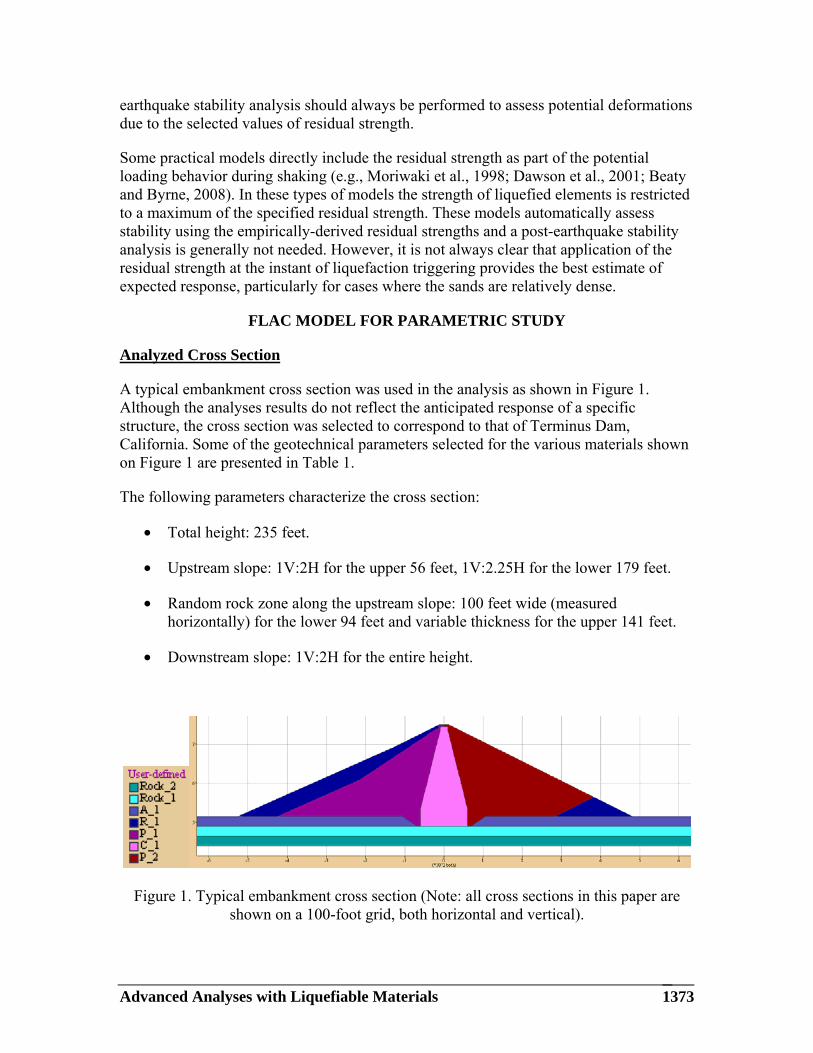
A typical embankment cross section was used in the analysis as shown in Figure 1. Although the analyses results do not reflect the anticipated response of a specific structure, the cross section was selected to correspond to that of Terminus Dam, California. Some of the geotechnical parameters selected for the various materials shown on Figure 1 are presented in Table 1.

The following parameters characterize the cross section:

• Total height: 235 feet.

• Upstream slope: 1V:2H for the upper 56 feet, 1V:2.25H for the lower 179 feet.

• Random rock zone along the upstream slope: 100 feet wide (measured horizontally) for the lower 94 feet and variable thickness for the upper 141 feet.

• Downstream slope: 1V:2H for the entire height.

Figure 1. Typical embankment cross section (Note: all cross sections in this paper are shown on a 100-foot grid, both horizontal and vertical).


The foundation alluvium layer (Zone A_1 on Figure 1) has a thickness of 25 feet. An (N1)60-cs of 10 is assumed to characterize the liquefaction resistance of the alluvium, where (N1)60-cs is the normalized standard penetration resistance corrected to clean sand conditions. A post-liquefaction residual strength, Sr, of 250 psf was also estimated from the assumed (N1)60-cs using the relationship of Idriss and Boulanger (2007). The residual strength applied in any element was not allowed to exceed the initial drained strength of that element. The effect of using Sr rather than a normalized Sr/σ′vo strength was not investigated in this study.

Table 1. Material Properties Consolidated

Drained Consolidated

Undrained Shear Wave

Velocity

Vs Vs1 φ' c' φ c

[(N1)60] and

Residual Strength

Permeability

(ft/day) Material

Symbol (fps) (fps) (deg) (psf) (deg) (psf) Sr (psf) Horiz Vert

Random Rock R_1 1200 45 50 --- --- --- 150 150 Impervious

Core C_1 600 28 50 20 1000 --- 0.1 0.01

Pervious Fill U/S P_1 700 29 50 --- --- --- 100 20

Pervious Fill D/S P_2 1000 29 50 --- --- --- 100 20

Pervious (alluvial)

Foundation*

A_1* 500 28.8 50 --- --- [~10]

250 150 30

Weathered Rock Rock_1 2800 --- --- --- --- --- 25 25

Intact Rock Rock_2 4000 --- --- --- --- --- 25 25 Notes: * Potentially liquefiable layer. VS is the estimated small-strain shear wave velocity. VS1 is the shear wave velocity at a vertical effective stress of 1 atm for stress-dependent soils.

Seismic Loading

The seismic loading was applied to a compliant boundary within the bedrock unit Rock_2. This boundary approximates an elastic half-space of rock and reduces unrealistic reflections from the base of the numerical model. A description of this boundary and its application is described in Mejia and Dawson (2006).

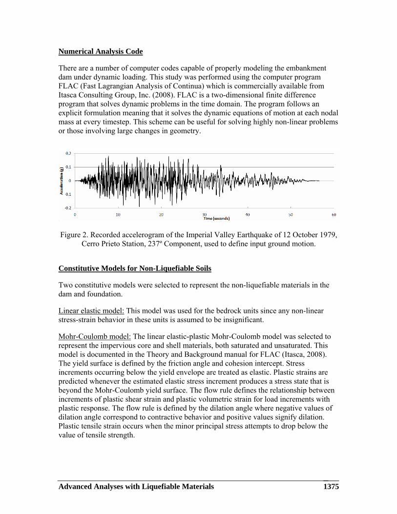
Only horizontal input motions were considered for this study. The selected ground motion was based on work recently completed by URS Corporation (2007) for the Success Dam project in Southern California. The acceleration time series is presented in Figure 2.

Uniform scaling factors were applied to this motion to develop acceleration histories representing four levels of shaking intensity. The scaled records had values of peak ground acceleration (PGA) equal to 0.15g, 0.28g, 0.56g, and 0.75g.


Numerical Analysis Code

There are a number of computer codes capable of properly modeling the embankment dam under dynamic loading. This study was performed using the computer program FLAC (Fast Lagrangian Analysis of Continua) which is commercially available from Itasca Consulting Group, Inc. (2008). FLAC is a two-dimensional finite difference program that solves dynamic problems in the time domain. The program follows an explicit formulation meaning that it solves the dynamic equations of motion at each nodal mass at every timestep. This scheme can be useful for solving highly non-linear problems or those involving large changes in geometry.

Figure 2. Recorded accelerogram of the Imperial Valley Earthquake of 12 October 1979, Cerro Prieto Station, 237º Component, used to define input ground motion.

Constitutive Models for Non-Liquefiable Soils

Two constitutive models were selected to represent the non-liquefiable materials in the dam and foundation.

Linear elastic model: This model was used for the bedrock units since any non-linear stress-strain behavior in these units is assumed to be insignificant.

Mohr-Coulomb model: The linear elastic-plastic Mohr-Coulomb model was selected to represent the impervious core and shell materials, both saturated and unsaturated. This model is documented in the Theory and Background manual for FLAC (Itasca, 2008). The yield surface is defined by the friction angle and cohesion intercept. Stress increments occurring below the yield envelope are treated as elastic. Plastic strains are predicted whenever the estimated elastic stress increment produces a stress state that is beyond the Mohr-Coulomb yield surface. The flow rule defines the relationship between increments of plastic shear strain and plastic volumetric strain for load increments with plastic response. The flow rule is defined by the dilation angle where negative values of dilation angle correspond to contractive behavior and positive values signify dilation. Plastic tensile strain occurs when the minor principal stress attempts to drop below the value of tensile strength.


Constitutive Models for Liquefiable Soils

Three models were used in the parametric study to represent the behavior of the liquefiable alluvium layer.

UBCSAND: This fully-coupled effective stress model was developed at the University of British Columbia by Prof. Peter Byrne and is described in Byrne et al. (2004). The version used in this study includes some additional modifications to improve the behavior of the model under various initial shear stress conditions (Beaty, 2009). This model is the most sophisticated of the three models evaluated in the current study.

UBCSAND can be viewed as an expanded version of the Mohr-Coulomb model. Instead of a fixed yield surface used in the standard Mohr-Coulomb model, the yield surface in UBCSAND is allowed to evolve or harden in response to the loading history. This allows the prediction of hysteretic behavior as plastic behavior may occur at loading increments below the strength envelope. Hardening of the yield surface is based on a hyperbolic relationship between the plastic shear strain and the stress ratio. The flow rule is based on the stress ratio, where stress states below the constant volume friction angle are contractive and stress states above are dilative. The modified version of UBCSAND used in this study improves the prediction of liquefaction in cases where static bias effects are important.

Finn-Byrne-Itasca model: This loosely-coupled effective stress model is included in FLAC as described in the Optional Features manual from Itasca (2008). Although this model is based upon the work of Professors Liam Finn and Peter Byrne from the University of British Columbia, Canada (Martin et al., 1975; Byrne, 1991), the specific implementation of the model in FLAC was formulated by Itasca. This method relies upon a relationship between half cycles of shear strain and increments of volumetric strain that was derived from a set of laboratory element tests. Increments of volumetric strain are related to the shear strain amplitude of a loading cycle, the previously-accumulated volumetric strain, and relative density.

An approximate logic has been developed by Itasca to identify shear strain reversals in general two-dimensional loading. Once a half cycle of shear strain has occurred its amplitude is used to estimate the corresponding plastic volumetric strain increment. The effects of this volumetric strain are applied through an equivalent drop in effective stress within an element as determined by the volumetric strain increment and the elastic stiffness. This stress change causes an imbalance in the total stresses on the element and induces the element to contract until the resulting increase in pore pressure and changes in effective stress brings the element into equilibrium. This relationship is used in conjunction with the standard Mohr-Coulomb model. The primary effect of the pore pressures generated by the Finn-Byrne-Itasca model is to reduce the effective stress and the corresponding frictional strength that can be mobilized.

Mohr-Coulomb model (gravity only): The Mohr-Coulomb model can be used to perform a post-earthquake stability analysis using a total stress formulation. The extent of liquefaction is first estimated and the residual strength is assigned to liquefied zones in


order to approximate the degradation of strength and stiffness anticipated in these zones during the earthquake. Only loading from gravity is included in the post-earthquake analysis and the inertial response to earthquake motions is not considered. This approach is generally considered useful to evaluate the potential for large displacements related to flow slides.

Pre-Dynamic Static Equilibrium

The initial static analysis was performed in stages that simulate a simplified construction sequence. The Mohr-Coulomb model was used with stress-dependent stiffness properties in all soil zones. The construction process was simulated by performing the following analysis steps: 1) initial stress state of the foundation without any embankment, 2) excavation for the impervious core, 3) sequential construction of the dam in stages, and 4) seepage analysis to represent reservoir filling. Since FLAC solves even static problems using a dynamic formulation, the amount of material included in each construction stage was relatively small, e.g. one 5-foot layer of elements added between solution steps.

Although the detailed stress distribution within an embankment is largely unknown, and many reasonable stress states can be developed that satisfy equilibrium, this procedure is considered reasonable for developing an estimate of the initial stress state in the current study. Selected predictions of initial state are shown on Figures 3 through 6.

CONSTITUTIVE MODEL AND MODELING APPROACH

Each constitutive model was used to estimate the behavior of the liquefiable layer and the resulting response of the embankment. Selected results from each analysis are summarized below. The material parameters listed in Table 1 were used except as indicated. Pore water flow was not considered in this parametric study although the effects of the fluid stiffness were directly included in the element response.

Seismic Deformation using UBCSAND model

Analysis Procedure: The numerical model was converted to dynamic analysis conditions once the initial static analysis was complete. These steps are summarized below:

• The properties of the Mohr-Coulomb and elastic zones were adjusted to address the anticipated dynamic response of the elements. This included the specification of dynamic stiffness values.

• The UBCSAND model was assigned to the potentially liquefiable unit RA_1. Generic constitutive model parameters indexed to (N1)60cs estimates were used to


•

Figure 3. Steady state condition for full pool. Pore pressure units are lb/ft2. Phreatic surface shown by dark blue line.

Figure 4. Effective vertical stresses in lb/ft2.

Figure 5. Effective horizontal stress in lb/ft2.

Figure 6. Shear stress on horizontal/vertical planes in lb/ft2.


define the material response. These parameters have been calibrated to achieve reasonable agreement to accepted relationships for cyclic resistance ratio, effect of static shear bias (Kα), and effect of initial confining stress (Kσ).

• Approximate levels of viscous (Rayleigh) damping were assigned: 0.5% of critical was assigned to the elastic bedrock zones, 3% to the Mohr-Coulomb zones, and 1% to the UBCSAND zones to address numerical stability issues and to provide a nominal amount of damping during elastic loading and unloading cycles. UBCSAND includes hysteretic damping through its modeling of non-linear behavior.

The damping assigned to the Mohr-Coulomb zones is a low estimate, particularly for the stronger earthquake motions, but was selected for use in these comparative analyses to speed solution times. It should be remembered that the viscous damping applies only to the elastic response. Energy loss through hysteretic damping is naturally included whenever plastic shear strains are predicted.

• Free-field boundaries were assigned to the left and right boundaries of the model, and a compliant (non-reflecting) boundary was assigned to the base of the model. This compliant boundary requires the input acceleration history to be converted into an equivalent shear stress history before its application.

• The earthquake motion was applied to the base of the model and the dynamic response analysis performed through the end of the ground motion.

• The analysis was continued an additional five seconds without any input motion to permit additional decay of the embankment response.

• A post-earthquake stability analysis was performed by identifying zones that liquefied during the seismic loading and then assigning strength parameters consistent with the post-earthquake residual strength. Liquefied zones were identified by evaluating the peak excess pore pressure ratio ru, where ru is defined as 1 – σ'v/σ'v0, σ'v is the minimum vertical effective stress and σ'v0 is the initial vertical effective stress. Zones with a maximum ru greater than 0.7 were considered subject to liquefaction behavior. The zones identified as liquefied using this criterion should be evaluated for reasonableness, particularly when small pockets of non-liquefaction are identified within larger zones of liquefiable soils or when zones identified as non-liquefied have experienced large shear strains.

The constitutive model for the liquefied zones was converted to Mohr-Coulomb, the strength set equal to the residual strength, and a softened shear modulus equal to 0.1×Sr assigned. The strength in all zones was limited to a maximum value equal to the estimated drained strength. This is particularly important for zones using the UBCSAND model where dilation, with a corresponding drop in pore pressure, may allow larger strengths to develop than would be customary in a


post-earthquake analysis. The analysis is continued until equilibrium is achieved and the displacements stabilize.

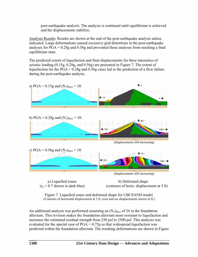
Analysis Results: Results are shown at the end of the post-earthquake analysis unless indicated. Large deformations caused excessive grid distortions in the post-earthquake analyses for PGA = 0.28g and 0.56g and prevented these analyses from reaching a final equilibrium state.

The predicted extent of liquefaction and final displacements for three intensities of seismic loading (0.15g, 0.28g, and 0.56g) are presented in Figure 7. The extent of liquefaction for the PGA = 0.28g and 0.56g cases led to the prediction of a flow failure during the post-earthquake analysis.

a) PGA = 0.15g and (N1)60cs = 10:

b) PGA = 0.28g and (N1)60cs = 10:

(displacements still increasing) c) PGA = 0.56g and (N1)60cs = 10:

(displacements still increasing) a) Liquefied zones b) Deformed shape (ru > 0.7 shown in dark blue) (contours of horiz. displacement at 5 ft)

Figure 7. Liquefied zones and deformed shape for UBCSAND model. (Contours of horizontal displacement at 5 ft; crest and toe displacements shown in ft.)

An additional analysis was performed assuming an (N1)60cs of 24 in the foundation alluvium. This revision makes the foundation alluvium more resistant to liquefaction and increases the estimated residual strength from 250 psf to 2500 psf. This analysis was evaluated for the special case of PGA = 0.75g so that widespread liquefaction was predicted within the foundation alluvium. The resulting deformations are shown in Figure

6

14 5

40+

30+ 100+

70+

50+ 100+


8. The residual strength was sufficiently high in this case for the analyses to reach a stable geometry at the end of the post-earthquake phase although the predicted displacements were still very large. The relative importance of the inertial and post-earthquake phase can be seen by comparing the two plots in Figure 8. The crest settlement at the end of shaking was 36 feet and at the end of the post-earthquake analysis it increased to 59 feet.

a) End of shaking b) End of post-earthquake analysis

Figure 8. Deformation predictions for UBCSAND, (N1)60cs = 24, and PGA = 0.75g. (Contours of horizontal displacement at 5 ft, crest and toe displacements shown in ft.)

Analysis Discussion: This set of analyses suggest several conclusions for this test embankment: a) predicted displacements are relatively small if liquefaction is limited, and b) large deformations will occur if sufficient liquefaction is predicted even for the case with (N1)60cs = 24, and c) large deformations can be caused both by inertial response during shaking as well as gravity acting on the degraded structure, and d) the post-earthquake analysis can significantly increase the estimate of displacements. The predicted extent of liquefaction appears to be a critical aspect of the analysis for the assumed structure and properties.

Seismic Deformation using FLAC Finn-Byrne-Itasca Model

Analysis Procedure: The numerical model was converted to dynamic analysis conditions once the initial static analysis was complete. This process was identical to that used for the UBCSAND analyses except as indicated below:

• The Finn-Byrne-Itasca model was assigned to unit RA_1. The coefficients for the Finn-Byrne-Itasca model were selected following the guidelines summarized in the FLAC manual and based on the work of Prof. Byrne (1991). These coefficients are expressed as a function of (N1)60cs. Drained strength parameters were used as specified in Table 1. Stress-dependent stiffness parameters were assigned to the alluvium. The shear modulus was set equal to 30% of the estimated Gmax and a Poisson’s ratio of 0.20 was used to approximate the bulk modulus for small strain, drained loading. Drained strength parameters were assigned to the RA_1 unit with a dilation angle of zero.

• Rayleigh viscous damping equal to 3% of critical was assigned to unit RA_1 to maintain general consistency with the approach used in the UBCSAND analysis.

35

17 23

60

20 55


• A post-earthquake analysis was performed using the same process as adopted for the UBCSAND analysis. The direct application of Finn-Byrne-Itasca model as described in the FLAC manual (Itasca, 2008) does not discuss the merits or techniques of a post-earthquake analysis, although such an analysis is typically prudent.

Analysis Results: Figure 9 presents results from the Finn-Byrne-Itasca model analysis in terms of zones of liquefaction and final deformed shape. Figure 10 compares the difference in displacements at the end of shaking and end of the post-earthquake analysis.

PGA = 0.15g and (N1)60cs = 10:

PGA = 0.28g and (N1)60cs = 10:

PGA = 0.56g and (N1)60cs = 10:

a) Liquefied zones b) Deformed shape (shown in dark blue) (contours of horizontal displacement at 5 ft)

Figure 9. Liquefied zones and deformed shape at end of post-earthquake analysis

for Finn-Byrne-Itasca model. (Contours of horizontal displacement at 5 ft, crest and toe displacements shown in ft.)

6

5 3

60

18 90

10 8

14


PGA = 0.15g and (N1)60cs = 10:

PGA = 0.28g and (N1)60cs = 10:

PGA = 0.56g and (N1)60cs = 10:

a) End of shaking b) End of post-earthquake analysis

Figure 10. Deformed shape at end of shaking and end of post-earthquake analysis for Finn-Byrne-Itasca model.

(Contours of horizontal displacement at 5 ft, crest and toe displacements shown in ft.)

Analysis Discussion: Significant differences are seen between the results from the Finn-Byrne-Itasca and UBCSAND analyses. It is evident that the Finn-Byrne-Itasca approach predicts a significantly smaller extent of liquefaction than the UBCSAND analysis for the adopted material properties, particularly beneath the downstream shell and for the PGA = 0.56g analysis. The predicted displacements are correspondingly smaller.

One aspect of using the Finn-Byrne-Itasca approach is worth further discussion. The Finn-Byrne-Itasca equations as described in the FLAC manual essentially provide the flow rule for the model (i.e., it relates shear strain increments to contractive increments of plastic volumetric strain). In Byrne’s 1991 paper, he demonstrated that this flow rule gives reasonable results for a selected loading condition for a particular constitutive model and stiffness assumptions. The behavior using a constitutive model and stiffness assumptions differing from those of Byrne (1991) should be confirmed before use.

The selection of stiffness parameters for a Mohr-Coulomb model typically begins with Gmax. Estimates of Gmax are often made from shear wave velocity estimates or approximated from penetration test results. The dynamic shear modulus is estimated by applying a modulus reduction factor to Gmax and the bulk modulus can be derived from

5 3

18 90

10 8

3 3

14

30

25

60

6

14

6

5

11

8


Gmax by assuming a Poisson’s ratio. This was the approach used in these parametric analyses. However, since the Finn-Byrne-Itasca model relies upon strain estimates, and many analyses are essentially stress-controlled, the proper choice of stiffness parameters is integral to its proper use. For example, the ratio of the shear modulus to bulk modulus of the soil skeleton can have a significant impact on the pore pressures predicted by the Finn-Byrne-Itasca model in stress-controlled cases.

It is highly recommended when using the Finn-Byrne-Itasca model that the behavior be verified for the stress and loading conditions and the stiffness parameters to be used in the model. This is typically done by simulating laboratory element tests such as a direct simple shear and comparing the predicted response to anticipated results. This type of detailed calibration may have led to better agreement between the Finn-Byrne-Itasca and UBCSAND results, and could have greatly increased confidence in the Finn-Byrne-Itasca predictions.

Seismic Deformation using Mohr-Coulomb Model (gravity only)

Analysis Procedure: The Mohr-Coulomb constitutive model can be used to perform simplified or initial evaluations of potential deformations. The primary assumption of this approach is that seismic deformations due to liquefaction are primarily caused by gravity forces acting on the weakened structure and not the inertial response during strong shaking. The analysis process is very similar to the post-earthquake evaluation performed as part of the UBCSAND analysis approach.

• The liquefaction of critical zones is first estimated using a separate technique. This may include the simplified method as described by Youd, Idriss et al. (2001) or equivalent linear analyses such as Quad4m (Hudson et al., 1994). The extent of liquefaction is identified with due consideration given to approximations in the analysis method. For this parametric study, the liquefaction extent predicted in the UBCSAND analyses was used to allow for direct comparison between the results.

• Following completion of the static analysis, appropriate undrained strength parameters are assigned to all zones. Residual strengths are used in any zone that is considered liquefied. Strength parameters in non-liquefied zones should generally consider the effect of partial loss of effective stress due to pore pressure generation. For these simple parametric analyses, the effects of pore pressure changes in non-liquefied zones were assumed to be nominal. The strength of all zones is typically limited to the minimum of the drained strength, undrained strength, and the residual strength (for liquefied zones).

Analysis Results: Figure 11 compares the displacements predicted from the UBCSAND analyses with estimates from the Mohr-Coulomb (gravity only) analyses for three loading cases. The PGA = 0.56g case with (N1)60cs = 10 is not shown since each analysis predicted a flow slide. The predicted displacements from the Mohr-Coulomb evaluation are noticeably less than those from the UBCSAND evaluation in each case.


PGA = 0.15g with (N1)60cs = 10:

PGA = 0.28g with (N1)60cs = 10:

(final equilibrium not achieved) PGA = 0.75g with (N1)60cs = 24:

a) UBCSAND b) Mohr-Coulomb (gravity only)

Figure 11. Deformed shape at end of post-earthquake analysis from UBCSAND and Mohr-Coulomb (gravity only) analyses.

(Contours of horizontal displacement at 5 ft, crest and toe displacements shown in ft.)

Analysis Discussion: There are distinct differences in both the displacement magnitudes and patterns between the UBCSAND and Mohr-Coulomb (gravity-only) predictions. For example, the UBCSAND analysis for PGA = 0.75g shows a more distributed shear pattern within the embankment with significant deformations occurring within both the upstream and downstream shells. The shear behavior in the Mohr-Coulomb analysis is more localized and confined to movements in the downstream direction. Although both analyses show large crest deformations, the general behavior is significantly different.

The disparities in displacement magnitudes may be large enough in some cases to produce differing conclusions regarding dam safety. The difference between the two analyses is likely due to the inertial response of the dam acting on the weakened alluvial soils. This response is directly included in the UBCSAND analysis but excluded from the gravity-only approach. One other factor that has an influence on this comparison is the effect of pore pressures generated in non-liquefied zones. This is part of the UBCSAND analysis but was not included in this preliminary Mohr-Coulomb evaluation.

0.0

6 0.7

16+

13+ 85+

35

0 30

60

20 55

6

14 5

40+

30+ 100+


This comparison demonstrates the conclusion that Mohr-Coulomb (gravity only) analyses are generally useful for identifying cases of large displacement. Although the sophistication of a FLAC analysis can provide benefits over a traditional limit equilibrium analysis, these benefits are not always worth the additional effort and time that is required. The gravity-only analysis is generally insufficient if it demonstrates moderate to small displacements as these cases can be significantly impacted by inertial response. In additional, large displacements magnitudes and patterns from a gravity-only analysis may only approximate those from a more sophisticated analysis.

Seismic Deformation using Mohr-Coulomb Model (no liquefaction)

Analysis Procedure: A substantial portion of the displacement in the previous analyses was found to occur due to inertial response during strong ground shaking. An additional analysis was performed to estimate the importance of liquefaction modeling to the prediction of these displacements. This was done by assigning the Mohr-Coulomb model to the alluvium layer but without any modeling of pore pressure generation. In essence, the Finn-Byrne-Itasca analysis was repeated with the same material properties except the computation of plastic volumetric strain was not performed.

Analysis Results: Predictions of final displaced shape are shown on Figure 12. The results from the Mohr-Coulomb (no liquefaction) and the Finn-Byrne-Itasca results at the end of earthquake shaking are shown to provide a direct comparison for the three levels of earthquake loading.

Analysis Discussion: The predicted deformations for the Mohr-Coulomb analysis tend to be relatively symmetric about the crest. The upstream and downstream toes appear to move about the same distance in opposite directions, and the crest settles vertically. This is likely a function of the earthquake record but suggests the response for this cross section is relatively balanced in the absence of liquefaction.

The displacements for the Mohr-Coulomb case are not as large as for the Finn-Byrne-Itasca or UBCSAND cases, but the displacements are still substantial for the stronger motions.

Discussion on Constitutive Model and Modeling Approach

Table 2 summarizes the final displacement estimates for the three seismic loading levels and the four modeling approaches. General observations regarding the predictions of displacements and liquefaction extent include the following:

• The largest deformations are predicted using the UBCSAND model and the smallest are from the Mohr-Coulomb analysis with no liquefaction.

• The UBCSAND analyses predict substantially more displacement than the Finn-Byrne-Itasca approach. This appears related to the predicted extent of liquefaction. The difference in displacement predictions is significant enough to impact an evaluation of safety.


PGA = 0.15g and (N1)60cs = 10:

PGA = 0.28g and (N1)60cs = 10:

PGA = 0.56g and (N1)60cs = 10:

a) Mohr-Coulomb (no liquefaction) b) Finn-Byrne-Itasca Model

Figure 12. Deformed shape at end of earthquake shaking from Mohr-Coulomb (no liquefaction) and Finn-Byrne-Itasca analyses. (Contours of horizontal displacement at 5 ft, crest and toe displacements shown in ft.)

Table 2. Final displacement estimates in feet PGA = 0.15g PGA = 0.28g PGA = 0.56g

Model U/S Toe Crest D/S

Toe U/S Toe Crest D/S

Toe U/S Toe Crest D/S

Toe UBCSAND 14 6 5 30+ 40+ 100+ 50+ 70+ 100+ Finn-Byrne-Itasca 5 6 3 10 14 8 18 60 90 Mohr-Coulomb - gravity only - no liquefaction

6

0.8

0.0 1.6

0.7 0.6

13+

3

16+

6

85+ 2.4

-- 8

-- 16

-- 8

3 3

14 25

6 8

0.8 0.6

8

16

8

30

5

11

3

1.6

6

2.4


• As shown by the comparisons in Figure 8 and Figures 10, including a post-earthquake analysis using estimates of residual strength in liquefied elements can be significant to the final displacement estimates.

• Mohr-Coulomb (gravity only) analyses may be useful for identifying cases of large displacement. Although the sophistication of a FLAC analysis can provide benefits over a traditional limit equilibrium analysis, these benefits are not always worth the additional effort and time that is required. The displacements patterns and magnitudes from a gravity-only FLAC analysis may not always represent a best estimate of those anticipated during a large earthquake event. The gravity-only analysis is generally insufficient in evaluating embankment safety if it predicts moderate to small displacements.

• Due to the size of the dam, large deformations will occur if extensive liquefaction is predicted even when the alluvium is assigned an (N1)60cs of 24. This highlights the importance of making a reliable estimate of the extent of liquefaction. A Quad4 analysis can be useful in evaluating the predicted extent of liquefaction.

• A somewhat different set of comparisons and conclusions may have been reached if a normalized Sr/σ′vo model was used since residual strengths in the interior of the dam would have been higher than those used in this study. There would be a tendency for the larger movements to occur closer to the face of the dam.

• Large displacement can be predicted in the absence of liquefaction if relatively low strengths are used in combination with large seismic loads. For this section, most of the embankment and alluvium units were assigned a friction angle of only 28° to 29° with a cohesion intercept of 50 psf. Crest settlements of 16 feet were predicted for the PGA = 0.56g case using these strength assumptions even without liquefaction.

LAYER THICKNESS FOR LIQUEFIABLE ZONE

The dam model described above was used to evaluate the effect of the thickness of a liquefiable layer. This directly evaluates the layer thickness and indirectly the effect of mesh density across the liquefiable layer.

Each row of elements within the alluvium layer is 5 feet high. The analysis was run assuming a different number of rows were liquefiable, from 0 to 5. The cross section used in the parametric studies described above included 5 rows of elements within the liquefiable layer.

The excess pore pressures were monitored at the center of the layer during each analysis. The liquefiability of the alluvium was described by an (N1)60-cs of 20, a value selected to limit deformations and restrict excessive distortion of the mesh. The UBCSAND model and modeling approach were used for the liquefiable alluvium. In all cases the seismic loading was described by the accelerogram shown on Figure 2 scaled to a PGA = 0.56g. This intensity of shaking was selected for obtaining complete liquefaction in the entire


alluvial layer when the 5-row variant was assumed. The analysis was run in both “flow on” and “flow off” (undrained) conditions during the earthquake analysis.

Parametric Study Results

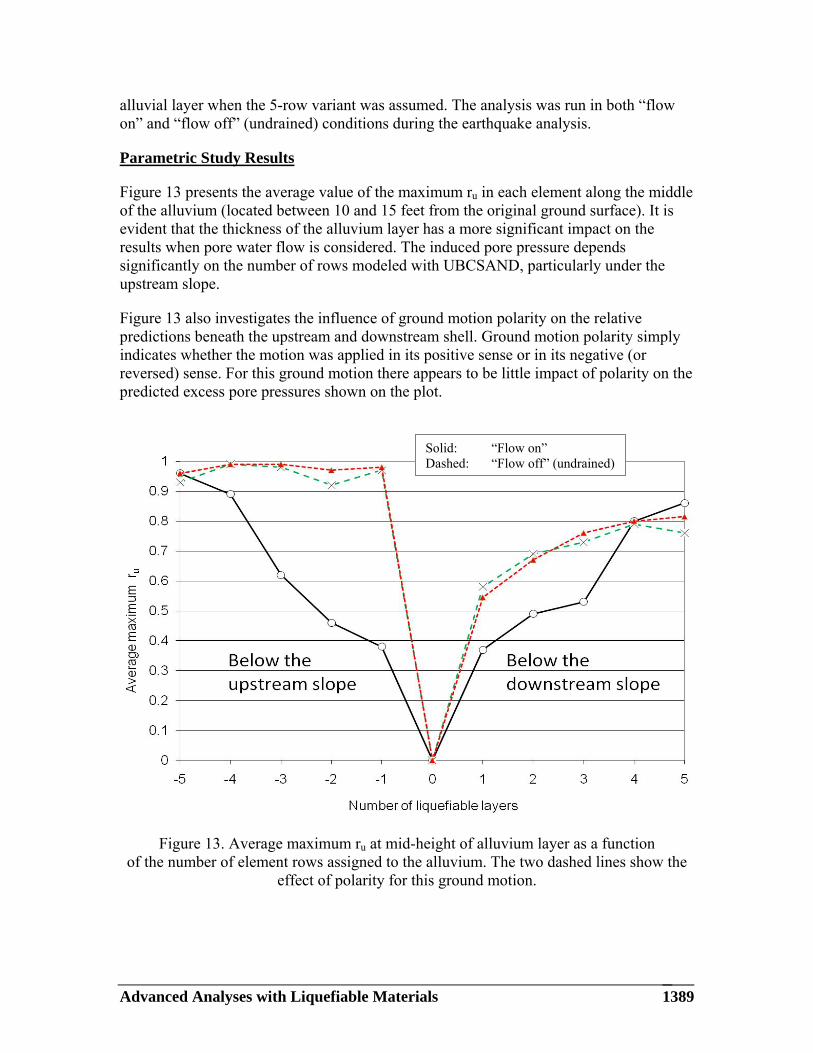
Figure 13 presents the average value of the maximum ru in each element along the middle of the alluvium (located between 10 and 15 feet from the original ground surface). It is evident that the thickness of the alluvium layer has a more significant impact on the results when pore water flow is considered. The induced pore pressure depends significantly on the number of rows modeled with UBCSAND, particularly under the upstream slope.

Figure 13 also investigates the influence of ground motion polarity on the relative predictions beneath the upstream and downstream shell. Ground motion polarity simply indicates whether the motion was applied in its positive sense or in its negative (or reversed) sense. For this ground motion there appears to be little impact of polarity on the predicted excess pore pressures shown on the plot.

Figure 13. Average maximum ru at mid-height of alluvium layer as a function of the number of element rows assigned to the alluvium. The two dashed lines show the

effect of polarity for this ground motion.

Solid: “Flow on” Dashed: “Flow off” (undrained)


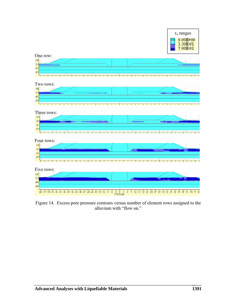
The dependence of liquefaction on alluvium layer thickness is further demonstrated in Figures 14 and 15. These plots show contours of maximum excess pore pressure ru for each of the analysis cases. The actual extent of liquefaction prediction is somewhat greater than shown in these figures, particularly for the 1 layer analysis, due to some smoothing used in the contouring process. It is clear that there is a significant impact of both layer thickness and flow conditions on the predicted extent of liquefaction.

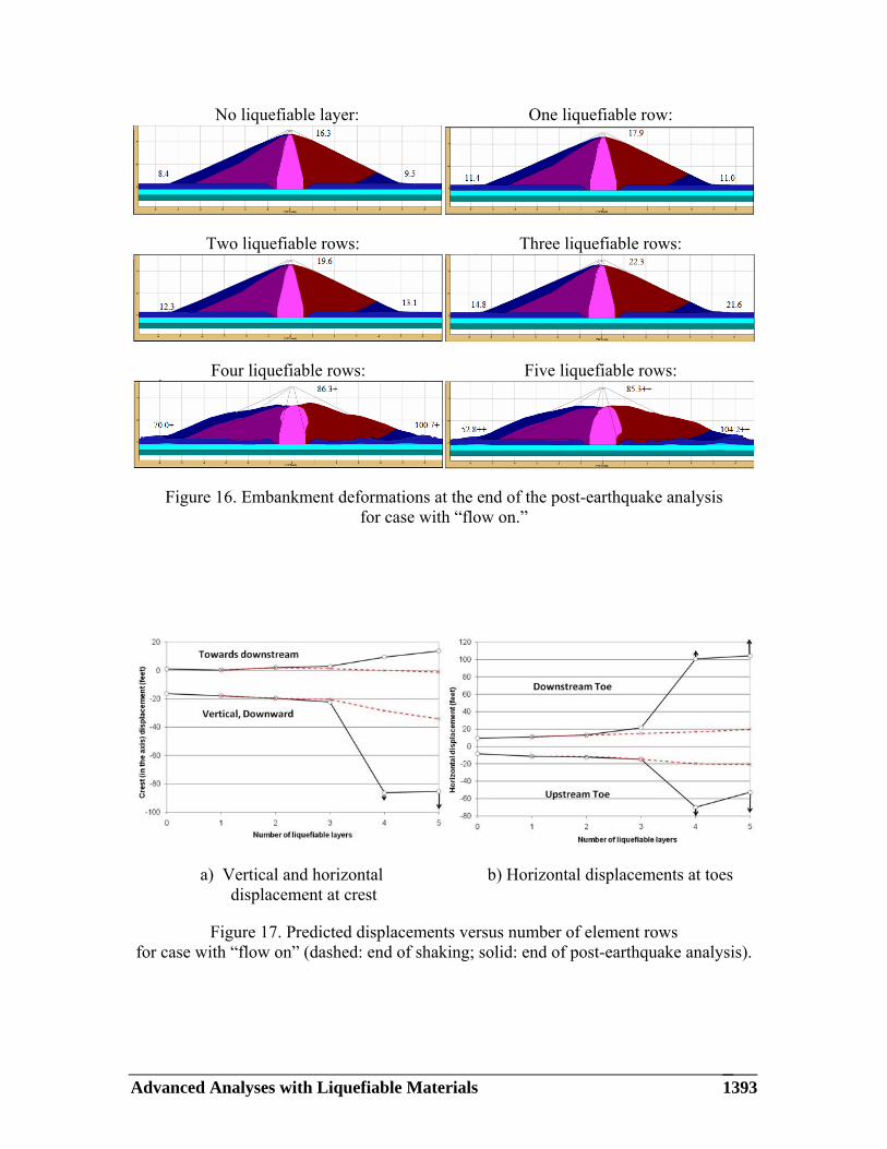
The assumed number of liquefiable rows also has a significant impact on the computed seismic deformation. The deformed shapes at the end of the post-earthquake analysis for cases where fluid flow is included are shown in Figure 16. There is a significant difference in the final displacement conditions between the use of 3 or fewer rows of elements and 4 or more rows. The extent of liquefaction predicted for the cases with 4 or 5 rows of elements within the alluvium produce flow slide conditions. The grid in these cases is continuing to deform at the end of analysis with a slight tendency for stabilization in the “four rows” case but with high final velocities in the “five rows” case.

The displacement data are also plotted in Figures 17 and 18. Solid (black) lines represent the predictions at the end of the post-earthquake analysis and broken (red) lines correspond to the end of shaking, the difference between the lines being the displacements occurring during the post-liquefaction analysis. Figure 17 shows the predictions for the “flow on” case. Figure 18 provides a direct comparison of the “flow on” and “flow off” results.

The post-earthquake analysis had little impact on the displacements when 3 or fewer rows were used, but it was essential to the identification of displacements in the 4 or 5 row cases. Although a thicker liquefiable layer may generate a different seismic response and lead to larger displacements, the brittle response observed between the “3 row” and “4 row” cases provides a significant caution. Although mesh density was not directly evaluated in this study, modeling liquefiable layers with too coarse a mesh may give unexpected results.

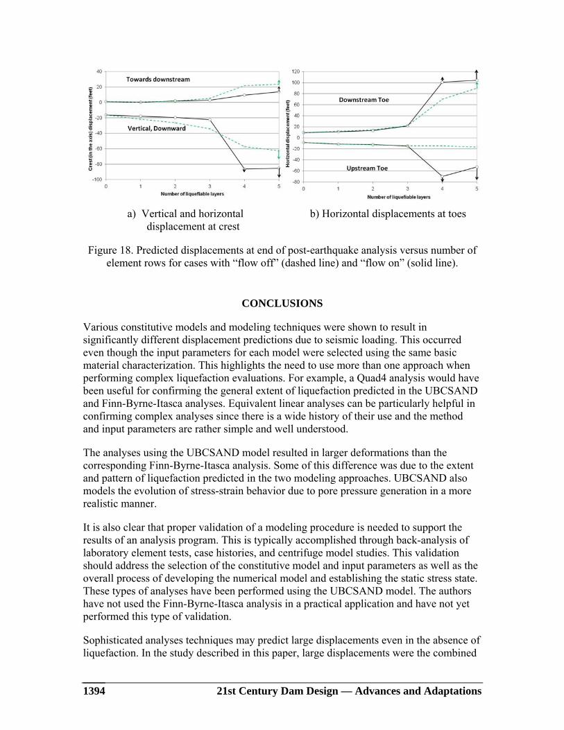
The “flow on” versus “flow off” formulation also had a significant effect on the computed displacements. At the crest, the “flow off” results tended to produce larger displacements except for the two cases where flow slides were predicted. Pore water flow had little impact on the predicted toe displacements except for the two cases that resulted in flow slides. For these cases, the “flow off” results were significantly larger. Although a clear trend was not seen, these observations point to the importance of including pore water flow into a typical parametric study.


One row:

Two rows:

Three rows:

Four rows:

Five rows:

Figure 14. Excess pore pressure contours versus number of element rows assigned to the alluvium with “flow on.”

ru ranges


One row:

Two rows:

Three rows:

Four rows:

Five rows:

Figure 15. Excess pore pressure contours versus number of element rows assigned to the alluvium with “flow off” (undrained conditions).

ru ranges


No liquefiable layer: One liquefiable row:

Two liquefiable rows: Three liquefiable rows:

Four liquefiable rows: Five liquefiable rows:

Figure 16. Embankment deformations at the end of the post-earthquake analysis for case with “flow on.”

a) Vertical and horizontal b) Horizontal displacements at toes displacement at crest

Figure 17. Predicted displacements versus number of element rows for case with “flow on” (dashed: end of shaking; solid: end of post-earthquake analysis).


a) Vertical and horizontal b) Horizontal displacements at toes displacement at crest

Figure 18. Predicted displacements at end of post-earthquake analysis versus number of element rows for cases with “flow off” (dashed line) and “flow on” (solid line).

CONCLUSIONS

Various constitutive models and modeling techniques were shown to result in significantly different displacement predictions due to seismic loading. This occurred even though the input parameters for each model were selected using the same basic material characterization. This highlights the need to use more than one approach when performing complex liquefaction evaluations. For example, a Quad4 analysis would have been useful for confirming the general extent of liquefaction predicted in the UBCSAND and Finn-Byrne-Itasca analyses. Equivalent linear analyses can be particularly helpful in confirming complex analyses since there is a wide history of their use and the method and input parameters are rather simple and well understood.

The analyses using the UBCSAND model resulted in larger deformations than the corresponding Finn-Byrne-Itasca analysis. Some of this difference was due to the extent and pattern of liquefaction predicted in the two modeling approaches. UBCSAND also models the evolution of stress-strain behavior due to pore pressure generation in a more realistic manner.

It is also clear that proper validation of a modeling procedure is needed to support the results of an analysis program. This is typically accomplished through back-analysis of laboratory element tests, case histories, and centrifuge model studies. This validation should address the selection of the constitutive model and input parameters as well as the overall process of developing the numerical model and establishing the static stress state. These types of analyses have been performed using the UBCSAND model. The authors have not used the Finn-Byrne-Itasca analysis in a practical application and have not yet performed this type of validation.

Sophisticated analyses techniques may predict large displacements even in the absence of liquefaction. In the study described in this paper, large displacements were the combined


result of strong ground motions and relatively low soil strengths. These large displacements sometimes masked the importance of the liquefaction predictions.

The study of thickness of the liquefiable layer and the pore water flow found the pore pressure and displacement results to be highly influenced by these two factors. In advanced analyses of dams, it may be desirable to include both mesh density and flow conditions in a parametric evaluation.

The use of the Mohr-Coulomb (gravity only) approach is sometimes advocated for preliminary evaluations. The results of the parametric study show that this method can be useful in indentifying cases where large deformation are anticipated, although the magnitude and pattern of these displacements may be significantly different than obtained from a more sophisticated analysis. Although FLAC has advantages for performing these analyses, in many projects the same objectives can be achieved with simpler and efficient limit equilibrium analyses. It is also clear that the results from the Mohr-Coulomb (gravity only) approach may be misleading for cases where small to moderate displacements are predicted.

In most seismic analyses of embankment dams involving liquefaction of non-plastic soils, it is appropriate to evaluate the stability of the embankment using estimates of residual strengths derived from case history observations. It is important to evaluate the stability of the dam using these strengths if the selected constitutive model does not directly consider them.

REFERENCES

Beaty, M.H. and Byrne, P.M. (2008). “Liquefaction and Deformation Analysis Using a Total Stress Approach”, Journal of Geotechnical and Geoenvironmental Engineering, ASCE, Vol. 134, No. 8, 1059-1072.

Beaty, M.H. (2009). “Summary of UBCSAND Constitutive Model, Versions 904a and 904aR,” Short Course: Seismic Deformation Analyses of Embankment Dams considering Liquefaction Effects, September 22 – 24, Davis, California

Byrne, P.M. (1991). “A Cyclic Shear-Volume Coupling and Pore-Pressure Model for Sand”, Proceedings: Second Int. Conf. on Recent Advances in Geotechnical Earthquake Engineering and Soil Dynamics, St. Louis, Paper No. 1.24, 47-55.

Byrne, P.M., Park, S.S., Beaty, M.L., Sharp, M.K., Gonzalez, L., and Abdoun, T. (2004). “Numerical modeling of liquefaction and comparison with centrifuge tests”. Canadian Geotechnical Journal, Vol. 41(2), 193-211.

Dawson, E.M., Roth W.H., Nesarajah, S., Bureau, G., and Davis, C.A. (2001). “A Practice-Oriented Pore Pressure Generation Model”, Proceedings 2nd International FLAC.

Symposium, Lyon, France.Finn, W.D.L., Yogendrakumar, M., Yoshida, N., and Yoshida, H. (1986). “TARA-3: A Program to Compute the Response of 2-D Embankments and


Soil-Structure Interaction Systems to Seismic Loadings”, U. of Brit. Col., Dept. of Civil Eng., Vancouver, Canada.

Finn, W.D.L. and Yogendrakumar, M. (1989). “TARA-3FL: Program for Analysis of Liquefaction Induced Flow Deformations”, Univ. of British Columbia, Dept. of Civil Engineering, Vancouver, Canada.

Hudson, M.B., Martin, B., Beikae, M., and Idriss, I.M., 1994. “QUAD4M, a Computer Program to Evaluate the Seismic Response of Soil Structures Using Finite Element Procedures and Incorporating a Compliant Base,” NISEE, University of California, Berkeley, California.

Idriss, I.M. and Boulanger, R.W. (2007). “Residual shear strength of liquefied soils”, Proceedings, 27th USSD Annual Meeting and Conference, Philadelphia, 14 pages.

Itasca Consulting Group (2008). “FLAC, Fast Lagrangian Analysis of Continua, Version 6.0”, Itasca Consulting Group, Minneapolis, Minnesota, USA.

Martin, G.R., Finn, W.D.L., and H.B. Seed (1975). “Fundamentals of Liquefaction Under Cyclic Loading”, J. of Geotechnical Division, ASCE, Vol. 101 (GT5), 423-438.

Mejia, L.H. and Dawson, E.M. (2006). “Earthquake deconvolution for FLAC,” Proc., 4th Int. FLAC Symposium on Numerical Modeling in Geomechanics, Itasca Consulting Group, Inc, Minneapolis.

Moriwaki, Y., Tan, P., and Ji, F. (1998). “Seismic Deformation Analysis of the Upper SanFernando Dam under the 1971 San Fernando Earthquake,” Proc., Geo. Earthquake Eng. and Soil Dyn. III, ASCE, Geot. Sp. Pub. No. 75, Vol. 2, pp. 854-865.

Perlea, V.G., and Beaty, M.H. (2010). Corps of Engineers’ Practice in the Evaluation of Seismic Deformation of Embankment Dams. In Proc., Fifth International Conference on Recent Advances in Geotechnical Earthquake Engineering and Soil Dynamics, May 24-29, San Diego. Special Lecture SPL-6, (pp. 1-30).

Seed, R.B. and Harder, L.F. (1990). “SPT-based analysis of cyclic pore pressure generation and undrained residual strength”, Proceedings, H. Bolton Seed Memorial Symposium, University of California, Berkeley, Vol. 2, 351-376.

URS Corporation (2007). “Success Dam Seismic Remediation Project – Optimization of Earthquake Time Histories”, for US Army Corps of Engineers, Sacramento District.

Wang, Z.L., Dafalias, Y.F., and Shen, C.K. (1990). “Bounding surface hypoplasticity model for sand”, Journal of Engineering Mechanics, ASCE, Vol. 116, No. 5, 983-1001.

Wang, Z.L. and Makdisi, F.I. (1999). “Implementing a bounding surface hypoplasticity model for sand into the FLAC program”, FLAC and Numerical Modeling in Geomechanics, A.A. Balkema, Netherlands, 483-490.


Youd, T.L., Idriss, I.M., Andrus, R.D., Arango, I., Castro, G., Christian, J.T., Dobry, R., Finn, W.D.L., Harder Jr., L.F., Hynes, M.E., Ishihara, K., Koester, J.P., Liao, S.S.C., Marcuson III, W.F., Martin, G.R., Mitchell, J.K., Moriwaki, Y., Power, M.S., Robertson, P.K., Seed, R.B., and Stokoe II, K.h., (2001). “Liquefaction resistance of soils: Summary report from the 1996 NCEER and 1998 NCEER/NSF workshops on evaluation of liquefaction resistance of soils,” J. Geotech. and Geoenv. Eng., ASCE, 127(10), pp. 817-833.

21st century dam design — advances and adaptations · pdf file21st century dam design...

Documents