Transducers

2102-487 Industrial Electronics

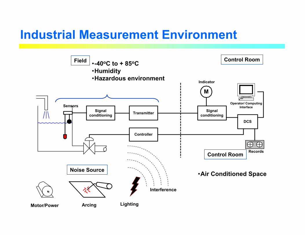
Industrial Measurement Environment

Signalconditioning Transmitter

SensorsSignal

conditioning

M

DCS

Operator/ ComputingInterface

Controller

Records

Indicator

Motor/Power Arcing Lighting

Noise Source

Field Control Room

Control Room

•-40oC to + 85oC•Humidity•Hazardous environment

Interference

•Air Conditioned Space

Objectives

• Able to read and interpret the manufacturer’s specifications

• Understand the physical principles of various sensors

• Able to design a simple measurement system from specifications:

– Selection of Sensors– Design signal conditioners and transmitters

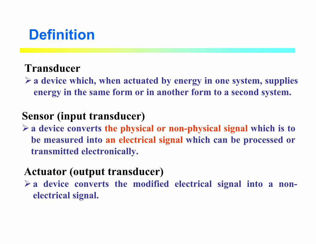
Definition

Transducera device which, when actuated by energy in one system, supplies energy in the same form or in another form to a second system.

Sensor (input transducer)a device converts the physical or non-physical signal which is to be measured into an electrical signal which can be processed or transmitted electronically.

Actuator (output transducer)a device converts the modified electrical signal into a non-electrical signal.

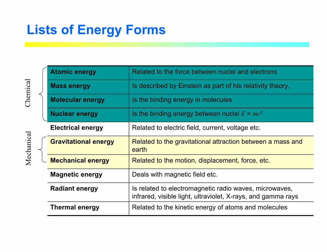
Related to the motion, displacement, force, etc.Mechanical energy

Is the binding energy in moleculesMolecular energy

Is the binding energy between nuclei E = mc2Nuclear energy

Is described by Einstein as part of his relativity theory, Mass energy

Related to the kinetic energy of atoms and moleculesThermal energy

Is related to electromagnetic radio waves, microwaves, infrared, visible light, ultraviolet, X-rays, and gamma rays

Radiant energy

Deals with magnetic field etc.Magnetic energy

Related to the gravitational attraction between a mass and earth

Gravitational energy

Related to electric field, current, voltage etc.Electrical energy

Related to the force between nuclei and electronsAtomic energy

Lists of Energy FormsM

echa

nica

lC

hem

ical

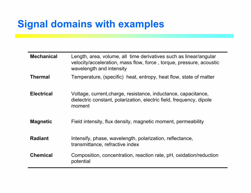
Composition, concentration, reaction rate, pH, oxidation/reduction potential

Chemical

Intensify, phase, wavelength, polarization, reflectance, transmittance, refractive index

Radiant

Field intensity, flux density, magnetic moment, permeabilityMagnetic

Voltage, current,charge, resistance, inductance, capacitance, dielectric constant, polarization, electric field, frequency, dipole moment

Electrical

Temperature, (specific) heat, entropy, heat flow, state of matterThermal

Length, area, volume, all time derivatives such as linear/angular velocity/acceleration, mass flow, force , torque, pressure, acoustic wavelength and intensity

Mechanical

Signal domains with examples

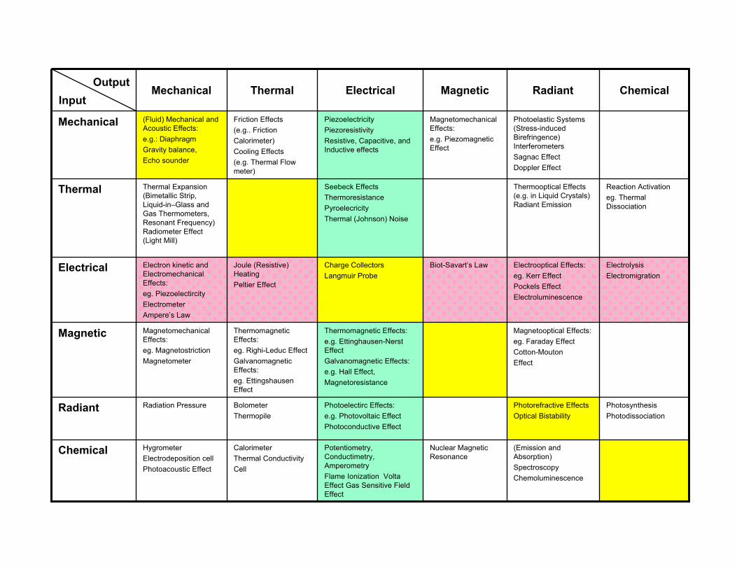
(Emission and Absorption)Spectroscopy Chemoluminescence

Nuclear Magnetic Resonance

Potentiometry, Conductimetry, AmperometryFlame Ionization Volta Effect Gas Sensitive Field Effect

CalorimeterThermal ConductivityCell

HygrometerElectrodeposition cellPhotoacoustic Effect

Chemical

PhotosynthesisPhotodissociation

Photorefractive EffectsOptical Bistability

Photoelectirc Effects:e.g. Photovoltaic EffectPhotoconductive Effect

BolometerThermopile

Radiation PressureRadiant

Magnetooptical Effects:eg. Faraday EffectCotton-MoutonEffect

Thermomagnetic Effects:e.g. Ettinghausen-NerstEffectGalvanomagnetic Effects:e.g. Hall Effect, Magnetoresistance

ThermomagneticEffects:eg. Righi-Leduc EffectGalvanomagneticEffects:eg. EttingshausenEffect

MagnetomechanicalEffects:eg. MagnetostrictionMagnetometer

Magnetic

ElectrolysisElectromigration

Electrooptical Effects:eg. Kerr EffectPockels EffectElectroluminescence

Biot-Savart’s LawCharge CollectorsLangmuir Probe

Joule (Resistive) HeatingPeltier Effect

Electron kinetic and Electromechanical Effects:eg. PiezoelectircityElectrometerAmpere’s Law

Electrical

Reaction Activation eg. Thermal Dissociation

Thermooptical Effects (e.g. in Liquid Crystals) Radiant Emission

Seebeck EffectsThermoresistancePyroelecricityThermal (Johnson) Noise

Thermal Expansion (Bimetallic Strip, Liquid-in–Glass and Gas Thermometers, Resonant Frequency) Radiometer Effect (Light Mill)

Thermal

Photoelastic Systems (Stress-induced Birefringence) Interferometers Sagnac Effect Doppler Effect

MagnetomechanicalEffects:e.g. PiezomagneticEffect

PiezoelectricityPiezoresistivityResistive, Capacitive, and Inductive effects

Friction Effects(e.g.. FrictionCalorimeter)Cooling Effects(e.g. Thermal Flow meter)

(Fluid) Mechanical and Acoustic Effects: e.g.: DiaphragmGravity balance,Echo sounder

Mechanical

ChemicalRadiantMagneticElectricalThermalMechanicalInput

Output

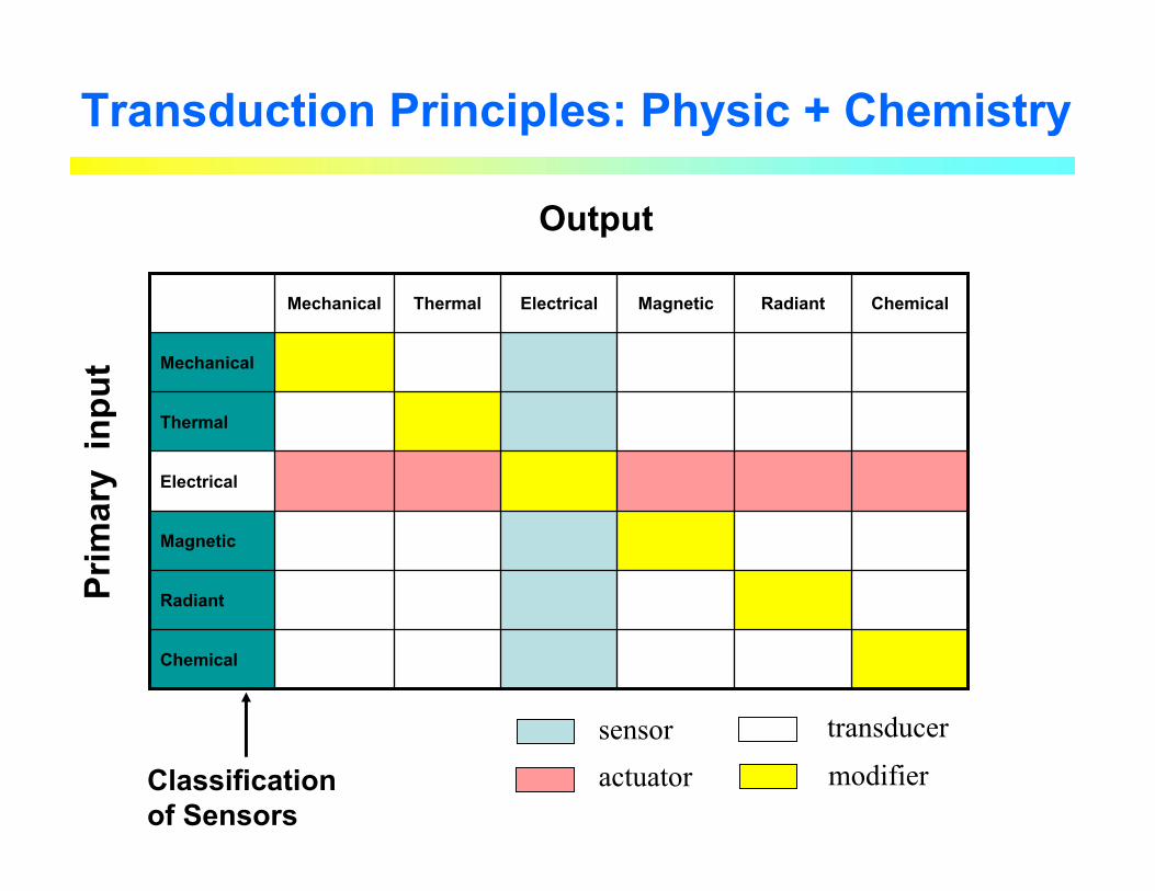
Transduction Principles: Physic + Chemistry

Chemical

Radiant

Magnetic

Electrical

Thermal

Mechanical

ChemicalRadiantMagneticElectricalThermalMechanical

Prim

ary

inpu

t

Output

Classification of Sensors

sensoractuator modifier

transducer

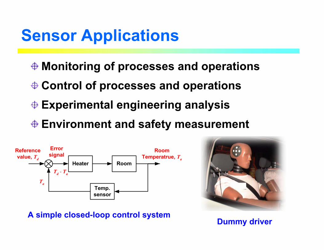
Sensor Applications

Monitoring of processes and operationsControl of processes and operationsExperimental engineering analysisEnvironment and safety measurement

A simple closed-loop control system

Heater Room

Temp.sensor

Errorsignal

Referencevalue, Td

Ta

Td - Ta

RoomTemperatrue, Ta

Dummy driver

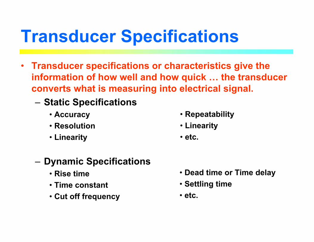
Transducer Specifications• Transducer specifications or characteristics give the

information of how well and how quick … the transducer converts what is measuring into electrical signal.– Static Specifications

• Accuracy• Resolution • Linearity

– Dynamic Specifications• Rise time• Time constant• Cut off frequency

• Repeatability• Linearity• etc.

• Dead time or Time delay• Settling time• etc.

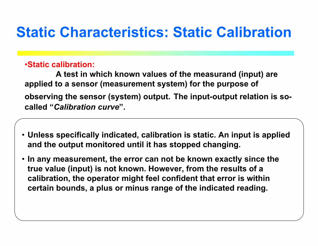
Static Characteristics: Static Calibration

•Static calibration:A test in which known values of the measurand (input) are

applied to a sensor (measurement system) for the purpose of observing the sensor (system) output. The input-output relation is so-called “Calibration curve”.

• Unless specifically indicated, calibration is static. An input is applied and the output monitored until it has stopped changing.

• In any measurement, the error can not be known exactly since thetrue value (input) is not known. However, from the results of a calibration, the operator might feel confident that error is within certain bounds, a plus or minus range of the indicated reading.

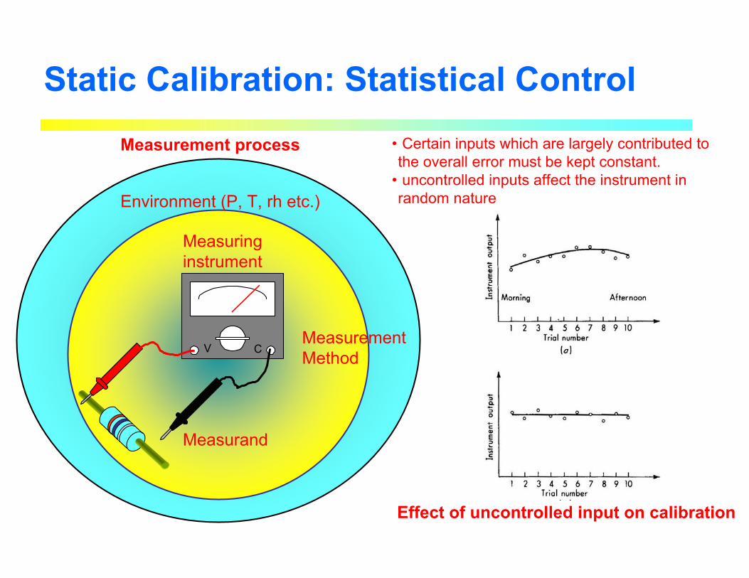
Static Calibration: Statistical Control

V C

Measurand

Measuring instrument

Measurement process

Environment (P, T, rh etc.)

Measurement Method

Effect of uncontrolled input on calibration

• Certain inputs which are largely contributed to the overall error must be kept constant.

• uncontrolled inputs affect the instrument in random nature

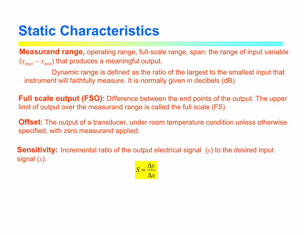
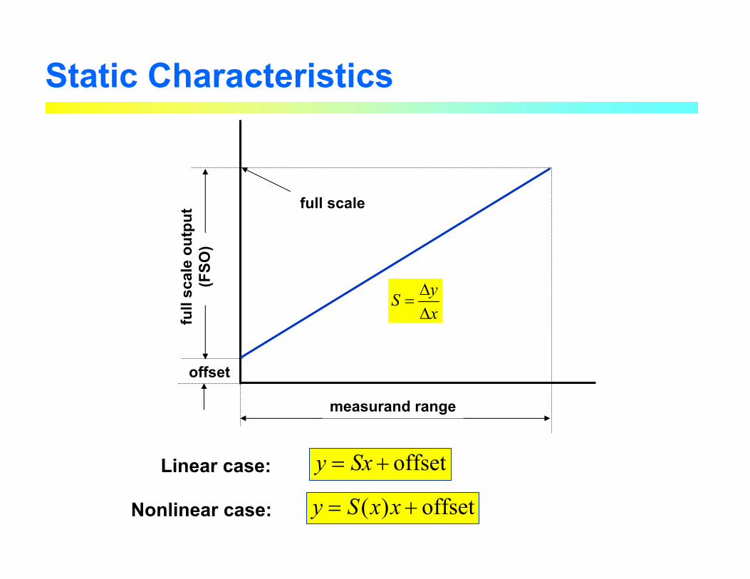
Measurand range, operating range, full-scale range, span: the range of input variable (xmax – xmin) that produces a meaningful output.

Full scale output (FSO): Difference between the end points of the output. The upper limit of output over the measurand range is called the full scale (FS)

Offset: The output of a transducer, under room temperature condition unless otherwise specified, with zero measurand applied.

Static Characteristics

Dynamic range is defined as the ratio of the largest to the smallest input that instrument will faithfully measure. It is normally given in decibels (dB).

Sensitivity: Incremental ratio of the output electrical signal (y) to the desired input signal (x).

ySx

∆=∆

full

scal

e ou

tput

(FSO

)

measurand range

full scale

offset

Static Characteristics

ySx

∆=∆

offset+= SxyLinear case:

Nonlinear case: offset)( += xxSy

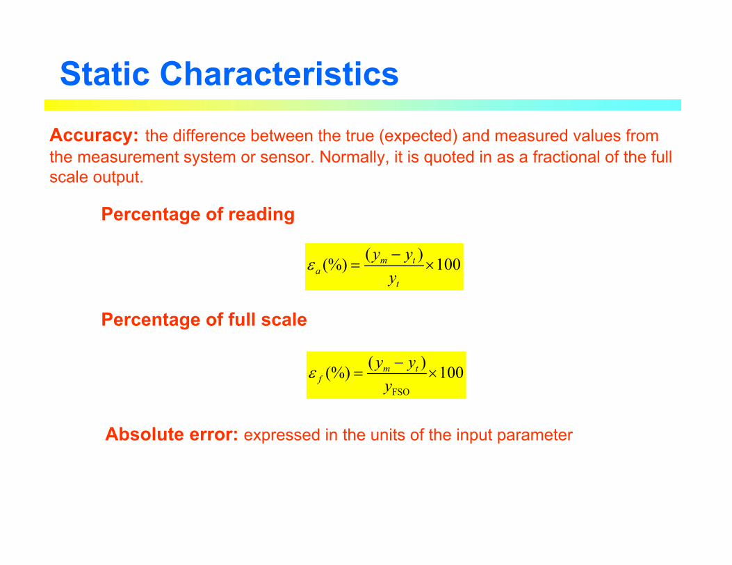
Static CharacteristicsAccuracy: the difference between the true (expected) and measured values from the measurement system or sensor. Normally, it is quoted in as a fractional of the full scale output.

( )(%) 100m ta

t

y yy

ε −= ×

FSO

( )(%) 100m tf

y yy

ε −= ×

Percentage of reading

Percentage of full scale

Absolute error: expressed in the units of the input parameter

Static CharacteristicsResolution: the smallest increment in the value of the measurand that results in a detectable increment in the output. It is expressed in the percentage of the measurand range

max min

Resolution (%) 100xx x

∆= ×

−

If the input is increased from zero, there will be some minimum value below which no output change can be detected, This minimum value defines the Thresholdof the instrument.

Simple optical encoder

Each time the shaft rotates ¼ of a revolution, a pulse will be generated. So, this encoder has a 90oC resolution.

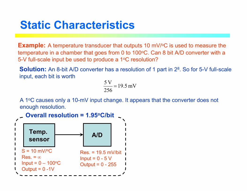
Static CharacteristicsExample: A temperature transducer that outputs 10 mV/oC is used to measure the temperature in a chamber that goes from 0 to 100oC. Can 8 bit A/D converter with a 5-V full-scale input be used to produce a 1oC resolution?

Solution: An 8-bit A/D converter has a resolution of 1 part in 28. So for 5-V full-scale input, each bit is worth

mV 5.19256

V 5=

A 1oC causes only a 10-mV input change. It appears that the converter does not enough resolution.

A/DTemp. sensor

S = 10 mV/oCRes. = ∞Input = 0 – 100oCOutput = 0 -1V

Res. = 19.5 mV/bitInput = 0 - 5 VOutput = 0 - 255

Overall resolution = 1.95oC/bit

Static Characteristics

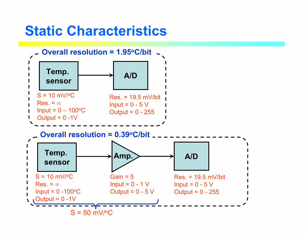
A/DTemp. sensor

S = 10 mV/oCRes. = ∞Input = 0 – 100oCOutput = 0 -1V

Res. = 19.5 mV/bitInput = 0 - 5 VOutput = 0 - 255

Overall resolution = 1.95oC/bit

A/DTemp. sensor

S = 10 mV/oCRes. = ∞Input = 0 -100oCOutput = 0 -1V

Res. = 19.5 mV/bitInput = 0 - 5 VOutput = 0 - 255

Overall resolution = 0.39oC/bit

Gain = 5Input = 0 - 1 VOutput = 0 - 5 V

Amp.

S = 50 mV/oC

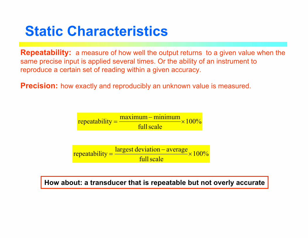
Static CharacteristicsRepeatability: a measure of how well the output returns to a given value when the same precise input is applied several times. Or the ability of an instrument to reproduce a certain set of reading within a given accuracy.

Precision: how exactly and reproducibly an unknown value is measured.

How about: a transducer that is repeatable but not overly accurate

%100scale full

minimummaximumityrepeatabil ×−

=

%100scale full

averagedeviationlargest ityrepeatabil ×−

=

Static Characteristics

Load cell output (mV)

Trail no.

A B

C

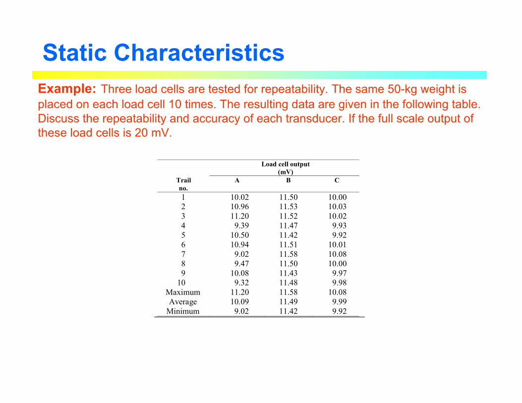
1 10.02 11.50 10.00 2 10.96 11.53 10.03 3 11.20 11.52 10.02 4 9.39 11.47 9.93 5 10.50 11.42 9.92 6 10.94 11.51 10.01 7 9.02 11.58 10.08 8 9.47 11.50 10.00 9 10.08 11.43 9.97

10 9.32 11.48 9.98 Maximum 11.20 11.58 10.08 Average 10.09 11.49 9.99

Minimum 9.02 11.42 9.92

Example: Three load cells are tested for repeatability. The same 50-kg weight is placed on each load cell 10 times. The resulting data are given in the following table. Discuss the repeatability and accuracy of each transducer. If the full scale output of these load cells is 20 mV.

Trial no.

0 1 2 3 4 5 6 7 8 9 10

Out

put (

mV)

9.09.29.49.69.8

10.010.210.410.610.811.011.211.411.6

x

xx

x

x

x

x

x

x

x

Trial no.

0 1 2 3 4 5 6 7 8 9 10

Out

put (

mV)

9.09.29.49.69.8

10.010.210.410.610.811.011.211.411.6

x x x x x x x x x x

Trial no.

0 1 2 3 4 5 6 7 8 9 10

Out

put (

mV)

9.09.29.49.69.8

10.010.210.410.610.811.011.211.411.6

x x x x x x x x x x

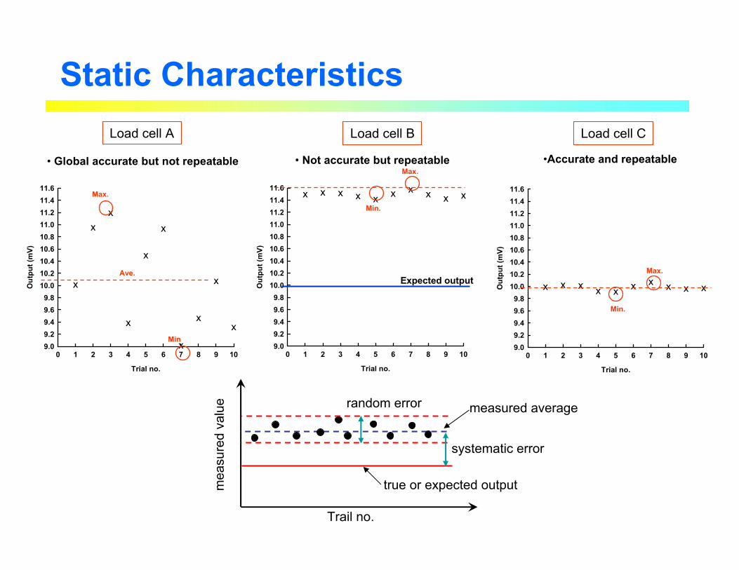
Static CharacteristicsLoad cell A Load cell B Load cell C

Max.

Min

Ave.

Max.

Min.

Max.

Min.

• Global accurate but not repeatable • Not accurate but repeatable •Accurate and repeatable

systematic error

random error

true or expected output

measured average

mea

sure

d va

lue

Trail no.

Expected output

Static Characteristics

Hysteresis: Difference in the output of the sensors for a given input value x, when x is increased and decreased or vice versa. (expressed in % of FSO) (indication of reproducibility)

outp

ut (%

FSO

)

measurand (% range)

0 1000

100 maximumhysteresis

Static Characteristics

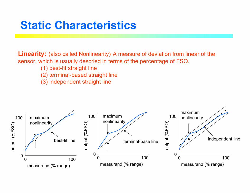
Linearity: (also called Nonlinearity) A measure of deviation from linear of the sensor, which is usually descried in terms of the percentage of FSO.

(1) best-fit straight line (2) terminal-based straight line(3) independent straight line

outp

ut (%

FSO

)

measurand (% range)0 100

0

100 maximumnonlinearity

terminal-base line

outp

ut (%

FSO

)

measurand (% range)0 100

0

100 maximumnonlinearity

best-fit line

outp

ut (%

FSO

)measurand (% range)

0 1000

100maximumnonlinearity

independent line

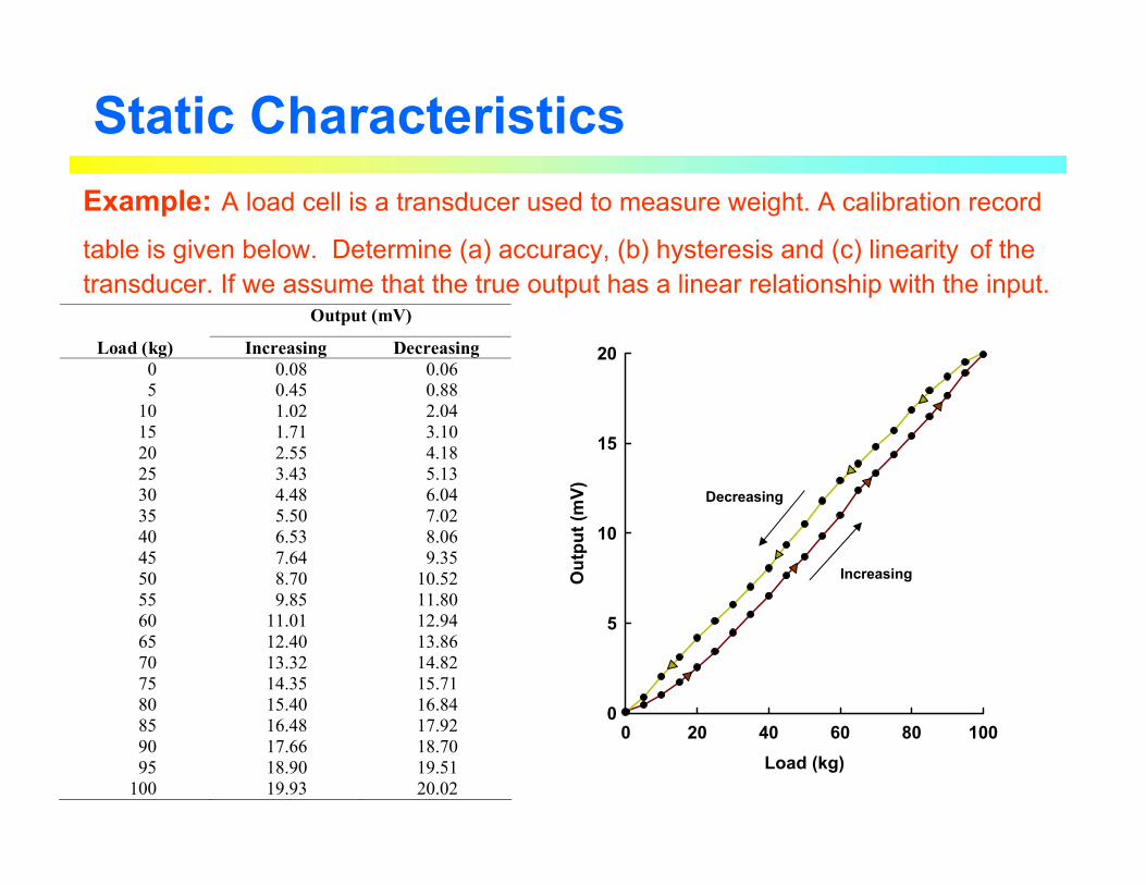
Static CharacteristicsExample: A load cell is a transducer used to measure weight. A calibration record

table is given below. Determine (a) accuracy, (b) hysteresis and (c) linearity of the transducer. If we assume that the true output has a linear relationship with the input.

Output (mV)

Load (kg) Increasing Decreasing 0 0.08 0.06 5 0.45 0.88

10 1.02 2.04 15 1.71 3.10 20 2.55 4.18 25 3.43 5.13 30 4.48 6.04 35 5.50 7.02 40 6.53 8.06 45 7.64 9.35 50 8.70 10.52 55 9.85 11.80 60 11.01 12.94 65 12.40 13.86 70 13.32 14.82 75 14.35 15.71 80 15.40 16.84 85 16.48 17.92 90 17.66 18.70 95 18.90 19.51

100 19.93 20.02

Load (kg)0 20 40 60 80 100

Out

put (

mV)

0

5

10

15

20

Increasing

Decreasing

25 5 5.13 -0.13 -0.65 -2.6020 4 4.18 -0.18 -0.90 -4.5015 3 3.10 -0.10 -0.50 -3.3310 2 2.04 -0.04 -0.20 -2.00

5 1 0.88 0.12 0.60 12.000 0 0.06 -0.06 -0.30 a Load (kg)

0 20 40 60 80 100O

utpu

t (m

V)0

5

10

15

20

Increasing

Decreasing

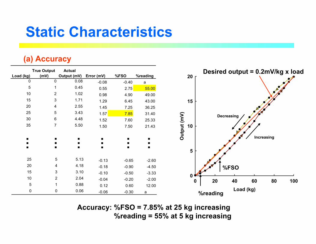
Static Characteristics(a) Accuracy

Load (kg)True Output

(mV)Actual

Output (mV) Error (mV) %FSO %reading0 0 0.08 -0.08 -0.40 a5 1 0.45 0.55 2.75 55.00

10 2 1.02 0.98 4.90 49.0015 3 1.71 1.29 6.45 43.0020 4 2.55 1.45 7.25 36.2525 5 3.43 1.57 7.85 31.4030 6 4.48 1.52 7.60 25.3335 7 5.50 1.50 7.50 21.43

… … … … … …%FSO

%reading

Desired output = 0.2mV/kg x load

Accuracy: %FSO = 7.85% at 25 kg increasing%reading = 55% at 5 kg increasing

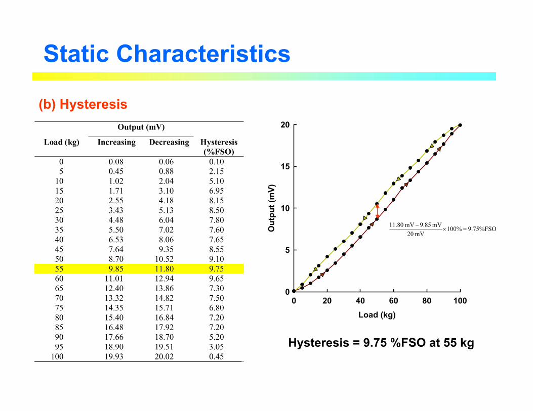
Static Characteristics

(b) Hysteresis

Load (kg)0 20 40 60 80 100

Out

put (

mV)

0

5

10

15

20 Output (mV)

Load (kg) Increasing Decreasing

Hysteresis (%FSO)

0 0.08 0.06 0.10 5 0.45 0.88 2.15

10 1.02 2.04 5.10 15 1.71 3.10 6.95 20 2.55 4.18 8.15 25 3.43 5.13 8.50 30 4.48 6.04 7.80 35 5.50 7.02 7.60 40 6.53 8.06 7.65 45 7.64 9.35 8.55 50 8.70 10.52 9.10 55 9.85 11.80 9.75 60 11.01 12.94 9.65 65 12.40 13.86 7.30 70 13.32 14.82 7.50 75 14.35 15.71 6.80 80 15.40 16.84 7.20 85 16.48 17.92 7.20 90 17.66 18.70 5.20 95 18.90 19.51 3.05

100 19.93 20.02 0.45

%FSO75.9%100mV20

mV 9.85mV 11.80=×

−

Hysteresis = 9.75 %FSO at 55 kg

Load (kg)0 20 40 60 80 100

Out

put (

mV)

0

5

10

15

20

endpoint

%FSO85.7%100mV20

mV 43.3mV 00.5=×

−

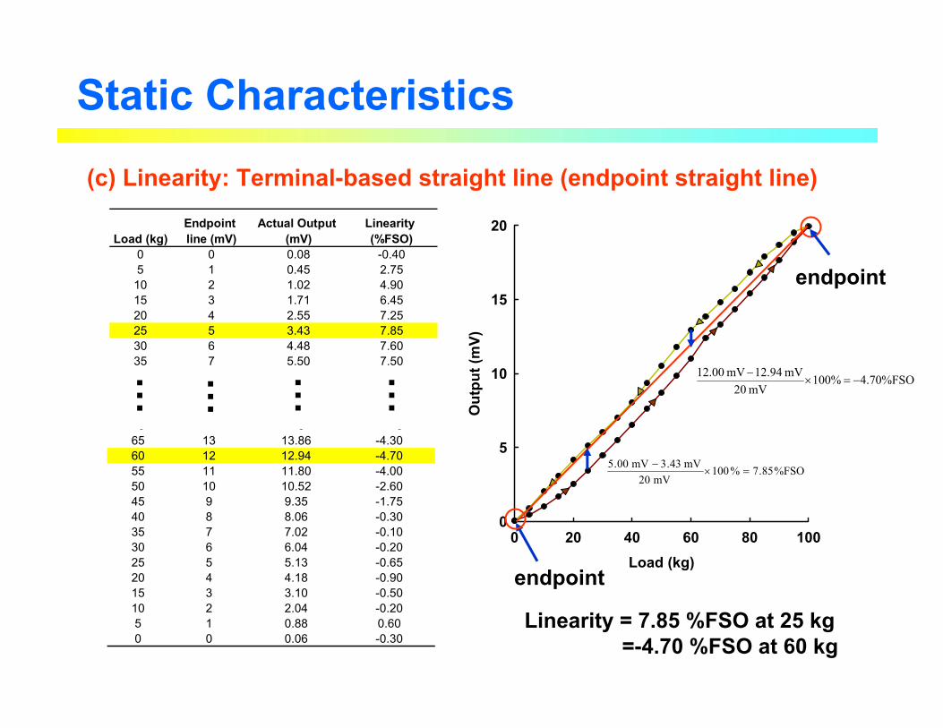
Static Characteristics

(c) Linearity: Terminal-based straight line (endpoint straight line)

endpoint

Load (kg)Endpoint line (mV)

Actual Output (mV)

Linearity (%FSO)

0 0 0.08 -0.405 1 0.45 2.7510 2 1.02 4.9015 3 1.71 6.4520 4 2.55 7.2525 5 3.43 7.8530 6 4.48 7.6035 7 5.50 7.5040 8 6 3 3

0 8 065 13 13.86 -4.3060 12 12.94 -4.7055 11 11.80 -4.0050 10 10.52 -2.6045 9 9.35 -1.7540 8 8.06 -0.3035 7 7.02 -0.1030 6 6.04 -0.2025 5 5.13 -0.6520 4 4.18 -0.9015 3 3.10 -0.5010 2 2.04 -0.205 1 0.88 0.600 0 0.06 -0.30

… … … …

Linearity = 7.85 %FSO at 25 kg=-4.70 %FSO at 60 kg

%FSO70.4%100mV 20

mV 94.12mV 00.21−=×

−

Load (kg)0 20 40 60 80 100

Out

put (

mV)

0

5

10

15

20

%FSO85.5%100mV20

mV 48.4mV 65.5=×

−

Static Characteristics

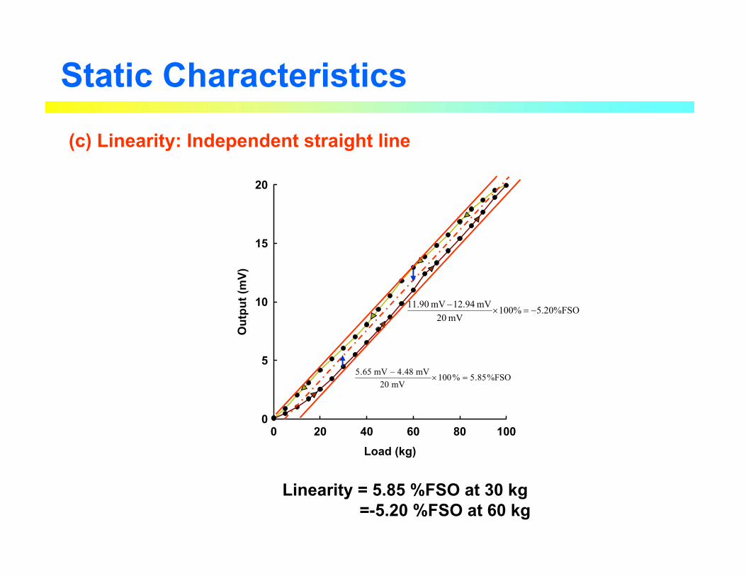
(c) Linearity: Independent straight line

Linearity = 5.85 %FSO at 30 kg=-5.20 %FSO at 60 kg

%FSO20.5%100mV 20

mV 94.12mV 90.11−=×

−

Static Characteristics

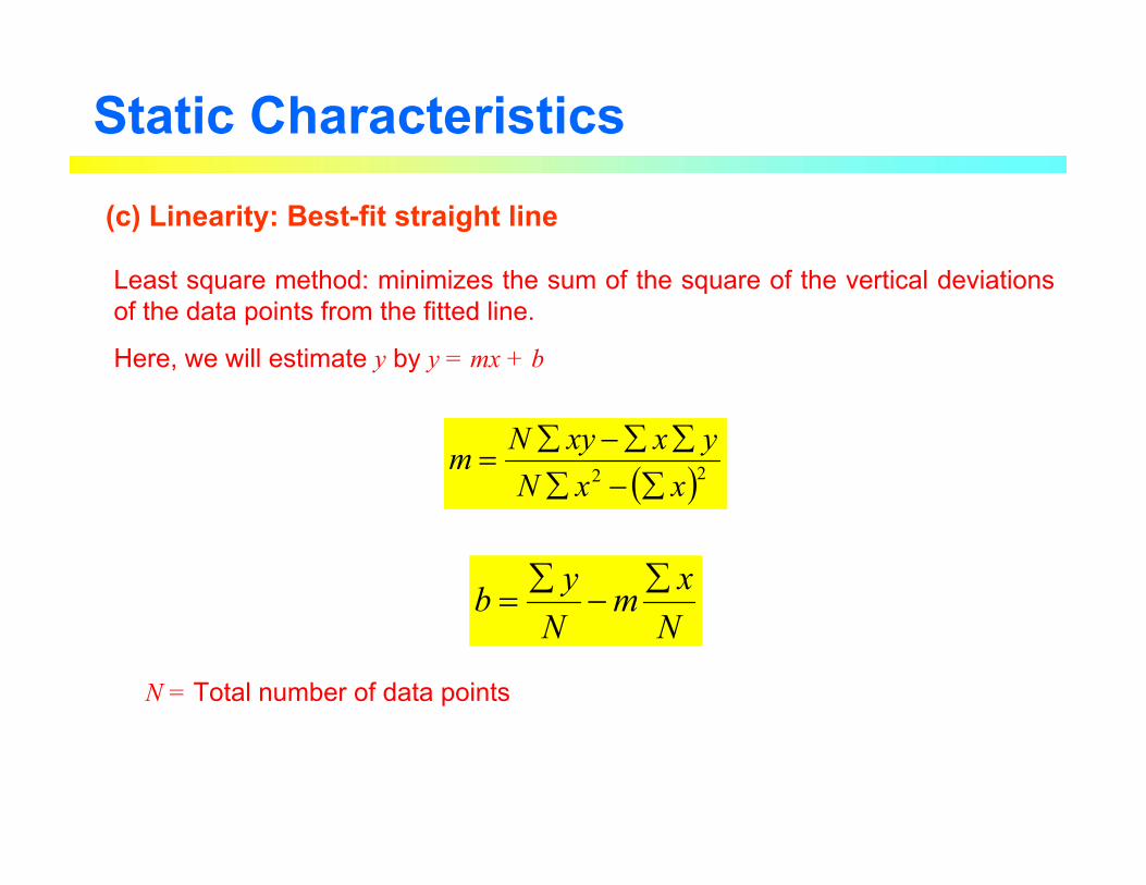
(c) Linearity: Best-fit straight line

Least square method: minimizes the sum of the square of the vertical deviations of the data points from the fitted line.

Here, we will estimate y by y = mx + b

N = Total number of data points

( )22 xxNyxxyNm

∑−∑∑∑−∑

=

Nxm

Nyb ∑−

∑=

Static Characteristics

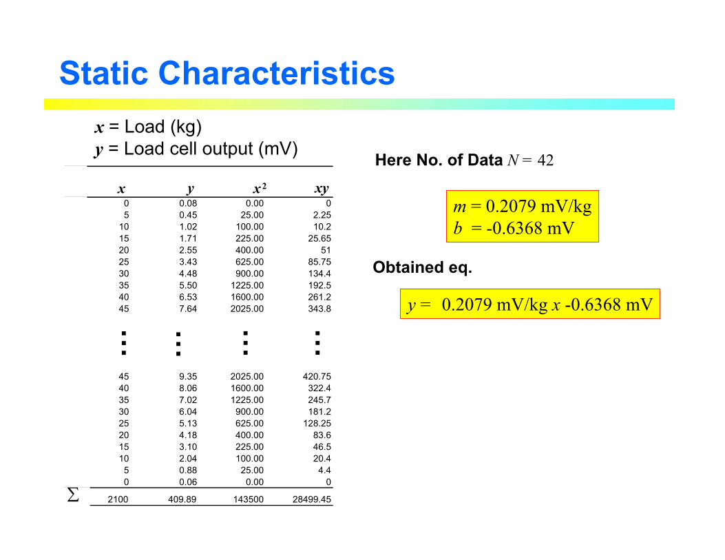
45 9.35 2025.00 420.7540 8.06 1600.00 322.435 7.02 1225.00 245.730 6.04 900.00 181.225 5.13 625.00 128.2520 4.18 400.00 83.615 3.10 225.00 46.510 2.04 100.00 20.4

5 0.88 25.00 4.40 0.06 0.00 0

2100 409.89 143500 28499.45

x = Load (kg)y = Load cell output (mV)

x y x xy0 0.08 0.00 05 0.45 25.00 2.25

10 1.02 100.00 10.215 1.71 225.00 25.6520 2.55 400.00 5125 3.43 625.00 85.7530 4.48 900.00 134.435 5.50 1225.00 192.540 6.53 1600.00 261.245 7.64 2025.00 343.8

2

… … … …

∑

Here No. of Data N = 42

m = 0.2079 mV/kgb = -0.6368 mV

y = 0.2079 mV/kg x -0.6368 mV

Obtained eq.

Load (kg)0 20 40 60 80 100

Out

put (

mV)

0

5

10

15

20

%FSO70.5%100mV20.15

mV 86.7mV .536=×

−

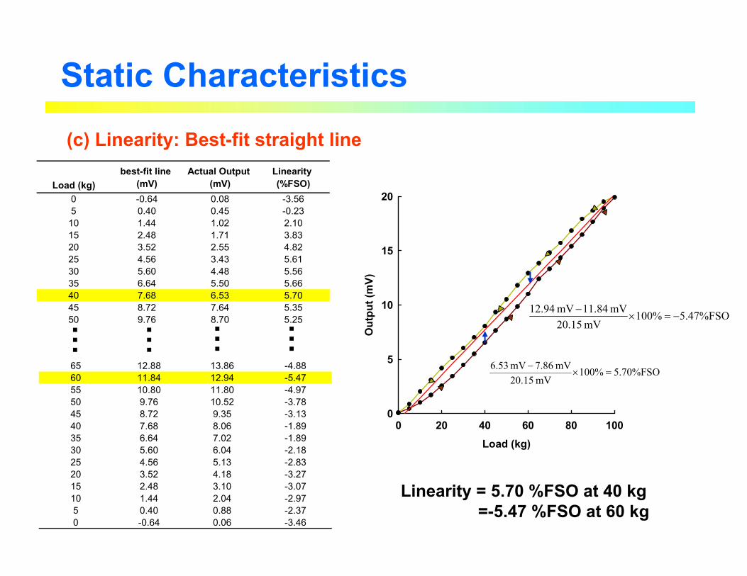
Static Characteristics

(c) Linearity: Best-fit straight line

… … … …Linearity = 5.70 %FSO at 40 kg

=-5.47 %FSO at 60 kg

%FSO47.5%100mV20.15

mV 84.11mV 2.941−=×

−

Load (kg)best-fit line

(mV)Actual Output

(mV)Linearity (%FSO)

0 -0.64 0.08 -3.565 0.40 0.45 -0.2310 1.44 1.02 2.1015 2.48 1.71 3.8320 3.52 2.55 4.8225 4.56 3.43 5.6130 5.60 4.48 5.5635 6.64 5.50 5.6640 7.68 6.53 5.7045 8.72 7.64 5.3550 9.76 8.70 5.2555 10 80 9 85 4 70

0 3 9 8 965 12.88 13.86 -4.8860 11.84 12.94 -5.4755 10.80 11.80 -4.9750 9.76 10.52 -3.7845 8.72 9.35 -3.1340 7.68 8.06 -1.8935 6.64 7.02 -1.8930 5.60 6.04 -2.1825 4.56 5.13 -2.8320 3.52 4.18 -3.2715 2.48 3.10 -3.0710 1.44 2.04 -2.975 0.40 0.88 -2.370 -0.64 0.06 -3.46

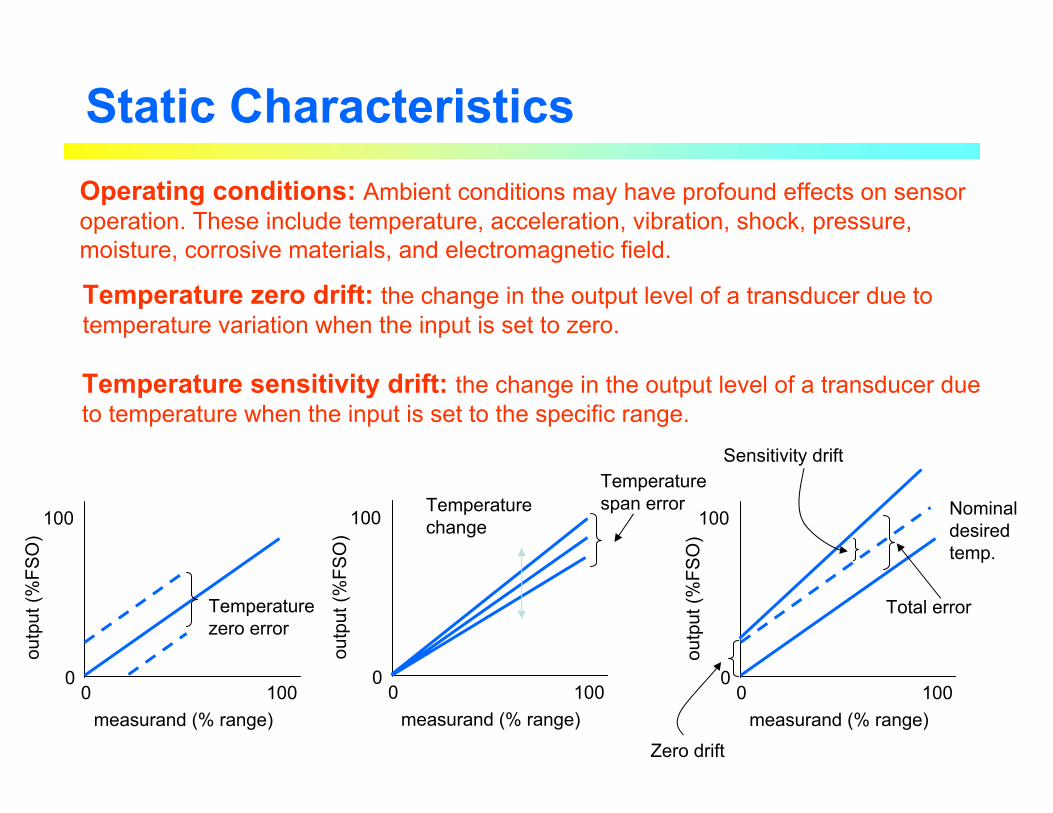
Static CharacteristicsOperating conditions: Ambient conditions may have profound effects on sensor operation. These include temperature, acceleration, vibration, shock, pressure, moisture, corrosive materials, and electromagnetic field.

outp

ut (%

FSO

)

measurand (% range)0 100

0

100

Temperature span errorTemperature

change

outp

ut (%

FSO

)

measurand (% range)0 100

0

100

Temperature zero error

outp

ut (%

FSO

)measurand (% range)

0 1000

100

Zero drift

Sensitivity drift

Total error

Nominal desired temp.

Temperature zero drift: the change in the output level of a transducer due to temperature variation when the input is set to zero.

Temperature sensitivity drift: the change in the output level of a transducer due to temperature when the input is set to the specific range.

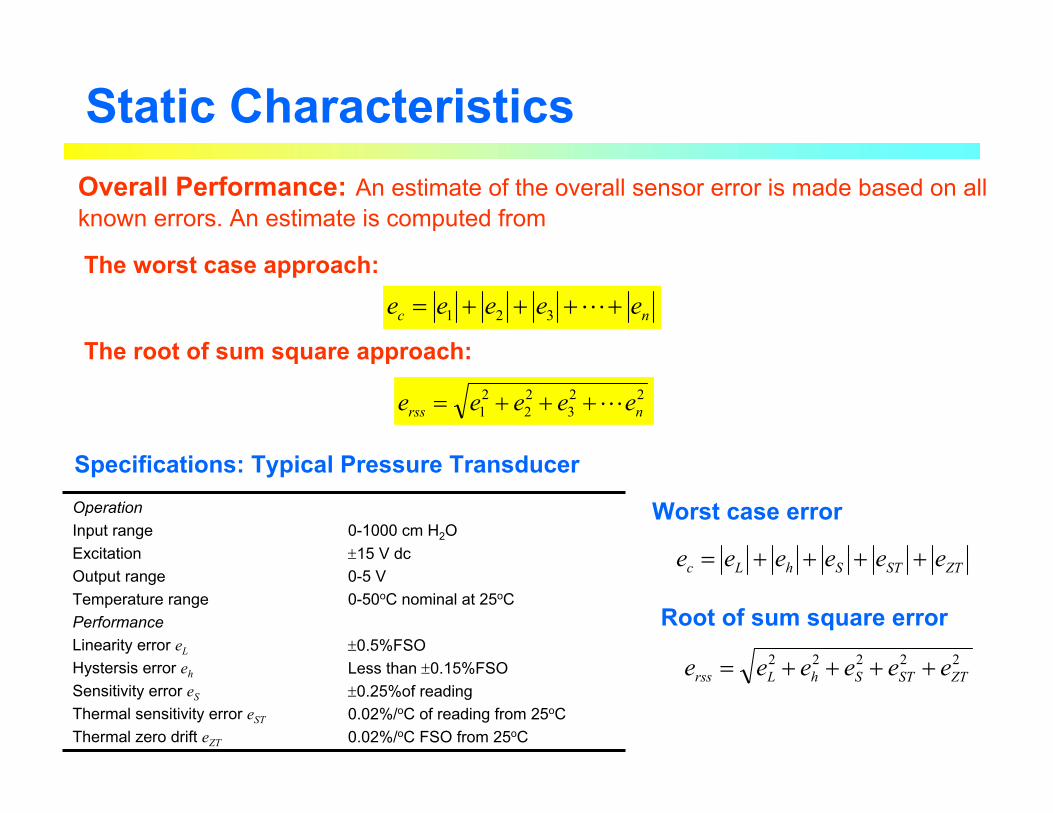
Overall Performance: An estimate of the overall sensor error is made based on all known errors. An estimate is computed from

Static Characteristics

The worst case approach:

The root of sum square approach:nc eeeee ++++= L321

223

22

21 nrss eeeee L+++=

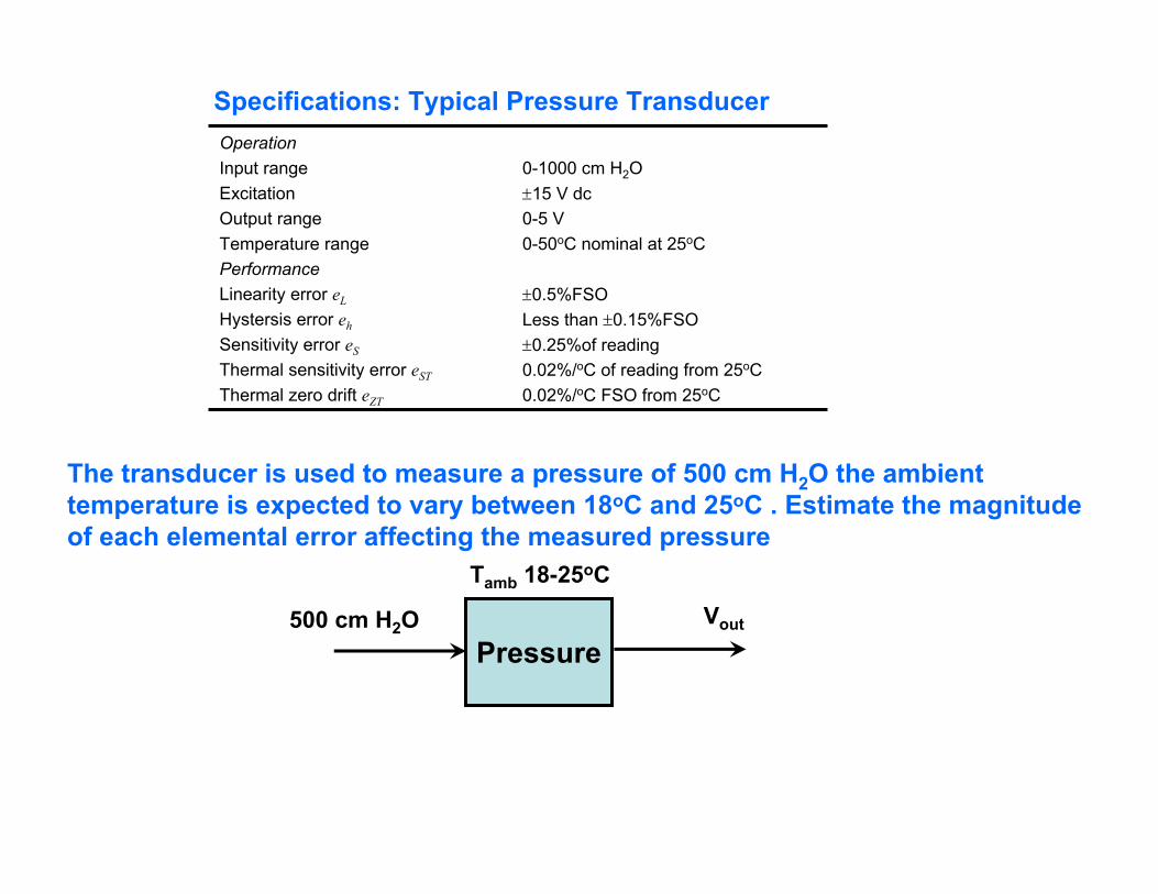
0-1000 cm H2O±15 V dc0-5 V0-50oC nominal at 25oC

±0.5%FSOLess than ±0.15%FSO±0.25%of reading0.02%/oC of reading from 25oC0.02%/oC FSO from 25oC

OperationInput rangeExcitationOutput rangeTemperature rangePerformanceLinearity error eL

Hystersis error eh

Sensitivity error eS

Thermal sensitivity error eST

Thermal zero drift eZT

Specifications: Typical Pressure Transducer

22222ZTSTShLrss eeeeee ++++=

ZTSTShLc eeeeee ++++=

Worst case error

Root of sum square error

0-1000 cm H2O±15 V dc0-5 V0-50oC nominal at 25oC

±0.5%FSOLess than ±0.15%FSO±0.25%of reading0.02%/oC of reading from 25oC0.02%/oC FSO from 25oC

OperationInput rangeExcitationOutput rangeTemperature rangePerformanceLinearity error eL

Hystersis error eh

Sensitivity error eS

Thermal sensitivity error eST

Thermal zero drift eZT

Specifications: Typical Pressure Transducer

The transducer is used to measure a pressure of 500 cm H2O the ambient temperature is expected to vary between 18oC and 25oC . Estimate the magnitude of each elemental error affecting the measured pressure

Pressure500 cm H2O

Tamb 18-25oC

Vout

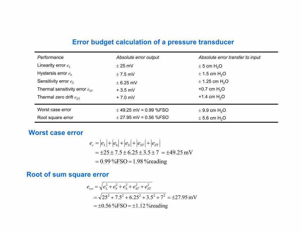
± 9.9 cm H2O

± 5.6 cm H2O

± 49.25 mV = 0.99 %FSO ± 27.95 mV = 0.56 %FSO

Worst case error

Root square error

Absolute error output

± 25 mV

± 7.5 mV

± 6.25 mV+ 3.5 mV+ 7.0 mV

Absolute error transfer to input

± 5 cm H2O

± 1.5 cm H2O

± 1.25 cm H2O

+0.7 cm H2O

+1.4 cm H2O

Performance

Linearity error eL

Hystersis error eh

Sensitivity error eS

Thermal sensitivity error eST

Thermal zero drift eZT

Error budget calculation of a pressure transducer

%reading 1.98 %FSO 0.99 mV 25.49 7 5.3 25.6 5.7 25

==±=±±±±±=

++++= ZTSTShLc eeeeee

%reading 1.12 %FSO 0.56 mV 95.2775.325.65.725 22222

22222

±=±=±=++++=

++++= ZTSTShLrss eeeeee

Worst case error

Root of sum square error

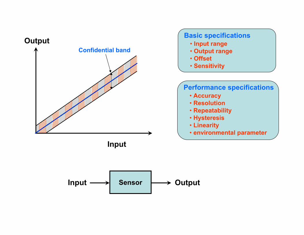
Performance specifications• Accuracy• Resolution• Repeatability• Hysteresis• Linearity• environmental parameter

Confidential bandOutput

Input

Basic specifications• Input range• Output range• Offset• Sensitivity

SensorInput Output