© 2015 Lakshmi Gururaja Rao

DESIGN AND OPTIMIZATION OF COMPUTATIONALLY EXPENSIVEENGINEERING SYSTEMS

BY

LAKSHMI GURURAJA RAO

THESIS

Submitted in partial fulfillment of the requirementsfor the degree of Master of Science in Industrial Engineering

in the Graduate College of theUniversity of Illinois at Urbana-Champaign, 2015

Urbana, Illinois

Adviser:

Assistant Professor James T. Allison

Abstract

Engineering systems form the basis on which our day-to-day lives depend

on. In many cases, designers are interested in identifying an optimal design

of an engineering system. However, very often, the process of engineering

design optimization is complex and involves time-expensive simulations or

the need to satisfy not just one, but multiple objectives. This thesis aims to

explore the area of efficient optimization algorithms applied to engineering

system design. In particular, the engineering systems discussed here involve

the use of rheologically complex materials. Engineers face many modeling

challenges while trying to design systems with rheological materials, pertain-

ing to mathematical modeling and optimization. However, the use of more

flexible design methods in conjunction with rheologically complex materials

enhances design freedom and diffuses design fixation. The first part of the

thesis discusses the characteristics of such materials and introduces their us-

age in engineering design. A second kind of complex systems include the

ones characterized by multiple objectives and time-expensive simulations.

Design optimization is a cumbersome process in such a case. Using an ap-

proximation or a surrogate model of this kind of system helps to mitigate

computational costs. The use of an adaptive surrogate modeling alogrithm

(along with optimization) is demonstrated on such systems, that involve the

use of complex fluids. The unifying theme of the thesis is the application of

efficient optimization algorithms to computationally expensive material de-

sign problems. In this thesis, we introduce the use of direct optimal control

to identify optimal material function targets. The thesis also details a novel

adaptive surrogate modeling algorithm that was developed to solve multi-

objective optimization problems. Both these ideas are demonstrated with

the help of case studies and analytical examples.

ii

To my parents, for their unconditional love and support.

iii

Acknowledgments

First and foremost, I would like to extend my gratitude to Prof. James

T. Allison, for having given me this opportunity to work with him and for

moulding me into the researcher I am today. His unwavering patience, in-

sightful advice and constant support have been valuable to me during my

graduate school experience. I also had the pleasure of working with Prof.

Randy H. Ewoldt, at the Mechanical Science and Engineering department,

UIUC. Both the research projects that are discussed in this thesis were the

result of a collaborative effort with Prof. Ewoldt’s research group. What

seemed to me like a new and (hence) intimidating area of research initially,

was greatly simplified thanks to the numerous interesting discussions with

Prof. Ewoldt.

I wish to thank my fellow graduate students at the Engineering Systems

Design Lab (ESDL) - Anand, Dan, Tinghao, Jeff, Ashish, Jason, Danny and

Adam. I have enjoyed the conversations at 406 TB, that were not always

(almost always not) about research. I have always received help and support

and a wondrous bout of good humor when I have needed it, and I am ex-

tremely grateful for that. I am more than grateful to the ISE department for

supporting me through Teaching Assistantships and I deeply appreciate the

kindness and help I received from Holly Kizer and the other adminstrative

staff, right from the day I started my Master’s program.

I was fortunate to work with Rebecca Corman and Jonathon Schuh from

Prof. Ewoldt’s research group. They made the many hours spent at MEL

more enjoyable and hence, more fruitful. I would like to thank Yong Hoon

Lee for his tireless work in the recent past, with regards to both my research

projects.

My acknowledgement would be incomplete without mentioning Neal Davis,

from the Computational Science and Engineering department for our many

conversations about Python, Julia and theories of science and research. I am

iv

thankful for the TA experience he provided me with, and feel fortunate for

having met an inspirational person such as him, during my graduate school

life. One of the earliest inspirations came from Prof. Andreas Kloeckner at

the Computer Science department, UIUC, when I took his course on Nu-

merical Analysis in Spring 2014. I greatly benefited from the course, his

encouraging words and honest professional advice.

Last but definitely not the least, I would like to thank my family of friends

here at Champaign - my roommate, Aparna, who, aside from being my go-to

graphics guide, has been a tremendous sense of support; Sundar, Sabareesh

and Yashwant, for being a part of some of my best times here and a whole

bunch of others who can make my acknowledgement run into pages. I am

extremely thankful to Preethi and Shridhar (at the Ohio State University)

for having faith in my abilities, even at times when I did not believe in them,

myself. I was lucky to live close to my immediate family at Purdue. I wish

to thank my uncle, for being my role model since the time I was young and

encouraging me to always aim high; my aunt, for being a wonderful host and

my six-year-old cousin, Mukund, for showing me the best kind of affection.

Finally, I would like to thank my parents and my grandparents back home,

who have always been a positive influence and have given me the utmost

freedom and carved out opportunities for me, at every stage of my life.

v

TABLE OF CONTENTS

List of Tables . . . . . . . . . . . . . . . . . . . . . . . . . . . . . . viii

List of Figures . . . . . . . . . . . . . . . . . . . . . . . . . . . . . ix

Nomenclature . . . . . . . . . . . . . . . . . . . . . . . . . . . . . . xi

CHAPTER 1 Introduction . . . . . . . . . . . . . . . . . . . . . . 1

CHAPTER 2 Rheological materials . . . . . . . . . . . . . . . . 42.1 Engineering Design with soft materials . . . . . . . . . . . . . 42.2 Viscoelastic materials . . . . . . . . . . . . . . . . . . . . . . . 5

CHAPTER 3 Design Optimization via material functiontargets . . . . . . . . . . . . . . . . . . . . . . . . . . . . . . . . 143.1 Relaxation Modulus as the target function . . . . . . . . . . . 143.2 Parameterizations of K(t) . . . . . . . . . . . . . . . . . . . . 183.3 Generalized viscoelastic model . . . . . . . . . . . . . . . . . . 213.4 Integro-Differential Equations (IDEs) . . . . . . . . . . . . . . 233.5 Optimal Control methods . . . . . . . . . . . . . . . . . . . . 25

CHAPTER 4 Numerical Studies on a vibration isolator- Part 1 . . . . . . . . . . . . . . . . . . . . . . . . . . . . . . . . 314.1 Case study . . . . . . . . . . . . . . . . . . . . . . . . . . . . . 314.2 Results . . . . . . . . . . . . . . . . . . . . . . . . . . . . . . . 34

CHAPTER 5 Numerical Studies on a vibration isolator- Part 2 . . . . . . . . . . . . . . . . . . . . . . . . . . . . . . . . 435.1 Formulation of the optimal control problem . . . . . . . . . . 435.2 A single shooting approach . . . . . . . . . . . . . . . . . . . . 465.3 Direct Transcription . . . . . . . . . . . . . . . . . . . . . . . 495.4 Results . . . . . . . . . . . . . . . . . . . . . . . . . . . . . . . 505.5 Conclusions . . . . . . . . . . . . . . . . . . . . . . . . . . . . 51

CHAPTER 6 Adaptive Surrogate Modeling based Multi-Objective Optimization . . . . . . . . . . . . . . . . . . . . . . 566.1 Adaptive SM Methodology . . . . . . . . . . . . . . . . . . . . 576.2 ASM-MOO Algorithm Framework . . . . . . . . . . . . . . . . 59

vi

CHAPTER 7 Numerical Studies and Results using Adap-tive Surrogate Modeling . . . . . . . . . . . . . . . . . . . . . 697.1 Analytical Example . . . . . . . . . . . . . . . . . . . . . . . . 697.2 Design for Efficient Fluid Power . . . . . . . . . . . . . . . . . 717.3 Conclusions and Future Work . . . . . . . . . . . . . . . . . . 76

CHAPTER 8 Conclusion . . . . . . . . . . . . . . . . . . . . . . . 77

APPENDIX A High Frequency scaling of displacementamplitude . . . . . . . . . . . . . . . . . . . . . . . . . . . . . . . 78A.1 Initial Case (Spring only) . . . . . . . . . . . . . . . . . . . . . 78A.2 Spring + Linear Dashpot . . . . . . . . . . . . . . . . . . . . . 79A.3 Spring + Generalized Viscoelastic Element . . . . . . . . . . . 79

REFERENCES . . . . . . . . . . . . . . . . . . . . . . . . . . . . . . 85

vii

List of Tables

3.1 Relaxation kernel K(t) for 1-D systems . . . . . . . . . . . . . 15

4.1 Optimization results for the vibration isolator case studybased on existing viscoelastic models . . . . . . . . . . . . . . 36

4.2 Optimization results from the extension of vibration isola-tor case study with existing viscoelastic models and over arange of frequencies . . . . . . . . . . . . . . . . . . . . . . . . 40

5.1 Optimal objective function values from Single Shootingand Direct Transcription . . . . . . . . . . . . . . . . . . . . . 51

7.1 Analytical Problem - Results . . . . . . . . . . . . . . . . . . 717.2 Measured Geometric Parameters. . . . . . . . . . . . . . . . . 727.3 Case Study - Results . . . . . . . . . . . . . . . . . . . . . . . 75

viii

List of Figures

2.1 Product Design Process . . . . . . . . . . . . . . . . . . . . . 52.2 Creep and Stress Relaxation plots . . . . . . . . . . . . . . . . 72.3 Dynamic Loading and Hysteresis . . . . . . . . . . . . . . . . 82.4 Maxwell model for a viscoelastic material. . . . . . . . . . . . 112.5 Kelvin-Voigt model for a viscoelastic material. . . . . . . . . . 12

3.1 Parameterizations of K(t) . . . . . . . . . . . . . . . . . . . . 203.2 A discrete topology can be generalized by the introduction

of a viscoelastic element. . . . . . . . . . . . . . . . . . . . . . 223.3 Convolution example . . . . . . . . . . . . . . . . . . . . . . . 293.4 Convolution of f(t) and g(t) . . . . . . . . . . . . . . . . . . . 30

4.1 Design of optimal viscoelastic vibration isolation for a 1-dimensional spring-mass system . . . . . . . . . . . . . . . . . 31

4.2 Design involving a generalized viscoelastic element withrelaxation kernel K(t) . . . . . . . . . . . . . . . . . . . . . . 35

4.3 Optimized performance and design . . . . . . . . . . . . . . . 384.4 Case Study extension . . . . . . . . . . . . . . . . . . . . . . . 394.5 Results of the case study extension to a range of natural

frequencies . . . . . . . . . . . . . . . . . . . . . . . . . . . . . 41

5.1 Direct Optimal Control applied to the case study . . . . . . . 455.2 Convolution sum validation . . . . . . . . . . . . . . . . . . . 465.3 Unstable Dynamics . . . . . . . . . . . . . . . . . . . . . . . . 485.4 Optimal State trajectories of Single Shooting and Direct

Transcription implementations . . . . . . . . . . . . . . . . . . 525.5 Optimal K(t) trajectories of Single Shooting and Direct

Transcription implementations . . . . . . . . . . . . . . . . . . 53

6.1 Strategies for SM-based design optimization . . . . . . . . . . 586.2 ASM-MOO algorithm . . . . . . . . . . . . . . . . . . . . . . . 606.3 Octree-based sampling algorithm to update the sampling

domain . . . . . . . . . . . . . . . . . . . . . . . . . . . . . . . 676.4 Conceptual illustration of validation point and sample point

generation . . . . . . . . . . . . . . . . . . . . . . . . . . . . . 68

ix

7.1 Analytical Problem - Pareto set . . . . . . . . . . . . . . . . . 707.2 Analytical Problem - Pareto design values . . . . . . . . . . . 707.3 Experimental setup. Design variables are defined in Eqn. (7.2). 727.4 Case Study - Pareto set in design space . . . . . . . . . . . . . 747.5 Case Study - Pareto set . . . . . . . . . . . . . . . . . . . . . 75

x

Nomenclature

φ(·) Boundary constraints in optimal control

ψ Gram matrix of the Radial Basis Functions

ξ Dynamic system state variable vector

Ξ(·) Discretized states in direct transcription

ζ(·) Defect constraints in direct transcription

ε(t) Strain

η, λ Maxwell Parameters

ηa Apparent viscosity of fluid power problem

f(·) Approximate Objective function of MOO

g(·) Approximate Inequality constraint of MOO

h(·) Approximate Equality constraint of MOO

C(·) Path constraints in optimal control

fd State derivative function optimal control

f(·) Objective function of MOO

g(·) Inequality constraint of MOO

h(·) Equality constraint of MOO

I Convolution sum

u Control input in optimal control

xi

w Weights of the Radial Basis Functions

x∗ Optimal design variable

xLB,xUB Lower and upper bounds of design variables of MOO

L(·) Lagrangian cost function in optimal control

M(·) Meyer cost function in optimal control

σ(t) Stress

ω∗ Natural frequency

Ds The sampling domain, from which sampling points are taken

Du Updated sampling domain

D Texture depth of fluid power problem

Dm The modeling domain that forms the basis for the surrogate model

construction

Ds Feasible Sampling Domain

Du Updated feasible sampling domain

Dv Validation domain

F Feasible domain

h Gap height of fluid power problem

hk kth Time step size

k Spring constant

K(t) Relaxation Modulus

K ′′(ω) Dynamic Loss Modulus

K ′(ω) Dynamic Storage Modulus

L Plate length of fluid power problem

m Mass

xii

nt Number of time steps

Sk, n Critical Gel Parameters

T Training Data Set

U Velocity of plate of fluid power problem

W Texture width of fluid power problem

x, x, x Position, Velocity, Acceleration

xiii

CHAPTER 1

Introduction

Engineering systems form the basis on which our day-to-day lives depend

on. Starting from the thermostat that keeps you comfortable in any kind of

temperature to the electrical energy of the satellite orbiting in space, which

helps you watch television at home, engineering systems have found vast

and diverse applications in the real world. The design of such systems is a

challenging task, which involves the understanding of the physics behind the

system as well as the practical viability of the design methodology.

The primary step in engineering design involves modeling the system.

Physical models are constructed, where resources and labor are available.

Computer-based models of engineering systems and simulation of these mod-

els started around the time of World War II [1]. Today, most engineering

systems are modeled with the help of virtual experiments. This serves as a

cost-effective methodology for both designing, testing and making changes to

the existing model and is advantageous in cases where physical modeling is

not feasible. However, there exist many complex engineering systems, whose

virtual modeling is computationally demanding. Despite advances in com-

puting power in the recent past, computationally intensive analysis methods

such as Finite Element Analysis (FEA) and Computational Fluid Dynamics

(CFD) require efficient numerical treatment [2]

In most design problems, engineers are interested in identifying an optimal

design of the system being modeled. The next step in the design process is op-

timization of the engineering system. Computerized models can be optimized

by the use of various optimization algorithms that have been developed [3].

However, when the simulation of the engineering system is time-expensive,

optimization of the system consumes a lot of computing time. For example,

forecasting weather is an expensive computer simulation based on various

atmospheric factors. If we wished to maximize the amount of solar energy

conserved on a given day, we would need to run the simulation multiple

1

times to understand which time of the day recorded the highest range of

temperature, each simulation requiring significant running time. An efficient

optimization technique is essential in order to minimize running time and

computational complexity.

In this thesis, two such optimization routines are presented, which are

applied to engineering systems characterized by time-intensive simulations:

(1) Surrogate modeling, which involves building a data-model of the physical

system and using the data model for the purposes of optimization. (2) Direct

Optimal Control, which is a class of optimal control routines applied to a

dynamic system in order to minimize a cost function associated with it.

The application of these two routines is in the domain of engineering ma-

terial design. Material design is a field with vast applications. Materials are

classified as hard or soft based on their inherent material compliance [4]. In

naıve terms, soft materials are more flexible and exhibit deformation when

subject to a force, as opposed to brittle materials. While designing mate-

rials for engineering systems, engineers have primarily used hard materials.

The complexity of soft materials arises from their unconventional microstruc-

tures. The resulting complexity is carried forward in the modeling of such

materials. Utilizing such materials in engineering design requires specialized

modeling and optimization methods. While complex in nature and model-

ing, the different dynamics of soft materials result in fascinating engineering

applications. The need to use these materials, despite their complexity, thus

stems from the desire to explore the design space, enhance design freedom

and motivate system-level design.

The unifying theme of the thesis is to address the optimization of engi-

neering problems that are time-consuming in their simulation. The thesis

is structured in the following manner. Chapter 2 sets the backdrop of the

application, by further explaining complex materials and the challenges en-

countered in their mathematical modeling. The chapter also discusses the

need to develop efficient numerical methods to model complex materials and

gives a gentle introduction to different methods that are used for the efficient

handling of expensive simulations. It is followed by Chapter 3, which goes

into numerical details and formulation of an efficient optimization technique

utilizing optimal control. This is presented with the help of a case study

involving a vibration attenuation problem in Chapter 4 and 5. The focus is

then shifted to the use of surrogate modeling in Chapter 6. The application

2

of surrogate modeling to alleviate the cost of time-expensive problems is dis-

cussed with a detailed case study in Chapter 7. The results, discussions and

future work are enumerated in Chapter 8.

3

CHAPTER 2

Rheological materials

Rheology pertains to the study of flow of matter, primarily in a liquid state.

It applies to soft solids that respond with a plastic flow rather than elastic

deformation, when subject to an external force [5] . It includes the study of

materials that have a complex microstructure such as muds, sledges, foods

and additives like ketchup, mayonnaise and other such soft materials.

Soft matter includes elastomers, polymers, colloids, gels, emulsions, surfac-

tants, suspensions, granular materials, and liquid crystals. These materials

are also referred to as complex fluids [6].

2.1 Engineering Design with soft materials

While using materials in engineering design, designers typically use hard

materials or simple fluids. The advantages of using soft, rheologically com-

plex materials are demonstrated by many biological systems [7–9]. Soft,

rheologically-complex materials can show dramatic transitions from elastic

(solid-like) to viscous (fluid-like) behavior as a function of various parame-

ters, including timescales (viscoelasticity), amplitude (shear-thinning, exten-

sional thickening), or external fields. These inherent characteristics result

in novel performance which has engineering applications [4]. Soft materials

have not been a component of conventional design as they are characterized

by function-valued quantities that depend on frequency (linear viscoelastic-

ity), input amplitude (as in the case of non-linear material responses) or

more generally, both. The options for direct mathematical-modeling with

material properties (which we consider design-driven or design-friendly mod-

eling) is not fully clear. In the case where soft materials are used for system

design, the design is usually material-specific. While this is a useful tool in

many design problems, it limits design freedom. For example, viscoelastic

4

functionality may come from polymers, colloids, and many other forms of

structured soft materials. An early stage material-agnostic approach places

fewer structural restrictions on the design space, and may help avoid design

fixation [10, 11]. Previous work identified need for system-level material de-

sign [12]. The focus of this kind of system-level design approach is not the

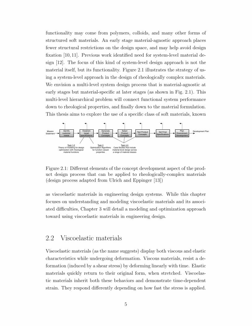
material itself, but its functionality. Figure 2.1 illustrates the strategy of us-

ing a system-level approach in the design of rheologically complex materials.

We envision a multi-level system design process that is material-agnostic at

early stages but material-specific at later stages (as shown in Fig. 2.1). This

multi-level hierarchical problem will connect functional system performance

down to rheological properties, and finally down to the material formulation.

This thesis aims to explore the use of a specific class of soft materials, known

Identify customer

needs

Establish target

specifications

Generate Product

Concepts

Select Product

ConceptsTest Product

ConceptsSet Final

SpecificationsPlan

DownstreamDevelopment

MissionStatement

Task 1-2Theory of modeling for design optimization with rheological

material functions

Task 3Optimization Algorithms

for function-valuedproperties

Task 4-5Case Studies that include

material-level design acrossa range of material classes

Development Plan

Figure 2.1: Different elements of the concept development aspect of the prod-uct design process that can be applied to rheologically-complex materials(design process adapted from Ulrich and Eppinger [13])

as viscoelastic materials in engineering design systems. While this chapter

focuses on understanding and modeling viscoelastic materials and its associ-

ated difficulties, Chapter 3 will detail a modeling and optimization approach

toward using viscoelastic materials in engineering design.

2.2 Viscoelastic materials

Viscoelastic materials (as the name suggests) display both viscous and elastic

characteristics while undergoing deformation. Viscous materials, resist a de-

formation (induced by a shear stress) by deforming linearly with time. Elastic

materials quickly return to their original form, when stretched. Viscoelas-

tic materials inherit both these behaviors and demonstrate time-dependent

strain. They respond differently depending on how fast the stress is applied.

5

For instance, if a silly putty (which is an example of a viscoelastic material)

is stretched slowly, the material elongates slowly and demonstrates a viscous

fluid-like behavior. On the other hand, if it is stretched too quickly, it breaks

without any displacement and behaves more like a solid. Thus, the strain is

dependent on the rate of the stress applied.

Viscoelasticity arises from the microstructure of the material. In the char-

acterization of viscoelastic materials, typically three important tensile tests

are performed, namely: (1) Creep Deformation (2) Stress Relaxation, and

(3) Dynamic Loading.

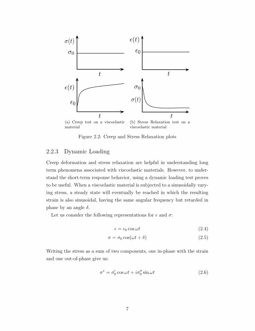
2.2.1 Creep

In the creep tests, the viscoelastic material is subjected to a steady uniaxial

stress σ0 and the resulting time-dependent strain ε(t) is studied. [14]

ε(t) = δ(t)/L0 (2.1)

If doubling the constant stress σ0 doubles the strain, then the material is

said to be linear i.e. displays a linear stress-strain relationship. The creep

compliance J(t) is then computed as the ratio between the strain and stress.

J(t) =ε(t)

σ0(2.2)

2.2.2 Stress relaxation

Another common test performed on viscoelastic materials is studying time-

dependent stress, σ(t) resulting from a constant strain, ε0. The relaxation

modulus K(t) is then computed as:

K(t) =σ(t)

ε0(2.3)

6

✏(t)

✏0

t

t

�0

�(t)

(a) Creep test on a viscoelasticmaterial

✏0

✏(t)

t

t

�0

�(t)

(b) Stress Relaxation test on aviscoelastic material

Figure 2.2: Creep and Stress Relaxation plots

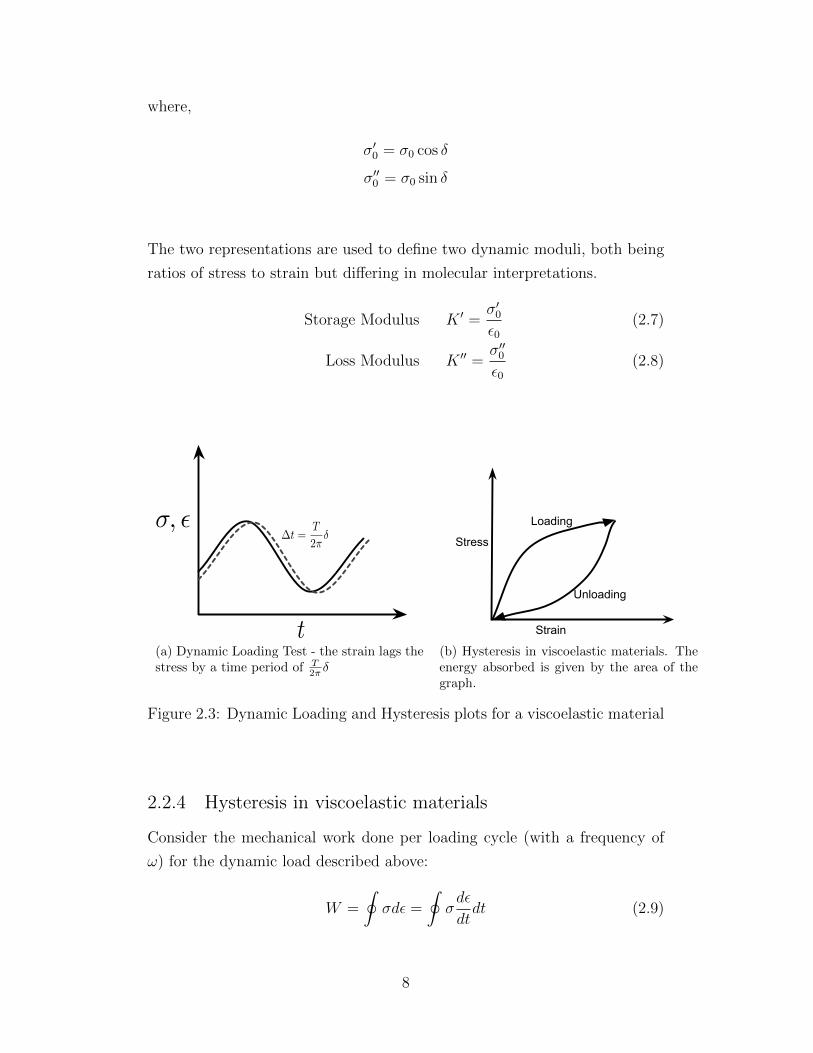
2.2.3 Dynamic Loading

Creep deformation and stress relaxation are helpful in understanding long

term phenomena associated with viscoelastic materials. However, to under-

stand the short-term response behavior, using a dynamic loading test proves

to be useful. When a viscoelastic material is subjected to a sinusoidally vary-

ing stress, a steady state will eventually be reached in which the resulting

strain is also sinusoidal, having the same angular frequency but retarded in

phase by an angle δ.

Let us consider the following representations for ε and σ:

ε = ε0 cosωt (2.4)

σ = σ0 cos(ωt+ δ) (2.5)

Writing the stress as a sum of two components, one in-phase with the strain

and one out-of-phase give us:

σ∗ = σ′0 cosωt+ iσ′′0 sinωt (2.6)

7

where,

σ′0 = σ0 cos δ

σ′′0 = σ0 sin δ

The two representations are used to define two dynamic moduli, both being

ratios of stress to strain but differing in molecular interpretations.

Storage Modulus K ′ =σ′0ε0

(2.7)

Loss Modulus K ′′ =σ′′0ε0

(2.8)

t

�, ✏�t =

T

2⇡�

(a) Dynamic Loading Test - the strain lags thestress by a time period of T

2π δ

Stress

Strain

Loading

Unloading

(b) Hysteresis in viscoelastic materials. Theenergy absorbed is given by the area of thegraph.

Figure 2.3: Dynamic Loading and Hysteresis plots for a viscoelastic material

2.2.4 Hysteresis in viscoelastic materials

Consider the mechanical work done per loading cycle (with a frequency of

ω) for the dynamic load described above:

W =

∮σdε =

∮σdε

dtdt (2.9)

8

With a time period T = 2π/ω, and using the expressions for ε from Eqn. 2.5

and σ from Eqn. 2.6, W can be evaluated as:

W =

∫ 2π/ω

0

(σ′0 cosωt)(−ε0ω sinωt)dt+

∫ 2π/ω

0

(σ′′0 sinωt)(−ε0ω sinωt)dt

(2.10)

Solving the integrals gives us:

W = 0− πσ′′0ε0 (2.11)

Thus, some energy is dissipated during the loading cycle. This phenomenon

is an example of hysteresis. Hysteresis in a system arises when the output

response of the system depends not only on the current but also past in-

puts, which in this case is due to the loss of some energy. The stress-strain

relationship during the loading cycle is show in Fig. 2.3(b).

Apart from viscoelastic systems, there are other engineering and biolog-

ical systems that exhibit other kinds of hysteresis such as electromagnets.

Hysteresis need not necessarily relate to the same underlying physical vari-

able. Viscoelastic materials undergo hysteresis based on the energy dissi-

pated during dynamic loading. In aircraft wing aerodynamics, hysteresis can

be observed when the angle of attack where the flow on top of the wing

reattaches is generally lower than the angle of attack where the flow sepa-

rates [15]. Physical adsorption is another example that exhibits the unusual

property, where it is possible to scan within the hysteresis loop by reversing

the direction of adsorption. [16].

2.2.5 Linear Viscoelasticity

A linear viscoelastic material is one which has a linear relationship between

its strain history and stress.

σ(t) =

∫ t

−∞K(t− t′)ε(t′)dt′ (2.12)

Here, K(t) is the relaxation modulus of the material, which is the function-

valued property that we will attempt to design. In other words this thesis

aims to identify an optimal shear modulus function for a material in order

to satisfy certain objectives (which will be explained with the help of a case

9

study in the following chapters). Though linear viscoelasticity is an idealized

representation of physical materials in the real world, it forms a good basis

to understand and study such complex rheological materials.

2.2.6 Mathematical models of viscoelastic materials

To ensure an optimal design of viscoelastic materials based on the functional-

ity it aims to serve, a mathematical model of the material is required. In this

section, a systematic approach is established for mathematically modeling

linear viscoelastic materials, for understanding the implications of general-

ized viscoelastic design and for addressing the challenges that its optimization

entails.

A common mechanical paradigm used in the study of viscoelastic models is

a combination of springs and dashpots. While a spring-dashpot model does

not directly represent the microstructure of viscoelastic materials, it helps us

visualize molecular motions. The spring (with a spring constant k) accounts

for the elastic component of the material and obeys Hookean spring laws.

σ = kε (2.13)

The spring constant k is analogous to the Young’s modulus E and σ and ε

are similar to the spring force and displacement respectively.

The viscous component is represented by a Newtonian dashpot (with a

viscosity c).

σ = cε (2.14)

The ratio between c and k is often used as a measure of viscoelastic response

time.

K0 =c

k(2.15)

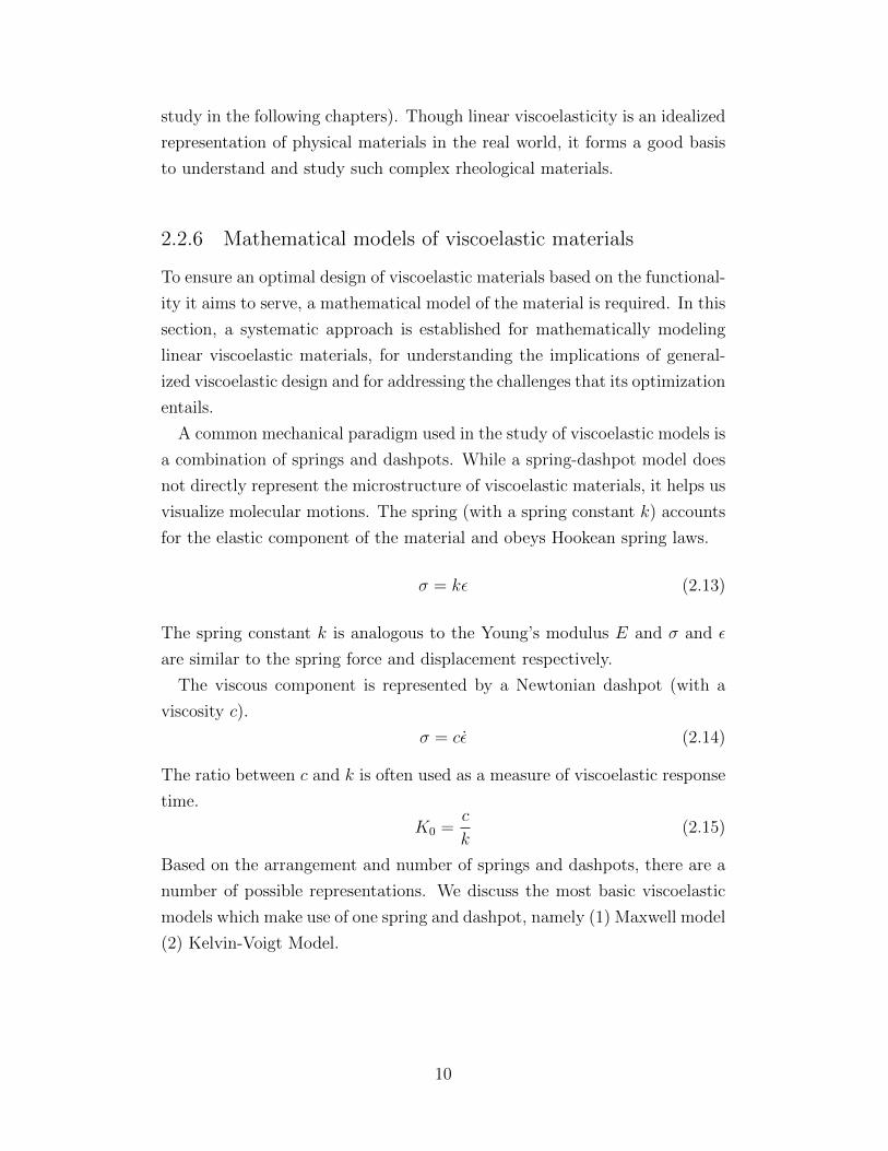
Based on the arrangement and number of springs and dashpots, there are a

number of possible representations. We discuss the most basic viscoelastic

models which make use of one spring and dashpot, namely (1) Maxwell model

(2) Kelvin-Voigt Model.

10

k c

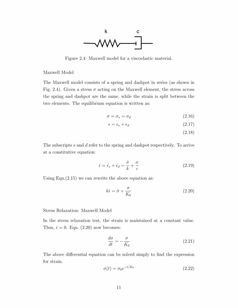
Figure 2.4: Maxwell model for a viscoelastic material.

Maxwell Model

The Maxwell model consists of a spring and dashpot in series (as shown in

Fig. 2.4). Given a stress σ acting on the Maxwell element, the stress across

the spring and dashpot are the same, while the strain is split between the

two elements. The equilibrium equation is written as:

σ = σs = σd (2.16)

ε = εs + εd (2.17)

(2.18)

The subscripts s and d refer to the spring and dashpot respectively. To arrive

at a constitutive equation:

ε = εs + εd =σ

k+σ

c(2.19)

Using Eqn.(2.15) we can rewrite the above equation as:

kε = σ +σ

K0

(2.20)

Stress Relaxation: Maxwell Model

In the stress relaxation test, the strain is maintained at a constant value.

Thus, ε = 0. Eqn. (2.20) now becomes:

dσ

dt= − σ

K0

(2.21)

The above differential equation can be solved simply to find the expression

for strain.

σ(t) = σ0e−t/K0 (2.22)

11

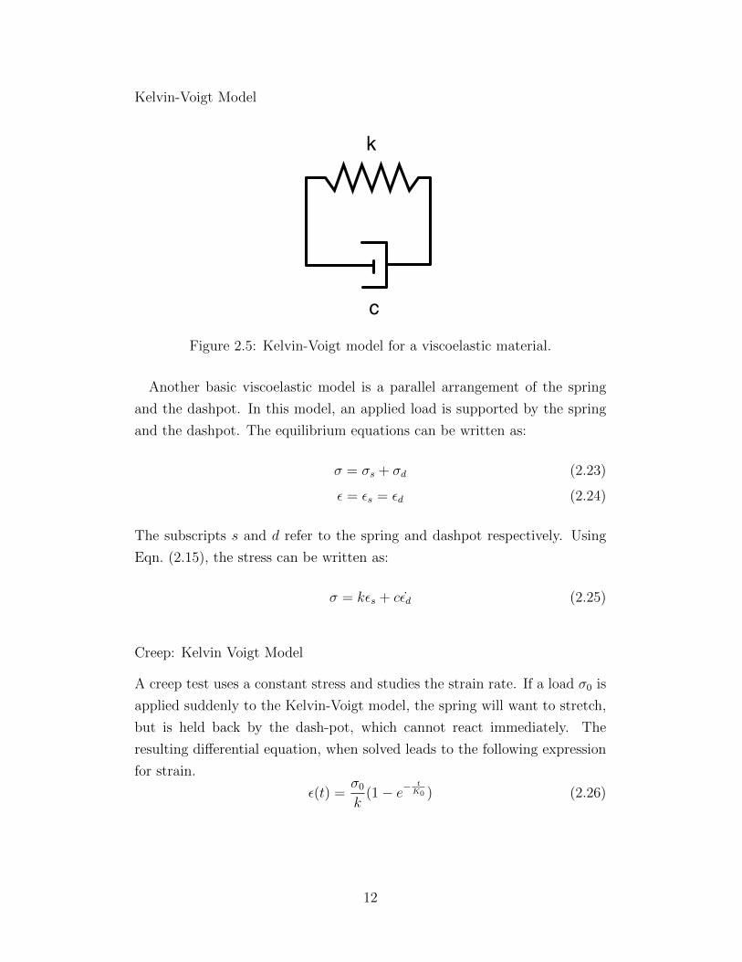
Kelvin-Voigt Model

k

c

Figure 2.5: Kelvin-Voigt model for a viscoelastic material.

Another basic viscoelastic model is a parallel arrangement of the spring

and the dashpot. In this model, an applied load is supported by the spring

and the dashpot. The equilibrium equations can be written as:

σ = σs + σd (2.23)

ε = εs = εd (2.24)

The subscripts s and d refer to the spring and dashpot respectively. Using

Eqn. (2.15), the stress can be written as:

σ = kεs + cεd (2.25)

Creep: Kelvin Voigt Model

A creep test uses a constant stress and studies the strain rate. If a load σ0 is

applied suddenly to the Kelvin-Voigt model, the spring will want to stretch,

but is held back by the dash-pot, which cannot react immediately. The

resulting differential equation, when solved leads to the following expression

for strain.

ε(t) =σ0k

(1− e−t

K0 ) (2.26)

12

2.2.7 Motivation to study viscoelastic materials

Having understood viscoelastic behavior, it is important to understand why

they should be studied. They are widely prevalent in biological, engineering,

and other physical systems. The disks in the human spine are viscoelastic

and undergo creep due to body weight. They grow shorter with time. Lying

down reduces the stress on the disks and thereby helps them recover. Most

people are hence taller in the mornings than in the evening. Astronauts

gained up to 5 cm under zero gravity conditions [14].

Creep is also the reason behind the sagging of wooden structures over

time. Polymer foam cushions used on couches and chairs also undergo creep

on prolonged application of pressure and conform to the shape of the person

sitting on them. Such is the case with metal turbine blades in jet engines,

which reach very high temperatures and need to withstand very high tensile

stresses. Conventional metals can creep significantly at high temperatures.

A newly born baby's head is viscoelastic and its ability to creep and recover

helps in the birthing process. If the baby sleeps in a particular position for

long, its head can become misshapen due to creep deformation. Bolts and

screws used in machine components, when subjected to high temperatures,

undergo stress relaxation and loosen over time [14].

Understanding the behavior of viscoelastic materials is the first step to uti-

lizing them in engineering design. Leveraging viscoelastic response to design

better engineering systems is the goal of this research work. Viscoelastic ma-

terials are excellent impact absorbers. Viscoelastic materials are used in car

bumpers, on computer drives to protect from mechanical shock, in helmets

(the foam padding inside), in wrestling mats, etc. They are also used in shoe

insoles to reduce impact transmitted to a person’s foot. Acoustic blankets

made of viscoelastic materials is used to attenuate the noise from helicopters.

Dampers made of such materials are also used to protect high rise buildings

from the impact of turbulent winds.

Chapters 3, 4 and 5 will detail the use of viscoelastic materials in engineer-

ing design and the optimization techniques that can be utilized in identifying

optimal material functions, thus enabling material-agnostic design and en-

hancing design freedom.

13

CHAPTER 3

Design Optimization via materialfunction targets

The first step to understanding material design optimization is to identify the

material property that we wish to control. In other words, our aim is to design

a viscoelastic material property function which will achieve certain design

objectives. For instance, in the design of a shock absorber with viscoelastic

materials, if we choose our material function as the relaxation modulus K(t),

we would then formulate our optimization problem to identify an optimal

target function K(t) that would minimize the shock (physically quantified as

acceleration).

As a preliminary step of implementing functionality-driven viscoelastic de-

sign, we utilize existing viscoelastic models and parameterizations of K(t).

While this serves as a good exercise to understanding the system and its

optimal target function, we identify the need to incorporate generalized vis-

coelastic design, that does not involve any a priori assumptions on K(t).

The use of optimal control methods in the identification of optimal material

target functions is also discussed in this chapter.

3.1 Relaxation Modulus as the target function

As defined in Chapter 2, the relaxation modulus of a viscoelastic material

is the ratio between the stress and the constant strain in a stress relaxation

test.

K(t) =σ(t)

ε0(3.1)

Here we consider one-dimensional deformation, and thus are able to repre-

sent the force through the viscoelastic connection with a single scalar equa-

14

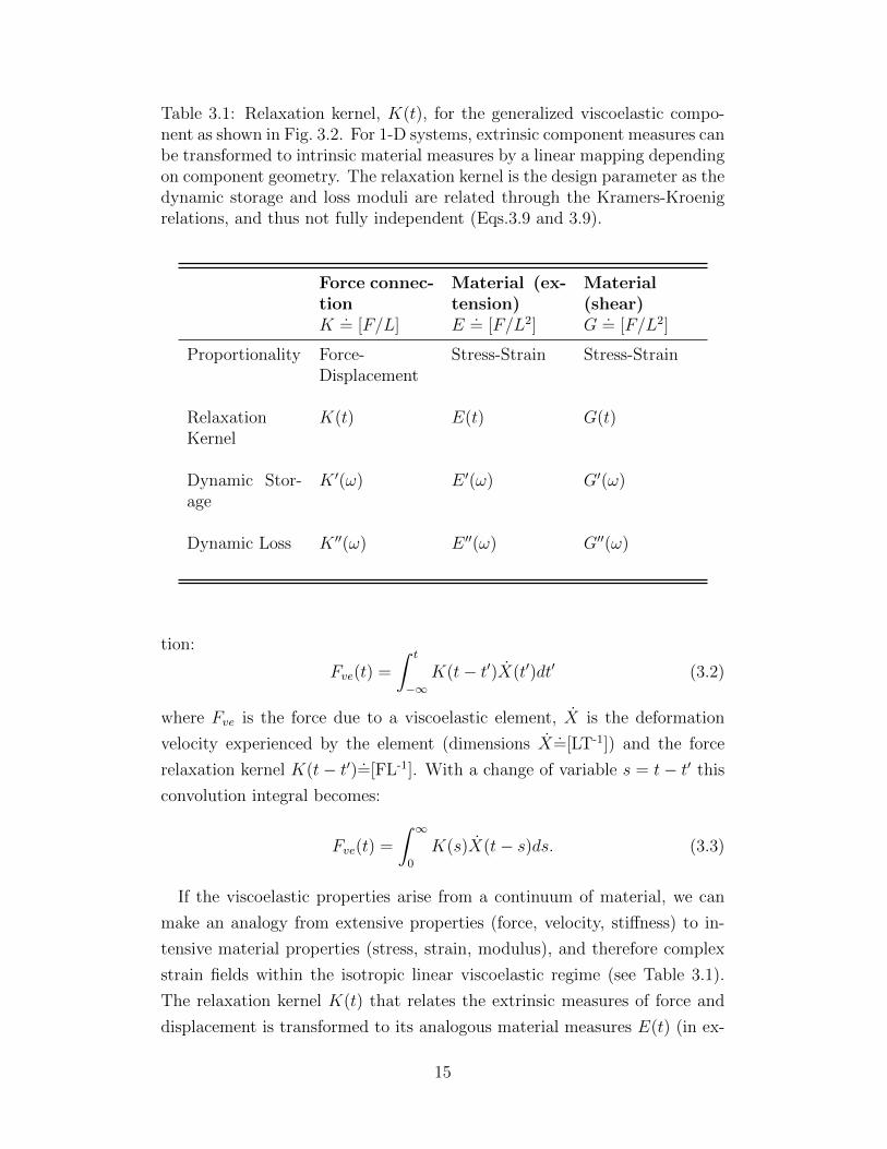
Table 3.1: Relaxation kernel, K(t), for the generalized viscoelastic compo-nent as shown in Fig. 3.2. For 1-D systems, extrinsic component measures canbe transformed to intrinsic material measures by a linear mapping dependingon component geometry. The relaxation kernel is the design parameter as thedynamic storage and loss moduli are related through the Kramers-Kroenigrelations, and thus not fully independent (Eqs.3.9 and 3.9).

Force connec-tionK

.= [F/L]

Material (ex-tension)E

.= [F/L2]

Material(shear)G

.= [F/L2]

Proportionality Force-Displacement

Stress-Strain Stress-Strain

RelaxationKernel

K(t) E(t) G(t)

Dynamic Stor-age

K ′(ω) E ′(ω) G′(ω)

Dynamic Loss K ′′(ω) E ′′(ω) G′′(ω)

tion:

Fve(t) =

∫ t

−∞K(t− t′)X(t′)dt′ (3.2)

where Fve is the force due to a viscoelastic element, X is the deformation

velocity experienced by the element (dimensions X=[LT-1]) and the force

relaxation kernel K(t− t′)=[FL-1]. With a change of variable s = t− t′ this

convolution integral becomes:

Fve(t) =

∫ ∞

0

K(s)X(t− s)ds. (3.3)

If the viscoelastic properties arise from a continuum of material, we can

make an analogy from extensive properties (force, velocity, stiffness) to in-

tensive material properties (stress, strain, modulus), and therefore complex

strain fields within the isotropic linear viscoelastic regime (see Table 3.1).

The relaxation kernel K(t) that relates the extrinsic measures of force and

displacement is transformed to its analogous material measures E(t) (in ex-

15

tension) or G(t) (in shear) which relate the intrinsic measures of stress and

strain through a linear mapping of area divided by length (dimensions [L])

based on geometry. A simple example of the relationship between the ex-

trinsic and intrinsic measures is shown in one-dimensional tension where

the intrinsic measures stress and strain are related through material con-

nection function E (Table 3.1) by σ = Eε. Converting these measures to

their extrinsic equivalents requires the geometrical relations σ = F/A and

ε = x/L. Combining these relations leads to the extrinsic form of Hooke’s

law, F = (EA/L)x. Where the extrinsic force connection kernel K can be

written as K = EA/L.= [F/L].

In the isotropic, incompressible, linear viscoelastic regime, the descriptive

kernel function, the stress relaxation modulus, is the measured stress response

to a step change in strain, which can be used generally in Boltzmann super-

postion [4,17]. The modulus is equivalent to a predictive constitutive model

parameter, and can be used to compute any three-dimensional deformation

history. By analogy to Eqn. (3.2), the 3-D expression for the Boltzmann

superposition integral uses the relaxation modulus G(t), in tensorial form:

σ(t) =

∫ t

−∞G(t− t′)γ(t′)dt′, (3.4)

where σ(t) is the Cauchy stress tensor, and the strain-rate tensor is:

γ = ∇ v + (∇ v)T, (3.5)

where v is the velocity field and we define the velocity gradient as (∇ v)ij =

∂vj/∂xi. Equation (3.4) is limited to small deformation in the linear vis-

coelastic regime for incompressible materials, but applies for any class of

linear viscoelastic material (elastomer, composite, polymeric liquid, colloid,

gel, etc.) falling within the framework of a continuum description.

The relaxation kernel K(t) is treated here as an independent design vari-

able. Alternative viscoelastic material functions, such as the creep compli-

ance J(t), can also be used to define a relation similar to Eqn. (3.4) with the

displacement field as the output of the integral. This may be mathematically

convenient for load-control inputs. However, in the linear viscoelastic limit,

all of the the material functions are interrelated [18], and therefore only one

single-valued function can be specified in the design.

16

Linear viscoelastic materials are commonly described in the frequency-

domain, such as the dynamic storage and loss moduli are shown in Table

3.1. For a viscoelastic fluid (with stress relaxing to zero at infinite time) the

dynamic storage and loss moduli are directly related to K(t) as

K ′(ω) = ω

∫ ∞

0

K(s) sin(ωs)ds (3.6)

K ′′(ω) = ω

∫ ∞

0

K(s) cos(ωs)ds. (3.7)

Additionally, the dynamic storage and loss moduli are combined to create a

complex modulus of the form K∗ = K ′ + iK ′′ where i is the imaginary unit.

Since each function is related to K(t), the two functions are clearly not

independent. As shown in Table 3.1, this holds true in the analogous material

measures in extension (E(t), E ′(ω), E ′′(ω)) and shear (G(t), G′(ω), G′′(ω)).

The interrelations are given by the Kramers-Kronig relations, shown here in

terms of the dynamic moduli [17]

G′(ω)−G′(∞) =2

π

∫ ∞

0

xG′′(x)

ω2 − x2dx (3.8)

G′′(ω) =2ω

π

∫ ∞

0

G′(x)

x2 − ω2dx (3.9)

where we define:

G′(∞) = limω→∞

G′(ω) (3.10)

Any in-phase and out-of-phase dynamic material functions must also sat-

isfy these relations. With simple shear properties, this includes moduli G′

and G′′, viscosities η′ and η′′, compliances J ′ and J ′′, and fluidities φ′ and

φ′′ [17,19]. The Kramers-Kronig relations also restrict the independent spec-

ification of frequency-dependent magnitude and phase angle.

The independent function K(t) (or equivalently G(t) or E(t)) is therefore

treated as the function-valued design variable for linear viscoelasticity.

17

3.2 Parameterizations of K(t)

In general, the relaxation kernel, K(t), can be treated as a function of ar-

bitrary structure. Passive materials or systems impose the restriction that

the function be monotonically decreasing [20, 21], however, this restriction

on complexity could be lifted through the use of actively controlled systems.

Complete freedom in the shape of the relaxation kernel presents difficulties

for numerical optimization. For this initial exploration of K(t) optimization,

we consider several parameterizations of K(t) with a finite number of design

parameters as shown in Fig. 3.4: parameterization as a dashpot, a single and

multi-mode Maxwell, and power law relaxation (analogous to a critical gel

material) [22,23].

For a standard, linear dashpot, the form of the relaxation kernel can be

represented as:

K(t) = c · δ(t) (3.11)

where c.= [F/ (L/T )] The dynamic coefficients for a linear dashpot are given

by

K ′(ω) = 0 (3.12)

K ′′(ω) = c · ω (3.13)

By analogy, a Newtonian fluid has G(t) = η0δ(t), G′ = 0, and G′′ = η0ω.

A Maxwell element is a linear spring and dashpot connected in series. It is

the simplest model of a viscoelastic fluid. The model can be generalized to a

multi-mode Maxwell model that includes M Maxwell elements connected in

parallel. The relaxation kernel, also known as a Prony series, is defined by:

K(t) =M∑

m=1

Kme−t/λm . (3.14)

where Km are the Maxwell spring constants (Km.= [F/L]), and λm are the

relaxation times (λm.= [T ]). The Maxwell dashpot coefficient is ηm = Kmλm.

Here we will consider the cases of M = 1 and M = 3 in order to limit the

number of parameters (2M parameters for an M -mode Maxwell model). For

18

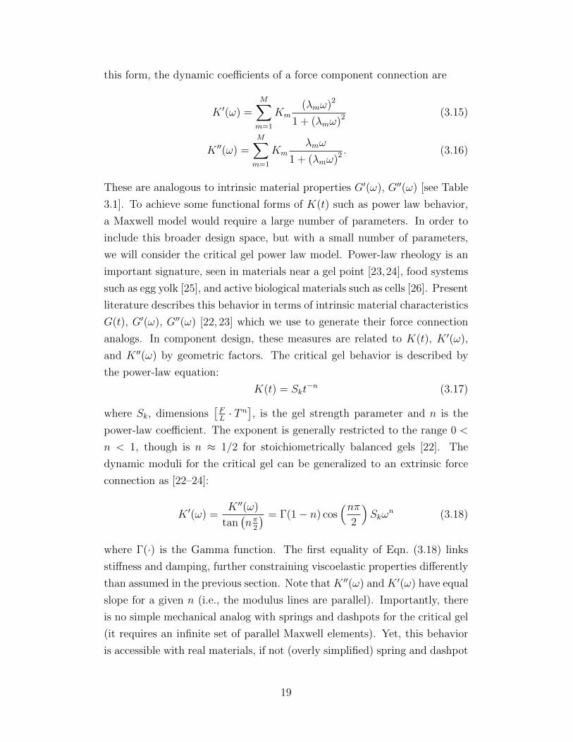
this form, the dynamic coefficients of a force component connection are

K ′(ω) =M∑

m=1

Km(λmω)2

1 + (λmω)2(3.15)

K ′′(ω) =M∑

m=1

Kmλmω

1 + (λmω)2. (3.16)

These are analogous to intrinsic material properties G′(ω), G′′(ω) [see Table

3.1]. To achieve some functional forms of K(t) such as power law behavior,

a Maxwell model would require a large number of parameters. In order to

include this broader design space, but with a small number of parameters,

we will consider the critical gel power law model. Power-law rheology is an

important signature, seen in materials near a gel point [23,24], food systems

such as egg yolk [25], and active biological materials such as cells [26]. Present

literature describes this behavior in terms of intrinsic material characteristics

G(t), G′(ω), G′′(ω) [22, 23] which we use to generate their force connection

analogs. In component design, these measures are related to K(t), K ′(ω),

and K ′′(ω) by geometric factors. The critical gel behavior is described by

the power-law equation:

K(t) = Skt−n (3.17)

where Sk, dimensions[FL· T n

], is the gel strength parameter and n is the

power-law coefficient. The exponent is generally restricted to the range 0 <

n < 1, though is n ≈ 1/2 for stoichiometrically balanced gels [22]. The

dynamic moduli for the critical gel can be generalized to an extrinsic force

connection as [22–24]:

K ′(ω) =K ′′(ω)

tan(nπ

2

) = Γ(1− n) cos(nπ

2

)Skω

n (3.18)

where Γ(·) is the Gamma function. The first equality of Eqn. (3.18) links

stiffness and damping, further constraining viscoelastic properties differently

than assumed in the previous section. Note that K ′′(ω) and K ′(ω) have equal

slope for a given n (i.e., the modulus lines are parallel). Importantly, there

is no simple mechanical analog with springs and dashpots for the critical gel

(it requires an infinite set of parallel Maxwell elements). Yet, this behavior

is accessible with real materials, if not (overly simplified) spring and dashpot

19

models.

0 2 4 6 8 10

0

1

Das

hpot

Maxwell element(s)

R

elax

atio

n ke

rnel

, K(t)

[a

rb. f

orce

or s

tress

]

Time (s)

Critical gel

/

-n

log-log

Figure 3.1: Parameterizations of the relaxation kernel, K(t), for a generallinear viscoelastic fluid model into numerous linear viscoelastic models toreduce the complexity of the design space. The viscoelsatic models usedto parameterize the relaxation modulus of the added viscoelastic compo-nent are: (i) a linear dashpot (solid), (ii) a Maxwell element (linear springand dashpot connected in series) single mode (dash-dot), (iii) Multi-modeMaxwell element, (short dash-dot), and (iv) a critical gel model, mechanicalspring-dashpot analog is not applicable (dash). Inset plot is double-log plotof the same curves with the Maxwell model characteristic timescale λ (as inEqn. (3.14)) and the critical gel exponent n (as in Eqn. (3.17)) labeled forreference [27].

While some parameterizations (i.e., Maxwell model) imply the use of a

specified topology of linear springs and dashpots, this is not generally nec-

essary for a viscoelastic connection. One could also parameterize K(t) as a

spline, or a discrete vector of independent points. This would be the ideal

approach, with maximum design freedom, which is discussed in the following

sections.

20

3.3 Generalized viscoelastic model

In the most general case, the optimization problem considered here seeks to

minimize an objective function that describes the performance of the overall

system and depends on the choice of K(t). Since the optimization is per-

formed with respect to K(t), which is a function-valued design variable, this

problem would fall under the class of optimal control problems [28]. While

there are well-established methods to solve these types of problems [29, 30],

the structure arising from the problem is complex due to the characteristic

convolution integrals and is not yet well understood.

While previous studies have addressed viscoelastic material design, many

have excluded the important feature of frequency dependence, resulting in

limited design freedom, and thus do not capitalize on the valuable ability

of viscoelastic materials to adjust properties with changes in loading fre-

quency [31]. Other work involves time dependent behavior, but specifies

that the linear viscoelastic functions be described by a superposition of ex-

ponential functions [32, 33]. The rigidity of this functional form limits the

design space and will require large numbers of parameters. For example,

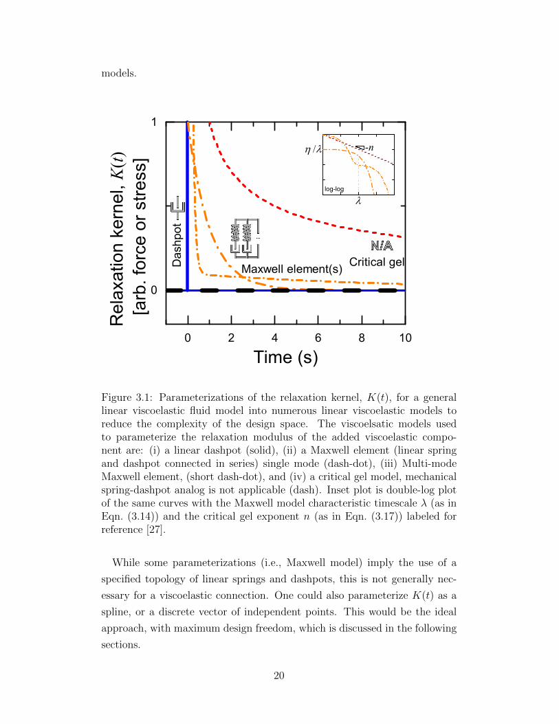
using a discrete topology as shown in Fig. 3.2, restricts design freedom. This

can be addressed by the introduction of a generalized viscoelastic element

which makes the design space continuous. To implement an early-stage ap-

proach that supports more flexible design exploration, we consider a linear

viscoelastic element where general mechanical response is described by ex-

perimentally measurable material functions that depend only on a timescale,

the relaxation kernel, K(t). Overall system performance can then be opti-

mized by considering K(t) as the design variable. The optimal function K(t)

can then serve as a target function in efforts to formulate a material that

leads to optimal system performance.

Considering one-dimensional deformation as mentioned in Eqn. (3.19), we

have:

FV E(t) =

∫ ∞

0

K(s)x(t− s)ds. (3.19)

The convolution integral in Equation 3.19 presents a numerical challenge

in optimization since the instantaneous state variables of the system cannot

be represented by independent derivative functions, as the integral is not

separable. In this thesis, we focus on the case where K(t) is a general con-

21

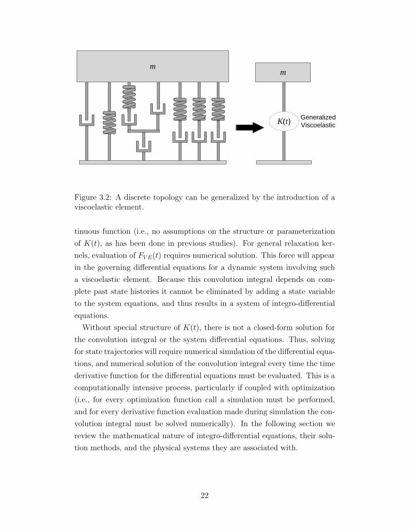
Generalized

Viscoelastic

m

K(t)

m

Figure 3.2: A discrete topology can be generalized by the introduction of aviscoelastic element.

tinuous function (i.e., no assumptions on the structure or parameterization

of K(t), as has been done in previous studies). For general relaxation ker-

nels, evaluation of FV E(t) requires numerical solution. This force will appear

in the governing differential equations for a dynamic system involving such

a viscoelastic element. Because this convolution integral depends on com-

plete past state histories it cannot be eliminated by adding a state variable

to the system equations, and thus results in a system of integro-differential

equations.

Without special structure of K(t), there is not a closed-form solution for

the convolution integral or the system differential equations. Thus, solving

for state trajectories will require numerical simulation of the differential equa-

tions, and numerical solution of the convolution integral every time the time

derivative function for the differential equations must be evaluated. This is a

computationally intensive process, particularly if coupled with optimization

(i.e., for every optimization function call a simulation must be performed,

and for every derivative function evaluation made during simulation the con-

volution integral must be solved numerically). In the following section we

review the mathematical nature of integro-differential equations, their solu-

tion methods, and the physical systems they are associated with.

22

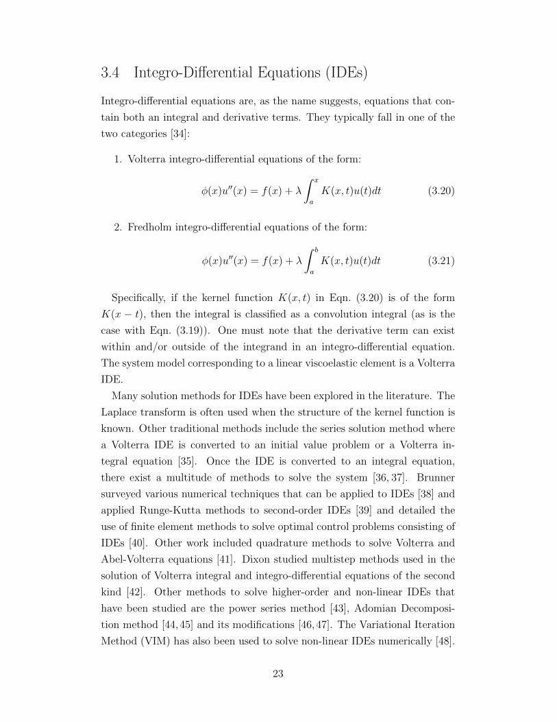
3.4 Integro-Differential Equations (IDEs)

Integro-differential equations are, as the name suggests, equations that con-

tain both an integral and derivative terms. They typically fall in one of the

two categories [34]:

1. Volterra integro-differential equations of the form:

φ(x)u′′(x) = f(x) + λ

∫ x

a

K(x, t)u(t)dt (3.20)

2. Fredholm integro-differential equations of the form:

φ(x)u′′(x) = f(x) + λ

∫ b

a

K(x, t)u(t)dt (3.21)

Specifically, if the kernel function K(x, t) in Eqn. (3.20) is of the form

K(x − t), then the integral is classified as a convolution integral (as is the

case with Eqn. (3.19)). One must note that the derivative term can exist

within and/or outside of the integrand in an integro-differential equation.

The system model corresponding to a linear viscoelastic element is a Volterra

IDE.

Many solution methods for IDEs have been explored in the literature. The

Laplace transform is often used when the structure of the kernel function is

known. Other traditional methods include the series solution method where

a Volterra IDE is converted to an initial value problem or a Volterra in-

tegral equation [35]. Once the IDE is converted to an integral equation,

there exist a multitude of methods to solve the system [36, 37]. Brunner

surveyed various numerical techniques that can be applied to IDEs [38] and

applied Runge-Kutta methods to second-order IDEs [39] and detailed the

use of finite element methods to solve optimal control problems consisting of

IDEs [40]. Other work included quadrature methods to solve Volterra and

Abel-Volterra equations [41]. Dixon studied multistep methods used in the

solution of Volterra integral and integro-differential equations of the second

kind [42]. Other methods to solve higher-order and non-linear IDEs that

have been studied are the power series method [43], Adomian Decomposi-

tion method [44,45] and its modifications [46,47]. The Variational Iteration

Method (VIM) has also been used to solve non-linear IDEs numerically [48].

23

Jiang et al. propose a convolution integral method to simulate real-time hy-

brid systems [49]. Edwards analysed the numerical simulation of Volterra

IDEs [50]. Most of these efforts, however, do not focus on convolution kernel

solution or using IDEs in conjunction with engineering design optimization.

3.4.1 Modeling Convolution Kernels in IDEs

Several methods of convolution quadrature have been studied, which is im-

portant for numerical evaluation of hysteretic systems. Lubich, a pioneer of

the convolution quadrature, uses Laplace transforms to determine quadrature

weights [51]. Lubich et al. also applied quadrature to fractional IDEs [52].

However, in these cases the structure of the kernel functions K(x − t) was

known a priori. Zhang et al. proposed using a combination of linear meth-

ods with compound quadrature rules [53]. Finite elements were also used

for this purpose when the system involved modeling of flow and partial dif-

ferential equations [54, 55]. These efforts form a strong mathematical basis

to understand convolution kernels and IDEs, but in general do not address

rate-dependent convolution kernels of the form given in Eqn. (3.19), and do

not extend their use in engineering design optimization.

In this thesis we introduce the use of optimal control in the optimization

of viscoelastic systems (characterized by convolution IDEs), specifically for

the case of general relaxation kernels K(t). Optimal control methods have

successfully been used in the optimization of similar systems, such as wave

energy converters [56] where the cost functional term has a rate-dependent

convolution structure. Yu and Falnes approached the problem by using a

state space approximation of the convolution term; this approximation results

in additional system model states [57]. The objective of this study is to

identify a generalized form of the shear relaxation modulus K(t) found in

Eqn. (3.19) to support more flexible design strategies for early-stage design

exploration involving viscoelastic materials. This flexibility may help reduce

design fixation and enhance design innovation using rheologically complex

materials.

24

3.5 Optimal Control methods

The desired early-stage design approach that is not restricted by a priori ma-

terial class choices (i.e., material agnostic) requires a generalized treatment

of K(t). Instead of parameterizing K(t) and tuning parameters to improve

system performance, we propose to design K(t) directly. In other words,

instead of specifying a finite set of parameters as design variables, we choose

to design with respect to an infinite-dimensional (function-valued) quantity.

Optimal control methods provide the ability to solve infinite-dimensional

optimization problems.

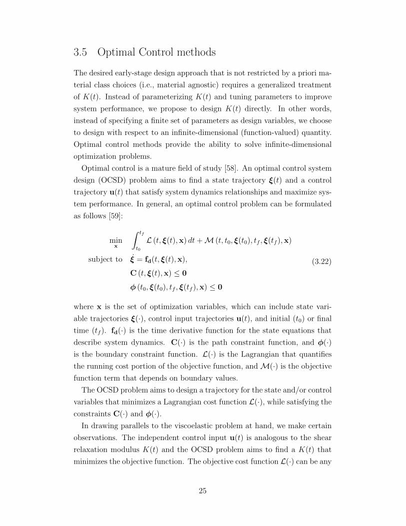
Optimal control is a mature field of study [58]. An optimal control system

design (OCSD) problem aims to find a state trajectory ξ(t) and a control

trajectory u(t) that satisfy system dynamics relationships and maximize sys-

tem performance. In general, an optimal control problem can be formulated

as follows [59]:

minx

∫ tf

t0

L (t, ξ(t),x) dt+M (t, t0, ξ(t0), tf , ξ(tf ),x)

subject to ξ = fd(t, ξ(t),x),

C (t, ξ(t),x) ≤ 0

φ (t0, ξ(t0), tf , ξ(tf ),x) ≤ 0

(3.22)

where x is the set of optimization variables, which can include state vari-

able trajectories ξ(·), control input trajectories u(t), and initial (t0) or final

time (tf ). fd(·) is the time derivative function for the state equations that

describe system dynamics. C(·) is the path constraint function, and φ(·)is the boundary constraint function. L(·) is the Lagrangian that quantifies

the running cost portion of the objective function, andM(·) is the objective

function term that depends on boundary values.

The OCSD problem aims to design a trajectory for the state and/or control

variables that minimizes a Lagrangian cost function L(·), while satisfying the

constraints C(·) and φ(·).In drawing parallels to the viscoelastic problem at hand, we make certain

observations. The independent control input u(t) is analogous to the shear

relaxation modulus K(t) and the OCSD problem aims to find a K(t) that

minimizes the objective function. The objective cost function L(·) can be any

25

function of the state and control variables. For instance, in its use in vibration

damping, the objective of the OCSD problem could be to minimize the peak

amplitude of displacement. The state trajectories ξ(t) in this example could

be the displacement or velocity vectors. fd(·) represents the system dynamics

of the viscoelastic system and would include the viscoelastic force described

in Eqn. (3.19). One may have boundary constraints on the initial and final

states of the system. Path constraints may exist when the state or control

trajectories are required to follow a target trajectory shape. This might be

relevant in the case of designing a physically realizable K(t).

3.5.1 Solution Methods for Optimal Control System design

This subsection discusses the solution methods adopted for OCSD problems.

Following a brief insight into these methods, we will discuss the key differ-

ences between the standard OCSD problem and the viscoelastic design prob-

lem. There are two classes of methods employed to solve OCSD problems:

(1) indirect and (2) direct optimal control methods.

Indirect Optimal Control

Indirect methods are based on the calculus of variations, and work by apply-

ing optimality conditions to the optimal control problem to form a boundary

value problems (BVP). In simple cases the BVP may be solved analyti-

cally, but in more general cases it must be discretized and solved numer-

ically [60]. The general algorithm of an indirect method is optimize-then-

discretize (O → D).

Indirect approaches help provide insights into the structure of the solution,

but usually the analytical derivatives are challenging to calculate. In the case

of expensive or black-box functions, derivatives are numerically calculated.

Direct Optimal Control

Direct optimal control methods take the opposite approach, where the opti-

mal control problem is discretized in time first, i.e. discretize-then-optimize

(D → O). The result is a nonlinear program (NLP) that can be solved using

26

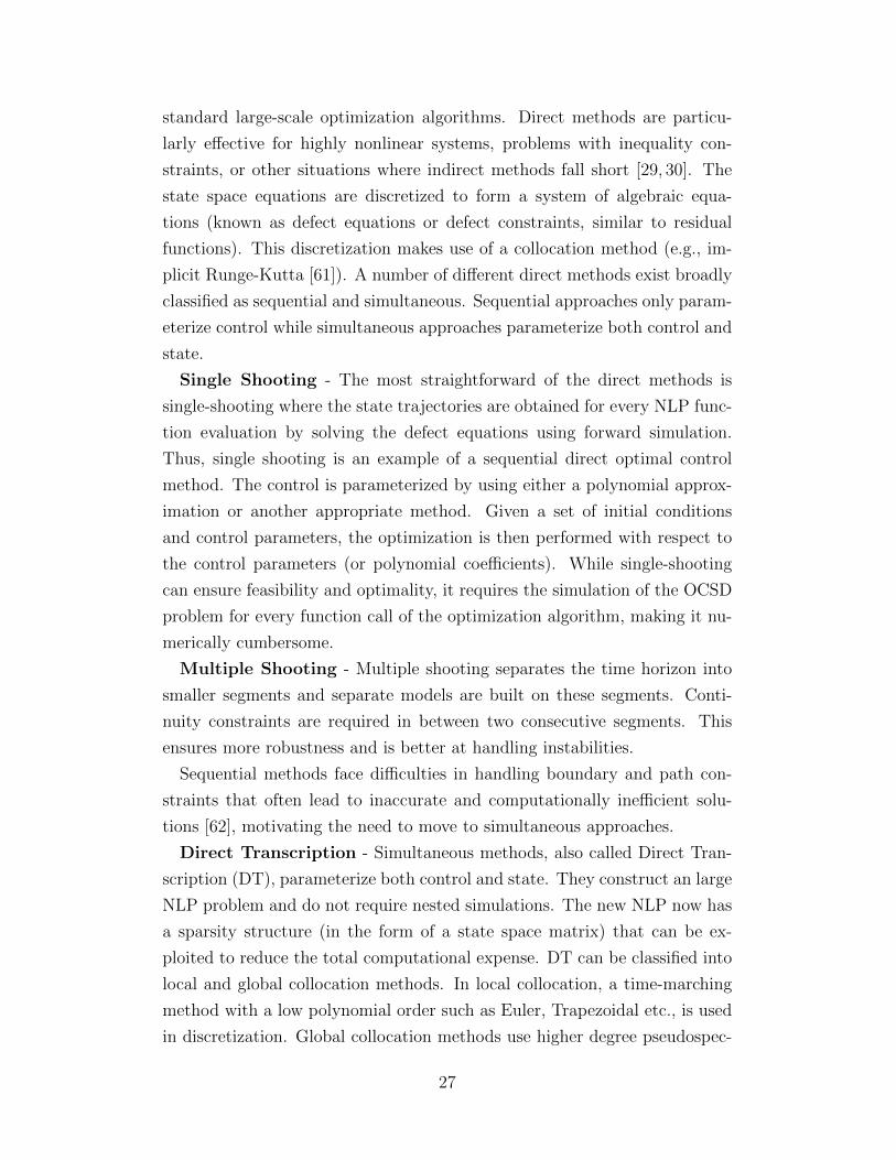
standard large-scale optimization algorithms. Direct methods are particu-

larly effective for highly nonlinear systems, problems with inequality con-

straints, or other situations where indirect methods fall short [29, 30]. The

state space equations are discretized to form a system of algebraic equa-

tions (known as defect equations or defect constraints, similar to residual

functions). This discretization makes use of a collocation method (e.g., im-

plicit Runge-Kutta [61]). A number of different direct methods exist broadly

classified as sequential and simultaneous. Sequential approaches only param-

eterize control while simultaneous approaches parameterize both control and

state.

Single Shooting - The most straightforward of the direct methods is

single-shooting where the state trajectories are obtained for every NLP func-

tion evaluation by solving the defect equations using forward simulation.

Thus, single shooting is an example of a sequential direct optimal control

method. The control is parameterized by using either a polynomial approx-

imation or another appropriate method. Given a set of initial conditions

and control parameters, the optimization is then performed with respect to

the control parameters (or polynomial coefficients). While single-shooting

can ensure feasibility and optimality, it requires the simulation of the OCSD

problem for every function call of the optimization algorithm, making it nu-

merically cumbersome.

Multiple Shooting - Multiple shooting separates the time horizon into

smaller segments and separate models are built on these segments. Conti-

nuity constraints are required in between two consecutive segments. This

ensures more robustness and is better at handling instabilities.

Sequential methods face difficulties in handling boundary and path con-

straints that often lead to inaccurate and computationally inefficient solu-

tions [62], motivating the need to move to simultaneous approaches.

Direct Transcription - Simultaneous methods, also called Direct Tran-

scription (DT), parameterize both control and state. They construct an large

NLP problem and do not require nested simulations. The new NLP now has

a sparsity structure (in the form of a state space matrix) that can be ex-

ploited to reduce the total computational expense. DT can be classified into

local and global collocation methods. In local collocation, a time-marching

method with a low polynomial order such as Euler, Trapezoidal etc., is used

in discretization. Global collocation methods use higher degree pseudospec-

27

tral methods that result in a higher accuracy [59].

It is easy to make observations on the similarities between the standard

OCSD problem and the viscoelastic formulation. However it is important to

understand the subtle differences that exist in the viscoelastic problem. As

discussed in the previous sub-section, the convolution integral poses signifi-

cant challenges in the modeling of viscoelastic material based systems. One

place where this challenge shows up is in the structure of the OCSD problem.

With the use of the viscoelastic element, the viscoelastic force in Eqn. (3.19)

typically appears in the derivative function equation, fd(·). Discretizing FV E

in time using a convolution sum would result in:

FV E[k] =

∫ tk

0

K(s)x(t− s)ds =k∑

i=0

K[i]x[k − i+ 1] (3.23)

where k denotes the kth time step representing the time instant tk. We can

see from this discretization that we would require a summation of FV E over

all the time instants prior to tk. This is atypical of a standard optimal control

problem, where the states and derivative functions usually depend only on

the current and the immediate previous time-step.

Another subtle difference is in the direction of the time marching between

the state and control. Usually, in a standard OCSD problems, both state and

control march forward in time. In the viscoelastic problem we can see that

the control, K(t) and the state, x(t), convolve in time. In graphical terms,

the convolution of teo functions f and g, is written as f ∗ g. It is defined

as the integral of the product of the two functions after one is reversed and

shifted. For example, consider the convolution of the unit impulse function

with the exponential function:

f(t) = u(t) (3.24)

g(t) = e−tu(t) (3.25)

where

u(t) =

{1 : t ≥ 0

0 : t < 0

28

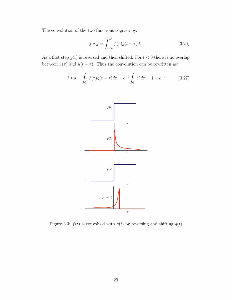
The convolution of the two functions is given by:

f ∗ g =

∫ ∞

−∞f(τ)g(t− τ)dτ (3.26)

As a first step g(t) is reversed and then shifted. For t < 0 there is no overlap

between u(τ) and u(t− τ). Thus the convolution can be rewritten as:

f ∗ g =

∫ t

0

f(τ)g(t− τ)dτ = e−t∫ t

0

eτdτ = 1− e−t (3.27)

f(t)

g(t)

f(⌧)

g(t � ⌧)

t

⌧

t

⌧

Figure 3.3: f(t) is convolved with g(t) by reversing and shifting g(t)

29

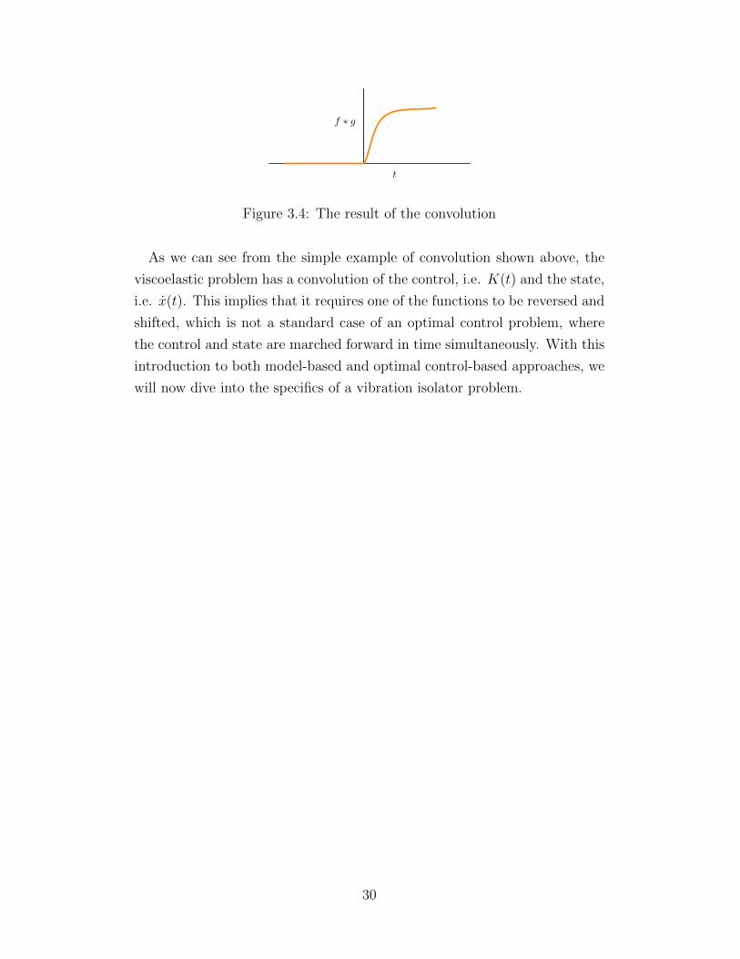
f ⇤ g

t

Figure 3.4: The result of the convolution

As we can see from the simple example of convolution shown above, the

viscoelastic problem has a convolution of the control, i.e. K(t) and the state,

i.e. x(t). This implies that it requires one of the functions to be reversed and

shifted, which is not a standard case of an optimal control problem, where

the control and state are marched forward in time simultaneously. With this

introduction to both model-based and optimal control-based approaches, we

will now dive into the specifics of a vibration isolator problem.

30

CHAPTER 4

Numerical Studies on a vibrationisolator - Part 1

In this chapter, the use of viscoelastic materials in engineering design is

demonstrated with a case study involving a vibration isolator design. Ini-

tially, the study is conducted using existing viscoelastic models such as

Maxwell, Critical Gel and the optimal paramters of design are identified

for each viscoelast model. In Chapter 5, the study is then extended to en-

tail generalized viscoelastic design, free from parameterizations and optimal

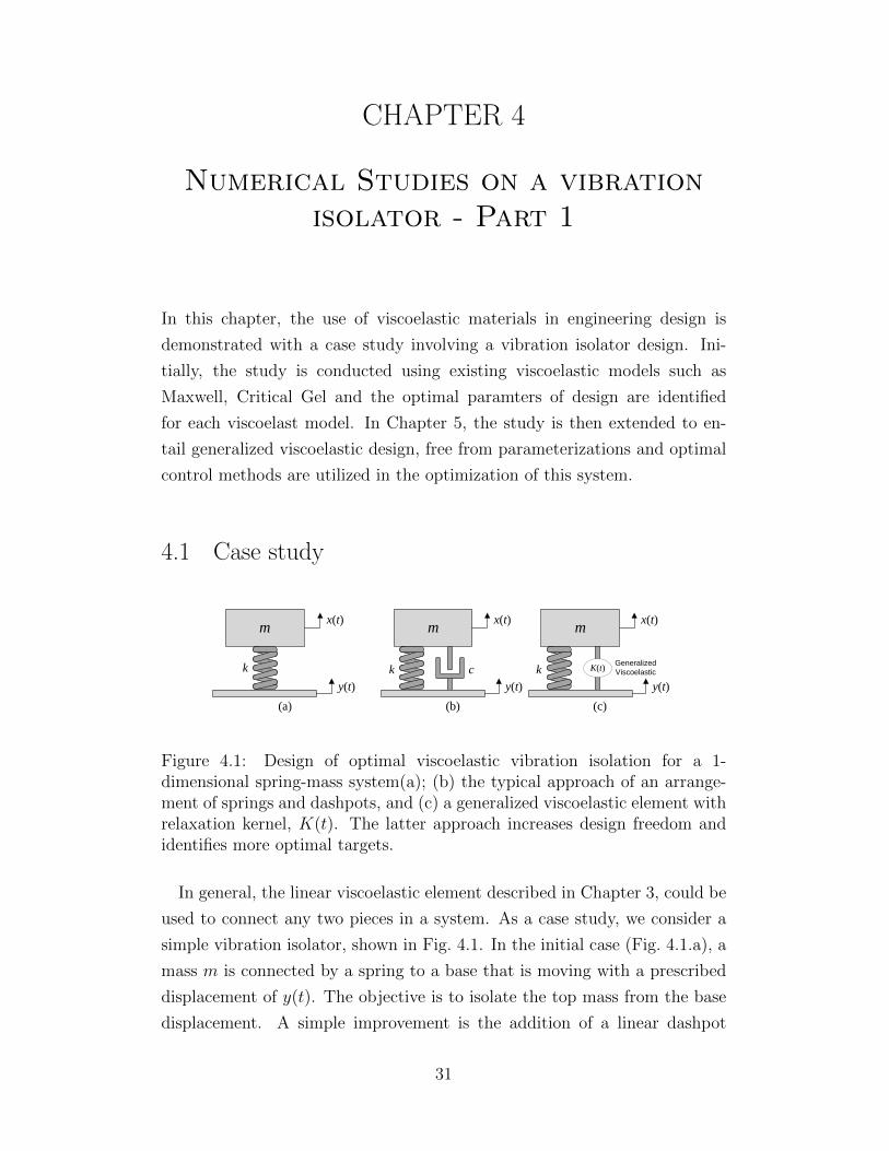
control methods are utilized in the optimization of this system.

4.1 Case study

m

y(t)

x(t)

Generalized

Viscoelastick K(t)

(c)

m

y(t)

x(t)

ck

(b)(a)

m

k

y(t)

x(t)

Figure 4.1: Design of optimal viscoelastic vibration isolation for a 1-dimensional spring-mass system(a); (b) the typical approach of an arrange-ment of springs and dashpots, and (c) a generalized viscoelastic element withrelaxation kernel, K(t). The latter approach increases design freedom andidentifies more optimal targets.

In general, the linear viscoelastic element described in Chapter 3, could be

used to connect any two pieces in a system. As a case study, we consider a

simple vibration isolator, shown in Fig. 4.1. In the initial case (Fig. 4.1.a), a

mass m is connected by a spring to a base that is moving with a prescribed

displacement of y(t). The objective is to isolate the top mass from the base

displacement. A simple improvement is the addition of a linear dashpot

31

(Fig. 4.1.b). We will generalize the linear dashpot to be a parallel viscoelastic

connection with relaxation kernel K(t), described in Chapter 3. We will

demonstrate the added performance from a viscoelastic connection (shown

in Fig. 4.1c), and optimize K(t) based on the parameterizations described in

Sec. 3.2.

4.1.1 Governing Equations

Given an initial condition Fve(t = 0) = 0, Eqn. (3.19) has limits of integration

from 0 to t. In general, the expression requires convolution of the kernel

function K(t) with the entire time-history of the velocity experienced by the

element, x(t).

For the particular system in Fig. 4.1.c, with a generalized viscoelastic el-

ement and the initial condition Fve(t = 0) = 0, the governing equation for

conservation of linear momentum is most generally written as:

− k(x− y)−∫ t

0

K(s) [x(t− s)− y(t− s)] ds = mx(t) (4.1)

where s = t− t′ and x− y = X, or the velocity of deformation, as defined in

Eqn. (3.19).

The convolution integral structure has two important consequences. First,

the equations cannot be written in matrix form. Second, the numerical sim-

ulation of this model requires increased computation at each time step, since

each time derivative function evaluation requires an integration of the en-

tire prior time-history of velocities. This is an important challenge to be

addressed for general design of K(t), and is discussed in Chapter 5. Here,

we simplify the analysis by considering time-periodic solutions for which the

convolution integral simplifies. Consider a time-periodic prescribed base exci-

tation, y(t) = Y sin(ωt). For a linear system, the steady-state displacement

response of x(t) will be time-periodic at the forcing frequency [63]. The

known structure of this harmonic solution will simplify the convolution in-

tegral terms, to an extent that we can write the governing equations as a

function of instantaneous state variables. Thus, integral calculations of K(t)

terms are not required at each time step.

32

Using complex notation, the displacement of the mass has the form:

x(t) = Im{x∗eiωt

}(4.2)

where Im{} takes the imaginary portion of the complex quantity. The

coefficients are:

x∗ = XR + iXi (4.3)

By substituting Eqns. (4.2) and (4.3) into Eqn. (4.1), a linear system of

two equations and two unknowns will result. The system of equations takes

the form:

Mx = B. (4.4)

The unknowns are

x = [XR, Xi]T (4.5)

The nonhomogeneous portion is:

B = [−Y (ωS + k),−Y ωC] (4.6)

and the 2 by 2 matrix is given by:

M =

[(mω2 − ωS − k) (ωC)

(−ωC) (mω2 − ωS − k)

](4.7)

The scalar coefficients C and S require integral calculations that depend on

the kernel function K(t),

C(ω) =

∫ ∞

0

K(s) cos(ωs)ds (4.8)

S(ω) =

∫ ∞

0

K(s) sin(ωs)ds. (4.9)

Comparing this result to Eqn. (3.6) and Eqn. (3.7) shows that these integrals

are related to the dynamic material functions as

C = K ′′(ω)/ω (4.10)

S = K ′(ω)/ω. (4.11)

The primary design variable is still K(s), since it gives the rheological signa-

33

ture of both dynamic moduli, and the dynamic moduli are not independent

parameters due to the Kramers-Kronig relations in Eqn. (3.9).

The solutions to the governing equations give |x|, the displacement am-

plitude of the mass, as a function of frequency. Normalizing this result by

the input displacement amplitude, Y , leads to the non-dimensionalized am-

plitude.

|x| = |x|Y

(4.12)

From the displacement, the acceleration amplitude of the mass is defined to

be:

|x| = ω2|x| (4.13)

Equivalently, it can be non-dimensionalized by the problem inputs of dis-

palcement (Y.= [length]), mass (m

.= [mass]), and spring constant (k

.=[

masstime

2]) as:

|˜x| = |x|Y(km

) (4.14)

In generalK(t) can take any form, but hereK(t) is parameterized using the

methods described in Section 3.2. The response ˜x is optimized by minimizing

the peak value with respect to a finite set of design variables that parame-

terize K(t). These parameters can themselves be non-dimensionalized as fol-

lows. For the linear dashpot, c = c/√km; for the Maxwell model, λ = λ/

√m/k

and η = η/√km; and for the critical gel, S = S/k

12(2+n)

mn/2 1Y

(note that the critical

gel exponent, n, is dimensionless).

The objective function f for the design optimization problem here is the

maximum non-dimensionalized acceleration amplitude.

f(x) = max |˜x| (4.15)

4.2 Results

Relaxing the design space to include even simple parameterizations of vis-

coelastic fluids can change the behavior of the vibration isolator, as demon-

strated in Fig. 4.2. While parametrization does not provide infinite design

freedom, it is valuable for this initial treatment, as it allows a visualization

of the extended design space. A Maxwell model allows for the introduction

34

10-1 100 101 102 10310-3

10-2

10-1

100

101

102

103

x

n

1

10-1 100 101 102 10310-4

10-3

10-2

10-1

100

101

102

103

-1

-2

-2 n-2

x

(b)

(a)

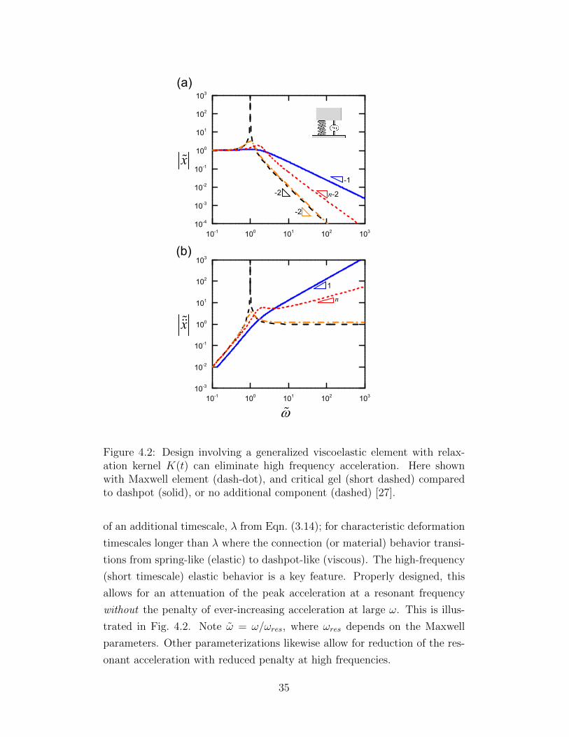
Figure 4.2: Design involving a generalized viscoelastic element with relax-ation kernel K(t) can eliminate high frequency acceleration. Here shownwith Maxwell element (dash-dot), and critical gel (short dashed) comparedto dashpot (solid), or no additional component (dashed) [27].

of an additional timescale, λ from Eqn. (3.14); for characteristic deformation

timescales longer than λ where the connection (or material) behavior transi-

tions from spring-like (elastic) to dashpot-like (viscous). The high-frequency

(short timescale) elastic behavior is a key feature. Properly designed, this

allows for an attenuation of the peak acceleration at a resonant frequency

without the penalty of ever-increasing acceleration at large ω. This is illus-

trated in Fig. 4.2. Note ω = ω/ωres, where ωres depends on the Maxwell

parameters. Other parameterizations likewise allow for reduction of the res-

onant acceleration with reduced penalty at high frequencies.

35

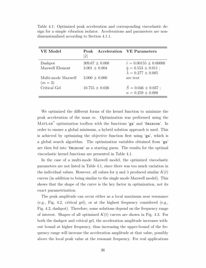
Table 4.1: Optimized peak acceleration and corresponding viscoelastic de-sign for a simple vibration isolator. Accelerations and parameters are non-dimensionalized according to Section 4.1.1.

VE Model Peak Acceleration|˜x|

VE Parameters

Dashpot 309.67 ± 0.000 c = 0.00155 ± 0.00000Maxwell Element 3.001 ± 0.004 η = 0.553 ± 0.011 ;

λ = 0.277 ± 0.005Multi-mode Maxwell(m = 3)

3.000 ± 0.000 see text

Critical Gel 10.755 ± 0.026 S = 0.046 ± 0.037 ;n = 0.259 ± 0.008

We optimized the different forms of the kernel function to minimize the

peak acceleration of the mass m. Optimization was performed using the

Matlab™ optimization toolbox with the functions ‘ga’ and ‘fmincon’. In

order to ensure a global minimum, a hybrid solution approach is used. This

is achieved by optimizing the objective function first using ‘ga’, which is

a global search algorithm. The optimization variables obtained from ‘ga’

are then fed into ‘fmincon’ as a starting guess. The results for the optimal

viscoelastic kernel functions are presented in Table 4.1.

In the case of a multi-mode Maxwell model, the optimized viscoelastic

parameters are not listed in Table 4.1, since there was too much variation in

the individual values. However, all values for η and λ produced similar K(t)

curves (in addition to being similar to the single mode Maxwell model). This

shows that the shape of the curve is the key factor in optimization, not its

exact parametrization.

The peak amplitude can occur either as a local maximum near resonance

(e.g., Fig. 4.2, critical gel), or at the highest frequency considered (e.g.,

Fig. 4.2, dashpot). Therefore, some solutions depend on the frequency range

of interest. Shapes of all optimized K(t) curves are shown in Fig. 4.3. For

both the dashpot and critical gel, the acceleration amplitude increases with-

out bound at higher frequency, thus increasing the upper-bound of the fre-

quency range will increase the acceleration amplitude at that value, possibly

above the local peak value at the resonant frequency. For real applications

36

a finite range of frequency is reasonable, e.g., excitation amplitudes decrease

and may be negligible above a critical frequency.

Introducing a linear viscoelastic connection decreases the peak accelera-

tion beyond that of a simple linear dashpot. With the introduction of a

characteristic timescale, a Maxwell model provided the most improvement

compared to the conventional method. A critical gel element also provides

a marked improvement. Surprisingly, in this simplified problem, additional

design freedom in the form of additional viscoelastic parameters (i.e. a multi-

mode Maxwell model) does not provide further improvement over a single

mode Maxwell model. This is likely due to the fact that this toy problem

has only one characteristic frequency, thus only one additional time scale is

necessary for optimal performance.

These results suggest that a critical gel model and multi-mode Maxwell

model may further improve performance for more complex problems involv-

ing a more complicated forcing function. More degrees of freedom and ad-

ditional characteristic timescales may prove beneficial in excitations that su-

perpose multiple frequencies, or structures with multiple vibration modes.

4.2.1 Case Study Extension

As an extension to the above results and in order to get a better intuition for

more practical systems, the dynamic vibration isolator was further general-

ized to consider a range of non-dimensional natural frequencies ω∗ for which

a single viscoelastic element is used. This natural frequency is normalized

by some reference spring-mass system (k0, m0) such that:

ω∗ =ω∗

ω0

(4.16)

where ω0 is the natural frequency of the reference system ω0 =√k0/m0.

This is analogous to a “one size fits all” damper where the primary mass

and spring may vary by application (Fig. 4.4). As shown before, use and op-

timization of a generalized viscoelastic element for a fixed natural frequency

(i.e. ω∗ = 1), significantly improves the system response. However, the bene-

fit of the optimized viscoelastic element is diluted for a system whose natural

frequency is different from that for which the system is optimized.

37

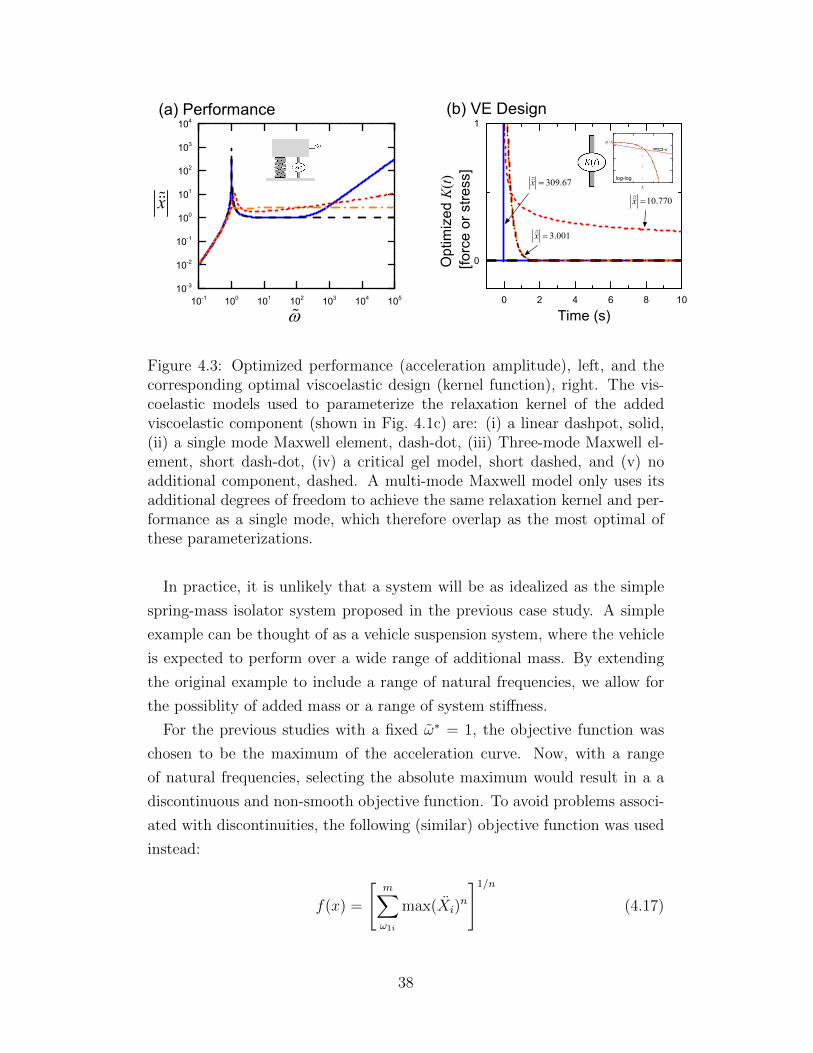
10-1 100 101 102 103 104 10510-3

10-2

10-1

100

101

102

103

104

x

0 2 4 6 8 10

0

1

Opt

imiz

ed K

(t)

[forc

e or

stre

ss]

Time (s)

3.001x

309.67x

10.770x

(b) VE Design

-n

log-log

/

(a) Performance

Figure 4.3: Optimized performance (acceleration amplitude), left, and thecorresponding optimal viscoelastic design (kernel function), right. The vis-coelastic models used to parameterize the relaxation kernel of the addedviscoelastic component (shown in Fig. 4.1c) are: (i) a linear dashpot, solid,(ii) a single mode Maxwell element, dash-dot, (iii) Three-mode Maxwell el-ement, short dash-dot, (iv) a critical gel model, short dashed, and (v) noadditional component, dashed. A multi-mode Maxwell model only uses itsadditional degrees of freedom to achieve the same relaxation kernel and per-formance as a single mode, which therefore overlap as the most optimal ofthese parameterizations.

In practice, it is unlikely that a system will be as idealized as the simple

spring-mass isolator system proposed in the previous case study. A simple

example can be thought of as a vehicle suspension system, where the vehicle

is expected to perform over a wide range of additional mass. By extending

the original example to include a range of natural frequencies, we allow for

the possiblity of added mass or a range of system stiffness.

For the previous studies with a fixed ω∗ = 1, the objective function was

chosen to be the maximum of the acceleration curve. Now, with a range

of natural frequencies, selecting the absolute maximum would result in a a

discontinuous and non-smooth objective function. To avoid problems associ-

ated with discontinuities, the following (similar) objective function was used

instead:

f(x) =

[m∑

ω1i

max(Xi)n

]1/n(4.17)

38

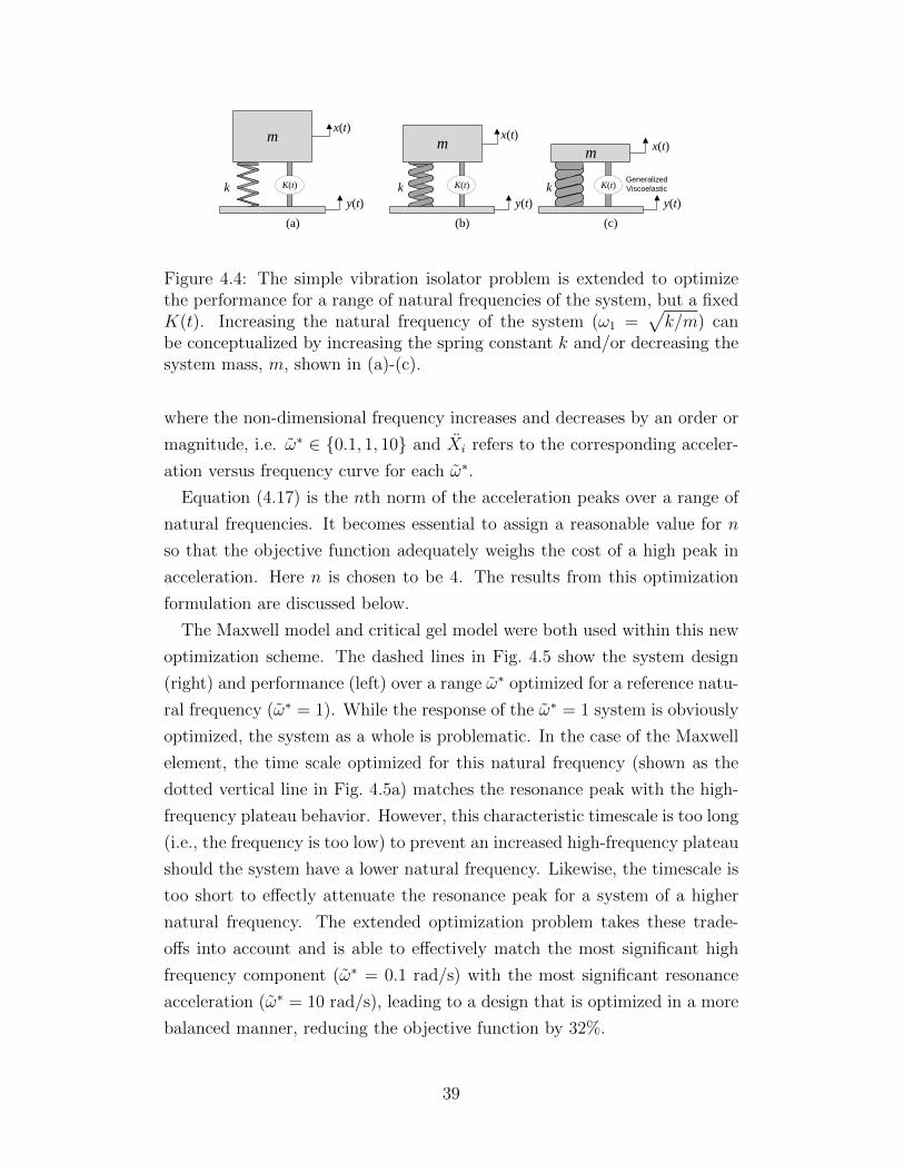
K(t) K(t)K(t)

m

y(t)

x(t)

Generalized

Viscoelastick

(c)

m

y(t)

x(t)

k

(b)(a)

m

k

y(t)

x(t)

Figure 4.4: The simple vibration isolator problem is extended to optimizethe performance for a range of natural frequencies of the system, but a fixedK(t). Increasing the natural frequency of the system (ω1 =

√k/m) can

be conceptualized by increasing the spring constant k and/or decreasing thesystem mass, m, shown in (a)-(c).

where the non-dimensional frequency increases and decreases by an order or

magnitude, i.e. ω∗ ∈ {0.1, 1, 10} and Xi refers to the corresponding acceler-

ation versus frequency curve for each ω∗.

Equation (4.17) is the nth norm of the acceleration peaks over a range of

natural frequencies. It becomes essential to assign a reasonable value for n

so that the objective function adequately weighs the cost of a high peak in

acceleration. Here n is chosen to be 4. The results from this optimization

formulation are discussed below.

The Maxwell model and critical gel model were both used within this new

optimization scheme. The dashed lines in Fig. 4.5 show the system design

(right) and performance (left) over a range ω∗ optimized for a reference natu-

ral frequency (ω∗ = 1). While the response of the ω∗ = 1 system is obviously

optimized, the system as a whole is problematic. In the case of the Maxwell

element, the time scale optimized for this natural frequency (shown as the

dotted vertical line in Fig. 4.5a) matches the resonance peak with the high-

frequency plateau behavior. However, this characteristic timescale is too long

(i.e., the frequency is too low) to prevent an increased high-frequency plateau

should the system have a lower natural frequency. Likewise, the timescale is

too short to effectly attenuate the resonance peak for a system of a higher

natural frequency. The extended optimization problem takes these trade-

offs into account and is able to effectively match the most significant high

frequency component (ω∗ = 0.1 rad/s) with the most significant resonance

acceleration (ω∗ = 10 rad/s), leading to a design that is optimized in a more

balanced manner, reducing the objective function by 32%.

39

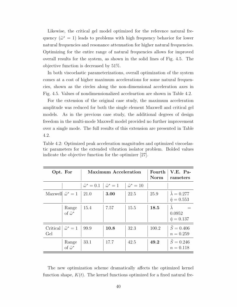
Likewise, the critical gel model optimized for the reference natural fre-

quency (ω∗ = 1) leads to problems with high frequency behavior for lower

natural frequencies and resonance attenuation for higher natural frequencies.

Optimizing for the entire range of natural frequencies allows for improved

overall results for the system, as shown in the solid lines of Fig. 4.5. The

objective function is decreased by 51%.

In both viscoelastic parameterizations, overall optimization of the system

comes at a cost of higher maximum accelerations for some natural frequen-

cies, shown as the circles along the non-dimensional acceleration axes in

Fig. 4.5. Values of nondimensionalized acceleartion are shown in Table 4.2.

For the extension of the original case study, the maximum acceleration

amplitude was reduced for both the single element Maxwell and critical gel

models. As in the previous case study, the additional degrees of design

freedom in the multi-mode Maxwell model provided no further improvement

over a single mode. The full results of this extension are presented in Table

4.2.

Table 4.2: Optimized peak acceleration magnitudes and optimized viscoelas-tic parameters for the extended vibration isolator problem. Bolded valuesindicate the objective function for the optimizer [27].

Opt. For Maximum Acceleration FourthNorm

V.E. Pa-rameters

ω∗ = 0.1 ω∗ = 1 ω∗ = 10

Maxwell ω∗ = 1 21.0 3.00 22.5 25.9 λ = 0.277η = 0.553

Rangeof ω∗

15.4 7.57 15.5 18.5 λ =0.0952η = 0.137

CriticalGel

ω∗ = 1 99.9 10.8 32.3 100.2 S = 0.406n = 0.259

Rangeof ω∗

33.1 17.7 42.5 49.2 S = 0.246n = 0.118

The new optimization scheme dramatically affects the optimized kernel

function shape, K(t). The kernel functions optimized for a fixed natural fre-

40

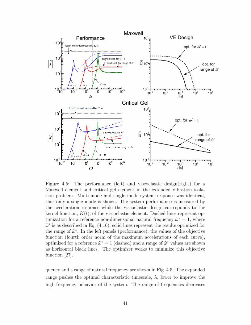
10-3 10-2 10-1 100 10110-1

100

101

*

* 1

t [s]

K(t) opt. for

range of

opt. for

Critical Gel

10-3 10-2 10-1 100 10110-1

100

101

*

* 1

K(t)

t [s]

opt. for range of

opt. for

VE Design

10-2 10-1 100 101 102 10310-1

100

101

102

*

* 10* 1

x

fourth norm decreases by 32%

solid: opt. for range of

dashed: opt. for

* 0.1

* 1

PerformanceMaxwell

Figure 4.5: The performance (left) and viscoelastic design(right) for aMaxwell element and critical gel element in the extended vibration isola-tion problem. Multi-mode and single mode system response was identical,thus only a single mode is shown. The system performance is measured bythe acceleration response while the viscoelastic design corresponds to thekernel function, K(t), of the viscoelastic element. Dashed lines represent op-timization for a reference non-dimensional natural frequency ω∗ = 1, whereω∗ is as described in Eq. (4.16); solid lines represent the results optimized forthe range of ω∗. In the left panels (performance), the values of the objectivefunction (fourth order norm of the maximum accelerations of each curve),optimized for a reference ω∗ = 1 (dashed) and a range of ω∗ values are shownas horizontal black lines. The optimizer works to minimize this objectivefunction [27].

quency and a range of natural frequency are shown in Fig. 4.5. The expanded

range pushes the optimal characteristic timescale, λ, lower to improve the

high-frequency behavior of the system. The range of frequencies decreases

41

the magnitude of n, the critical gel exponent, effectively making the system

more solid-like, again improving the high-frequency behavior of the system.

An important note to make is that these results, even more so than the

original problem, are dependent on the range of input frequency (ω) chosen.

The ever-increasing acceleration at high frequency for a liquid-like system as

well as a critical gel model drives the optimized results.

Passive vibration isolators find use in a variety of practical applications.

In their use as air isolators in large industrial equipment, the typical natural

frequency range is 1.5-3 Hz. In the case of base isolators used in buildings and

large structures, the natural frequency varies over a low seismic range. Their

usage in vehicles and aviation pertains to a frequency range of 10-20 Hz. The

key takeaway here is that real world vibration isolation occurs over not just

one but a range of resonant frequencies, for which viscoelastic responses can

be optimized.

Having established a good basis for using viscoelastic materials in a vibra-

tion isolator case study, we will now move on to generalizing the problem.

This is achieved by freeing K(t) of its model parameterizations and is dis-

cussed in detail in the upcoming chapter.

42

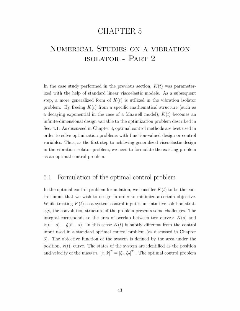
CHAPTER 5

Numerical Studies on a vibrationisolator - Part 2

In the case study performed in the previous section, K(t) was parameter-

ized with the help of standard linear viscoelastic models. As a subsequent

step, a more generalized form of K(t) is utilized in the vibration isolator

problem. By freeing K(t) from a specific mathematical structure (such as

a decaying exponential in the case of a Maxwell model), K(t) becomes an

infinite-dimensional design variable to the optimization problem described in

Sec. 4.1. As discussed in Chapter 3, optimal control methods are best used in

order to solve optimization problems with function-valued design or control

variables. Thus, as the first step to achieving generalized viscoelastic design

in the vibration isolator problem, we need to formulate the existing problem

as an optimal control problem.

5.1 Formulation of the optimal control problem

In the optimal control problem formulation, we consider K(t) to be the con-

trol input that we wish to design in order to minimize a certain objective.

While treating K(t) as a system control input is an intuitive solution strat-

egy, the convolution structure of the problem presents some challenges. The

integral corresponds to the area of overlap between two curves: K(s) and

x(t − s) − y(t − s). In this sense K(t) is subtly different from the control

input used in a standard optimal control problem (as discussed in Chapter

3). The objective function of the system is defined by the area under the

position, x(t), curve. The states of the system are identified as the position

and velocity of the mass m. [x, x]T = [ξ1, ξ2]T . The optimal control problem

43

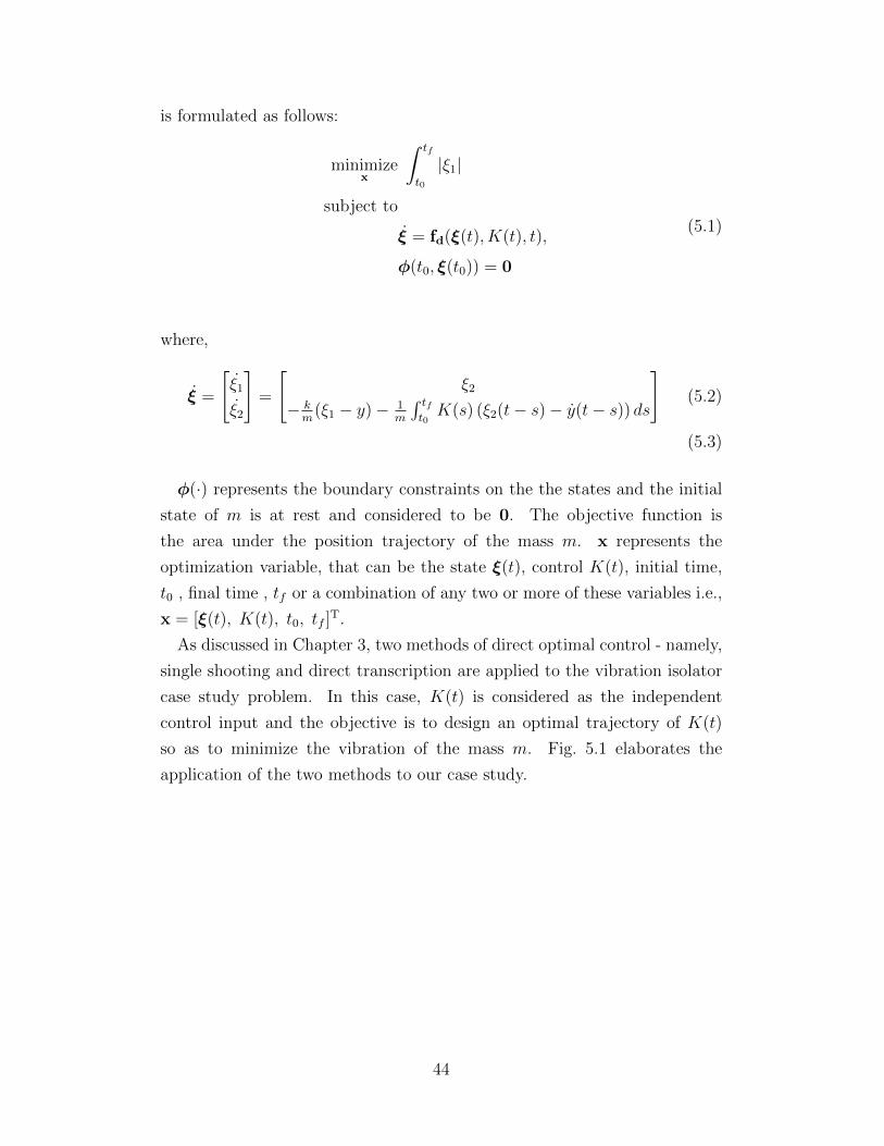
is formulated as follows:

minimizex

∫ tf

t0

|ξ1|

subject to

ξ = fd(ξ(t), K(t), t),

φ(t0, ξ(t0)) = 0

(5.1)

where,

ξ =

[ξ1

ξ2

]=

[ξ2

− km

(ξ1 − y)− 1m

∫ tft0K(s) (ξ2(t− s)− y(t− s)) ds

](5.2)

(5.3)

φ(·) represents the boundary constraints on the the states and the initial

state of m is at rest and considered to be 0. The objective function is

the area under the position trajectory of the mass m. x represents the

optimization variable, that can be the state ξ(t), control K(t), initial time,

t0 , final time , tf or a combination of any two or more of these variables i.e.,

x = [ξ(t), K(t), t0, tf ]T.

As discussed in Chapter 3, two methods of direct optimal control - namely,

single shooting and direct transcription are applied to the vibration isolator

case study problem. In this case, K(t) is considered as the independent

control input and the objective is to design an optimal trajectory of K(t)

so as to minimize the vibration of the mass m. Fig. 5.1 elaborates the

application of the two methods to our case study.

44

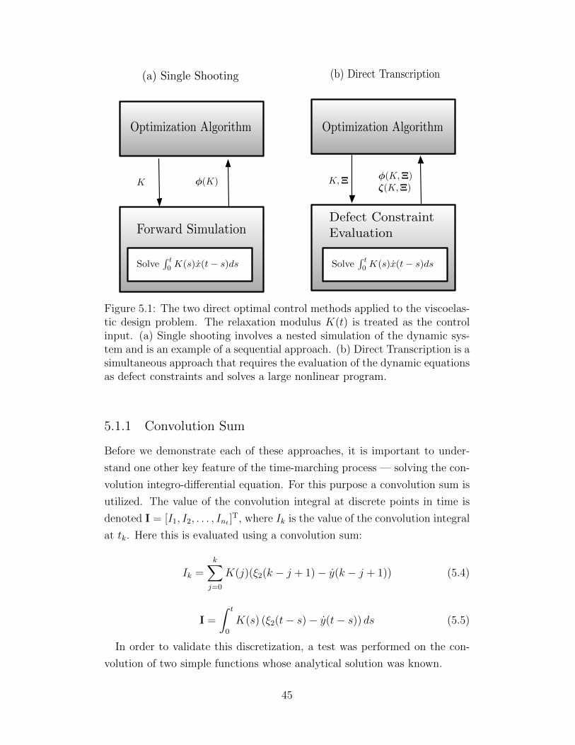
SolveR t0 K(s)x(t � s)ds

Forward Simulation

Optimization Algorithm Optimization Algorithm

SolveR t0 K(s)x(t � s)ds

Defect ConstraintEvaluation

�(K) K,⌅�(K,⌅)⇣(K,⌅)

K

(a) Single Shooting (b) Direct Transcription

Figure 5.1: The two direct optimal control methods applied to the viscoelas-tic design problem. The relaxation modulus K(t) is treated as the controlinput. (a) Single shooting involves a nested simulation of the dynamic sys-tem and is an example of a sequential approach. (b) Direct Transcription is asimultaneous approach that requires the evaluation of the dynamic equationsas defect constraints and solves a large nonlinear program.

5.1.1 Convolution Sum

Before we demonstrate each of these approaches, it is important to under-

stand one other key feature of the time-marching process — solving the con-

volution integro-differential equation. For this purpose a convolution sum is

utilized. The value of the convolution integral at discrete points in time is

denoted I = [I1, I2, . . . , Int ]T, where Ik is the value of the convolution integral

at tk. Here this is evaluated using a convolution sum:

Ik =k∑

j=0

K(j)(ξ2(k − j + 1)− y(k − j + 1)) (5.4)

I =

∫ t

0

K(s) (ξ2(t− s)− y(t− s)) ds (5.5)

In order to validate this discretization, a test was performed on the con-

volution of two simple functions whose analytical solution was known.

45

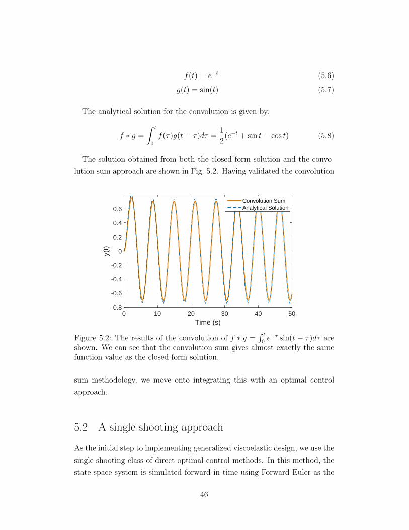
f(t) = e−t (5.6)

g(t) = sin(t) (5.7)

The analytical solution for the convolution is given by:

f ∗ g =

∫ t

0

f(τ)g(t− τ)dτ =1

2(e−t + sin t− cos t) (5.8)

The solution obtained from both the closed form solution and the convo-

lution sum approach are shown in Fig. 5.2. Having validated the convolution

Time (s)0 10 20 30 40 50

y(t)

-0.8

-0.6

-0.4

-0.2

0

0.2

0.4

0.6Convolution SumAnalytical Solution

Figure 5.2: The results of the convolution of f ∗ g =∫ t0e−τ sin(t − τ)dτ are

shown. We can see that the convolution sum gives almost exactly the samefunction value as the closed form solution.

sum methodology, we move onto integrating this with an optimal control

approach.

5.2 A single shooting approach

As the initial step to implementing generalized viscoelastic design, we use the

single shooting class of direct optimal control methods. In this method, the

state space system is simulated forward in time using Forward Euler as the

46

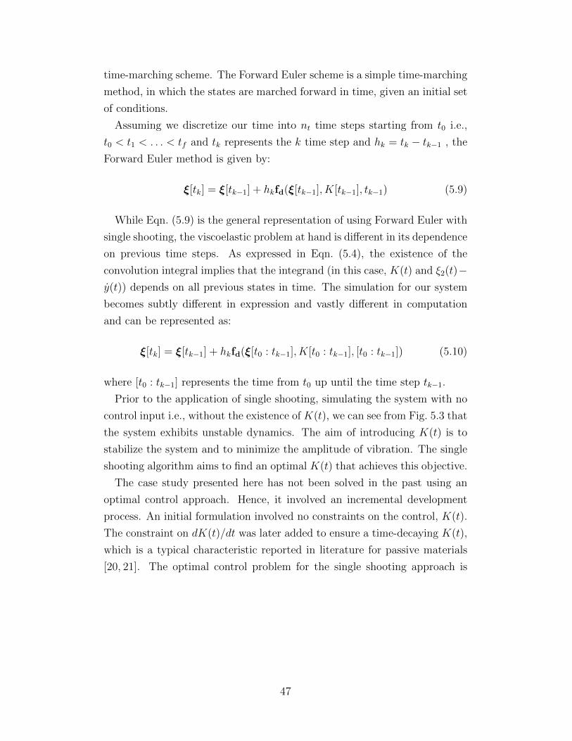
time-marching scheme. The Forward Euler scheme is a simple time-marching

method, in which the states are marched forward in time, given an initial set

of conditions.

Assuming we discretize our time into nt time steps starting from t0 i.e.,

t0 < t1 < . . . < tf and tk represents the k time step and hk = tk − tk−1 , the

Forward Euler method is given by:

ξ[tk] = ξ[tk−1] + hkfd(ξ[tk−1], K[tk−1], tk−1) (5.9)

While Eqn. (5.9) is the general representation of using Forward Euler with

single shooting, the viscoelastic problem at hand is different in its dependence

on previous time steps. As expressed in Eqn. (5.4), the existence of the

convolution integral implies that the integrand (in this case, K(t) and ξ2(t)−y(t)) depends on all previous states in time. The simulation for our system

becomes subtly different in expression and vastly different in computation

and can be represented as:

ξ[tk] = ξ[tk−1] + hkfd(ξ[t0 : tk−1], K[t0 : tk−1], [t0 : tk−1]) (5.10)

where [t0 : tk−1] represents the time from t0 up until the time step tk−1.

Prior to the application of single shooting, simulating the system with no

control input i.e., without the existence of K(t), we can see from Fig. 5.3 that

the system exhibits unstable dynamics. The aim of introducing K(t) is to

stabilize the system and to minimize the amplitude of vibration. The single

shooting algorithm aims to find an optimal K(t) that achieves this objective.

The case study presented here has not been solved in the past using an

optimal control approach. Hence, it involved an incremental development

process. An initial formulation involved no constraints on the control, K(t).

The constraint on dK(t)/dt was later added to ensure a time-decaying K(t),

which is a typical characteristic reported in literature for passive materials

[20, 21]. The optimal control problem for the single shooting approach is

47

Time(s)0 50 100 150 200

x(t)

-4000

-3000

-2000

-1000

0

1000

2000

3000

Figure 5.3: Unstable dynamics demonstrated by the vibration isolator sys-tem without the presence of a viscoelastic element. The plot represents theposition of mass m over time.

formulated as follows:

minK

∫ tf

t0

|ξ1|

subject to ξ(t0) = 0

dK(t)

dt≤ 0

(5.11)

where ξ = fd(ξ(t), K(t), t) is satisfied via simulation, and the time derivative

function is defined as:

fd(·) =

[ξ2

− km

(ξ1 − y)− 1m

∫ tft0K(s) (ξ2(t− s)− y(t− s)) ds

]

In this case K(t), is parameterized at uniformly discretized points in time:

K = [K(t1), K(t2), . . . , K(tnt)]T, and the optimization is performed with

respect to these nt discrete values. As a result the derivative constraint is

transformed into a set of linear algebraic inequality constraints.

48

5.3 Direct Transcription

In the DT formulation both the state and control trajectories are discretized

in time. The overall size of the optimization problem is larger but the need

for nested simulation is now eliminated and numerical behavior is improved.

The OCSD problem for the DT implementation is formulated as:

minΞ,K

∫ tf

t0

|ξ1|

subject to ξ(t0) = 0

dK(t)

dt≤ 0

ζ(Ξ(t),K) = 0

(5.12)

where Ξ is the matrix of discretized state trajectories (the ith row is the

state vector values for time ti), ζ(·) are the defect constraints. Trapezoidal

quadrature was used to formulate both the defect constraints and to evaluate

the objective function integral. For nt discretized points in time, the objective

function and defect constraints are:

∫ tf

t0

|ξ1| =1

2

nt∑

k=1

hk (|ξ1[tk]|+ |ξ1[tk−1]|) (5.13)

ζ[k] = ξ[tk]− ξ[tk−1]−∫ tf

t0

fd(ξ(t), K(t), t) = 0 (5.14)

ζ[k] = ξ[tk]− ξ[tk−1]−hk2

(fd[tk] + fd[tk−1]) = 0 (5.15)

As in the single shooting case, since K(t) is discretized at all points in time,

the constraint on the derivative of K(t) becomes a set of linear inequality

constraints:

−K[tk] +K[tk−1] ≤ 0 (5.16)

In this preliminary implementation, the defect constraints are considered

as non-linear design constraints and thus the convolution integral is still a

part of the formulation. In a more involved DT implementation, the objective

would be to exploit the problem structure and eliminate the need to integrate

over previous states and control at every time step. The defect constraint

49

along with the convolution sum evaluation gives rise to the expression in

Eqn. (5.17).

ζ[k] = ξ[tk]− ξ[tk−1]−hk2

(fd[t0 : tk] + fd[t0 : tk−1]) = 0 (5.17)

5.4 Results

On implementing both methods of optimal control, it is found that Direct

Transcription achieves better attenuation of the vibration amplitude than

with single shooting (as shown in Fig. 5.4), but requires more function evalu-

ations to solve the discretized NLP. The number of function evaluations may

not however be a fair comparison in this case as single shooting might involve

nested derivative function calls. A logical next step would be to compare the

total number of derivative function evaluations in both cases, in order to

draw a better comparison. The objective function values and function evalu-

ations are reported in Table 5.1. These results are also compared in Fig. 5.4

to the optimal design based on a Maxwell model parameterization (identified

in Chapter 4). However it must be noted that the objective function used in

the optimal control problem is different from the one used in Chapter 4. The

comparison is used to demonstrate a similar behavior of both the Maxwell

model and the state trajectory obtained from optimal control methods. The

DT implementation here is a basic approach; several steps could be taken to

take advantage of problem structure and improve efficiency, including poly-

nomial representations of trajectories that reduce the number of time steps

required and support closed-form integral solutions.

The optimal K(t) trajectories are also shown in Fig. 5.5. These trajectories

do not strictly fall into any of the parameterizations identified in Table 3.1.

This is an exciting result that goes beyond what might be achieved using

conventional material design methods. A physical realization of K(t) could

require one or many combinations of various sub-classes of materials that

are available to a material designer today. This type of target function also

presents an opportunity for significant innovation in material design with

potential for impact on system performance. The optimal target provides

new insights into what kind of functionality is needed to maximize overall

system performance.

50

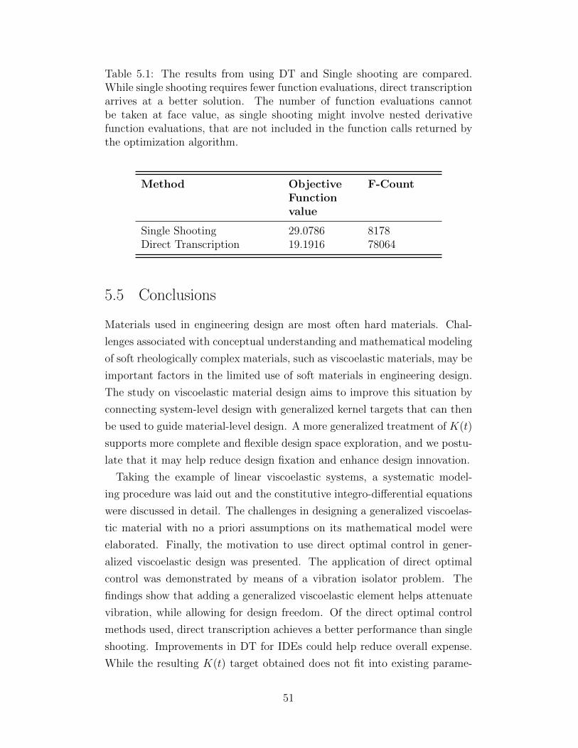
Table 5.1: The results from using DT and Single shooting are compared.While single shooting requires fewer function evaluations, direct transcriptionarrives at a better solution. The number of function evaluations cannotbe taken at face value, as single shooting might involve nested derivativefunction evaluations, that are not included in the function calls returned bythe optimization algorithm.

Method ObjectiveFunctionvalue

F-Count

Single Shooting 29.0786 8178Direct Transcription 19.1916 78064

5.5 Conclusions

Materials used in engineering design are most often hard materials. Chal-

lenges associated with conceptual understanding and mathematical modeling

of soft rheologically complex materials, such as viscoelastic materials, may be

important factors in the limited use of soft materials in engineering design.

The study on viscoelastic material design aims to improve this situation by

connecting system-level design with generalized kernel targets that can then

be used to guide material-level design. A more generalized treatment of K(t)

supports more complete and flexible design space exploration, and we postu-

late that it may help reduce design fixation and enhance design innovation.

Taking the example of linear viscoelastic systems, a systematic model-

ing procedure was laid out and the constitutive integro-differential equations

were discussed in detail. The challenges in designing a generalized viscoelas-

tic material with no a priori assumptions on its mathematical model were

elaborated. Finally, the motivation to use direct optimal control in gener-

alized viscoelastic design was presented. The application of direct optimal

control was demonstrated by means of a vibration isolator problem. The

findings show that adding a generalized viscoelastic element helps attenuate

vibration, while allowing for design freedom. Of the direct optimal control

methods used, direct transcription achieves a better performance than single

shooting. Improvements in DT for IDEs could help reduce overall expense.

While the resulting K(t) target obtained does not fit into existing parame-

51

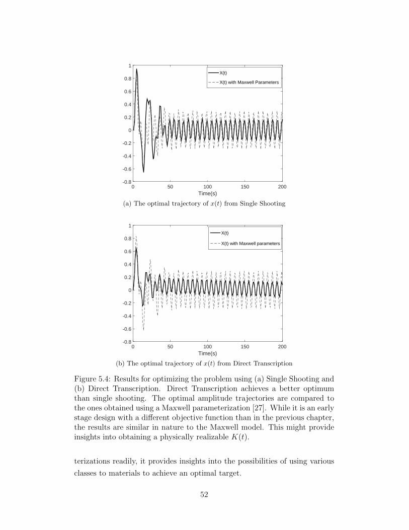
Time(s)0 50 100 150 200

-0.8

-0.6

-0.4

-0.2

0

0.2

0.4

0.6

0.8

1X(t)

X(t) with Maxwell Parameters

(a) The optimal trajectory of x(t) from Single Shooting

Time(s)0 50 100 150 200

-0.8

-0.6

-0.4

-0.2

0

0.2

0.4

0.6

0.8

1X(t)

X(t) with Maxwell parameters

(b) The optimal trajectory of x(t) from Direct Transcription

Figure 5.4: Results for optimizing the problem using (a) Single Shooting and(b) Direct Transcription. Direct Transcription achieves a better optimumthan single shooting. The optimal amplitude trajectories are compared tothe ones obtained using a Maxwell parameterization [27]. While it is an earlystage design with a different objective function than in the previous chapter,the results are similar in nature to the Maxwell model. This might provideinsights into obtaining a physically realizable K(t).

terizations readily, it provides insights into the possibilities of using various

classes to materials to achieve an optimal target.

52

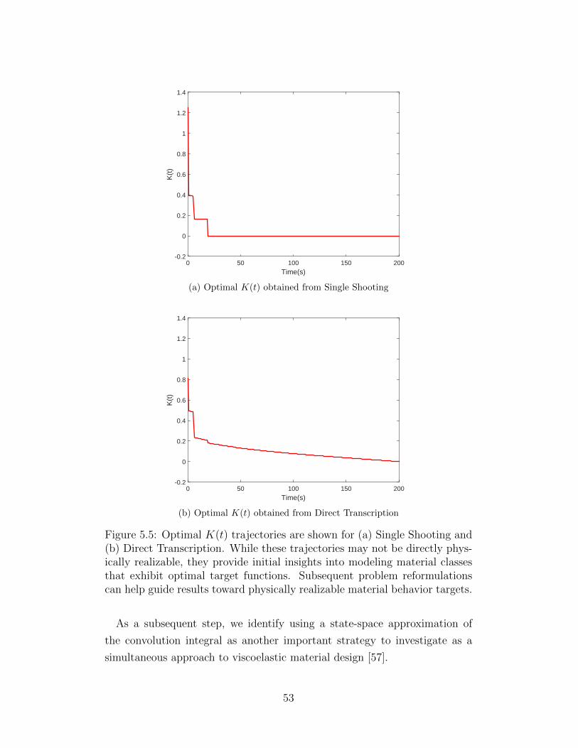
Time(s)0 50 100 150 200

K(t

)

-0.2

0

0.2

0.4

0.6

0.8

1

1.2

1.4

(a) Optimal K(t) obtained from Single Shooting

Time(s)0 50 100 150 200

K(t

)

-0.2

0

0.2

0.4

0.6

0.8

1

1.2

1.4

(b) Optimal K(t) obtained from Direct Transcription

Figure 5.5: Optimal K(t) trajectories are shown for (a) Single Shooting and(b) Direct Transcription. While these trajectories may not be directly phys-ically realizable, they provide initial insights into modeling material classesthat exhibit optimal target functions. Subsequent problem reformulationscan help guide results toward physically realizable material behavior targets.

As a subsequent step, we identify using a state-space approximation of

the convolution integral as another important strategy to investigate as a

simultaneous approach to viscoelastic material design [57].

53

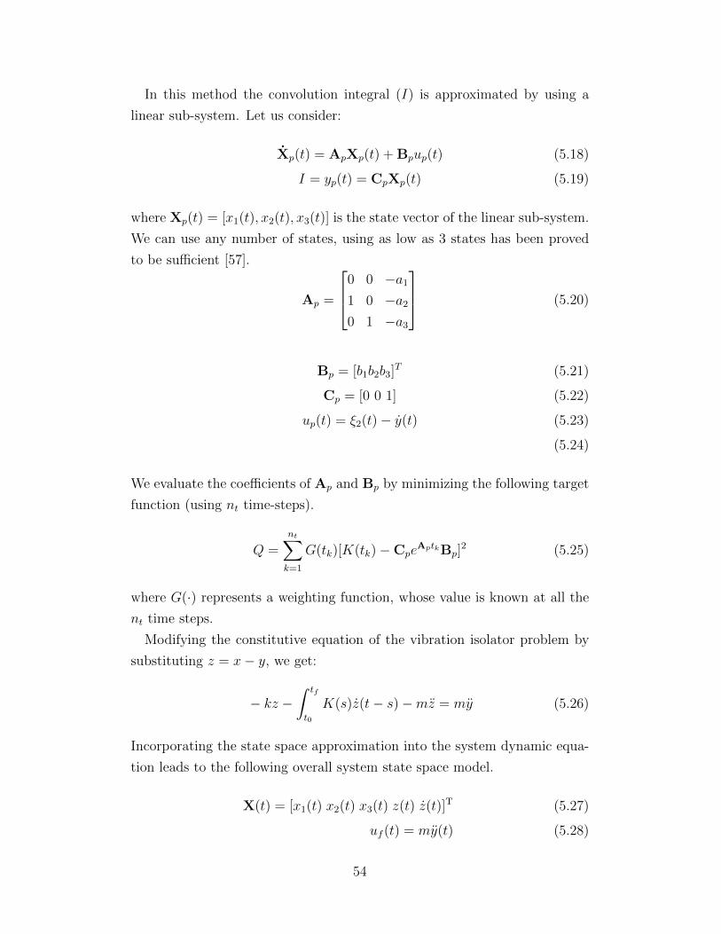
In this method the convolution integral (I) is approximated by using a

linear sub-system. Let us consider:

Xp(t) = ApXp(t) + Bpup(t) (5.18)

I = yp(t) = CpXp(t) (5.19)

where Xp(t) = [x1(t), x2(t), x3(t)] is the state vector of the linear sub-system.

We can use any number of states, using as low as 3 states has been proved

to be sufficient [57].

Ap =

0 0 −a11 0 −a20 1 −a3

(5.20)

Bp = [b1b2b3]T (5.21)

Cp = [0 0 1] (5.22)

up(t) = ξ2(t)− y(t) (5.23)

(5.24)

We evaluate the coefficients of Ap and Bp by minimizing the following target

function (using nt time-steps).

Q =nt∑

k=1

G(tk)[K(tk)−CpeAptkBp]

2 (5.25)

where G(·) represents a weighting function, whose value is known at all the

nt time steps.

Modifying the constitutive equation of the vibration isolator problem by

substituting z = x− y, we get:

− kz −∫ tf

t0

K(s)z(t− s)−mz = my (5.26)

Incorporating the state space approximation into the system dynamic equa-

tion leads to the following overall system state space model.

X(t) = [x1(t) x2(t) x3(t) z(t) z(t)]T (5.27)

uf (t) = my(t) (5.28)

54

The state space matrices are given by:

A =

0 0 −a1 0 b1

1 0 −a2 0 b2

0 1 −a3 0 b3

0 0 0 0 1

0 0 −1/m −k/m 0

(5.29)

B = [0 0 0 0 − 1/m] (5.30)

C = [0 0 0 1 0]T (5.31)

Thus, the simultaneous formulation can be expressed as:

minΞ,K,Ap,Bp

∫ tf

t0

|z|

subject to X(t0) = 0

dK(t)

dt≤ 0

ζ(X(t),K) = 0

Q =nt∑

k=1

G(tk)[K(tk)−CpeAptkBp]

2 ≤ ε

(5.32)

where ζ(X(t),K) = X(t)−AX(t)−Buf and ε is a chosen tolerance value.

Cumulatively, a benchmarking of the the numerical methods with respect

to efficiency and convergence would be required. The other crucial part

in our future exploration is to understand the physical realizations of the

optimal target K(t). By understanding the relationship between the target

and physically feasible materials, we can potentially go on to create a better

mathematical model of a generalized viscoelastic system.

55

CHAPTER 6

Adaptive Surrogate Modelingbased Multi-Objective Optimization

Many engineering applications involve multiple design objectives, typically

centered on enhancing performance and reducing cost. Apart from hav-

ing multiple design goals, engineering systems are also usually characterized

by computationally intensive simulations. Despite advances in computing

power in the recent past, computationally intensive analysis methods (e.g.,

Computational Fluid Dynamics (CFD)) can be impractical to use with op-

timization directly [2]. Important fluid power system design objectives, such

as friction across sliding contacts, often require an expensive CFD simulation

of the Navier-Stokes equation for each new design candidate. One effective

strategy for reducing the total number of high-fidelity simulations required

to solve a design optimization problem is optimize using an approximate

surrogate model (SM)—sometimes called a meta-model—of the high-fidelity

model [64, 65]. Accurate solution requires acceptable SM accuracy in the

neighborhood of the optimum. Adaptive surrogate modeling methods itera-

tively assess SM accuracy, and evaluate the high-fidelity model at new sample

points to improve SM accuracy if needed in strategic regions of the design

space [66, 67]. The cost of evaluating sample points using the high-fidelity

model must be accounted for when comparing SM to direct optimization.

SM has been investigated for specific application domains, such as struc-

tural design [68] and injection molding [69]. While most studies have focused

on single-objective problems (e.g., Ref. [70]), extensions of SM to MOO have

been made [69]. This chapter presents advancements of adaptive SM for

MOO that aim to reduce the number of required simulations further. New

features of this method include enforcement of constraints during high-fidelity

model sampling. The algorithmic approach is elucidated using a mathemat-

ical example, followed by a physical engineering application that employs a

CFD simulation of Newtonian fluids on microtextures.

56

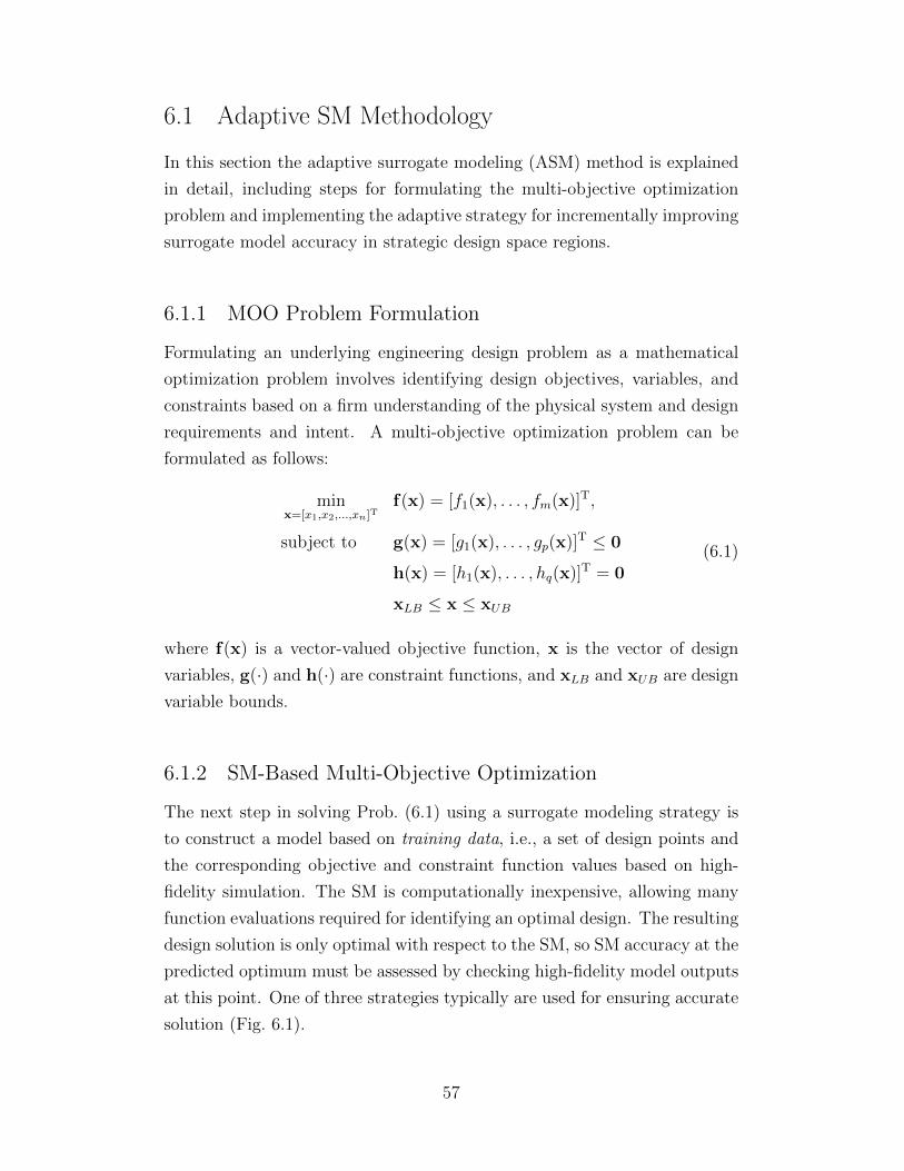
6.1 Adaptive SM Methodology

In this section the adaptive surrogate modeling (ASM) method is explained

in detail, including steps for formulating the multi-objective optimization

problem and implementing the adaptive strategy for incrementally improving

surrogate model accuracy in strategic design space regions.

6.1.1 MOO Problem Formulation

Formulating an underlying engineering design problem as a mathematical

optimization problem involves identifying design objectives, variables, and

constraints based on a firm understanding of the physical system and design

requirements and intent. A multi-objective optimization problem can be

formulated as follows:

minx=[x1,x2,...,xn]T

f(x) = [f1(x), . . . , fm(x)]T,

subject to g(x) = [g1(x), . . . , gp(x)]T ≤ 0

h(x) = [h1(x), . . . , hq(x)]T = 0

xLB ≤ x ≤ xUB

(6.1)

where f(x) is a vector-valued objective function, x is the vector of design

variables, g(·) and h(·) are constraint functions, and xLB and xUB are design

variable bounds.

6.1.2 SM-Based Multi-Objective Optimization

The next step in solving Prob. (6.1) using a surrogate modeling strategy is

to construct a model based on training data, i.e., a set of design points and

the corresponding objective and constraint function values based on high-

fidelity simulation. The SM is computationally inexpensive, allowing many

function evaluations required for identifying an optimal design. The resulting

design solution is only optimal with respect to the SM, so SM accuracy at the

predicted optimum must be assessed by checking high-fidelity model outputs

at this point. One of three strategies typically are used for ensuring accurate

solution (Fig. 6.1).

57

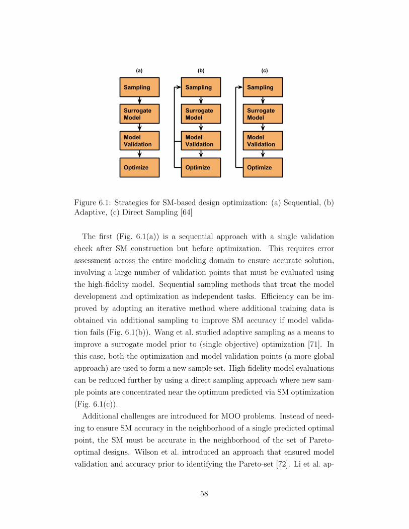
Sampling

Surrogate Model

Model Validation

Optimize

Sampling

Surrogate Model

Model Validation

Optimize

Sampling

Surrogate Model

Model Validation

Optimize

(a) (b) (c)

Figure 6.1: Strategies for SM-based design optimization: (a) Sequential, (b)Adaptive, (c) Direct Sampling [64]

The first (Fig. 6.1(a)) is a sequential approach with a single validation

check after SM construction but before optimization. This requires error

assessment across the entire modeling domain to ensure accurate solution,

involving a large number of validation points that must be evaluated using

the high-fidelity model. Sequential sampling methods that treat the model

development and optimization as independent tasks. Efficiency can be im-

proved by adopting an iterative method where additional training data is

obtained via additional sampling to improve SM accuracy if model valida-

tion fails (Fig. 6.1(b)). Wang et al. studied adaptive sampling as a means to

improve a surrogate model prior to (single objective) optimization [71]. In

this case, both the optimization and model validation points (a more global

approach) are used to form a new sample set. High-fidelity model evaluations

can be reduced further by using a direct sampling approach where new sam-

ple points are concentrated near the optimum predicted via SM optimization

(Fig. 6.1(c)).

Additional challenges are introduced for MOO problems. Instead of need-

ing to ensure SM accuracy in the neighborhood of a single predicted optimal

point, the SM must be accurate in the neighborhood of the set of Pareto-

optimal designs. Wilson et al. introduced an approach that ensured model

validation and accuracy prior to identifying the Pareto-set [72]. Li et al. ap-

58

proximated Pareto sets using a hyper-ellipse [73]. Shan and Wang developed

a new method—Pareto-Set Pursuing (PSP)—that addresses the challenges

of solving MOO problems based on computationally expensive models [74].

The Adaptive Surrogate Modeling method for Multi-Objective Optimiza-

tion (ASM-MOO) methodology presented here is a direct sampling approach.

The case study involves a challenging fluid-flow system design problem, but

the methodology can be extended to a general class of design problems. We

introduce design constraint enforcement at the sampling stage, and study

the resulting efficiency of this modified sampling method.

6.2 ASM-MOO Algorithm Framework

A more detailed illustration of the ASM-MOO methodology is shown in

Fig. 6.2. The modeling domain Dm is the region of the design space over

which the SM is constructed. This may be fixed, or may contract and shift

to conserve modeling efforts. The superscript k is the iteration counter. The

sampling domain Ds is the design space region over which new sample points

are defined; design sample points and their corresponding simulation outputs

are used for the training dataset T .

During initialization the sampling domain Ds is defined to be the same

as the modeling domain, as no information is available yet to help focus

sampling efforts near the predicted Pareto-optimal points. It is desirable to

avoid using sample points that violate design constraints for two reasons: 1)

Often infeasible points cannot be simulated [75], and 2) even if simulation

is possible, simulation of infeasible points is wasted effort as SM accuracy

is unimportant in infeasible regions. Here a set of preliminary samples are

generated using one of several appropriate space-filling sampling techniques

(such as Latin Hypercube) in the preliminary sampling domain Ds. This

domain may include infeasible points. This set of sample points is then

filtered to remove infeasible points, i.e., retained sample points belong to the

set Ds = Ds ∈ F , where F is the feasible domain (i.e., the set of points that

satisfy design constraints). In the studies presented here design constraints

are analytical, so SMs for design constraints are not needed.

T is then formed by evaluating each retained sample point using the high-

fidelity model, and organizing these data pairs. The SM is then constructed

59

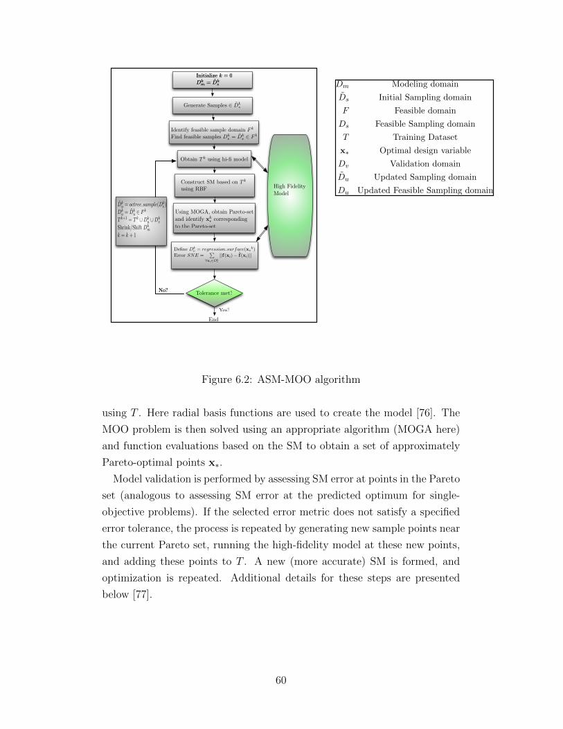
Dm Modeling domain

Ds Initial Sampling domain

F Feasible domain

Ds Feasible Sampling domain

T Training Dataset

x∗ Optimal design variable

Dv Validation domain

Du Updated Sampling domain

Du Updated Feasible Sampling domain

Initialize k = 0Dk

m = Dks

Initialize k = 0Dk

m = Dks

Generate Samples 2 Dks

Construct SM based on T k

using RBF

Using MOGA, obtain Pareto-setand identify xk

⇤ correspondingto the Pareto-set

Define Dkv = regression surface(x⇤k)

Error SNE =P

8xi2Dkv

||f(xi) � f(xi)||

Tolerance met?

High FidelityModel

No?No?

Yes?

End

Dku = octree sample(Dk

v )Dk

u = Dku 2 F k

T k+1 = T k [ Dku [ Dk

v

Shrink/Shift Dkm

k = k + 1

Identify feasible sample domain F k

Find feasible samples Dks = Dk

s 2 F k

Obtain T k using hi-fi model

Figure 6.2: ASM-MOO algorithm

using T . Here radial basis functions are used to create the model [76]. The

MOO problem is then solved using an appropriate algorithm (MOGA here)

and function evaluations based on the SM to obtain a set of approximately

Pareto-optimal points x∗.

Model validation is performed by assessing SM error at points in the Pareto

set (analogous to assessing SM error at the predicted optimum for single-

objective problems). If the selected error metric does not satisfy a specified

error tolerance, the process is repeated by generating new sample points near

the current Pareto set, running the high-fidelity model at these new points,

and adding these points to T . A new (more accurate) SM is formed, and

optimization is repeated. Additional details for these steps are presented

below [77].

60

6.2.1 Sampling

The modeling domain Dm is defined here by the design variable bounds.

Due to the SM type and the nature of the case studies, Dm was not adjusted

during the the ASM-MOO process. Here Ds = Dm, and a suitable design of

experiments (DOE) technique is used to generate sample points that lie in

Ds. The appropriate choice of sampling technique depend on factors such as

(i) design space dimension, (ii) estimated level of response noise, and (iii) SM

type. For noisy data (e.g., probabilistic models), DOEs that reduce the sensi-

tivity to noise are desirable, such as central composite designs, face-centered

cubic designs, factorial designs, and Box-Behnken designs [78]. For systems

with less noise (such as deterministic models), Latin-Hypercube Sampling

(LHS), minimum bias designs, and Orthogonal Arrays (OAs) are preferred.

Here LHS is used, which is an example of a space-filling design that is of-

ten effective for computer experiments without variance [79–81], including

adaptive surrogate modeling [82] and in conjunction with OAs [83].

6.2.2 Filtering Infeasible Sampling Points

Engineering design problems often involve inequality constraints g(·) ≤ 0.

The sampling procedure described above ensures that only feasible design

points are evaluated using the high-fidelity model, improving overall effi-

ciency. In some cases this strategy offers another important advantage: sam-

ple points that violate constraints may not be physically meaningful, or for

other reasons would cause simulation failure. Removing infeasible preemp-

tively avoids these simulation problems that are otherwise difficult to manage

in an optimization implementation [75]. We investigate how filtering out in-

feasible sample points influences solution efficiency.

While this algorithm addresses only analytically defined linear and non-

linear constraints, we acknowledge the need to extend this study to con-

straints that require the simulation of the high-fidelity model. Filtering out

infeasible points based on approximated constraint functions is an impor-

tant topic for future work. It is expected that additional challenges will be

encountered as there is uncertainty in whether sample points are actually

infeasible during the ASM solution process.

61

6.2.3 Surrogate Model Construction

Once the set of feasible sample points is defined, these design points are evalu-

ated using the high-fidelity model. This produces input-output pairs that are

added to the set of training data T to be used for SM construction. A wide

variety of approximation function types may be used for SM construction.

Several general-purpose options are described below. Application-specific

SMs may help improve solution efficiency further.

General purpose approximation functions for SMs help to estimate simu-

lation output at design points other than those in T . Well-known options

include Kriging [81, 84], artificial neural networks (ANNs) [85], and radial

basis functions [86,87]. Other methods include multivariate adaptive regres-

sion splines (MARS) [88], least interpolating polynomials [89], and inductive

learning [90]. Jin et al. compared several different surrogate models and

concluded that the appropriate model choice depends on the degree of sys-

tem nonlinearity [91]. Stander et al. compared polynomial response surface

approximation, Kriging, and neural networks [92], and discovered that while

neural networks and Kriging models require a larger number of initial points,

their algorithmic efficiencies are comparable to a polynomial model. The gen-

eral conclusion from the literature demonstrates that there is no single best

SM type that satisfies all problems. Haftka et al. address this issue by explor-

ing the use of an ensemble or a weighted average SM in place of individual

surrogates [93]. The best model choice depends on the nature of the problem

and the sampled data set.

Radial basis functions have been used extensively as SMs for engineering

design optimization [76, 94]. Fang et al. compared polynomial response and

radial basis functions and found that RBFs are more effective at handling

non-linearities in some cases [95]. RBF models have been selected for use in

this article. Comparison with other model types is an important topic for

future work.

When using an RBF approximation for multi-objective problems, an ap-

proximate function is defined for each of the m objective function values.

As part of this definition, the interpolation condition for the jth objective

function is formulated using ns training points:

62

fj(xi) =ns∑

k=1

wjkψ(||xi − ck||), i = 1, 2 . . . ns

j = 1, 2 . . .m

(6.2)

where ψ(.) is the radial basis function, wjk are unknown weighting coeffi-

cients, xi is the ith training point, and ck is the kth basis function center.

The RBF used here is the thin plate spline function [96]: ψ(r) = r2 ln r,

where r is the Euclidean distance between the training point and function

center: r = (||xi − ck||).During SM construction we seek to find the coefficients wji that solve

ψwj = fj, where ψi,k = ψ(||xi − ck||), i, k = 1, 2 . . . ns is the Gram ma-

trix, and the vector of training outputs for the jth objective function is

fj = [fj(x1), fj(x2), . . . , fj(xns)]T [96]. This equation has a unique solution

since the Gram matrix is square. To reduce problem complexity here we

assume that the RBF centers coincide with training points, i.e., ci = xi.

Once the coefficients wjk are identified for each objective function the ap-

proximate objective functions can be defined: f(x) = [f1(x), . . . , fm(x)]T.

For a given point in the design space x, we can compute the row vector

ψ(x) = [ψ(||x − c1||), . . . , ψ(||x − cns||)]. The surrogate model for the jth

objective function is fj(x) = ψ(x)wj.

6.2.4 Surrogate Model Optimization

The multi-objective design optimization problem is then solved by replacing

the original nonlinear functions in Prob. (6.1) with approximate functions

obtained via surrogate modeling. This produces an approximate Pareto set

that is only accepted as the solution if the validation step is passed. If all

objective and constraint functions are approximated using surrogates, the

updated problem formulation is:

minx=[x1,x2,...,xn]T

f(x) = [f1(x), . . . , fm(x)]T,

subject to g(x) = [g1(x), . . . , gp(x)]T ≤ 0

h(x) = [h1(x), . . . , hq(x)]T = 0

xLB ≤ x ≤ xUB

(6.3)

63

The solution of a MOO problem involves a set of solutions, known as the

Pareto-optimal set (or Pareto set), that consists of non-dominated optimal

points and quantifies design trade-offs in the objective function space. Many

strategies exist for addressing MOO design problems [97, 98], some of which

include condensing the multiple objectives into a single objective function by

using a weighted sum or a geometric mean. An alternative treats all but one

objective as a constraint. In either case multiple optimization solutions are

required to build up the Pareto set, each time varying objective weights or

constraint bounds. Another class of MOO solution methods are evolutionary

algorithms such as the Multi-Objective Genetic Algorithm (MOGA) and

the Non-dominated Sorting Genetic Algorithm (NSGA-II) [99, 100], both of

which produce multiple Pareto-optimal solutions in a single optimization

execution.

This MOO problem was solved here using a Multi-Objective Genetic Al-

gorithm (MOGA), a specific class of evolutionary algorithms [101]. The pri-

mary advantage of evolutionary algorithms for MOO is that an approximate

Pareto set can be generated via a single MOGA solution.

6.2.5 Surrogate Model Validation

Surrogate models used in design optimization need to be accurate in the

region of the optimum. Guaranteeing accuracy within a tolerance at other

points in the design points is wasteful of resources. Validation is straightfor-

ward for single objective problems where SM accuracy must be verified near

the single predicted optimal point. This can be accomplished by evaluating

the high-fidelity model at the predicted optimum, and comparing the result

to the SM output at this point. SM validation is more involved for MOO

problems. We need to ensure that the SM is accurate for points in the de-

sign space that are Pareto-optimal. Instead of validating the SM at a single

point, it must be validated across a bounded hypersurface. For this purpose

we define the validation domain Dv to be the set of points over which the

SM must be validated. If the design space is in Rn, the hypersurface that

defines Dv is a manifold of dimension n− 1.

Validating over bounded hypersurface introduces two core challenges: 1)

Instead of validating a single point in the design space, validation must be

64

performed across an infinite number of points on a hypersurface, and 2) The

boundaries of this hypersurface may be complicated (possibly non-convex or

even disconnected), and we should focus validation efforts on points within

the hypersurface bounds. The first challenge is addressed by using regression

to fit a surface through Pareto-optimal points in the design space to define an

approximate (unbounded) validation domain. A uniform sampling technique

is then used to select a finite set of validation points from Dv for validation.

Generating these new validation points in Dv is required because simply

using the Pareto-optimal points identified by the MOGA as validation points

may not be adequate due to non-uniform distribution in the design space.

The error between the SM and the high-fidelity model is evaluated at these

validation points, and these error quantities are combined into a single error

metric for SM validation.

In addressing the second challenge we recognize that not every point on

an unbounded regression surface that is fit through Pareto-optimal points is

in the Pareto set. We must identify and stay within hypersurface bounds to

ensure that validation points are (approximately) in the Pareto set.

Several options exist for defining the validation hypersurface Dv, includ-

ing simple regression, non-uniform rational basis splines (NURBS) [102], or

T-splines. Quadratic regression performed well for the small-dimension case

studies used here. Support Vector Data Description (SVDD) could be used

to define a precise hypersurface boundary that includes all known Pareto-

optimal points [75, 103]. Rather than defining a precise boundary, we devel-

oped an algorithm that generated random points on the hypersurface that

were within a convex hull of a subset of the known Pareto-optimal points.

This provided an efficient means of generating validation points that were

approximately in the true Dv.

Once validation points are chosen, the high-fidelity model is evaluated

at these points for comparison to the SM to evaluate accuracy. Several

options for SM validation exist, but standard methods are intended primarily

for cases where accuracy is being assessed across Dm. Cross-validation is a

popular method used for this purpose. It involves starting with a dataset,

X, Y consisting of n input-output data pairs (x, y), where y is the high-fidelity

model response at the design sample point, x, and ns is the total number

of function evaluations used for combined training and validation. In p-fold

cross validation, the initial validation data set is split into p different subsets.

65

The metamodel is then fit p times, each time leaving out one of the subsets

from training, and using the omitted subset for validation. Since this is

computationally cumbersome, Meckesheimer [104,105] suggested a leave-one

out cross-validation strategy, applicable to radial basis functions.

The method used here is to evaluate the standard normal error (SNE) using

points in Dv. For a set of nv validation points, the norm of the difference

between the actual function value and the approximated function value is

defined as the SNE:

SNE =nv∑

i=1

||(f(xi)− f(xi))|| (6.4)

where xi is the design vector value for the ith validation point.

6.2.6 Sampling Domain Update

If the SNE ≥ εv, where εv is a specified validation tolerance, model accuracy

must be improved in the neighborhood of the Pareto set. This is done by

generating new sample points that are in Du, which is the updated sampling

domain that includes a small neighborhood of the design space near Dv. The

high-fidelity model is evaluated at these new sample points, and these data

pairs (along with the validation points from the previous set) are appended

to T for use in constructing the updated SM with improved accuracy near

the estimated Pareto set.

Sample points need to be defined that lie within Du, which is a hypervol-

ume. One approach would be to define the boundary of this hypervolume

directly (using SVDD, level set methods, etc.) and filter out sample points

that are not within this boundary. A classification method such as a Sup-

port Vector Machine (SVM) could be used to determine whether candidate

sample points are within Du [103, 106]. Alternatively, force-directed layout

or field functions could be used to increase the density of sample points near

Dv.

The method used here is an Octree-based sampling method [107] that gen-

erates uniformly distributed points in the neighborhood of validation points

as shown in Fig. 6.3. Sample point density can be adjusted as the ASM-MOO

algorithm progresses. Given a specified distance tolerance, points lying far

66

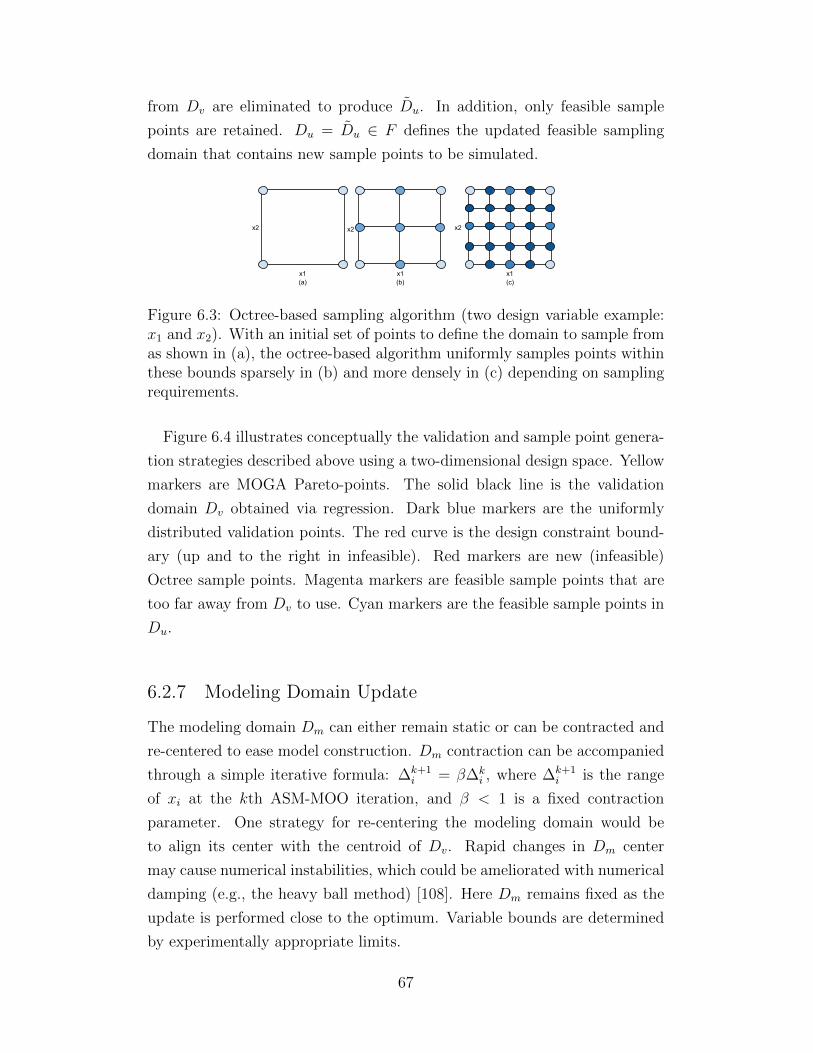
from Dv are eliminated to produce Du. In addition, only feasible sample

points are retained. Du = Du ∈ F defines the updated feasible sampling

domain that contains new sample points to be simulated.

x1 x1 x1

x2 x2 x2

(a) (b) (c)

Figure 6.3: Octree-based sampling algorithm (two design variable example:x1 and x2). With an initial set of points to define the domain to sample fromas shown in (a), the octree-based algorithm uniformly samples points withinthese bounds sparsely in (b) and more densely in (c) depending on samplingrequirements.

Figure 6.4 illustrates conceptually the validation and sample point genera-

tion strategies described above using a two-dimensional design space. Yellow

markers are MOGA Pareto-points. The solid black line is the validation

domain Dv obtained via regression. Dark blue markers are the uniformly

distributed validation points. The red curve is the design constraint bound-

ary (up and to the right in infeasible). Red markers are new (infeasible)

Octree sample points. Magenta markers are feasible sample points that are

too far away from Dv to use. Cyan markers are the feasible sample points in

Du.

6.2.7 Modeling Domain Update

The modeling domain Dm can either remain static or can be contracted and

re-centered to ease model construction. Dm contraction can be accompanied

through a simple iterative formula: ∆k+1i = β∆k

i , where ∆k+1i is the range

of xi at the kth ASM-MOO iteration, and β < 1 is a fixed contraction

parameter. One strategy for re-centering the modeling domain would be

to align its center with the centroid of Dv. Rapid changes in Dm center

may cause numerical instabilities, which could be ameliorated with numerical

damping (e.g., the heavy ball method) [108]. Here Dm remains fixed as the

update is performed close to the optimum. Variable bounds are determined

by experimentally appropriate limits.

67

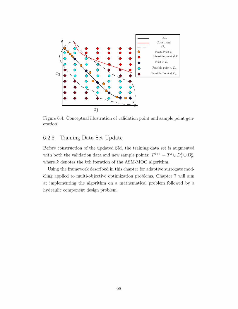
Dv

ConstraintDu

Feasible point 2 Du

Infeasible point /2 F

Feasible Point /2 Du

Point in Dv

x1

x2

Pareto Point x⇤

Figure 6.4: Conceptual illustration of validation point and sample point gen-eration

6.2.8 Training Data Set Update

Before construction of the updated SM, the training data set is augmented

with both the validation data and new sample points: T k+1 = T k ∪Dku ∪Dk

v ,

where k denotes the kth iteration of the ASM-MOO algorithm.

Using the framework described in this chapter for adaptive surrogate mod-

eling applied to multi-objective optimization problems, Chapter 7 will aim

at implementing the algorithm on a mathematical problem followed by a

hydraulic component design problem.

68

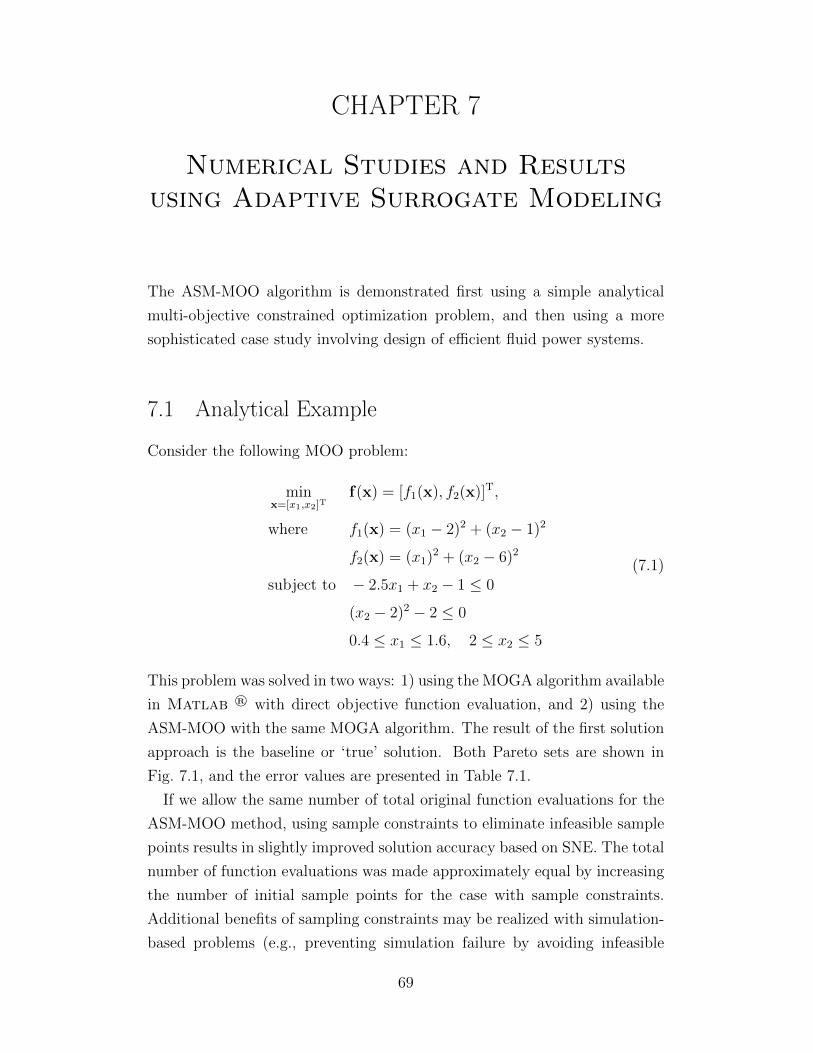
CHAPTER 7

Numerical Studies and Resultsusing Adaptive Surrogate Modeling

The ASM-MOO algorithm is demonstrated first using a simple analytical

multi-objective constrained optimization problem, and then using a more

sophisticated case study involving design of efficient fluid power systems.

7.1 Analytical Example

Consider the following MOO problem:

minx=[x1,x2]T

f(x) = [f1(x), f2(x)]T,

where f1(x) = (x1 − 2)2 + (x2 − 1)2

f2(x) = (x1)2 + (x2 − 6)2

subject to − 2.5x1 + x2 − 1 ≤ 0

(x2 − 2)2 − 2 ≤ 0

0.4 ≤ x1 ≤ 1.6, 2 ≤ x2 ≤ 5

(7.1)

This problem was solved in two ways: 1) using the MOGA algorithm available

in Matlab ® with direct objective function evaluation, and 2) using the

ASM-MOO with the same MOGA algorithm. The result of the first solution

approach is the baseline or ‘true’ solution. Both Pareto sets are shown in

Fig. 7.1, and the error values are presented in Table 7.1.

If we allow the same number of total original function evaluations for the

ASM-MOO method, using sample constraints to eliminate infeasible sample

points results in slightly improved solution accuracy based on SNE. The total

number of function evaluations was made approximately equal by increasing

the number of initial sample points for the case with sample constraints.

Additional benefits of sampling constraints may be realized with simulation-

based problems (e.g., preventing simulation failure by avoiding infeasible

69

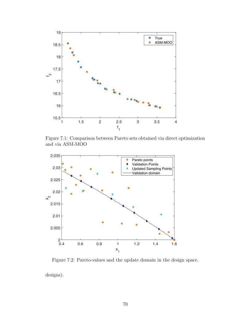
f11 1.5 2 2.5 3 3.5 4

f 2

15.5

16

16.5

17

17.5

18

18.5

19TrueASM-MOO

Figure 7.1: Comparison between Pareto sets obtained via direct optimizationand via ASM-MOO

x1

0.4 0.6 0.8 1 1.2 1.4 1.6

x 2

2

2.005

2.01

2.015

2.02

2.025

2.03

2.035Pareto pointsValidation PointsUpdated Sampling PointsValidation domain

Figure 7.2: Pareto-values and the update domain in the design space.

designs).

70

Table 7.1: Results from using sampling constraints on the analytical example.In each case the methods used approximately the samenumber of original function evaluations.

Method No. of iter-ations

SNE

ASM-MOO w/o sam-pling constraints

8 8.26e-04

ASM-MOO with sam-pling constraints

6 6.20e-04

7.2 Design for Efficient Fluid Power

A hydraulic system design study motivated the development of the ASM-

MOO method introduced in this article. This study involves the investiga-

tion of different surface texture designs for components used in fluid power

systems where metal parts are in sliding contact separated by hydraulic fluid.

The competing design objectives investigated here include reducing effective

viscosity (related to friction) and the cross-sectional area of the texture (re-

lated to cost).

Previous studies have shown that the use of surface textures aids in de-

creasing friction in lubricated sliding contact [109]. Schuh and Ewoldt [110]

have experimentally examined the effects of using symmetric and asymmet-

ric textures to decrease viscous friction and increase normal force production

with Newtonian lubricants. For the experiments, a DHR-3 gap controlled

rotational rheometer was used with the textured plates mounted to a tem-

perature controlled Peltier plate with Crystalbond, a thermo-reversible ad-

hesive. A schematic of the experimental set up is given in Fig. 7.3, and the

measured geometric properties of the textures tested are given in Fig. ??.

In their experiments, Schuh and Ewoldt found that symmetric textures

decreased the viscous friction more than the asymmetric textures, but the

asymmetric textures produced larger normal forces than the symmetric ones

(important for sealing).

Since each texture profile met both of the given design objectives, but met

them to differing degrees, this presents an interesting opportunity to study

optimal tradeoffs for texture profile design. A computer experiment of the

71

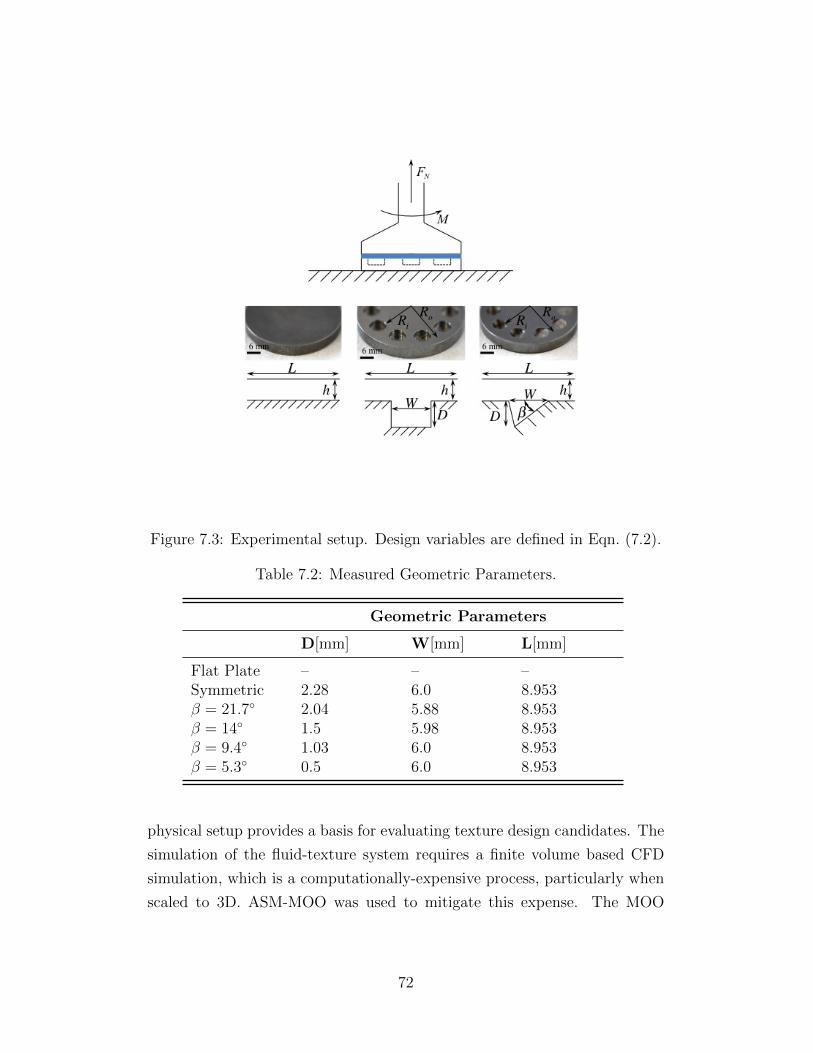
Figure 7.3: Experimental setup. Design variables are defined in Eqn. (7.2).

Table 7.2: Measured Geometric Parameters.

Geometric Parameters

D[mm] W[mm] L[mm]

Flat Plate – – –Symmetric 2.28 6.0 8.953β = 21.7◦ 2.04 5.88 8.953β = 14◦ 1.5 5.98 8.953β = 9.4◦ 1.03 6.0 8.953β = 5.3◦ 0.5 6.0 8.953

physical setup provides a basis for evaluating texture design candidates. The

simulation of the fluid-texture system requires a finite volume based CFD

simulation, which is a computationally-expensive process, particularly when

scaled to 3D. ASM-MOO was used to mitigate this expense. The MOO

72

problem for this case study is defined as follows:

minx=[x1,x2,x3]T

f(x) = [f1(x), f2(x)]T, (7.2a)

where f1 = ηa/η0 (7.2b)

f2 = x1x2 (7.2c)

x1 = Texture width: W (mm) (7.2d)

x2 = Texture depth: D (mm) (7.2e)

x3 = Plate length: L (mm) (7.2f)

subject to x2 ≤ 0.95x4, (7.2g)

0 ≤ x1 ≤ 6 (7.2i)

0 ≤ x2 ≤ 2 (7.2j)

0.8953 ≤ x3 ≤ 8.953 (7.2k)

Training data was obtained via FLUENT, a finite volume-based CFD solver.

Symmetric and asymmetric texture profiles were simulated at steady state

in FLUENT using a Newtonian lubricant with a viscosity of 0.140 Pa s and

a density of 866.8 kg/m3. The simulations were performed using double

precision and parallel computing with two processes. The pressure was solved

using the SIMPLE algorithm and the momentum was solved using the second

order upwind technique. A hybrid initialization scheme was used, and the

simulation was run until all the residuals for the system were less than 1 ×10−5. h was fixed at 0.25 mm. Several different values of W , D, and L were

simulated in order to examine different texture profiles. The results from

FLUENT were given as a normal force and viscous force, and the viscous

force was converted to an apparent viscosity using:

ηa =Fv

WLUh

(7.3)

where U is the velocity of the top plate, which for these simulations was set

as U = 1.425m/s.

The design constraint x1 ≤ 0.95x3 ensures that texture width is no greater

than 95% of the length of the moving plate. The simulation would be in-

feasible (or produce insensible output) if the constraint is violated. RBFs

73

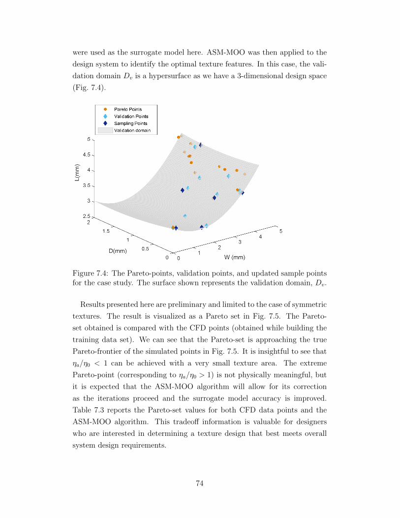
were used as the surrogate model here. ASM-MOO was then applied to the

design system to identify the optimal texture features. In this case, the vali-

dation domain Dv is a hypersurface as we have a 3-dimensional design space

(Fig. 7.4).

Figure 7.4: The Pareto-points, validation points, and updated sample pointsfor the case study. The surface shown represents the validation domain, Dv.

Results presented here are preliminary and limited to the case of symmetric

textures. The result is visualized as a Pareto set in Fig. 7.5. The Pareto-

set obtained is compared with the CFD points (obtained while building the

training data set). We can see that the Pareto-set is approaching the true

Pareto-frontier of the simulated points in Fig. 7.5. It is insightful to see that

ηa/η0 < 1 can be achieved with a very small texture area. The extreme

Pareto-point (corresponding to ηa/η0 > 1) is not physically meaningful, but

it is expected that the ASM-MOO algorithm will allow for its correction

as the iterations proceed and the surrogate model accuracy is improved.

Table 7.3 reports the Pareto-set values for both CFD data points and the

ASM-MOO algorithm. This tradeoff information is valuable for designers

who are interested in determining a texture design that best meets overall

system design requirements.

74

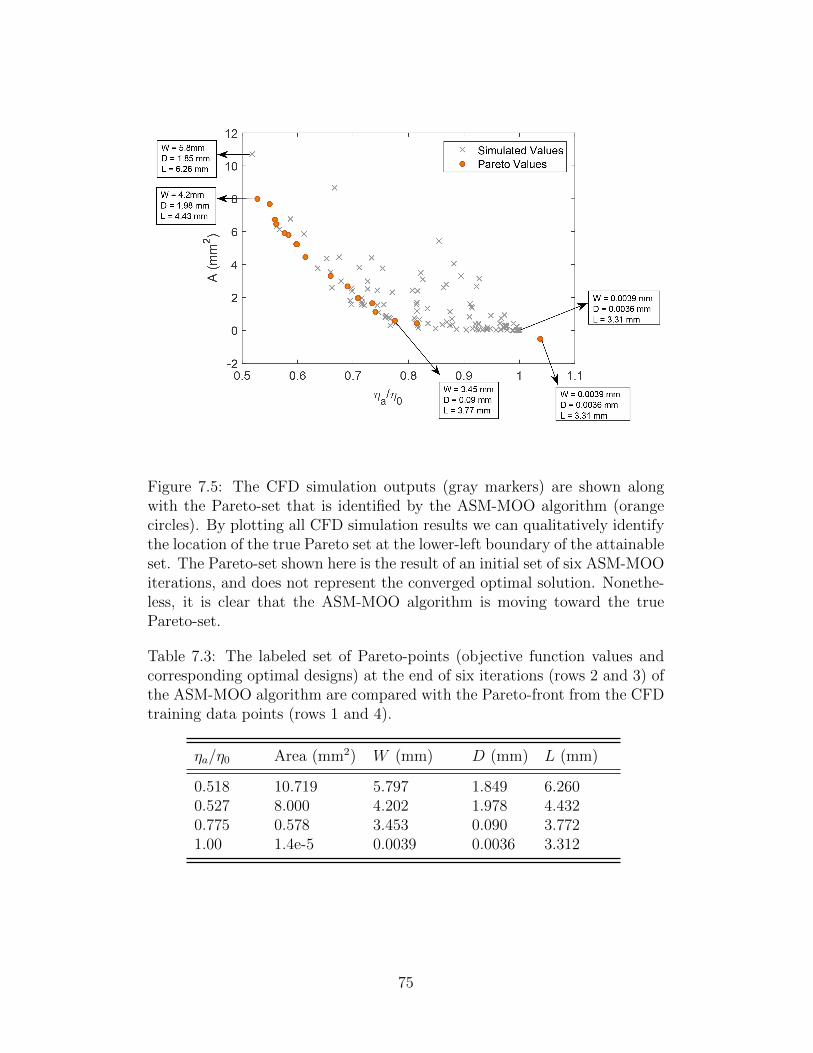
Figure 7.5: The CFD simulation outputs (gray markers) are shown alongwith the Pareto-set that is identified by the ASM-MOO algorithm (orangecircles). By plotting all CFD simulation results we can qualitatively identifythe location of the true Pareto set at the lower-left boundary of the attainableset. The Pareto-set shown here is the result of an initial set of six ASM-MOOiterations, and does not represent the converged optimal solution. Nonethe-less, it is clear that the ASM-MOO algorithm is moving toward the truePareto-set.

Table 7.3: The labeled set of Pareto-points (objective function values andcorresponding optimal designs) at the end of six iterations (rows 2 and 3) ofthe ASM-MOO algorithm are compared with the Pareto-front from the CFDtraining data points (rows 1 and 4).

ηa/η0 Area (mm2) W (mm) D (mm) L (mm)

0.518 10.719 5.797 1.849 6.2600.527 8.000 4.202 1.978 4.4320.775 0.578 3.453 0.090 3.7721.00 1.4e-5 0.0039 0.0036 3.312

75

7.3 Conclusions and Future Work

Engineering design optimization problems are often characterized by multi-

ple objectives and expensive simulations. As a strategy for reducing com-

putational expense, surrogate modeling strategies have been developed and

applied across a variety of engineering domains. In this article, one such

strategy, Adaptive Surrogate Model coupled with Multi-Objective Optimiza-

tion (ASM-MOO), was presented. A systematic formulation of the multi-

objective problem and a detailed framework for the adaptive surrogate mod-

eling was outlined. This algorithm also incorporated the use of design con-

straints in the sampling phase, which is an essential feature particularly in

modeling systems that cannot be simulated in analytical example and is fur-

ther extended to a fluid power component problem.

Future investigations will involve nonlinear sample constraints and design

constraints evaluated using a SM. Alternative strategies for generating fea-

sible samples should be explored (e.g., mapping a hypercube to F in the

neighborhood of Dv). The case study provides great insights into plausible

mictrotexture geometries for different design needs. However, it is limited

currently to symmetric textures; ongoing work is addressing the case of asym-

metric textures as well. Aside from texture geometry, we envision studying

a larger optimization problem by including fluid properties such as viscosity,

density etc., in the design space (i.e., simultaneous texture and fluid design).

Other improvements include extension to 3D problems and non-Newtonian

hydraulic fluids. The ASM-MOO method defined here is a local search algo-

rithm; samples are taken from the neighborhood of the approximate Pareto

set. As an extension, we would like to expand it to a global method by

also sampling in regions of low information to improve global search prop-

erties. Another direction of work would involve investigating approximating

functions beyond RBFs.

76

CHAPTER 8

Conclusion

The research presented in this thesis document was aimed at identifying ef-

ficient optimization algorithm catered toward material design problems in

engineering. In the first part of the document, the motivation to use rheo-

logical materials to enhance design freedom was elaborated along with the

challenges that exist pertaining to their use in engineering design. The sub-

sequent part discussed the use of a specific class of rheologically complex

materials, known as viscoelastic materials. The detailed modeling methodol-

ogy and optimization strategies were presented with the help of a vibration

isolator case study. The use of direct optimal control in realizing optimal

target functions of viscoelastic materials was demonstrated and the results

presented provide introductory insights into the broader problem.

The second section of the thesis dealt with surrogate-model based op-

timization. This technique was specifically applied to engineering design

problems with multiple design objectives. A new algorithm was presented

and detailed. The algorithm was then implemented using a simple analyti-

cal example and further extended to a fluid power problem and results were

discussed.

The results presented in this thesis are meant to serve as introductory

insights into using complex materials in engineering design. While they are

not physically realizable at this stage, the author hopes that the work can

motivate research aimed at design freedom and at the same time ensuring

efficient design optimization.

77

APPENDIX A

High Frequency scaling ofdisplacement amplitude

In Fig. 4.2, high-frequency power law scaling is indicated. This appendix

provides derivations of these frequency-dependent scalings of the displace-

ment amplitude, for multiple assumed constitutive models, used as reference

slopes in Fig. 4.2.

A.1 Initial Case (Spring only)

With an input base displacement of

y(t) = Y0 sin(ωt) (A.1)

we consider assumed solution form

x(t) = X0 sin (ωt+ φ) (A.2)

For this scaling analysis, we consider the order O(·) of front factors, dropping

all trigonometric terms, as they are O(1). Inserting these assumptions into

the equation of motion for the initial case (Eqn. (4.1) with K(s) = 0), we

find the relation between force amplitude and acceleration amplitude

− k(X0 − Y0) ∼ mX0ω2 (A.3)

This gives a nondimensional amplitude (normalized by the input magnitude)

ofX0

Y0∼ 1

1 +(mkω2) (A.4)

78

Taking the limit of large frequency, where ω �√

km

, or ω � ωn

limω�ωn

X0

Y0∝ 1

ω2(A.5)

A.2 Spring + Linear Dashpot

Using identical assumptions and methods as in the initial case, the equation

of motion for the mass m becomes

− k (X0 − Y0)− c (X0ω − Y0ω) ∼ −mX0ω2 (A.6)

This gives a nondimensional amplitude of

X0

Y0∼ k + cω

−mω2 + cω + k(A.7)

Taking the limit of large frequency,

limω→∞

X0

Y0∝ 1

ω(A.8)

A.3 Spring + Generalized Viscoelastic Element

As in Sec. 4.1.1, the equation of motion for mass m, attached to a base with

a spring and generalized viscoelastic connection becomes:

− k(x− y)−∫ t

0

K(s) [x(t− s)− y(t− s)] ds = mx(t) (A.9)

The resulting motion is assumed to be of the expanded form:

x(t) = XR sinωt+Xi cosωt (A.10)

Thus the equation of motion has an assumed form of

− k(XR sinωt−Xi cosωt) + kY sinωt

−∫ t

0

K(s) [ωXR (cosωt cosωs+ sinωt sinωs)− ωXi (sinωt cosωs− cosωt sinωs)] ds

79

+

∫ t

0

K(s)ωY (cosωt cosω + sinωt sinωs) ds

∼ −m[ω2XR sinωt+ ω2Xi cosωt

](A.11)

A.3.1 Single mode Maxwell model

For a single mode Maxwell model, the viscoelastic parameterization is:

K(s) = Km exp− sλ

(A.12)

Inserting this parameterization into the equation of motion and expanding

gives:

− k [XR sinωt+Xi cosωt] + kY sinωt

−KmωXR cosωt

∫ t

0

exp(− sλ

)cosωsds

−KmωXR sinωt

∫ t

0

exp(− sλ

)sinωsds

+KmωXi sinωt

∫ t

0

exp(− sλ

)cosωsds

−KmωXi cosωt

∫ t

0

exp(− sλ

)sinωsds

+KmωY cosωt

∫ t

0

exp(− sλ

)cosωsds

+KmωY sinωt

∫ t

0

exp(− sλ

)sinωsds

∼ −mω2 [XR sinωt+Xi cosωt] (A.13)

Evaluating each integral for the steady-state case (t→∞)

− k [XR sinωt+Xi cosωt] + kY sinωt

−KmωXR cosω

(1λ

)(1λ

)2+ ω2

−KmωXR sinωω

(1λ

)2+ ω2

80

+KmωXi sinω

(1λ

)(1λ

)2+ ω2

−KmωXi cosωω

(1λ

)2+ ω2

+KmωY cosω

(1λ

)(1λ

)2+ ω2

−KmωY sinωω

(1λ

)2+ ω2

∼ −mω2 [XR sinωt+Xi cosωt] (A.14)

Grouping sine terms gives the relation

XR =1

D

[−kY −KmY

ω2

(1λ

)2+ ω2

−Km

ωλ(

1λ

)2+ ω2

Xi

](A.15)

Where

D = mω2 − k −Kmω2

(1λ

)2+ ω2

(A.16)

Similarly, grouping cosine terms of the equation of motion gives

Xi =1

∆

[− 1

DKmkY

ωλ(

1λ

)2+ ω2

− 1

DKmY

ω3

λ(1λ

)2+ ω2

−KmYωλ(

1λ

)2+ ω2

]

(A.17)

Where

∆ = mω2 − k +1

DK2m

(ωλ

)2(1λ

)2+ ω2

−Kmω2

(1λ

)2+ ω2

(A.18)

Now checking the limit of ω >> 1λ

(i.e. ω →∞)

D ∝ ω2 (A.19)

∆ ∝ ω2 (A.20)

Thus plugging these in to the relations for XR and Xi at the limit of

ω →∞ gives the high frequency behavior of:

Xi ∝1

ω3(A.21)

XR ∝1

ω2(A.22)

81

The nondimensional amplitude is defined as

|X| =[X2R +X2

i

] 12 (A.23)

And thus the full nondimensional amplitude high frequency behavior is:

|X| ∝ 1

ω2(A.24)

A.3.2 Critical gel model

For the critical gel model, the viscoelastic parameterization is:

K(s) = Sks−n (A.25)

Inserting this parameterization into the equation of motion and expanding

gives:

− k [XR sinωt+Xi cosωt] + kY sinωt

− SkωXR cosωt

∫ t

0

s−n cosωsds

− SkωXR sinωt

∫ t

0

s−n sinωsds

+ SkωXi sinωt

∫ t

0

s−n cosωsds

− SkωXi cosωt

∫ t

0

s−n sinωsds

+ SkωY cosωt

∫ t

0

s−n cosωsds

+ SkωY sinωt

∫ t

0

s−n sinωsds

∼ −mω2 [XR sinωt+Xi cosωt] (A.26)

Evaluating each integral for the steady-state case (t→∞)

− k [XR sinωt+Xi cosωt] + kY sinωt

− SkωXR cosωt[ω−1+nΓ(1− n) sin

(nπ2

)]

82

− SkωXR sinωt[ω−1+nΓ(1− n) cos

(nπ2

)]

+ SkωXi sinωt[ω−1+nΓ(1− n) sin

(nπ2

)]

− SkωXi cosωt[ω−1+nΓ(1− n) sin

(nπ2

)]

+ SkωY cosωt[ω−1+nΓ(1− n) cos

(nπ2

)]

+ SkωY sinωt[ω−1+nΓ(1− n) sin

(nπ2

)]

∼ −mω2 [XR sinωt+Xi cosωt] (A.27)

Grouping sine terms gives the relation

XR =1

D

[kY − SkY ωnΓ(1− n) sin

(nπ2

)− SkXiω

nΓ(1− n) sin(nπ

2

)]

(A.28)

Where:

D = mω2 − k − SkωnΓ(1− n) cos(nπ

2

)(A.29)

Similarly, grouping cosine terms of the equation of motion gives

Xi =1

∆[− 1

DSkkY ω

nΓ(1− n) sin(nπ

2

)− 1

DS2kY ω

2n[Γ(1− n) sin

(nπ2

)]2(A.30)

−SkY ωnΓ(1− n) cos(nπ

2

)]

Where:

∆ = mω2 − k +1

DS2k

[ωnΓ(1− n) sin

(nπ2

)]2− SkωnΓ(1− n) sin

(nπ2

)

(A.31)

Now checking the limit of ω >> 1λ

(i.e. ω →∞):

D ∝ ω2 (A.32)

∆ ∝ ω2 (A.33)

Thus plugging these in to the relations for XR and Xi at the limit of

ω →∞ gives the high frequency behavior of:

Xi ∝ ωn−2 (A.34)

XR ∝ ωn−2 (A.35)

83

The nondimensional amplitude is defined as:

|X| =[X2R +X2

i

] 12 (A.36)

And thus the full nondimensional amplitude high frequency behavior is

|X| ∝ ωn−2 (A.37)

In summary, Eqs. (A.5),(A.8),(A.24),(A.37) are used as theoretical high-

frequency limits of power-law slopes in Fig. 4.2.

84

REFERENCES

[1] E. Winsberg, “Computer Simulations in Science,” in The Stanford En-cyclopedia of Philosophy, Fall 2014 ed., E. N. Zalta, Ed., 2014.

[2] P. N. Koch, T. W. Simpson, J. K. Allen, and F. Mistree, “StatisticalApproximations for Multidisciplinary Design Optimization: the Prob-lem of Size,” Journal of Aircraft, vol. 36, no. 1, pp. 275–286, 1999.

[3] J. Allison and D. Herber, “Multidisciplinary Design Optimization ofDynamic Engineering Systems,” AIAA Journal, 2014.

[4] R. H. Ewoldt, “Extremely Soft: Design with Rheologically ComplexFluids,” Soft Robotics, vol. 1, no. 1, pp. 12–20, 2014.

[5] P. Schummer, “Mechanics of Non-Newtonian Fluids,” ChemieIngenieur Technik, vol. 51, no. 7, pp. 766–766, 1979. [Online].Available: http://dx.doi.org/10.1002/cite.330510727

[6] R. Larson, The Structure and Rheology of Complex Fluids, ser. Topicsin Chemical Engineering. OUP USA, 1999. [Online]. Available:http://books.google.com/books?id=Vt9fw pf1LUC

[7] R. Shadwick, “Mechanical Design in Arteries,” Journal of ExperimentalBiology, vol. 202, no. 23, pp. 3305–3313, 1999. [Online]. Available:http://jeb.biologists.org/content/202/23/3305.abstract

[8] M. Denny, “The Role of Gastropod Pedal Mucus in Locomotion,” Na-ture, vol. 285, pp. 160–161, 1980.

[9] R. H. Ewoldt, A. E. Hosoi, and G. H. McKinley, “Nonlinear Viscoelas-tic Biomaterials: Meaningful Characterization and Engineering Inspi-ration,” Integrative and comparative biology, vol. 49, no. 1, pp. 40–50,2009.

[10] D. G. Jansson and S. M. Smith, “Design Fixation,” DesignStudies, vol. 12, no. 1, pp. 3 – 11, 1991. [Online]. Available:http://www.sciencedirect.com/science/article/pii/0142694X9190003F

85

[11] J. S. Linsey, I. Tseng, K. Fu, J. Cagan, K. L. Wood, andC. D. Schunn, “A Study of Design Fixation, its Mitigation andPerception in Engineering Design Faculty,” Journal of MechanicalDesign, vol. 132, no. 4, p. 041003, April 2010. [Online]. Available:http://d-scholarship.pitt.edu/22908/

[12] N. A. Bharadwaj, J. T. Allison, and R. H. Ewoldt, “Early-stage Designof Rheologically Complex Materials via Material Function Design Tar-gets,” International Design Engineering Technical Conferences, Port-land, OR, USA, vol. 51, p. 61801, 2013.

[13] K. T. Ulrich, Product Design and Development. Tata McGraw-HillEducation, 2003.

[14] D. Roylance, “Engineering Viscoelasticity,” 2001.

[15] H. Hu, Z. Yang, and H. Igarashi, “Aerodynamic Hysteresis of a Low-reynolds-number Airfoil,” Journal of Aircraft, vol. 44, no. 6, pp. 2083–2086, 2007.

[16] G. A. Tompsett, L. Krogh, D. W. Griffin, and W. C. Conner,“Hysteresis and Scanning Behavior of Mesoporous Molecular Sieves,”Langmuir, vol. 21, no. 18, pp. 8214–8225, 2005, pMID: 16114924.[Online]. Available: http://dx.doi.org/10.1021/la050068y

[17] R. B. Bird, R. Armstrong, and O. Hassger, Dynamics of PolymericLiquids: Volume 1 Fluid Mechanics, 2nd ed. New York: John Wileyand Sons, Inc., 1987.

[18] J. D. Ferry, Viscoelastic Properties of Polymers, 3rd ed. Wiley, 1980.

[19] J. M. Dealy, “Official Nomenclature for Material Functions Describingthe Response of a Viscoelastic Fluid to Various Shearing and Exten-sional Deformations,” Journal of Rheology, vol. 39, no. 1, pp. 253–265,1995.

[20] S. Breuer and E. T. Onat, “On Uniqueness in Linear Elasticity,” Quar-terly of Applied Mathematics, vol. 19, no. 4, pp. 355–359, 1962.

[21] I. N. Rabotnov, Elements of Hereditary Solid Mechanics. Moscow:Mir, 1977.

[22] F. Chambon and H. H. Winter, “Linear Viscoelasticity at the Gel Pointof a Cross-linking PDMS with Imbalanced Stoichiometry,” Journal ofRheology, vol. 31, no. 8, pp. 683–697, 1987.

[23] H. H. Winter and F. Chambon, “Analysis of Linear Viscoelasticity of aCross-linking Polymer at the Gel Point,” Journal of Rheology, vol. 30,no. 2, pp. 367–382, 1986.

86

[24] H. H. Winter and M. Mours, “Rheology of Polymers Near Liquid-SolidTransitions,” in Neutron Spin Echo Spectroscopy, Viscoelasticity, Rhe-ology (Advances in Polymer Science), vol. 134 ed. Heidelberg: SpringerBerlin, 1997, pp. 165–234.

[25] F. Cordobes, P. Partal, and A. Guerrero, “Rheology andMicrostructure of Heat-induced Egg Yolk Gels,” Rheologica Acta,vol. 43, no. 2, pp. 184–195, Mar. 2004. [Online]. Available:http://link.springer.com/10.1007/s00397-003-0338-3

[26] P. Kollmannsberger and B. Fabry, “Linear and Nonlinear Rheology ofLiving Cells,” Annual Review of Materials Research, vol. 41, no. 1, pp.75–97, 2011.

[27] R. Corman, L. Rao, J. Allison, and R. Ewoldt, “Design with Rheo-logically Complex Materials via Material Function Design Targets,” Inreview, Journal of Mechanical Design, 2015.

[28] M. Athans and P. L. Falb, Optimal Control: an Introduction to theTheory and Its Applications. Dover Publications, McGraw-Hill, 2006.

[29] J. T. Betts, Practical Methods for Optimal Control and EstimationUsing Nonlinear Programming. SIAM, 2010.

[30] J. T. Allison, T. Guo, and Z. Han, “Co-Design of an Active SuspensionUsing Simultaneous Dynamic Optimization,” Journal of MechanicalDesign, vol. 136, no. 8, p. 081003, 2014.

[31] C. D. Johnson, “Design of Passive Damping Systems,” Journal of Me-chanical Design, vol. 117, no. B, p. 171, 1995.

[32] H. H. Hilton, “Optimum Linear and Nonlinear Viscoelastic DesignerFunctionally Graded Materials - Characterizations and Analysis,”Composites Part A: Applied Science and Manufacturing, vol. 36, no. 10,pp. 1329–1334, 2005.

[33] H. H. Hilton, D. H. Lee, and A. R. A. El Fouly, “GeneralizedViscoelastic Designer Functionally Graded Auxetic Materials Engi-neered/tailored for Specific Task Performances,” Mechanics of Time-Dependent Materials, vol. 12, no. 2, pp. 151–178, 2008.

[34] M. Rahman, Integral Equations and Their Applications , 1st ed. WITPress, 2007.

[35] A.-M. Wazwaz, Linear and Nonlinear Integral Equations: Methods andApplications, 1st ed. Springer Publishing Company, Incorporated,2011.

87

[36] C. Baker, The Numerical Treatment of Integral Equations, ser.Monographs on Numerical Analysis Series. Oxford: ClarendonPress, 1977. [Online]. Available: http://books.google.com/books?id=B9sIAQAAIAAJ

[37] Q. Wang, K. Wang, and S. Chen, “Least Squares ApproximationMethod for the Solution of Volterra Fredholm Integral Equations,”Journal of Computational and Applied Mathematics, vol. 272, pp.141 – 147, 2014. [Online]. Available: http://www.sciencedirect.com/science/article/pii/S0377042714002465

[38] H. Brunner, “A Survey of Recent Advances in the NumericalTreatment of Volterra Integral and Integro-differential Equations,”Journal of Computational and Applied Mathematics, vol. 8, no. 3, pp.213 – 229, 1982. [Online]. Available: http://www.sciencedirect.com/science/article/pii/0771050X82900444

[39] H. Brunner, “Implicit Runge-Kutta-Nystrm Methods for GeneralSecond-order Volterra Integro-differential Equations,” Computers &Mathematics with Applications, vol. 14, no. 7, pp. 549 – 559, 1987.[Online]. Available: http://www.sciencedirect.com/science/article/pii/0898122187900502

[40] H. Brunner and N. Yan, “Finite Element Methods for Optimal ControlProblems Governed by Integral Equations and Integro-differentialEquations,” Numerische Mathematik, vol. 101, no. 1, pp. 1–27, 2005.[Online]. Available: http://dx.doi.org/10.1007/s00211-005-0608-3

[41] C. T. Baker, “A Perspective on the Numerical Treatment of VolterraEquations.” Journal of Computational and Applied Mathematics,vol. 125, no. 12, pp. 217 – 249, 2000, numerical Analysis 2000.Vol. VI: Ordinary Differential Equations and Integral Equations.[Online]. Available: http://www.sciencedirect.com/science/article/pii/S0377042700004702

[42] J. A. Dixon, “Generalized Reducible Quadrature Methods for VolterraIntegral and Integro-differential Equations,” Journal of Computationaland Applied Mathematics, vol. 16, no. 1, pp. 27 – 42, 1986.[Online]. Available: http://www.sciencedirect.com/science/article/pii/0377042786901718

[43] M. H. Celik, I. Muslu, and B. Bayraktar, “A Numerical Approachto Solve Integro-Differential Equations System,” European Journal ofScientific Research, vol. 80, no. 4, pp. 552–559, 2012.

88

[44] G. Adomian, “A Review of the Decomposition Method andSome Recent Results for Nonlinear Equations,” Computers &Mathematics with Applications, vol. 21, no. 5, pp. 101 – 127, 1991.[Online]. Available: http://www.sciencedirect.com/science/article/pii/089812219190220X

[45] G. Adomian, “Integral Equations,” in Solving Frontier Problems ofPhysics: The Decomposition Method, ser. Fundamental Theories ofPhysics. Springer Netherlands, 1994, vol. 60, pp. 224–227. [Online].Available: http://dx.doi.org/10.1007/978-94-015-8289-6 10

[46] M. Hosseini, “Adomian Decomposition Method with ChebyshevPolynomials,” Applied Mathematics and Computation, vol. 175,no. 2, pp. 1685 – 1693, 2006. [Online]. Available: http://www.sciencedirect.com/science/article/pii/S0096300305007241

[47] M. Hosseini and H. Nasabzadeh, “On the Convergence of AdomianDecomposition Method,” Applied Mathematics and Computation,vol. 182, no. 1, pp. 536 – 543, 2006. [Online]. Available:http://www.sciencedirect.com/science/article/pii/S0096300306003614

[48] B. Batiha, M. Noorani, and I. Hashim, “Numerical Solutions ofthe Nonlinear Integro-differential Equations,” Int. J. Open ProblemsCompt. Math, vol. 1, no. 1, pp. 34–42, 2008.

[49] Z. Jiang, S. J. Kim, S. Plude, and R. Christenson, “Real-timeHybrid Simulation of a Complex Bridge Model with MR DampersUsing the Convolution Integral Method,” Smart Materials andStructures, vol. 22, no. 10, p. 105008, 2013. [Online]. Available:http://stacks.iop.org/0964-1726/22/i=10/a=105008

[50] J. T. Edwards, N. J. Ford, and J. A. Roberts, “The Numerical Simula-tion of the Qualitative Behaviour of Volterra Integro-Diffeential Equa-tions,” Ph.D. dissertation, Chester College, UK, 2001.

[51] C. Lubich, “Convolution Quadrature and Discretized OperationalCalculus. ii,” Numerische Mathematik, vol. 52, no. 4, pp. 413–425,1988. [Online]. Available: http://dx.doi.org/10.1007/BF01462237

[52] E. Cuesta, C. Lubich, and C. Palencia, “A Survey of Recent Advancesin the Numerical Treatment of Volterra Integral and Integro-differentialEquations,” Math. Comp, Tech. Rep., 2006.

[53] C. Zhang and S. Vandewalle, “General Linear Methods for VolterraIntegro-differential Equations with Memory,” SIAM J. Sci. Comput.,vol. 27, no. 6, pp. 2010–2031, Dec. 2005. [Online]. Available:http://dx.doi.org/10.1137/040607058

89

[54] M. Peszynska, “Analysis of an Integro-differential Equation Arisingfrom Modelling of Flows with Fading Memory Through Fissured Me-dia,” Partial Diff. Eqs, vol. 8, pp. 159–173, 1995.

[55] M. Peszynska, “Finite Element Approximation of Diffusion Equationswith Convolution Terms ,” Mathematics of Computation of the Amer-ican Mathematical Society, vol. 65, no. 215, pp. 1019–1037, 1996.

[56] D. R. Herber and J. T. Allison, “Wave Energy Extraction Maximizationin Irregular Ocean Waves using Pseudospectral Methods,” in Interna-tional Design Engineering Technical Conferences, Portland, OR, USA,No. DETC2013-12600. ASME, 2013, p. V03AT03A018.

[57] Z. Yu and J. Falnes, “State-space Modelling of a Vertical Cylinderin Heave,” Applied Ocean Research, vol. 17, no. 5, pp. 265 –275, 1995. [Online]. Available: http://www.sciencedirect.com/science/article/pii/0141118796000028

[58] H. Sussmann and J. Willems, “300 Years of Optimal Control: from theBrachystochrone to the Maximum Principle ,” Control Systems, IEEE,vol. 17, no. 3, pp. 32–44, Jun 1997.

[59] D. R. Herber, “Dynamic System Design Optimization of Wave EnergyConverters Utilizing Direct Transcription,” M.S. thesis, Univ. of Illinoisat Urbana-Champaign, 2014.

[60] L. T. Biegler, Nonlinear Programming: Concepts, Algorithms, and Ap-plications to Chemical Processes. SIAM, 2010.

[61] U. Ascher and L. Petzold, Computer Methods for OrdinaryDifferential Equations and Differential-Algebraic Equations. Societyfor Industrial and Applied Mathematics, 1998. [Online]. Available:http://books.google.com/books?id=AqQ6QMthXkMC

[62] D. R. Herber, “Solving Optimal Control Problems using SimscapeModels for State Derivatives,” Engineering System Design Lab,Urbana, IL, USA, Technical Report UIUC-ESDL-2014-01, July 2014.[Online]. Available: http://hdl.handle.net/2142/50015

[63] D. J. Inman, Engineering Vibration, 4th ed. Prentice-Hall, Inc., 2001.

[64] G. G. Wang and S. Shan, “Review of Metamodeling Techniques inSupport of Engineering Design Optimization,” Journal of MechanicalDesign, vol. 129, no. 4, pp. 370–380, 2007. [Online]. Available:http://dx.doi.org/10.1115/1.2429697

90

[65] N. V. Queipo, R. T. Haftka, W. Shyy, T. Goel, R. Vaidyanathan,and P. K. Tucker, “Surrogate-based Analysis and Optimization,”Progress in Aerospace Sciences, vol. 41, no. 1, pp. 1 – 28, 2005.[Online]. Available: http://www.sciencedirect.com/science/article/pii/S0376042105000102

[66] G. Liu, X. Han, and C. Jiang, “A Novel Multi-objective OptimizationMethod Based on an Approximation Model Management Technique,”Computer Methods in Applied Mechanics and Engineering, vol.197, no. 33?40, pp. 2719 – 2731, 2008. [Online]. Available:http://www.sciencedirect.com/science/article/pii/S0045782508000029

[67] G. Chen, X. Han, G. Liu, C. Jiang, and Z. Zhao, “An Efficient Multi-objective Optimization Method for Black-box Functions Using Sequen-tial Approximate Technique,” Appl. Soft Comput., vol. 12, no. 1, pp.14–27, Jan. 2012.

[68] J. Barthelemy and R. Haftka, “Approximation Concepts forOptimum Structural Design - a Review,” Structural Optimization,vol. 5, no. 3, pp. 129–144, 1993. [Online]. Available: http://dx.doi.org/10.1007/BF01743349

[69] J. Zhou and L.-S. Turng, “Adaptive Multiobjective Optimization ofProcess Conditions for Injection Molding Using a Gaussian ProcessApproach,” Advances in Polymer Technology, vol. 26, no. 2, pp. 71–85,2007.

[70] A. Booker, J. Dennis, J.E., P. Frank, D. Serafini, V. Torczon, andM. Trosset, “A Rigorous Framework for Optimization of ExpensiveFunctions by Surrogates,” Structural optimization, vol. 17, no. 1, pp. 1–13, 1999. [Online]. Available: http://dx.doi.org/10.1007/BF01197708

[71] C. Wang, Q. Duan, W. Gong, A. Ye, Z. Di, and C. Miao, “An Eval-uation of Adaptive Surrogate Modeling Based Optimization with TwoBenchmark Problems ,” Environmental Modelling Software, vol. 60,no. 0, pp. 167 – 179, 2014.

[72] B. Wilson, D. Cappelleri, T. Simpson, and M. Frecker, “Efficient ParetoFrontier Exploration using Surrogate Approximations,” Optimizationand Engineering, vol. 2, no. 1, pp. 31–50, 2001. [Online]. Available:http://dx.doi.org/10.1023/A%3A1011818803494

[73] Y. Li, G. Fadel, and M. Wiecek, “Approximating Pareto Curves Usingthe Hyper-Ellipse,” American Institute of Aeronautics and Astronau-tics, 1998.

91

[74] S. Shan and G. G. Wang, “An Efficient Pareto Set IdentificationApproach for Multiobjective Optimization on Black-Box Functions,”Journal of Mechanical Design, 2004.

[75] M. J. Alexander, J. T. Allison, P. Y. Papalambros, and D. J. Gor-sich, “Constraint Management of Reduced Representation Variablesin Decomposition-based Design Optimization,” Journal of MechanicalDesign, vol. 133, no. 10, p. 101014, 2011.

[76] S. Kitayama, M. Arakawa, and K. Yamazaki, “Sequential ApproximateOptimization Using Radial Basis Function Network for EngineeringOptimization,” Optimization and Engineering, vol. 12, no. 4,pp. 535–557, 2011. [Online]. Available: http://dx.doi.org/10.1007/s11081-010-9118-y

[77] L. Gururaja Rao, J. Schuh, R. H. Ewoldt, and J. T. Allison, “On UsingAdaptive Surrogate Modeling in Design For Efficient Fluid Power,” inTo appear in ASME 2015 International Design Engineering TechnicalConferences, no. DETC2015-46832, Boston, MA, USA, Aug. 2015.

[78] S. Ferreira, R. Bruns, H. Ferreira, G. Matos, J. David, G. Brando,E. da Silva, L. Portugal, P. dos Reis, A. Souza, and W. dosSantos, “Box-behnken Design: an Alternative for the Optimizationof Analytical Methods,” Analytica Chimica Acta, vol. 597, no. 2, pp.179 – 186, 2007. [Online]. Available: http://www.sciencedirect.com/science/article/pii/S0003267007011671

[79] T. W. Simpson, J. K. Allen, J. S. Colton, R. G. Heikes, W. Rosen, andD. P. Schrage, “A Concept Exploration Method for Product FamilyDesign,” in Mechanical Engineering. Atlanta, GA: Georgia Institute ofTechnology, Tech. Rep., 1998.

[80] J.-S. Park, “Optimal Latin-hypercube Designs for ComputerExperiments ,” Journal of Statistical Planning and Inference,vol. 39, no. 1, pp. 95 – 111, 1994. [Online]. Available: http://www.sciencedirect.com/science/article/pii/0378375894901155

[81] J. Sacks, W. J. Welch, T. J. Mitchell, and H. P. Wynn,“Design and Analysis of Computer Experiments,” Statistical Science,vol. 4, no. 4, pp. 409–423, 1989. [Online]. Available: http://dx.doi.org/10.2307/2245858

[82] G. G. Wang, “Adaptive Response Surface Method Using InheritedLatin Hypercube Design Points,” Journal of Mechanical Design,June 2003. [Online]. Available: http://www.umanitoba.ca/faculties/engineering/mech and ind/prof/wang/index files/Jmd-arsm.PDF

92

[83] B. Tang, “Orthogonal Array-Based Latin Hypercubes,” Journal ofthe American Statistical Association, vol. 88, no. 424, pp. 1392–1397,1993. [Online]. Available: http://www.tandfonline.com/doi/abs/10.1080/01621459.1993.10476423

[84] N. Cressie, “Spatial Prediction and Ordinary Kriging,” MathematicalGeology, vol. 20, no. 4, pp. 405–421, 1988. [Online]. Available:http://dx.doi.org/10.1007/BF00892986

[85] J. Suykens, J. Vandewalle, and B. de Moor, Artificial NeuralNetworks for Modelling and Control of Non-Linear Systems.Springer, 1996. [Online]. Available: https://books.google.com/books?id=cV7nkW9gMMgC

[86] N. Dyn, D. Levin, and S. Rippa, “Numerical Procedures for SurfaceFitting of Scattered Data by Radial Functions,” SIAM Journal onScientific and Statistical Computing, vol. 7, no. 2, pp. 639–659, 1986.[Online]. Available: http://dx.doi.org/10.1137/0907043

[87] H. Fang and M. F. Horstemeyer, “Global Response Approximationwith Radial Basis Functions,” Engineering Optimization, vol. 38,no. 4, pp. 407–424, 2006. [Online]. Available: http://dx.doi.org/10.1080/03052150500422294

[88] J. H. Friedman, “Multivariate Adaptive Regression Splines,” Ann.Statist, 1991.

[89] C. de Boor and A. Ron, “On Multivariate Polynomial Interpolation,”Constructive Approximation, vol. 6, no. 3, pp. 287–302, 1990. [Online].Available: http://dx.doi.org/10.1007/BF01890412

[90] P. Langley and H. A. Simon, “Applications of Machine Learning andRule Induction,” Commun. ACM, vol. 38, no. 11, pp. 54–64, Nov.1995. [Online]. Available: http://doi.acm.org/10.1145/219717.219768

[91] R. Jin, W. Chen, and T. Simpson, “Comparative Studies ofMetamodelling Techniques under Multiple Modelling Criteria,”Structural and Multidisciplinary Optimization, vol. 23, no. 1,pp. 1–13, 2001. [Online]. Available: http://dx.doi.org/10.1007/s00158-001-0160-4

[92] N. Stander, W. Roux, M. Giger, M. Redhe, N. Fedorova, andJ. Haarhoff, “A Comparison of Meta-modeling Techniques for Crash-worthiness Optimization ,” 10th AIAA/ISSMO Multidisciplinary Anal-ysis and Optimization Conference, pp. AIAA–2004–4489, 2004.

93

[93] T. Goel, R. Haftka, W. Shyy, and N. Queipo, “Ensemble ofSurrogates,” Structural and Multidisciplinary Optimization, vol. 33,no. 3, pp. 199–216, 2007. [Online]. Available: http://dx.doi.org/10.1007/s00158-006-0051-9

[94] A. P. Deshmukh and J. T. Allison, “Design of Nonlinear DynamicSystems Using Surrogate Models of Derivative Functions,” Proceedingsof IDETC/CIE 2013, vol. 51, p. 61801, 2013.

[95] H. Fang, M. Rais-Rohani, Z. Liu, and M. F. Horstemeyer, “AComparative Study of Metamodeling Methods for MultiobjectiveCrashworthiness Optimization,” Comput. Struct., vol. 83, no.25-26, pp. 2121–2136, Sep. 2005. [Online]. Available: http://dx.doi.org/10.1016/j.compstruc.2005.02.025

[96] A. Forrester, A. Sobester, and A. Keane, Engineering Design via Sur-rogate Modelling: a Practical Guide. John Wiley & Sons, 2008.

[97] L. Zadeh, “Optimality and Non-scalar-valued Performance Criteria,”IEEE Transactions on Automatic Control, vol. 8, no. 1, pp. 59–60, Jan1963.

[98] P. Farquhar, “Advances in Multiattribute Utility Theory,” Theoryand Decision, vol. 12, no. 4, pp. 381–394, 1980. [Online]. Available:http://dx.doi.org/10.1007/BF00131317

[99] D. Kalyanmoy, Multi-Objective Optimization Using Evolutionary Algo-rithms. New York, NY, USA: John Wiley & Sons, Inc., 2001.

[100] K. Deb, A. Pratap, S. Agarwal, and T. Meyarivan, “A Fast andElitist Multiobjective Genetic Algorithm: NSGA-II,” Trans. Evol.Comp, vol. 6, no. 2, pp. 182–197, Apr. 2002. [Online]. Available:http://dx.doi.org/10.1109/4235.996017

[101] C. M. Fonseca and P. J. Fleming, “Genetic Algorithms for Multiob-jective Optimization: Formulation, Discussion and Generalization,” inProceedings of the 5th International Conference on Genetic Algorithms.San Francisco, CA, USA: Morgan Kaufmann Publishers Inc., 1993.[Online]. Available: http://dl.acm.org/citation.cfm?id=645513.657757pp. 416–423.

[102] J. D. Foley, A. van Dam, S. K. Feiner, and J. F. Hughes, ComputerGraphics: Principles and Practice. Boston, MA, USA: Addison-Wesley Longman Publishing Co., Inc., 1990.

[103] R. J. Malak and C. J. Paredis, “Using Support Vector Machines toFormalize the Valid Input Domain of Predictive Models in SystemsDesign Problems,” Journal of Mechanical Design, vol. 132, no. 10, p.101001, 2010.

94

[104] M. Meckesheimer, A. J. Booker, R. R. Barton, and T. W. Simp-son, “Computationally Inexpensive Metamodel Assessment Strate-gies,” AIAA Journal, vol. 40, pp. 2053–2060, 2002.

[105] M. Meckesheimer, “A Framework For Metamodel-Based Design: Sub-system Metamodel Assessment and Implementation Issues,” Ph.D. dis-sertation, The Pennsylvania State University, University Park, PA,2001.

[106] D. Gorissen, I. Couckuyt, P. Demeester, T. Dhaene, andK. Crombecq, “A surrogate modeling and adaptive samplingtoolbox for computer based design,” J. Mach. Learn. Res.,vol. 11, pp. 2051–2055, Aug. 2010. [Online]. Available: http://dl.acm.org/citation.cfm?id=1756006.1859919

[107] D. Meagher, Octree Encoding: a New Technique for the Representation,Manipulation and Display of Arbitrary 3-D Objects by Computer.Electrical and Systems Engineering Department Rensseiaer Polytech-nic Institute Image Processing Laboratory, 1980. [Online]. Available:http://books.google.com/books?id=CgRPOAAACAAJ

[108] D. Bertsekas, Nonlinear Programming. Athena Scientific,1995. [Online]. Available: http://books.google.com/books?id=QeweAQAAIAAJ

[109] M. T. Johnston, W. P. King, and R. H. Ewoldt, “Shear Stress Char-acteristics of Microtextured Surfaces in Gap-controlled HydrodynamicLubrication,” Tribology International, vol. 82, Part A, no. 0, pp. 123 –132, 2015.

[110] J. Schuh and R. H. Ewoldt, “Effects of Surface Texture Depth Profileon Decreasing Friction in Hydrodynamic Lubricated Sliding Friction,”In preparation.

95