REDUCING POLLUTION LEVELS

BY THE OECD COUNTRIES:

WHICH COUNTRIES SHOULD BEAR THE BRUNT?

December 7, 2012

Alexandre Repkine

COPENHAGEN ACCORD

United Nations Framework Convention on

Climate Change

120 countries

EU

Pledges to reduce CO2 emission levels by 2020

Opportunity costs are a problem

CO2 REDUCTION VERSUS GDP

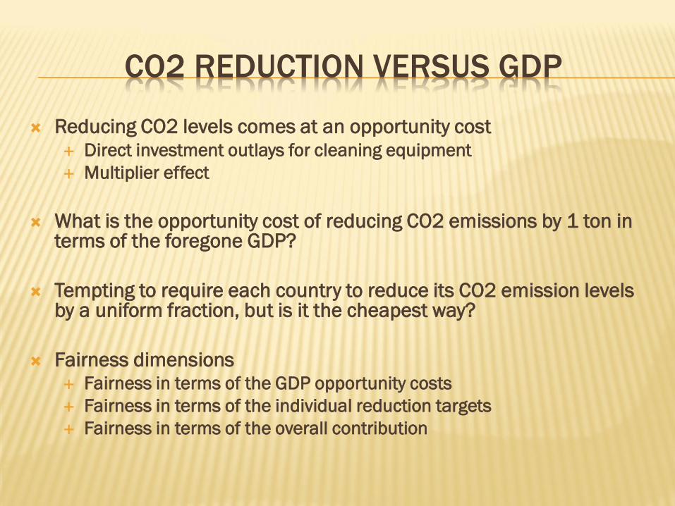
Reducing CO2 levels comes at an opportunity cost

Direct investment outlays for cleaning equipment

Multiplier effect

What is the opportunity cost of reducing CO2 emissions by 1 ton in terms of the foregone GDP?

Tempting to require each country to reduce its CO2 emission levels by a uniform fraction, but is it the cheapest way?

Fairness dimensions Fairness in terms of the GDP opportunity costs

Fairness in terms of the individual reduction targets

Fairness in terms of the overall contribution

MEASURING OPPORTUNITY COSTS OF CO2

REDUCTION IN TERMS OF GDP

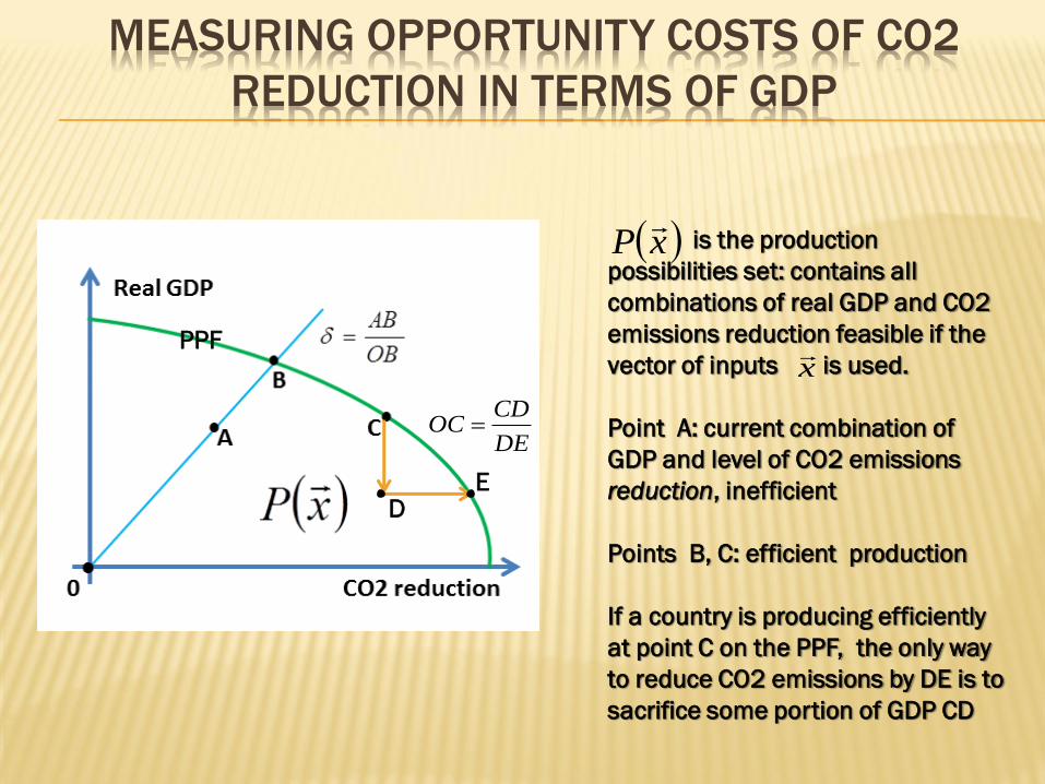
is the production

possibilities set: contains all

combinations of real GDP and CO2

emissions reduction feasible if the

vector of inputs is used.

Point A: current combination of

GDP and level of CO2 emissions

reduction, inefficient

Points B, C: efficient production

If a country is producing efficiently

at point C on the PPF, the only way

to reduce CO2 emissions by DE is to

sacrifice some portion of GDP CD

xP

x

D E

DE

CDOC

PPF

QUESTIONS TO ANSWER

What is the size of the costless reduction of

CO2 in the OECD countries?

What are the GDP opportunity costs of CO2

reduction for individual countries?

Which countries reduce CO2 cheaply?

Which countries reduce CO2 expensively?

What are the alternative scenarios of reducing

CO2 in the OECD countries?

ESTIMATION METHODOLOGY

Fare et al. (1993), Shephard’s duality lemma:

the opportunity costs of any two outputs can be

measured as a ratio of the two inputs’ shadow

prices

Equivalent to computing the slope of the PPF in

the two-dimensional space

Key assumption: one output’s shadow price is

equal to its market price

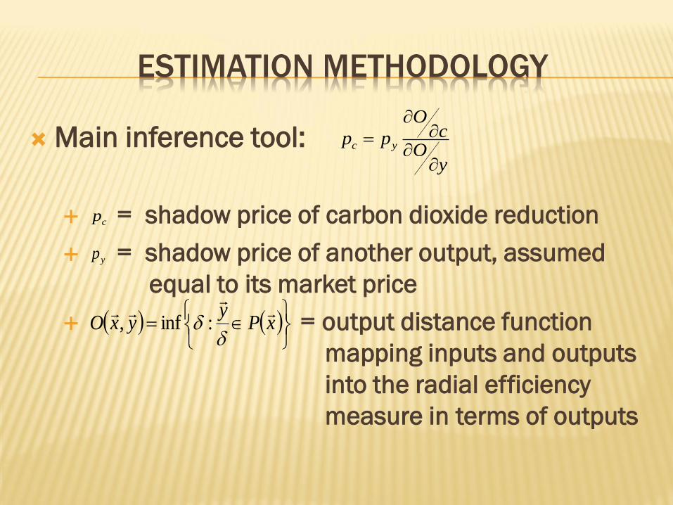
ESTIMATION METHODOLOGY

Main inference tool:

= shadow price of carbon dioxide reduction

= shadow price of another output, assumed

equal to its market price

= output distance function

mapping inputs and outputs

into the radial efficiency

measure in terms of outputs

yO

cO

pp yc

cp

yp

xPy

yxO

:inf,

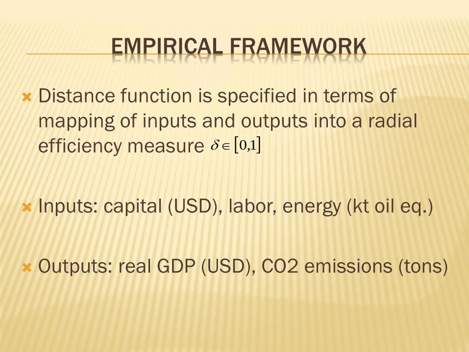
EMPIRICAL FRAMEWORK

Distance function is specified in terms of

mapping of inputs and outputs into a radial

efficiency measure

Inputs: capital (USD), labor, energy (kt oil eq.)

Outputs: real GDP (USD), CO2 emissions (tons)

1,0

EMPIRICAL FRAMEWORK

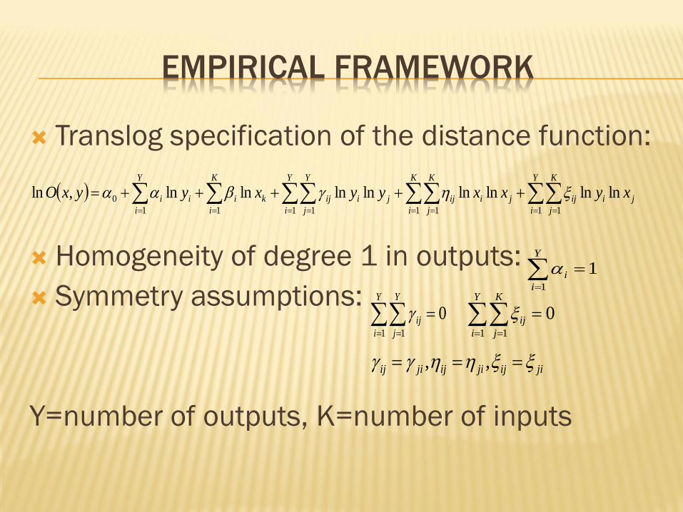
Translog specification of the distance function:

Homogeneity of degree 1 in outputs:

Symmetry assumptions:

Y=number of outputs, K=number of inputs

j

Y

i

K

j

iijj

K

i

K

j

iijj

Y

i

Y

j

iij

K

i

ki

Y

i

ii xyxxyyxyyxO lnlnlnlnlnlnlnln,ln1 11 11 111

0

11

Y

i

i

Y

i

Y

j

ij

1 1

0

Y

i

K

j

ij

1 1

0

jiijjiijjiij ,,

ESTIMATION OF DISTANCE FUNCTION

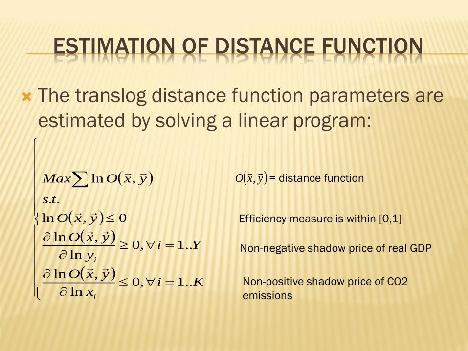
The translog distance function parameters are

estimated by solving a linear program:

Kix

yxO

Yiy

yxO

yxO

ts

yxOMax

i

i

..1,0ln

,ln

..1,0ln

,ln

0,ln

..

,ln

Efficiency measure is within [0,1]

Non-negative shadow price of real GDP

Non-positive shadow price of CO2

emissions

= distance function yxO

,

SHADOW COST OF REDUCING CO2

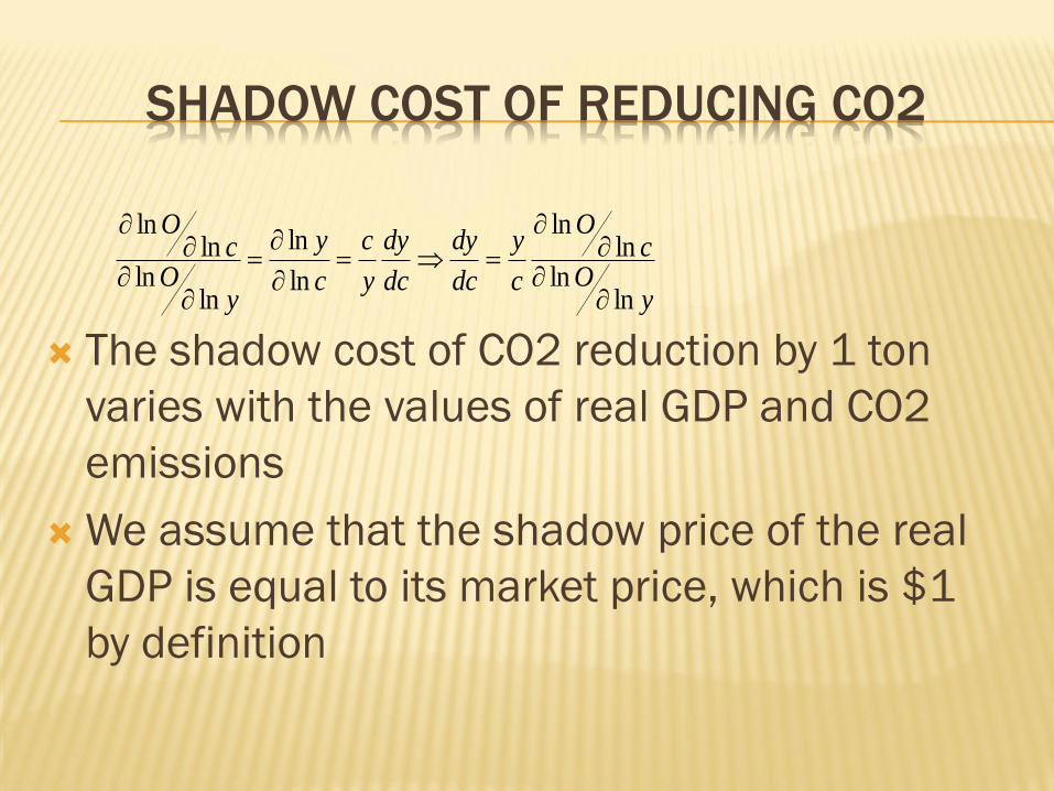
The shadow cost of CO2 reduction by 1 ton

varies with the values of real GDP and CO2

emissions

We assume that the shadow price of the real

GDP is equal to its market price, which is $1

by definition

yO

cO

c

y

dc

dy

dc

dy

y

c

c

y

yO

cO

lnln

lnln

ln

ln

lnln

lnln

DATA SOURCES

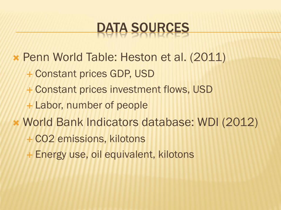
Penn World Table: Heston et al. (2011)

Constant prices GDP, USD

Constant prices investment flows, USD

Labor, number of people

World Bank Indicators database: WDI (2012)

CO2 emissions, kilotons

Energy use, oil equivalent, kilotons

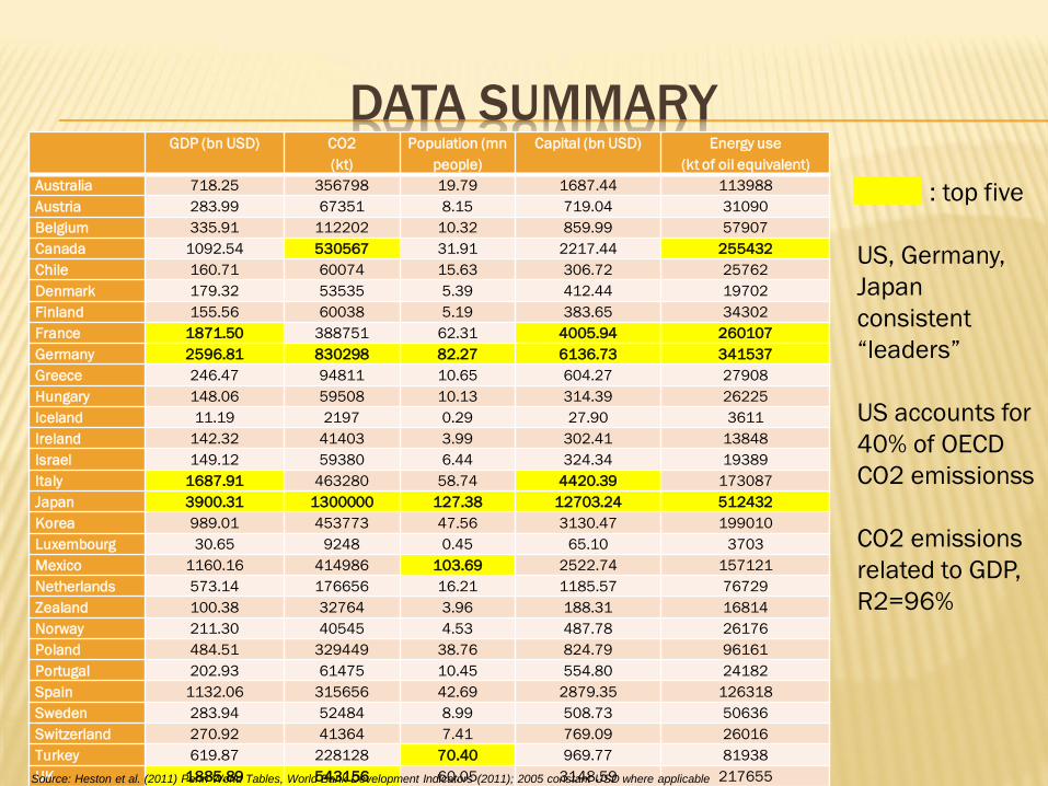
DATA SUMMARY GDP (bn USD) CO2

(kt)

Population (mn

people)

Capital (bn USD) Energy use

(kt of oil equivalent)

Australia 718.25 356798 19.79 1687.44 113988

Austria 283.99 67351 8.15 719.04 31090

Belgium 335.91 112202 10.32 859.99 57907

Canada 1092.54 530567 31.91 2217.44 255432

Chile 160.71 60074 15.63 306.72 25762

Denmark 179.32 53535 5.39 412.44 19702

Finland 155.56 60038 5.19 383.65 34302

France 1871.50 388751 62.31 4005.94 260107

Germany 2596.81 830298 82.27 6136.73 341537

Greece 246.47 94811 10.65 604.27 27908

Hungary 148.06 59508 10.13 314.39 26225

Iceland 11.19 2197 0.29 27.90 3611

Ireland 142.32 41403 3.99 302.41 13848

Israel 149.12 59380 6.44 324.34 19389

Italy 1687.91 463280 58.74 4420.39 173087

Japan 3900.31 1300000 127.38 12703.24 512432

Korea 989.01 453773 47.56 3130.47 199010

Luxembourg 30.65 9248 0.45 65.10 3703

Mexico 1160.16 414986 103.69 2522.74 157121

Netherlands 573.14 176656 16.21 1185.57 76729

Zealand 100.38 32764 3.96 188.31 16814

Norway 211.30 40545 4.53 487.78 26176

Poland 484.51 329449 38.76 824.79 96161

Portugal 202.93 61475 10.45 554.80 24182

Spain 1132.06 315656 42.69 2879.35 126318

Sweden 283.94 52484 8.99 508.73 50636

Switzerland 270.92 41364 7.41 769.09 26016

Turkey 619.87 228128 70.40 969.77 81938

UK 1885.89 543156 60.05 3148.59 217655

US 11534.05 5600000 289.87 23947.6 2200000

Source: Heston et al. (2011) Penn World Tables, World Bank Development Indicators (2011); 2005 constant USD where applicable

: top five

US, Germany,

Japan

consistent

“leaders”

US accounts for

40% of OECD

CO2 emissionss

CO2 emissions

related to GDP,

R2=96%

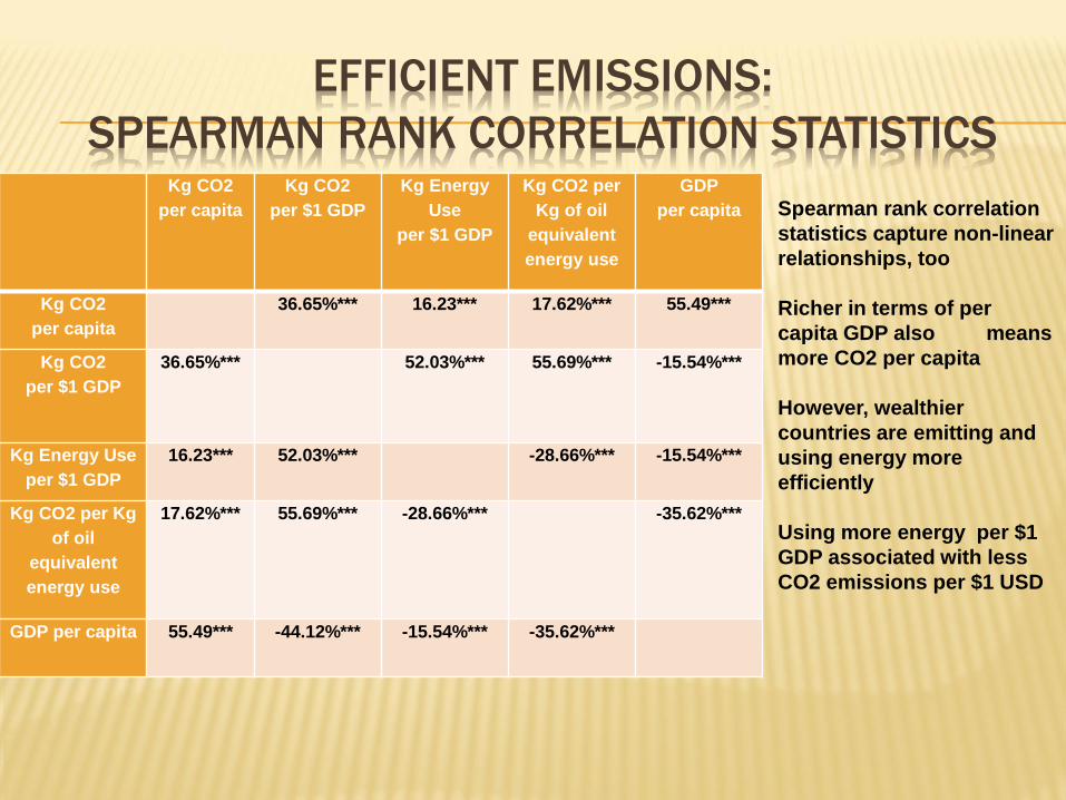
EFFICIENT EMISSIONS:

SPEARMAN RANK CORRELATION STATISTICS Kg CO2

per capita

Kg CO2

per $1 GDP

Kg Energy

Use

per $1 GDP

Kg CO2 per

Kg of oil

equivalent

energy use

GDP

per capita

Kg CO2

per capita

36.65%*** 16.23*** 17.62%*** 55.49***

Kg CO2

per $1 GDP

36.65%*** 52.03%*** 55.69%*** -15.54%***

Kg Energy Use

per $1 GDP

16.23*** 52.03%*** -28.66%*** -15.54%***

Kg CO2 per Kg

of oil

equivalent

energy use

17.62%*** 55.69%*** -28.66%*** -35.62%***

GDP per capita 55.49*** -44.12%*** -15.54%*** -35.62%***

Spearman rank correlation

statistics capture non-linear

relationships, too

Richer in terms of per

capita GDP also means

more CO2 per capita

However, wealthier

countries are emitting and

using energy more

efficiently

Using more energy per $1

GDP associated with less

CO2 emissions per $1 USD

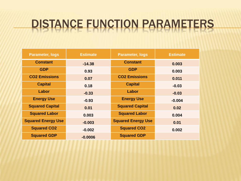
DISTANCE FUNCTION PARAMETERS

Parameter, logs Estimate Parameter, logs Estimate

Constant -14.38 Constant 0.003

GDP 0.93 GDP 0.003

CO2 Emissions 0.07 CO2 Emissions 0.011

Capital 0.18 Capital -0.03

Labor -0.33 Labor -0.03

Energy Use -0.93 Energy Use -0.004

Squared Capital 0.01 Squared Capital 0.02

Squared Labor 0.003 Squared Labor 0.004

Squared Energy Use -0.003 Squared Energy Use 0.01

Squared CO2 -0.002 Squared CO2 0.002

Squared GDP -0.0006 Squared GDP

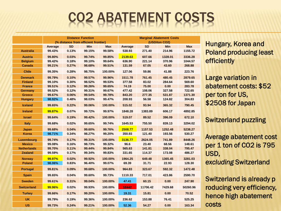
CO2 ABATEMENT COSTS

Distance Function

(% distance from efficient frontier)

Marginal Abatement Costs

(USD/ton CO2)

Average SD Min Max Average SD Min Max

Australia 99.43% 0.13% 99.15% 99.58% 538.93 271.40 214.96 1155.72

Austria 99.80% 0.03% 99.74% 99.85% 2139.63 607.66 1328.01 3336.28

Belgium 99.42% 0.18% 99.10% 99.64% 636.90 221.14 370.96 1044.57

Canada 99.21% 0.27% 98.68% 99.51% 131.59 67.05 43.60 268.88

Chile 99.35% 0.28% 98.75% 100.00% 127.06 59.86 41.88 223.76

Denmark 99.79% 0.10% 99.57% 99.96% 1511.78 761.45 480.45 2879.65

Finland 99.10% 0.30% 98.52% 99.53% 377.58 83.02 284.64 569.60

France 99.51% 0.12% 99.26% 99.65% 74.19 75.00 0.00 283.78

Germany 99.52% 0.12% 99.31% 99.67% 477.42 108.06 327.58 722.65

Greece 99.67% 0.06% 99.54% 99.78% 843.20 277.35 531.87 1371.30

Hungary 98.92% 0.48% 98.03% 99.47% 208.93 56.58 124.82 304.83

Iceland 99.65% 0.22% 99.06% 100.00% 515.02 93.94 365.32 790.45

Ireland 99.87% 0.07% 99.72% 99.97% 1848.28 1383.89 606.17 4892.85

Israel 99.64% 0.19% 99.42% 100.00% 519.07 89.52 396.09 672.10

Italy 99.68% 0.02% 99.65% 99.74% 1645.53 755.50 839.13 3294.02

Japan 99.68% 0.04% 99.60% 99.76% 2508.77 1157.53 1252.48 5238.27

Korea 98.71% 0.34% 98.27% 99.20% 350.93 121.40 193.56 530.27

Luxembourg 99.74% 0.17% 99.31% 100.00% 3136.77 2624.05 741.89 8448.26

Mexico 99.08% 0.16% 98.73% 99.32% 96.6 23.40 68.56 148.61

Netherlands 99.70% 0.11% 99.44% 99.84% 565.63 141.81 338.04 795.47

Zealand 99.59% 0.17% 99.34% 99.83% 331.65 114.37 173.08 486.27

Norway 99.97% 0.02% 99.92% 100.00% 1964.25 649.48 1365.45 3281.03

Poland 98.06% 0.83% 96.40% 99.07% 69.39 31.71 22.93 128.30

Portugal 99.81% 0.09% 99.68% 100.00% 964.83 323.67 592.32 1472.48

Spain 99.65% 0.04% 99.60% 99.73% 1110.33 717.01 423.86 2590.70

Sweden 99.61% 0.31% 99.04% 100.00% 47.41 60.15 0.00 247.90

Switzerland 99.96% 0.02% 99.93% 100.00% 18442 11706.42 7429.68 50260.96

Turkey 99.66% 0.17% 99.20% 100.00% 19.31 15.81 0.00 70.52

UK 99.79% 0.19% 99.36% 100.00% 236.62 153.88 76.41 525.25

US 99.73% 0.24% 99.21% 100.00% 52.36 54.27 0.00 163.34

Hungary, Korea and

Poland producing least

efficiently

Large variation in

abatement costs: $52

per ton for US,

$2508 for Japan

Switzerland puzzling

Average abatement cost

per 1 ton of CO2 is 795

USD,

excluding Switzerland

Switzerland is already p

roducing very efficiency,

hence high abatement

costs

CO2 ABATEMENT COSTS AND

POLLUTION TRADING PERMITS

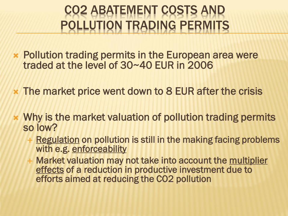
Pollution trading permits in the European area were traded at the level of 30~40 EUR in 2006

The market price went down to 8 EUR after the crisis

Why is the market valuation of pollution trading permits so low? Regulation on pollution is still in the making facing problems

with e.g. enforceability

Market valuation may not take into account the multiplier effects of a reduction in productive investment due to efforts aimed at reducing the CO2 pollution

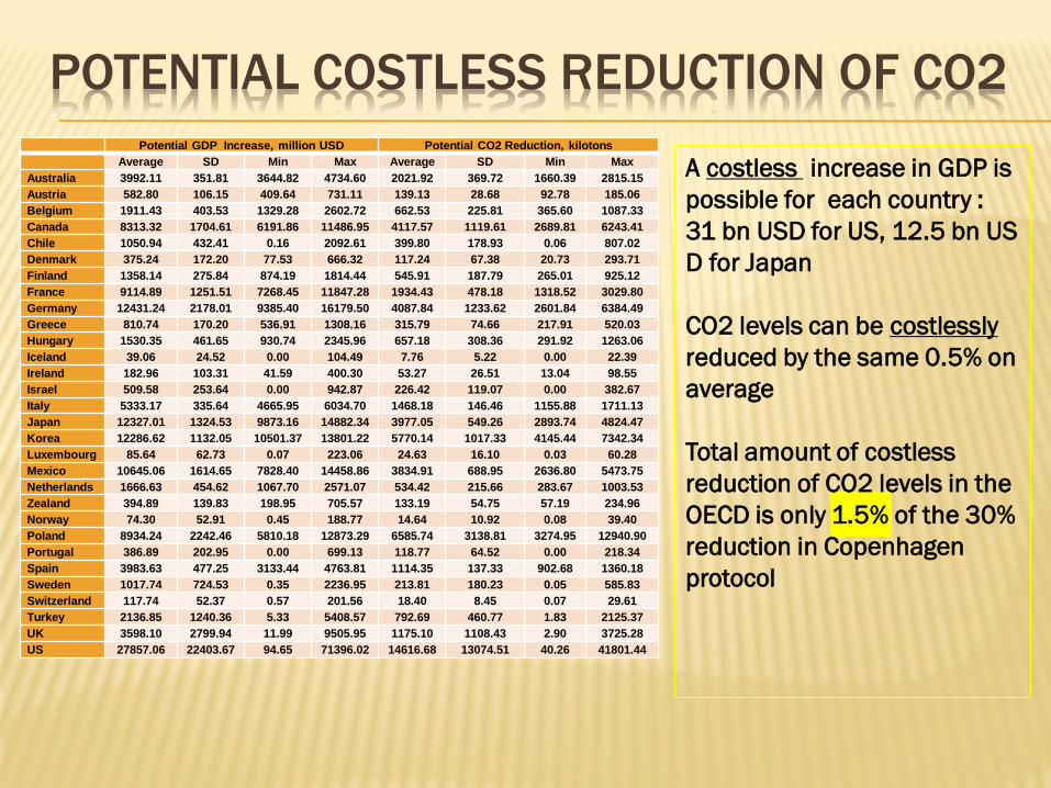
POTENTIAL COSTLESS REDUCTION OF CO2

Potential GDP Increase, million USD Potential CO2 Reduction, kilotons

Average SD Min Max Average SD Min Max

Australia 3992.11 351.81 3644.82 4734.60 2021.92 369.72 1660.39 2815.15

Austria 582.80 106.15 409.64 731.11 139.13 28.68 92.78 185.06

Belgium 1911.43 403.53 1329.28 2602.72 662.53 225.81 365.60 1087.33

Canada 8313.32 1704.61 6191.86 11486.95 4117.57 1119.61 2689.81 6243.41

Chile 1050.94 432.41 0.16 2092.61 399.80 178.93 0.06 807.02

Denmark 375.24 172.20 77.53 666.32 117.24 67.38 20.73 293.71

Finland 1358.14 275.84 874.19 1814.44 545.91 187.79 265.01 925.12

France 9114.89 1251.51 7268.45 11847.28 1934.43 478.18 1318.52 3029.80

Germany 12431.24 2178.01 9385.40 16179.50 4087.84 1233.62 2601.84 6384.49

Greece 810.74 170.20 536.91 1308.16 315.79 74.66 217.91 520.03

Hungary 1530.35 461.65 930.74 2345.96 657.18 308.36 291.92 1263.06

Iceland 39.06 24.52 0.00 104.49 7.76 5.22 0.00 22.39

Ireland 182.96 103.31 41.59 400.30 53.27 26.51 13.04 98.55

Israel 509.58 253.64 0.00 942.87 226.42 119.07 0.00 382.67

Italy 5333.17 335.64 4665.95 6034.70 1468.18 146.46 1155.88 1711.13

Japan 12327.01 1324.53 9873.16 14882.34 3977.05 549.26 2893.74 4824.47

Korea 12286.62 1132.05 10501.37 13801.22 5770.14 1017.33 4145.44 7342.34

Luxembourg 85.64 62.73 0.07 223.06 24.63 16.10 0.03 60.28

Mexico 10645.06 1614.65 7828.40 14458.86 3834.91 688.95 2636.80 5473.75

Netherlands 1666.63 454.62 1067.70 2571.07 534.42 215.66 283.67 1003.53

Zealand 394.89 139.83 198.95 705.57 133.19 54.75 57.19 234.96

Norway 74.30 52.91 0.45 188.77 14.64 10.92 0.08 39.40

Poland 8934.24 2242.46 5810.18 12873.29 6585.74 3138.81 3274.95 12940.90

Portugal 386.89 202.95 0.00 699.13 118.77 64.52 0.00 218.34

Spain 3983.63 477.25 3133.44 4763.81 1114.35 137.33 902.68 1360.18

Sweden 1017.74 724.53 0.35 2236.95 213.81 180.23 0.05 585.83

Switzerland 117.74 52.37 0.57 201.56 18.40 8.45 0.07 29.61

Turkey 2136.85 1240.36 5.33 5408.57 792.69 460.77 1.83 2125.37

UK 3598.10 2799.94 11.99 9505.95 1175.10 1108.43 2.90 3725.28

US 27857.06 22403.67 94.65 71396.02 14616.68 13074.51 40.26 41801.44

A costless increase in GDP is

possible for each country :

31 bn USD for US, 12.5 bn US

D for Japan

CO2 levels can be costlessly

reduced by the same 0.5% on

average

Total amount of costless

reduction of CO2 levels in the

OECD is only 1.5% of the 30%

reduction in Copenhagen

protocol

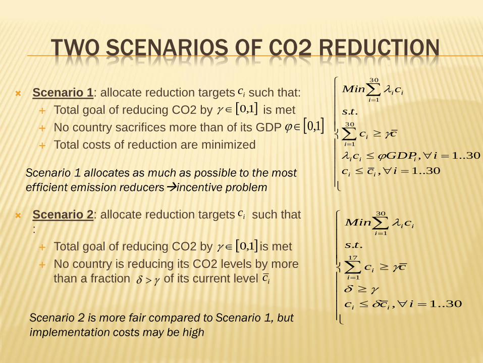
TWO SCENARIOS OF CO2 REDUCTION

Scenario 1: allocate reduction targets such that:

Total goal of reducing CO2 by is met

No country sacrifices more than of its GDP

Total costs of reduction are minimized

Scenario 2: allocate reduction targets such that

:

Total goal of reducing CO2 by is met

No country is reducing its CO2 levels by more

than a fraction of its current level

1,0

1,0

30..1,

30..1,

..

30

1

30

1

icc

iGDPc

cc

ts

cMin

ii

iii

i

i

i

ii

ic

ic

1,0

ic

30..1,

..

17

1

30

1

icc

cc

ts

cMin

ii

i

i

i

ii

Scenario 1 allocates as much as possible to the most

efficient emission reducersincentive problem

Scenario 2 is more fair compared to Scenario 1, but

implementation costs may be high

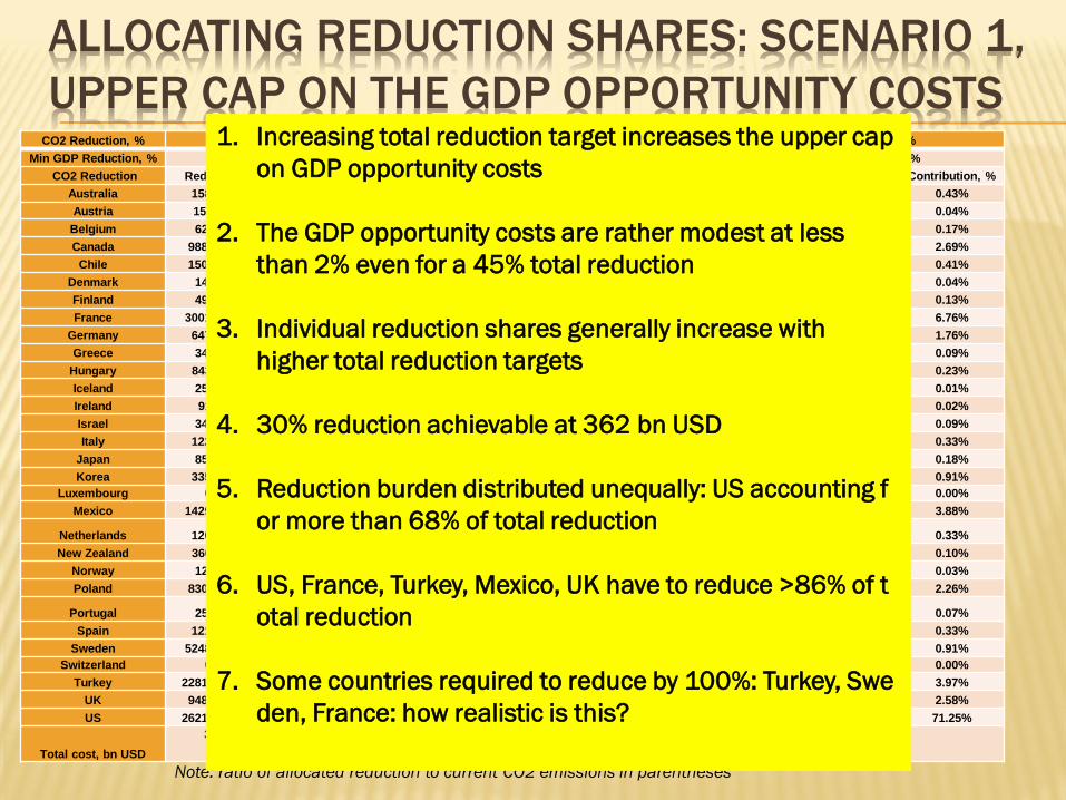
ALLOCATING REDUCTION SHARES: SCENARIO 1,

UPPER CAP ON THE GDP OPPORTUNITY COSTS CO2 Reduction, % 30% 35% 40% 45%

Min GDP Reduction, % 1.19% 1.40% 1.62% 1.86%

CO2 Reduction Reduction, kt Contribution, % Reduction, kt Contribution, % Reduction, kt Contribution, % Reduction, kt Contribution, %

Australia 15860 (4%) 0.41% 18658 (5%) 0.42% 21590 (6%) 0.42% 24789 (7%) 0.43%

Austria 1579 (2%) 0.04% 1858 (3%) 0.04% 2150 (3%) 0.04% 2469 (4%) 0.04%

Belgium 6276 (6%) 0.16% 7384 (7%) 0.17% 8544 (8%) 0.17% 9810 (9%) 0.17%

Canada 98801 (19%) 2.58% 116236 (22%) 2.60% 134502 (25%) 2.63% 154428 (29%) 2.69%

Chile 15052 (25%) 0.39% 17708 (29%) 0.40% 20490 (34%) 0.40% 23526 (39%) 0.41%

Denmark 1412 (3%) 0.04% 1661 (3%) 0.04% 1922 (4%) 0.04% 2206 (4%) 0.04%

Finland 4903 (8%) 0.13% 5768 (10%) 0.13% 6674 (11%) 0.13% 7663 (13%) 0.13%

France 300187 (77%) 7.83% 353161 (91%) 7.90% 388751 (100%) 7.60% 388751 (100%) 6.76%

Germany 64727 (8%) 1.69% 76150 (9%) 1.70% 88116 (11%) 1.72% 101170 (12%) 1.76%

Greece 3478 (4%) 0.09% 4092 (4%) 0.09% 4735 (5%) 0.09% 5437 (6%) 0.09%

Hungary 8433 (14%) 0.22% 9921 (17%) 0.22% 11480 (19%) 0.22% 13181 (22%) 0.23%

Iceland 259 (12%) 0.01% 304 (14%) 0.01% 352 (16%) 0.01% 404 (18%) 0.01%

Ireland 916 (2%) 0.02% 1078 (3%) 0.02% 1247 (3%) 0.02% 1432 (3%) 0.02%

Israel 3419 (6%) 0.09% 4022 (7%) 0.09% 4654 (8%) 0.09% 5343 (9%) 0.09%

Italy 12206 (3%) 0.32% 14361 (3%) 0.32% 16617 (4%) 0.33% 19079 (4%) 0.33%

Japan 8502 (1%) 0.22% 21765 (2%) 0.49% 25186 (2%) 0.49% 10093 (1%) 0.18%

Korea 33537 (7%) 0.87% 39456 (9%) 0.88% 45656 (10%) 0.89% 52420 (12%) 0.91%

Luxembourg 0 (0%) 0.00% 137 (1%) 0.00% 158 (2%) 0.00% 0 (0%) 0.00%

Mexico 142918 (34%) 3.73% 168139 (41%) 3.76% 194561 (47%) 3.81% 223385 (54%) 3.88%

Netherlands 12058 (7%) 0.31% 14186 (8%) 0.32% 16415 (9%) 0.32% 18847 (11%) 0.33%

New Zealand 3602 (11%) 0.09% 4237 (13%) 0.09% 4903 (15%) 0.10% 5630 (17%) 0.10%

Norway 1280 (3%) 0.03% 1506 (4%) 0.03% 1743 (4%) 0.03% 2001 (5%) 0.03%

Poland 83091 (25%) 2.17% 97754 (30%) 2.19% 113115 (34%) 2.21% 129873 (39%) 2.26%

Portugal 2503 (4%) 0.07% 2945 (5%) 0.07% 3407 (6%) 0.07% 3912 (6%) 0.07%

Spain 12133 (4%) 0.32% 14274 (5%) 0.32% 16517 (5%) 0.32% 18964 (6%) 0.33%

Sweden 52484 (100%) 1.37% 52484 (100%) 1.17% 52484 (100%) 1.03% 52484 (100%) 0.91%

Switzerland 0 (0%) 0.00% 33 (0%) 0.00% 141 (0%) 0.00% 0 (0%) 0.00%

Turkey 228128 (100%) 5.95% 228128 (100%) 5.10% 228128 (100%) 4.46% 228128 (100%) 3.97%

UK 94844 (17%) 2.47% 111582 (21%) 2.49% 129116 (24%) 2.53% 148244 (27%) 2.58%

US 2621375 (47%) 68.37% 3083971 (55%) 68.95% 3568595 (64%) 69.81% 4097275 (73%) 71.25%

Total cost, bn USD

362.06

455.27

526.16 548.03

Note: ratio of allocated reduction to current CO2 emissions in parentheses

1. Increasing total reduction target increases the upper cap

on GDP opportunity costs

2. The GDP opportunity costs are rather modest at less

than 2% even for a 45% total reduction

3. Individual reduction shares generally increase with

higher total reduction targets

4. 30% reduction achievable at 362 bn USD

5. Reduction burden distributed unequally: US accounting f

or more than 68% of total reduction

6. US, France, Turkey, Mexico, UK have to reduce >86% of t

otal reduction

7. Some countries required to reduce by 100%: Turkey, Swe

den, France: how realistic is this?

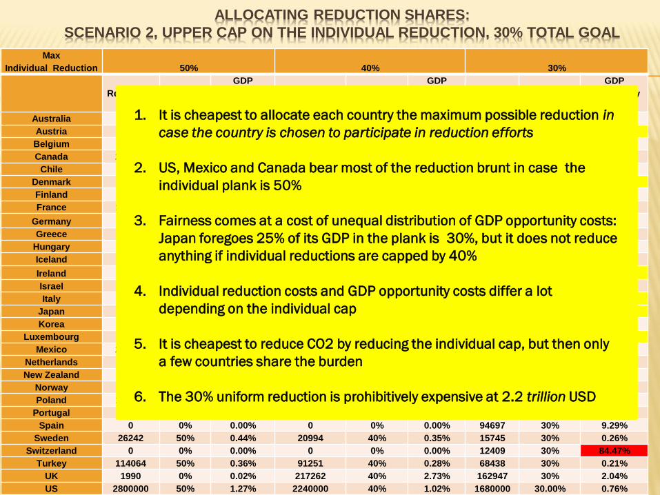
ALLOCATING REDUCTION SHARES:

SCENARIO 2, UPPER CAP ON THE INDIVIDUAL REDUCTION, 30% TOTAL GOAL

Max

Individual Reduction 50% 40% 30%

Reduction,

kt

Relative

to current

GDP

opportunity

costs

Reduction,

kt

Relative to

current

GDP

opportunity

costs

Reduction,

kt

Relative to

current

GDP

opportunity

costs

Australia 0 0% 0.00% 0 0% 0.00% 107039 30% 8.03%

Austria 0 0% 0.00% 0 0% 0.00% 20205 30% 15.22%

Belgium 0 0% 0.00% 0 0% 0.00% 33661 30% 6.38%

Canada 265284 50% 3.20% 212227 40% 2.56% 159170 30% 1.92%

Chile 30037 50% 2.37% 24030 40% 1.90% 18022 30% 1.42%

Denmark 0 0% 0.00% 0 0% 0.00% 16061 30% 13.54%

Finland 0 0% 0.00% 24015 40% 5.83% 18011 30% 4.37%

France 194376 50% 0.77% 155500 40% 0.62% 116625 30% 0.46%

Germany 0 0% 0.00% 332119 40% 6.11% 249089 30% 4.58%

Greece 0 0% 0.00% 0 0% 0.00% 28443 30% 9.73%

Hungary 29754 50% 4.20% 23803 40% 3.36% 17852 30% 2.52%

Iceland 0 0% 0.00% 373 17% 1.72% 659 30% 3.03%

Ireland 0 0% 0.00% 0 0% 0.00% 12421 30% 16.13%

Israel 0 0% 0.00% 0 0% 0.00% 17814 30% 6.20%

Italy 0 0% 0.00% 0 0% 0.00% 138984 30% 13.55%

Japan 0 0% 0.00% 0 0% 0.00% 390000 30% 25.09%

Korea 0 0% 0.00% 181509 40% 6.44% 136132 30% 4.83%

Luxembourg 0 0% 0.00% 0 0% 0.00% 2774 30% 28.39%

Mexico 207493 50% 1.73% 165994 40% 1.38% 124496 30% 1.04%

Netherlands 0 0% 0.00% 0 0% 0.00% 52997 30% 5.23%

New Zealand 0 0% 0.00% 13106 40% 4.33% 9829 30% 3.25%

Norway 0 0% 0.00% 0 0% 0.00% 12164 30% 11.31%

Poland 164725 50% 2.36% 131780 40% 1.89% 98835 30% 1.42%

Portugal 0 0% 0.00% 0 0% 0.00% 18443 30% 8.77%

Spain 0 0% 0.00% 0 0% 0.00% 94697 30% 9.29%

Sweden 26242 50% 0.44% 20994 40% 0.35% 15745 30% 0.26%

Switzerland 0 0% 0.00% 0 0% 0.00% 12409 30% 84.47%

Turkey 114064 50% 0.36% 91251 40% 0.28% 68438 30% 0.21%

UK 1990 0% 0.02% 217262 40% 2.73% 162947 30% 2.04%

US 2800000 50% 1.27% 2240000 40% 1.02% 1680000 30.00% 0.76%

Total cost, bn USD 241.36 479.99 2184.49

1. It is cheapest to allocate each country the maximum possible reduction in

case the country is chosen to participate in reduction efforts

2. US, Mexico and Canada bear most of the reduction brunt in case the

individual plank is 50%

3. Fairness comes at a cost of unequal distribution of GDP opportunity costs:

Japan foregoes 25% of its GDP in the plank is 30%, but it does not reduce

anything if individual reductions are capped by 40%

4. Individual reduction costs and GDP opportunity costs differ a lot

depending on the individual cap

5. It is cheapest to reduce CO2 by reducing the individual cap, but then only

a few countries share the burden

6. The 30% uniform reduction is prohibitively expensive at 2.2 trillion USD

CONCLUSIONS

Basic tradeoff between uniformity of individual reductions and GDP opportunity costs

Uniform reductions at 30% “Copenhagen” levels are prohibitively expensive relative to other scenarios

Need additional criteria to choose individual reduction planks or GDP opportunity costs

Additional research needed to explore the dynamic optimality of CO2 reductions