2010 – 2030

Water Resource Plan

Appendix B

December 2009

Appendix B:

Climate Change Studies

Potential Climate Change and Impacts on Water Resources

prepared by

Mark Stone, Ph.D.

Division of Hydrologic Sciences

Desert Research Institute

Hilary Lopez, Ph.D.

Truckee Meadows Water Authority

prepared for

Truckee Meadows Water Authority

1355 Capital Boulevard

Reno, NV 89520

July 2006

1

Potential Climate Change and Impacts on Water Resources

Abstract

As a natural process of the climate system, the Earth's climate has been forever changing.

Climate change in the last 100 years, however, is thought to have been influenced by human activities, in

particular greenhouse gas (GHG) emissions. Early signs of this change, such as increased mean annual

temperatures and thinner sea ice, have been observed in many regions of the world. According to global

climate models, continued increases in greenhouse gas emissions could cause further changes in

temperature, with the global mean temperature potentially rising by approximately 2.7 to 10.4º F by 2100.

This potential change in climate could cause changes in atmospheric and oceanic circulation patterns,

and in the hydrologic cycle, leading to altered patterns of precipitation and runoff. Warmer temperatures

will potentially increase moisture availability and precipitation. However in mountainous regions, such as

the Sierra Nevada, a larger fraction of the total precipitation could be in the form of rain, resulting in

shorter snow accumulation periods, reduced annual snowpacks, earlier spring melting, and reduced

summer flows. To plan effectively, it is important to understand how and why climate may change in the

future and how that may affect water resources. The goal of this document is to summarize the current

state-of-knowledge of climate change as it relates to water resources in the western United States.

Climate Change and Global Warming

As a natural process of the climate system, the Earth’s climate has been forever changing. Most

recently, within the past 100 years, scientists have witnessed a general warming trend in temperatures

termed “global warming.” Additionally, this “warming” seems to have accelerated during the past two

decades. While natural processes contribute to global warming, it is also widely believed that human

activities are attributing to the rapid temperature rise. A majority of scientists contend that human

activities have “altered the chemical composition of the atmosphere through the buildup of greenhouse

gases – primarily carbon dioxide, methane, and nitrous oxide” – and that this buildup has resulted in

rising global temperatures (US EPA). However, it is important to point out that within the scientific

community controversy continues regarding the extent and effects of human impacts on global climate

change.

Atmospheric Greenhouse Gas and Aerosol Concentrations

The major greenhouse gasses, carbon dioxide, methane, nitrous oxide and water vapor, occur

naturally in the atmosphere. These greenhouse gases trap and retain energy in the Earth’s atmosphere

and help keep temperatures hospitable. When there is an elevated buildup of these gases in the

atmosphere, however, problems may arise. Human activities are releasing large quantities of these

substances into the atmosphere. For example, according to the US Environmental Protection Agency (US

EPA) since the beginning of the industrial revolution atmospheric concentrations of carbon dioxide have

2

increased nearly 30%, methane concentrations have more than doubled, and nitrous oxide

concentrations have risen by about 15%.

While concentrations of carbon dioxide (CO2) have increased, the exact source of the recent rise

in atmospheric CO2 has not been determined with certainty. It is likely caused by an interacting

combination of natural and anthropogenic forces. This appears reasonable because the magnitudes of

human release and atmospheric rise are comparable, and the atmospheric rise has occurred

contemporaneously with the increase in production of CO2 from human activities following the Industrial

Revolution (Soon et al. 1999). However, the factors that influence CO2 concentrations are not fully

understood. The current increase in CO2 follows a 300 year warming trend following a Little Ice Age

(Keigwin 1996). Some have hypothesized that the recent changes in atmospheric CO2 can be explained

by the oceans emitting gases naturally as temperatures rise following the Little Ice Age (Segalstad 1998).

However, the expected associated drop in ocean CO2 concentrations has not been observed (Sabine et

al. 2004).

Human activities have also increased concentrations of atmospheric aerosols (microscopic,

airborne particles) since pre-industrial times. Aerosols are emitted by industrial processes (fossil-fuel

combustion and biomass burning) and their increased concentration offsets simultaneous warming by

reducing solar radiation to the ground. Unlike greenhouse gases, which are generally long-lived, aerosols

fall out of the atmosphere fairly rapidly, either dry (through sedimentation) or within rain (as condensation

nuclei), and therefore are not uniformly mixed across the globe.

Atmospheric composition will continue to change throughout the 21st century. The

Intergovernmental Panel on Climate Change (IPCC) Special Report on Emission Scenarios (SRES)(IPCC

2000) summarizes the results of global climate models that were used to forecast atmospheric

concentrations of greenhouse gases based upon a range of emission scenarios. According to the IPCC

report, emissions of CO2 due to fossil fuel burning will strongly influence trends in atmospheric CO2

concentration during the 21st century. By 2100, atmospheric CO2 concentrations are projected between

540 to 970 ppm (90 to 250% above the concentration of 280 ppm in the year 1750). These projections

include land and ocean climate feedbacks.

Global Temperature Records

Records show a measurable warming trend in the Earth’s surface temperature over the past 100

years, with a rapid acceleration in warming over the past two decades (Figure 1). Over the past century,

the global average surface temperature has increased by approximately 1º F (0.5º C). Further, 9 of the 10

warmest years on record have occurred since 1995. According to recent data released by the National

Climatic Data Center (www.ncdc.noaa.gov), 2005 was likely the warmest or second warmest year in the

global instrumental temperature record.

3

The Earth’s surface temperature varies naturally over a wide range, but available temperature

records are spatially and temporally limited. Records going back longer than 350 years are reconstructed

from proxies. Reconstructed data produced from tree ring width, ice cores, and sedimentary deposits

contain important limitations due to their required interpretation. For example, tree width and density

have become less sensitive to changes in temperature over the last few decades (Briffa et al. 1998). The

limited spatial extent of surface records results in only 18.4% of the Earth’s surface being accurately

described by direct measurement (Michaels et al. 2000). Further, the influence of land use change on

temperature records is known to affect measurements through the urban heat island phenomenon. This

systematic error has been extensively studied and debated. Peterson et al. (2003) found a bias in urban

stations after 1990 at several stations. The researchers described the need to reassess designations of

surface temperature stations as urban, suburban, or rural on a periodical basis.

Complex three-dimensional coupled ocean-atmosphere general circulation models (GCMs) can

be used to predict future climate conditions under various greenhouse gas emission scenarios. Using an

ensemble of GCMs and emission scenarios, the IPCC (IPCC WGI 2001) produced the range of predicted

CO2 and temperature changes shown in Figure 2. The globally averaged surface temperature is projected

to increase by 2.7° to 10.4°F (1.4 to 5.8°C) over the period of 1990 to 2100. The projected rate of

warming is much larger than the observed changes during the 20th century and very likely would be

without precedent during at least the last 10,000 years. However, these models contain sources of

uncertainty and there is a variety of debate with regards to these model predictions. An overview of the

sources of uncertainty and debate is provided below.

Figure1. Global

mean land and

sea-surface

temperature

anomalies for the

duration of the

instrumental record

(Australian Bureau

of Meteorology).

4

Sources of Uncertainty

As discussed above, the IPCC estimates that global average temperature will rise by between

2.7° to 10.4°F by the year 2100. Although climate models estimate that temperatures may warm,

opponents of global warming theories point out that climate science cannot make definitive predictions yet

because many of the physical processes modeled are only rudimentarily understood and are variously

parameterized. Because the climate is a coupled, non-linear dynamic system, the climate models have

many uncertainties. Without experimental validation of the models, the calculation of the climate

response to increased anthropogenic atmospheric CO2 will remain in doubt. For example, opponents of

global warming theories that attribute temperature rise to human activities argue that the correlation

between rising temperatures and CO2 concentrations following the Industrial Revolution does not prove

causation. The US EPA further reiterates the warning provided by all climate modelers to people

considering the impacts of future climate change: the projections of climate change in specific areas are

not forecasts but are reasonable examples of how the climate might change (US EPA).

The two primary sources of uncertainty are 1) forecasts of future greenhouse gas emissions; and

2) the nature of many feedback processes in the climate system. Future GHG emissions depend on the

rate of growth of the world’s economy and population, generation of energy technology, land use

changes, and policies aimed at reducing emissions. Feedback processes may strongly influence global

warming. For example, increased atmospheric water vapor may amplify warming, while changes in the

extent of cloud cover and the characteristics of clouds may either enhance or diminish warming. Soon et

al. (1999) discussed the following six important areas of uncertainty and error in climate modeling.

1) Water vapor feedback - The feedback process starts with increasing temperature that increases

atmospheric water vapor concentration. Water vapor is itself a strong greenhouse agent, which in

turn could amplify the warming caused by elevated CO2. The model parameterization used to

Figure 2. Atmospheric CO2 concentrations scenarios and simulated changes in global temperature

(Australian Bureau of Meteorology).

5

describe this feedback mechanism is complex and has received criticism (e.g. Renno et al. 1994).

Without adequate observations, it is difficult to determine the correct parameterization.

2) Cloud forcing – Climate models produce different projected temperature changes because they

incorporate different estimates of the parameters that describe the behavior of cloud formation.

Clouds are known to have an important influence on surface temperatures. However, current

GCMs over-predict the coverage of high clouds by a factor as large as 2 to 5. The spatial

distribution of clouds is also incorrect. Therefore, the parameterization of radiative, latent and

convective effects of cloud forcing needs further improvements.

3) Ocean-atmospheric interaction – The dynamic nature of air-sea coupling is complex and requires

intense in situ and satellite observations of heat, momentum, and freshwater fluxes. This is an

active area of GCM research.

4) Sea-ice-snow feedback – Currently, GCM results under-predict the variance of sea-ice thickness

in the Arctic on decadal to century time scales. This result emphasizes the importance of

including realistic surface fluxes and modeling of convective overturning and vertical advection in

both the Arctic and adjacent oceans.

5) Biosphere-atmosphere-ocean feedback – Biospheric feedback influences the global carbon

budget because enhanced plant growth will sequester CO2. Understanding this feedback holds

the promise of an internally consistent description of the relationship of CO2 to climate change.

6) Flux errors – Many models have substantial flux errors for which calibration adjustments are

introduced into the calculations. One important consequence is the dampening of low-frequency

variability in the simulation of climate state due to over stabilization.

The impacts of feedback mechanisms on predicted temperature are shown in Figure 3. Accounting

for the range of uncertainty in these feedback processes results in a range of possible changes in global

average temperatures for any given change in GHG concentrations. The range of temperature changes

projected by the IPCC reflects the combined effects of all of these sources of uncertainty. Further, even

greater uncertainty exists in regional predictions of climate change. Regional projections of impacts are

most needed by decision-makers, and yet are not easily extracted from global climate model simulations.

Results can sometimes even be contradictory at the regional scale, with either wetter or drier conditions

predicted depending on the model used for the simulation.

6

Potential Impacts of Climate Change on Water Resources

Although the science of climate change and predictions of future temperature and precipitation

remain largely uncertain (particularly at the regional level), it is still appropriate to consider the potential

impacts of such change on water resources. This information will enhance our ability to respond to

change as the science advances and uncertainty is reduced. In this section, observed changes in

hydrologic processes corresponding with recent warming trends in the western U.S. and potential impacts

of future climate change on hydrologic processes are discussed.

Potential changes to the climate will likely alter the hydrologic cycle in ways that impact water

resources. Regional climate-change projections are uncertain. However, the magnitude of projected

warming combined with a strong regional reliance on mountain snowpack creates some consistency in

the implication of climate change for the western U.S. The amount, intensity, and temporal distribution of

precipitation could potentially change. Recent research suggests an intensification of the global

Figure 3. Schematic showing the

influence of climate feedbacks

on radiative forcing driving a

climate model. The arrows are

indicative of the magnitude and

sign of individual feedbacks

(Australian Bureau of

Meteorology).

7

hydrological cycle, leading to more intense but possibly less frequent periods of precipitation (longer

periods of drought alternating with spells of heavy rainfall) (Trenberth 2003). In the west, warmer

temperatures could affect the proportion of winter precipitation falling as rain or snow, accumulation of

snowpack, and snowmelt timing. Evapotranspiration could change with changes in soil moisture

availability, and plant responses to elevated CO2 concentrations. In addition, changes in the quantity of

water percolating to groundwater storage could result in changes in aquifer levels, in base flows entering

surface streams, and in seepage losses from surface water bodies to the groundwater system.

The overall scientific consensus is that globally the

Earth will be warmer with higher globally averaged precipitation.

However, current scientific understanding does not provide

confident projections of the magnitude or precise nature of

changed precipitation patterns. Unlike the projections of

precipitation change, climate models are fairly consistent in

predictions of regional surface temperature. Because

temperature is central in determining the accumulation and

melting of snow and ice, these scenarios are especially relevant

to regions where snowpack dominates the hydrology. Even with

wetter winters, a warmer climate will result in a greater portion

of winter precipitation falling as rain rather than snow, an

elevated winter snowline, and a decrease in the snow-covered

areas and total winter snowpack (Figure 4). Some of the most

sensitive areas are where winter temperatures are now only

slightly below freezing. Temperature also determines the timing

of melt-off, and a warmer climate will likely result in an earlier melt season. Many regions are likely to see

an increase in winter or early spring stream flows and reduced summer flows.

The results of warmer temperatures have been observed across the western U.S. Winter and

spring temperatures have increased in western North America during the twentieth century (Folland et al.

2001), and there is a large body of evidence suggesting this widespread warming has produced changes

in hydrology and plants. In the western U.S and southwestern Canada, spring snowpacks have been

smaller and have been melting earlier in most mountain areas. Snow extent and depth have generally

decreased in the west (Mote 2003). These declines have often occurred despite increases in total winter

precipitation in those locations. The timing of spring snowmelt-driven streamflow has shifted earlier in the

year (Cayan et al. 2001; Stewart et al. 2005), as is expected in a warming climate (Figure 5). There has

also been a century-long downward trend in late spring and early summer flow as a proportion of total

annual flow (Dettinger and Cayan 1995). Earlier spring melting and reduced spring snowpacks have been

especially evident in the Cascade and northern Sierra Nevada Mountains, where winter temperatures are

relatively mild. Some higher elevation mountain locations in the Southern Sierra Nevada and Rocky

Figure 4. Linear trends in 1 Apr SWE

for 1950–97 from a hydrologic

simulation (Mote et al. 2003).

8

Mountain ranges have shown an increasing trend in

April 1 snowpacks, but even there the peak in spring

runoff is generally occurring earlier (Stewart et al.

2004).

Dettinger et al. (2004) completed a simulation

of hydrologic response to climate variation and

change in three Sierra Nevada watersheds (including

the Carson River watershed). The research used

climate predictions from a GCM coupled with a

hydrologic model to investigate future changes in

streamflow. Although the climate model projections

were near the lower edge of the available climate

change simulations, in terms of warming and

changes in precipitation, the results still showed

significant and disruptive changes in the hydrology

and ecosystems of the simulated basins. Predicted

outcomes included large and clear trends towards earlier snowmelt runoff and reductions in summertime

low flows and soil moisture. They found that snowmelt and streamflow could arrive about one month

earlier by 2100 in response to an increased proportion of rain to snow and earlier snowmelt episodes.

Warming of the climate could increase total evaporation from open water, soil, shallow

groundwater, and water stored on vegetation, along with transpiration through plants. The interplay

between atmospheric energy, moisture, and turbulence, and plant water use efficiency under different

water, energy, nutrient, and CO2 levels is complex and not yet fully understood. In dry regions, water

availability, surface temperature and wind are important determinants of actual evaporation. Increases in

surface temperature and higher wind speeds promote potential evaporation, while the greatest change

will likely result from an increase in the water-holding capacity of the atmosphere.

The loss of snowpack could have a greater impact on groundwater recharge than estimates

based only on changes in the amount of precipitation would indicate. Because snowmelt yields more

recharge per unit amount of precipitation than rain, even if total precipitation remains constant, a shift

from snow to rain could cause significantly decreased recharge (Earman et al. 2006). While the lessened

amount of snowfall would be one contributor to loss of recharge, the changed conditions could also

reduce the recharge efficiency of snow compared to that observed today. Thinner snowpacks subjected

to increased temperatures would melt more rapidly than at present, increasing the likelihood of the melt

running off rather than infiltrating.

Future climate change could influence municipal and industrial water demands, as well as

competing agricultural irrigation demands. Municipal demand depends on climate to a certain extent,

especially for garden, lawn, and recreational field watering, but rates of use are highly dependent on utility

Figure 5. Trends in the date of center of mass of

annual flow for snowmelt- and (inset) non-

snowmelt-dominated gauges. Shading indicates

magnitude of the trend expressed as the change

(days) in timing over the 1948–2000 period (red

negative and blue positive) (Stewart et al. 2005).

9

regulations. Shiklomanov (1999) notes different rates of use in different climate zones, although in making

comparisons between cities it is difficult to account for variation in non-climatic factors. Studies in the UK

(Herrington 1996) suggest that a rise in temperature of about 1.1°C by 2025 would lead to an increase in

average per capita domestic demand of approximately 5 percent – in addition to non-climatic trends – but

would result in a larger percentage increase in peak demands, since demands for landscape watering

may be highly concentrated.

This section highlights some of the potential changes that could occur if regional climatic shifts

occur as predicted from current climate models. While it is prudent to understand these potential impacts,

further analyses are needed prior to concluding that global warming is impacting the Truckee Meadows

region and implementing changes to water resource management.

A1

Appendix

Long-term records of temperature and greenhouse gases

In order to provide context for recent changes in climate, it is helpful to investigate long-term

climatic patterns. There is strong evidence that the Earth has experienced long periods during which

average global temperatures were much colder and much warmer than today. Changes in the Earth’s

climate system throughout geologic time can be linked to changes in the components of the climate

system, changes in the composition of the atmosphere, and the seasonal distribution and total amount of

incoming solar energy.

The composition of the atmosphere has changed as a result of biological and geophysical

processes, including storage of carbon in the ocean and its subsequent release, volcanic eruptions, and

the occasional sudden release of methane from ocean floor sediments.

Three long-term cycles in the Earth’s orbit combine to give a complicated pattern. Eccentricity is

the change in the shape of the earth's orbit around the sun. Over a 95,000 year cycle, the earth's orbit

around the sun changes from a thin ellipse to a circle and back again. When the orbit around the Sun is

most elliptical, there is larger difference in the distance between the Earth and Sun at perihelion (period

when the Earth is closet to the Sun) and aphelion (period when the Earth is farthest from the Sun). The

Earth is currently in a period of low eccentricity (nearly circular). Obliquity describes the slight change in

the Earth’s tilt (22.1° and 24.5°) over a cycle that lasts about 42,000 years. When the tilt is larger,

seasons are stronger and less snow melts in the polar regions because of the shorter days and reduced

sunlight, allowing glaciers to form and spread. The Earth’s tilt is currently 23.5°. The third type of orbital

change is called precession, the cyclical wobble of Earth's axis in a circle. One complete cycle for Earth

takes about 26,000 years. Precession does not directly cause temperature changes, but rather it changes

the portion of the orbit at which a given season occurs. The current axis results in the Earth being closest

to the Sun during the North American winter, resulting in milder seasonal fluctuations. This is important

because glaciers require land on which to form. Most of the land surface on Earth is now in the northern

hemisphere. Therefore, when the Earth's axis is oriented for northern winters to occur on the cooler part

of the orbit, glaciers will tend to grow.

Changes in the seasonal distribution of incoming solar energy may have triggered the beginning

and end of previous ice ages. However, the solar impacts were greatly amplified by positive feedbacks

within the climate system, including changes in the reflection of sunlight back into space by ice-covered

areas, changes in ocean circulation, and dramatic changes in atmospheric concentrations of greenhouse

gases, especially CO2 and CH4.

Ice cores from glaciers and ice sheets around the world provide some of the best records of

environmental conditions and climate change. In January 1998, the collaborative ice-drilling project

between Russia, the United States, and France at the Vostok station in East Antarctica yielded the

deepest ice core ever recovered, reaching a depth of 3,623 m (Petit et al. 1999). The Vostok ice-core

record extends through four climate cycles, with ice slightly older than 420,000 years (Figure 6). The

A2

Vostok data revealed a high correlation between GHG concentrations and temperature variations through

four glacial cycles (Shackleton 2000). Atmospheric

carbon dioxide concentrations varied from about

180 parts per million (ppm) at the height of each

glaciation to about 310 ppm at the peak of each

warming. Similarly, methane concentrations varied

from approximately 350 to 800 parts per billion

(ppb). The current atmospheric CO2 concentration

is approximately 375 ppm and the methane

concentration is approximately 1800 ppb (Figure 3).

Ocean Circulation Patterns

In addition to GHG concentrations, several

natural processes influence the Earth’s climate over

various periods of time. Recent studies have shown

the influence of coupled oceanic-atmospheric

variability on climate of regions around the world.

The most widely understood oceanic and

atmospheric phenomenon is the El Niño-Southern

Oscillation (ENSO). Other large-scale climate

occurrences include the Pacific Decadal Oscillation

(PDO), the Atlantic Multidecadal Oscillation (AMO),

and the North Atlantic Oscillation (NAO).

ENSO is a major source of inter-annual

climate variability in the western United States.

ENSO variations are more commonly known as El

Niño (the warm phase of ENSO) or La Niña (the

cool phase of ENSO). An El Niño is characterized

by stronger than average sea surface temperatures

in the central and eastern equatorial Pacific Ocean,

reduced strength of the easterly trade winds in the

Tropical Pacific, and an eastward shift in the region

of intense tropical rainfall (Figure 7). A La Niña is characterized by the opposite – cooler than average

sea surface temperatures, stronger than normal easterly trade winds, and a westward shift in the region

of intense tropical rainfall. Although ENSO is centered in the tropics, the changes associated with El Niño

and La Niña events affect climate around the world. These events are typically on the order of 6 and 18

months in length (Tootle and Piechota 2004).

Figure 6. Temperature and GHG records from

the Vostok Ice Corps (Petit et al. 1999).

A3

The PDO is an oceanic-atmospheric

phenomena associated with persistent, bimodal

climate patterns in the northern Pacific Ocean

that oscillate with a characteristic period on the

order of 50 years (Mantua and Hare 2002).

When the PDO is in its positive coastal warm

phase, as it was for most of the period from 1977

through the mid-1990s, sea surface

temperatures along the west coast of North

America are unusually warm, the winter Aleutian

low intensifies, and the Gulf of Alaska is

unusually stormy. The slowly evolving state of

the ocean, as measured by the PDO, interacts

with the more rapid ENSO-related changes to

influence storm tracks and, thus, the likelihood of unusually heavy or light seasonal precipitation. For

example, a positive PDO appears to reinforce the effects of an El Niño, making wet winter conditions in

the southwestern United States and dry conditions in the Pacific Northwest more likely than would be the

case if the PDO were in the negative (coastal cool) phase.

The North Atlantic Oscillation (NAO) is associated with a meridional oscillation in atmospheric

mass between Iceland and the Azores and has displayed quasi-biennial and quasi-decadal behavior

since the late 1800s (Hurrell and Van Loon 1997) and its behavior is generally referred to as decadal. A

positive NAO pattern drives strong, westerly winds over northern Europe, while southern Europe, the

Mediterranean and Western Asia experience unusually cool and dry conditions. In the negative phase,

winter conditions are unusually cold over northern Europe and milder than normal over Greenland,

northeastern Canada, and the Northwest Atlantic. The Atlantic Multidecadal Oscillation (AMO) is

observed through North Atlantic Ocean sea surface temperature variability with a periodicity of 65–80

years (Gray et al. 2004).

Thermohaline circulation in the World’s oceans provides the connection between the movement

of cold, salty water in the oceans’ depths and the movement of warm, less saline water at the surface

(Broecker 1997). Warm, low-salinity water from the tropical Pacific and Indian Oceans flows around the

tip of South Africa and ultimately joins the Gulf Stream to transport heat from the Caribbean to Western

Europe. As the water moves northward, evaporative heat loss cools the water and leaves it saltier and

more dense. The cold, salty water sinks in the North Atlantic and flows back toward Antarctica, thus

pushing the conveyor along. It is likely that increased high-latitude runoff and ice-melt caused by human-

induced climate change will slow the thermohaline circulation. However, the impacts on projected

temperature changes for Europe and the northern latitudes are not clear (IPCC WGI 2001).

Figure 7. ENSO warm phase

(http://www.cses.washington.edu/cig/).

R1

References

Australian Bureau of Meteorology. 2006. http://www.bom.gov.au/publications.

Briffa, K. R., Jones, P. D., Schweingruber, F. H. and Osborn, T. J. 1998. Influence of volcanic

eruptions on Northern Hemisphere summer temperature over the past 600 years. Nature,

6684: 450-454.

Broecker, W.S. 1997. Thermohaline Circulation, the Achilles Heel of Our Climate System: Will Man-Made

CO2 Upset the Current Balance? Science, 278(5343): 1582 – 1588.

Cayan, D.R., Kammerdiener, S.A., Dettinger, M.D. and Caprio, J.M. 2001. Changes in the Onset of

Spring in the Western United States. Bulletin of the American Meteorological Society, 82(3): 399-416.

Dettinger, M. D., Cayan, D. R., Meyer, M. K., and Jeton, A. E. 2004. Simulated Hydrologic Responses to

Climate Variations and Change in the Merced, Carson, and American River Basins, Sierra Nevada,

California, 1900-2099. Climatic Change, 62(1): 283-317.

Dettinger, M. D. and Cayan, D. R. 1995. Large-Scale Atmospheric Forcing of Recent Trends toward Early

Snowmelt Runoff in California. Journal of Climate, 8(3): 606.

Earman, S., Campbell, A.R., Phillips, F.M. and Newman, B.D. 2006. Isotopic exchange between snow

and atmospheric water vapor: Estimation of the snowmelt component of groundwater recharge in the

southwestern U.S.A. Accepted for publication in Journal of Geophysical Research.

Folland, C. K., Rayner, N. A., Brown, S. J., Smith, T. M., Shen, S. S. P., Parker, D. E., Macadam, I.,

Jones, P. D., Jones, R. N. and Nicholls, N. 2001. Global temperature change and its uncertainties

since 1861. Geophysical Research Letters, 28(13): 2621-2624.

Gray, S. T., Graumlich, L. J., Betancourt, J. L. and Pederson, G. T. 2004. A tree-ring based reconstruction

of the Atlantic Multidecadal Oscillation since 1567 A.D. Geophysical Research Letters, 31(12): 12205.

Herrington, P. 1996. Climate change and the demand for water. Great Britain Dept. of the Environment,

London. ISBN: 0117531383.

Hurrell, J.W. and Van Loon, H. 1997. Decadal Variations in Climate Associated with the North Atlantic

Oscillation. 36(3): 301-326.

IPCC WGI. 2001. Third Assessment Report – Summary for Policymakers. http://www.ipcc.ch/pub/spm22-

01.pdf.

IPCC. 2000. Special report on emissions scenarios : a special report of Working Group III of the

Intergovernmental Panel on Climate Change. Cambridge University Press, UK.

http://www.grida.no/climate/ipcc/emission.

Keigwin, L. D. 1996. The Little Ice Age and Medieval Warm Period in the Sargasso Sea. Science, 5292:

1504-1507.

R2

Mantua, N. J. and Hare, S. R. 2002. The Pacific Decadal Oscillation. Journal of Oceanography, 58(1): 35.

Michaels, P.J., Knappenberger, P.C. and Davis. R.E. 2000. The way of warming. Regulation 33:10-16.

Mote, P.W. 2003. Trends in snow water equivalent in the Pacific Northwest and their climatic causes.

Geophysical Research Letters, 30(12): 3-58.

Petit, J. R., Jouzel, J., Raynaud, D., Barkov, N. I., Barnola, J.-M., Basile, I., Bender, M., Chappellaz, J.,

Davis, M. and Delaygue, G. 1999. Climate and atmospheric history of the past 420,000 years from

the Vostok Ice core, Antarctica. Nature, 6735: 429-436.

Peterson, T.C. 2003. Assessment of Urban Versus Rural In Situ Surface Temperatures in the Contiguous

United States. Journal of Climate, 16(18): 2941-2959.

Renno, N. O., Stone, P. H. and Emanuel, K. A. 1994. Radiative-convective model with an explicit

hydrologic cycle, 2, Sensitivity to large changes in solar forcing. Journal of Geophysical Research,

99(D/8): 17001.

Segalstad, T.V. 1998. Carbon cycle modelling and the residence time of natural and anthropogenic

atmospheric CO2. Global Warming the Continuing Debate. Cambridge Press, Cambridge, UK.

Sabine, C. L., Feely, R. A., Gruber, N., Key, R. M., Lee, K., Bullister, J. L., Wanninkhof, R., Wong, C. S.,

Wallace, D. W. R. and Tilbrook, B. 2004. The Oceanic Sink for Anthropogenic CO2. Science,

305(5682): 367-370.

Shiklomanov, I.A. 1999. World Water Resources and their Use. Database on CD Rom. Paris, UNESCO.

Soon, W., Baliunas, S. L., Robinson, A. B. and Robinson, Z. W. 1999. Environmental effects of increased

atmospheric carbon dioxide. Climate Research, 13(2): 149-164.

Stewart, I.T., Cayan, D.R. and Dettinger, M.D. 2004. Changes in Snowmelt Runoff Timing in Western

North America under a `Business as Usual' Climate Change Scenario. Climatic Change, 62(3): 217-

232.

Stewart, I.T., Cayan, D.R. and Dettinger, M.D. 2005. Changes toward Earlier Streamflow Timing across

Western North America. Journal of Climate, 18: 1136.

Shackleton, N. J. 2000. The 100,000-Year Ice-Age Cycle Identified and Found to Lag Temperature,

Carbon Dioxide, and Orbital Eccentricity. Science, 5486: 1897-1901.

Tootle, G.A. and Piechota, T.C. 2004. Evaluation of climate factors to forecast streamflow of the Upper

Truckee River. Journal of the Nevada Water Resources Association, 1(1): 7-19.

Trenberth, K. E. 2003. The Changing Character of Precipitation. Bulletin of the American Meteorological

Society, 84(9): 1205-1218.

U.S. EPA. 2006. Global Warming-Climate. http://yosemite.epa.gov/oar/globalwarming.

1

Hydrologic Trend Analyses for the Truckee Meadows Region

prepared by

Mark Stone, Ph.D.

Division of Hydrologic Sciences

Desert Research Institute

Hilary Lopez, Ph.D.

Truckee Meadows Water Authority

prepared for

Truckee Meadows Water Authority

1355 Capital Boulevard

Reno, NV 89520

July 2006

2

Hydrologic Trend Analyses for the Truckee Meadows Region

Executive Summary

Environmental change can result from a wide range of human induced activities and natural

processes including land use change, resource management, and potential global climate change. These

changes can influence all aspects of the hydrologic cycle including the magnitude, timing, and forms of

precipitation, snowfall, streamflow, and lake volumes. The objective of this project was to investigate

climate and hydrologic data in the Truckee Meadows region in order to reveal potential signs of

environmental change that may be consistent and coincident with global warming. The analyses included

investigations of temperature, precipitation, snow water equivalent, streamflow volume and timing, and

reservoir volumes for the for the Lake Tahoe and Truckee River hydrographic basins.

Linear regression analyses were used to identify the following data trends:

• Temperature data revealed a slight trend towards increased minimum and maximum

temperatures at most gages. However, a few stations showed trends towards decreased

temperatures and year to year variability was quite high at all stations.

• Annual precipitation showed very high variability with an overall trend towards slightly

reduced winter precipitation.

• Snow water equivalent (SWE) showed very high variability with some stations reporting a

trend towards increased snowpack and others showing reduced snowpack trends.

• The SWE trends were highly correlated with instrument elevation, where high elevation

stations observed increased SWE and the low elevation stations observed reduced SWE.

• Mean annual streamflow data varied widely between water years.

• Long-term streamflow volume and timing trends were investigated through linear regressions

of the cumulative streamflow volumes. The records revealed no consistent trends in

streamflow volume or timing for the period of record.

• Cumulative volume linear regression analyses were also used to investigate trends in

reservoir volumes. The reservoir volumes displayed an obvious dependence on precipitation,

as periods of drought strongly influenced reservoir volumes.

3

In order to investigate correlations between hydrologic variables and possible modifications in

hydrologic processes, the following double-mass analyses were conducted:

• Relationships between streamflow and precipitation were studied at four paired stations. The

results confirmed the expected high degree of correlation between these variables. The

functions between precipitation and streamflow remained consistent throughout the records,

indicating no observed modifications in large scale precipitation-runoff-streamflow processes

at un-dammed gages.

• Double mass analysis of precipitation and reservoir volumes further demonstrated the high

degree of correlation between these variables.

• Analyses of SWE and streamflow data revealed a slight deviation from historical trends over

the past four water years.

• No consistent departures from long term patterns were observed between streamflow and

reservoir volumes.

• Patterns between SWE and reservoir volumes remained consistent throughout the period of

record.

To summarize, no significant changes were found in the climatic and hydrologic variables over

the period of record. Temporal trends in temperature, winter precipitation, and SWE were observed at

some stations. However, very high year-to-year variability was observed for all stations and parameters.

Methodology

Volume and timing analyses were performed on historic gage records throughout the region. A

Geographic Information Systems (GIS) based inventory was produced containing regional weather

stations, snowcourses, stream gages, and reservoir levels. Details of the database components are given

below. The database was then used to investigate changes in precipitation, snowpack, streamflow

volume and timing, and reservoir volumes over the period of record. This investigation was conducted

using mass and double-mass analyses of the climate and hydrologic variables. The analyses are

summarized in Table 1. The details of the analyses for specific variables are given within the discussion

of results.

4

Table 1. Summary of mass and double-mass analyses Mass Analyses

- Temperature - Precipitation - Snowpack - Streamflow - Reservoir Volumes

Double-Mass Analyses - Precipitation vs. Snowpack - Precipitation vs. Streamflow - Precipitation vs. Reservoir Volumes - Streamflow vs. Snowpack - Streamflow vs. Reservoir Volumes - Reservoir Volumes vs. Snowpack

Database Development

Weather Stations

A GIS database was developed to store, retrieve, and analyze climate and hydrologic data. GIS

shapefiles were obtained from Truckee Meadows Water Authority (TMWA), Environmental Protection

Agency (EPA), and the United States Geologic Survey (USGS). Climate data were compiled from the

National Weather Service (NWS) Cooperative Observer Program (COOP). Weather station records

included precipitation and minimum and maximum temperature data. All COOP gages within 50 miles of

the Truckee and Carson River basins were identified. The Carson River basin was included in this study

to augment the limited number of qualified gages in the Truckee River basin, particularly for the double

mass analyses. This process revealed approximately 35 gages. The study gages were filtered both

geographically and according to available period of record. Filtering resulted in 11 gages being

considered in the study (Figure 1). The station locations were added to the GIS database and the

historical data was requested from the Western Regional Climate Center. The time series data were

linked to the GIS database in a hyperlink format. Details of the gage records can be found in Appendix L.

5

Figure 1. Truckee and Carson River basins and locations of study weather stations.

Reservoir Volume and Stream Discharge

Daily and monthly records of lake and reservoir storage volumes for all major water bodies were

requested from the USGS and the data were linked to the GIS database. Daily historical streamflow

records were downloaded from the USGS NWISWeb Water Data website. As with the climate data, data

records and station coordinates were obtained for all stream gage stations in the region. The potential

gages were then filtered to identify the gages with adequate periods of record. This resulted in 24 gages

to be considered in the analysis (Figure 2). The time series data were linked to the GIS database in a

hyperlink format. Details of the reservoir and stream gage records can be found in Appendix L.

6

Figure 2. USGS streamgage stations for the Truckee and Carson River Basins.

SNOTEL and Snowcourse Data

Snow water equivalent data were first obtained for all regional NRCS SNOTEL stations. However,

the SNOTEL data were only available from 1980 forward. To extend the period of analysis, historical

snowcourse data were also obtained. Although the snowcourse data are only available at a limited

temporal resolution, the periods of record extend back more than 50 years at many of the stations. The

snowcourse stations used in the study are shown in Figure 3. The snowcourse data were linked to the

GIS database in a hyperlink format. Details of the snowcourse records can be found in Appendix L.

7

Figure 3. Snowcourse station locations in the Truckee and Carson River basins.

Results

Temperature Data

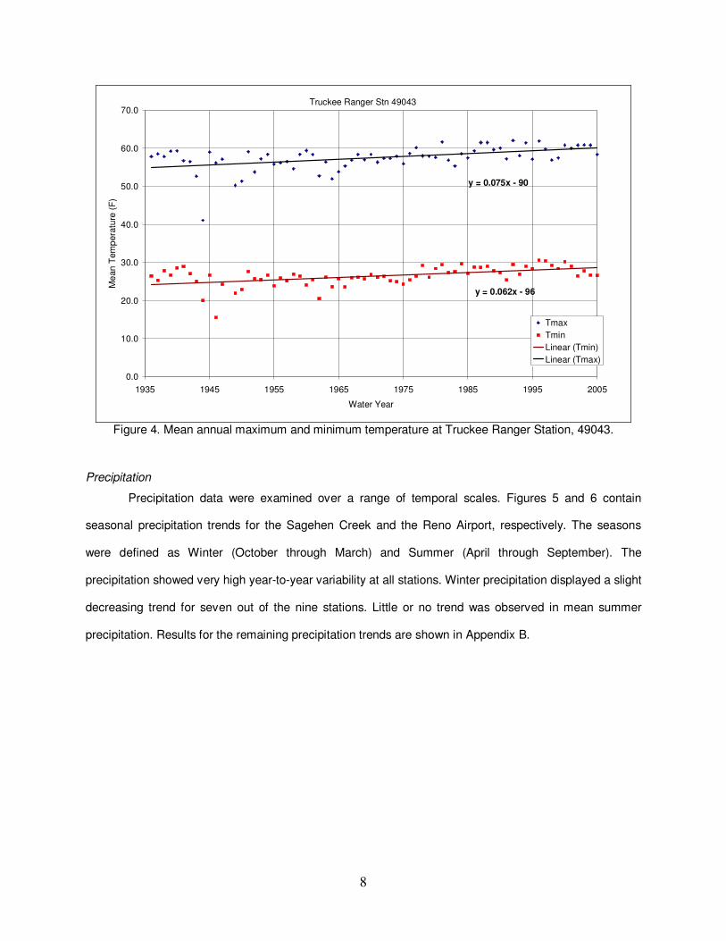
Linear regressions were used to evaluate trends in annual minimum and maximum temperature

at eight weather stations. As an example of the regression results, Figure 4 shows temperature data for

the Truckee Ranger Station. Results for the remaining stations can be found in Appendix A. The data

revealed a slight trend towards increased minimum and maximum temperatures at five gages. However,

three stations showed a trend towards decreased temperatures and year to year variability was quite high

at all stations. The regional temperature trends were overall less than the observed global increase in

surface temperature of approximately 1º F over the past century.

8

Truckee Ranger Stn 49043

y = 0.062x - 96

y = 0.075x - 90

0.0

10.0

20.0

30.0

40.0

50.0

60.0

70.0

1935 1945 1955 1965 1975 1985 1995 2005

Water Year

Me

an T

em

pera

ture

(F

)

Tmax

Tmin

Linear (Tmin)

Linear (Tmax)

Figure 4. Mean annual maximum and minimum temperature at Truckee Ranger Station, 49043.

Precipitation

Precipitation data were examined over a range of temporal scales. Figures 5 and 6 contain

seasonal precipitation trends for the Sagehen Creek and the Reno Airport, respectively. The seasons

were defined as Winter (October through March) and Summer (April through September). The

precipitation showed very high year-to-year variability at all stations. Winter precipitation displayed a slight

decreasing trend for seven out of the nine stations. Little or no trend was observed in mean summer

precipitation. Results for the remaining precipitation trends are shown in Appendix B.

9

Sagehen Creek 47641

y = -0.15x + 330

y = -0.02x + 45

0

10

20

30

40

50

60

1955 1960 1965 1970 1975 1980 1985 1990 1995 2000 2005

Water Year

Me

an

Pre

cip

itatio

n (

in)

Winter

Summer

Linear (Winter)

Linear (Summer)

Figure 5. Mean winter and summer precipitation at Sagehen Creek 47641.

Reno Airport 266779

y = -0.0001x + 5.24

y = 0.0022x - 2.09

0

1

2

3

4

5

6

7

8

9

10

1935 1945 1955 1965 1975 1985 1995 2005

Water Year

Me

an P

recip

itation

(in

)

Winter

Summer

Linear (Winter)

Linear (Summer)

Figure 6. Mean winter and summer precipitation at the Reno Airport 2666779.

10

Snow Water Equivalent

Snow water equivalent (SWE) showed very high variability with some stations reporting a slight

trend towards increased snowpack and others showing reduced snowpack trends. For example, SWE

trends for Independence Creek and Mt. Rose Ski Area snowcourse stations are shown in Figures 7 and

8, respectively. Although SWE trends were very small, and variability was very high, the trends were

highly correlated with instrument elevation. High elevation stations observed increased SWE and the low

elevation stations observed reduced SWE (Figure 9). Although this observation is consistent with

expectations for climate change, further investigations of precipitation and temperature trends in the

Truckee Meadows (discussed above) did not corroborate this hypothesis. For example, high elevation

weather stations did not observe increased precipitation and temperature changes were not correlated

with elevation. The remaining SWE data can be found in Appendix C.

Independence Creek Snowcourse

y = -0.058x + 128

0

5

10

15

20

25

30

35

40

1930 1940 1950 1960 1970 1980 1990 2000 2010

Water Year

Ap

ril 1

SW

E (

in)

Figure 7. Annual April 1st SWE at the Independence Creek snowcourse station.

11

Mt. Rose Snowcourse

y = 0.069x - 101.9

0

10

20

30

40

50

60

70

80

90

1910 1920 1930 1940 1950 1960 1970 1980 1990 2000 2010

Water Year

Ap

ril 1

SW

E (

in)

Figure 8. Annual April 1

st SWE at the Mt Rose Ski Area snowcourse station.

y = 4E-05x - 0.307

R2 = 0.50

-0.12

-0.10

-0.08

-0.06

-0.04

-0.02

0.00

0.02

0.04

0.06

0.08

6000 6250 6500 6750 7000 7250 7500 7750 8000 8250 8500 8750 9000

Water Year

Ap

ril 1 S

WE

(in

)

Figure 9. Trends in April 1 SWE snowcourse data as a function of station elevation.

12

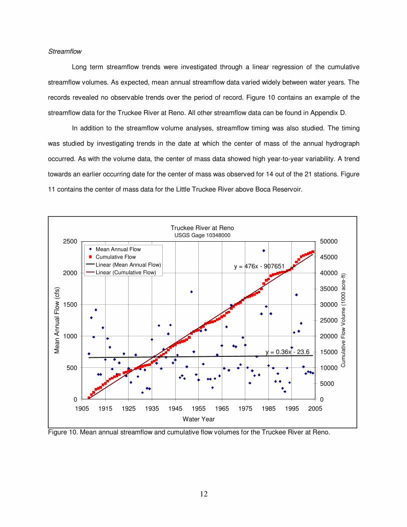
Streamflow

Long term streamflow trends were investigated through a linear regression of the cumulative

streamflow volumes. As expected, mean annual streamflow data varied widely between water years. The

records revealed no observable trends over the period of record. Figure 10 contains an example of the

streamflow data for the Truckee River at Reno. All other streamflow data can be found in Appendix D.

In addition to the streamflow volume analyses, streamflow timing was also studied. The timing

was studied by investigating trends in the date at which the center of mass of the annual hydrograph

occurred. As with the volume data, the center of mass data showed high year-to-year variability. A trend

towards an earlier occurring date for the center of mass was observed for 14 out of the 21 stations. Figure

11 contains the center of mass data for the Little Truckee River above Boca Reservoir.

Truckee River at RenoUSGS Gage 10348000

y = 0.36x - 23.6

y = 476x - 907651

0

500

1000

1500

2000

2500

1905 1915 1925 1935 1945 1955 1965 1975 1985 1995 2005

Water Year

Mean A

nnual F

low

(cfs

)

0

5000

10000

15000

20000

25000

30000

35000

40000

45000

50000

Cu

mu

lative

Flo

w V

olu

me

(1

00

0 a

cre

-ft)

Mean Annual Flow

Cumulative Flow

Linear (Mean Annual Flow)

Linear (Cumulative Flow)

Figure 10. Mean annual streamflow and cumulative flow volumes for the Truckee River at Reno.

13

Little Truckee River above Boca ReservoirUSGS Gage 10344400

y = 0.44x - 666

100

125

150

175

200

225

250

275

1940 1945 1950 1955 1960 1965 1970 1975 1980 1985 1990 1995 2000 2005

Water Year

Ce

nte

r o

f M

ass F

low

Vo

lum

e (

Da

y o

f

Wa

ter

Ye

ar)

Figure 11. Little Truckee River above Boca Reservoir streamflow center of mass.

Reservoir Volumes

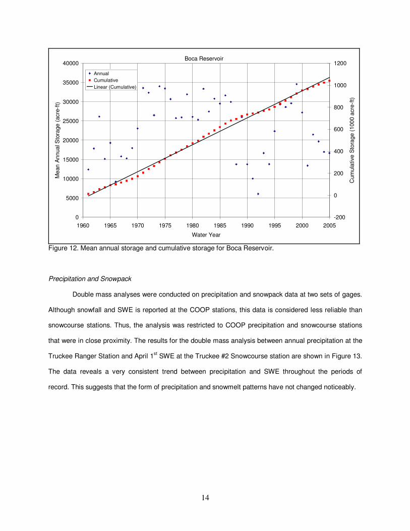
Mean annual reservoir storage volumes and cumulative mean annual storage were also

investigated. The reservoir volumes displayed an obvious dependence on climate, as periods of drought

clearly influenced reservoir volumes. This dependence is demonstrated by Figure 12, which contains data

for Boca Reservoir. In periods of high precipitation and streamflow (e.g. 1972 to 1986), the reservoir

volume was high and the cumulative volume climbed faster than the historical trend. However, during

periods of drought (e.g. 1987 to 1995) the reservoir volumes dropped dramatically, and the cumulative

storage volumes climbed slower than the historical trend. For Lake Tahoe, the storage volume became

negative as the lake level fell below its natural rim. During this period, the cumulative storage volume

trend was actually negative. Lake Tahoe trends, along with the other major regional reservoirs, are shown

in Appendix E.

14

Boca Reservoir

0

5000

10000

15000

20000

25000

30000

35000

40000

1960 1965 1970 1975 1980 1985 1990 1995 2000 2005

Water Year

Me

an

An

nua

l Sto

rage

(acre

-ft)

-200

0

200

400

600

800

1000

1200

Cum

ula

tive

Sto

rag

e (

100

0 a

cre

-ft)

Annual

Cumulative

Linear (Cumulative)

Figure 12. Mean annual storage and cumulative storage for Boca Reservoir.

Precipitation and Snowpack

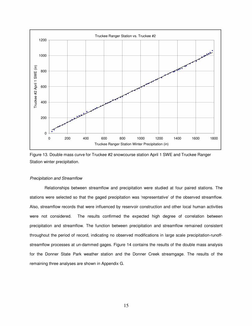
Double mass analyses were conducted on precipitation and snowpack data at two sets of gages.

Although snowfall and SWE is reported at the COOP stations, this data is considered less reliable than

snowcourse stations. Thus, the analysis was restricted to COOP precipitation and snowcourse stations

that were in close proximity. The results for the double mass analysis between annual precipitation at the

Truckee Ranger Station and April 1st SWE at the Truckee #2 Snowcourse station are shown in Figure 13.

The data reveals a very consistent trend between precipitation and SWE throughout the periods of

record. This suggests that the form of precipitation and snowmelt patterns have not changed noticeably.

15

Truckee Ranger Station vs. Truckee #2

0

200

400

600

800

1000

1200

0 200 400 600 800 1000 1200 1400 1600 1800

Truckee Ranger Station Winter Precipitation (in)

Tru

ckee

#2 A

pri

l 1 S

WE

(in

)

Figure 13. Double mass curve for Truckee #2 snowcourse station April 1 SWE and Truckee Ranger

Station winter precipitation.

Precipitation and Streamflow

Relationships between streamflow and precipitation were studied at four paired stations. The

stations were selected so that the gaged precipitation was ‘representative’ of the observed streamflow.

Also, streamflow records that were influenced by reservoir construction and other local human activities

were not considered. The results confirmed the expected high degree of correlation between

precipitation and streamflow. The function between precipitation and streamflow remained consistent

throughout the period of record, indicating no observed modifications in large scale precipitation-runoff-

streamflow processes at un-dammed gages. Figure 14 contains the results of the double mass analysis

for the Donner State Park weather station and the Donner Creek streamgage. The results of the

remaining three analyses are shown in Appendix G.

16

42467 vs. 10338500

0

200

400

600

800

1000

1200

1400

200 400 600 800 1000 1200 1400 1600 1800 2000

Donner State Park Annual Precipitation (in)

Do

nne

r C

ree

k F

low

Vo

lum

e (

10

00

acre

-ft)

Figure 14. Double mass curve for streamflow volume for Donner Creek and annual precipitation at Donner State Park.

Precipitation and Reservoir Storage Volume

Double mass analysis of precipitation and reservoir storage volumes further demonstrated the

high degree of correlation between these variables. The analyses were completed for five paired stations

and the results can be found in Appendix H. An example of this data is shown in Figure 15, which

contains the analyses between Boca Reservoir storage volumes and annual precipitation at the Boca

weather station. The consistent linear long-term trend between these variables indicates that the

underlying processes have not influenced by potential climate change.

17

Boca Reservoir vs. 40931

0

200

400

600

800

1000

1200

0 100 200 300 400 500 600 700 800 900 1000

Boca Gage Annual Precipitation (in)

Bo

ca R

ese

rvoir

(1

00

0 a

cre

-ft)

Figure 15. Double mass curve of Boca Reservoir storage and Boca annual precipitation.

Snow Water Equivalent and Streamflow

Relationships between streamflow and SWE were studied at six paired stations. The stations

were selected so that the gaged SWE was representative of the observed streamflow. Figure 16 shows

the results of the analysis between Independence Lake SWE and Sagehen Creek streamflow. The results

for the remaining analyses can be found in Appendix I. The data showed a high degree of correlation

between SWE and streamflow. Recent data showed no strong departure from long term trends. These

results indicate that the processes of snowfall, snow accumulation, snowmelt, and runoff have remained

relatively consistent throughout the period of record.

18

Independence Lake vs. 10343500

0

50

100

150

200

250

300

350

400

450

0 200 400 600 800 1000 1200 1400 1600 1800 2000 2200

Sagehen Creek Flow Voume (1000 acre-ft)

Ind

epe

nd

ence L

ake

Apri

l 1 S

WE

(in

)

Figure 16. Independence Lake SWE and Sagehen Creek streamflow volumes.

Streamflow and Reservoir Volumes

Double mass analyses were conducted for Boca Reservoir, Donner Lake, Stampede Reservoir

and Lake Tahoe. For Boca Reservoir and Lake Tahoe, inflow and outflow streams were both considered.

Results of the Boca Reservoir Analysis are shown in Figure 17, and all other analyses can be found in

Appendix J. No consistent departures from long term patterns were observed between streamflow and

reservoir volumes. Further, consistent trends were observed between upstream and downstream

streamflow records.

19

10344400 & 10344500 vs. Boca Reservoir

0

1000

2000

3000

4000

5000

6000

0 100 200 300 400 500 600 700 800 900 1000 1100

Boca Reservoir Cumulative Storage (1000 acre-ft)

Little T

ruckee R

iver

Flo

w V

olu

me (

1000 a

cre

-ft)

10344400 (Above)

10344500 (Below)

Linear (10344500 (Below))

Linear (10344400 (Above))

Figure 17. Little Truckee River streamflow volume and Boca Reservoir storage.

Snowpack and Reservoir Storage Volumes

Double mass analysis of April 1 SWE and reservoir storage volumes demonstrated the expected

high degree of correlation between these variables. The analyses were completed for four paired stations

and the results can be found in Appendix K. Figure 18 contains the double mass analysis of Lake Tahoe

storage volume and Hagen’s Meadow April 1 SWE. The data not only reveals the correlation between

these datasets, but it also shows the impacts of major drought events that caused the Lake Tahoe

volume to drop below its natural rim. After these events, SWE continues to accumulate while Lake Tahoe

cumulative storage volumes actually decrease.

20

Lake Tahoe vs. Hagan's Meadow SWE

0

2000

4000

6000

8000

10000

12000

14000

16000

18000

20000

0 100 200 300 400 500 600 700 800

Hagan's Meadow April 1 SWE (in)

La

ke T

ah

oe S

tora

ge (

100

0 a

cre

-ft)

Figure 18. Lake Tahoe storage and April 1 SWE at Hagen’s Meadow snowcourse station.

Summary

In order to reveal potential signs of environmental change in the Truckee Meadows region that

may be consistent and coincident with global warming, historical climate and hydrologic data were

evaluated. The data were compiled in a GIS database and linear regression and double mass analyses

were performed. For all variables, year-to-year variability was very high; making it difficult to identify data

trends. No consistent or prevalent changes in temperature, precipitation, SWE, hydrograph volume/

timing, or reservoir storage volumes were found. Further, relationships between variables appeared to

remain consistent over time. No clear evidence of global warming or associated changes in volume or

timing of hydrologic variables was found.

21

Appendix A

Temperature

22

Boca 40931

y = 0.039x - 16.18

y = 0.022x - 20.07

0

10

20

30

40

50

60

70

1935 1945 1955 1965 1975 1985 1995 2005

Water Year

Me

an

Te

mp

era

ture

(F

)

Tmax

Tmin

Linear (Tmax)

Linear (Tmin)

Figure A1. Mean annual maximum and minimum temperature at Boca Gage 40931.

Donner Park 42467

y = -0.0052x + 68.55

y = 0.0605x - 93.44

0

10

20

30

40

50

60

70

1955 1960 1965 1970 1975 1980 1985 1990 1995 2000 2005

Water Year

Mean T

em

pera

ture

(F

)

Tmax

Tmin

Linear (Tmax)

Linear (Tmin)

Figure A2. Mean annual maximum and minimum temperature at Donner Park 42467.

23

Sagehen Creek 47641

y = 0.011x + 35.0

y = -0.042x + 108.3

0

10

20

30

40

50

60

70

1975 1980 1985 1990 1995 2000 2005

Water Year

Mean T

em

pera

ture

(F

)Tmax

Tmin

Linear (Tmax)

Linear (Tmin)

Figure A3. Mean annual maximum and minimum temperature at Sagehen Creek 47641.

Truckee Ranger Stn 49043

y = 0.062x - 96

y = 0.075x - 90

0.0

10.0

20.0

30.0

40.0

50.0

60.0

70.0

1935 1945 1955 1965 1975 1985 1995 2005

Water Year

Mean T

em

pera

ture

(F

)

Tmax

Tmin

Linear (Tmin)

Linear (Tmax)

Figure A4. Mean annual maximum and minimum temperature at Truckee Ranger Station 49043.

24

Carson City 261485

y = -0.014x + 93.56

y = 0.042x - 49.65

0

10

20

30

40

50

60

70

80

1930 1940 1950 1960 1970 1980 1990 2000 2010

Water Year

Me

an

Tem

pe

ratu

re (

F)

Tmax

Tmin

Linear (Tmax)

Linear (Tmin)

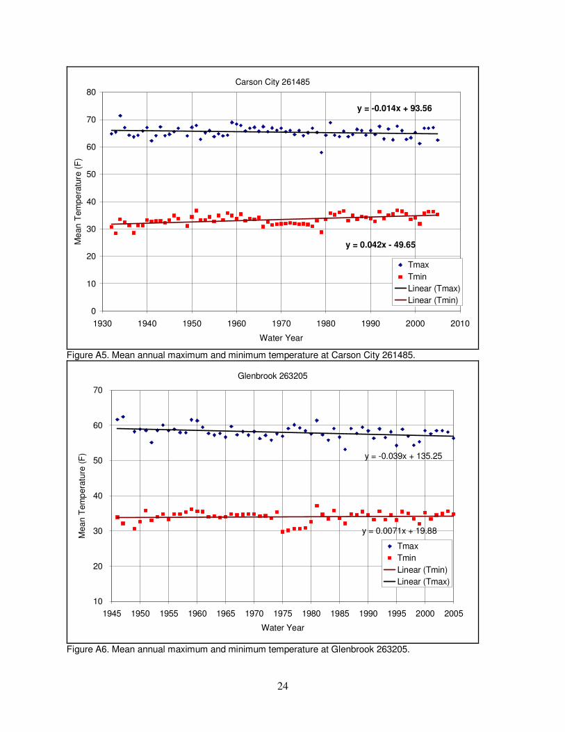
Figure A5. Mean annual maximum and minimum temperature at Carson City 261485.

Glenbrook 263205

y = 0.0071x + 19.88

y = -0.039x + 135.25

10

20

30

40

50

60

70

1945 1950 1955 1960 1965 1970 1975 1980 1985 1990 1995 2000 2005

Water Year

Mean

Tem

pera

ture

(F

)

Tmax

Tmin

Linear (Tmin)

Linear (Tmax)

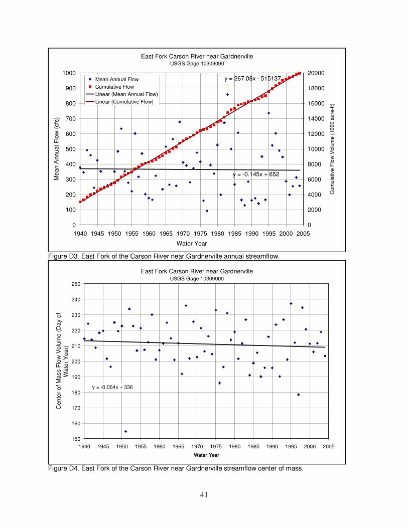
Figure A6. Mean annual maximum and minimum temperature at Glenbrook 263205.

25

Minden 265191

y = 0.0198x + 27.05

y = -0.0229x + 75.85

0

10

20

30

40

50

60

70

80

1930 1940 1950 1960 1970 1980 1990 2000 2010

Water Year

Mean T

em

pe

ratu

re (

F)

Tmax

Tmin

Linear (Tmax)

Linear (Tmin)

Figure A7. Mean annual maximum and minimum temperature at Minden 265191.

Reno Airport 266779

y = 0.008x + 51.0

y = 0.12x - 205.7

0

10

20

30

40

50

60

70

80

1935 1945 1955 1965 1975 1985 1995 2005

Water Year

Mean

Tem

pe

ratu

re (

F)

Tmax

Tmin

Linear (Tmax)

Linear (Tmin)

Figure A8. Mean annual maximum and minimum temperature at Reno Airport!266779.

26

Virginia City 268761

y = 0.137x - 232.7

y = 0.085x - 109.8

20

25

30

35

40

45

50

55

60

65

1955 1960 1965 1970 1975 1980 1985 1990 1995 2000 2005

Water Year

Me

an

Te

mp

era

ture

(F

)

Tmax

Tmin

Linear (Tmin)

Linear (Tmax)

Figure A9. Mean annual maximum and minimum temperature at Virginia City 268761.

27

Appendix B

Precipitation

28

Boca 40931

y = -0.047x + 110.31

y = 0.017x - 29.034

0

5

10

15

20

25

30

35

40

45

1930 1940 1950 1960 1970 1980 1990 2000 2010

Year

Mean P

recip

itation (

in)

Winter

Summer

Linear (Winter)

Linear (Summer)

Figure B1. Mean winter (Oct-March) and summer (April-September) precipitation at Boca Gage 40931.

Donner Park 42467

y = -0.0295x + 90.455

y = -0.009x + 24.78

0

10

20

30

40

50

60

70

80

1955 1960 1965 1970 1975 1980 1985 1990 1995 2000 2005

Water Year

Me

an P

recip

itation (

in)

Winter

Summer

Linear (Winter)

Linear (Summer)

Figure B2. Mean winter and summer precipitation at Donner Park 42467.

29

Sagehen Creek 47641

y = -0.15x + 330

y = -0.02x + 45

0

10

20

30

40

50

60

1955 1960 1965 1970 1975 1980 1985 1990 1995 2000 2005

Water Year

Mean P

recip

itation (

in)

Winter

Summer

Linear (Winter)

Linear (Summer)

Figure B3. Mean winter and summer precipitation at Sagehen Creek 47641.

Truckee Ranger Stn 49043

y = -0.066x + 156.6

y = 0.014x - 21.4

0

5

10

15

20

25

30

35

40

45

50

1935 1945 1955 1965 1975 1985 1995 2005

Water Year

Mea

n P

recip

ita

tion (

in)

Winter

Summer

Linear (Winter)

Linear (Summer)

Figure B4. Mean winter and summer precipitation at Truckee Ranger Station 49043.

30

Carson City 261485

y = -0.040x + 87.45

y = 0.0026x - 2.91

0

2

4

6

8

10

12

14

16

18

20

1930 1940 1950 1960 1970 1980 1990 2000 2010

Water Year

Me

an

Pre

cip

ita

tio

n (

in)

Winter

Summer

Linear (Winter)

Linear (Summer)

Figure B5. Mean winter and summer precipitation at Carson City 261485.

Glenbrook 263205

y = -0.036x + 84.72

y = -0.002x + 8.23

0

5

10

15

20

25

30

35

1945 1955 1965 1975 1985 1995 2005

Water Year

Me

an P

recip

itation (

in)

Winter

Spring

Linear (Winter)

Linear (Spring)

Figure B6. Mean winter and summer precipitation at Glenbrook 263205.

31

Minden 265191

y = -0.0035x + 9.20

y = 0.0007x + 4.92

0

2

4

6

8

10

12

14

1930 1940 1950 1960 1970 1980 1990 2000 2010

Water Year

Me

an

Pre

cip

ita

tion

(in

)Winter

Spring

Linear (Spring)

Linear (Winter)

Figure B7. Mean winter and summer precipitation at Minden 265191.

Reno Airport 266779

y = -0.0001x + 5.24

y = 0.0022x - 2.09

0

1

2

3

4

5

6

7

8

9

10

1935 1945 1955 1965 1975 1985 1995 2005

Water Year

Me

an

Pre

cip

ita

tion

(in

)

Winter

Summer

Linear (Winter)

Linear (Summer)

Figure B8. Mean winter and summer precipitation at the Reno Airport!2666779.

32

Virginia City 268761

y = 0.0549x - 99.349

y = 0.0062x - 9.0298

0

4

8

12

16

20

1950 1955 1960 1965 1970 1975 1980 1985 1990 1995 2000 2005 2010

Water Year

Me

an

Pre

cip

ita

tio

n (

in)

Winter

Summer

Linear (Winter)

Linear (Summer)

Figure B9. Mean winter and summer precipitation at Virginia City 268761.

33

Appendix C

Snowpack

34

Poison Flat Snowcourse

y = 0.0165x - 15.0

0

5

10

15

20

25

30

35

40

45

1940 1950 1960 1970 1980 1990 2000 2010

Water Year

Ap

ril 1

SW

E (

in)

Figure C1. Poison Flat snowcourse station April 1

st SWE.

Blue Lakes Snowcourse

y = -0.0081x + 48

0

10

20

30

40

50

60

70

1900 1920 1940 1960 1980 2000 2020

Water Year

Ap

ril 1 S

WE

(in

)

Figure C2. Blue Lakes snowcourse station April 1

st SWE.

35

Hagan's Meadow Snowcourse

y = -0.014x + 43.3

0

5

10

15

20

25

30

35

40

45

1910 1920 1930 1940 1950 1960 1970 1980 1990 2000 2010

Water Year

April 1 S

WE

(in

)

Figure C3. Hagan’s Meadow snowcourse station April 1

st SWE.

Independence Creek Snowcourse

y = -0.058x + 128

0

5

10

15

20

25

30

35

40

1930 1940 1950 1960 1970 1980 1990 2000 2010

Water Year

April 1 S

WE

(in

)

Figure C4. Independence Creek snowcourse station April 1

st SWE.

36

Independence Camp Snowcourse

y = -0.108x + 233

0

10

20

30

40

50

60

70

1940 1950 1960 1970 1980 1990 2000 2010

Water Year

April 1 S

WE

(in

)

Figure C5. Independence Camp snowcourse station April 1

st SWE.

Independence Lake Snowcourse

y = 0.031x - 19.8

0

10

20

30

40

50

60

70

80

90

1935 1945 1955 1965 1975 1985 1995 2005

Water Year

April 1 S

WE

(in

)

Figure C6. Independence Lake snowcourse station April 1

st SWE.

37

Rubicon #2 Snowcourse

y = 0.0204x - 11.4

0

10

20

30

40

50

60

70

1910 1920 1930 1940 1950 1960 1970 1980 1990 2000 2010

Water Year

Ap

ril 1

SW

E (

in)

Figure C7. Rubicon #2 snowcourse station April 1

st SWE.

Truckee #2 Snowcourse

y = -0.031x + 76.5

0

5

10

15

20

25

30

35

40

1930 1940 1950 1960 1970 1980 1990 2000 2010

Water Year

Ap

ril 1

SW

E (

in)

Figure C8. Truckee #2 snowcourse station April 1

st SWE.

38

Marlette Snowcourse

y = -0.0002x + 24.3

0

10

20

30

40

50

60

1910 1920 1930 1940 1950 1960 1970 1980 1990 2000 2010

Water Year

Ap

ril 1

SW

E (

in)

Figure C9. Marlette Lake snowcourse station April 1

st SWE.

Mt. Rose Snowcourse

y = 0.069x - 101.9

0

10

20

30

40

50

60

70

80

90

1910 1920 1930 1940 1950 1960 1970 1980 1990 2000 2010

Water Year

Ap

ril 1

SW

E (

in)

Figure C10. Mt Rose Ski Area snowcourse station April 1

st SWE.

39

Appendix D

Streamflow

40

East Fork Carson River near Markleeville

USGS Gage 10308200

y = -0.5056x + 1358

y = 263.69x - 516903

0

100

200

300

400

500

600

700

800

900

1960 1965 1970 1975 1980 1985 1990 1995 2000 2005

Water Year

Me

an

Ann

ua

l F

low

(cfs

)

0

2000

4000

6000

8000

10000

12000

Cum

ula

tive F

low

Volu

me (

10

00 a

cre

-ft)

Mean Annual Flow

Cumulative Flow

Linear (Mean Annual Flow)

Linear (Cumulative Flow)

Figure D1. East Fork of the Carson River near Markleeville annual streamflow.

East Fork Carson River near MarkleevilleUSGS Gage 1030900

y = -0.028x + 267

150

160

170

180

190

200

210

220

230

240

250

1960 1965 1970 1975 1980 1985 1990 1995 2000 2005

Water Year

Ce

nte

r o

f M

ass F

low

Vo

lum

e (

Da

y o

f

Wa

ter

Ye

ar)

Figure D2. East Fork of the Carson River near Markleeville streamflow center of mass.

41

East Fork Carson River near GardnervilleUSGS Gage 10309000

y = -0.145x + 652

y = 267.08x - 515137

0

100

200

300

400

500

600

700

800

900

1000

1940 1945 1950 1955 1960 1965 1970 1975 1980 1985 1990 1995 2000 2005

Water Year

Me

an

Ann

ua

l F

low

(cfs

)

0

2000

4000

6000

8000

10000

12000

14000

16000

18000

20000

Cum

ula

tive F

low

Volu

me (

10

00 a

cre

-ft)

Mean Annual Flow

Cumulative Flow

Linear (Mean Annual Flow)

Linear (Cumulative Flow)

Figure D3. East Fork of the Carson River near Gardnerville annual streamflow.

East Fork Carson River near GardnervilleUSGS Gage 10309000

y = -0.064x + 336

150

160

170

180

190

200

210

220

230

240

250

1940 1945 1950 1955 1960 1965 1970 1975 1980 1985 1990 1995 2000 2005

Water Year

Cen

ter

of M

ass F

low

Vo

lum

e (

Day o

f

Wate

r Y

ea

r)

Figure D4. East Fork of the Carson River near Gardnerville streamflow center of mass.

42

West Fork Carson River near Woodsfords

USGS Gage 10310000

y = 0.008x + 89

y = 76.2x - 145121

0

25

50

75

100

125

150

175

200

225

250

1940 1945 1950 1955 1960 1965 1970 1975 1980 1985 1990 1995 2000 2005

Water Year

Me

an

Ann

ua

l F

low

(cfs

)

2000

3000

4000

5000

6000

7000

8000

Cum

ula

tive F

low

Volu

me (

10

00 a

cre

-ft)

Mean Annual Flow

Cumulative Flow

Linear (Mean Annual Flow)

Linear (Cumulative Flow)

Figure D5. West Fork of the Carson River near Woodsford annual streamflow.

West Fork Carson River near WoodsfordsUSGS Gage 10310000

y = -0.079x + 366

150

160

170

180

190

200

210

220

230

240

250

1940 1945 1950 1955 1960 1965 1970 1975 1980 1985 1990 1995 2000 2005

Water Year

Ce

nte

r o

f M

ass F

low

Vo

lum

e (

Da

y o

f

Wa

ter

Ye

ar)

Figure D6. West Fork of the Carson River near Woodsford streamflow center of mass.

43

Carson River near Carson CityUSGS Gage 1031100

y = -0.066x + 536

y = 297x - 576709

0

200

400

600

800

1000

1200

1940 1945 1950 1955 1960 1965 1970 1975 1980 1985 1990 1995 2000 2005

Water Year

Mean

An

nual F

low

(cfs

)

0

2000

4000

6000

8000

10000

12000

14000

16000

18000

20000

Cu

mu

lative

Flo

w V

olu

me

(1

000

acre

-ft)

Mean Annual Flow

Cumulative Flow

Linear (Mean Annual Flow)

Linear (Cumulative Flow)

Figure D7. Carson River near Carson City annual streamflow.

Carson River near Carson CityUSGS Gage 1031100

y = -0.1561x + 496.01

100

125

150

175

200

225

250

1940 1945 1950 1955 1960 1965 1970 1975 1980 1985 1990 1995 2000 2005

Water Year

Cen

ter

of M

ass F

low

Vo

lum

e (

Da

y o

f

Wate

r Y

ea

r)

Figure D8. Carson River near Carson City streamflow center of mass.

44

Blackwood Creek near Tahoe CityUSGS Gage 10336660

y = -0.156x + 346

y = 216x - 414095

0

10

20

30

40

50

60

70

80

1960 1965 1970 1975 1980 1985 1990 1995 2000 2005

Water Year

Mean

An

nual F

low

(cfs

)

0

200

400

600

800

1000

1200

Cu

mu

lative

Flo

w V

olu

me

(1

000

acre

-ft)

Mean Annual Flow

Cumulative Flow

Linear (Mean Annual Flow)

Linear (Cumulative Flow)

Figure D9. Blackwood Creek near Tahoe City annual streamflow.

Blackwood Creek near Tahoe CityUSGS Gage 10336660

y = 0.17x - 127

150

160

170

180

190

200

210

220

230

240

250

1960 1965 1970 1975 1980 1985 1990 1995 2000 2005

Water Year

Cen

ter

of M

ass F

low

Vo

lum

e (

Da

y o

f

Wate

r Y

ea

r)

Figure D10. Blackwood Creek near Tahoe City streamflow center of mass.

45

Third Creek near Crystal BayUSGS Gage 10336698

y = -0.043x + 93

y = 6.84x - 13455

0

4

8

12

16

20

1970 1975 1980 1985 1990 1995 2000 2005

Water Year

Mean

An

nual F

low

(cfs

)

0

50

100

150

200

250

300

Cu

mu

lative

Flo

w V

olu

me

(1

000

acre

-ft)

Mean Annual Flow

Cumulative Flow

Linear (Mean Annual Flow)

Linear (Cumulative Flow)

Figure D11. Third Creek near Crystal Bay annual streamflow.

Third Creek near Crystal BayUSGS Gage 10336698

y = -0.380x + 959

150

160

170

180

190

200

210

220

230

240

250

1970 1975 1980 1985 1990 1995 2000 2005

Water Year

Cen

ter

of M

ass F

low

Vo

lum

e (

Da

y o

f

Wate

r Y

ea

r)

Figure D12. Third Creek near Crystal Bay streamflow center of mass.

46

Incline Creek near Crystal BayUSGS Gage 10336700

y = -0.010x + 28

y = 6.86x - 13497

0

2

4

6

8

10

12

14

1970 1975 1980 1985 1990 1995 2000 2005

Water Year

Mean

An

nual F

low

(cfs

)

0

25

50

75

100

125

150

175

200

225

250

Cu

mu

lative

Flo

w V

olu

me

(1

000

acre

-ft)

Mean Annual Flow

Cumulative Flow

Linear (Mean Annual Flow)

Linear (Cumulative Flow)

Figure D13. Incline Creek near Crystal Bay annual streamflow.

Incline Creek near Crystal BayUSGS Gage 10336700

y = -0.177x + 548

150

160

170

180

190

200

210

220

230

240

250

1975 1980 1985 1990 1995 2000 2005

Water Year

Cen

ter

of M

ass F

low

Vo

lum

e (

Da

y o

f

Wate

r Y

ea

r)

Figure D14. Incline Creek near Crystal Bay streamflow center of mass.

47

Trout Creek near Tahoe ValleyUSGS Gage 10336780

y = -0.05x + 135

y = 27.0x - 53024

0

10

20

30

40

50

60

70

80

90

1960 1965 1970 1975 1980 1985 1990 1995 2000 2005

Water Year

Mean

An

nual F

low

(cfs

)

0

200

400

600

800

1000

1200

Cu

mu

lative

Flo

w V

olu

me

(1

000

acre

-ft)

Mean Annual Flow

Cumulative Flow

Linear (Mean Annual Flow)

Linear (Cumulative Flow)

Figure D15. Trout Creek near Tahoe Valley annual streamflow.

Trout Creek near Tahoe ValleyUSGS Gage 10336780

y = -0.063x + 324

150

160

170

180

190

200

210

220

230

240

250

1960 1965 1970 1975 1980 1985 1990 1995 2000 2005

Water Year

Cen

ter

of M

ass F

low

Vo

lum

e (

Da

y o

f

Wate

r Y

ea

r)

Figure D16. Trout Creek near Tahoe Valley streamflow center of mass.

48

Truckee River at Tahoe CityUSGS Gage 10337500

y = 0.18x - 125

y = 166x - 317204

0

100

200

300

400

500

600

700

800

1910 1920 1930 1940 1950 1960 1970 1980 1990 2000 2010

Water Year

Mean

An

nual F

low

(cfs

)

0

2000

4000

6000

8000

10000

12000

14000

16000

Cu

mu

lative

Flo

w V

olu

me

(1

000

acre

-ft)

Mean Annual Flow

Cumulative Flow

Linear (Mean Annual Flow)

Linear (Cumulative Flow)

Figure D17. Truckee River at Tahoe City annual streamflow.

Truckee River at Tahoe CityUSGS Gage 10337500

y = 0.098x + 14

150

160

170

180

190

200

210

220

230

240

250

1910 1920 1930 1940 1950 1960 1970 1980 1990 2000 2010

Water Year

Cen

ter

of M

ass F

low

Vo

lum

e (

Da

y o

f

Wate

r Y

ea

r)

Figure D18. Truckee River at Tahoe City streamflow center of mass.

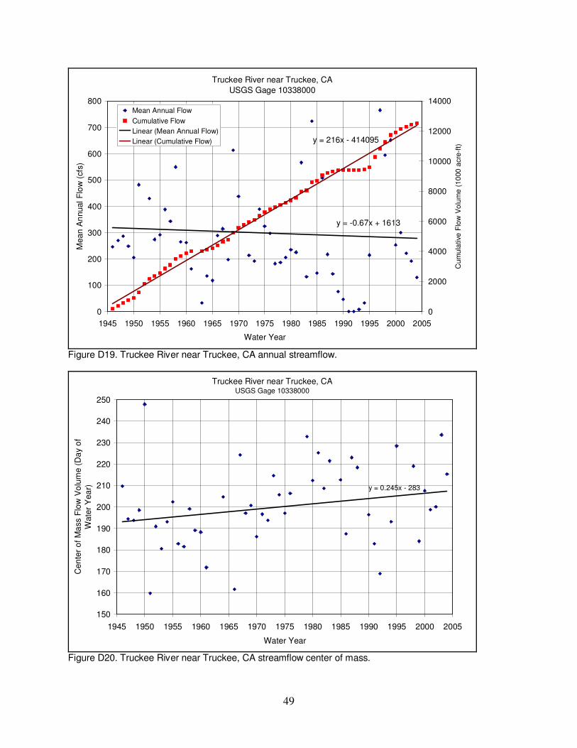
49

Truckee River near Truckee, CA

USGS Gage 10338000

y = -0.67x + 1613

y = 216x - 414095

0

100

200

300

400

500

600

700

800

1945 1950 1955 1960 1965 1970 1975 1980 1985 1990 1995 2000 2005

Water Year

Mean

An

nual F

low

(cfs

)

0

2000

4000

6000

8000

10000

12000

14000

Cu

mu

lative

Flo

w V

olu

me

(1

000

acre

-ft)

Mean Annual Flow

Cumulative Flow

Linear (Mean Annual Flow)

Linear (Cumulative Flow)

Figure D19. Truckee River near Truckee, CA annual streamflow.

Truckee River near Truckee, CAUSGS Gage 10338000

y = 0.245x - 283

150

160

170

180

190

200

210

220

230

240

250

1945 1950 1955 1960 1965 1970 1975 1980 1985 1990 1995 2000 2005

Water Year

Cen

ter

of M

ass F

low

Vo

lum

e (

Da

y o

f

Wate

r Y

ea

r)

Figure D20. Truckee River near Truckee, CA streamflow center of mass.

50

Donner Creek near Truckee, CAUSGS Gage 10338500

y = 0.0016x + 34

y = 28x - 54859

0

10

20

30

40

50

60

70

80

90

100

1955 1960 1965 1970 1975 1980 1985 1990 1995 2000 2005

Water Year

Mean

An

nual F

low

(cfs

)

0

200

400

600

800

1000

1200

1400

Cu

mu

lative

Flo

w V

olu

me

(1

000

acre

-ft)

Mean Annual Flow

Cumulative Flow

Linear (Mean Annual Flow)

Linear (Cumulative Flow)

Figure D21. Donner Creek near Truckee, CA annual streamflow.

Donner Creek near Truckee, CAUSGS Gage 10338500

y = 0.14x - 105

150

160

170

180

190

200

210

220

1955 1960 1965 1970 1975 1980 1985 1990 1995 2000 2005

Water Year

Cen

ter

of M

ass F

low

Vo

lum

e (

Da

y o

f

Wate

r Y

ea

r)

Figure D22. Donner Creek near Truckee, CA streamflow center of mass.

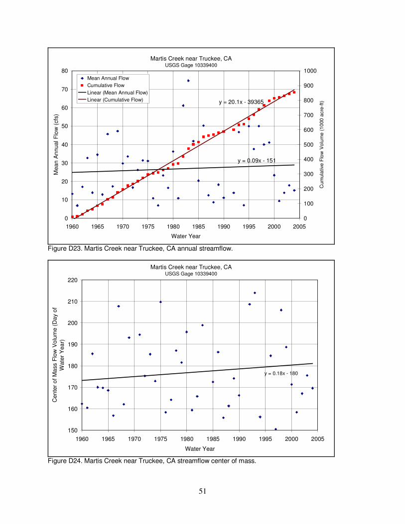
51

Martis Creek near Truckee, CAUSGS Gage 10339400

y = 0.09x - 151

y = 20.1x - 39365

0

10

20

30

40

50

60

70

80

1960 1965 1970 1975 1980 1985 1990 1995 2000 2005

Water Year

Mean

An

nual F

low

(cfs

)

0

100

200

300

400

500

600

700

800

900

1000

Cu

mu

lative

Flo

w V

olu

me

(1

000

acre

-ft)

Mean Annual Flow

Cumulative Flow

Linear (Mean Annual Flow)

Linear (Cumulative Flow)

Figure D23. Martis Creek near Truckee, CA annual streamflow.

Martis Creek near Truckee, CAUSGS Gage 10339400

y = 0.18x - 180

150

160

170

180

190

200

210

220

1960 1965 1970 1975 1980 1985 1990 1995 2000 2005

Water Year

Cen

ter

of M

ass F

low

Vo

lum

e (

Da

y o

f

Wate

r Y

ea

r)

Figure D24. Martis Creek near Truckee, CA streamflow center of mass.

52

Prosser Creek near Prosser DamUSGS Gage 10340500

y = 0.15x - 214

y = 64.8x - 125996

0

25

50

75

100

125

150

175

200

225

250

1940 1945 1950 1955 1960 1965 1970 1975 1980 1985 1990 1995 2000 2005

Water Year

Mean

An

nual F

low

(cfs

)

0

500

1000

1500

2000

2500

3000

3500

4000

Cu

mu

lative

Flo

w V

olu

me

(1

000

acre

-ft)

Mean Annual Flow

Cumulative Flow

Linear (Mean Annual Flow)

Linear (Cumulative Flow)

Figure D25. Prosser Creek near Prosser Dam annual streamflow.

Prosser Creek near Prosser DamUSGS Gage 10340500

y = -0.087x + 367

150

160

170

180

190

200

210

220

230

240

250

1940 1945 1950 1955 1960 1965 1970 1975 1980 1985 1990 1995 2000 2005

Water Year

Cen

ter

of M

ass F

low

Vo

lum

e (

Da

y o

f

Wate

r Y

ea

r)

Figure D26. Prosser Creek near Prosser Dam streamflow center of mass.

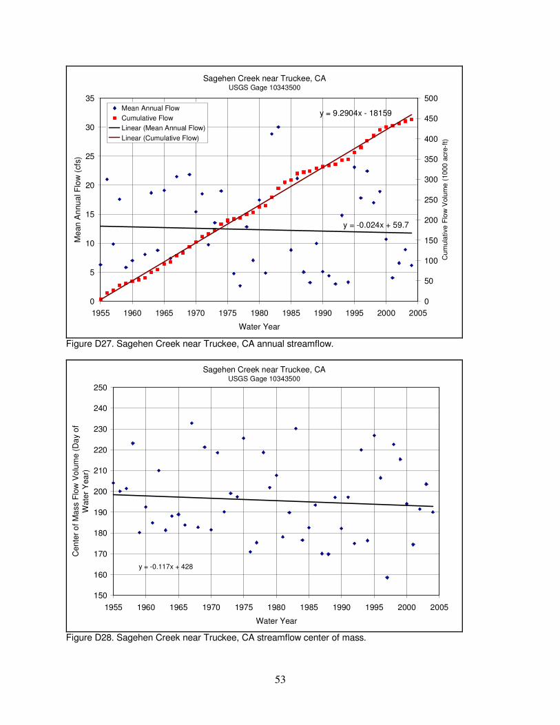
53

Sagehen Creek near Truckee, CAUSGS Gage 10343500

y = -0.024x + 59.7

y = 9.2904x - 18159

0

5

10

15

20

25

30

35

1955 1960 1965 1970 1975 1980 1985 1990 1995 2000 2005

Water Year

Me

an

An

nu

al F

low

(cfs

)

0

50

100

150

200

250

300

350

400

450

500

Cum

ula

tive

Flo

w V

olu

me

(10

00

acre

-ft)

Mean Annual Flow

Cumulative Flow

Linear (Mean Annual Flow)

Linear (Cumulative Flow)

Figure D27. Sagehen Creek near Truckee, CA annual streamflow.

Sagehen Creek near Truckee, CAUSGS Gage 10343500

y = -0.117x + 428

150

160

170

180

190

200

210

220

230

240

250

1955 1960 1965 1970 1975 1980 1985 1990 1995 2000 2005

Water Year

Cen

ter

of M

ass F

low

Vo

lum

e (

Da

y o

f

Wate

r Y

ea

r)

Figure D28. Sagehen Creek near Truckee, CA streamflow center of mass.

54

Little Truckee River above Boca ReservoirUSGS Gage 10344400

y = 0.0149x + 136.9

y = 122.75x - 238096

0

50

100

150

200

250

300

350

400

450

1940 1945 1950 1955 1960 1965 1970 1975 1980 1985 1990 1995 2000 2005

Water Year

Mean

An

nual F

low

(cfs

)

0

1000

2000

3000

4000

5000

6000

7000

8000

Cu

mu

lative

Flo

w V

olu

me

(1

000

acre

-ft)

Mean Annual Flow

Cumulative Flow

Linear (Mean Annual Flow)

Linear (Cumulative Flow)

Figure D29. Little Truckee River above Boca Reservoir annual streamflow.

Little Truckee River above Boca ReservoirUSGS Gage 10344400

y = 0.44x - 666

100

125

150

175

200

225

250

275

1940 1945 1950 1955 1960 1965 1970 1975 1980 1985 1990 1995 2000 2005

Water Year

Cen

ter

of M

ass F

low

Vo

lum

e (

Da

y o

f

Wate

r Y

ea

r)

Figure D30. Little Truckee River above Boca Reservoir streamflow center of mass.

55

Little Truckee River below Boca ReservoirUSGS Gage 10344500

y = 0.22x - 259

y = 120x - 229741

0

50

100

150

200

250

300

350

400

450

500

1910 1920 1930 1940 1950 1960 1970 1980 1990 2000 2010

Water Year

Mean

An

nual F

low

(cfs

)

0

2000

4000

6000

8000

10000

12000

Cu

mu

lative

Flo

w V

olu

me

(1

000

acre

-ft)

Mean Annual Flow

Cumulative Flow

Linear (Mean Annual Flow)

Linear (Cumulative Flow)

Figure D31. Little Truckee River below Boca Reservoir annual streamflow.

Little Truckee River below Boca ReservoirUSGS Gage 10344500

y = 0.056x + 96.2

100

125

150

175

200

225

250

275

300

325

1910 1920 1930 1940 1950 1960 1970 1980 1990 2000 2010

Water Year

Cen

ter

of M

ass F

low

Vo

lum

e (

Da

y o

f

Wate

r Y

ea

r)

Figure D32. Little Truckee River below Boca Reservoir streamflow center of mass.

56

Truckee River at FaradUSGS Gage 10346000

y = 0.91x - 1013

y = 550x - 1E+06

0

250

500

750

1000

1250

1500

1750

2000

2250

2500

1910 1920 1930 1940 1950 1960 1970 1980 1990 2000 2010

Water Year

Me

an

An

nu

al F

low

(cfs

)

0

10000

20000

30000

40000

50000

60000

Cum

ula

tive

Flo

w V

olu

me

(10

00

acre

-ft)

Mean Annual Flow

Cumulative Flow

Linear (Mean Annual Flow)

Linear (Cumulative Flow)

Figure D33. Truckee River at Farad annual streamflow.

Truckee River at FaradUSGS Gage 10346000

y = -0.017x + 233.

100

120

140

160

180

200

220

240

260

1910 1920 1930 1940 1950 1960 1970 1980 1990 2000 2010

Water Year

Cen

ter

of M

ass F

low

Vo

lum

e (

Da

y o

f

Wate

r Y

ea

r)

Figure D34. Truckee River at Farad streamflow center of mass.

57

Hunter Creek near RenoUSGS Gage 10347600

y = 20x - 39074

y = 444x - 874580

0

500

1000

1500

2000

2500

3000

1960 1965 1970 1975 1980 1985 1990 1995 2000 2005

Water Year

Mean

An

nual F

low

(cfs

)

0

2000

4000

6000

8000

10000

12000

14000

16000

18000

Cu

mu

lative

Flo

w V

olu

me

(1

000

acre

-ft)

Mean Annual Flow

Cumulative Flow

Linear (Mean Annual Flow)

Linear (Cumulative Flow)

Figure D35. Hunter Creek near Reno annual streamflow.

Hunter Creek near RenoUSGS Gage 10347600

y = -0.11x + 417

150

160

170

180

190

200

210

220

230

240

1960 1965 1970 1975 1980 1985 1990 1995 2000 2005

Water Year

Cen

ter

of M

ass F

low

Vo

lum

e (

Da

y o

f

Wate

r Y

ea

r)

Figure D36. Hunter Creek near Reno streamflow center of mass.

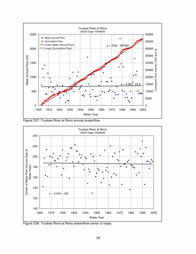
58

Truckee River at RenoUSGS Gage 10348000

y = 0.36x - 23.6

y = 476x - 907651

0

500

1000

1500

2000

2500

1905 1915 1925 1935 1945 1955 1965 1975 1985 1995 2005

Water Year

Me

an

An

nu

al F

low

(cfs

)

0

5000

10000

15000

20000

25000

30000

35000

40000

45000

50000

Cum

ula

tive

Flo

w V

olu

me

(10

00

acre

-ft)

Mean Annual Flow

Cumulative Flow

Linear (Mean Annual Flow)

Linear (Cumulative Flow)

Figure D37. Truckee River at Reno annual streamflow.

Truckee River at RenoUSGS Gage 10348000

y = -0.022x + 229

100

120

140

160

180

200

220

240

1905 1915 1925 1935 1945 1955 1965 1975 1985 1995 2005

Water Year

Cen

ter

of M

ass F

low

Vo

lum

e (

Da

y o

f

Wate

r Y

ea

r)

Figure D38. Truckee River at Reno streamflow center of mass.

59

Steamboat Creek at Steamboat, NVUSGS Gage 10349300

y = 0.14x - 258

y = 16x - 31497

0

10

20

30

40

50

60

70

80

90

100

1960 1965 1970 1975 1980 1985 1990 1995 2000 2005

Water Year

Mean

An

nua

l F

low

(cfs

)

0

100

200

300

400

500

600

700

Cu

mu

lative

Flo

w V

olu

me

(1

000

acre

-ft)

Mean Annual Flow

Cumulative Flow

Linear (Mean Annual Flow)

Linear (Cumulative Flow)

Figure D39. Steamboat Creek at Steamboat, NV annual streamflow.

Steamboat Creek at Steamboat, NVUSGS Gage 10349300

y = -0.43x + 1033

100

125

150

175

200

225

250

1960 1965 1970 1975 1980 1985 1990 1995 2000 2005

Water Year

Cen

ter

of M

ass F

low

Vo

lum

e (

Da

y o

f

Wate

r Y

ea

r)

Figure D40. Steamboat Creek at Steamboat, NV streamflow center of mass.

60

Truckee River at VistaUSGS Gage 10350000

y = -0.0619x + 898.29

y = 523x - 993224

0

200

400

600

800

1000

1200

1400

1600

1800

2000

1900 1910 1920 1930 1940 1950 1960 1970 1980 1990 2000 2010

Water Year

Me

an

An

nu

al F

low

(cfs

)

0

10000

20000

30000

40000

50000

60000

Cum

ula

tive

Flo

w V

olu

me

(10

00

acre

-ft)

Mean Annual Flow

Cumulative Flow

Linear (Mean Annual Flow)

Linear (Cumulative Flow)

Figure D41. Truckee River at Vista annual streamflow.

Truckee River at VistaUSGS Gage 10350000

y = -0.076x + 333

100

120

140

160

180

200

220

240

1900 1910 1920 1930 1940 1950 1960 1970 1980 1990 2000 2010

Water Year

Cen

ter

of M

ass F

low

Vo

lum

e (

Da

y o

f

Wate

r Y

ea

r)

Figure D42. Truckee River at Vista streamflow center of mass.

61

Appendix E

Reservoir Volumes

62

Boca Reservoir

0

5000

10000

15000

20000

25000

30000

35000

40000

1960 1965 1970 1975 1980 1985 1990 1995 2000 2005

Water Year

Mean

Annu

al S

tora

ge

(acre

-ft)

-200

0

200

400

600

800

1000

1200

Cum

ula

tive S

tora

ge (

10

00 a

cre

-ft)

Annual

Cumulative

Linear (Cumulative)

Figure E1. Mean annual storage and cumulative storage for Boca Reservoir.

Donner Lake

0

1000

2000

3000

4000

5000

6000

7000

1990 1992 1994 1996 1998 2000 2002 2004 2006

Water Year

Mean

Annu

al S

tora

ge

(acre

-ft)

0

10

20

30

40

50

60

70

80

90

100

Cum

ula

tive S

tora

ge (

10

00 a

cre

-ft)

Anual

Cumulative

Linear (Cumulative)

Figure E2. Mean annual storage and cumulative storage for Donner Lake.

63

Independence Lake

0

2000

4000

6000

8000

10000

12000

14000

16000

18000

1990 1992 1994 1996 1998 2000 2002 2004 2006

Water Year

Mean

Annu

al S

tora

ge

(acre

-ft)

0

50

100

150

200

250

Cum

ula

tive S

tora

ge (

10

00 a

cre

-ft)

Annual

Cumulative

Linear (Cumulative)

Figure E3. Mean annual storage and cumulative storage for Independence Lake.

Lahontan Reservoir

0

50000

100000

150000

200000

250000

300000

1915 1925 1935 1945 1955 1965 1975 1985 1995 2005

Water Year

Mean

Annu

al S

tora

ge

(acre

-ft)

-2000

0

2000

4000

6000

8000

10000

12000

14000

16000

Cum

ula

tive S

tora

ge (

10

00 a

cre

-ft)

Annual

Cumulative

Linear (Cumulative)

Figure E4. Mean annual storage and cumulative storage for Lahontan Reservoir.

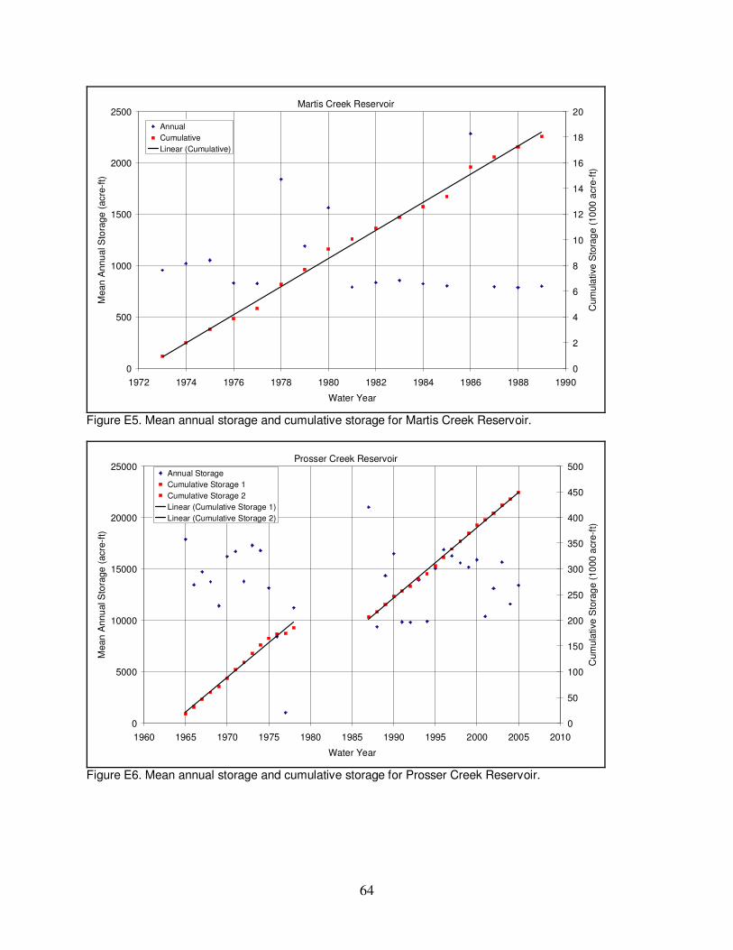
64

Martis Creek Reservoir

0

500

1000

1500

2000

2500

1972 1974 1976 1978 1980 1982 1984 1986 1988 1990

Water Year

Mean

Annu

al S

tora

ge

(acre

-ft)

0

2

4

6

8

10

12

14

16

18

20

Cum

ula

tive S

tora

ge (

10

00 a

cre

-ft)

Annual

Cumulative

Linear (Cumulative)

Figure E5. Mean annual storage and cumulative storage for Martis Creek Reservoir.

Prosser Creek Reservoir

0

5000

10000

15000

20000

25000

1960 1965 1970 1975 1980 1985 1990 1995 2000 2005 2010

Water Year

Mean

Annu

al S

tora

ge

(acre

-ft)

0

50

100

150

200

250

300

350

400

450

500

Cum

ula

tive S

tora

ge (

10

00 a

cre

-ft)

Annual Storage

Cumulative Storage 1

Cumulative Storage 2

Linear (Cumulative Storage 1)

Linear (Cumulative Storage 2)

Figure E6. Mean annual storage and cumulative storage for Prosser Creek Reservoir.

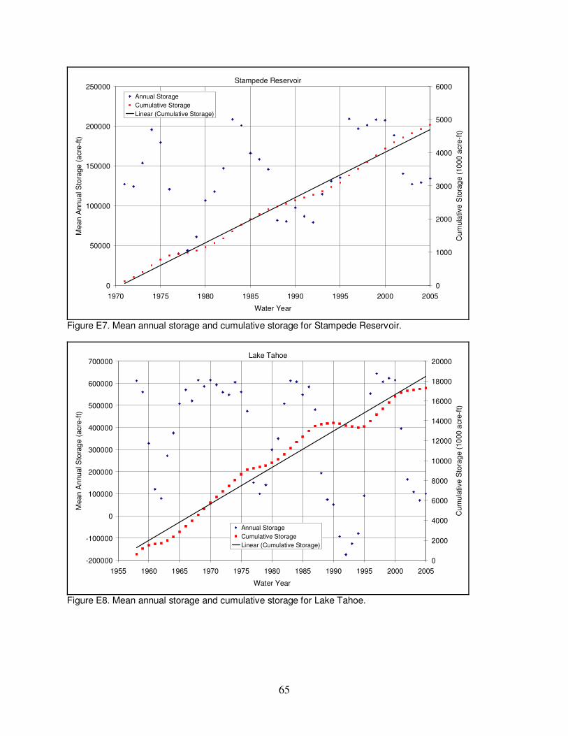
65

Stampede Reservoir

0

50000

100000

150000

200000

250000

1970 1975 1980 1985 1990 1995 2000 2005

Water Year

Mean

Annu

al S

tora

ge

(acre

-ft)

0

1000

2000

3000

4000

5000

6000

Cum

ula

tive S

tora

ge (

10

00 a

cre

-ft)

Annual Storage

Cumulative Storage

Linear (Cumulative Storage)

Figure E7. Mean annual storage and cumulative storage for Stampede Reservoir.

Lake Tahoe

-200000

-100000

0

100000

200000

300000

400000

500000

600000

700000

1955 1960 1965 1970 1975 1980 1985 1990 1995 2000 2005

Water Year

Mean

Annu

al S

tora

ge

(acre

-ft)

0

2000

4000

6000

8000

10000

12000

14000

16000

18000

20000

Cum

ula

tive S

tora

ge (

10

00 a

cre

-ft)

Annual Storage

Cumulative Storage

Linear (Cumulative Storage)

Figure E8. Mean annual storage and cumulative storage for Lake Tahoe.

66

Appendix F

Double Mass Curve Analysis Precipitation and Snowpack

67

Sagehen Creek vs. Independence Lake

0

500

1000

1500

2000

2500

0 200 400 600 800 1000 1200 1400

Sagehen Creek Winter Precipitation (in)

Indep

ende

nce

Lake A

pri

l 1 S

WE

(in

)

Figure F1. Double mass curve for Independence Lake snowcourse station April 1 SWE and Sagehen Creek winter precipitation.

Truckee Ranger Station vs. Truckee #2

0

200

400

600

800

1000

1200

0 200 400 600 800 1000 1200 1400 1600 1800

Truckee Ranger Station Winter Precipitation (in)

Tru

ckee #

2 A

pri

l 1 S

WE

(in

)

Figure F2. Double mass curve for Truckee #2 snowcourse station April 1 SWE and Truckee Ranger Station winter precipitation.

68

Appendix G

Double Mass Curve Analysis Precipitation vs. Streamflow

69

42467 vs. 10338500

0

200

400

600

800

1000

1200

1400

200 400 600 800 1000 1200 1400 1600 1800 2000

Donner State Park Annual Precipitation (in)

Do

nner

Cre

ek F

low

Volu

me (

1000

acre

-ft)

Figure G1. Double mass curve for streamflow volume for Donner Creek and annual precipitation at Donner State Park.

47641 vs. 10343500

0

50

100

150

200

250

300

350

400

450

500

0 200 400 600 800 1000 1200 1400 1600 1800

Sagehen Creek Annual Precipitation (in)

Sage

hen

Cre

ek F

low

Volu

me (

100

0 a

cre

-ft)

Figure G2. Double mass curve for Sagehen Creek streamflow volume and annual precipitation at the Sagehen weather station.

70

49043 vs. 10339400

0

100

200

300

400

500

600

700

800

900

1000

0 100 200 300 400 500 600 700 800 900 1000 1100 1200 1300 1400 1500

Truckee Ranger Stn Annual Precipitation (in)

Mart

is C

reek F

low

Vo

lum

e (

10

00 a

cre

-ft)

Figure G3. Double mass curve for Martis Creek streamflow volume and annual precipitation at the Truckee Ranger Station.

263205 vs. 10336700

0

50

100

150

200

250

0 50 100 150 200 250 300 350 400 450 500 550 600

Glenbrook Annual Precipitation (in)

Inclin

e C

reek F

low

Vo

lum

e (

10

00 a

cre

-ft)

Figure G4. Double mass curve for Incline Creek streamflow volume and annual precipitation at the Glenbrook weather station.

71

Appendix H

Double Mass Curve Analysis Precipitation vs. Reservoir Volumes

72

Boca Reservoir vs. 40931

0

200

400

600

800

1000

1200

0 100 200 300 400 500 600 700 800 900 1000

Boca Gage Annual Precipitation (in)

Bo

ca R

eserv

oir (

1000

acre

-ft)

Figure H1. Double mass curve of Boca Reservoir storage and Boca annual precipitation.

Donner Lake vs. 42467

0

10

20

30

40

50

60

70

80

90

100

0 100 200 300 400 500 600 700

Donner State Park Annual Precipitation (in)

Donn

er

Reserv

oir S

tora

ge (

1000

acre

-ft)

Figure H2. Double mass curve of Donner Lake storage and Donner State Park annual precipitation.

73

Independence Lake vs. 47641

0.0

50.0

100.0

150.0

200.0

250.0

0 50 100 150 200 250 300 350 400 450

Sagehen Creek Annual Precipitation (in)

Inde

pen

dence L

ake S

tora

ge (

10

00 a

cre

-ft)

Figure H3. Double mass curve of Independence storage and Sagehen Creek annual precipitation.

Stampede Reservoir vs. 47641

0

500

1000

1500

2000

2500

3000

3500

4000

4500

5000

0 200 400 600 800 1000 1200

Sagehen Creek Annual Precipitation (in)

Sta

mped

e S

tora

ge V

olu

me (

10

00 a

cre

-ft)

Figure H4. Double mass curve of Stampede Reservoir storage and Sagehen Creek annual precipitation.

74

Lake Tahoe Storage vs. 263205

0

2000

4000

6000

8000

10000

12000

14000

16000

18000

20000

0 100 200 300 400 500 600 700 800 900

Glenbrook Annual Precipitation (in)

Tah

oe S

tora

ge

Volu

me (

1000

acre

-ft)

Figure H5. Double mass curve of Lake Tahoe storage and Glenbrook gage annual precipitation.

75

Appendix I

Double Mass Curve Analysis

Streamflow vs. Snowpack

76

Blue Lakes vs. 10308200

0

2000

4000

6000

8000

10000

12000

0 200 400 600 800 1000 1200 1400

E.F. Carson at Markleeville Flow Voume (1000 acre-ft)

Blu

e L

akes A

pril 1

SW

E (

in)

Figure I1. Blue Lakes SWE and streamflow in the E. Fork of the Carson at Markleevilles.

Hagan's Meadow vs. 10336780

0

200

400

600

800

1000

1200

0 100 200 300 400 500 600 700

Trout Creek Flow Voume (1000 acre-ft)

Hag

an's

Me

ad

ow

Apri

l 1 S

WE

(in

)

Figure I2. Hagan’s Meadow SWE and Trout Creek streamflow volumes.

77

Independence Lake vs. 10343500

0

50

100

150

200

250

300

350

400

450

0 200 400 600 800 1000 1200 1400 1600 1800 2000 2200

Sagehen Creek Flow Voume (1000 acre-ft)

Ind

ep

end

ence L

ake A

pri

l 1 S

WE

(in

)

Figure I3. Independence Lake SWE and Sagehen Creek streamflow volumes.

Mt. Rose vs. 10336700

0

25

50

75

100

125

150

175

200

225

250

0 200 400 600 800 1000 1200

Incline Creek Flow Voume (1000 acre-ft)

Mr.

Rose

Apri

l 1 S

WE

(in

)

Figure I4. Mt. Rose SWE and Incline Creek streamflow volumes.

78

Poison Flat vs. 10308200

0

1000

2000

3000

4000

5000

6000

7000

8000

0 50 100 150 200 250 300 350 400 450 500 550

E.F Carson River at Markleeville Flow Voume (1000 acre-ft)

Po

ison

Fla

t A

pril 1

SW

E (

in)

Figure I5. Poison Flat SWE and E.F Carson River at Markleeville streamflow volumes.

Truckee #2 vs. 10339400

0

100

200

300

400

500

600

700

800

900

0 100 200 300 400 500 600 700

Martis Creek Flow Voume (1000 acre-ft)

Tru

cke

e #

2 A

pril 1

SW

E (

in)

Figure I6. Truckee #2 SWE and Martis Creek streamflow volumes.

79

Appendix J

Double Mass Curve Analysis Streamflow vs. Reservoir Volumes

80

10344400 & 10344500 vs. Boca Reservoir

0

1000

2000

3000

4000

5000

6000

0 100 200 300 400 500 600 700 800 900 1000 1100

Boca Reservoir Cumulative Storage (1000 acre-ft)

Little

Tru

cke

e R

ive

r F

low

Volu

me

(10

00

acre

-ft)

10344400 (Above)

10344500 (Below)

Linear (10344500 (Below))

Linear (10344400 (Above))

Figure J1. Little Truckee River streamflow volume and Boca Reservoir storage.

10338500 vs. Donner Lake

0

50

100

150

200

250

300

350

400

0 10 20 30 40 50 60 70 80 90

Donner Lake Cumulative Storage (1000 acre-ft)

Don

ner

Cre

ek F

low

Vo

lum

e (

100

0 a

cre

-ft)

Figure J2. Donner Creek streamflow volume and Donner Lake storage.

81

10343500 vs. Stampede Reservoir

0

50

100

150

200

250

300

350

0 500 1000 1500 2000 2500 3000 3500 4000 4500 5000

Stampede Reservoir Cumulative Storage (1000 acre-ft)

Sag

eh

en

Cre

ek F

low

Vo

lum

e (

10

00 a

cre

-ft)

Figure J3. Sagehen Creek streamflow volume and Stampede Reservoir storage.

10336780 & 10337500 vs. Lake Tahoe

0

200

400

600

800

1000

1200

1400

0 2000 4000 6000 8000 10000 12000 14000 16000 18000

Lake Tahoe Cumulative Storage (1000 acre-ft)

Tro

ut

Cre

ek F

low

Vo

lum

e (

10

00 a

cre

-ft)

-1000

0

1000

2000

3000

4000

5000

6000

7000

8000

9000

Tru

cke

e R

ive

r F

low

(1

00

0 a

cre

-ft)

10336780 (Trout Creek)

10337500 (Truckee River)

Linear (10337500 (Truckee River))

Linear (10336780 (Trout Creek))

Figure J4. Trout Creek streamflow volume and Lake Tahoe storage.

82

Appendix K

Double Mass Analysis Reservoir Volume vs. Snowpack

83

Lake Tahoe vs. Hagan's Meadow SWE

0

2000

4000

6000

8000

10000

12000

14000

16000

18000

20000

0 100 200 300 400 500 600 700 800

Hagan's Meadow April 1 SWE (in)

Lake

Ta

ho

e S

tora

ge (

10

00

acre

-ft)

Figure K1. Lake Tahoe storage and April 1 SWE at Hagen’s Meadow snowcourse station.

Independence Lake vs. Independence Camp SWE

0

50

100

150

200

250

0 50 100 150 200 250 300 350 400 450 500 550 600 650 700

Independence Camp April 1 SWE (in)

Ind

ep

en

de

nce

La

ke

Sto

rag

e (

10

00

acre

-ft)

Figure K2. Independence Lake storage and April 1 SWE at Independence camp.

84

Donner Reservoir vs. Truckee #2 SWE

0

10

20

30

40

50

60

70

80

90

100

0 25 50 75 100 125 150 175 200 225 250 275

Truckee #2 April 1 SWE (in)

Do

nn

er

Re

se

rvo

ir S

tora

ge

(1

00

0 a

cre

-ft)

Figure K3. Donner Reservoir storage and April 1 SWE at Truckee #2 snowcourse station.

Prosser Reservoir vs. Truckee #2 SWE

0

50

100

150

200

250

300

350

400

450

500

0 50 100 150 200 250 300 350 400 450 500

Truckee #2 April 1 SWE (in)

Pro

ssse

r R

ese

rvoir

Sto

rag

e (

10

00

acre

-ft)

Figure K4. Prosser Reservoir storage and April 1 SWE at Truckee #2 snowcourse station.

85

Appendix L

Database Descriptions

86

Table L1. Snowcourse database information.

Name ID Latitude Longitude Start End

Poison Flat 19|06s 38.5055 -119.6261 1942 2005

Blue Lakes 19|05s 38.6078 -119.9244 1918 2005

Hagen's Meadow 19|03s 38.8519 -119.9374 1916 2005

Independence Creek 20k03s 39.4902 -120.2813 1930 2005

Independence Camp 20k04s 39.4528 -120.2927 1941 2005

Independence Lake 20k05s 39.4275 -120.3134 1937 2005

Rubicon 20|02s 38.9992 -120.1303 1912 2005

Truckee 20k13s 39.3009 -120.1841 1931 2005

Marlette Lake 19k04s 39.1640 -119.8967 1915 2005

Mt. Rose Ski Area 19k07s 39.3157 -119.8947 1910 2005 Source: Natural Resources Conservation Service, National Water and Climate Center http://www3.wcc.nrcs.usda.gov/snow/snowhist.html

Table L2. Streamgage database information.

Name ID Latitude Longitude Start End

E.F. Carson R @ Markleeville 10308200 38.7146 -119.7649 1960 2005

E.F. Carson R @Gardnerville 10309000 38.8449 -119.7046 1900 2005

W.F. Carson R @Woodfords 10310000 38.7696 -119.8338 1900 2005

Clear Creek @ Carson City 10310500 39.1132 -119.7982 1948 2005

Carson R @ Cason City 10311000 39.1077 -119.7132 1939 2005

Carson R @ Fort Churchill 10312000 39.2917 -119.3111 1911 2005

Blackwood Cr. @ Tahoe City 10336660 39.1074 -120.1621 1960 2005

Third Cr. @ Crystal Bay 10336698 39.2405 -119.9466 1969 2005

Incline Cr. @ Crystal Bay 10336700 39.2402 -119.9449 1969 2005

Trout Cr. @ Tahoe Valley 10336780 38.9199 -119.9724 1960 2005

Truckee R @ Tahoe City 10337500 39.1663 -120.1444 1900 2005

Truckee R @ Truckee 10338000 39.2963 -120.2055 1944 2005

Donner Cr. @ Donner Lake 10338500 39.3235 -120.2344 1929 2005

Martis Cr. @ Truckee 10339400 39.3288 -120.1177 1958 2005

Prosser Cr. Bl. Prosser Dam 10340500 39.3732 -120.1316 1942 2005

Sagehen Cr. @ Truckee 10343500 39.4316 -120.2380 1953 2005

Little Truckee R. above Boca 10344400 39.4357 -120.0844 1939 2005

Little Truckee R. below Boca 10344500 39.3869 -120.0955 1911 2005

Truckee R. @ Farad 10346000 39.4280 -120.0341 1909 2005

Hunter Cr. @ Reno 10347600 39.4909 -119.8997 1961 2005

Truckee R. @ Reno 10348000 39.5302 -119.7955 1906 2005

Galena Cr. @ Streamboat 10348900 39.3619 -119.8267 1961 1994

Streamboat Cr. @ Steamboat 10349300 39.3771 -119.7437 1961 2005

Truckee R. @ Vista 10350000 39.5205 -119.7010 1900 2005 Source: U.S. Geological Survey, National Water Information System: Web Interface http://water.usgs.gov

87

Table L3. COOP weather station database information.

Name ID Latitude Longitude Start End

Boca 40931 39.3833 -120.1000 1936 2005

Donner Memorial St. Park 42467 39.3167 -120.2333 1953 2005

Markleeville 45356 38.7000 -119.7833 1931 2004

Sagehen Creek 47641 39.4333 -120.2333 1953 2005

Truckee Ranger Station 49043 39.3333 -120.1833 1935 2005

Carson City 261485 39.1500 -119.7667 1931 2005

Glenbrook 263205 39.0833 -119.9500 1945 2005

Lahontan Dam 264349 39.4667 -119.0667 1931 2005

Minden 265191 39.0000 -119.7500 1931 2005

Reno Airport 266779 39.5000 -119.7833 1937 2005

Virginia City 268761 39.3000 -119.6333 1951 2005 Source: National Weather Service, Cooperative Observer Program, via the Western Regional Climate Center http://www.nws.noaa.gov/om/coop/ http://www.wrcc.dri.edu/

Table L4. Reservoir and Lake storage database information.

Name ID Latitude Longitude Start End

Boca Reservoir BOC 39.3830 -120.1000 1960 2005

Donner Lake DNL 39.3240 -120.2330 1989 2005

Independence Lake INL 39.4500 -120.2830 1988 2005

Lahontan Reservoir 10312100 39.2750 -119.0400 1917 2005

Martis Creek Reservoir MRT 39.3270 -120.1130 1972 2005

Prosser Reservoir PRS 39.3794 -120.1367 1964 2005

Stampede Lake STP 39.4710 -120.1030 1970 2005

Lake Tahoe TAH 39.1810 -120.1180 1957 2005 Source: California Department of Water Resources, Division of Flood Management, by request http://cdec.water.ca.gov/misc/resinfo.html Except for Lahontan Reservoir, which was from the USGS National Water Information System: Web Interface http://waterdata.usgs.gov/nv/nwis/

PRELIMINARY EVALUATION OF CLIMATIC DATA

IN TRUCKEE MEADOWS REGION

ii

TABLE OF CONTENTS

1 INTRODUCTION......................................................................................................................... 1

1.1 STUDY AREA .......................................................................................................................... 3 1.2 OBJECTIVES ............................................................................................................................ 4

2 PAST CLIMATE TRENDS .......................................................................................................... 6

2.1 PRISM................................................................................................................................... 6 2.2 VIC HYDROLOGICAL MODEL ................................................................................................ 12

3 FUTURE CLIMATE CHANGE................................................................................................. 15

3.1 EMISSION SCENARIOS ........................................................................................................... 15 3.2 CLIMATE MODELS ................................................................................................................ 17 3.3 CLIMATE CHANGE PROJECTIONS ........................................................................................... 18

4 CONCLUSIONS ......................................................................................................................... 24

5 REFERENCES............................................................................................................................ 25

6 APPENDICES ............................................................................................................................. 30

6.1 PROCESSING STEPS FOR PRISM DATASET .............................................................................. 30 6.2 NOTES: ................................................................................................................................. 31

iii

LIST OF FIGURES

Figure 1 Elevation of the study area above MSL..............................................................4

Figure 2 Average maximum monthly temperature for 2007. ............................................8

Figure 3 Average minimum monthly temperature for 2007..............................................9

Figure 4 Total precipitation for 2007. ............................................................................10

Figure 5 Annual precipitation for Lake Tahoe Basin......................................................10

Figure 6 Annual average monthly maximum temperatures for Lake Tahoe Basin. .........11

Figure 7 Annual average monthly minimum temperatures for Lake Tahoe Basin...........11

Figure 8 Location of VIC grid cells used for estimating SWE variations........................13

Figure 9 Mean January SWE variation for grid cell #1...................................................14

Figure 10 April 1 SWE for grid cell #2. .........................................................................14

Figure 11: Multi-model means of surface warming (relative to 1980–1999) for the

scenarios A2, A1B and B1. (Source: IPCC FAR) ..........................................................18

Figure 12: Time series of globally averaged surface air temperature and precipitation

changes. (Source: IPCC FAR) .......................................................................................19

Figure 13 Precipitation change by mid 21st century as suggested by ensemble results from

the three model outputs used in this study......................................................................20

Figure 14 Precipitation change by the end of 21st century. .............................................21

LIST OF TABLES

Table 1 Division of the study area. ..................................................................................7

Table 2 Annual average rate of change in precipitation..................................................10

Table 3 Annual average rate of change in maximum temperatures.................................11

Table 4 Annual average rate of change in minimum temperatures. ................................12

Table 5 VIC results for SWE variations. ........................................................................14

Table 6 Summary of four SRES storylines.....................................................................16

Table 7 AOGCMs featured in IPCC Reports. ................................................................17

Table 8 (a-c) Ensemble average from MIROC-M3, UKMO-HadCM3, and CSIRO-Mk3.0

models Summary of anticipated changes in precipitation and temperature by mid 21st

century under emission scenarios (a) A2, (b) A1B, and (c) B1.......................................22

Table 9 (a-c) Ensemble average from MIROC-M3, UKMO-HadCM3, and CSIRO-Mk3.0

models Summary of anticipated changes in precipitation and temperature by the end of

21st century under emission scenarios (a) A2, (b) A1B, and (c) B1. ...............................23

1

1 INTRODUCTION

Our climate has always been in a state of change. Within the last 1000 years, the Sierra

Nevada Mountains have undergone two warm, dry periods of 150 and 200 year duration

during AD 900–1350, and a Little Ice Age, from AD 1400 to 1900 (Millar and

Wolfenden, 1999). Any changes to the climate in the present times have the potential to

severely disrupt the growth and survival of our civilization. Of all avenues which are

affected by climate change, water availability is one of the most significant. The survival

and growth of a number of our cities, agricultural areas, environmental reserves, natural

resources, etc. will depend upon our preparedness for reacting towards changing climate

and water availability.

Annual precipitation has increased for most of North America with large increases in

northern Canada, but with decreases in the southwest U.S., the Canadian Prairies and the

eastern Arctic (Trenberth et al., 2007; Shein, 2006). Heavy precipitation frequencies in

the U.S. were at a minimum in the 1920s and 1930s, and increased to the 1990s (1895 to

2000) (Kunkel, 2003; Groisman et al., 2004). Streamflow in the eastern U.S. has

increased 25% in the last 60 years (Groisman et al., 2004), but over the last century has

decreased by about 2%/decade in the central Rocky Mountain region (Rood et al., 2005).

Since 1950, stream discharge in both the Colorado and Columbia River basins has

decreased, at the same time annual evapotranspiration (ET) from the conterminous U.S.

increased by 55 mm (Walter et al., 2004). The fraction of annual precipitation falling as

rain (rather than snow) increased at 74% of the weather stations studied in the western

mountains of the U.S. from 1949 to 2004 (Knowles et al., 2006).

As is clear from the studies cited above, climate change has a multi-pronged effect on

water resources. It not only changes the inflow of water into the water bodies, but also the

outflow by changing withdrawals, evaporation from the water surface, and transpiration

by plants. Several regions in the world are expected to face water shortages due to

climatic changes but the situation is expected to be more severe in regions which are

already arid or semi-arid. The US South West is one such region where water might be a

limiting factor to further development. Several studies have been conducted to evaluate

the impacts of climate change and their mitigation in river basins in the Western US

(Payne et al, 2004; Hamlet and Lettenmaier, 1999; VanRheenen et al, 2004; Christensen

et al, 2004).

Climate change projections for Southwestern United States remain uncertain about the

magnitude of temperature and precipitation changes. Nonetheless, most climate change

projections agree upon an increase in temperature and a reduction in precipitation in this

region (IPCC, 2007; Seager et al., 2007). This will result in a greater portion of

precipitation occurring as rainfall and an increased rate of snowmelt in the Sierra Nevada

Mountains (Pupacko, 1993; Dettinger, 2005). Additionally this would cause an increase

in streamflow during the spring season and drier conditions during summers, thus

changing the entire hydrological cycle of the watershed by altering the flow hydrograph

of streams and rivers (Knowles et al., 2006; Stewart et al., 2004; Stewart et al, 2005).

2

Historical records show that global runoff increases by 4% for every 1oC rise in

temperature (Labat et al., 2004) but the changes may vary regionally and must be studied

in greater detail for effective policy making.

Climate of the Western US has experienced large changes. It is estimated that since the

1940s the temperature in the western US has risen by 1-2oC with a more pronounced

increase in winter and spring temperatures (Karl et al, 1993; Dettinger et al, 1995;

Lettenmaier et al, 1994; Vincent et al, 1999). Spring in this region onsets earlier these

days and spring snowmelt pulses in streams have shifted back (Cayan et al, 2001,

Regonda et al, 2005). An analysis of certain climate change scenarios for California

revealed a significant warming of the region and significant losses in snow cover in

Northern and Central Sierra Nevada Mountains (Cayan et al, 2008; Pierce et al, 2008).

April 1 snow water equivalent (SWE) has declined 15 to 30% since 1950 in the western

mountains of North America, particularly at lower elevations and primarily due to

warming rather than changes in precipitation (Mote, 2003; Mote et al., 2005; Lemke et al.,

2007).

The changes in climate are expected to increase the intensity and frequency of major

flood events in the river basins of Sierra Nevada Mountains (Kim 2005). Most existing

modeling studies of increased atmospheric CO2 point to increased precipitation

variability (Giorgi et al., 1994; Maurer et al, 2006; Mearns et al., 1995a, b; Trenberth et al,

2003). Significant changes in patterns in streamflow through the year can be expected in

the future due to climate change (Maurer 2007) with increases in winter streamflow and

decreases in summer stream flows and a shift of flow towards the earlier part of the year

(Maurer and Duffy, 2005). Climate change is also estimated to have major negative

impacts on the reservoirs relying on the runoff from Sierra Nevada Mountains. This will

severely limit the potential of such reservoirs in fulfilling their designated purposes of

water supply, hydropower generation, environmental, and ecological functions (Vicuna et

al, 2007).

The Truckee Meadows Water Authority (TMWA), which is the largest water purveyor in

the Reno-Sparks region, in the western US, relies primarily on the snowmelt and runoff

from the Sierra Nevada Mountains to provide 85% of the water it delivers to its

customers via Truckee River diversions. The Truckee River which is a 140 miles long

river originating at Lake Tahoe and draining into Lake Pyramid. Primary source of water

for Lake Tahoe and consequently Truckee River is the snowpack on the Sierra Nevada

Mountains. Therefore, it is one of those regions which can experience a significant

change in the water availability in the future because of the changing climate.

One of the principal responsibilities of the Truckee Meadows Water Authority (TMWA)

is to assure that the water resources are developed and managed to fulfill the present and

future water needs of the greater Truckee Meadows community (Chapter 277, NRS). In

order to achieve this objective, TMWA has a 20 year water resource plan that is updated

every 3 to 5 years. Climate change, because of its uncertainty of magnitude, and

implications on hydrology, poses a major challenge in the course of efficient planning.

3

Therefore, planners and decision makers must have access to the latest developments in

the field of climate change science and the study of its impacts on water availability.

Another difficulty in planning for climate change arises due to a lack of spatial resolution

suitable enough to be adopted for most watersheds (Giorgi and Mearns, 1991; Leung et

al., 2003). Forecasts that may be applicable to a large region in general may not be

applicable to smaller watersheds on a finer temporal resolution. Therefore, it is necessary

to combine information from various sources to make the projections more adaptable to

the Truckee Meadows region. This report compiles the knowledge from the latest studies,

field data, experiments, and computer simulations and brings an integrated assessment of

the climatic changes experienced by the Truckee Meadows and changes that it should

prepare to expect in the future. It will be helpful to the decision makers while framing

water management policies by providing them with an insight into the changes

anticipated in the hydrological processes in the Truckee Meadows region due to climate

change and to examine their policies so as to mitigate its potential effects.

Future climate changes have the potential to threaten the sustainability of water resources

of Truckee Meadows by disturbing the hydrological processes and changing the water

availability patterns. Scientific knowledge and the latest information on the developments

in the field of climate change and hydrology is a very powerful tool in the hands of

planners to develop well directed policies. In view of this, in 2006, Dr. Mark Stone of the

Desert Research Institute prepared two reports for TMWA on climate change and its

impacts on the hydrology of the region. The first document summarized the state of the

science in climate change research with an emphasis on potential impacts on water

resources. The second report contained an extensive analysis of the gauged weather,

streamflow, and reservoir data in the Truckee River and Lake Tahoe basins to attempt to

identify early signs of climate change impacts in the region. The purpose of these reports

was to inform the TMWA management of how climate change could impact their ability

to carry out their mission of water delivery to their customers. The present report updates

those reports with current information and additional data sources which have become

available over the past 3 years. This additional information is important to consider due

to the recent proliferation of climate change research. Further, this report also includes

the analysis of spatially explicit gridded datasets available from various sources to

expand the analysis of station data carried out in previous reports.

This study will improve the understanding of the impact of potential climatic changes on

the water resources of the Truckee Meadows region. The primary deliverables of the

proposed research is this updated report on the state of the science of climate change

impacts research and on the trends analysis which incorporates the gridded data described

above.

1.1 Study Area

The study area is located in the north western part of Nevada on the Border with

California. It contains the urban areas of Reno with a population of 214,853, Sparks with

a population of 87,139, and Carson City with population of 54,939 (US Census Bureau).

Figure 1 shows the relief of the study area. The western edge of the study area lies on the

4

Sierra Nevada Mountains and has an elevation of up to 3200 m above sea level. Carson

Desert and Pyramid Winnemucca Lakes which are the lowest points in the study area lie

on the floor of the Great Basin and have elevation of 1100 m. A significant portion of the

snowcaps on the Sierra Nevada Mountains, which are the primary source of water to

Lake Tahoe, Truckee River and Carson River, lie in California. However, a greater

portion of the study area lies in the Great Basin in Nevada.

.

Figure 1 Elevation of the study area above MSL.

1.2 Objectives Weather stations, stream gauges, and reservoir levels can all provide insights into long

term trends in climate and hydrology. These sources include data from Natural Resources

Conservation Service Snowpack Telemetry (SNOTEL), NWS Cooperative Network,

Remote Automated Weather Stations, USGS High Altitude Precipitation, USGS

streamflow gages, USGS groundwater monitoring wells, and Snow Course Stations.

These stations were used in the 2006 report to study potential trends in the region.

However, there are several limitations to gauged data which have led researchers to

enhance the usefulness of the measured records by interpolating them over an extended

area. Gauged data is collected at a single point and therefore has serious limitations in

terms of studying spatial patterns in data. Further, inconsistencies in measuring

techniques in both time and space often makes comparison studies quite complicated.

5

This limitation can be overcome through the use of gridded datasets which are based on a

re-analysis of historical data using process based simulation models that ingest historic

data. Precipitation-elevation Regressions on Independent Slopes Model (PRISM) and The

Variable Infiltration Capacity (VIC) are examples of spatially gridded data that are used

in this study to add to the data analysis task performed in the previous reports. Each of

these is explained in brief in the following paragraphs.

PRISM, developed by the Spatial Climate Analysis Service and Oregon Climate Service,

is an analytical model that uses station point data, a digital elevation model and additional

spatial datasets to produce 4 km resolution grids of monthly temperature and precipitation

across the continental US (Daly et al., 2002; Daly et al., 1994). As the model is also

designed to incorporate high elevation data from mountainous regions and to

accommodate difficult climate mapping situations in innovative ways, PRISM is well

suited to capture the complex climatological conditions present in the western US (Nanus

et al., 2003). PRISM is currently the primary dataset being used in WestMap, and is also

implemented in the California Climate Tracker (CCT) to bolster climate information

across sparsely monitored locations in the state of California. PRISM has also been

adopted by NOAA’s NWS for a number of products and projects. Monthly accumulated

precipitation along with monthly averaged maximum and minimum temperatures will be

used as inputs to derive a number of the drought indices of interest.

The VIC model (Liang et al., 1996) is a macroscale hydrologic model that is capable of

distinguishing characteristics of subgrid heterogeneity in soils, vegetation, topography

and precipitation. The VIC dataset is advantageous for examining hydrologic changes

over the study area given its 1/8 degree or 10x12 km horizontal spatial and daily temporal

resolution. VIC provides information of temperature, precipitation, snow water

equivalent, soil moisture, runoff, and evapotranspiration for every pixel. One of the

premier advantages of VIC is its simulation of the snow water and energy balance which

is a key component of the hydrologic setting of the study area. VIC has been

implemented in numerous research studies and operational products, and is well

established for usage across the western US (Lettenmaier et al., 1999; VanRheenen et al.,

2004; Christensen et al., 2004).

The broad objectives of this study can be summarized as follows.

Objective 1: Update the state of the science literature review, which was completed in

2006, with relevant publications and products released over the past 3 years.

Objective 2: Expand the data analysis task by evaluating spatial patterns and extended

records available from the gridded datasets.

Objective 3: Perform a cursory analysis of existing climate change scenarios that have

been downscaled for the Truckee basin to provide an overview of expected trends and

related uncertainty.

6

2 PAST CLIMATE TRENDS

2.1 PRISM

It has been shown in a number of studies that topography plays a major role in the

distribution of precipitation and temperature over an area especially in mountainous

regions. The rate of precipitation as well as temperature varies considerably at different

elevations and on the different faces of a relief. This feature, however, is not adequately

represented by statistical or graphical methods of precipitation interpolation. Parameter-

elevation Regressions on Independent Slopes Model (PRISM) is an analytical model that

can be used to distribute point measurements of monthly, seasonal, and annual

precipitation to a geographic grid. PRISM uses data from weather stations and digital

elevation models to model annual, monthly and event based climate events that are

gridded and GIS compatible.

The Lake Tahoe watershed primarily comprises of mountainous regions of the Sierra

Nevada Mountains. In such topography, conventional interpolation methods are not

sufficient to model climate parameters such as precipitation, temperature, etc. Therefore,

this study utilizes the outputs from PRISM to evaluate the changes that have occurred to

the climate of the region in the past decades. A collaborative effort between the Spatial

Climate Analysis Service and the Oregon Climate Service has resulted in detailed, high-

quality spatial climate datasets, referred to as PRISM maps (Daly et al., 2001). PRISM is

an analytical model that distributes point measurements of monthly, seasonal, and annual

precipitation to a geographic grid of four kilometers by four kilometers. By use of a

resampling algorithm, two-kilometer by two-kilometer resolution grids can be estimated.

These grids are produced in a GIS compatible latitude-longitude grid or a gridded map

projection.

Digital elevation models (DEMs) are used in conjunction with observed precipitation

values in the PRISM model to determine variation in precipitation as a function of

elevation. DEMs contain information that describes the earth’s topography, including

slope, aspect, and elevation. Because the PRISM precipitation dataset is a function of the

observed data and topography, orographic precipitation and rain shadows are uniquely

and accurately modeled in PRISM (Daly et al., 2001).

Three existing climate datasets are used by PRISM to create maps: the National Climatic

Data Center 1961-1990 normals dataset (CLIM-81) observed by the National Weather

Service Cooperative Climate Network; the NRCS SNOTEL (SNOwpack TELemetry)

network dataset, and supplemental datasets submitted by the individual State

Climatologists or regional climate centers (Daly et al., 2001). The PRISM Evaluation

Group (PEG), composed of State and Regional Climatologists, representatives of national

agencies, NRCS representatives and other state and local government users, evaluated

and endorsed the PRISM model for Idaho, Nevada, Oregon, and Utah data (Daly et al.,

2001). An examination of average annual PRISM precipitation values in the Willamette

River basin, northern Oregon, resulted in 0.1 cm (1.0 percent of observation) cross

7

validation bias and 17 cm (10 percent of observation) mean absolute error (Daly et al.,

1994).

PRISM is designed and updated to map climate parameters in varying terrains, including

high mountains, rain shadows, coastal regions, and other complex climatic regimes.

PRISM accounts for topographic facet (hill slope orientation) to handle rain shadows, and

for elevation, a primary driver of climate patterns (Daly et al., 2001). Two main

advantages of using PRISM data are that precipitation values are available on a regular

grid size of four kilometers by four kilometers, and the data are available in digital form.

These two factors allow PRISM data to be easily integrated with other water budget

components and calculations within a Geographic Information System (GIS)

environment.

To analyze the PRISM data, the study area was segmented into eight smaller sub basins.

The sub basins used for this purpose were derived from the hydrologic units shapefile

obtained from the National Atlas website last downloaded on August 7, 2009

(http://www.nationalatlas.gov/atlasftp.html#hucs00m). Table 1 shows the details of the

watersheds studied using PRISM data.

Table 1 Division of the study area. Sub-watershed Denomination Pixels Area (Km

2)

Carson Desert CD 335 5360

Granite Springs Valley GSV 263 4208

Honey Eagle Lakes HEL 437 6992

Middle Carson MC 139 2224

Pyramid Winnemucca Lakes PWL 215 3440

Lake Tahoe Tahoe 79 1264

Truckee River Truckee 191 3056

Upper Carson UC 147 2352

Entire Watershed Entire 1806 28896

Monthly precipitation, average monthly minimum and maximum temperature data were

downloaded from the PRISM Group’s ftp site for the years 1895 to 2008. These files

stretch on a four kilometer by four kilometer grid scale covering the entire continental

United States. Because a very small window of the entire United States dataset was

needed, clipping of the data to the study area was completed as an initial step using the

eight smaller subdivisions of the region. These clipped data were then used for

determining the temperature and precipitation values over the watershed for the above

mentioned time period on a monthly time scale. The end product of data processing

resulted in precipitation data in millimeters, and monthly average maximum and

minimum temperatures in oC. The monthly temperature and precipitation values were

then tabulated and trends were generated. A detail of the data processing procedure is

provided in the Appendix 6.1.

Figure 2 and Figure 3 show the average maximum and minimum monthly temperatures

for the study area in 2007. Temperature variation within the study area shows an

expected increase from west to east because of lowering of elevation. Similarly, Figure 4

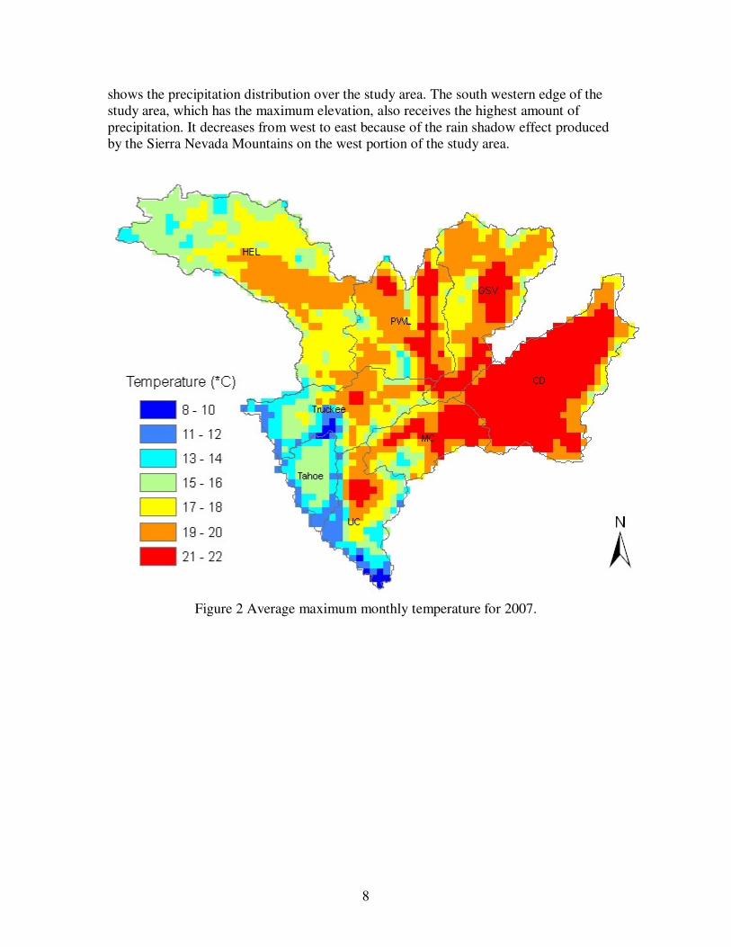
8

shows the precipitation distribution over the study area. The south western edge of the

study area, which has the maximum elevation, also receives the highest amount of

precipitation. It decreases from west to east because of the rain shadow effect produced

by the Sierra Nevada Mountains on the west portion of the study area.

Figure 2 Average maximum monthly temperature for 2007.

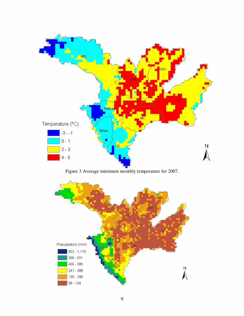
9

Figure 3 Average minimum monthly temperature for 2007.

10

Figure 4 Total precipitation for 2007.

Analysis of precipitation data for the eight sub regions shows that annual precipitation

has experienced an increasing trend in six of the sub regions excluding Honey Eagle

Lakes and Upper Carson (Table 2). Figure 5 shows the variation in annual precipitation

in the Lake Tahoe Basin. Breaking down the annual precipitation trends into the four

seasons reveal that the increase is not uniform throughout the year. All but GSV show a

decrease in winter precipitation with UC experiencing the largest rate of decrease. In case

of spring season, all regions at lower altitudes experienced an increasing trend in

precipitation during the study period and all the high altitude regions show a decline in

spring precipitation. However, for the summer months, all regions show similar

increasing trends. The high altitude regions which show a decreasing trend for spring

precipitation show the greatest rates of increase in fall precipitation thus more than

compensating for the decline experienced in winter and spring seasons. The lower

regions also experience an increase in fall precipitation but at a smaller rate.

y = 0.3163x + 169.43

R2 = 0.0021

400

600

800

1000

1200

1400

1600

1895 1905 1915 1925 1935 1945 1955 1965 1975 1985 1995 2005

Year

(mm

)

Precip 5 per. Mov. Avg. (Precip) Linear (Precip)

Figure 5 Annual precipitation for Lake Tahoe Basin.

Table 2 Annual average rate of change in precipitation. Precipitation Trends Winter Spring Summer Fall Annual

Carson Desert CD -0.0068 0.1335 0.1216 0.1006 0.3423

Granite Springs Valley GSV 0.0007 0.1594 0.1471 0.1192 0.4283

Honey Eagle Lakes HEL -0.0432 -0.0679 0.114 -0.0022 -0.0198

Middle Carson MC -0.1408 0.0157 0.114 0.1052 0.0756

Pyramid Winnemucca Lakes PWL -0.1414 0.0165 0.1051 0.0579 0.0343

Lake Tahoe Tahoe -0.0797 -0.2516 0.1663 0.5514 0.3163

Truckee River Truckee -0.0086 -0.2608 0.1221 0.4065 0.214

Upper Carson UC -0.3452 -0.2393 0.1526 0.3977 -0.0823

Entire Study Area Entire -0.0718 -0.0233 0.1255 0.1500 0.1607

The monthly maximum and minimum temperatures for the Lake Tahoe basin have been

rising as seen in Figure 6 and Figure 7. Temperature trends for all sub regions in the

study area show consistent rising trends over the period of study (Table 3 & Table 4).

11

The analyses of average monthly minimum and maximum temperatures show that the

rate of change was not uniform for the four seasons.

Maximum temperatures increased all over the study area for all seasons but average

maximum temperature for winters displayed the highest rate of increase. Minimum

temperatures on the other hand show a reversed trend for the winter season with the

lowest rate of increase of all seasons.

y = 0.0108x - 7.9244

R2 = 0.171

10

11

12

13

14

15

16

1895 1905 1915 1925 1935 1945 1955 1965 1975 1985 1995 2005

Year

(Cels

ius)

Tmax 5 per. Mov. Avg. (Tmax) Linear (Tmax)

Figure 6 Annual average monthly maximum temperatures for Lake Tahoe Basin.

y = 0.0157x - 32.129

R2 = 0.3785

-4

-3

-2

-1

0

1

1895 1905 1915 1925 1935 1945 1955 1965 1975 1985 1995 2005

Year

(Cels

ius)

Tmin 5 per. Mov. Avg. (Tmin) Linear (Tmin)

Figure 7 Annual average monthly minimum temperatures for Lake Tahoe Basin.

Table 3 Annual average rate of change in maximum temperatures. Maximum Temperature Winter Spring Summer Fall Annual

Carson Desert CD 0.0234 0.0121 0.0109 0.0107 0.0143

Granite Springs Valley GSV 0.017 0.0101 0.0102 0.0006 0.0095

12

Honey Eagle Lakes HEL 0.0202 0.0103 0.0091 0.0004 0.01

Middle Carson MC 0.015 0.0093 0.0108 0.0064 0.0104

Pyramid Winnemucca Lakes PWL 0.0214 0.0123 0.0139 0.0032 0.0127

Lake Tahoe Tahoe 0.0144 0.011 0.0101 0.0077 0.0108

Truckee River Truckee 0.0172 0.0122 0.0201 0.0088 0.0146

Upper Carson UC 0.0131 0.011 0.0088 0.009 0.0105

Entire Watershed Entire 0.0189 0.011 0.0115 0.005 0.0116

Table 4 Annual average rate of change in minimum temperatures. Minimum Temperature Winter Spring Summer Fall Annual

Carson Desert CD 0.0122 0.0142 0.0101 0.0093 0.0153

Granite Springs Valley GSV 0.0095 0.0072 0.0133 0.0098 0.001

Honey Eagle Lakes HEL 0.0064 0.0095 0.0164 0.0143 0.0117

Middle Carson MC 0.012 0.0155 0.0171 0.0179 0.0155

Pyramid Winnemucca Lakes PWL 0.0101 0.0119 0.0198 0.0166 0.0147

Lake Tahoe Tahoe 0.0145 0.0144 0.017 0.0169 0.0157

Truckee River Truckee 0.0067 0.01 0.0122 0.0136 0.011

Upper Carson UC 0.0118 0.0116 0.0214 0.0167 0.0154

Entire Watershed Entire 0.0096 0.0104 0.0153 0.0146 0.0125

2.2 VIC Hydrological Model This study also uses the outputs of the Variable Infiltration Capacity (VIC) hydrological

model to analyze the changes occurring to the snow water equivalent (SWE) in the region

between 1915 and 2005. Daily gridded meteorological data obtained from the Surface

Water Modeling group at the University of Washington from their web site at

http://www.hydro.washington.edu/Lettenmaier/Data/gridded/, the development of which

is described by Hamlet and Lettenmaier (2005) and Maurer et al., (2002). VIC is a

macroscale hydrologic model that balances both surface energy and water over a grid

mesh, typically at resolutions ranging from a fraction of a degree to several degrees

latitude by longitude. The primary sources of meteorological data used in the data-

processing sequence include NCDC Co-op data, monthly time step HCN and HCCD data,

and PRISM data (Hamlet and Lettenmaier, 2005).

Most of the grid cells selected for the analysis lie along the periphery of Lake Tahoe.

Figure 8 displays the grid cells from VIC model outputs which are used for the analysis

of SWE changes. Each grid cell covers 1/8th of a degree grid cell (i.e. 13.8 km along the

longitudes and approximately 10.1 km along the latitudes). To determine the changes in

SWE over the time horizon afforded by VIC data, average SWE for January was

calculated for each year. Figure 9 shows that the mean SWE for January has increased by

almost 1mm per year. SWE calculations for April 1 were also carried out which showed a

decline for all the grid cells. Therefore, to understand this inconsistency, March 1 and

February 1 SWE were calculated for all the cells. The results show a rise in the SWE for

January 1 and February 1 for all the grid cells whereas all the grid cells evaluated display

a decline in April 1 SWE (Table 5). The average change in SWE per year ranges from

0.22 mm/yr to 1.07 mm/yr.

13

Figure 8 Location of VIC grid cells used for estimating SWE variations.

14

y = 0.9498x - 1586.7

R2 = 0.0227

0

100

200

300

400

500

600

700

1915 1925 1935 1945 1955 1965 1975 1985 1995 2005Year

(SW

E m

m)

SWE Linear (SWE) 5 per. Mov. Avg. (SWE)

Figure 9 Mean January SWE variation for grid cell #1.

y = -0.6052x + 1697.4

R2 = 0.0033

0

200

400

600

800

1000

1200

1400

1915 1925 1935 1945 1955 1965 1975 1985 1995 2005Year

(SW

E m

m)

SWE Linear (SWE) 5 per. Mov. Avg. (SWE)

Figure 10 April 1 SWE for grid cell #2.

Table 5 VIC results for SWE variations.

Average Change/Year (mm)

Grid

Cell Latitude Longitude Mean Jan 1-Apr 1-Mar 1-Feb 1-Jan

1 38.6875 -119.938 1.079 -0.0413 0.3831 0.9179 1.1618

2 38.6875 -120.063 0.9498 -0.6052 0.0154 0.7107 1.1386

3 38.8125 -119.813 0.2191 -0.1405 -0.1725 0.0609 0.3279

4 38.8125 -119.938 1.0508 -0.0709 0.2505 0.8597 1.1997

5 38.8125 -120.063 1.0261 -0.3269 0.2751 0.8396 1.1811

6 38.8125 -120.188 0.4951 -0.5896 -0.2314 0.2683 0.7333

7 38.9375 -119.938 0.5468 -0.3521 -0.1536 0.363 0.7069

8 38.9375 -120.188 1.0262 -0.5268 0.1914 0.8565 1.1877

9 39.0625 -120.188 0.4471 -1.072 -0.4237 0.22 0.6665

10 39.1875 -120.188 0.7225 -0.101 0.1599 0.5842 0.8456

11 39.3125 -120.438 0.9876 -0.4272 0.1807 0.6736 1.1597

12 39.0625 -119.938 0.2212 -0.4176 -0.1687 0.0821 0.4019

13 39.1875 -119.938 0.3266 -0.5255 -0.2924 0.1996 0.5101

15

3 FUTURE CLIMATE CHANGE

3.1 Emission Scenarios Green House Gas (GHG) emissions are dependent on a large number of factors which are

interrelated in very complex and dynamic system. The emissions are driven by factors

such as demographic development, socio-economic development, and technological

change. Predicting the evolution of these factors is extremely difficult but a number of

possible alternative paths, along which the future might unfold, can be postulated. These

scenarios assist in analyzing the effects of changing climate on available resources and

comparing available measures to mitigate its effects. Emission scenarios provide us with

several alternative paths along which the world may progress and thus how GHG

emissions might change over time. A number of such scenarios based on a wide array of

driving forces have been developed by researchers all around the world.

Four different narrative storylines describing a range of possible alternative paths,

excluding “surprise” or “disaster” scenarios have been generated by the IPCC based on

literature. These were developed to describe consistently the relationships between

emission driving forces and their evolution and add context for the scenario

quantification. Each storyline represents different combination of demographic, social,

economic, technological, and environmental developments. All scenarios based on the

same storyline constitute a scenario “family”. Each scenario represents a specific

quantitative interpretation of one of four storylines described below.

Four qualitative storylines yield four sets of scenarios called “families”: A1, A2, B1, and

B2. All are equally valid with no assigned probabilities of occurrence. The set of

scenarios consists of six scenario groups drawn from the four families described in Table

6: one group each in A2, B1, B2, and three groups within the A1 family, characterizing

alternative developments of energy technologies: A1FI (fossil fuel intensive), A1B

(balanced), and A1T (predominantly non-fossil fuel). Within each family and group of

scenarios, some share “harmonized” assumptions on global population, gross world

product, and final energy. These are marked as “HS” for harmonized scenarios. “OS”

denotes scenarios that explore uncertainties in driving forces beyond those of the

harmonized scenarios.

The A1 storyline and scenario family describes a future world of very rapid economic

growth, global population that peaks in mid-century and declines thereafter, and the rapid

introduction of new and more efficient technologies. Major underlying themes are

convergence among regions, capacity building, and increased cultural and social

interactions, with a substantial reduction in regional differences in per capita income. The

A1 scenario family develops into three groups that describe alternative directions of

technological change in the energy system. The three A1 groups are distinguished by

their technological emphasis: fossil intensive (A1FI), non-fossil energy sources (A1T), or

a balance across all sources (A1B).

The A2 storyline and scenario family describes a very heterogeneous world. The

underlying theme is self-reliance and preservation of local identities. Fertility patterns

16

across regions converge very slowly, which results in continuously increasing global

population. Economic development is primarily regionally oriented and per capita

economic growth and technological changes are more fragmented and slower than in

other storylines.

The B1 storyline and scenario family describes a convergent world with the same global

population that peaks in mid-century and declines thereafter, as in the A1 storyline, but

with rapid changes in economic structures toward a service and information economy,

with reductions in material intensity, and the introduction of clean and resource-efficient

technologies. The emphasis is on global solutions to economic, social, and environmental

sustainability, including improved equity, but without additional climate initiatives.

The B2 storyline and scenario family describes a world in which the emphasis is on local

solutions to economic, social, and environmental sustainability. It is a world with

continuously increasing global population at a rate lower than A2, intermediate levels of

economic development, and less rapid and more diverse technological change than in the

B1 and A1 storylines. While the scenario is also oriented toward environmental

protection and social equity, it focuses on local and regional levels.

Table 6 Summary of four SRES storylines

A1 A2

World Market Oriented Differentiated

Economy Fastest Per Capita

Regionally oriented, lowest per capita growth

Population 2050 peak, then decline Continuously increasing

Governance Strong regional

Self reliance with preservation of local

identities

Technology

Three groups: A1F1 (Fossil fuel), A1T

(Non-fossil), & A1B Balanced)

Slowest and the most fragmented

growth

B1 B2

World Convergent Local solutions

Economy

Service and information based, lower

growth than A1 Intermediate growth

Population Same as A1

Continuously increasing at a rate lower

than A2

Governance

Global solutions to economic, social

and environmental sustainability

Regional solutions to environmental

protection and social equity

Technology Clean and resource efficient

More rapid than A2; less rapid and

more diverse than A1/B1

The shortwave impact of changes in boundary-layer clouds, and to a lesser extent

midlevel clouds, constitutes the largest contributor to inter-model differences in global

cloud feedbacks.

17

3.2 Climate Models Eighteen modeling groups performed a set of coordinated, standard experiments, and the

resulting model output, analyzed by hundreds of researchers worldwide, forms the basis

for much of the current IPCC assessment of model results. A total of 23 models by 18

groups are currently used by IPCC to generate the future climate change scenarios.

(Randall et al., 2007). The modeling groups and models used for this purpose are

mentioned in Table 7.

Table 7 AOGCMs featured in IPCC Reports.

Model Sponsors/Country References

CSIRO-MK3 Commonwealth Scientific and Industrial Research Organisation

(CSIRO) Atmospheric Research, Australia

Gordon et al., 2002; O’Farrell,

1998.

MIROC3.2

(medres)

Center for Climate System Research (University of Tokyo),

National Institute for Environmental Studies , and Frontier

Research Center for Global Change (JAMSTEC), Japan

K-1 Developers, 2004;

Oki and Sud, 1998.

UKMO-

HadCM3

Hadley Centre for Climate Prediction and Research/Met Office,

UK

Pope et al., 2000;

Gordon et al., 2000;

Cattle and Crossley,1995; Cox et

al., 1999.

Figure 11 shows the continuation of the 20th-century simulations for warming trends.

Lines show the multi-model means, shading denotes the ±1 standard deviation range of

individual model annual means. Discontinuities between different periods have no

physical meaning and are caused by the fact that the number of models that have run a

given scenario is different for each period and scenario, as indicated by the coloured

numbers given for each period and scenario at the bottom of the panel. For the same

reason, uncertainty across scenarios should not be interpreted from this figure (see

Section 10.5.4.6 for uncertainty estimates).

18

Figure 11: Multi-model means of surface warming (relative to 1980–1999) for the

scenarios A2, A1B and B1. (Source: IPCC FAR)

3.3 Climate Change Projections Accurate climate projections play a crucial role in determining the success of water

management plans by providing an estimate of changes occurring to temperature and

precipitation patterns which govern water availability. This section of the report compiles

the climate change projections up to the end century obtained from three major coupled

atmosphere-ocean general circulation models MIROC-M3, UKMO-HadCM3, and

CSIRO-Mk3.0 for three emission scenarios namely A2, A1B, and B1.

Figure 12 shows the time series of globally averaged (left) surface warming (surface air

temperature change, °C) and (right) precipitation change (%) from the various global

coupled models for the scenarios A2 (top), A1B (middle) and B1 (bottom). Numbers in

parentheses following the scenario name represent the number of simulations shown.

Values are annual means, relative to the 1980 to 1999 average from the corresponding

20th-century simulations, with any linear trends in the corresponding control run

simulations removed. A three-point smoothing was applied. Multi-model (ensemble)

mean series are marked with black dots.

19

Figure 12: Time series of globally averaged surface air temperature and precipitation

changes. (Source: IPCC FAR)

Confidence in climate models comes from the physical science behind their creation, and

their skill at reproducing observed climate and past climate changes. Models have proven

to be extremely important tools for simulating and understanding climate, and there is

considerable confidence that they are able to provide credible quantitative estimates of

future climate change, particularly at larger scales. Nonetheless, most models still suffer

from a number of drawbacks which impose significant limitations on their results. Some

of these drawbacks include their ability in representing clouds and man made aerosols etc

which lead to uncertainties in the magnitude, timing, and spatial detail of predicted

climate change. Nevertheless, over several decades of model development, they have

consistently provided a robust and unambiguous picture of significant climate warming in

response to increasing greenhouse gases at a global scale. However, since confidence in

the changes projected by global models decreases at smaller scales, other techniques,

such as the use of regional climate models, or downscaling methods, should be preferred

for the study of regional and local scale climate change.

20

Figure 13 Precipitation change by mid 21

st century as suggested by ensemble results from

the three model outputs used in this study.

Figure 13 shows the anticipated mean precipitation departure by mid 21st century. The

figure shows the estimated change in annual precipitation averaged over a period between

2040 and 2060. The change is compared to the mean historic data from 1961 to 1990.

Figure 14 shows the reduction in precipitation by the end of 21st century. Both figures

show significant decreases in annual precipitation in the high altitude regions of the study

area. This region corresponds to the watershed of Lake Tahoe, Truckee River, and the

Carson River and hence a decrease in precipitation in this area can significantly reduce

the flow into these water bodies.

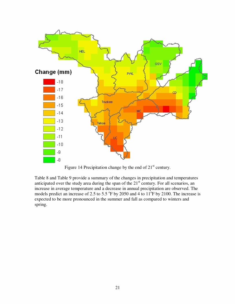
21

Figure 14 Precipitation change by the end of 21

st century.

Table 8 and Table 9 provide a summary of the changes in precipitation and temperatures

anticipated over the study area during the span of the 21st century. For all scenarios, an

increase in average temperature and a decrease in annual precipitation are observed. The

models predict an increase of 2.5 to 5.5 oF by 2050 and 4 to 11

oF by 2100. The increase is

expected to be more pronounced in the summer and fall as compared to winters and

spring.

22

Table 8 (a-c) Ensemble average from MIROC-M3, UKMO-HadCM3, and CSIRO-Mk3.0

models Summary of anticipated changes in precipitation and temperature by mid 21st

century under emission scenarios (a) A2, (b) A1B, and (c) B1.

Table 8(b)

Period Variable Change Units

Dec-Feb Temp 4.50 F

Mar-May 3.50 F

Jun-Aug 5.50 F

Sep-Nov 5.50 F

Annual 5.50 F

Dec-Feb Precip -6.00 %

Mar-May -15.00 %

Jun-Aug -21.84 %

Sep-Nov -14.92 %

Annual -7.50 %

Table 8(a)

Period Variable Change Units

Dec-Feb Temp 4.00 F

Mar-May 4.50 F

Jun-Aug 5.00 F

Sep-Nov 5.00 F

Annual 5.50 F

Dec-Feb Precip 7.50 %

Mar-May -18.50 %

Jun-Aug -15.91 %

Sep-Nov -7.00 %

Annual -11.00 %

Table 8(c)

Period Variable Change Units

Dec-Feb Temp 3.50 F

Mar-May 2.50 F

Jun-Aug 4.50 F

Sep-Nov 4.00 F

Annual 4.00 F

Dec-Feb Precip -3.00 %

Mar-May -7.00 %

Jun-Aug -6.00 %

Sep-Nov 1.50 %

Annual -4.50 %

23

Table 9 (a-c) Ensemble average from MIROC-M3, UKMO-HadCM3, and CSIRO-Mk3.0

models Summary of anticipated changes in precipitation and temperature by the end of

21st century under emission scenarios (a) A2, (b) A1B, and (c) B1.

Table 9 (a)

Period Variable Change Units

Dec-Feb Temp 6.50 F

Mar-May 6.50 F

Jun-Aug 11.00 F

Sep-Nov 8.50 F

Annual 8.50 F

Dec-Feb Precip -4.50 %

Mar-May -29.33 %

Jun-Aug -9.44 %

Sep-Nov 9.50 %

Annual -7.00 %

Table 9(b)

Period Variable Change Units

Dec-Feb Temp 6.50 F

Mar-May 5.50 F

Jun-Aug 9.50 F

Sep-Nov 7.50 F

Annual 7.50 F

Dec-Feb Precip -11.00 %

Mar-May -17.00 %

Jun-Aug -16.50 %

Sep-Nov -8.18 %

Annual -13.00 %

Table 9(c)

Period Variable Change Units

Dec-Feb Temp 4.50 F

Mar-May 4.00 F

Jun-Aug 6.50 F

Sep-Nov 5.50 F

Annual 6.00 F

Dec-Feb Precip -12.50 %

Mar-May -17.00 %

Jun-Aug -17.00 %

Sep-Nov -1.17 %

Annual -10.50 %

24

4 CONCLUSIONS

Analysis of precipitation data shows that annual precipitation has increased during the

last century. On dividing the trends into the four seasons, it was observed that the

increase was not consistent for all the seasons. Winter precipitation has decreased over

the last century whereas summer and fall precipitation has increased. Furthermore, the

largest decrease in winter precipitation was experienced by the regions located at a high

altitude in the Sierra Nevada Mountains. These regions are responsible for feeding Lake

Tahoe, the Truckee River and the Carson River. Therefore, a decrease in winter

precipitation in these regions means lesser snowpack and consequently lower inflows into

the water bodies.

The results from VIC outputs show a rise in the SWE for January 1 and February 1 for all

the grid cells whereas all the grid cells evaluated display a decline in April 1 SWE. These

results obtained from VIC outputs are in agreement with the findings from PRISM data

which suggest that precipitation during the fall season (Oct to Dec) has increased during

the same period. The lowered SWE in the later half of winter months also corroborates

the finding from PRISM data which shows that precipitation during the winter months

has decreased.

Temperature trends for all sub regions in the study area show consistent rising trends over

the last century. Increased temperatures in combination with changing precipitation

patterns can change the hydrology of the study area. The results from this study cannot

conclusively estimate the individual effects of temperature and precipitation changes on

SWE but this combination is likely to be a major factor causing the shifting of SWE bulk

towards the first half of the winters.

Future estimates from the climate models used in this study show decreases in annual

precipitation throughout the study area. In addition the projections suggest a decrease in

precipitation for all seasons throughout the watershed for all emission scenarios. The

decreases are greater in magnitude in the high altitude regions of the study area. This

region corresponds to the watershed of Lake Tahoe, the Truckee River, and the Carson

River and hence a decrease in precipitation in this area can significantly reduce the flow

into these water bodies. This finding however is inconsistent with the results obtained

from PRISM and VIC outputs which show an increase in summer and fall precipitation in

the study area over the last century. This inconsistency could be a result of the

topography of the study area and the inability of climate models to generate accurate

future trends for relatively small regions with abrupt changes in topography.

(notes: I have a general concern about the significance of the trend lines created in the

Excel charts. The very low R2 points one to conclude that the trend might not be

statistically significant. If possible have Dinesh add 95% confidence interval to some of

key statistics. I am going to try to do some time series test on some of the data to see if

the trend lines are significant.

25

5 REFERENCES

Cattle, H., and J. Crossley (1995) Modelling Arctic climate change. Philos. Trans. R. Soc.

London Ser. A, 352, 201–213.

Cayan, D. R., S. A. Kammerdiener, M. D. Dettinger, J. M. Caprio, and D. H. Peterson,

(2001) Changes in the onset of spring in the western United States. Bull. Am. Meteor.

Soc., 82, 399–415.

Cayan, D. R., E. P. Maurer, M. D. Dettinger, M. Tyree and K. Hayhoe (2008) Climate

Change Scenarios for the California Region. Clim. Change 87, 21-42.

Christensen, N. S., A. W. Wood, D. P. Lettenmaier, and R. N. Palmer (2004) Effects of

Climate Change on the Hydrology and Water Resources of the Colorado River Basin.

Clim. Change 62, 337–363.

Cox, P.M., et al., (1999) The impact of new land surface physics on the GCM

simulation of climate and climate sensitivity. Clim. Dyn., 15, 183–203.

Daly, C., R.P. Neilson, and D.L. Phillips (1994) A Statistical-Topographic Model for

Mapping Climatological Precipitation over Mountanious Terrain. J. Appl. Meteor., 33,

140-158.

Daly C, G. H. Taylor, W. P. Gibson, T. W. Parzybok, G. L. Johnson, P. Pasteris (2001)

High-quality spatial climate data sets for the United States and beyond. Trans. Am. Soc.

Agric. Eng. 43:1957–1962

Daly, C., W. P. Gibson, G. H. Taylor, G. L. Johnson, P. Pasteris.(2002) A knowledge-

based approach to the statistical mapping of climate. Clim. Res., 22, 99-113.

Dettinger, M. D. (2005) From Climate Change Spaghetti to climate change distributions

for 21st Century, San Francisco Estuary and Watershed Science, 3(1).

Dettinger, M. D., and D. R. Cayan (1995) Large-scale atmospheric forcing of recent

trends toward early snowmelt runoff in California. J. Clim., 8, 606–623.

Giorgi, F. and L. O. Mearns (1991) Approaches to the simulation of regional climate

change: A review. Reviews in Geophysics, 29, 191-216.

Giorgi, F., C. S. Brodeur, and G. T. Bates (1994) Regional climate change scenarios over

the United States produced with a nested regional climate model: Spatial and seasonal

characteristics. J. Clim. 7, 375–399.

26

Gordon, C., et al., (2000): The simulation of SST, sea ice extents and ocean heat

transports in a version of the Hadley Centre coupled model without flux adjustments.

Clim. Dyn. 16, 147–168.

Gordon, H.B., et al., (2002) The CSIRO Mk3 Climate System Model. CSIRO

Atmospheric Research Technical Paper No. 60, Commonwealth Scientific and Industrial

Research Organisation Atmospheric Research, Aspendale, Victoria, Australia, 130 pp,

http://www.cmar.csiro.au/e-print/open/gordon_2002a.pdf.

Groisman, P. Y., R. W. Knight, T. R. Karl, D. R. Easterling, B. Sun and J. H. Lawrimore

(2004) Contemporary changes of the hydrological cycle over the contiguous United

States: trends derived from in situ observations. J. Hydrometeorol., 5, 64-85.

Hamlet A. F., D. P. Lettenmaier (2005) Production of Temporally Consistent Gridded

Precipitation and Temperature Fields for the Continental U.S. J of Hydrometeorol. 6 (3),

330-336.

Hamlet, A. F. and D. P. Lettenmaier (1999) Effects of Climate Change on Hydrology and

Water Resources in the Columbia River Basin. J. of Am. Water Res Assn 35(6), 1597–

1623.

Hengeveld, H., B. Whitewood and A. Fergusson (2005) An Introduction to Climate

Change: A Canadian Perspective. Environment Canada, Downsview, Ontario, 55 pp.

IPCC, 2007: Climate Change 2007: The Physical Science Basis. Contribution of Working

Group I to the Fourth Assessment Report of the Intergovernmental Panel on Climate

Change. Cambridge University Press, Cambridge, United Kingdom and New York, NY,

USA.

Karl, T. R., P. Y. Groisman, R. W. Knight, and R. R. Heim (1993) Recent variations of

snow cover and snowfall in North America and their relations to precipitation and

temperature variations. J. of Clim. 6, 1327–1344.

Kim, J. (2005) A projection of the effects of the climate change induced by increased

CO2 on extreme hydrologic events in the western U.S., Clim. Change.

Knowles, N., M. D. Dettinger, and D. R. Cayan (2006) Trends in snowfall versus rainfall

in the Western United States, J. Clim. 19, 4545– 4559.

Labat, D., Y. Godderis, J.L. Probst, J.L. Guyot, (2004) Evidence for global runoff

increase related to climate warming. Adv. in Water Res. 27, 631–642.

K-1 Model Developers, (2004): K-1 Coupled Model (MIROC) Description. K-1

Technical Report 1 [Hasumi, H., and S. Emori (eds.)]. Center for Climate System

Research, University of Tokyo, Tokyo, Japan, 34 pp.

http://www.ccsr.u-tokyo.ac.jp/kyosei/hasumi/MIROC/tech-repo.pdf.

27

Kunkel, K. E. (2003)Temporal variations of extreme precipitation events in the United

States: 1895-2000. Geophys. Res. Lett., 30.

Lemke, P., et al. (2007) Observations: Changes in snow, ice and frozen ground, in

Climate Change 2007: The Physical Science Basis. edited by S. Solomon et al., pp. 337–

383, Cambridge Univ. Press, New York.

Lettenmaier, D. P., E. F. Wood, and J. R. Wallis (1994) Hydroclimatological trends in

the continental United States, 1948–88. J. Clim, 7, 586–607.

Leung, L. R., Y. Qian, and X. Bian (2003) Hydroclimate of the western United States

based on observations and regional climate simulation of 1981– 2000, part I: Seasonal

statistics, J. Clim., 16(12), 1892– 1911.

Maurer, E. P., A. W. Wood, J. C. Adam, D. P. Lettenmaier, and B. Nijssen (2002) A

Long-Term Hydrologically Based Dataset of Land Surface Fluxes and States for the

Conterminous United States. J. of Clim. 15, 3237-3251.

Maurer, E. P. (2007) Uncertainty in hydrologic impacts of climate change in the Sierra

Nevada, California under two emissions scenarios. Clim. Change, 82, 309–325.

Maurer, E. P. and P. B. Duffy (2005) Uncertainty in projections of streamflow changes

due to climate change in California. Geophys. Res. Lett., 32.

Mearns, L., F. Giorgi, L. McDaniel, and C. Shields (1995a) Analysis of daily variability

of precipitation in a nested regional climate model: Comparison with observation and

doubled CO2 results. Global Planet. Change 10, 55–78.

Mearns, L., F. Giorgi, L. McDaniel, and C. Shields (1995b) Analysis of variability and

diurnal range of daily temperature in nested regional climate model: Comparison with

observation and doubled CO2 results. Clim. Dyn. 10, 55–78.

Millar, C. I., W. B. Woolfenden (1999) The Role of Climate Change in Interpreting

Historical Variability. Ecological Applications 9(4), 1207-1216.

Mote, P. W. (2003) Trends in snow water equivalent in the Pacific Northwest and their

climatic causes. Geophys. Res. Lett., 30, 1601, doi: 10.1029/2003GL017258.

Mote, P. W., A. F. Hamlet, M. P. Clark, and D. P. Lettenmaier (2005) Declining

mountain snowpack in western North America. Bull. Amer. Meteor. Soc., 86, 39–49.

Nanus, L., D. H. Campbell, G. P. Ingersoll, D. W. Clow, and M. A. Mast, (2003)

Atmospheric deposition maps for the Rocky Mountains. Atm. Env. 37, 4881–4892.

28

O’Farrell, S.P. (1998) Investigation of the dynamic sea ice component of a coupled

atmosphere sea-ice general circulation model. J. Geophys. Res.,103, 15751–15782.

Oki, T., and Y. C. Sud (1998): Design of total runoff integrating pathways (TRIP)—A

global river channel network. Earth Interactions 2, 1–37.

Payne, J. T., A. W. Wood, A. F. Hamlet, R. N. Palmer and D. P. Lettenmaier (2004).

Mitigating the effects of climate change on the water resources of the Columbia River

basin. Clim. Change 62, 233-256.

Pierce, D. W., T. P. Barnett, H. G. Hidalgo, T. Das, C. Bonfils, B. D. Santer, G. Bala, M.

D. Dettinger, D. R. Cayan, A. Mirin, A. W. Wood and T. Nozawa (2008) Attribution of

Declining Western U.S. Snowpack to Human Effects. J. Climate, 21, 6425-6444.

Pope, V.D., M.L. Gallani, P.R. Rowntree, and R.A. Stratton (2000) The impact of new

physical parametrizations in the Hadley Centre climate model: HadAM3. Clim. Dyn., 16,

123–146.

Pupacko, A. (1993) Variations in northern Sierra Nevada streamflow: Implications of

climate change. Water Resour. Bull. 29(2), 283-290.

Randall, D. A., R. A. Wood, S. Bony, R. Colman, T. Fichefet, J. Fyfe, V. Kattsov, A.

Pitman, J. Shukla, J. Srinivasan, R. J. Stouffer, A. Sumi and K. E. Taylor (2007) Cilmate

Models and Their Evaluation. In: Climate Change 2007: The Physical Science Basis.

Contribution of Working Group I to the Fourth Assessment Report of the

Intergovernmental Panel on Climate Change [Solomon, S., D. Qin, M. Manning, Z. Chen,

M. Marquis, K.B. Averyt, M.Tignor and H.L. Miller (eds.)]. Cambridge University Press,

Cambridge, United Kingdom and New York, NY, USA.

Regonda, S. K., B. Rajagopalan, M. Clark, and J. Pitlick (2005) Seasonal cycle shifts in

hydroclimatology over the western United States. J. Climate 18, 372–384.

Rood, S. B., G. M. Samuelson, J. K.Weber and K. A.Wywrot (2005) Twentieth-century

decline in streamflows fromthe hydrographic apex of NorthAmerica. J. Hydrol. 306, 215-

233

Shein, K. A. (2006) State of the climate in 2005, including executive summary. Bull.

Amer. Meteorol. Soc., 87, 801-805,

Stewart, I. T., Cayan, D. R., Dettinger, M. D. (2004) Changes in snowmelt runoff timing

in western North America under a 'business as usual' climate change scenario. Clim.

Change, 62, 217-232.

Stewart, I.T., Cayan D. R., Dettinger, M. D. (2005) Changes toward Earlier Streamflow

Timing across Western North America. J. Clim., 18(8), 1136–1155.

29

Seager R., Ting M., Held I., Kushnir Y., Lu J., Vecchi G., Huang H. P., Harnik N., Lau N.

C., Li C. et al. (2007) Model projections on an inminent transition to a more arid climate

in southwestern North America. Science 316: 1181– 1184.

Trenberth, K. E., A. Dai, R. M. Rasmussen, and D. B. Parsons (2003) The changing

character of precipitation. Bull. Amer. Meteor. Soc., 84, 1205–1217.

Trenberth, K. E., L. Smith, T. Qian, A. Dai, and J. Fasullo (2007), Estimates of the global

water budget and its annual cycle using observational and model data, J. Hydrometeorol.

8, 758-769.

US Census Bureau, Population Division. http://www.census.gov/popest/cities/SUB-

EST2008-states.html Retrieved on July 18, 2009.

VanRheenen, N. T., A. W. Wood, R. N. Palmer and D. P. Lettenmaier (2004) Potential

Implications of PCM Climate Change Scenarios for California Hydrology and Water

Resources. Clim. Change 62, 257–281.

Vicuna S., E. P. Maurer, B. Joyce, J. A. Dracup, D. Purkey (2007) The sensitivity of

California water resources to climate change scenarios. J Am Water Res Assoc 43(2):

482 –498

Vincent, L. A., X. Zhang, and W. D. Hogg (1999) Maximum and minimum temperature

trends in Canada for 1895–1995 and 1945–1995. 10th Symp. on Global Change Studies,

Dallas, TX, Amer. Meteor. Soc., 95–98.

Walter, M. T., D. S. Wilks, J.-Y. Parlange, and R. L. Schneider (2004) Increasing

evapotranspiration from the conterminous United States, J. Hydrometeorol., 5, 405– 408.

30

6 APPENDICES

6.1 Processing steps for PRISM Dataset

Step 1.Downloading Data: PRISM data can either be downloaded interactively from

(http://mole.nacse.org/prism/nn/index.phtml?vartype=ppt&year0=2003&year1=2

003) or from the PRISM Group’s ftp site

(ftp://prism.oregonstate.edu/pub/prism/us/grids/)

Step 2.Unzipping: The files downloaded from the sources mentioned in Step 1 were

unzipped and converted to ascii files by changing the extension to <*.asc>. Due to

a large number of files, individual unzipping would have been impractical.

Therefore, “7-zip” freeware was used for this process.

Step 3.Processing in ArcGIS: Resulting files from Step 2 were imported into ArcGIS and

converted into raster format. “Modelbuilder” feature in ArcMap was used to

automate the processing of files for this step and all other subsequent steps due to

the large number of files.

Step 4.Raster files obtained from Step 3 were then clipped using the watershed shapefiles.

Step 5.Attributes tables were created for all the clipped raster files.

Step 6.Additional field (“precip” for precipitation files and “temp” for temperature files)

was created in the attributes tables for the clipped raster files to hold the product

of the fields “Value” and “Count”.

Step 7.“Summary Statistics” tool in ArcMap was used to obtain the mean of the field

“precip/temp” and sum of the field “count”. In addition,

Step 8.Summary statistics obtained as *.dbf files, for each corresponding raster file, were

converted into *.xls files for processing in Matlab.

Step 9.A Matlab program was used to read the statistics of “precip/temp” and “Count”

from the .xls files created in Step 8.

Step 10.The average temperature or depth of precipitation over the watershed were

calculated using

PC /×Υ=Χ

Where

X =

Y = precip or temp read in Step 9

C = Count read in Step 9

P = Number of pixels the raster file for the corresponding watershed.

31

6.2 Notes: ArcMap was unable to process all the files simultaneously using Modelbuilder. Therefore,

files were processed one watershed at a time.

Due to naming protocols in ArcMap, files obtained after processing had complicated

names. Renaming was found to be useful to prevent mixing up of files.

Theoretically it is possible to combine Steps 3 to 8 in one model but difficulties were

encountered while running these processes in a single model. Modelbuilder failed to

execute certain steps when multiple processes were combined in a single model.

The following Matlab code was used to execute the process described in Step 9.

xlsFiles = dir(‘Path\*.xls')

Matrix = zeros (length(xlsFiles),1)

for k = 1:length(xlsFiles);

filename = xlsFiles(k).name

data = xlsread(filename, 'a2:a2')

Matrix(k) = data

end

xlswrite ('Path’\output_filename.xls', Matrix, 'Sheet1')