aer appendix political resource curse
TRANSCRIPT

The Political Resource Curse∗
Online Appendix
Fernanda Brollo
(University of Alicante)
Tommaso Nannicini
(Bocconi University, IGIER & IZA)
Roberto Perotti
(Bocconi University, IGIER, CEPR & NBER)
Guido Tabellini
(Bocconi University, IGIER, CEPR & CIFAR)
First version: September 2009
This version: June 2012
Abstract
This Appendix provides additional materials that are also discussed in the paper. In particu-
lar, Section A1 presents the theoretical derivations of some of the model’s results. Section A2
presents validity tests on the lack of manipulative sorting in the IBGE population estimates,
that is, the running variable of the fuzzy RD design implemented in the paper. Section A3
reports examples of violation episodes from the audit reports, in order to illustrate the cod-
ing of our measures of political corruption. Section A4 provides further robustness checks,
in order to show that the baseline estimation results are not sensitive to the definition of the
outcome variables, to functional form assumptions, or to sample restrictions.
JEL codes: D72, D73, H40, H77.
Keywords: government spending, corruption, political selection.
∗We gratefully acknowledge financial support by the European Research Council under grant No. 230088 and by Bocconi
University (Nannicini, Perotti, and Tabellini), by the Spanish Ministry of Education and Feder Funds under project SEJ
2007-62656 and by University of Alicante (Brollo). We thank Frederico Finan, Macartan Humphreys, Guy Michaels, and
seminar participants at AEA-ASSA Conference 2011, ASSET Conference 2010, Bologna University, CIFAR Meeting 2010,
Econometric Society World Conference 2010, EUI, FGV-SP, IEB-Barcelona, IGIER-Bocconi, INSPER, LACEA Conference
2010, LSE, MILLS, NBER Political Economy Program Meeting 2009, Oxford University, and Wallis Conference 2009 for
extremely helpful comments and suggestions; Eliana La Ferrara, Alberto Chong, and Suzanne Duryea for sharing their
data on the 1980 Census; Gaia Penteriani, Denise Cassia Badu Alencar, and Vitor Ugo de Oliveira for excellent research
assistance. E-mails: [email protected]; [email protected]; [email protected];

A1 Theoretical derivations
Equilibrium rents, holding constant the quality composition of the opponents
To solve the model, we work backwards. In the last period, whoever is in office sets max-
imal rents. This follows from the assumption that the expected penalty is insufficient to deter
corruption (αJ > 0 for all J). Hence, r2 = r ≡ ψτ irrespective of who is elected.
Next, consider the voters’ behavior in period 1. Since the period 2 policy is the same
irrespective of who is in office, voters only care about competence, and they vote for the candidate
with the higher expected competence. Thus, an incumbent of type J wins against an opponent
of type O if:
E(θ|g1, J) ≥ 1 + σO J, O = H,L (A1)
where the left hand side of (A1) is the expected value of θ conditional on the voters observation of
g1 and their knowledge of the incumbent’s type J, while the right hand side is the unconditional
mean of θ for an opponent of type O.
By equation (1) in the paper, it is easy to see that (see also Persson and Tabellini, 2000):
E(θ|g1, J) =g1
(τ − reJ1 )
(A2)
where reJ1 denotes the voter’s expectation of how an incumbent of type J sets rents in period 1.
Exploiting (1) once more we also have that, from the point of view of the incumbent
E(θ|g1, J) = θτ − rJ
1
τ − reJ1
(A3)
where rJ1 denotes the rents actually set by a type J incumbent. Thus, by (A1)-(A3), an in-
cumbent of type J running against an opponent of type O wins the election with a perceived
probability
pJO = Pr[θ ≥τ − reJ
1
τ − rJ1
(1 + σO)] (A4)
=1
2+ ξ(1 + σJ) − ξ
τ − reJ1
τ − rJ1
(1 + σO) (A5)
where the first equation follows from (A1)-(A3), and the second equation from the assumption
about the distribution of θ.1 More precisely, the above expression refers to the probability of
1Specifically, given that θ is drawn from a uniform distribution with density ξ and mean 1 + σJ ,
Pr[θ > X ] =1
2+ ξ(1 + σ
J− X)
1

being reappointed, as perceived by the incumbent when setting rents, conditional on knowing
the identity of the opponent.
When the incumbent sets policy, however, he does not yet know the identity of his future
opponent, and he assigns probabilities π and 1 − π to the events that the opponent will be of
type L and H , respectively. Thus, as perceived by the incumbent when choosing rents, the
relevant probability of reelection is:
pJ =1
2+ ξ(1 + σJ) − ξ
τ − reJ1
τ − rJ1
(1 + σ) (A6)
where σ is the expected competence of the opponent, as perceived by the incumbent when
setting rents in period 1:
1 + σ ≡ 1 + σ(1− 2π) (A7)
We are now ready to discuss the determination of public policy in period 1. The incumbent
maximizes equation (3) in the paper with respect to r1, subject to (A6) and, by the incentive
compatibility condition, taking the voters expectations reJ1 as given. At an interior optimum,
the first order condition of the incumbent’s problem is:
∂V J1
∂r1= αJ +
∂pJ
∂r1V J
2 = 0 (A8)
where in equilibrium the expected utility from being in office in period 2 is:
V J2 = αJr +R ≡ αJψτ +R (A9)
Taking the partial derivative of pJ with respect to rJ1 , for a given value of reJ
1 , and then imposing
the equilibrium condition that reJ1 = rJ
1 , by (A6) we have that in equilibrium:
∂pJ
∂rJ1
= −ξ(1 + σ)
τ − rJ1
< 0 (A10)
Thus, a higher rent reduces the probability of reelection because it reduces g1 and therefore,
given reJ1 , the voters’ estimate of the incumbent’s ability. We call the absolute value of (A10)
the “electoral punishment” of the marginal rent. Note that (A10) immediately implies the first
part of Prediction 1, i.e., the electoral punishment drops in absolute value as τ increases.
Combining (A8)-(A10), the equilibrium rent set in period 1 by an incumbent of type J is:
rJ1 = τ − ξ(1 + σ)(ψτ + R/αJ) (A11)
where, to have an interior optimum, we implicitly assume that the right hand side of (A11) is
positive. We call this the “partial equilibrium” rent, to emphasize the fact that it is conditional
on a given expected competence of the opponent σ; later we will endogenize σ. We call the
2

expression (ψτ +R/αJ ) “value of reelection” and the expression ξ(1 + σ) “electoral threshold”
(strictly speaking, these expressions are transformations of the expressions capturing these con-
cepts). Thus, at an optimum the incumbent grabs the whole budget less a quantity that is a
function of the electoral threshold times the value of reelection. Intuitively, a higher electoral
threshold (i.e., a higher expected competence of the opponent) reduces the rent because, from
(A10), it increases the electoral punishment of the marginal rent.
Differentiating the RHS of (A11) with respect to τ and σ, we obtain the second parts of
Predictions 1 and 2, as well as Prediction 3. Equation (A11) also implies the first part of
Prediction 2: since αH < αL, equation (A11) implies that rH1 < rL
1 .
Finally, and for use in the next subsection, note that the equilibrium probability that an
incumbent of type J defeats an opponent of type O is:
p∗J,O =1
2+ ξ(σJ − σO) (A12)
where we have used (A5) and we have imposed the equilibrium condition that actual and ex-
pected rents coincide; the “*” superscript denotes equilibrium. Correspondingly, the equilibrium
probability of reappointment, based on the information available to the incumbent, is:
p∗J =1
2+ ξ(σJ − σ) (A13)
Note that these equilibrium probabilities only depend on the difference in expected competence
between the incumbent and the (actual or expected) opponent. Intuitively, voters have the same
information as the incumbent. Hence, they correctly guess political rents and the incumbent’s
true competence. In equilibrium, election outcomes are only determined by the relative expected
competence of the two candidates, and not by actual policies. Nevertheless, electoral incentives
exert a powerful influence on public policies.
Equilibrium when the quality of the opponents is endogenous
We now turn to the Proof of Predictions 4-6, when the quality of the opponents is determined
endogenously in equilibrium.
By (A12) and the assumption that the incumbent type is unknown (i.e., that σ = 0), the
expected probability that an opponent of type J wins the election is p∗J =[
12 + ξσJ
]
. We can
then rewrite the condition that induces the i-th individual in group J to enter politics (condition
(4) in the paper) as:
iyJ ≤
[
12 + ξσJ
]
nV J
2 (A14)
Ignoring integer constraints, nJ is determined by the indifference condition:
yJnJ =
[
12 + ξσJ
]
nV J
2 (A15)
3

Using (A15) we can solve for n:
n =
√
V H2
yH(1
2+ ξσ) +
V L2
yL(1
2− ξσ) (A16)
Then from (A15) we have
nJ =V J
2
yJ
[
12 + ξσJ
]
n, J = H,L (A17)
Hence, the share of L types in the pool of opponents is:
π =nL
nH + nL=
1
1 + x(A18)
where
x ≡V H
2
V L2
yL
yH
12 + ξσ12 − ξσ
≷ 1 (A19)
Note that π ≶ 12 . This is intuitive: high quality individuals have higher opportunity costs
(yH > yL) and lower expected benefits from being in office (V H2 < V L
2 ), but they also have
higher probability of winning against the yet unknown incumbent, so the net effect of these
forces is ambiguous.
To prove Prediction 4, note that:
V H2
V L2
=αHψτ +R
αLψτ + R
So that, after some transformations:
∂V H
2
V L2
/∂τ =ψR
(V L2 )2
(αH − αL) < 0 (A20)
which in turn implies that ∂π/∂τ > 0—see (A18)-(A19)—and proves Prediction 4.
Combining (A11) with the definition of σ (A7) and with (A18), we get
rJ1 = τ − ξ
[
1 − σ
(
1 − x
1 + x
)]
(ψτ + R/αJ) (A21)
which we call the “general equilibrium” rent to distinguish it from the “partial equilibrium” rent
(A11). It is easy to see that the equivalent of Prediction 1 holds also for the general equilibrium
rent (A21). Prediction 6 follows from differencing rJ1 with regard to τ.
Finally, to prove Prediction 5, consider expression (A13), the probability of reelection based
on the information available to the incumbent. By the law of large numbers, this is also the
average probability of reelection of an incumbent of type J. Differentiating the RHS of (A13)
and exploiting Prediction 4, we obtain Prediction 5.
4

A2 IBGE population estimates and manipulation tests
The IBGE procedure to construct population estimates
IBGE uses a top-down approach to consistently estimate population figures for the lower
units partitioning the Brazilian territory. According to this methodology, IBGE first produces a
population estimate for a larger area in the year t, called Pt. Then, this large area is split in N
smaller areas Pnt, where Pt =∑N
n=1Pnt, with n = 1, 2, ..., N . For instance, assume that Pt is the
population estimate for the entire Brazil, based on the estimated birth rates, mortality rates,
and net migration. Pnt is instead the population estimate for a given state, and it is calculated
in the following way:
Pnt = anPt + bn
where an = (Pnt1 −Pnt0)/(Pt1 −Pt0); bn = Pnt0 − anPnt0 ; t refers to the year of the estimate; t0
refers to the 1991 Census; and t1 refers to the 2000 Census.
Population estimates at the municipal level follow the same logic. Municipalities within a
given state are grouped by quartiles of both last Census population size and past population
growth between Censuses; moreover, growing municipalities between the last two Censuses are
separated from shrinking municipalities. Each of these q = 1, 2, ..., Q cells of municipalities
is then assigned its share of the state population estimate, Pqnt, proportional to the last cell-
specific Census population. Finally, each municipality within every cell is assigned its population
estimate, Pmqnt, based on past Census information. The specific formula for the municipal
population estimates is therefore as follows:
Pmqnt = amqnPqnt + bmqn
where amqn = Pmqnt1 − Pmqnt0/Pqnt1 − Pqnt0; bmqn = Pmqnt0 − amqnPmqnt0 ; t refers to the year
of the estimate; t0 refers to the 1991 Census; and t1 refers to the 2000 Census.
Testing for manipulative sorting in the IBGE population estimates
For the validity of the (fuzzy) RD design implemented in the paper, it is crucial that the
IBGE population numbers are not manipulated by local governments around the FPM cutoffs.
We check for the lack of manipulative sorting in the following figures and tables.
Figure A1 shows the frequency of municipalities with less than 50,941 inhabitants, using
different binsizes (283, 566, and 1,132 inhabitants) that never contain our seven thresholds, iden-
tified by the vertical lines. The population distribution is positively skewed. Visual inspection
does not reveal any frequency discontinuity at the seven FPM thresholds under investigation.
We formally test for the presence of density discontinuities in Figure A2, where we perform
a battery of McCrary tests by running kernel local linear regressions of the log of the density
5
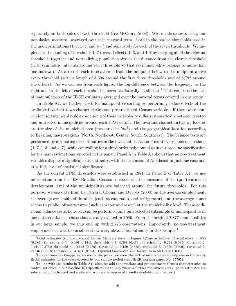
separately on both sides of each threshold (see McCrary, 2008). We run these tests using our
population measure—averaged over each mayoral term—both in the pooled thresholds used in
the main estimations (1–7, 1–3, and 4–7) and separately for each of the seven thresholds. We im-
plement the pooling of thresholds 1–7 (overall effect), 1–3, and 4–7 by merging all of the relevant
thresholds together and normalizing population size as the distance from the closest threshold
(with symmetric intervals around each threshold so that no municipality belongs to more than
one interval). As a result, each interval runs from the midpoint below to the midpoint above
every threshold (with a length of 3,396 around the first three thresholds and of 6,792 around
the others). As we can see from each figure, the log-difference between the frequency to the
right and to the left of each threshold is never statistically significant.2 This confirms the lack
of manipulation of the IBGE estimates averaged over the mayoral terms covered in our study.3
In Table A1, we further check for manipulative sorting by performing balance tests of the
available invariant town characteristics and pre-treatment Census variables. If there were non-
random sorting, we should expect some of these variables to differ systematically between treated
and untreated municipalities around each FPM cutoff. The invariant characteristics we look at
are the size of the municipal area (measured in km2) and the geographical location according
to Brazilian macro-regions (North, Northeast, Center, South, Southeast). The balance tests are
performed by estimating discontinuities in the invariant characteristics at every pooled threshold
(1–7, 1–3, and 4–7), while controlling for a third-order polynomial as in our baseline specification
for the main estimations reported in the paper. Panel A in Table A1 shows that no pre-treatment
variables display a significant discontinuity, with the exclusion of Northeast in just one case and
at a 10% level of statistical significance.
As the current FPM thresholds were established in 1981, in Panel B of Table A1, we use
information from the 1980 Brazilian Census to check whether measures of the (pre-treatment)
development level of the municipalities are balanced around the future thresholds. For this
purpose, we use data from La Ferrara, Chong, and Duryea (2008) on the average employment,
the average ownership of durables (such as car, radio, and refrigerator), and the average house
access to public infrastructures (such as water and sewer) at the municipality level. These addi-
tional balance tests, however, can be performed only on a selected subsample of municipalities in
our dataset, that is, those that already existed in 1980. From the original 2,877 municipalities
in our large sample, we thus end up with 2,276 observations. Importantly, no pre-treatment
employment or wealth variables show a significant discontinuity in this sample.4
2Point estimates (standard errors) for the McCrary tests in Figure A2 are as follows. Overall effect: -0.050(0.189); thresholds 1–3: -0.036 (0.144); thresholds 4–7: 0.391 (0.473); threshold 1: -0.213 (0.335); threshold 2:0.444 (0.375); threshold 3: -0.192 (0.270); threshold 4: 0.159 (0.328); threshold 5: 0.578 (0.609); threshold 6:-0.546 (0.719); threshold 7: -0.511 (0.924). Optimal bandwidth and binsize as in McCrary (2008).
3In a previous working-paper version of the paper, we show the lack of manipulative sorting also in the yearlyIBGE estimates for the years covered by our sample period (see NBER working paper No. 15705).
4In line with the results in Table A1, when we add the invariant and pre-treatment Census characteristics ascontrol variables in our baseline RD specifications to implement a further robustness check, point estimates aresubstantially unchanged and statistical accuracy is improved (results available upon request).
6

Finally, in Table A2, using the same specifications of Table A1, we run balance tests of
potentially endogenous variables at the FPM cutoffs. Specifically, we check whether the political
party of the mayor or his/her campaign funds (divided according to their source) display any
discontinuity. This is not a pre-requisite for the validity of our RD setup, but showing that
political orientation and campaign financing do not depend on FPM would rule out alternative
political mechanisms behind the baseline results. This is indeed the case, as no variable in Table
A2 shows any significant discontinuity. These findings are also discussed in the paper.
7

Figure A1 – Population distribution (below 50,941)
100
200
300
400
Frequency
10189 13585 16981 23773 30565 37356 44148
Population size
bin=1,132 bin=566
bin=283
Notes. Frequency of cities according to population size. Cities below 50,941 inhabitants only. The vertical lines identify theseven FPM revenue-sharing thresholds used in the empirical analysis of the paper. Mayoral terms 2001–2005 and 2005–2009.
8

Figure A2 – McCrary density tests: pooled and individual thresholds
1-7
.0001.0002.0003.0004.0005
-2000 -1000 0 1000 2000
1-3
.0001.0002.0003.0004.0005
-2000 -1000 0 1000 2000
4-7
0.0001.0002.0003.0004.0005
-2000 -1000 0 1000 2000
1
.0001.0002.0003.0004.0005
-2000 -1000 0 1000 2000
2
0.0001.0002.0003.0004.0005
-2000 -1000 0 1000 2000
3
0.00005.0001.00015.0002.00025
-4000 -2000 0 2000 4000
4
0.00005.0001.00015.0002.00025
-4000 -2000 0 2000 4000
5
0.0001
.0002
.0003
-4000 -2000 0 2000 4000
6
0.00005.0001.00015.0002.00025
-4000 -2000 0 2000 4000
7
0.0001.0002.0003.0004
-4000 -2000 0 2000 4000
Notes. Weighted kernel estimation of the log density (according to population size), performed separately on either side of eachpooled (1–7, 1–3, and 4–7) or individual FPM revenue-sharing threshold. Optimal binwidth and binsize as in McCrary (2008).Large sample with political selection variables. Mayoral terms 2001–2005 and 2005–2009.
9

Table A1 – Balance tests of invariant and pre-treatment characteristics
Overall effect Thresholds 1–3 Thresholds 4–7
A. Invariant town characteristics
Area size 2.367 1.177 8.983(4.605) (3.181) (15.164)
North -0.014 0.027 -0.060(0.022) (0.029) (0.044)
Northeast -0.009 -0.102* 0.096(0.039) (0.052) (0.075)
Center 0.004 0.007 -0.022
(0.020) (0.028) (0.037)Southeast -0.008 0.037 -0.105
(0.036) (0.048) (0.070)South 0.027 0.031 0.090
(0.029) (0.040) (0.055)
Obs. 2,877 1,979 898
B. Pre-treatment Census characteristics
Employed 0.195 -0.054 0.004(0.531) (0.711) (0.924)
Refrigerator 0.015 0.055 -0.337(0.463) (0.590) (0.992)
Radio 0.207 0.491 -0.224(0.362) (0.482) (0.769)
Car -0.032 -0.006 -0.209
(0.195) (0.248) (0.430)Water & sewer -0.265 -0.231 -0.753
(0.441) (0.546) (1.000)
Obs. 2,276 1,682 594Notes. Estimated discontinuity of invariant town characteristics (panel A) and pre-treatment Cen-sus characteristics (panel B) at the FPM thresholds. Each cell reports the estimated coefficient of a
dummy equal to one (zero) if population size is above (below) the closest threshold—controlling for athird-order polynomial in normalized population size, term dummies, and macro-region dummies—
in a regression where the dependent variable corresponds to each row heading. Robust standarderrors clustered at the municipality level are in parentheses. The column “Overall effect” is ob-
tained by estimations in the entire sample (i.e., thresholds 1–7); the columns “Thresholds 1-3”and “Thresholds 4-7” are obtained by estimations in the respective subsamples. Invariant town
characteristics: area size is expressed in km2; North, Northeast, Center, Southeast, and South aregeographic location dummies. Pre-treatment Census characteristics: all variables come from the
1980 Census, are per capita, and refer to average employment; refrigerator, radio, or car ownership;house access to water and sewer. Mayoral terms 2001–2005 and 2005–2009. Significance at the
10% level is represented by *, at the 5% level by **, and at the 1% level by ***.
10
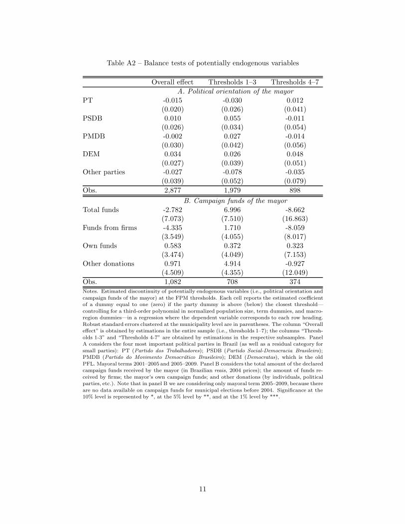
Table A2 – Balance tests of potentially endogenous variables
Overall effect Thresholds 1–3 Thresholds 4–7
A. Political orientation of the mayor
PT -0.015 -0.030 0.012(0.020) (0.026) (0.041)
PSDB 0.010 0.055 -0.011(0.026) (0.034) (0.054)
PMDB -0.002 0.027 -0.014(0.030) (0.042) (0.056)
DEM 0.034 0.026 0.048
(0.027) (0.039) (0.051)Other parties -0.027 -0.078 -0.035
(0.039) (0.052) (0.079)
Obs. 2,877 1,979 898
B. Campaign funds of the mayor
Total funds -2.782 6.996 -8.662(7.073) (7.510) (16.863)
Funds from firms -4.335 1.710 -8.059(3.549) (4.055) (8.017)
Own funds 0.583 0.372 0.323(3.474) (4.049) (7.153)
Other donations 0.971 4.914 -0.927(4.509) (4.355) (12.049)
Obs. 1,082 708 374Notes. Estimated discontinuity of potentially endogenous variables (i.e., political orientation and
campaign funds of the mayor) at the FPM thresholds. Each cell reports the estimated coefficientof a dummy equal to one (zero) if the party dummy is above (below) the closest threshold—
controlling for a third-order polynomial in normalized population size, term dummies, and macro-region dummies—in a regression where the dependent variable corresponds to each row heading.
Robust standard errors clustered at the municipality level are in parentheses. The column “Overalleffect” is obtained by estimations in the entire sample (i.e., thresholds 1–7); the columns “Thresh-
olds 1-3” and “Thresholds 4-7” are obtained by estimations in the respective subsamples. PanelA considers the four most important political parties in Brazil (as well as a residual category for
small parties): PT (Partido dos Trabalhadores); PSDB (Partido Social-Democracia Brasileiro);PMDB (Partido do Movimento Democratico Brasileiro); DEM (Democratas), which is the old
PFL. Mayoral terms 2001–2005 and 2005–2009. Panel B considers the total amount of the declaredcampaign funds received by the mayor (in Brazilian reais, 2004 prices); the amount of funds re-
ceived by firms; the mayor’s own campaign funds; and other donations (by individuals, politicalparties, etc.). Note that in panel B we are considering only mayoral term 2005–2009, because there
are no data available on campaign funds for municipal elections before 2004. Significance at the10% level is represented by *, at the 5% level by **, and at the 1% level by ***.
11

A3 Examples of violation episodes from the audit reports
Illegal procurement practices
(a) Limited competition. In the municipality of Buritis (state of Rondonia), in a bidding
process regarding the purchase of food, the city invited three companies, two of them from the
municipality of Porto Velho, 210 kilometers far from Buritis. Auditors contested this fact because
in Buritis there are companies that could have participated in the auction. More importantly,
the company that won the bid for all 64 items (42,000 reais) was owned by the mayor’s wife.
The mayor’s wife was also the accountant of another company that was invited to participate
in the auction.
(b) Manipulation of the bid value. In the municipality of Itapira (state of Sao Paulo),
auditors found evidence of manipulation of the bid value for the acquisition of materials in the
construction of the water supply system. According to Law No. 8666/93, if the value of the
project is below a certain threshold, no bid process is required. Auditors found evidence that
the municipal administration had divided the project into three (fake) sub-projects in order to
avoid the bid procedure.
Fraud
In the municipality of Santa Terezinha (state of Bahia), auditors found evidence of a simu-
lated auction for the purchase of computer equipment worth about 10,000 reais. The companies
alleged to have participated in the procurement practice were: LL Equipmentos Informatica
Ltda. (winner), MSGL Informatica Ltda., Nucleo Comercio, and Servicos de Informatica Ltda.
Although it is required that all bidders attend the opening of the tender envelopes, the company
MSGL Informatica Ltda. never participated to the auction. The director of the winning com-
pany (LL Equipmentos) declared to the auditors that: “(...) I sold computer equipment worth
10,000 reais to the municipality of Santa Teresinha, represented by the mayor’s husband, who
showed me two different proposals by other companies and asked me to under-bid them.”
In the municipality of Salinas da Margarida (state of Bahia), there was evidence of a sim-
ulated auction involving funds for education (FUNDEF): in three bidding processes for a total
amount of 142,600 reais, the alleged participants denied any involvement in the auction. For
example, the owners of the companies Plantek and J.S. Construcoes Gerais formally declared to
the auditors that they had not been called to the auction and their signatures had been falsified.
Favoritism in the good receipt
In the municipality of General Sampaio (state of Ceara), auditors found out that the land
on which a dam was built had been previously donated by the city to the owner, and that this
person also owned the surrounding areas, hampering free access to the dam.
12

Over-invoicing
In the municipality of Sao Fransciso do Conde (state of Bahia), the construction company
Mazda was hired without a bidding process to carry out the construction of a road nine kilometers
long. The road should have been budgeted at about 1 million reais, but the invoices presented
by the company proved that there had been a disbursement of 5 million reais. The municipal
administration did not present any document justifying the expenditure. Mazda, a company
with no experience in road construction, sub-contracted another company to perform the job
only paying 1,800,000 reais.
Diversion of funds
The municipality of Buritis (state of Rondonia) received 50,000 reais from the federal gov-
ernment to purchase a school bus for transporting students. Auditors found that the vehicle was
also used to transport professors from the urban area to schools in rural areas. Furthermore,
the school bus performed trips outside the municipality without justification.
In the municipality of Candido Mendes (state of Maranhao), 91% of the resources that
should have been spent for the salaries of professors were actually used to pay public employees
performing different duties.
In the municipality of Belem (state of Paraıba), auditors found out that 160,000 reais that
should have been spent on basic health services (i.e., medical consultations, basic dental care,
vaccinations, educational activities, etc.) were used to pay meals for the staff of the health
program and to cover debt services of the municipality.
Paid but not proven
The municipality of Cerro Branco (state of Rio Grande do Sul ) did not provide any docu-
mentation to justify the expenditure of 29,100 reais for health services.
13
A4 Robustness checks
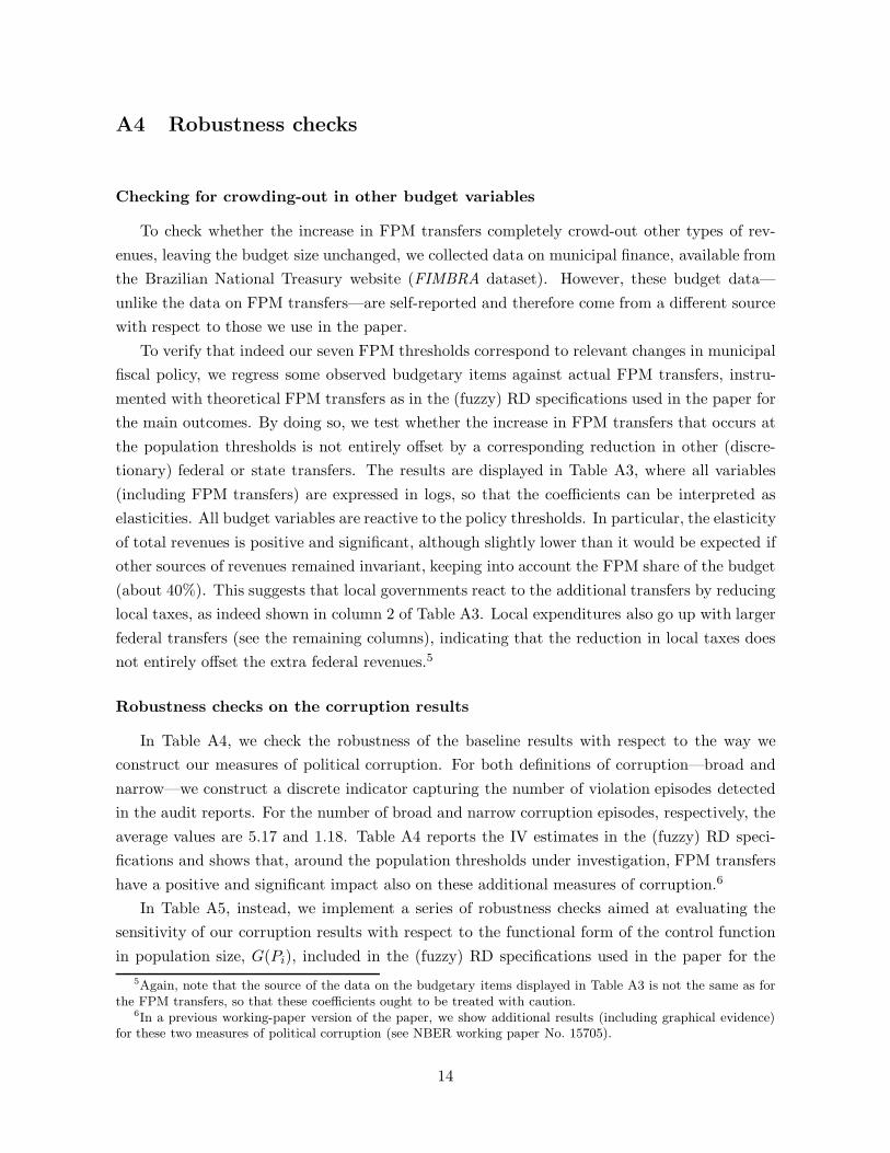
Checking for crowding-out in other budget variables
To check whether the increase in FPM transfers completely crowd-out other types of rev-
enues, leaving the budget size unchanged, we collected data on municipal finance, available from
the Brazilian National Treasury website (FIMBRA dataset). However, these budget data—
unlike the data on FPM transfers—are self-reported and therefore come from a different source
with respect to those we use in the paper.
To verify that indeed our seven FPM thresholds correspond to relevant changes in municipal
fiscal policy, we regress some observed budgetary items against actual FPM transfers, instru-
mented with theoretical FPM transfers as in the (fuzzy) RD specifications used in the paper for
the main outcomes. By doing so, we test whether the increase in FPM transfers that occurs at
the population thresholds is not entirely offset by a corresponding reduction in other (discre-
tionary) federal or state transfers. The results are displayed in Table A3, where all variables
(including FPM transfers) are expressed in logs, so that the coefficients can be interpreted as
elasticities. All budget variables are reactive to the policy thresholds. In particular, the elasticity
of total revenues is positive and significant, although slightly lower than it would be expected if
other sources of revenues remained invariant, keeping into account the FPM share of the budget
(about 40%). This suggests that local governments react to the additional transfers by reducing
local taxes, as indeed shown in column 2 of Table A3. Local expenditures also go up with larger
federal transfers (see the remaining columns), indicating that the reduction in local taxes does
not entirely offset the extra federal revenues.5
Robustness checks on the corruption results
In Table A4, we check the robustness of the baseline results with respect to the way we
construct our measures of political corruption. For both definitions of corruption—broad and
narrow—we construct a discrete indicator capturing the number of violation episodes detected
in the audit reports. For the number of broad and narrow corruption episodes, respectively, the
average values are 5.17 and 1.18. Table A4 reports the IV estimates in the (fuzzy) RD speci-
fications and shows that, around the population thresholds under investigation, FPM transfers
have a positive and significant impact also on these additional measures of corruption.6
In Table A5, instead, we implement a series of robustness checks aimed at evaluating the
sensitivity of our corruption results with respect to the functional form of the control function
in population size, G(Pi), included in the (fuzzy) RD specifications used in the paper for the
5Again, note that the source of the data on the budgetary items displayed in Table A3 is not the same as forthe FPM transfers, so that these coefficients ought to be treated with caution.
6In a previous working-paper version of the paper, we show additional results (including graphical evidence)for these two measures of political corruption (see NBER working paper No. 15705).
14

main outcomes. In particular, we specify G(Pi) as either a spline third-order polynomial (with
each interval going from a midpoint to the next), a second-order polynomial (spline or not), or a
fourth-order polynomial (spline or not): in all of these cases, the results are very similar to those
found in the baseline specification with a third-order polynomial (see Table 5 in the paper).
Robustness checks on the political selection results
In Table A6, we implement a series of robustness checks to evaluate the sensitivity of our
political selection results with respect to the functional form of G(Pi), as we have done for the
corruption results in Table A5. Again, the results are strongly robust to any specification of the
functional form of the control function in population size.
Finally, in Table A7, we check whether the political selection results depend on the fact that—
in order to stay close to our theoretical framework—we restrict the sample to municipalities
where the incumbent runs for reelection. This is not the case, because the same negative
impact of FPM transfers on the educational level of politicians is detected when considering all
mayoral candidates in Brazilian municipalities over the terms considered in the paper (sample
A); only the opponents (of the incumbent who runs for reelection) with the highest number of
votes (sample B); all political candidates in municipalities where the incumbent does not run
for reelection and all opponents in municipalities where the incumbent reruns (sample C); and
all the opponents of the political party of the incumbent mayor, irrespective of whether the
incumbent reruns or not (sample D). On the whole, the results on the educational attainments
of politicians are strongly robust to these alternative sample selection choices.7
7As discussed in the paper, mayors are the crucial players in Brazilian municipal governments and corruptionepisodes detected by the audit reports refer to the municipal government, not to the municipal legislature (i.e.,City Council). However, the same negative effect of FPM transfers on the quality of politicians is detected whenlooking at the educational level of city councillors. In particular, the impact of transfers on the college dummy isnot statistically different from zero, but the impact on years of schooling is positive and statistically significant:point estimates (standard errors) are as follows. Overall effect: -0.023 (0.010); thresholds 1–3: -0.034 (0.015);thresholds 4–7: -0.015 (0.010); threshold 1: -0.048 (0.028); threshold 2: -0.084 (0.024); threshold 3: -0.038 (0.018);threshold 4: -0.035 (0.016); threshold 5: -0.026 (0.015); threshold 6: -0.013 (0.014); threshold 7: -0.022 (0.017).
15

Table A3 – IV estimates: budget variables
Total Local Total Infrastructure Personnel
revenues taxes expenditure expenditure expenditure
Overall effect 0.527*** -0.623*** 0.473*** 0.618*** 0.362***(0.107) (0.238) (0.109) (0.237) (0.114)
Thresholds 1–3 0.019*** -0.023** 0.018*** 0.028*** 0.012***(0.004) (0.010) (0.004) (0.008) (0.005)
Thresholds 4–7 0.004 -0.020*** 0.002 0.012** -0.004(0.003) (0.007) (0.003) (0.006) (0.003)
Threshold 1 0.037*** -0.029* 0.035*** 0.052*** 0.030***
(0.007) (0.016) (0.007) (0.016) (0.008)Threshold 2 0.024*** -0.033** 0.022*** 0.033** 0.015**
(0.007) (0.014) (0.007) (0.013) (0.008)Threshold 3 0.020*** -0.013 0.019*** 0.034*** 0.012**
(0.005) (0.012) (0.005) (0.010) (0.006)Threshold 4 0.010** -0.020* 0.008* 0.017* -0.003
(0.005) (0.011) (0.005) (0.009) (0.006)
Threshold 5 0.014** -0.011 0.011* 0.034*** 0.004(0.006) (0.013) (0.006) (0.011) (0.007)
Threshold 6 0.002 -0.022** 0.002 0.008 -0.001(0.004) (0.011) (0.004) (0.008) (0.004)
Threshold 7 0.002 -0.033** 0.000 0.005 -0.006(0.006) (0.013) (0.006) (0.011) (0.007)
Obs. 2,877 2,877 2,877 2,877 2,877Notes. Effects of FPM transfers on other budget variables. Each cell reports the estimated coefficient of actual FPM transfers
(instrumentedwith theoreticalFPM transfers)—controlling for a third-order polynomial in normalized population size, termdummies, and macro-region dummies—in a regression where the dependent variable corresponds to each column heading.
Robust standard errors clustered at the municipality level are in parentheses. The coefficients in the row “Thresholds1-7” are obtained by estimating the regression in the entire sample; the heterogeneity coefficients in the other rows are
obtained by interacting the regression with population-interval dummies (from the midpoint below to the midpoint aboveFPM thresholds) for “Thresholds 1-3,” “Thresholds 4-7,” and each individual threshold, respectively. All variables are in
logs; the original budget variables are expressed in Brazilian reais at 2000 prices. Mayoral terms 2001–2005 and 2005–2009.Significance at the 10% level is represented by *, at the 5% level by **, and at the 1% level by ***.
16

Table A4 – IV estimates: additional corruption measures
Number of Number of
broad corruption narrow corruptionepisodes episodes
Overall effect 0.311** 0.108***
(0.125) (0.034)Thresholds 1–3 0.313** 0.145***
(0.148) (0.047)Thresholds 4–7 0.383** 0.100**
(0.159) (0.041)
Threshold 1 0.036 0.060(0.227) (0.067)
Threshold 2 0.327 0.119**(0.202) (0.060)
Threshold 3 0.371* 0.149**(0.198) (0.063)
Threshold 4 0.223 0.066
(0.218) (0.053)Threshold 5 0.774** 0.141*
(0.309) (0.075)Threshold 6 0.286* 0.095*
(0.173) (0.053)Threshold 7 0.049 0.010
(0.226) (0.054)
Obs. 1,202 1,202Notes. Effects of FPM transfers on additional corruption measures. Each cell reports the es-timated coefficient of actual FPM transfers (instrumented with theoretical FPM transfers)—
controlling for a third-order polynomial in normalized population size, term dummies, andmacro-region dummies—in a regression where the dependent variable corresponds to each
column heading. Robust standard errors clustered at the municipality level are in parenthe-ses. The coefficients in the row “Thresholds 1-7” are obtained by estimating the regression
in the entire sample; the heterogeneity coefficients in the other rows are obtained by in-teracting the regression with population-interval dummies (from the midpoint below to the
midpoint above FPM thresholds) for “Thresholds 1-3,” “Thresholds 4-7,” and each indi-vidual threshold, respectively. The additional measures of corruption are only available for
the small sample (random audit reports): number of broad corruption episodes and number
of narrow corruption episodes measure the number of episodes linked to general or serious
violations, respectively. Mayoral terms 2001–2005 and 2005–2009. Significance at the 10%
level is represented by *, at the 5% level by **, and at the 1% level by ***.
17
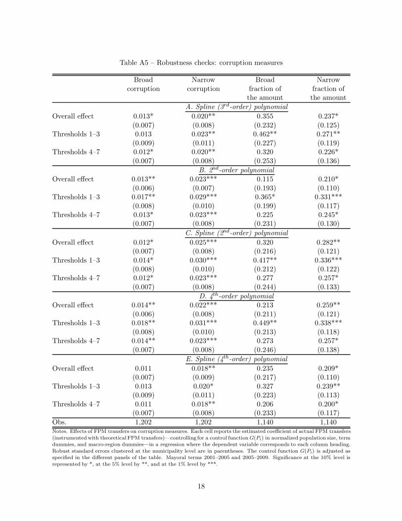
Table A5 – Robustness checks: corruption measures
Broad Narrow Broad Narrow
corruption corruption fraction of fraction ofthe amount the amount
A. Spline (3rd-order) polynomial
Overall effect 0.013* 0.020** 0.355 0.237*
(0.007) (0.008) (0.232) (0.125)Thresholds 1–3 0.013 0.023** 0.462** 0.271**
(0.009) (0.011) (0.227) (0.119)Thresholds 4–7 0.012* 0.020** 0.320 0.226*
(0.007) (0.008) (0.253) (0.136)
B. 2nd-order polynomial
Overall effect 0.013** 0.023*** 0.115 0.210*
(0.006) (0.007) (0.193) (0.110)Thresholds 1–3 0.017** 0.029*** 0.365* 0.331***
(0.008) (0.010) (0.199) (0.117)Thresholds 4–7 0.013* 0.023*** 0.225 0.245*
(0.007) (0.008) (0.231) (0.130)
C. Spline (2nd-order) polynomial
Overall effect 0.012* 0.025*** 0.320 0.282**(0.007) (0.008) (0.216) (0.121)
Thresholds 1–3 0.014* 0.030*** 0.417** 0.336***(0.008) (0.010) (0.212) (0.122)
Thresholds 4–7 0.012* 0.023*** 0.277 0.257*
(0.007) (0.008) (0.244) (0.133)
D. 4th-order polynomial
Overall effect 0.014** 0.022*** 0.213 0.259**
(0.006) (0.008) (0.211) (0.121)Thresholds 1–3 0.018** 0.031*** 0.449** 0.338***
(0.008) (0.010) (0.213) (0.118)Thresholds 4–7 0.014** 0.023*** 0.273 0.257*
(0.007) (0.008) (0.246) (0.138)
E. Spline (4th-order) polynomial
Overall effect 0.011 0.018** 0.235 0.209*(0.007) (0.009) (0.217) (0.110)
Thresholds 1–3 0.013 0.020* 0.327 0.239**(0.009) (0.011) (0.223) (0.113)
Thresholds 4–7 0.011 0.018** 0.206 0.200*(0.007) (0.008) (0.233) (0.117)
Obs. 1,202 1,202 1,140 1,140Notes. Effects of FPM transfers on corruption measures. Each cell reports the estimated coefficient of actual FPM transfers
(instrumented with theoretical FPM transfers)—controlling for a control function G(Pi) in normalized population size, termdummies, and macro-region dummies—in a regression where the dependent variable corresponds to each column heading.
Robust standard errors clustered at the municipality level are in parentheses. The control function G(Pi) is adjusted asspecified in the different panels of the table. Mayoral terms 2001–2005 and 2005–2009. Significance at the 10% level is
represented by *, at the 5% level by **, and at the 1% level by ***.
18

Table A6 – Robustness checks: opponents’ education and election outcome
College Years Incumbent
of schooling reelection
A. Spline (3rd-order) polynomial
Overall effect -0.009** -0.078*** 0.009(0.004) (0.030) (0.005)
Thresholds 1–3 -0.019*** -0.165*** 0.013*(0.007) (0.047) (0.008)
Thresholds 4–7 -0.007* -0.060** 0.008(0.004) (0.029) (0.005)
B. 2nd-order polynomial
Overall effect -0.006* -0.065*** 0.012***(0.004) (0.025) (0.004)
Thresholds 1–3 -0.017*** -0.150*** 0.014**(0.006) (0.040) (0.007)
Thresholds 4–7 -0.006* -0.052** 0.009*(0.004) (0.026) (0.005)
C. Spline (2nd-order) polynomial
Overall effect -0.009** -0.073** 0.009*
(0.004) (0.029) (0.005)Thresholds 1–3 -0.016*** -0.146*** 0.013*
(0.006) (0.043) (0.007)Thresholds 4–7 -0.006 -0.052* 0.008
(0.004) (0.027) (0.005)
D. 4th-order polynomial
Overall effect -0.009** -0.078*** 0.012***(0.004) (0.026) (0.005)
Thresholds 1–3 -0.018*** -0.158*** 0.014**(0.006) (0.042) (0.007)
Thresholds 4–7 -0.007* -0.059** 0.009*(0.004) (0.027) (0.005)
E. Spline (4th-order) polynomial
Overall effect -0.007 -0.068** 0.009
(0.005) (0.031) (0.006)Thresholds 1–3 -0.015** -0.146*** 0.013
(0.007) (0.049) (0.008)Thresholds 4–7 -0.006 -0.057* 0.008
(0.005) (0.030) (0.005)
Obs. 2,877 2,877 2,877Notes. Effects of FPM transfers on the opponents’ education and election outcome. Each cell reports theestimated coefficient of actual FPM transfers (instrumented with theoretical FPM transfers)—controlling
for a control function G(Pi) in normalized population size, term dummies, and macro-region dummies—ina regression where the dependent variable corresponds to each column heading. Robust standard errors
clustered at the municipality level are in parentheses. The control function G(Pi) is adjusted as specified
in the different panels of the table. Mayoral terms 2001–2005 and 2005–2009. Significance at the 10%level is represented by *, at the 5% level by **, and at the 1% level by ***.
19

Table A7 – IV estimates: politicians’ education in different samples
College Years of College Years of College Years of College Years of
schooling schooling schooling schooling
Sample A Sample B Sample C Sample DOverall effect -0.003 -0.059*** -0.011** -0.089*** -0.004 -0.063*** -0.004 -0.058***
(0.003) (0.018) (0.005) (0.032) (0.003) (0.019) (0.003) (0.020)Thresholds 1–3 -0.010** -0.106*** -0.020*** -0.175*** -0.011*** -0.115*** -0.011*** -0.118***
(0.004) (0.028) (0.007) (0.0052) (0.004) (0.029) (0.004) (0.030)Thresholds 4–7 -0.003 -0.045** -0.011** -0.076** -0.004 -0.051*** -0.004 -0.049**
(0.003) (0.019) (0.007) (0.034) (0.003) (0.019) (0.003) (0.020)
Threshold 1 -0.005 -0.086* -0.022* -0.221** -0.005 -0.089* -0.004 -0.093*(0.007) (0.052) (0.012) (0.096) (0.007) (0.053) (0.007) (0.055)
Threshold 2 -0.013** -0.163*** -0.027** -0.244*** -0.015** -0.179*** -0.016** -0.192***(0.006) (0.043) (0.011) (0.080) (0.006) (0.045) (0.007) (0.047)
Threshold 3 -0.010** -0.082*** -0.022** -0.163*** -0.011** -0.093*** -0.011** -0.095***(0.005) (0.032) (0.009) (0.059) (0.005) (0.032) (0.005) (0.033)
Threshold 4 -0.004 -0.053* -0.011 -0.064 -0.005 -0.063** -0.005 -0.059*
(0.004) (0.029) (0.008) (0.059) (0.004) (0.030) (0.005) (0.032)Threshold 5 -0.001 -0.042 -0.012 -0.103* -0.002 -0.046 -0.000 -0.046
(0.004) (0.030) (0.008) (0.053) (0.005) (0.030) (0.005) (0.031)Threshold 6 -0.005 -0.064** -0.012 -0.089** -0.005 -0.066** -0.008* -0.080***
(0.004) (0.026) (0.008) (0.043) (0.004) (0.026) (0.004) (0.028)Threshold 7 0.004 0.003 -0.010 -0.089* 0.003 -0.004 0.005 0.004
(0.004) (0.028) (0.008) (0.052) (0.004) (0.029) (0.004) (0.029)
Obs. 5,648 5,648 2,788 2,788 5,452 5,452 5,281 5,281Notes. Effects of FPM transfers on the education of political candidates in different samples. Each cell reports the estimated coefficient of actual FPM transfers (instrumentedwith theoretical FPM transfers)—controlling for a third-order polynomial in normalized population size, term dummies, and macro-region dummies—in a regression where
the dependent variable corresponds to each column heading. Robust standard errors clustered at the municipality level are in parentheses. The coefficients in the row“Overall effect” are obtained by estimating the regression in the entire sample (i.e., thresholds 1-7); the heterogeneity coefficients in the other rows are obtained by
interacting the regression with population-interval dummies (from the midpoint below to the midpoint above FPM thresholds) for “Thresholds 1-3,” “Thresholds 4-7,” andeach individual threshold, respectively. Sample A considers all political candidates in all municipalities. Sample B considers only the opponents (of the incumbent who
runs for reelection) with the highest number of votes. Sample C considers all political candidates in municipalities where the incumbent does not run for reelection and allopponents in municipalities where the incumbent reruns. Sample D considers all the opponents of the political party of the incumbent mayor (irrespective of whether the
incumbent reruns or not). Mayoral terms 2001–2005 and 2005–2009. Significance at the 10% level is represented by *, at the 5% level by **, and at the 1% level by ***.