2010-2012 california household travel survey final...
TRANSCRIPT

California Department of Transportation
2010-2012 California Household Travel Survey Final Report
June 2013
Contact: Martin Kunzmann, Project Manager
206 Wild Basin Road, Building A, Suite 300, Austin, Texas 78746,Phone: 512-306-9065
In Association with: GeoStats Franklin Hill Group Mark Bradley Research & Consulting

Acknowledgements – Funding, Administrative, Steering and Technical Advisory Committees Oversight of the CHTS was provided by two main committees, the Administrative Committee (AC) and the Steering Committee (SC) along with several Technical Advisory Committees (TAC). Also, Caltrans would like to acknowledge support of its funding partners for making this project to happen. Funding Partners are:
• California Energy Commission • Kern Council of Governments • Strategic Growth Council • Metropolitan Transportation Commission • Southern California Association of Governments • Association of Monterey Bay Area Governments • San Joaquin Valley Air Pollution Control District: • Santa Barbara County Association of Governments • Tulare County Association of Governments
The AC consisted of the following individuals: Vahid Nowshiravan, Caltrans Peter Spaulding, Caltrans Sarah Chesebro, Caltrans Soheila Khoii, Caltrans Mike Ainsworth, SCAG Rahul Srivastava, Caltrans Kalin Pacheco, Caltrans Rochelle Invina, KernCOG Shimon Israel, MTC David Ory, MTC Bruce Griesenbeck, SACOG Julio Perucho, SBCAG Peter Imhof, SBCAG James Worthley, SLOCOG Ed Flickinger, KernCOG Troy Hightower, KernCOG Robert Ball, KernCOG Bhupendra Patel, AMBAG Mark Hays, Tulare Kim Kloeb, SJCOG Carlos Yamzon, STANCOG Jim Schoeffling, STANCOG Mike Bitner, FresnoCOG Aniss Bahreinian, California Energy Commission Ron West, Cambridge Systematics Mark Bradley, Mark Bradley Research and Consulting Kostas Goulias, Morrison & Goulias

Aditya Katragadda, NuStats Sandra Rodriguez, NuStats Sue Foster, NuStats Vivian Masterman, NuStats Sujin Hong, NuStats Martin Kunzmann, NuStats Cheryl Stecher, Franklin Hill Group Alison Boehm, GeoStats Glenn Frankel, GeoStats Jean Wolf, GeoStats Jeremy Wilhelm, GeoStats Joel Anders, GeoStats Laura Lyons, GeoStats Laura Wilson, GeoStats Marcelo Oliveira, GeoStats Michael Mitchell, GeoStats Michelle Lee, GeoStats The SC consisted of the following individuals: Bhupendra Patel, AMBAG Brian Lasagna, BCAG Bruce Griesenbeck, SACOG Carlos Yamzon, STANCOG Charles Field, ACTC-Amador Clint Daniels, SANDAG David Ory, MTC Derek Winning, MaderaCTC Ed Flickinger, KernCOG Huang Guoxiong, SCAG James Worthley, SLOCOG Jim Schoeffling, STANCOG Joanne Marchetta, TRPA Julio Perucho, SBCAG Kai Han, FresnoCOG Kim Kloeb, SJCOG Kristin Cai, FresnoCOG Mark Hays, Tulare Matt Fell, MCA Mike Bitner, FresnoCOG Nick Haven, TRPA Paul Burke, Metro Peter Imhof, SBCAG Randy Deshazo, AMBAG Rick Curry, SANDAG Robert Farley, Metro Robert Ball, KernCOG Sean Tiedgen, SRTA Yongping Zhang, SCAG Shimon Israel, MTC Troy Hightower, KernCOG

Wu Sun, SANDAG Yongping Zhang, SCAG Anda Graghici, Housing and Community Development Aniss Bahreinian, California Energy Commission Bob McBride, California Energy Commission Glen Campora, Housing and Community Development Greg Harris, Air Resources Board Jeff Long, Air Resources Board Jon Taylor, Air Resources Board Linda Wheaton, Housing and Community Development Nesamani Kalandiyur, Air Resources Board Todd Sax, Air Resources Board YanPing Zuo, Air Resources Board Zhen Dai, Air Resources Board Doug Hunt, University of Calgary Kostas Goulias, Morrison & Goulias Mike McCoy, UC Davis Susan Handy, UC Davis Kalin Pacheco, Caltrans Vahid Nowshiravan, Caltrans Peter Spaulding, Caltrans Sarah Chesebro, Caltrans Soheila Khoii, Caltrans Mike Ainsworth, SCAG Al Arana, Caltrans Chad Baker, Caltrans Cynthia Smith, Caltrans David Berggren, Caltrans Diana Portillo, Caltrans Doug MacIvor, Caltrans Emily Burstein, Caltrans Leonard Seitz, Caltrans Mohammad Assadi, Caltrans Tami Cuccia, Caltrans Ron West, Cambridge Systematics Mark Bradley, Mark Bradley Research and Consulting Aditya Katragadda, NuStats Sandra Rodriguez, NuStats Sue Foster, NuStats Vivian Masterman, NuStats Sujin Hong, NuStats Martin Kunzmann, NuStats Cheryl Stecher, Franklin Hill Group Elaine Murakami, FHWA Georgiena Vivian, VRPA Technologies Alison Boehm, GeoStats Glenn Frankel, GeoStats Jean Wolf, GeoStats Jeremy Wilhelm, GeoStats Joel Anders, GeoStats Laura Lyons, GeoStats

Laura Wilson, GeoStats Marcelo Oliveira, GeoStats Michael Mitchell, GeoStats Michelle Lee, GeoStats The TAC for Hard to Reach Populations consisted of the following individuals: Laurie Wargelin, Abt SRBI Angela Rushen, SCAG Brenda Kahn, MTC Craig Noble, MTC Ellen Griffin, MTC Leslie Lara, MTC Terry Lee, MTC Sandy Louey, California Energy Commission Bhupendra Patel, AMBAG Kim Kloeb, SJCOG Mark Hays, Tulare Mike Bitner, FresnoCOG Paul Burke, Metro Shimon Israel, MTC Troy Hightower, KernCOG Kostas Goulias, Morrison & Goulias Vahid Nowshiravan, Caltrans Sarah Chesebro, Caltrans Soheila Khoii, Caltrans Mike Ainsworth, SCAG Kalin Pacheco, Caltrans Diana Portillo, Caltrans Karen Brewster, Caltrans Mark Barry, Caltrans Matt Rocco, Caltrans Aditya Katragadda, NuStats Cheryl Stecher, Franklin Hill Group Claudia Rojo, NuStats Martin Kunzmann, NuStats Vivian Masterman, NuStats Elaine Murakami, FHWA Dena Graham, VRPA Technologies Erica Thompson, VRPA Technologies Georgiena Vivian, VRPA Technologies Alison Boehm, GeoStats Glenn Frankel, GeoStats Jean Wolf, GeoStats Jeremy Wilhelm, GeoStats Joel Anders, GeoStats Laura Lyons, GeoStats Laura Wilson, GeoStats Marcelo Oliveira, GeoStats Michael Mitchell, GeoStats Michelle Lee, GeoStats

The TAC for CHTS Long Distance & Inter-regional Trips consisted of the following individuals: Ed Flickinger, KernCOG Robert Farley, Metro Aniss Bahreinian, California Energy Commission Bob McBride, California Energy Commission Doug Hunt, University of Calgary Vahid Nowshiravan, Caltrans Peter Spaulding, Caltrans Sarah Chesebro, Caltrans Soheila Khoii, Caltrans Mike Ainsworth, SCAG Chad Baker, Caltrans Doug MacIvor, Caltrans Leonard Seitz, Caltrans Mark Bradley, Mark Bradley Research and Consulting Ron West, Cambridge Systematics Cheryl Stecher, Franklin Hill Group Sandra Rodriguez, NuStats Vivian Masterman, NuStats Sue Foster, NuStats Alison Boehm, GeoStats Glenn Frankel, GeoStats Jean Wolf, GeoStats Jeremy Wilhelm, GeoStats Joel Anders, GeoStats Laura Lyons, GeoStats Laura Wilson, GeoStats Marcelo Oliveira, GeoStats Michael Mitchell, GeoStats Michelle Lee, GeoStats The TAC for CHTS Data and Model Transferability consisted of the following individuals: Bhupendra Patel, AMBAG Ed Flickinger, KernCOG Huang Guoxiong, SCAG Robert Farley, Metro Yongping Zhang, SCAG Aniss Bahreinian, California Energy Commission Peter Spaulding, Caltrans Sarah Chesebro, Caltrans Soheila Khoii, Caltrans Mike Ainsworth, SCAG Doug MacIvor, Caltrans Leonard Seitz, Caltrans Mark Bradley, Mark Bradley Research and Consulting Ron West, Cambridge Systematics Cheryl Stecher, Franklin Hill Group Sandra Rodriguez, NuStats

i California Household Travel Survey Final Report Version 1.0
Table of Contents
1.0 Executive Summary ..............................................................................................................................1
1.1 Survey Overview ..............................................................................................................................1
1.2 Key Statewide Statistics ...................................................................................................................1
2.0 Introduction .........................................................................................................................................5
2.1 Survey Objectives and Overall Approach ........................................................................................5
2.2 Description of the Survey Components ...........................................................................................7
2.3 Survey Oversight Committees .........................................................................................................8
2.4 Survey Schedule ...............................................................................................................................8
3.0 Survey Design ..................................................................................................................................... 10
3.1 Survey Instrument and Materials Design ..................................................................................... 10
3.2 Sample Design............................................................................................................................... 13
3.2.1 Source of Sample and Survey Universe ........................................................................... 13
3.2.2 Sampling Design and Selection Methodology ................................................................. 13
3.2.3 Geographic Distribution................................................................................................... 15
4.0 Survey Methods ................................................................................................................................. 30
4.1 Survey Pretest ............................................................................................................................... 30
4.2 Final Survey Design ....................................................................................................................... 30
4.2.1 Main Survey Data Collection Overview ........................................................................... 31
4.2.2 Survey Processes ............................................................................................................. 32
4.2.3 Proxy Reporting ............................................................................................................... 36
4.2.4 Call Backs ......................................................................................................................... 36
4.2.5 Refusals ............................................................................................................................ 37
4.2.6 Hotline ............................................................................................................................. 37
4.2.7 Non-English Speaking Households .................................................................................. 38
4.2.8 Interviewer Training ........................................................................................................ 39
4.2.9 Incentives ......................................................................................................................... 39
4.2.10 Definition of a Completed Household ............................................................................. 41
4.2.11 Long Distance Logs .......................................................................................................... 42
4.2.12 Respondent Burden ......................................................................................................... 43
4.2.13 Sample Management ....................................................................................................... 43
4.3 Survey Outreach – Hard to Reach Populations ............................................................................ 45
4.4 Quality Control .............................................................................................................................. 46
5.0 Global Positioning System (GPS) Subsample ........................................................................................ 48
5.1 Overview ....................................................................................................................................... 48
5.2 Deployment Methods and Results ............................................................................................... 48
5.2.1 Deployment Methods ...................................................................................................... 48
5.2.2 Deployment Results ......................................................................................................... 51
5.2.3 GPS Participation Results ................................................................................................. 52

ii California Household Travel Survey Final Report Version 1.0
5.3 GPS/Diary Processing Methods and Results ................................................................................. 53
5.4 OBD Data Collection and Processing ............................................................................................ 55
5.5 GPS and Diary Trip Matching Results ........................................................................................... 60
5.5.1 Reporting Exceptions ....................................................................................................... 60
5.5.2 Matching Results - Wearable ........................................................................................... 61
5.5.3 Matching Results – Vehicle .............................................................................................. 64
5.5.4 Matching Results – Vehicle / OBD ................................................................................... 66
5.5.5 Matching Results – Summary Tables ............................................................................... 68
5.6 Link Matching................................................................................................................................ 69
5.6.1 Process Description ......................................................................................................... 69
5.7 GPS Data Deliverables................................................................................................................... 71
6.0 Assessment of Survey Quality ............................................................................................................. 72
6.1 Item Non-Response Analysis ........................................................................................................ 72
6.2 Expected Value Ranges and Logical Relationships between Items .............................................. 74
6.3 Geographic Coverage .................................................................................................................... 77
6.4 Response Rate Summary .............................................................................................................. 79
6.4.1 Total Sample Size ............................................................................................................. 79
6.4.2 CASRO Response Rate ..................................................................................................... 82
6.4.3 Simple Response Rate...................................................................................................... 83
7.0 Survey Data Weighting and Expansion ................................................................................................ 86
7.1 Household Weight ........................................................................................................................ 86
7.1.1 Sampling Weight .............................................................................................................. 86
7.1.2 Raking Adjustment ........................................................................................................... 87
7.1.3 Final Expanded Household Weight .................................................................................. 90
7.2 Person Weight .............................................................................................................................. 91
7.2.1 Final Expanded Person Weight ........................................................................................ 94
7.3 GPS Trip Correction Factors .......................................................................................................... 94
7.3.1 Initial Trip Matching Analysis ........................................................................................... 94
7.3.2 Identification of Key Trip and Demographic Factors ....................................................... 96
7.3.3 Summary .......................................................................................................................... 97
8.0 Statewide Survey Results .................................................................................................................... 99
8.1 Respondent/Household Summary- Statewide ........................................................................... 103
8.2 Travel Behavior ........................................................................................................................... 111
8.3 Trip Characteristics ..................................................................................................................... 115
8.3.1 Mode Choice .................................................................................................................. 117
8.3.2 Travel Times ................................................................................................................... 120
8.4 Activity-Based Survey Results ..................................................................................................... 121
8.5 Long Distance Survey Results ..................................................................................................... 124
9.0 Statistical Reliability Estimates ......................................................................................................... 131
10.0 Limitations of the Survey................................................................................................................. 133

iii California Household Travel Survey Final Report Version 1.0
11.0 Recommendations for Future Survey Improvement ......................................................................... 135
Figures
Figure 2.1.1: County and MPO/RTPA Map of the Household Travel Survey Study Area ........................................ 6
Figure 2.2.1: CHTS Survey Design Schematic........................................................................................................... 7
Figure 2.4.1: Survey Schedule.................................................................................................................................. 9
Figure 3.2.3.1: A map of 30 sampling strata (see pages 19-20 for counties included in each strata) .................. 16
Figure 3.2.3.2 Recruitment and Retrieval Completes Over the Entire Duration ................................................... 21
Figure 3.2.3.3: Density of Number of Samples by Strata ...................................................................................... 22
Figure 3.2.3.4: Quartile Distribution of Hispanic Population ................................................................................ 23
Figure 3.2.3.5: Quartile Distribution of Low Income Households (annual income less than $25,000) ................. 24
Figure 3.2.3.6: Quartile Distribution of Young Population (25 years of age or less) ............................................. 25
Figure 3.2.3.7: Quartile Distribution of Zero Vehicle Households ......................................................................... 26
Figure 3.2.3.8: Quartile Distribution of Large Households (4 or more member households) .............................. 27
Figure 3.2.3.9: Transit Oversampling Area ............................................................................................................ 28
Figure 4.2.2.1: CHTS Survey Process ...................................................................................................................... 32
Figure 4.2.2.2: Example TripBuilder™ Screen ........................................................................................................ 36
Figure 4.4.1: Data Processing Flow Chart .............................................................................................................. 47
Figure 5.2.1.1: GlobalSat DG-100 GPS Data Logger ............................................................................................... 50
Figure 5.2.1.2: QStarz BT-Q1000X Travel Recorder ............................................................................................... 51
Figure 5.2.1.3: CarChip Fleet Pro On-board Diagnostic Engine Sensor ................................................................. 51
Figure 5.3.1: TIAS Interface Showing Walk-Vehicle-Walk Trip .............................................................................. 53
Figure 5.3.1: Speed Profiles of Travel Modes – Walk and Personal Auto Trip ...................................................... 54
Figure 5.3.2: Speed Profiles of Travel Modes – Bicycle and Bus Trip .................................................................... 55
Figure 8.1.1: Distribution of Households by Day of Week .................................................................................. 103
Figure 8.1.2: Household Size (Weighted) ............................................................................................................ 103
Figure 8.1.3: Number of Household Vehicles (Weighted) ................................................................................... 104
Figure 8.1.4: Distribution of Vehicle Age (Weighted) .......................................................................................... 104
Figure 8.1.5: Ethnicity distribution (Weighted) ................................................................................................... 105
Figure 8.1.6: Proportion of Hispanic Household (Weighted) .............................................................................. 105
Figure 8.1.7: Ownership of Household Residence (Weighted) ........................................................................... 106
Figure 8.1.8: Illustrates Household Income* (Weighted) .................................................................................... 107
Figure 8.1.9: Number of Household Workers (Weighted) .................................................................................. 108
Figure 8.1.10: Gender Participation (Weighted) ................................................................................................. 109
Figure 8.1.11: Distribution of Respondent Disability Status (Weighted) ............................................................ 110

iv California Household Travel Survey Final Report Version 1.0
Figure 8.1.12: Employment Status (Weighted) ................................................................................................... 110
Figure 8.3.1.1: Average Travel Duration by Mode .............................................................................................. 118
Figure 8.3.1.2: Average Travel Distance by Mode ............................................................................................... 119
Figure 8.3.2.1: Trip Distribution by Time of Day Based on Departure Hours ...................................................... 120
Figure 8.3.2.2: Hourly Trip Distribution by Departure Hours .............................................................................. 120
Figure 8.5.1: Distribution of Long Distance Trips by Day of the Week ................................................................ 130
Tables
Table 1: List of Abbreviations and Acronyms .........................................................................................................vii
Table 1.2.1: 2010-2012 CHTS Average Trip Rates by Demographic Characteristic (Weighted) .............................. 2
Table 1.2.2: Key 2010-2012 California Household Travel Survey Trip Statistics (Weighted and expanded) .......... 3
Table 1.2.3: Comparison of 2010-2012 and 2000 CHTS Travel Mode Distribution ................................................. 4
Table 1.2.4: Key Trip Statistics (Unlinked Trips) ...................................................................................................... 4
Table 3.2.3.1: Distribution of Sampled Households in the Study Area ................................................................. 17
Table 3.2.3.2: Summary of Sample Plans .............................................................................................................. 18
Table 3.2.3.3: Final Sample Plan Distribution by 30 sampling strata .................................................................... 19
Table 3.2.3.4: Socio-Demographic Distribution for the Study Area ...................................................................... 29
Table 4.2.1.1: Main Survey Recruitment and Retrieval Summary by Survey Mode ............................................. 31
Table 4.2.2.1: Main Survey Recruitment Start and End Dates .............................................................................. 33
Table 4.2.2.2: Main Survey Retrieval Start and End Dates .................................................................................... 35
Table 4.2.6.1: Hotline Call Summary ..................................................................................................................... 38
Table 4.2.9.1: Main Survey Incentive Structure for Non-GPS Households ........................................................... 40
Table 4.2.9.2: Main Survey Incentive Structure for GPS Households ................................................................... 40
Table 4.2.9.3: Incentives Summary ....................................................................................................................... 41
Table 4.2.11.1: Summary of Long Distance Trips Reported .................................................................................. 43
Table 4.2.12.1 Average Time in Minutes to Complete the Main Survey ............................................................... 43
Table 5.2.2.1: Deployment Statistics by GPS Household Sample Type ................................................................. 52
Table 5.2.3.1: Recruitment, Completion and Results by GPS Household Type ..................................................... 52
Table 5.4.1: OBD Device Configuration Parameters .............................................................................................. 56
Table 5.4.2: Fuel Type Codes from OBD Device .................................................................................................... 56
Table 5.4.3: Diary Reported Vehicle Type and Fuel Type ..................................................................................... 57
Table 5.4.4: Fuel Type by Vehicle Type for OBD Vehicles (Core and Energy Commission add-on) ...................... 58
Table 5.5.2.1: Trip Frequencies for Perfect Matches at Person Level ................................................................... 62
Table 5.5.3.1: Trip Frequencies for Perfect Matches at Vehicle Level .................................................................. 65
Table 5.5.3.2: Trip Frequencies for Missing Trips – Vehicle GPS ........................................................................... 66

v California Household Travel Survey Final Report Version 1.0
Table 5.5.4.1: Trip Frequencies for Perfect Matches– OBD Households .............................................................. 67
Table 5.5.4.2: Trip Frequencies for Missing Trips – Vehicle GPS (OBD) ................................................................ 68
Table 5.5.5.1: Perfect Match Summary ................................................................................................................. 68
Table 5.5.5.2: Missing Trip Matching Summary .................................................................................................... 69
Table 5.5.1.1: List of Travel Modes included in Matching Process ....................................................................... 70
Table 6.1.1: Household Item Non-Response ......................................................................................................... 72
Table 6.1.2: Person Item Non-Response ............................................................................................................... 72
Table 6.1.3: Vehicle Item Non-Response ............................................................................................................... 73
Table 6.1.4: Travel Behavior Item Non-Response ................................................................................................. 74
Table 6.1.5: Long Distance Item Non-Response .................................................................................................... 74
Table 6.2.1: Summary of Automated Quality Assurance Checks .......................................................................... 75
Table 6.3.7: Geographic Distribution by Strata and MPO/RTPA ........................................................................... 77
Table 6.4.1: Summary of Used Sample Count by Sample Type ............................................................................. 80
Table 6.4.2: Sample Disposition for Recruitment by Sampling Type .................................................................... 80
Table 6.4.3: Recruitment Rates and Response Rates by Sample Type .................................................................. 83
Table 6.4.4: Recruitment Rates and Response Rates by 30 Sampling Strata for ABS Sample .............................. 84
Table 7.1.2.1: Raking Adjustment at Household Level .......................................................................................... 88
Table 7.2.1: Survey and Population Distribution by Raking Variables .................................................................. 92
Table 7.3.1.1: Distribution of Trips of Different Match Types ............................................................................... 95
Table 7.3.1.2: Distribution of Trips of Different Match Types ............................................................................... 95
Table 7.3.2.1: Key Trip and Demographic Factors ................................................................................................. 96
Table 7.3.3.1: Estimate of Coefficients of Logistic Models .................................................................................... 98
Table 8.0.1: 30 Sampling Strata Table ................................................................................................................... 99
Table 8.0.2: Household Income By Retrieval Mode ............................................................................................ 101
Table 8.0.3: Hispanic Status By Retrieval Mode (Person, excluding dk/rf) ......................................................... 101
Table 8.0.4: Household Size By Retrieval Mode .................................................................................................. 101
Table 8.0.5: Entry Mode Retrievals by Sample type ............................................................................................ 102
Table 8.0.6: Race by Retrieval Mode (Person, excluding dk/rf) .......................................................................... 102
Table 8.1.1: Landlines in Household (Weighted) ................................................................................................. 106
Table 8.1.2: Household Number of Students (Weighted) ................................................................................... 107
Table 8.1.3: Number of Licensed Drivers in Household (Weighted) ................................................................... 108
Table 8.1.4: Respondent Age Distribution (Weighted) ....................................................................................... 109
Table 8.1.5: Respondents with Valid Driver's License (Weighted) ...................................................................... 110
Table 8.1.6: Respondent Unemployment Status, if Does Not Work (Weighted) ................................................ 111
Table 8.1.7: Respondent Number of Jobs (Weighted) ........................................................................................ 111
Table 8.2.1: Average Household Trips by Household Size and Employment Status [Weighted] ........................ 112
Table 8.2.2: Average Household Trips by Household Size and Number of Household Vehicles [Weighted] ..... 112

vi California Household Travel Survey Final Report Version 1.0
Table 8.2.3: Average Household Trips by Household Size and Household Income [Weighted] ......................... 113
Table 8.2.4: Average Trips per Person by Age Group [Weighted] ....................................................................... 113
Table 8.2.5: Average Trips per Person by Gender [Weighted] ............................................................................ 114
Table 8.2.6: Average Trips per Person by Age and Gender [Weighted] .............................................................. 114
Table 8.2.7: Average trips per driver vs. non driver [Weighted] ......................................................................... 115
Table 8.3.1: Trip Distribution by Activity [weighted, multiple responses] .......................................................... 115
Table 8.3.1.1: Trip Distribution by Travel Mode .................................................................................................. 117
Table 8.4.1: Average Number of Activities by Place Type (Home, Work, School and Other) ............................. 121
Table 8.4.3: Average Travel Duration by Activity [weighted, multiple responded activities] ............................. 121
Table 8.4.4: Average Number of People who Participated in an Activity Together, by Activity [weighted,
multiple responded activities] ............................................................................................................................. 123
Table 8.5.1: Average Distance, and by Trip Purpose [unweighted] .................................................................... 124
Table 8.5.2: Average Distance and by Travel Mode (multiple responses) [unweighted] ................................... 125
Table 8.5.3: Average Number of Travelers by Travel Mode (multiple responses) [unweighted] ....................... 126
Table 8.5.4: Top 10 Destination Countries [unweighted] ................................................................................... 127
Table 8.5.5: Top 50 Destination Cities [unweighted] .......................................................................................... 128
Table 8.5.6: Access Mode to the Departure Airport/Station (Base=Outbound Trips Made by bus/rail/airplane)
............................................................................................................................................................................. 129
Table 8.5.7: Egress Mode to the Arrival Airport/Station (Base=Returning Home Trips Made by bus/rail/airplane)
............................................................................................................................................................................. 129
Table 9.0.1: Summary of Trip Rate by Key Demographics .................................................................................. 131
Table 10.1: Recruitment and Response Rate by Sample Type ............................................................................ 133
vii California Household Travel Survey Final Report Version 1.0
Table 1: List of Abbreviations and Acronyms
ARB Air Resources Board
ACS American Community Survey
AMBAG Association of Monterey Bay Area Governments
Caltrans California Department of Transportation
CASRO Council of American Survey Research Organizations
CATI Computer Assisted Telephone Interview
CEC California Energy Commission
CHTS California Household Travel Survey
CM Complete
CPH Completes Per Hour
DS Call Center Team
GPS Global Positioning System
HH Household
LD Long Distance
MSG Marketing Systems Group
MTC Metropolitan Transportation Commission
NHTS National Household Travel Survey
NMEA National Marine Electronics Association
OBD On Board Diagnostic
RTPA Regional Transportation Planning Agency
SACOG Sacramento Area Council of Governments
SANDAG San Diego Association of Governments
SCAG Southern California Association of Governments
TMPO Tahoe Metropolitan Planning Organization
TB Trip Builder
TT Trip Tracer

viii California Household Travel Survey Final Report Version 1.0
1 California Household Travel Survey Final Report Version 1.0
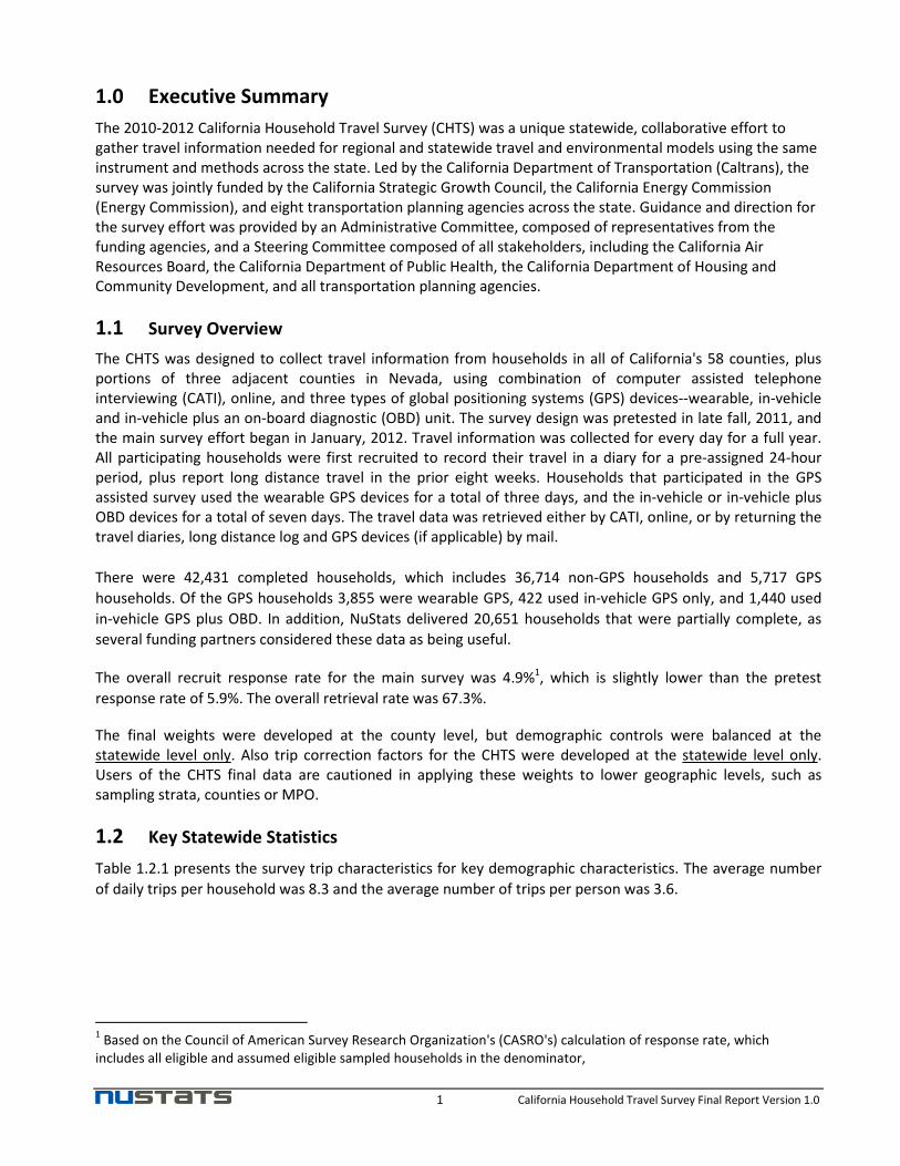
1.0 Executive Summary
The 2010-2012 California Household Travel Survey (CHTS) was a unique statewide, collaborative effort to
gather travel information needed for regional and statewide travel and environmental models using the same
instrument and methods across the state. Led by the California Department of Transportation (Caltrans), the
survey was jointly funded by the California Strategic Growth Council, the California Energy Commission
(Energy Commission), and eight transportation planning agencies across the state. Guidance and direction for
the survey effort was provided by an Administrative Committee, composed of representatives from the
funding agencies, and a Steering Committee composed of all stakeholders, including the California Air
Resources Board, the California Department of Public Health, the California Department of Housing and
Community Development, and all transportation planning agencies.
1.1 Survey Overview
The CHTS was designed to collect travel information from households in all of California's 58 counties, plus
portions of three adjacent counties in Nevada, using combination of computer assisted telephone
interviewing (CATI), online, and three types of global positioning systems (GPS) devices--wearable, in-vehicle
and in-vehicle plus an on-board diagnostic (OBD) unit. The survey design was pretested in late fall, 2011, and
the main survey effort began in January, 2012. Travel information was collected for every day for a full year.
All participating households were first recruited to record their travel in a diary for a pre-assigned 24-hour
period, plus report long distance travel in the prior eight weeks. Households that participated in the GPS
assisted survey used the wearable GPS devices for a total of three days, and the in-vehicle or in-vehicle plus
OBD devices for a total of seven days. The travel data was retrieved either by CATI, online, or by returning the
travel diaries, long distance log and GPS devices (if applicable) by mail.
There were 42,431 completed households, which includes 36,714 non-GPS households and 5,717 GPS
households. Of the GPS households 3,855 were wearable GPS, 422 used in-vehicle GPS only, and 1,440 used
in-vehicle GPS plus OBD. In addition, NuStats delivered 20,651 households that were partially complete, as
several funding partners considered these data as being useful.
The overall recruit response rate for the main survey was 4.9%1, which is slightly lower than the pretest
response rate of 5.9%. The overall retrieval rate was 67.3%.
The final weights were developed at the county level, but demographic controls were balanced at the
statewide level only. Also trip correction factors for the CHTS were developed at the statewide level only.
Users of the CHTS final data are cautioned in applying these weights to lower geographic levels, such as
sampling strata, counties or MPO.
1.2 Key Statewide Statistics
Table 1.2.1 presents the survey trip characteristics for key demographic characteristics. The average number
of daily trips per household was 8.3 and the average number of trips per person was 3.6.
1 Based on the Council of American Survey Research Organization's (CASRO's) calculation of response rate, which
includes all eligible and assumed eligible sampled households in the denominator,

2 California Household Travel Survey Final Report Version 1.0
Table 1.2.1: 2010-2012 CHTS Average Trip Rates by Demographic Characteristic (Weighted)
Item Trips per household/person per day
Household 9.2
Person 3.6
Household size
1 3.3
2 5.7
3 9.7
4+ 17.3
Household vehicles
0 7.5
1 7.3
2 11.5
3+ 9.3
Household employee
0 4.8
1+ 10.6
Income Level
Less than $10,000 8.8
$10,000 to $24,999 8.6
$25,000 to $34,999 8.6
$35,000 to $49,999 8.6
$50,000 to $74,999 8.6
$75,000 to $99,999 9.6
$100,000 to $149,999 10.5
$150,000 to $199,999 11.1
$200,000 to $249,999 10.9
$250,000 or more 10.8
Gender
Male 3.4
Female 3.7
Age
Less than 20 years 3.3

3 California Household Travel Survey Final Report Version 1.0
Item Trips per household/person per day
20 - 24 years 3.2
25-34 years 3.7
35 - 54 years 4.3
55 - 64 years 3.7
65 years or older 2.9
Hispanic Status
Yes 3.5
No 3.6
Employment Status
Yes 4.0
No 3.2
Driver License
Yes 3.8
No 3.1
Table 1.2.2 presents summary trip statistics, including average travel time for trips. Total trips include all
household trips by all modes of travel. Auto trips include driver/passenger trips of household vehicles,
carpool/vanpool, motorcycle, and rental car trips. Driver trips include household vehicle driver trips. Included
in transit trips are private shuttle, greyhound bus, local bus, rapid bus, express bus, commuter bus, premium
bus, public transit shuttle, Dial-a-Ride/paratransit, Amtrak Bus, Other bus, Bart, Metro lines, ACE, Amtrak,
Caltrans, Metro lines, and MUNI.
Table 1.2.2: Key 2010-2012 California Household Travel Survey Trip Statistics (Weighted and expanded)
Weekdays Weekend Total
Total Household Trips1 101,107,350 31,211,141 132,318,491
Total Household Auto Trips2 76,390,785 25,406,487 101,797,272
Total Household Driver Trips3 51,438,843 14,168,011 65,606,854
Total Transit Trips4 4,643,281 1,070,130 5,713,411
Avg. Daily Household Trips (Per Person) 9.8 7.7 9.2
Avg. Daily Person Trips (Per Person) 3.8 3.0 3.6
Avg. Daily Driver Trips Per Household 5.0 3.5 4.6
Avg. Daily Transit Trip per Household 0.5 0.3 0.4
Avg. Trip Length (All Trips in U.S. In minutes) 17.1 19.6 17.7
Avg. Trip Length (Home to Work Trips5) 26.0 23.9 25.8 1Total trips include all household trips by all modes of travel.
2Auto trips include driver/passenger trips of household vehicles, carpool/vanpool, motorcycle, rental car.
3Driver trips include household vehicle driver trips.
4Transit trips include private shuttle, greyhound bus, local bus, rapid bus, express bus, commuter bus, premium bus, public transit shuttle, Dial-a-
Ride/paratransit, Amtrak Bus, Other bus, Bart, Metro lines, ACE, Amtrak, Caltrans, Metro lines, MUNI. 5Home to Work Trips include unlinked trips between home and work place.

4 California Household Travel Survey Final Report Version 1.0
Comparing the 2010-2012 CHTS with the 2000 CHTS, the most frequent mode of travel continued to be auto
driver (49.3% of all reported trips) followed by auto passenger (25.9%). However, the 2010-2012 survey
showed an increased share of walk trips (16.6%), public transportation trips (4.4%), and bicycle trips (1.5%), as
may be seen in Table 1.2.3.
Table 1.2.3: Comparison of 2010-2012 and 2000 CHTS Travel Mode Distribution
Mode
2010-2012
Mode Share
2000 Mode
Share
Auto/Van/Truck Driver 49.3% 60.2%
Auto/Van/Truck Passenger 25.9% 25.8%
Walk Trips 16.6% 8.4%
Public Transportation Trips 4.4% 2.2%
Bicycle Trips 1.5% 0.8%
Private Transportation Trips 0.6%
School Bus Trips 0.6%
Carpool/Vanpool 0.6%
All Other 0.5% 0.7%
Total 100.0% 100.0%
The key trip statistics are presented in Table 1.2.4.
Table 1.2.4: Key Trip Statistics (Unlinked Trips)
Key Trip Statistics
Average household trip 9.2
Average person trip 3.6
% zero trip household 14%
% auto trips 76.9%
% transit trips 4%
Average trip duration (minutes) 17.7
Average work trip duration (minutes) 21.3
Average school trip duration (minutes) 14.6
Average travel distance (route distance in miles) 6.8

5 California Household Travel Survey Final Report Version 1.0
2.0 Introduction
2.1 Survey Objectives and Overall Approach
The 2010 - 2012 California Household Travel Survey (CHTS) was a multi-modal study of the demographic and
travel behavior characteristics of residents across the entire State of California, and the largest single regional
household travel survey ever conducted in the United States. Detailed travel behavior information was
obtained from over 42,500 households, using multiple data collection methods, including Computer Assisted
Telephone Interviewing (CATI), Online, Mail surveys, wearable and in-vehicle GPS as well as using On-Board
Diagnostic (OBD) sensors that gathered data directly from a vehicle's engine, which was a new and innovative
approach. Details of personal travel behavior within region of residence, and inter-regionally within the State,
as well as adjoining states and Mexico, were gathered. The survey sampling plan was designed to ensure an
accurate representation of the entire population of the State. Under the leadership of the California
Department of Transportation (Caltrans), the study was jointly sponsored and funded by Caltrans, the
California Strategic Growth Council, the California Energy Commission, and the following local transportation
planning agencies:
• Association of Monterey Bay Area Governments (AMBAG)
• Fresno Council of Governments
• Kern Council of Governments
• Metropolitan Transportation Commission (MTC)
• San Joaquin Air Pollution Control District
• Santa Barbara County Association of Governments
• Southern California Association of Governments (SCAG)
• Tulare County Association of Governments.
Other state agencies, including the California Air Resources Board, California Department of Public Health, and
California Department of Housing and Community Development as well as all of the State’s Metropolitan
Planning Organizations (MPOs) and Regional Transportation Planning Agencies (RTPAs) were survey
stakeholders. The Federal Highway Administration (FHWA) had active involvement with the survey and
assisted Caltrans with funding for a public outreach program.
The main objective of the survey was to be able to apply the data to develop and update transportation
models in order to meet statutory requirements of both Federal (air quality analysis) and State (AB 32, SB 375
and SB 391). Other main objectives included gathering data from a considerably larger sample than in the
past, a robust collection of all travel modes and use of tolled facilities data, proper targeting of long distance
travel, and an accurate representation of weekday and weekend travel. The 2010 - 2012 CHTS included
additional features to support advanced model development, which included more detailed data on vehicle
acquisition decisions, parking choices, work schedules and flexibility, use of toll lanes/priced facilities, and
walk and bicycle trips. Figure 2.1.1 shows a map of the State of California with counties color coded by
MPO/RTPA, which comprised the study area for the CHTS.

6 California Household Travel Survey Final Report Version 1.0
Figure 2.1.1: County and MPO/RTPA Map of the Household Travel Survey Study Area
SRTA

7 California Household Travel Survey Final Report Version 1.0
2.2 Description of the Survey Components
An overview of the three key aspects of the CHTS survey design is presented in Figure 2.2.1. These three
aspects, Sample Type, Household Type, and Survey Mode, are described as follows:
� Sample Type: The sampling frame for the CHTS was an address-based sample. Households whose
addresses were sampled fell into two types—those for which there was a telephone number matched
to the address (Matched Sample) and those without a matching telephone number (Unmatched). In
general, Matched Sample households have landline telephones, and Unmatched Sample households are
those with cell phone numbers only.
� Household Type: Households were recruited as: 1) those using Global Positioning System (GPS) logging
devices (GPS Households) to augment their travel reporting and, 2) those not (Non-GPS). In the CHTS
design, GPS households were further recruited to use one of three different types of GPS devices:
� Wearable GPS only,
� Vehicle GPS only, or
� Vehicle GPS and On-Board Diagnostic (OBD) engine sensors.
� Survey Mode: To provide potential respondents with multiple ways to respond, there were different
survey modes offered in the Recruit and Retrieval phase of the survey. Recruitment was available to all
Household Types through computer-assisted telephone interviewing (CATI) as well as on the Internet
through the CHTS website. Retrieval of travel and activity information was offered through CATI and
Online, as well as by Mail for Non-GPS Households.
Figure 2.2.1 presents the CHTS survey design in schematic format. The tables presented in this report use the
terminology shown in the schematic and defined above for data reporting.
Figure 2.2.1: CHTS Survey Design Schematic
Sample Type Household
Type
Survey Mode
Recruitment Retrieval
CATI Online CATI Online Mail
Matched or Unmatched
Sample
GPS Households
Wearable GPS
Vehicle GPS
GPS & OBD
Non-GPS Households
Traditionally, household travel surveys have two phases—Recruitment, in which households are screened for
participation and Retrieval, in which the detailed travel and activity information is collected. The CHTS
included a larger than typical number of questions in the Recruitment phase, with the addition of more
vehicle specific questions, which included fuel and vehicle types. The Retrieval phase included the collection
of detailed household travel information from all survey respondents, as well as additional information
including:
• Detail from all CHTS respondents about the activities performed at each location, including an
additional series of questions about up to three activities conducted at each location and the number of
persons participating in each activity with the respondent. For respondents in the SCAG region only,

8 California Household Travel Survey Final Report Version 1.0
respondents were also asked to identify the relationship of persons participating with the respondent in
each activity;
• A separate Long Distance Travel Log, which asked about long distance (LD) travel made in the eight
weeks prior to the assigned travel day.
2.3 Survey Oversight Committees
Oversight of the CHTS was provided by two by two large committees; the Administrative Committee (AC) and
the Steering Committee (SC) along with several Technical Advisory Committees (TAC). The full listing of each
committee’s members may be found in Appendix R.
• The AC was comprised of representatives from the Caltrans administration team, representatives of
the sponsoring agencies, consultants and one technical advisor. All major decisions regarding survey
design and methodology were presented to the AC for their review and approval. AC meetings were
held on the second Wednesday of each month. SC meetings were held on the third Wednesday of
each month.
• The SC was comprised of representatives of other survey stakeholders, including the local MPOs,
RTPAs and the California Air Resources Board, in addition to the AC members. The SC received reports
of the survey progress and the AC’s decisions, and provided input into the survey methodology and
deliverables. The SC members held a stake in this highly complex project. Due to the varied interest,
the AC’s oversight played an integral role in ensuring decisions would be agreed upon, executed, and
properly documented.
• The TAC for Hard-to-Reach Populations Subcommittee provided guidance to the contractor tasked
with public outreach targeted toward the hard to reach population groups. Subcommittee meetings
were held monthly from April 2012 through November 2012.
• The TAC for CHTS Long Distance & Inter-regional Trips Subcommittee - This TAC was composed of
Caltrans, NuStats team members, members of the Administrative Committee and technical experts on
long distance data collection and modeling. It was active in early design phase of the CHTS (2010), and
provided guidance in the development of the long distance survey including key decisions such as the
definition of a long distance trip.
• The TAC for OBD Subcommittee - This TAC was composed of the NuStats team with GeoStats, and
representatives of Caltrans, CEC and ARB. It was active during the CHTS design phase (2010) and
focused on the OBD instrument parameters as well as on air quality and fuel type usage questions on
the CHTS main survey.
• The TAC for Data and Model Transferability Subcommittee - This TAC consisted of Caltrans and
members of the Administrative Committee. It was active in the CHTS early design phase (2010) and its
primary purpose was to evaluate the feasibility of model/data transferability for MPOs/RTPAs where
the CHTS alone cannot meet minimum model estimation requirements.
2.4 Survey Schedule
Figure 2.4.1 below shows the schedule by task for the CHTS. The timing of tasks is described below:

9 California Household Travel Survey Final Report Version 1.0
• Tasks 1 (Project Coordination) has been ongoing for the life of the project and will complete with the
final delivery.
• Task 2 (Project Management) has been ongoing for the life of the project will complete with the final
delivery.
• Task 3 (Develop and Finalize Survey Design) encompassed all of the activities for design of the pretest
and full study.
• Task 4 (Conduct Survey Pretest) consisted of all activities involved in conducting recruitment, retrieval
and preparation of the data for the pretest data file.
• Task 5 (Evaluate Survey Pretest Results) included the activities necessary to analyze the pretest data,
and recommend revisions to the survey methods and materials.
• In Task 6 (Refine Survey Methods – for Full Study) activities dedicated to this task included revision of
all survey materials and programs, and the additional efforts to translate all materials and programs
into Spanish. In order to maintain the project schedule, the English survey work began prior to
finalizing the Spanish, which is why the finish date for Task 6 ends after the full study begins.
• Task 7 (Conduct Full Study) begins with the mailing of the first wave of advanced letters, and finishes
at the conclusion of cleaning the data in preparation for building the data file.
• Task 8 (Process and Analyze Data) begins with the first retrieval data, and ends with the finalizing the
analysis.
• Task 9 (Final Reports and Recommendations) will be the final task for this project.
Figure 2.4.1: Survey Schedule

10 California Household Travel Survey Final Report Version 1.0
3.0 Survey Design
The final goal of the CHTS full study, based on the pretest results and special requests from funding partners,
was to collect the following survey samples:
• 53,483 California households, with the number of households sampled proportionate to the
population in the sampling strata;
• Of these, 48,384 households were to be Non-GPS and 5,099 were to be GPS Households
• Of the GPS households, the desired distribution was:
� 400 Wearable devices
� 3,099 MTC Wearable devices
� 400 Vehicle GPS devices
� 800 Vehicle and OBD devices
� 400 Energy Commission Vehicle GPS and OBD devices
3.1 Survey Instrument and Materials Design
The survey instruments for the CHTS were developed collaboratively with Caltrans, NuStats, and GeoStats and
with input from the Steering Committee. The survey instruments were based on steering committee
members’ travel modeling and analytical needs.
The key data elements identified and collected were as follows:
• Household Characteristics – main household characteristics collected were:
a) Physical address, including county of residence
b) Household size
c) Type of residence
d) Home ownership status
e) Number of years at current address and previous address if at current address for less than 6
years
f) Number of cell and landline phone numbers in household
g) Use of public transportation
h) Bicycle availability and number of bicycles available to the household for use
i) Plan to purchase new vehicle in the next five years
j) Vehicle availability and number of vehicles available to the household for use
• Person Characteristics - Demographic information was collected for all household members to help
explain the impact of household dynamics on personal travel in the region. The person-level data
elements were:
a) Name, Gender, Age and Race
b) Relationship among household members
c) Country of birth and year moved to US if not natural born citizen
d) Number in household who possess driver’s license

11 California Household Travel Survey Final Report Version 1.0
e) Employment status, location of employment, and if more than one employer, type of industry
and occupation
f) If disabled type of disability and if hold disabled license plate or disabled transit registration,
eligibility for transit subsidy and amount of subsidy
g) Typical work days, number of hours worked per week, availability of working flexible hours,
and mode of transportation to and from work location, HOV lane availability and use
h) If any household members are of Hispanic, Latino or Spanish origin
i) Student status, grade level, location of school, home or on-line schooled, level of education
completed
• Vehicle Characteristics - The recruitment instrument included questions about the vehicles available
to the household:
a) Year, Make, Model, Series, Body type, Transmission type, Drive/Power Train (FWD, AWD, etc.)
and Number of cylinders
b) Vehicle fuel type (hybrid, gasoline, diesel, etc.)
c) Vehicle new or used when acquired
d) Vehicle owned, borrowed or leased
e) Vehicle covered by Pay-as-You-Drive insurance
f) Vehicle driven on assigned travel day, or if not driven reason not driven
g) Devices provided by insurance company to detect mileage driven
h) For GPS households, information on working power outlet or cigarette lighter socket in
vehicle
i) If electric vehicle, the number of feet to nearest electric outlet and if it is 110 or 220 volt
• Activities – The retrieval interview collected information about each person’s activities throughout
their assigned travel period. These data elements included:
a) Participation in activity/activities alone or with others and the number of others who
participated
b) Activity start time/end time
• Trip Data – During the retrieval interview, trip data was collected for each household member, and
included the following:
a) Number of household members who traveled
b) Trip modes
c) Parking type, cost (and if reimbursed by employer), duration, location, and if household
members remained in the vehicle at stopping point
d) Arrival and departure time
e) Use of transit, if so, which transit system and route
f) Vehicle(s) driven by each household member and if transit passes, tolled facilities or car
sharing were utilized by any member of the household, and if so, the specifics of each
g) Trip place name and address
For the CHTS full study, the following process was utilized:

12 California Household Travel Survey Final Report Version 1.0
• Advanced Mailing - Advanced letters were mailed to households approximately 1 week prior to
placing recruitment calls. The purpose of the advanced letter was to notify households they had been
chosen to be eligible to participate in the CHTS. By sending advanced notification, households had the
chance to read about the study prior to receiving a recruitment telephone call. The advanced letters
contained the Personal Identification Number (PIN) assigned to that specific household. Additionally,
the advanced letter served to inform households of the available option to complete recruitment
online via the CHTS website, or to call the hotline to complete via CATI. Three rounds of advanced
postcards were sent in May and June 2012, however, this method was found to be less effective than
advanced letters and was discontinued. An example of the advanced letter may be found in Appendix
A.
• Recruitment Interview – Generally within one week of sending advanced letters, households would
begin completing recruitment online. Once Online recruitment had begun, the recruitment interview
telephone calls would begin. The recruitment interviews were conducted using CATI and Online and
secured the household to participate in the CHTS. The recruitment introduction was specifically
designed to obtain agreement to participate. The recruitment questionnaire collected all of the key
data elements listed above. The recruitment CATI and online scripts are included in Appendix B and
Appendix C, respectively.
• Respondent Material Mailing – The demographic information collected during recruitment was
utilized to prepare personalized cover letters for the recruited households. The cover letter included
the household’s PIN, the assigned travel day, instructions for completing the diary, and instructions
for completing the long distance log. Additionally, diaries were personalized for each member of the
household. Appendix G contains an example of the materials included in the respondent mailing
packet. Appendix J is an example of the long distance materials. Households participating in the GPS
component of the survey were mailed the appropriate GPS equipment and instructions for the
equipment, along with travel diary packet materials and a long distance log. The GPS travel diary
packet materials may be found in Appendix H. The Energy Commission materials may be found in
Appendix I.
• Reminder Contact – At the time of recruitment, respondents were given the option to receive their
travel reminder via telephone call, email, or text message. The day prior to the assigned travel day (or
two days prior if the day before their travel day was a holiday) each household was contacted via their
requested form of contact, to remind them of their impending travel day, confirm receipt of travel
materials, answer any questions the respondents may have, and provide the hotline number. If the
travel packet was not received by the time of the reminder, respondents were given instructions on
how to download the materials from the survey website. In the case of GPS materials not being
received, the households were given the option to reschedule. Non-GPS households were only given
the option to reschedule under specific circumstances. Scripts for the reminder calls, emails and text
messages may be found in Appendix D.
• Retrieval Interview – Retrieval was completed in one of three modes: CATI, Online and Mail. If
responding households had not logged onto the survey website to complete their retrieval interview
the day following their assigned travel day, retrieval calls were placed to collect the travel data. The
CATI and Online programs were set up to encourage respondents to answer every required question,
and to terminate the retrieval interview if respondents refused. The telephone representatives were
trained on refusal rebuttals to minimize terminations. The CATI program also prompted interviewers
to reference the same trips made by other household members. A look-up table of frequently visited

13 California Household Travel Survey Final Report Version 1.0
locations aided with the retrieval process. The retrieval questionnaire utilized in the CATI interviews is
found in Appendix D. The questionnaire utilized for Online retrieval is found in Appendix E. The non-
GPS travel diary packet materials may be found in Appendix G. Appendix H contains the GPS travel
diary packet materials.
3.2 Sample Design
3.2.1 Source of Sample and Survey Universe
An Address-based sampling frame approach was used. An Address-based sample is a random sample of all
residential addresses that receive U.S. Mail delivery. Its main advantage is its reach into population groups
that typically participate at lower-than-average levels, largely due to coverage bias (such as households with
no phones or cell-phone only households). For efficiency of data collection, NuStats matched addresses to
telephone numbers that had a listed name of the household appended to the sampled mailing addresses. This
sampling frame ensured coverage of all types of households irrespective of their telephone ownership status,
including households with no telephones (estimated at less than 3% of households in the U.S.).
In order to better target the hard-to-reach groups, the address-based sample were supplemented with
samples drawn from the listed residential frame that included listed telephone numbers from working blocks
of numbers in the United States for which the name and address associated with the telephone number were
known. The “targeted” Listed Residential sample, as available from the sampling vendor, included low-income
listed sample, large-household listed sample, young population sample, and Spanish-surname sample (to
name a few). As expected, this sample was used to further strengthen the coverage of hard-to-reach
households. The advantage of drawing sample from this frame is its efficiency in conducting the survey
effort—being able to directly reach the hard-to-reach households and secure their participation in the survey
in a direct and active approach. Both address and listed residential samples were procured from the sample
provider – Marketing Systems Group (MSG) based in Fort Washington, PA.
The survey population was representative of all households residing in the 58 counties in California. According
to 2010 Census data, the survey universe comprised 12,577,498 households. Table 3.2.3.1 provides the
distribution of households by counties and by MPO/RTPA. As shown in the table, 83% resided in four MPO
regions (spread over 22 counties) – 46% in SCAG, 21% in MTC, 9% in SANDAG, and 7% in SACOG. The
remaining 17% households reside in 36 counties in California
3.2.2 Sampling Design and Selection Methodology
NuStats employed a stratified probability sample of households for the CHTS 2010-2012 Full Study. Stratified
sampling is a type of random or probability sampling, the methods of which are well grounded in statistical
theory and the theory of probability. Specifically, stratified sampling is a probability sampling method where
the survey universe is divided into smaller groups and a random sample is chosen within each group (i.e.,
every sampling unit has some non-zero probability of being selected into the sample). This method resulted in
over-sampling for some strata ensuring NuStats captured the diversity of the population according to specific
factors affecting travel behavior in the study area. Thus, within strata, households were selected with equal
probabilities but the combined sample (across strata) comprised an unequal probability sample of
households.
To ensure geographic representation, NuStats utilized a geographic stratification scheme, which ensured
adequate representation of households throughout the study area. A stratified random sample that was
disproportionate to the distribution of households by county of residence was drawn.

14 California Household Travel Survey Final Report Version 1.0
The study area had a high concentration of hard-to-reach groups (see Tables 3.2.3.4 through 3.2.3.7 pages 23-
27):
• 31% large households (i.e., 4 or more member households)
• 22% low-income households (i.e., households with annual income less than $25,000)
• 36% younger population (i.e., 25 years of age or less)
• 38% Hispanic population
• 8% zero-vehicle households.
As a result, NuStats implemented a selective oversampling strategy. Specifically, the oversampling strategy
was two-fold: (1) oversample addresses from the census tracts with high concentrations of hard-to-reach
groups, and (2) supplement the address-based samples with ‘targeted’ listed residential samples. Besides
utilizing sampling-based methods, NuStats also utilized intercept-based surveying methods to recruit transit-
using households for Kern County2. Based on Hispanic household, person age, household size data from the
Census 2010 by census tract, and household income and number of household vehicle data from the
American Community Survey (ACS), a five year estimate for 2005-09 which were the latest available
reference data during the sampling design stage, NuStats identified census tracts with a high concentration of
these hard to reach households.
As shown in the Figures 3.2.3.2 through 3.2.3.6, the census tracts were classified into four segments based on
a weighted quartile distribution of hard-to-reach segments (weighted by the hard-to-reach segment counts),
where each quartile included 25% of hard-to-reach segment counts. To illustrate, the top quartile in the
Hispanic population distribution denoted as “Greater than 77%” in Figure 3.2.3.2 included all census tracts
with more than 77% Hispanic residents at the census tract level (as identified by the 75th percentile) and
represented 3,506,974 Hispanic residents that made up 25% of the Hispanic population. NuStats oversampled
the hard-to-reach population segments from the “top two” quartiles with higher rate of oversampling from
the topmost quartile. It is important to note that the figures presented in this section used the weighted
quartile distribution to the segment count and therefore, do not directly represent a sample distribution of
each target population group to the total population from 2010 Census data. The oversampling rates were
adjusted across sample orders by MPOs/RTPAs depending on the incidence of completed surveys from hard-
to-reach groups.
NuStats also supplemented this effort with listed samples available from our vendor for hard-to-reach groups.
This included low-income listed sample, large-household listed sample, young household headed listed
sample and Hispanic surname sample (to name a few). In addition to the aforementioned hard-to-reach
groups, NuStats also oversampled transit-using households and zero vehicle households to ensure there was
adequate representation of the travel patterns of transit users. Specifically, NuStats oversampled all
households residing within 0.25 mile of the transit lines or bus stops, and 0.5 mile of the rail stations (see
Figure 3.2.3.7, page 22).
Note that the geographic and socioeconomic stratifications were monitored separately. In addition, the
sample performance was closely monitored to ensure that adequate representation of hard-to-reach
demographic groups was realized. In cases of under-representation, the specifications of the subsequent
2 This effort was funded by Kern County.

15 California Household Travel Survey Final Report Version 1.0
sample orders were adjusted to oversample these demographic groups. Subsequent sample orders were
adjusted based on the following evaluation criteria:
• What was the response rate? Were as many surveys completed as expected with the amount of
sample ordered?
• How much of the sample was eligible vs. ineligible?
• For the completed surveys, what were the demographic distributions of each sample type
compared to the Census distributions? Did the targeted listed residential sample successfully find
the hard-to-reach population groups?
• Was the progress towards the geographic and demographic stratifications goals consistent, or
were some geographic/demographic segments not performing as well as others?
3.2.3 Geographic Distribution
Figure 3.2.3.1 is a map showing the thirty sampling strata in the study area and were utilized to manage the
recruitment and retrieval goals for the CHTS. A sampling structure was developed to oversample under
represented areas, resulting in a distribution considered by the AC to be statistically accurate at the county
level. The first 2/3 of the total sample size of households was allocated based on a proportional distribution of
the number of households within each county relative to the entire state. The remaining 1/3 of household
samples were targeted towards the “rural” counties, which included all counties except the top ten counties
with the largest number of households. Table 3.2.3.1 delineates the distribution of households that comprised
the study area.

16 California Household Travel Survey Final Report Version 1.0
Figure 3.2.3.1: A map of 30 sampling strata (see pages 19-20 for counties included in each strata)

17 California Household Travel Survey Final Report Version 1.0
Table 3.2.3.1: Distribution of Sampled Households in the Study Area
MPO/RTPA County
Total
Households
Percent of Total
Households
Total
Households
Percent of Total
Households
SCAG
Los Angeles 3,241,204 26%
5,847,909 46%
Orange 992,781 8%
Riverside 686,260 5%
San Bernardino 611,618 5%
Ventura 266,920 2%
Imperial 49,126 <1%
MTC
Santa Clara 604,204 5%
2,608,023 21%
Alameda 545,138 4%
Contra Costa 375,364 3%
San Francisco 345,811 3%
San Mateo 257,837 2%
Sonoma 185,825 1%
Solano 141,758 1%
Marin 103,210 1%
Napa 48,876 <1%
SANDAG San Diego 1,086,865 9% 1,086,865 9%
SACOG
Sacramento 513,945 4%
826,067 7%
Placer 128,160 1%
Yolo 70,872 1%
El Dorado 57,346 <1%
Sutter 31,437 <1%
Yuba 24,307 <1%
Fresno Fresno 289,391 2% 289,391 2%
Kern Kern 254,610 2% 254,610 2%
AMBAG
Monterey 125,946 1%
237,106 2%
Santa Cruz 94,355 1%
San Benito 16,805 <1%
San Joaquin San Joaquin 215,007 2% 215,007 2%
Stanislaus Stanislaus 165,180 1% 165,180 1%
Santa Barbara Santa Barbara 142,104 1% 142,104 1%
Tulare Tulare 130,352 1% 130,352 1%
San Luis Obispo San Luis Obispo 102,016 1% 102,016 1%
Butte Butte 87,618 1% 87,618 1%
Merced Merced 75,642 1% 75,642 1%
Shasta Shasta 70,346 1% 70,346 1%
Humboldt Humboldt 56,031 <1% 56,031 <1%
Madera Madera 43,317 <1% 43,317 <1%
Nevada Nevada 41,527 <1% 41,527 <1%
Kings Kings 41,233 <1% 41,233 <1%

18 California Household Travel Survey Final Report Version 1.0
MPO/RTPA County
Total
Households
Percent of Total
Households
Total
Households
Percent of Total
Households
Mendocino Mendocino 34,945 <1% 34,945 <1%
Lake Lake 26,548 <1% 26,548 <1%
Tehama Tehama 23,767 <1% 23,767 <1%
Tuolumne. Tuolumne 22,156 <1% 22,156 <1%
Siskiyou Siskiyou 19,505 <1% 19,505 <1%
Calaveras Calaveras 18,886 <1% 18,886 <1%
TMPO
El Dorado 12,877 <1%
17,344 <1% Placer 4,467 <1%
Amador Amador 14,569 <1% 14,569 <1%
Lassen Lassen 10,058 <1% 10,058 <1%
Del Norte Del Norte 9,907 <1% 9,907 <1%
Glenn Glenn 9,800 <1% 9,800 <1%
Plumas Plumas 8,977 <1% 8,977 <1%
Inyo Inyo 8,049 <1% 8,049 <1%
Mariposa Mariposa 7,693 <1% 7,693 <1%
Colusa Colusa 7,056 <1% 7,056 <1%
Trinity Trinity 6,083 <1% 6,083 <1%
Mono Mono 5,768 <1% 5,768 <1%
Modoc Modoc 4,064 <1% 4,064 <1%
Sierra Sierra 1,482 <1% 1,482 <1%
Alpine Alpine 497 <1% 497 <1%
12,577,498 100% 12,577,498 100%
The sampling plan was revised on several occasions and was finalized in June 2012, although at the request of
the Administrative Committee (November 14, 2012), the goals were modified to reflect the expected true
goals. In Table 3.2.3.2 and Figure 3.2.3.2, an overall summary of the rebaselined sampling plans through June
2012 is presented. Table 3.2.3.3 presents the rebaselined sample distribution by the 30 sampling strata, with
the modified expected goals.
Table 3.2.3.2: Summary of Sample Plans
SOURCE
NuStats
GRAND TOTAL CHTS
SCAG, Energy
Commission and MPO
Augment
NuStats Total
Non-
GPS GPS Total
Non-
GPS GPS Total
Non-
GPS GPS Total
Non-
GPS GPS Total
Original Proposal (“up to 60,000)
55,000 5,000 60,000 - - - 55,000 5,000 60,000 55,000 5,000 60,000
Sample Plan July
2011 35,695 3,152 37,847 19,514 - 19,514 54,209 3,152 57,361 54,209 3,152 57,361
Sample Plan December 2011
29,443 2,400 31,843 12,234 3,500 15,734 41,677 5,900 47,577 46,377 5,900 52,277
Final Sample Plan
June 2012 36,368 1,600 37,968 12,016 3,499 15,515 48,384 5,099 53,483 37,660 5,099 42,759
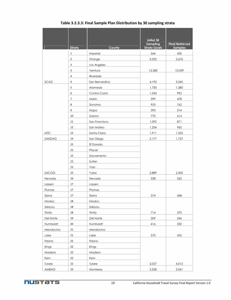
19 California Household Travel Survey Final Report Version 1.0
Table 3.2.3.3: Final Sample Plan Distribution by 30 sampling strata
Strata County
Initial 30
Sampling
Strata Goals
Final Retrieved
Samples
SCAG
1 Imperial 564 450
2 Orange 3,353 2,676
3 Los Angeles
12,580 10,039 3 Ventura
4 Riverside
4,192 3,345 4 San Bernardino
MTC
5 Alameda 1,730 1,380
6 Contra Costa 1,243 992
7 Marin 599 478
8 Sonoma 955 762
9 Napa 393 314
10 Solano 770 614
11 San Francisco 1,092 871
12 San Mateo 1,204 960
13 Santa Clara 1,911 1,525
SANDAG 14 San Diego 2,177 1,737
SACOG
15 El Dorado
2,889 2,305
15 Placer
15 Sacramento
15 Sutter
15 Yolo
15 Yuba
Nevada 16 Nevada 328 262
Lassen 17 Lassen
574 458
Plumas 17 Plumas
Sierra 17 Sierra
Modoc 18 Modoc
714 570
Siskiyou 18 Siskiyou
Trinity 18 Trinity
Del Norte 19 Del Norte 309 246
Humboldt 20 Humboldt 416 332
Mendocino 21 Mendocino
570 455 Lake 21 Lake
Fresno 22 Fresno
5,027 4,012
Kings 22 Kings
Madera 22 Madera
Kern 22 Kern
Tulare 22 Tulare
AMBAG 23 Monterey 2,558 2,041
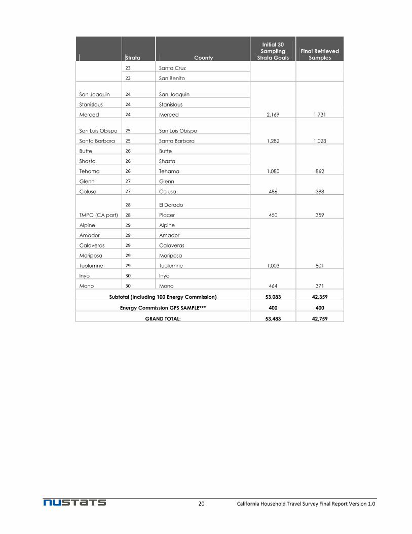
20 California Household Travel Survey Final Report Version 1.0
Strata County
Initial 30
Sampling
Strata Goals
Final Retrieved
Samples
23 Santa Cruz
23 San Benito
San Joaquin 24 San Joaquin
2,169 1,731
Stanislaus 24 Stanislaus
Merced 24 Merced
San Luis Obispo 25 San Luis Obispo
1,282 1,023 Santa Barbara 25 Santa Barbara
Butte 26 Butte
1,080 862
Shasta 26 Shasta
Tehama 26 Tehama
Glenn 27 Glenn
486 388 Colusa 27 Colusa
TMPO (CA part)
28 El Dorado
450 359 28 Placer
Alpine 29 Alpine
1,003 801
Amador 29 Amador
Calaveras 29 Calaveras
Mariposa 29 Mariposa
Tuolumne 29 Tuolumne
Inyo 30 Inyo
464 371 Mono 30 Mono
Subtotal (Including 100 Energy Commission) 53,083 42,359
Energy Commission GPS SAMPLE*** 400 400
GRAND TOTAL: 53,483 42,759

21 California Household Travel Survey Final Report Version 1.0
Figure 3.2.3.2 shows the overall recruitment and retrieval completes throughout the entire duration of the
project. The chart is color coded to present the breakdown of CATI, Online and Mailback recruited and
retrieved completed households. The red line indicates project expenses.
Figure 3.2.3.2 Recruitment and Retrieval Completes Over the Entire Duration
Figure 3.2.3.3 shows the density of the numbers of retrieved samples by strata ranging from 0.6%-25%. The
ranges are color coded as is shown by the key at the lower right corner of the figure.
Recruitment and Retrieval Completes
10/1/10 6/1/11 10/1/12 6/1/12 2/1/12

22 California Household Travel Survey Final Report Version 1.0
Figure 3.2.3.3: Density of Number of Samples by Strata

23 California Household Travel Survey Final Report Version 1.0
Figure 3.2.3.4: Quartile Distribution of Hispanic Population

24 California Household Travel Survey Final Report Version 1.0
Figure 3.2.3.5: Quartile Distribution of Low Income Households (annual income less than $25,000)

25 California Household Travel Survey Final Report Version 1.0
Figure 3.2.3.6: Quartile Distribution of Young Population (25 years of age or less)

26 California Household Travel Survey Final Report Version 1.0
Figure 3.2.3.7: Quartile Distribution of Zero Vehicle Households
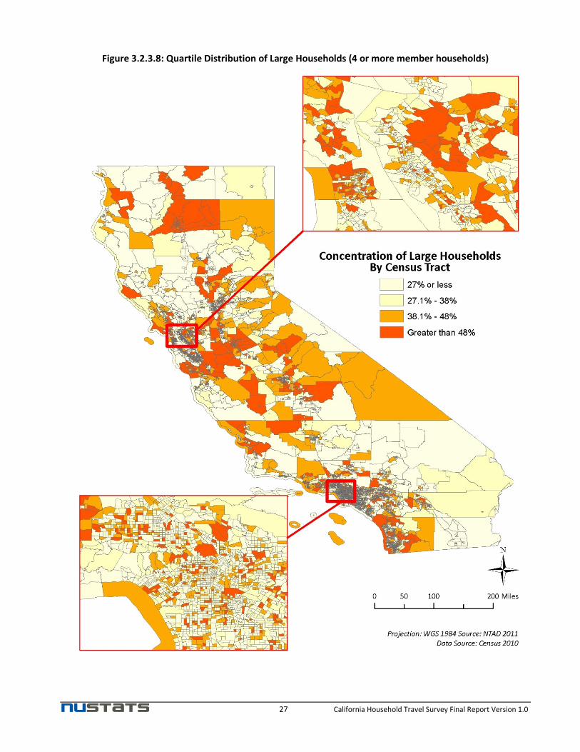
27 California Household Travel Survey Final Report Version 1.0
Figure 3.2.3.8: Quartile Distribution of Large Households (4 or more member households)

28 California Household Travel Survey Final Report Version 1.0
Figure 3.2.3.9: Transit Oversampling Area

29 California Household Travel Survey Final Report Version 1.0
NuStats also used a socioeconomic stratification to set demographic goals. Several demographic
characteristics, including household size, household workers, household vehicles, household income, Hispanic
status, and age of the residents in the study area were monitored. Table 3.2.3.4 provides the 2010 ACS/2010
Census distributions of these key data elements for the overall study area that were tracked in the weekly
reports. The observed socioeconomic distribution of the completed surveys was monitored and compared
with the 2010 ACS data and/or the 2010 Census distributions, to track the extent to which they fell within the
expected ranges.
Table 3.2.3.4: Socio-Demographic Distribution for the Study Area
Total Counts % Counts
Household Size
(Census 2010)
1 2,929,442 23.3%
2 3,653,802 29.1%
3 2,043,812 16.2%
4 or more 3950442 31.4%
Total 12,577,498 100.0%
Household Vehicle
Ownership
(ACS 2010 1 year)
0 969,100 7.8%
1 3,992,884 32.2%
2 4,644,854 37.4%
3 or more 2,799,637 22.6%
Total 12,406,475 100.0%
Household Workers
(ACS 2010 1 year)
0 3,105,348 25.0%
1 4,924,635 39.7%
2 3,388,872 27.3%
3 or more 987,620 8.0%
Total 12,406,475 100.0%
Household Income
(ACS 2010 1 year)
<$25K 2,669,373 21.5%
$25K-$50K 2,770,966 22.3%
$50k-$75K 2,168,573 17.5%
$75K-$100K 1,530,962 12.3%
$100K+ 3,266,601 26.3%
Total 12,406,475 100.0%
Hispanic Status of Residents
(Census 2010)
Hispanic 14,013,719 37.6%
Non-Hispanic 23,240,237 62.4%
Total 37253956 100.0%
Age of Residents
(Census 2010)
<25 yrs 13,217,991 35.5%
25 – 34 yrs 5,317,877 14.3%
35 – 44 yrs 5,182,710 13.9%
45 – 54 yrs 5,252,371 14.1%
55 – 64 yrs 4,036,493 10.8%
65+ yrs 4,246,514 11.4%
Total 37,253,956 100.0%

30 California Household Travel Survey Final Report Version 1.0
4.0 Survey Methods
This section describes the main survey methods. Following a brief discussion of the changes made to the main
survey as a result of the CHTS pretest, the final survey design is presented in detail. Discussions of the following
specific aspects of the survey methods are then presented: proxy reporting, call backs, refusals, hotline, handling
non-English speaking households, interviewer training, incentives, definition of a completed household, long
distance logs, respondent burden, and sample management. Survey outreach to hard to reach populations and
ongoing quality control complete the survey methods.
4.1 Survey Pretest
The CHTS was a unique collaborative effort between several state agencies and all of California's Regional MPOs
and RTPAs, each with varying data needs and desires. While the CHTS was always planned to include many data
elements that were standard items in most travel behavior surveys, there were also many new data items that
the various partner agencies and entities brought forward to be developed and tested in the CHTS pretest.
Accordingly, the pretest was a complete test of all survey items and methods, with specific focus on interview
length.
The CHTS pretest was conducted between August and mid-October, 2011, in English only. There were 1,568
completed households, comprising 1,357 non-GPS households and 211 GPS households (39 wearable GPS, 125
in-vehicle GPS, and 47 in-vehicle GPS and OBD households). Given the large number of questions tested, it was
not surprising that the CATI interview length for both the recruitment and retrieval interviews was longer than
estimated in the survey budget (22.4 minutes for recruitment as compared to 19 minutes estimated; 23.4
minutes for retrieval compared to 21 minutes estimated). To reduce the main survey length, the Pretest Peer
Review Panel (a subset of the Administrative and Steering Committee members) approved the following
recommendations:
• Remove items from the main survey that did not compromise the data necessary for modeling;
• Reduce the number of instances some questions were asked by asking them only once during the travel
day instead of for each trip (e.g. use of toll roads);
• Expand the listed response options to reduce the need for "Other, specify" (i.e. open-ended questions).
• Move generic questions from the end of the retrieval interview to the end of the recruitment interview.
• Use targeted sampling to improve the response of under-represented populations; and,
• Enhance the survey instructions and explanations to encourage participation.
4.2 Final Survey Design
The CHTS pretest yielded many recommended revisions to the recruitment and retrieval instruments, and the
changes based on the pretest were implemented in the main survey without the benefit of a second pilot test. As
is discussed in the Limitations section, this meant that some changes may not have yielded the anticipated
benefits. In addition, during the 12 months of main survey data collection, there were changes made to increase
recruitment and retrieval rates for particular populations, to encourage online responses, and to generally raise
the overall level of response. This section presents the final survey design and documents, to the extent possible,
changes made.
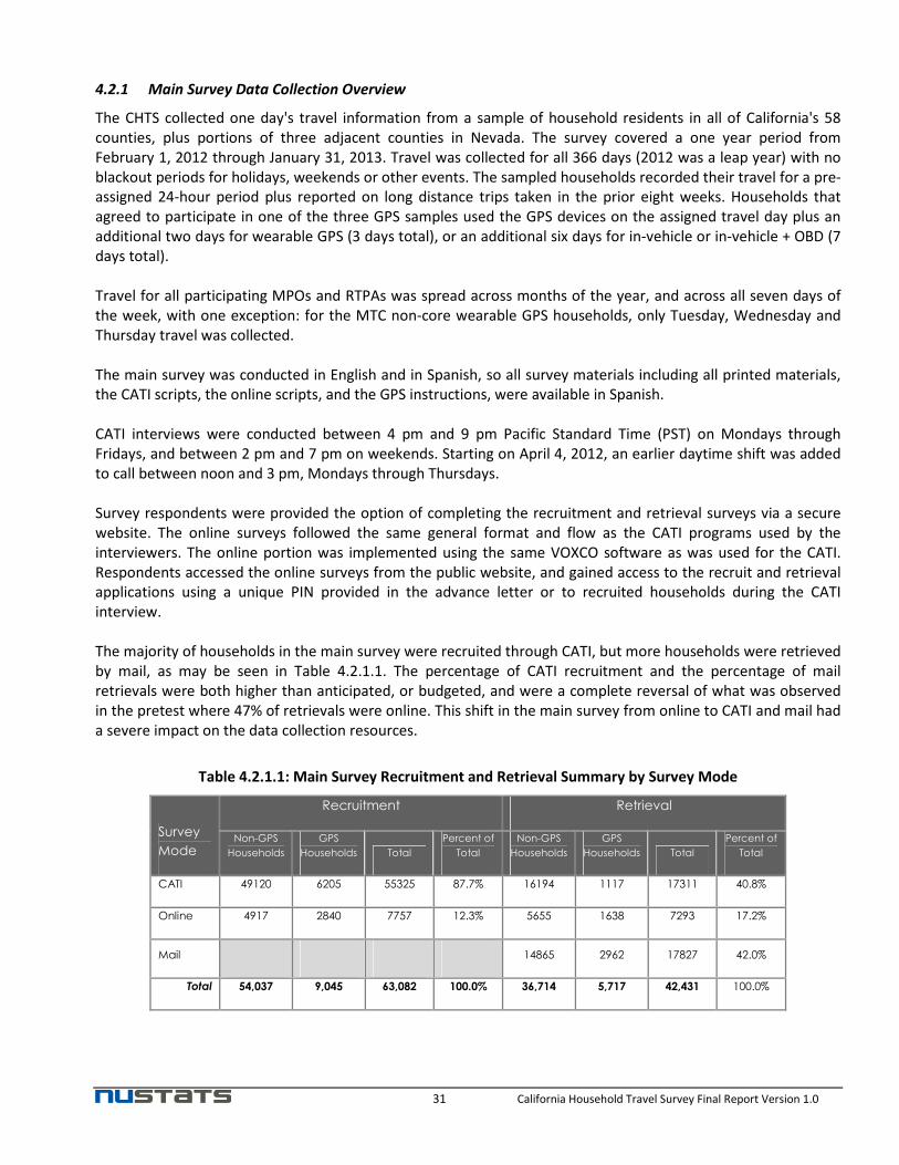
31 California Household Travel Survey Final Report Version 1.0
4.2.1 Main Survey Data Collection Overview
The CHTS collected one day's travel information from a sample of household residents in all of California's 58
counties, plus portions of three adjacent counties in Nevada. The survey covered a one year period from
February 1, 2012 through January 31, 2013. Travel was collected for all 366 days (2012 was a leap year) with no
blackout periods for holidays, weekends or other events. The sampled households recorded their travel for a pre-
assigned 24-hour period plus reported on long distance trips taken in the prior eight weeks. Households that
agreed to participate in one of the three GPS samples used the GPS devices on the assigned travel day plus an
additional two days for wearable GPS (3 days total), or an additional six days for in-vehicle or in-vehicle + OBD (7
days total).
Travel for all participating MPOs and RTPAs was spread across months of the year, and across all seven days of
the week, with one exception: for the MTC non-core wearable GPS households, only Tuesday, Wednesday and
Thursday travel was collected.
The main survey was conducted in English and in Spanish, so all survey materials including all printed materials,
the CATI scripts, the online scripts, and the GPS instructions, were available in Spanish.
CATI interviews were conducted between 4 pm and 9 pm Pacific Standard Time (PST) on Mondays through
Fridays, and between 2 pm and 7 pm on weekends. Starting on April 4, 2012, an earlier daytime shift was added
to call between noon and 3 pm, Mondays through Thursdays.
Survey respondents were provided the option of completing the recruitment and retrieval surveys via a secure
website. The online surveys followed the same general format and flow as the CATI programs used by the
interviewers. The online portion was implemented using the same VOXCO software as was used for the CATI.
Respondents accessed the online surveys from the public website, and gained access to the recruit and retrieval
applications using a unique PIN provided in the advance letter or to recruited households during the CATI
interview.
The majority of households in the main survey were recruited through CATI, but more households were retrieved
by mail, as may be seen in Table 4.2.1.1. The percentage of CATI recruitment and the percentage of mail
retrievals were both higher than anticipated, or budgeted, and were a complete reversal of what was observed
in the pretest where 47% of retrievals were online. This shift in the main survey from online to CATI and mail had
a severe impact on the data collection resources.
Table 4.2.1.1: Main Survey Recruitment and Retrieval Summary by Survey Mode
Survey
Mode
Recruitment Retrieval
Non-GPS
Households
GPS
Households Total
Percent of
Total
Non-GPS
Households
GPS
Households Total
Percent of
Total
CATI 49120 6205 55325 87.7% 16194 1117 17311 40.8%
Online 4917 2840 7757 12.3% 5655 1638 7293 17.2%
Mail 14865 2962 17827 42.0%
Total 54,037 9,045 63,082 100.0% 36,714 5,717 42,431 100.0%

32 California Household Travel Survey Final Report Version 1.0
4.2.2 Survey Processes
The main survey followed the traditional two-step process of recruitment of a household for a prospective
assigned travel day, followed by a separate retrieval effort to collect the detailed travel information. Figure
4.2.2.1 shows the survey process utilized for the CHTS main survey.
Figure 4.2.2.1: CHTS Survey Process
The sequential survey processes discussed below include:
• Advance Letters
• Recruitment
• Survey Materials
• Reminder Contact
• Retrieval
Advance Letters
Advance letters provided potential participants with basic information about the survey, and were initially mailed
to all sampled households in December, 2011 when recruitment started. Subsequent analyses of the
effectiveness of the advance letters indicated they were less effective among matched households. This led to a
change in the protocol in February 2012 so that advance letters were only sent to:
• All unmatched households;
• All households in the GPS samples, regardless of type of GPS; and,
• All households that were in any of the targeted samples, regardless of whether they were matched or
unmatched households
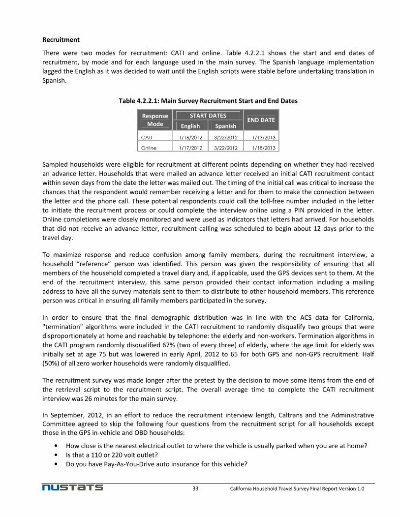
33 California Household Travel Survey Final Report Version 1.0
Recruitment
There were two modes for recruitment: CATI and online. Table 4.2.2.1 shows the start and end dates of
recruitment, by mode and for each language used in the main survey. The Spanish language implementation
lagged the English as it was decided to wait until the English scripts were stable before undertaking translation in
Spanish.
Table 4.2.2.1: Main Survey Recruitment Start and End Dates
Response
Mode
START DATES END DATE
English Spanish
CATI 1/16/2012 3/22/2012 1/13/2013
Online 1/17/2012 3/22/2012 1/18/2013
Sampled households were eligible for recruitment at different points depending on whether they had received
an advance letter. Households that were mailed an advance letter received an initial CATI recruitment contact
within seven days from the date the letter was mailed out. The timing of the initial call was critical to increase the
chances that the respondent would remember receiving a letter and for them to make the connection between
the letter and the phone call. These potential respondents could call the toll-free number included in the letter
to initiate the recruitment process or could complete the interview online using a PIN provided in the letter.
Online completions were closely monitored and were used as indicators that letters had arrived. For households
that did not receive an advance letter, recruitment calling was scheduled to begin about 12 days prior to the
travel day.
To maximize response and reduce confusion among family members, during the recruitment interview, a
household “reference” person was identified. This person was given the responsibility of ensuring that all
members of the household completed a travel diary and, if applicable, used the GPS devices sent to them. At the
end of the recruitment interview, this same person provided their contact information including a mailing
address to have all the survey materials sent to them to distribute to other household members. This reference
person was critical in ensuring all family members participated in the survey.
In order to ensure that the final demographic distribution was in line with the ACS data for California,
"termination" algorithms were included in the CATI recruitment to randomly disqualify two groups that were
disproportionately at home and reachable by telephone: the elderly and non-workers. Termination algorithms in
the CATI program randomly disqualified 67% (two of every three) of elderly, where the age limit for elderly was
initially set at age 75 but was lowered in early April, 2012 to 65 for both GPS and non-GPS recruitment. Half
(50%) of all zero worker households were randomly disqualified.
The recruitment survey was made longer after the pretest by the decision to move some items from the end of
the retrieval script to the recruitment script. The overall average time to complete the CATI recruitment
interview was 26 minutes for the main survey.
In September, 2012, in an effort to reduce the recruitment interview length, Caltrans and the Administrative
Committee agreed to skip the following four questions from the recruitment script for all households except
those in the GPS in-vehicle and OBD households:
• How close is the nearest electrical outlet to where the vehicle is usually parked when you are at home?
• Is that a 110 or 220 volt outlet?
• Do you have Pay-As-You-Drive auto insurance for this vehicle?

34 California Household Travel Survey Final Report Version 1.0
• Does this vehicle have any devices provided by your insurance company to detect mileage driven?
This change was implemented in mid-September, 2012.
Survey Materials
Following recruitment, a packet of survey materials was custom assembled for each recruited household. For
non-GPS households, the material contained either the English or Spanish versions of the following:
• Survey cover letter, signed by the Caltrans project manager;
• Separate travel diaries for each member of the household, with the name and PIN on each diary;
• A long-distance travel log, and,
• A postage-paid return envelope.
Recruited GPS households received a box containing all of the above, plus the relevant GPS equipment and
instructions for use. Households recruited for the in-vehicle + OBD GPS group also received an additional paper
questionnaire for electric only vehicle owners (Leaf and Volt).
Only 5,543 households requested at the end of the recruitment interview to receive the Spanish version of the
recruitment package. This is less than 1% of the recruited households, and indicates that the majority of Hispanic
households in the CHTS preferred the English versions.
Reminder Contact
Depending on the respondent's preference expressed at the end of the recruitment interview, recruited
households were contacted the day prior to the household's assigned travel day by telephone, text or email.
Households that received a text or email message had the opportunity to ask questions by calling the toll-free
number or directly by emailing or texting the hotline team. There was a trained, dedicated team that reviewed
and answered respondent's emails on a timely basis and forwarded emails that required special attention to
managers.
The reminder contact served several key purposes. First, it confirmed that the travel diary (or GPS and travel
diary) package was received. Second, it increased the likelihood that respondents would follow all the
instructions and complete the travel diary in a timely manner. Third, it provided an opportunity to further
reinforce the study's legitimacy and to answer any questions participants had. Fourth, it reminded eligible
households of the incentive they would receive if they completed the retrieval interview in a timely manner.
And, finally, it provided an opportunity to schedule a specific retrieval callback appointment.
Telephone reminders were done in two waves each day. Wave one took place earlier during the day and staff
made as many direct contacts with respondents as possible until all households were called once. Since the goal
of the call was to make a direct contact with the household, voice-mail messages were not left during the initial
wave. Wave two was a second round of calls that took place later in the day, and this time voice-mail messages
were left if the household was not reached.
Retrieval
There were three modes for a household to provide travel information: by CATI, online or by mailing back the
completed diary and long distance logs. Table 4.2.2.2 presents the start and end dates of retrieval for CATI and
online, by language. The last day for receipt of mailed back diaries was February 7, 2013.

35 California Household Travel Survey Final Report Version 1.0
Table 4.2.2.2: Main Survey Retrieval Start and End Dates
Response
Mode
START DATES END DATE
English Spanish
CATI 2/2/2012 4/5/2012 2/14/2013
Online 2/3/2012 4/5/2012 2/14/2013
Mail 2/7/2013
The recruitment and retrieval surveys were designed to provide a consistent platform for travel behavior
questions across the State. However, the two major MPOS, MTC and SCAG, each asked for slightly different
approaches or questions for households in their region, and the Energy Commission had several items that were
unique to their desired sample of alternative fuel vehicle owners. As noted above, the MTC requested that their
funded sample of wearable GPS households have their assigned travel days restricted to Tuesdays, Wednesdays,
and Thursdays only. SCAG wanted more detail about participants in each activity than was desired by the rest of
the state, so questions asking for the nature of the relationship of each person who accompanied a respondent
in an activity were asked only in the SCAG counties. The Energy Commission had several questions asked of GPS
in-vehicle and OBD households only.
TripBuilderTM
TripBuilderTM is an interactive mapping software tool which integrates an online Google map, online geocoding,
and routing to effectively collect travel details using a browser. It was used in both the CATI and online retrieval
portions to collect and automatically geocode locations. First, the habitual locations such as home, work, or
school locations (if applicable) of all household members were collected and geocoded to x- and y-coordinates
using TripBuilderTM. These habitual locations were then recorded in the retrieval application, so that the
households did not have to re-enter these locations. TripBuilderTM then geocoded all locations visited by
household members during their assigned 24 hour travel day, and collected additional details about each
location. TripBuilderTM incorporates a Google mapping interface to view and plot these locations. Locations could
be found on a map using name, address, or cross streets. Several search results of the location were presented
based on information of place name, address or cross street information. This allowed the interviewers or online
respondents to select the most accurate location. An added feature within TripBuilderTM was the Google transit
button that allowed the CATI interviewers and online respondents to use the last and new destination by transit
mode to give the most logical routes taken when the travel mode was transit. In addition, TripBuilderTM featured
a trip summary which allowed interviewers or online respondents to view the details of places including place
name, mode, arrival and departure times. TripBuilderTM for the most part followed the format and order of the
diary and long distance log materials. A tutorial video of the TripBuilderTM software was provided on the CHTS
website for online respondents.
For households that completed both the recruitment and retrieval portions of the CHTS (primary completes), in
the minimal number of cases for which zip codes , city names, or state abbreviations were not appended from
TripBuilderTM, NuStats used autocoder for reverse geocoding to retrieve these missing data elements.
An example TripBuilderTM screen appears in Figure 4.2.2.2.

36 California Household Travel Survey Final Report Version 1.0
Figure 4.2.2.2: Example TripBuilder™ Screen
4.2.3 Proxy Reporting
It is generally accepted best practice for travel data to be collected from the person who performed the travel in
as many cases as possible. Information that is provided by anther household member is referred to as "proxy"
reporting.
In the CHTS, the CATI interviewers were trained to speak to each person 16 years of age or older. Proxy reporting
was permissible when:
1) The information for the missing adult existed in a completed travel log and another person was willing
to read off the recorded information; or
2) The travel data could be obtained through the GPS unit.
In both situations interviewers were required to make a minimum of three call attempts within a seven-day
period. Households with missing adult information were coded as Proxy Partials and follow up calls were made
by the same interviewer when possible to maintain rapport and continuity with the household. At the beginning
of the fourth day after the assigned travel day, if no contact had been made, the household was released for
completion by proxy. This usually meant having the reference person report from memory the activities of the
missing adult. In those instances when the missing travel information could no longer be obtained, the
household was technically unresolved and it was coded as a Partially Completed Interview or a Partial Refusal.
4.2.4 Call Backs
Call backs were initiated in two places within the CHTS survey process. During the retrieval process, call backs
were made to:

37 California Household Travel Survey Final Report Version 1.0
• Households that were missing key data elements, such as travel location information, and
• All households that returned their diaries by mail were automatically called back (up to a maximum of 3
times) to retrieve those data elements that were not printed on the diary or long distance travel log.
Since almost half of the main survey household provided their travel information by mail, this was a
major effort.
These call backs were managed by the VOXCO CATI software, which has a sophisticated sample management
component that allows interviewers to schedule callbacks or types of contacts at the time requested by the
respondent.
The next step in the survey process was an automated edit check system (described in Section 6.2). Households
that did not pass the edit checks and needed additional corrections or follow-up were handled by the Quality
Assurance research team. The research team conducted a thorough review of each record and initiated a follow-
up or call back with the main respondent of the household to clarify any missing data or data discrepancy. If the
research team was unable to reach the household, they left a message to call the hotline to confirm information
about their reported travel. If an email address was provided, an email message was sent requesting the
respondent call the research team to confirm information about their reported travel.
4.2.5 Refusals
Each respondent has a unique set of factors to consider when making the decision to participate in a survey.
Some respondents are concerned with the legitimacy of the research, others want to make sure their privacy is
protected, some want to make certain there is a clear benefit to participation (to themselves, their community,
or society in general), and still others are concerned about the time and burden of the study. Regardless of their
primary concern, all respondents are more likely to participate when contacted by a professional, persuasive,
and engaging interviewer.
In addition to teaching interviewers to use the characteristics of their voices for sounding upbeat and engaging,
the interviewer training focused on teaching interviewers to “read” respondents and tailor their replies to
respondent questions and objections based on the undermining concerns. Remaining professional at all times as
well as friendly and courteous were considered crucial elements at gaining and maintaining cooperation from
respondents. Interviewers were always taught to be tactful, pleasant, sincere, and well prepared.
Interviewers were also trained to provide additional information about the study to handle a call where the
respondent sounded insecure and showed a lack of understanding about the CHTS even after an explanation was
given. In addition to learning best practices, interviewers were trained to leave detailed interviewer notes in the
records. It was critical that interviewers document the "facts" for full understanding of the situation in case the
respondent was very difficult or threatening during the call and later wanted to complain about the study or the
phone call.
Refusal avoidance and refusal turn around skills were more critical during the retrieval stage. At the retrieval
stage, much time and effort had been spent in recruiting the household and in mailing them materials for their
participation. This is why not just one but a series of refusal conversion attempts were made, each followed by a
resting period. These attempts were often successful, especially when the calls were made by seasoned
interviewers that had experience working with difficult cases.
4.2.6 Hotline
NuStats maintained a toll-free hotline that provided assistance and responded to survey participant's concerns.
The hotline was staffed from 9 am to 9 pm on weekdays, and from 9 am to 7 pm on weekends. During the course

38 California Household Travel Survey Final Report Version 1.0
of CHTS, roughly 8,500 hotline telephone calls were received, along with 3,500 emails. As can be seen from Table
4.2.6.1 below, almost half of the calls during recruitment were from households asking to be taken off the call
list. During retrieval, the calls were most frequently general questions or requests to report travel.
Table 4.2.6.1: Hotline Call Summary
RECRUITMENT CALLS RETRIEVAL CALLS
Reason for Call Count
% of
Total Reason for Call Count
% of
Total
Take me off your list 1732 42.0% Take me off list 316 7.2%
General Question 955 23.2% General Question 772 17.5%
Called to participate in
survey 688 16.7% Called to report travel 615 13.9%
Called to say they got
advance letter 456 11.1%
Validation Questions 114 2.8% Validation Call 2 <1%
PIN number issue 50 1.2% PIN Question 38 <1%
Needed on line help 48 1.2% On line issue 422 9.6%
Had not received materials 10 <1%
Has not received materials-
needs reschedule 28 <1%
Wanted to be re-scheduled 9 <1% Needed to be rescheduled 136 3.1%
Returning our call 514 11.6%
How to fill out diaries 91 2.1%
GPS question 185 4.2%
Long Distance Log Questions 105 2.4%
Has mailed completed diaries in 205 4.6%
Household will mail in diaries 62 1.4%
Called to correct information 21 <1%
Incentive Questions 593 13.4%
Other 63 1.5% Other 311 6.9%
Total Recruitment Calls 4125 100.0% Total Retrieval Calls 4416 100.0%
Grand Total All Hotline Calls = 8,451
4.2.7 Non-English Speaking Households
The main survey was conducted in Spanish as well as in English. NuStats provided a team of experienced bilingual
interviewers who were trained to conduct interviews in Spanish as requested by respondents. Households that
requested the interviews be conducted in Spanish were either routed to one of the bilingual interviewers or, if
one was not available, the household was coded as requiring a Spanish call back. Interviews in Spanish tended to
be longer than those in English as interviewers had to explain concepts that sometimes were harder to relate to
for some of these respondents. A team of bilingual supervisors was tasked with daily monitoring duties to ensure
interviewing protocols were met in Spanish just as well as they were in the main English survey.
The Hispanic surname sample that was purchased to help obtain a representative sample of Hispanic households
(see Section 6.0) was coded for bilingual interviewers. The daytime shifts that were scheduled after the study
began were primarily for bilingual interviewers to call this sample as previous experience indicated being able to
reach a significant number of Hispanic households during the day.

39 California Household Travel Survey Final Report Version 1.0
Households that were monolingual in languages other than English or Spanish were coded with a "Language
Barrier" call disposition, thanked and not included in the survey. There were 28,783 such households in the main
survey, as may be calculated from the recruitment sample disposition table in Section 6.4. This equates to 1.4%
of all sampled households. Remember that this represents all other non-English languages, which in California
include Chinese, Tagalog, Vietnamese, Korean, Persian, Armenian and many more.
4.2.8 Interviewer Training
All telephone interviewers and hotline staff were rigorously trained to ensure delivery of the highest quality data.
The production and quality teams worked closely with the interviewers, the project manager(s) and
programming team to evaluate sample and interviewer performance, and implement changes where it was
deemed necessary. These efforts resulted not only in high quality data, but also ensured all sample was
adequately worked.
All CHTS team members were trained according to Marketing Research Association (MRA) standards. The
rigorous training program at NuStats included not only the technical aspects such as using the CATI interviewing
programs and phone system, but also how to convey the importance and legitimacy of the survey, techniques for
overcoming respondent’s refusals and maintaining professionalism at all times. In addition, CHTS project-specific
training was provided, covering the specific details of the study such as the geography of the study area,
colloquialisms, and subtle nuances about the study and/or particular region. The training program included:
• Details about the study including project purpose, objectives, and goals;
• Specific interviewing quotas (e.g., demographic items, residence location); and,
• A detailed project schedule.
Interviewers also underwent in-depth training on the CATI recruitment and retrieval programs. The training
protocol covered the recruitment introductory script and each interviewer spent time familiarizing him/herself
with the types of questions asked in the survey along with how to record the outcome results. Interviewers
walked through each question along with choices and acceptable responses. Special attention was paid to not
introduce any bias in the interviewing process, as this was a critical component of the training. Clarification of
any question was discussed thoroughly with the team along with specific probing techniques particularly for
open-ended questions. Bilingual interviewers were trained in English and Spanish to ensure they were familiar
with both scripts.
The Interviewer Training Manual is included as Appendix J.
4.2.9 Incentives
Households participating in the CHTS survey were offered an incentive for providing complete information, which
included travel and other information about all household members and vehicles. In addition, GPS households
were not eligible for the incentive until all devices were used as instructed and returned to the GPS deployment
team. Based on the results of the CHTS pretest, incentives in the main survey were targeted to:
• Households that used any form of GPS;
• Households that responded online. Initially, the incentive was offered to households that completed
either recruitment or retrieval online. This was changed in May 2012 to only offer the online incentive to
households that completed both recruitment and retrieval online.
• Young households (age <34);
• Low Income (< $25,000);
• Hispanic; and,

40 California Household Travel Survey Final Report Version 1.0
• Large (4+ person) households.
Table 4.2.9.1 presents the incentive structure for the non-GPS households in first phase of the main survey. An
individual household was eligible to receive only one incentive, which would be the maximum amount in any
single eligible category. For example, a 6-person, Hispanic and low-income household that responds online would
receive a $40 incentive, the maximum incentive the household was eligible for as a large household.
The standard incentive amount used in the main survey ($20) was slightly lower than the amount in the pretest
($25); this change was made to keep the total budget for incentives within the original amount proposed. The
incentive structure for non-GPS households underwent changes in May 2012; most notably, the structure was
changed to require households complete both recruitment and retrieval online in order to be eligible for an
incentive.
Table 4.2.9.1: Main Survey Incentive Structure for Non-GPS Households
TARGETED NON-GPS HOUSEHOLDS
Incentive Amount Offered to What Percent of
Targeted Households
Jan. - May
9, 2012
May 10, 2012
- Feb. 2013
Jan. - May 9,
2012
May 10, 2012
- Feb. 2013
Online Recruitment or Retrieval $20 Same 100% 0%
Online Recruitment and Retrieval $20 Same 100% Same
Young (<34) $20 Same 50% Same
Low-Income (<$25K) $20 Same 50% 25%
Hispanic $20 Same 75% Same
Large households (4+) $40 $30 50% Same
Table 4.2.9.2 shows the incentive structure for GPS Households. Note that the GPS incentive structure was per
person or per vehicle, depending on the type of GPS unit. The GPS incentive structure for the main survey initially
was the same as had been used in the CHTS pretest, but then was changed in May 2012 to place a maximum
limit on the total incentive amount a household using wearable GPS devices could receive.
Table 4.2.9.2: Main Survey Incentive Structure for GPS Households
GPS TYPE Incentive Amount
Jan to May 9, 2012
May 10, 2012 to Feb.
2013
Wearable GPS $25/Person
$25/Person ($75 maximum per
Household)
Vehicle GPS
$25/Vehicle
(3 vehicle maximum per Household) Same
Vehicle GPS and
OBD
$40/Vehicle
(3 vehicle maximum per Household) Same
The total amount of households who received incentives during the main survey and the pretest is presented in
Table 4.2.9.3 below.

41 California Household Travel Survey Final Report Version 1.0
Table 4.2.9.3: Incentives Summary
Household
Type Incentive type
Non-GPS
Households
GPS
Households
Non-GPS
Online completes but not demographic group
Online REC or RET;
Online REC and RET 4097
Not Online completes but demographic group
Large HH (4+) 3862
Hispanic HH/Young
HH(<35)/Low Income
*HH (<$25K) 6028
Subtotal 13,987
GPS
Wearable GPS
3871
Vehicle GPS 424
GPS / OBD 1442
Subtotal 5737
MAIN STUDY TOTAL 19,692
PRETEST TOTAL
GRAND TOTAL
4.2.10 Definition of a Completed Household
The initial definition of what constituted a complete household for the CHTS was determined in May 2011,
before the pretest. The initial definition of completeness:
1. Required all locations to be 100% geocoded
2. Specified there could be no more than 5% missing data from a record
3. Provided exceptions for households with 4+ and 5+ persons
4. Confirmed that the long distance survey was independent and did not affect the definition of
completeness
5. Defined completeness for each type of GPS.
In May 2012, with the approval of Caltrans staff and the Administrative Committee, the definition was changed
to:
1. Clarify the levels of location geocoding
2. Clarify that DK/RF were valid responses that were not considered missing
3. Lowered the upper age for GPS use from 75 to 65
4. Capped the GPS wearable incentives at a total of $75 per household
5. Clarified the definition of GPS completes.
The final definition of a completed household is presented in Appendix K.

42 California Household Travel Survey Final Report Version 1.0
4.2.11 Long Distance Logs
One of Caltrans' key requirements for the CHTS was that it collect long-distance, specifically inter-regional, trips.
Even with the large sample size of the CHTS, it was doubtful that the number of long-distance trips collected
during the 24-hour travel days would be statistically robust. Accordingly, NuStats had proposed to collect
additional long distance trips using a retrospective long distance travel log.
In the CHTS pretest, a one-page long distance (LD) log was tested to collect all trips of 50 miles or more in one
direction taken in the previous two weeks. If no one in the household had taken a long distance trip in the
previous two weeks, the household was asked to report the most recent long distance trip made by any
household member, whether it was two months or two years ago. The pretest results indicated the log worked in
that more long distance trips were collected than those that were on the assigned travel day, but it did not yield
the desired minimum of one LD trip per household. More importantly, the log itself appeared to be confusing to
respondents, with too many similar-sounding items crowded into a relatively small space on the printed page.
The long distance log was extensively revised for the main survey, with the goal of focusing the questions only on
the items deemed absolutely critical for long distance trip modeling. The changes included:
1. The long distance recall period was re-defined as the eight weeks prior to the assigned travel day. If there
were no long distance trips made during that period, the respondent made note of this and no further
questions were asked.
2. Reducing the number of questions printed on the long distance log, which included removing the type of
lodging, number of stops, name and address of airport or bus/train station (if used), and access and egress
modes to airport of bus/train station (basically the physical right side of the pretest version of the printed
log). These questions were asked in the CATI and online retrieval scripts in the main survey, but were asked
only of the most recent trip. Note that survey respondents who mailed back a completed LD log did not
provide responses to those items.
These changes were reviewed and agreed upon by the Pretest Expert Peer Review Panel. Later review by various
modeling experts indicated that removing the access and egress modes from all transit trips except the most
recent trip left the long distance dataset limited for certain modeling purposes. This is also noted in Section 10,
Survey Limitations.
Table 4.2.11.1 provides the total number of long distance trips that were reported in the CHTS, in either the diary
on the assigned travel day, or in the long distance log as being made in the prior 8 weeks. The importance of the
long distance log is emphasized by the finding that only 5% of the over 77,000 long distance trips in the CHTS
were reported in the diaries on the assigned travel day. The retrospective long distance log was needed in order
to gather sufficient trips for modeling purposes.
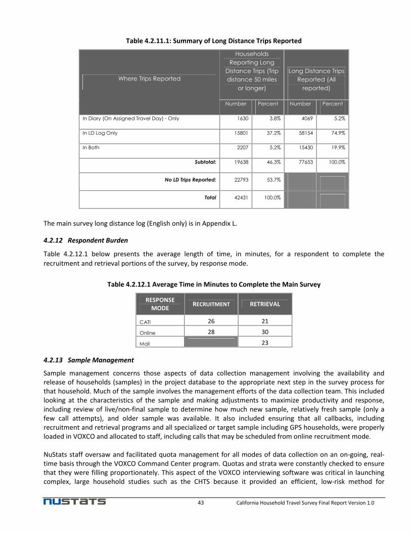
43 California Household Travel Survey Final Report Version 1.0
Table 4.2.11.1: Summary of Long Distance Trips Reported
Where Trips Reported
Households
Reporting Long
Distance Trips (Trip
distance 50 miles
or longer)
Long Distance Trips
Reported (All
reported)
Number Percent Number Percent
In Diary (On Assigned Travel Day) - Only 1630 3.8% 4069 5.2%
In LD Log Only 15801 37.2% 58154 74.9%
In Both 2207 5.2% 15430 19.9%
Subtotal: 19638 46.3% 77653 100.0%
No LD Trips Reported: 22793 53.7%
Total 42431 100.0%
The main survey long distance log (English only) is in Appendix L.
4.2.12 Respondent Burden
Table 4.2.12.1 below presents the average length of time, in minutes, for a respondent to complete the
recruitment and retrieval portions of the survey, by response mode.
Table 4.2.12.1 Average Time in Minutes to Complete the Main Survey
RESPONSE
MODE RECRUITMENT RETRIEVAL
CATI 26 21
Online 28 30
Mail 23
4.2.13 Sample Management
Sample management concerns those aspects of data collection management involving the availability and
release of households (samples) in the project database to the appropriate next step in the survey process for
that household. Much of the sample involves the management efforts of the data collection team. This included
looking at the characteristics of the sample and making adjustments to maximize productivity and response,
including review of live/non-final sample to determine how much new sample, relatively fresh sample (only a
few call attempts), and older sample was available. It also included ensuring that all callbacks, including
recruitment and retrieval programs and all specialized or target sample including GPS households, were properly
loaded in VOXCO and allocated to staff, including calls that may be scheduled from online recruitment mode.
NuStats staff oversaw and facilitated quota management for all modes of data collection on an on-going, real-
time basis through the VOXCO Command Center program. Quotas and strata were constantly checked to ensure
that they were filling proportionately. This aspect of the VOXCO interviewing software was critical in launching
complex, large household studies such as the CHTS because it provided an efficient, low-risk method for

44 California Household Travel Survey Final Report Version 1.0
centralized, timely tracking and adjustments. When necessary, sample was assigned with priority to generate
completes in lagging quota cells.
In addition to sample and quota management, the team closely tracked and managed productivity, production
levels, and schedules on an hourly basis. If productivity was lagging, staff troubleshot project performance and
worked quickly to identify the cause(s) and rectify the issue(s). Proper quota and production management for
large studies such as the CHTS were heavily reliant on real-time, constant sample management so production
task leads were tracking, coordinating, and reporting on sample performance indicators with other key project
team members on a regular basis.
Recruitment Sample Protocols
For the CHTS sample was divided into individual replicates of 500 samples each. Each replicate contained a
random representation of the sample universe. The value of using replicates to manage sample was in having the
ability to fully work through sample within each replicate before moving on to the next one. This allowed the
data collection team to maximize sample performance before releasing new sample to the mix. Some replicates
were also designed to represent various household types (i.e. matched vs. unmatched or GPS vs. Non-GPS
households) and they were loaded into the VOXCO system and released for dialing following a systematic
advance mail out schedule. Note that the timing of the sample release was done in conjunction with when
advance letters had been mailed out, for those households that received advance letters. Toward the end of the
main survey, replicates were created for specific counties and system weights were applied to these replicates so
that the program would release this sample at a higher rate than the rest of the sample. Among other reasons,
this was done to attempt to increase representation of lagging counties.
The CHTS recruitment program contained standard call outcomes and some project specific codes as well.
Interviewers were trained to follow specific protocols in coding call outcomes correctly. Each interviewer were
assigned an interviewer identity number to access the program. This allowed for each call record to be tracked to
the interviewer for review, feedback and coaching opportunities as needed. This was a valuable tool to identify
interviewers that needed help with refusal avoidance techniques or other areas that could be identified by
running interviewer performance statistics.
For the CHTS, a minimum of eight attempts to valid numbers resulting in a no contact were made before
finalizing a sample record. This protocol was adjusted throughout the duration of the project, for example, to
increase the level of effort in lagging areas. In some of the hard to reach areas sample was rested for a long
period of time and re-attempted later in the project. For some of these cases the minimum call attempt was
higher although the calls were spaced out across a longer period of time. In other areas it was necessary to
maintain the number of five call attempts in order to maintain acceptable productivity levels.
One other aspect of sample management was the "rest-and-recycle" technique for non-responsive households.
After eight attempts without being able to contact a household, those samples were "rested" for a period of
three months (or until the end of the quarter), and then were recycled back into the active sample pool for re-
calling and re-contacting.
Retrieval Sample Protocol
A key element to consider when referring to sample management and the retrieval stage was the Production
Schedule. The Production Schedule contained the list of all valid travel dates for the duration of the project. This
schedule dictated when sample needed to be available for reminder calls and when it needed to be available for
retrieval calls.

45 California Household Travel Survey Final Report Version 1.0
Sample management for retrieval was an on-going and hands on task that often times required supervisory and
management staff to discuss sample segments or even specific households on the best approach to finalize the
household. Some of the considerations taken into account included whether the household had been called
during the day of the week and time of the day when the recruitment interview took place, whether calls had
been spread out across times of the day and days of the week, whether any or too many messages had been left,
or whether the household needed to be finalized as non-completed and needed to be replaced.
The Strata and Quotas definition module in VOXCO allowed NuStats to manage subsets of the sample and to
open or close access to any stratum or subset as needed. It also allowed NuStats to apply quotas or ceilings to
control the maximum number of completed interviews by stratum, and the rate at which they were attained.
This module was used for tracking goals and in sample management by assisting in the release or withholding of
specific sample segments. Many of the sample management activities already described were made possible by a
specific strata definition that existed in the Quota Management module. The starting point of making this sample
control tool work was to specify a set of criteria or strata, upon which sample controls or quotas were to be
applied.
For the CHTS, quotas also were used to monitor household distribution across travel days to obtain a
proportional distribution of days of the week and across weeks and months during the full year of data
collection.
There were situations in which there was a need to regulate or balance the rate at which a group of strata were
filled during the course of the project. To achieve this, a probability or weight was assigned to a lagging stratum,
so that the system would increase the rate by which sample from that strata was released. This process was
critical for achieving goals on time, for example when the deadline for closing out a wearable MTC scheduling
date was approaching, adding a weight to the wearable MTC sample ensured more of this sample was called to
increase the chances to meet the goal on time.
4.3 Survey Outreach – Hard to Reach Populations
The CHTS pretest results indicated a lower than desired response rate from Hispanic and low income
populations. At the urging of representatives of the Federal Highways Administration (FHWA) and the CHTS
Administrative Committee, Caltrans sought internal funding for a public outreach effort to improve
representation of these groups in the CHTS main survey effort. The Division of Transportation Planning provided
funding for public outreach efforts. The initial scope of work was circulated in January 2012 and the first meeting
with the contractor was held in April 2012. To provide guidance to the contractor, a technical advisory
committee (TAC) of the Administrative and Steering Committees, the Hard-to-Reach Populations Subcommittee,
was formed and met monthly through November 2012.
Key outreach efforts conducted by the contractor were:
• Developed and provided to Caltrans Public Affairs Office lists of prominent media (print, radio and
television) statewide and focusing on Southern California (developed in June 2012)
• Provided two public service announcements (PSA), in English and in Spanish, to major media
outlets in Southern California. The first paid PSA ran in early October 2012 for 2 weeks in mid-
October and the second ran in early December 2012. Additional PSAs were aired statewide, free of charge, until January 31, 2013.
• Provided Caltrans and SCAG-specific voice over of the MTC video (see below) explaining the survey
process. The revised MTC video was released in early October and posted on the CHTS website as
well as the social media sites.

46 California Household Travel Survey Final Report Version 1.0
• Prepared Speakers Bureau, Press and Community Influentials Kits. Contents of the kits included: a
project brochure, sample news article, Frequently Asked Questions (FAQ) list, fact sheet and
PowerPoint presentation, all in both English and Spanish and in print and on CD. These kits were
finalized in August 2012. The Speaker's Bureau Kits and Press Release Kits were distributed to all
stakeholders upon release of the video in early October 2012.
While the materials developed by the contractor were of high quality, most of the efforts occurred in the third
and fourth quarter of the main survey data collection, so that any impact on participation and response rates
was minimized.
In addition to the Caltrans public outreach contractor, Caltrans and individual MPOs also conducted their own
outreach efforts in their region. Caltrans Public Affairs Division prepared and disseminated press releases about
the CHTS. The most spectacular MPO outreach effort was a video about the CHTS survey and what it entailed for
respondents created by the Bay Area Metropolitan Transportation Commission (MTC). The video was available in
English in March 2012, and in Spanish in April 2012. At the date of this report, the video was available for viewing
on the MTC website in English:
(http://www.mtc.ca.gov/news/press_releases/rel548.htm) and in Spanish:
(http://www.mtc.ca.gov/news/press_releases/rel548_espanol.htm ).
To assist in targeting the outreach effort, NuStats provided quarterly analyses of the recruitment and retrieval
rates for hard-to-reach populations, by county. In general, the hardest to reach groups continued to be Hispanic,
and younger (<25) residents, as well as residents of the larger counties in the state.
4.4 Quality Control
The following quality control protocols were implemented for the CHTS data collection team:
• A comprehensive Interviewer-training (specifically focused on understanding and proper delivery of the CATI
questionnaire)
• Adherence to CASRO guidelines
• Expert program design input and detailed and redundant program testing
• Dedicated, permanent team of Managers, Trainers, Supervisors and Interviewers.
• On-site and off-site monitoring of interviewers’ efforts by project-specific QC leaders. Monitoring capability
used with options of providing instant messaging feedback during live calls.
• On-going, constant dual data reviews being conducted by data collection leaders and by NuStats data
cleaning team throughout the entire data collection period.
• Electronic tracking of interviewers’ performance – dialing statistics, completed interviews, refusals, non-
contacts, average interview lengths.
Live, full monitoring of CATI interviews led by project-dedicated Quality Control Managers and Supervisors were
conducted as the cornerstone of the QC process for this study. Full monitoring sessions, where a conversation
between an interviewer and a respondent is not only heard but also viewed through remote visual monitoring,
were the most efficient and reliable method for ensuring that Interviewers were reading scripts verbatim as well
as accurately recording all data provided by respondents. Following industry guidelines, a minimum of 10% of all
CATI completes were monitored or validated. Monitoring sessions were also used to provide on-going
supplementary training to interviewers as well as to validate the accuracy of the real-time entry. For each
monitoring session, interviewers were evaluated on the following criteria: dialing rate, effective use of time,
professionalism, gaining cooperation, disposition coding, contact procedures, reading verbatim, neutral delivery,

47 California Household Travel Survey Final Report Version 1.0
effective probing, pacing and focus, and accurate data entry. In addition, for retrieval the primary QC focus was
on trip collection, probing for missed trips, and the accuracy of the collection of address details.
In addition, dual project data reviews were also a key part of the overall QC process. On a shift-by-shift basis, the
NuStats QC team actively checked data within the dialing program for completeness on key criteria. This was
followed by full-scale automated data checks by NuStats data staff to confirm that data met the required
specifications. This dual system helped ensure that the NuStats QC team was able to quickly correct any potential
data issues and to also administer immediate remedial training for specific Interviewers.
Figure 4.4.1 shows the full data processing effort, including the quality control measures.
Figure 4.4.1: Data Processing Flow Chart

48 California Household Travel Survey Final Report Version 1.0
5.0 Global Positioning System (GPS) Subsample
5.1 Overview
The purpose of the GPS component of the California Household Travel Survey (CHTS) was to collect detailed
information about all trips made by the GPS subsample and to estimate levels of trip underreporting in this
subsample that can be applied to the larger, non-GPS sample. The following section summarizes the GPS data
collection results for the GPS / Diary Complete households (as defined by the updated GPS and diary completion
rules). All households that reported travel by February 14, 2013 are included. With a target goal of obtaining
5,199 GPS complete households, it was estimated that at least 8,949 households would need to be recruited.
Recruitment for the study concluded on January 18, 2013. There were 9,048 households recruited into the GPS
component of the study. A split design was implemented, with some households receiving in-vehicle GPS devices
and other households receiving wearable GPS devices. The GPS devices were to be used for seven days by the
vehicle sample and three days by the wearable sample, with the first day coinciding with the assigned diary /
travel day. A portion of the vehicle sample was also targeted to receive On-Board Diagnostic (OBD) Engine
Sensors to use in tandem with the vehicle GPS devices to provide additional details about vehicle and engine
activity that could be used, in turn, to estimate fuel consumption and emissions levels.
This split technology design allowed for the collection of seven days of highly accurate vehicle-based data with
minimal respondent burden while limiting the burden of carrying wearable GPS devices to a three-day period.
Households selected for the wearable GPS component were deployed for three days, with all household
members between the ages of 16 and 75 receiving GPS equipment. Local deployment personnel shipped and
received returned equipment from/to their home. As GPS devices were returned by GPS households, the data
collected on the devices were downloaded and posted to the GPS Project Management Website. From there, the
data were imported into the project database and processed by analysts to review and confirm trip end locations
and mode assignments. A $25 incentive per instrumented vehicle or person was offered to all recruited GPS
households for successful reporting of travel data, for use of all GPS devices provided, and for return of all
devices. A $40 incentive per instrumented vehicle was offered to all recruited GPS/OBD households.
GeoStats, as a subcontractor to NuStats, was responsible for implementing the GPS and OBD components of this
survey. A supplemental GPS data deliverable containing all GPS data collected from households that completed
the study after February 14, 2013, which only supplied partially complete data or which collected GPS data, but
did not report their travel, will be generated and delivered before the contract ends on June 14, 2013 as a
separate data set.
5.2 Deployment Methods and Results
5.2.1 Deployment Methods
Given the size and scope of the GPS portion of this study (which was set at approximately 175 households
recruited and deployed per week for one year), it was decided that three persons should be contracted to assist
with equipment deployment — two for wearable deployments and one for vehicle and vehicle OBD
deployments. Deployment staffing was obtained accordingly, with the recruits split between the deployment
team members based on GPS type, geographic location and the availability of equipment.

49 California Household Travel Survey Final Report Version 1.0
Households were recruited into the travel survey at least 10 days prior to their assigned travel date. As GPS
households were recruited, recruit details were pulled such as names, addresses, phone numbers, and person
and vehicle rosters. This recruit information was imported into the database and the deployment zone was
assigned based on the GPS type and the split between the deployment team members. This recruit information
was then made available on the GPS Study Management website, where each deployment person accessed the
recruit information for only their assigned shipments.
The deployment team members signed onto the password-protected website on a daily basis to review
upcoming deployments. The lead time between the posting of recruited households to the website and the
assigned travel date was at least seven days, allowing sufficient time to prepare the necessary documents,
diaries, and equipment, and to ship them to arrive prior to the assigned travel date.
Simple printed instructions were shipped with the devices; these instructions also listed the assignment of each
logger to each household vehicle or household member (for either the vehicle or wearable GPS sample) based on
the logger identification number. In addition, a hotline phone number was provided to the respondent for
assistance with installation and use of the devices. A sticker was affixed to each GPS device with the vehicle year
and model for households recruited into the vehicle study or the first name of the household member printed on
the sticker for households recruited into the wearable study. The instructions also emphasized the need to use
the diaries to record travel on the assigned travel date. A return device sheet was also provided on which the
household members were asked to record if they used the devices, and if not, to list the reason(s) why.
Shipping was conducted via FedEx. Participant instructions, equipment, diaries and a pre-paid return FedEx Pak
were placed in a cardboard box and secured with packing material. The equipment was delivered to the
household two business days prior to the assigned travel day. After the assigned GPS data collection period,
households were to place all of the equipment and the return device sheet in the original box, insert that box in
the FedEx Pak, and put either the package into a FedEx drop box or call 1-800-GoFedEx to schedule a pick-up at
their home. Outbound and return equipment packages were tracked on the FedEx website, with tracking
information loaded on the GPS Study Management website. The participants were requested to hold onto their
diaries, either reporting travel over the phone, via the project website or return the diaries in the pre-paid return
envelope provided with the diaries.
The deployment team was instructed to prepare and ship equipment packages for each household listed for
them on the GPS Study Management website. Project management communicated with the deployment team
on a regular basis to ensure that each member had sufficient equipment supplies to meet the upcoming
deployment needs. The deployment team members were instructed to update the household deployment status
on the website as the statuses changed. The default status for deployment when recruit information was first
loaded was ‘Recruit’. They would then change this status to reflect the current state of the deployment process.
Below is a list of all household deployment status codes: the first four statuses reflect the natural progression of
a successful deployment, whereas the final four statuses reflect GPS recruits that did not result in a useful
deployment.
• Recruited
• Shipped
• Deployed
• Returned Deployed (used and returned equipment)
• Invalid Address
• Returned Refused (elected not to participate)

50 California Household Travel Survey Final Report Version 1.0
• Return-Delivery Exception (package unable to be delivered by FedEx)
• Not Returned / Lost
After receiving the returned equipment, the deployment staff downloaded the GPS raw data from the loggers
and then cleared the device memory for redeployment. The downloaded, zipped GPS file was then posted to the
project website and imported into the project database, from where all further GPS data processing occurred.
Deployment personnel were also responsible for updating the person-level equipment usage status fields as
reported by each household, for recording any household or person-level comments on the website, and for
updating the household level control code. A 10% sample from the GPS raw data has been supplied to NuStats
on a quarterly basis.
Wearable GPS Equipment
The GlobalSat GPS Data Logger is a rugged yet simple GPS data logging device (see Figure 5.2.1.1Figure). The
GlobalSat device weighs 6 oz. and has dimensions of 2.75”x3.15”x.7”. It can be worn on the waist, clipped to a
purse or backpack, or dropped in a suit jacket pocket.
This device can log at various frequencies, can log all valid GPS points or only those valid points for which the
speed is greater than one MPH (to screen out non-movement events), and has a 100,000 GPS point storage
capacity. For the purpose of this study, the logging frequency was three-second intervals with the speed screen
activated. The GPS data stream elements recorded by the GlobalSat for this study included date, time, latitude,
longitude, speed, heading, horizontal dilution of precision (HDOP), and number of satellites. These elements are
stored in the logger in standard NMEA units and are converted into user-specified units and formats upon
download. At the start of the study, 1,476 GlobalSat devices were provided to support deployment of 6,141
households over the 12-month main survey data collection period.
Figure 5.2.1.1: GlobalSat DG-100 GPS Data Logger
In-Vehicle GPS Equipment
The QStarz BT-Q1000x Travel Recorder (Figure 5.2.1.2) was used for the in-vehicle GPS component of this study.
This device captures date, time, latitude, longitude, speed, and other standard GPS variables in one-second
intervals, and can be configured to collect additional variables including heading, horizontal dilution of precision
(HDOP), and number of satellites. This device entered the market in 2009 in and has been successfully deployed
in two recent large-scale household travel surveys, and several other transportation related projects. In the
California Statewide Travel Survey, this device was provided to participants with a vehicle power cable and
power splitter so that participants could also charge other personal devices if needed. The power cable also has a
small suction cup attached so that the participant could secure the cable and device on the dashboard near the
windshield to prevent slippage. GeoStats provided 720 QStarz BT-Q1000x devices to support the deployment of
2,808 households to meet the in-vehicle (including OBD) GPS deployment goals for the study.

51 California Household Travel Survey Final Report Version 1.0
Figure 5.2.1.2: QStarz BT-Q1000X Travel Recorder
On-Board Diagnostic Sensor
The CarChip Fleet Pro On-Board Diagnostic Sensor (OBD) seen in Figure 5.2.1.3 was used for the in-vehicle GPS
with OBD component of this study. The device parameters were limited to five and the firmware was customized
to capture speed, air flow rate, throttle position, engine load and engine speed in 5-second intervals. These
variables can be used to identify modal profiles (idle, cruise, acceleration and deceleration) which can, in turn, be
used with existing emission rate models to forecast green house gas (GHG) emissions and fuel use. Participants
were asked to insert this device into the diagnostic port in their vehicle, which is typically located under the dash
on the driver side of the vehicle. Once installed, the device records data whenever the vehicle is powered on. The
OBD device does not require external charging. GeoStats provided 573 CarChip Fleet Pro devices to support the
deployment of 2,106 households to meet the in-vehicle GPS and OBD deployment goals for the study.
Figure 5.2.1.3: CarChip Fleet Pro On-board Diagnostic Engine Sensor
5.2.2 Deployment Results
Equipment was deployed to 8,994 households. An equipment retrieval management system was developed and
used to coordinate follow up with all GPS households that did not immediately return their GPS equipment as
instructed. First, a phone call was placed to the home telephone number for all households that did not return
their GPS devices within one week after the last GPS travel date. When a person answered or an answering
machine picked up, a message was delivered thanking the household for their participation and requesting that
the GPS equipment be returned in the pre-paid FedEx envelope. A toll-free call back number was left if the
household had any questions. If no person or answering machine was reached, additional calls were attempted.
If equipment still had not been placed into the FedEx system by two weeks after the last GPS travel day, a letter
was sent to the home. A second equipment retrieval letter was mailed to the household if equipment was still
outstanding after four weeks. During the final week of the study, phone calls were made and letters were mailed
simultaneously in an attempt to retrieve as much equipment as possible. At the time of this report, 337
households across all GPS types (3.74% of total households) had not returned the GPS devices sent to them.
In addition to tracking deployments by GPS type, households were also tracked by funding source. The Core
households refer to those that were funded by Caltrans and their partners and were tracked at the statewide and

52 California Household Travel Survey Final Report Version 1.0
county level. Two agencies provided additional funding, and specified that that funding be spent to collect
additional GPS data of interest to their agency. The Metropolitan Transportation Commission (MTC), the
planning organization for the nine-county San Francisco Bay area provided funding for an additional 3,099
wearable GPS households to be deployed in their region. The California Energy Commission (CEC) provided
funding for in-vehicle GPS and OBD of 500 households that currently own alternative and renewable fuelled
vehicles. The CEC sample was limited to households that owned one or more of the following vehicles: hybrid,
clean diesel, battery electric, plug-in hybrid electric vehicle, CNG, flex-fuel (E85), and Hydrogen vehicles. The
deployment outcomes by GPS Type and funding source are in Table 5.2.2.1.
Table 5.2.2.1: Deployment Statistics by GPS Household Sample Type
Sample Type Recruited Returned
Deployed
Refused Not
Returned
Not
Deployed
Core Wearable GPS 633 524 83 17 9
Core Vehicle GPS 700 563 92 38 7
Core Vehicle GPS / OBD 1,299 1,031 195 56 17
MTC Wearable GPS 5,608 4,534 848 207 19
Energy Commission Vehicle GPS /
OBD 809 726 61 19 3
Total 9,049 7,378 1,279 337 55
5.2.3 GPS Participation Results
Once the GPS trip processing and GPS / diary matching steps are finished, complete and accurate GPS trip details
are available. These details include trip start and end times, origin and destination coordinates, travel distances
and paths, and average speeds for each trip detected. These GPS data sets contain data for the 8,202 persons
instrumented in the 3,871 GPS/diary complete households (that received wearable GPS devices) and for 3,491
vehicles in the 1,684 GPS/diary complete households (that received vehicle GPS or GPS/OBD devices) for which
data were received by February 2013. The data deliverable contains 204,634 trips covering 1,265,986 miles
traveled and 2,660,505 travel minutes (44,342 hours). Table 5.2.3.1 shows the recruitment and completion
statistics included in this data deliverable.
Table 5.2.3.1: Recruitment, Completion and Results by GPS Household Type
Sample Type Recruit
Total
Recruit
Goal
Recruit %
Complete
GPS/Diary
Complete
GPS/Diary
Complete
Goal
%Complete
Goal
Core Vehicle GPS 700 702 100% 424 400 106%
Core Vehicle GPS / OBD 1,397 1,404 100% 902 800 113%
Core Wearable GPS 633 702 90% 420 400 105%
MTC Wearable GPS 5,608 5,439 103% 3,451 3,099 111%
Energy Commission Vehicle GPS / OBD 711 702 100% 540 500 108%
Total 9,049 8,949 101% 5,737 5,199 110%
There is no disposition of all households participating in the GPS component by study type table because this
report includes data for only those households which completed all portions of the study.

53 California Household Travel Survey Final Report Version 1.0
5.3 GPS/Diary Processing Methods and Results
As the GPS data collected by the participants were imported into the project database, the UTC (Universal Time
Coordinate) date and time stamps in the GPS point data were translated to local date and time. As mentioned
previously, the speed filter settings on both the in-vehicle and wearable GPS Data Loggers deployed to study
participants were set to screen out all zero point speeds, with non-zero speed points recorded at a one-second
frequency for in-vehicle devices and at a three-second frequency for wearable devices.
Next, each GPS file was processed using Trip Identification and Analysis System (TIAS) software to identify
potential trip ends based on time intervals between consecutively logged points. For this study, all initial dwell
times of 120 seconds or more were flagged as potential trip stops. The GPS trip data were then visually reviewed
by analysts to screen out traffic delays and other falsely identified stops with dwell times of 120 seconds or
more, as well as to add stops that had dwell times of less than 120 seconds but had clear “stop” characteristics.
Examples of typical stops that would not be automatically detected by the 120 second dwell time are short drop-
off/pick-ups (i.e. school, work, mail, ATM, fast food). If geocoded addresses were available from either the recruit
call (i.e. habitual destinations such as home, work and school locations) or from the retrieval call (i.e. each
reported destination made by each household member) then the analyst used these locations to assist in the trip
end identification and/or confirmation process. Once this step was completed, the updated GPS-based trips
collected were ready to be compared and matched with the diary trips reported for that same person or vehicle
on the assigned travel day. Figure 5.3.1 shows an example (non-participant data) of a walk, bus, walk trip in TIAS.
Figure 5.3.1: TIAS Interface Showing Walk-Vehicle-Walk Trip
The travel modes for each activity segment were assigned using TIAS’ mode assignment algorithms and update
interface, and are included as part of the data delivery. TIAS assigned the travel modes based on the GPS trip's
speed profile. Analysts then reviewed each trip trace to confirm or update the mode assignment. The travel

54 California Household Travel Survey Final Report Version 1.0
modes available for assignment in this study were walk, bicycle, auto/truck, bus/train, vanpool and other (see
Figures 5.3.1 and 5.3.2).
Figure 5.3.1: Speed Profiles of Travel Modes – Walk and Personal Auto Trip
Walk Trip
Personal Auto Trip

55 California Household Travel Survey Final Report Version 1.0
Figure 5.3.2: Speed Profiles of Travel Modes – Bicycle and Bus Trip
Bicycle Trip
Bus Trip
5.4 OBD Data Collection and Processing
Like the GPS data, the OBD data files were downloaded from the devices in the field, and then uploaded to a
secure website. The files were then download and imported into the secure project database daily. GeoStats
worked with Davis Instruments, the OBD device manufacturer and vendor, to customize the data recording
configuration for the OBD devices used in the study. They were configured to record speed at a one-second
frequency and four additional parameters at a six-second frequency. See Table 5.4.1 for the recording
configuration by parameter. Davis instruments has confirmed that the device logging interval can vary depending
on the vehicle response, and can be absent from some or all trip records on any given vehicle. More discussion
on OBD quality checks is included later in this section.

56 California Household Travel Survey Final Report Version 1.0
Table 5.4.1: OBD Device Configuration Parameters
Parameter
Recording
Interval
Unit
System Units Decimals
Range
Vehicle Speed 1 sec Metric km/h 0 0-255
(Mass) Air Flow rate 6 sec S. I. kg/s 3 0-65.5
Engine Load 6 sec N/A % 1 0-100
Engine Speed 6 sec U. S. RPM 0 0-16,384
Throttle Position 6 sec N/A % 1 0-100
There were additional data elements queried at lower frequencies and reported as available by vehicle. The full
list of other recorded variables types (which vary by vehicle) for the custom OBD configurations are listed below.
These variable types and additional information about them can be found in the OBD data dictionaries, GPS/OBD
and Raw OBD.
• Activity records-device activity such as plugged into vehicle, unplugged from vehicle, emissions censors
checked
• Activity record readiness codes—only recorded when activity record event type is 8. The list of codes is
defined in the data dictionary
• Diagnostics Trouble Codes (DTC) records
• Trip start and Trip end
• Trip duration
• Vehicle Identification Number (VIN)
• Vehicle Protocol
• Max speed
• Average speed
• Trip distance
• Hard brake, hard acceleration, extreme brake, extreme acceleration counts
• Speed records—speed record for each of the hard and extreme brake and acceleration events
• Malfunction Indicator Light (MAL)—distance with MAL on, distance since Diagnostic Trouble Codes
cleared
• Fuel Type—Type of fuel, % of ethanol in fuel
The Vehicle table in the GPS/OBD deliverable contains several fields related to Vehicle Fuel Type. The ‘fueltype’
field contains the data records reported on the OBD device. Fuel type is not a mandated OBD parameter (not all
vehicles report this value) therefore there were only 61 vehicles in the sample that returned a valid fuel type
codes. Table 5.4.2 contains the list of possible fuel types collected by the OBD device.
Table 5.4.2: Fuel Type Codes from OBD Device
Fuel Type Code from OBD Device:
00 Unknown
01 Gasoline
02 Methanol
03 Ethanol
04 Diesel
05 LPG

57 California Household Travel Survey Final Report Version 1.0
Fuel Type Code from OBD Device:
06 CNG
07 Propane
08 Electric
09 Bifuel running Gasoline
0A Bifuel running Methanol
0B Bifuel running Ethanol
0C Bifuel running LPG
0D Bifuel running CNG
0E Bifuel running Prop
0F Bifuel running Electricity
10 Bifuel mixed gas/electric
11 Hybrid gasoline
12 Hybrid Ethanol
13 Hybrid Diesel
14 Hybrid Electric
15 Hybrid Mixed fuel
16 Hybrid Regenerative
The VEHT and FUELT field records were provided by the participants during the recruitment interview. The codes
and potential responses (from the recruitment script) for these items are in the Table 5.4.3 and were used to
create Table 5.4.4 (Fuel Type by Vehicle Type table).
Table 5.4.3: Diary Reported Vehicle Type and Fuel Type
VEHT (vehicle type) Response
1 Hybrid Vehicle FUELT [PROG: SHOW ALL]
2 Gasoline Only Vehicle FUELT=1
3 Diesel Only Vehicle FUELT [PROG: SHOW ONLY CHOICES 2 & 5]
4 Plug In Hybrid Electric Vehicle FUELT [PROG: SHOW ALL]
5 CNG FUELT=4
6 Electric Only FUELT=3
7 OTHER FUELT [PROG: SHOW ALL]
FUELT (Fuel Type)
1 Gasoline
2 Diesel
3 Electric/Electric Battery
4 CNG - Natural Gas
5 Biofuel, Ethanol, Biodiesel
7 OTHER, SPECIFY (O_FUELT)
8 DK
9 RF
Table 5.4.4 contains the final summary of OBD vehicles (core and Energy Commission sample) by diary reported
vehicle type and / or fuel type from households which were considered complete. It includes the sample source,
the recruit and complete totals, as well as the percentage of recruited and complete vehicles by fuel type.

58 California Household Travel Survey Final Report Version 1.0
Table 5.4.4: Fuel Type by Vehicle Type for OBD Vehicles (Core and Energy Commission add-on)
Fuel Type VEHT
FUELT
(multiple
response)
Sample
Source
# Vehicles
Recruited
# Vehicles GPS
& diary
complete HHs
% Total
REC by
FUELT
% Total
COMP by
FUELT
Gasoline 2 1
Core 2251 1454
78% 76% DMV 730 532
UCD 81 74
Hybrid
Electric/Gasoline 1 1 & 3
Core 112 83
12% 12% DMV 319 248
UCD 26 24
Flex Fuel
(Ethanol/Gasoline) 7 1 & 5
Core 13 8
1% 1% DMV 12 9
UCD 0 0
Diesel 3 2 & 5
Core 67 43
4% 4% DMV 89 69
UCD 1 1
Primary Natural Gas 5 4
Core 1 1
1% 1% DMV 40 30
UCD 2 2
Primary Electric 6 3
Core 4 4
4% 4% DMV 33 26
UCD 101 86
PHEV 4 1 & 3
Core 0 0
1% 1% DMV 17 15
UCD 7 6
Total Vehicles
Core 2448 1592
DMV 1239 929
UCD 218 194
Grand Total 3905 2715
Table 5.4.5 includes the vehicle summary of OBD vehicles (core and Energy Commission sample) by diary
reported vehicle type and / or fuel type by geographic distribution from households which were considered
complete. Certain fuel types were targeted by geography. For instance, the highest density of E85 retail stores
are located in the Sacramento area, therefore the portion of Energy Commission sample identified as Flex Fuel
vehicles registered in the Sacramento area were targeted.
Table 5.4.5: OBD Vehicle Summary by Fuel Type and County
County Hybrid Gasoline Diesel PHEV
Natural
Gas Electric
Flex
Fuel TOTAL
ALAMEDA 25 67 4 2 0 8 1 107
ALPINE 0 3 0 0 0 0 0 3
AMADOR 0 8 0 0 0 1 0 9
BUTTE 2 19 1 0 0 1 0 23
CALAVERAS 1 8 0 0 0 1 0 10
COLUSA 0 1 0 0 0 0 0 1
CONTRA COSTA 18 63 1 0 0 7 0 89

59 California Household Travel Survey Final Report Version 1.0
County Hybrid Gasoline Diesel PHEV
Natural
Gas Electric
Flex
Fuel TOTAL
DEL NORTE 0 11 1 0 0 0 0 12
EL DORADO 5 42 1 0 0 0 0 48
FRESNO 8 55 0 0 0 0 1 64
GLENN 0 6 1 0 0 0 0 7
HUMBOLDT 1 9 1 0 0 0 0 11
IMPERIAL 0 9 1 0 0 0 0 10
INYO 0 9 0 0 0 0 0 9
KERN 0 51 3 0 2 1 0 57
KINGS 0 4 0 0 0 0 0 4
LAKE 3 11 3 0 0 0 0 17
LASSEN 0 15 1 0 0 0 0 16
LOS ANGELES 73 320 19 5 12 22 4 455
MADERA 1 19 1 0 0 0 0 21
MARIN 4 11 1 0 0 2 0 18
MARIPOSA 0 18 2 0 0 0 1 21
MENDOCINO 1 10 3 0 0 0 0 14
MERCED 0 24 0 0 0 0 0 24
MODOC 0 2 0 0 0 0 0 2
MONO 0 8 1 0 0 0 0 9
MONTEREY 4 15 1 0 0 0 0 20
NAPA 2 9 1 0 0 0 0 12
NEVADA 2 8 0 0 0 0 0 10
ORANGE 24 136 6 1 4 14 0 185
PLACER 4 35 5 3 0 4 0 51
PLUMAS 0 6 1 0 0 0 0 7
RIVERSIDE 11 110 7 1 7 2 0 138
SACRAMENTO 22 120 4 0 0 3 9 158
SAN BENITO 1 21 0 0 0 0 0 22
SAN
BERNARDINO 9 99 6 0 0 0 0 114
SAN DIEGO 28 132 7 2 0 7 3 179
SAN FRANCISCO 7 18 2 0 0 1 0 28
SAN JOAQUIN 1 33 2 0 0 0 1 37
SAN LUIS OBISPO 3 28 1 0 0 1 0 33
SAN MATEO 17 26 1 2 1 7 0 54
SANTA BARBARA 0 28 1 0 0 0 0 29
SANTA CLARA 31 83 4 2 4 18 0 142
SANTA CRUZ 8 41 3 0 0 7 1 60
SHASTA 0 3 4 0 0 0 0 7
SIERRA 1 11 0 0 0 0 0 12
SISKIYOU 0 4 1 0 0 0 0 5

60 California Household Travel Survey Final Report Version 1.0
County Hybrid Gasoline Diesel PHEV
Natural
Gas Electric
Flex
Fuel TOTAL
SOLANO 6 23 0 0 0 1 0 30
SONOMA 7 27 4 1 0 1 0 40
STANISLAUS 2 17 0 0 0 0 0 19
SUTTER 0 11 0 0 0 0 0 11
TEHAMA 1 4 0 0 0 0 0 5
TRINITY 0 27 1 0 0 0 0 28
TULARE 3 50 2 0 0 1 1 57
TUOLUMNE 0 9 2 0 0 0 0 11
VENTURA 14 79 2 0 0 4 1 100
YOLO 4 32 0 0 0 2 0 38
YUBA 0 12 0 0 0 0 0 12
354 2060 113 19 30 116 23 2715
To increase the number of Electric and Plug-in Hybrid Electric vehicles sampled for the study, the Energy
Commission teamed with the University of California, Davis to recruit from a pool of EV and PHEV owners. Due
to the newness of the technology and the lack of a combustion engine in all-electric vehicles, EVs and PHEVs do
not support OBD devices. For these vehicles, GeoStats sent a paper survey (in place of an OBD device), designed
by UC Davis, to EV and PHEV vehicle households to collect vehicle data. These paper surveys were collected by
GeoStats, entered into the OBD database and provided as part of the OBD data deliverable.
As a quality control measure the date and timestamps present on the GPS trips were compared to the data and
timestamp on the OBD trips to ensure that they were synchronized. As part of the OBD data monitoring process
the data were checked to confirm that all data elements imported and were accurate. As mentioned previously,
the OBD parameters and vehicle reporting can vary among vehicles depending on the make, model, and year.
For example, VIN was not a mandated parameter until 2003 so only 52% of vehicles (1,411 out of 2,715) returned
a valid VIN number. Likewise, some vehicles do not report one or more of the four 6-second interval parameters
(i.e. Mass Air Flow Rate). To more easily identify OBD trips that had failed parameter data collection, a set of
flags were created in the OBD Trips table. The OBD data dictionary contains a complete list of these flags and
parameters. Beyond these quality control / monitor steps no comparison was conducted between the variables
captured by GPS and OBD devices. The raw OBD data were stored and monitored, but not processed.
5.5 GPS and Diary Trip Matching Results
This data deliverable includes all ‘GPS / DIARY complete’ GPS households. There are a total of 3,491 GPS vehicles
in the 1,866 complete vehicle and vehicle OBD GPS households and 8,202 GPS persons in the 3,871 wearable GPS
households. The 3,491 GPS vehicles captured 12,380 GPS trips on the assigned travel days, compared to 11,609
reported trips for these same vehicles. The 8,202 GPS persons captured 45,986 GPS trips on their assigned travel
day compared to 39,995 reported trips for these same participants. So, across all GPS samples, a total of 58,366
GPS trips were collected compared to 51,604 reported trips for the same vehicles or persons.
5.5.1 Reporting Exceptions
In some household travel surveys, work-related trips (i.e., commercial use of personal auto) and external to
external trips (i.e., those that have origins and destinations outside of the planning regions) are not reported in
the travel diary and not collected during the retrieval call. These were the instructions for this study as well.

61 California Household Travel Survey Final Report Version 1.0
Other typical unreported trip types include loop trips (i.e., those that start and end at the same location) and on-
site travel (i.e. trips that are conducted on the premises of one property, like a hospital or apartment complex).
However, of the 1,120 external to external GPS trips that were detected in the GPS/CATI complete households,
1,057 of these trips were reported. Similarly, of the 3,055 work-related GPS trips found in these households,
2,066 had been reported. This left a total of 63 external-external trips and 989 work-related trips found in the
GPS data that had not been reported (and were not required to be reported).
GPS trips were flagged as loop trips whenever a GPS trip was detected in which the origin and destination were
the same location. According to the rules of this study, loop trips should have been reported whenever their
purpose (e.g., exercise or walk the dog) was not tied to the purpose of the previous trip. This means that a loop
trip made from home is a valid trip whereas a loop walk trip in a park preceded by a drive to the park for exercise
purposes should not have been reported. A total of 2,637 loop trips were identified, 1,969 of which were
reported by participants. Furthermore, 3,797 other non-transportation or on-site trips were found that were not
required to be reported.
Even though participants in this study were instructed to report all trips except for work-related and external to
external trips, it is likely that some participants also did not report loop and on-site trips as well. The remainder
of the missed trip analyses will presents results that include the raw and adjusted frequencies. The adjusted
frequencies removed work-related, external to external, loop and on-site travel trips if they did not have
matching reported trips.
5.5.2 Matching Results - Wearable
The results of the trip matching process for the GPS sample fell into the following three categories:
100% Matched Trips. Any person instrumented with GPS that captured the same GPS trips as reported by diary
were considered to be a perfect match. This category also includes no travel persons which had no GPS data
collected on the travel date and no trips reported for that person on the assigned travel date. Of the 8,202
persons instrumented with GPS devices in the 3,871 GPS/diary complete households, 964 persons had no GPS
data and were confirmed as no travel in the diary data (11.8% of all instrumented persons).
1. Of all trips made by the 6,241 instrumented persons, 3,050 persons had perfect matches between the
diary and GPS trip data. The breakdown of this number includes the 964 persons who did not travel and
2,086 persons who made at least one trip. This represents a perfect match (or reporting rate) for 37.2%
of all instrumented persons in GPS/Diary complete households and 19,266 of the 38,129 diary-reported
trips (50.5%). Table 5.5.2.1 contains the trip frequency statistics for the persons included in this
category.

62 California Household Travel Survey Final Report Version 1.0
Table 5.5.2.1: Trip Frequencies for Perfect Matches at Person Level
2. Trips reported by diary but not captured by GPS. The second comparison identifies diary trips that had no
corresponding GPS trips. During the matching process, 5,757 diary trips were identified that had no
corresponding GPS trip (which represents 13.1% of all GPS trips). This typically happens when participants
place the GlobalSat device in a position in which it cannot receive GPS satellite signals (such as in a purse or
backpack) or forget to carry the device, or confirm that it is powered on.
3. Trips captured by GPS but not reported by diary. The last category in the matching process contains those
cases where trips were identified within the GPS data stream but not within the diary data. These 11,725
“missed” diary trips were either single links within a trip chain, multiple links within a trip chain, or
complete round-trips missing all links in a tour, based on characteristics of adjacent trips. Based on the
total of 38,129 diary trips reported, the missing 11,725 diary trips reflect a 30.8% missing trip rate across
the entire sample. However, when the typical reporting exceptions are excluded from this analysis, the
missed trip rate falls to 21.5% for the GPS sample.
Table 5.5.2.2 shows the frequency of missing GPS and diary trip counts detected for the 5,152 persons who
were not perfect matches.
Trips (#) Frequency Frequency (%) Cumulative (%)
0 964 31.6% 31.6%
1 11 0.4% 32.0%
2 485 15.9% 47.9%
3 254 8.3% 56.2%
4 351 11.5% 67.7%
5 249 8.2% 75.9%
6 241 7.9% 83.8%
7 148 4.9% 88.6%
8 129 4.2% 92.9%
9 72 2.4% 95.2%
10 55 1.8% 97.0%
11 34 1.1% 98.1%
12 16 0.5% 98.7%
13 16 0.5% 99.2%
14 8 0.3% 99.4%
15 5 0.2% 99.6%
16 3 0.1% 99.7%
17 3 0.1% 99.8%
18 2 0.1% 99.9%
19 1 0.0% 99.9%
21 1 0.0% 99.9%
23 1 0.0% 100.0%
25 1 0.0% 100.0%
Totals 3,050 100.0% 100.0%

63 California Household Travel Survey Final Report Version 1.0
Table 5.5.2.2: Trip Frequencies for Missing Trips – Wearable GPS
Missing Trips
(#)
Missing GPS
Frequency
Missing Diary
Frequency Raw
Missing Diary Frequency
Adjusted
1 845 1373 1255
2 1288 1608 1482
3 963 1437 1170
4 788 1420 1048
5 575 1050 725
6 408 930 630
7 224 700 392
8 224 496 416
9 126 459 261
10 130 320 120
11 88 253 110
12 24 240 96
13 26 221 143
14 0 210 84
15 15 120 45
16 16 64 0
17 17 102 17
18 0 72 36
19 0 57 19
20 0 60 20
21 0 42 42
22 0 22 22
23 0 46 0
24 0 48 0
25 0 0 0

64 California Household Travel Survey Final Report Version 1.0
Missing Trips
(#)
Missing GPS
Frequency
Missing Diary
Frequency Raw
Missing Diary Frequency
Adjusted
26 0 52 26
27 0 27 0
28 0 0 0
29 0 29 0
30 0 30 0
31 0 93 0
32 0 0 0
33 0 33 0
36 0 36 36
75 0 75 0
Totals 5,757 11,725 8,195
5.5.3 Matching Results – Vehicle
100% Matched Trips. Any vehicle instrumented with GPS that captured the same GPS trips as reported by diary
were considered to be a perfect match. This category also includes vehicles which had no GPS data collected on
the travel date and no trips reported for that vehicle on the assigned travel date. Of the 776 vehicles
instrumented with GPS devices in the 424 GPS/diary complete households, 232 vehicles had no GPS data and
were confirmed as no travel in the diary data (29.9% of all instrumented vehicles).
1. Of all trips made by the 776 instrumented vehicles, 481 vehicles had perfect matches between the diary
and GPS trip data. The breakdown of this number includes the 232 vehicle that did not travel and 249
vehicles that made at least one trip. This represents a perfect match (or reporting rate) for 62.0% of all
instrumented vehicles in GPS/Diary complete households and 1,003 of the 2,318 diary-reported trips
(43.3%). Table 5.5.3.1 contains the trip frequency statistics for the vehicles included in this category.

65 California Household Travel Survey Final Report Version 1.0
Table 5.5.3.1: Trip Frequencies for Perfect Matches at Vehicle Level
Trips
(#) Frequency
Frequency
(%)
Cumulative
(%)
0 232 48.2% 48.2%
1 4 0.8% 49.1%
2 80 16.6% 65.7%
3 36 7.5% 73.2%
4 47 9.8% 83.0%
5 32 6.7% 89.6%
6 20 4.2% 93.8%
7 8 1.7% 95.4%
8 9 1.9% 97.3%
9 7 1.5% 98.8%
10 1 0.2% 99.0%
11 3 0.6% 100.0%
12 0 0.0% 100.0%
13 1 0.2% 100.0%
14 0 0.0% 100.0%
15 0 0.0% 100.0%
16 1 0.2% 100.0%
17 0 0.0% 100.0%
Totals 481 100.0% 100.0%
2. Trips reported by diary but not captured by GPS. The second comparison identifies diary trips that had no
corresponding GPS trips. During the matching process, 159 diary trips were identified that had no
corresponding GPS trip (which represents 5.8% of all GPS trips). This typically happens when participants
place the GPS device in a position in which it cannot receive GPS satellite or forget to confirm that it is
powered on.
3. Trips captured by GPS but not reported by diary. The last category in the matching process contains those
cases where trips were identified within the GPS data stream but not within the diary data. These 567
“missed” diary trips were either single links within a trip chain, multiple links within a trip chain, or
complete round-trips missing all links in a tour, based on characteristics of adjacent trips. Based on the
total of 2,318 diary trips reported, the missing 567 diary trips reflect a 24.5% missing trip rate across the
entire sample. However, when the typical reporting exceptions are excluded from this analysis, the missed
trip rate falls to 22.1% for the GPS sample.
Table 5.5.3.2 shows the frequency of missing GPS and diary trip counts detected for all vehicles that were not
perfect matches.

66 California Household Travel Survey Final Report Version 1.0
Table 5.5.3.2: Trip Frequencies for Missing Trips – Vehicle GPS
Missing Trips
(#)
Missing GPS
Frequency
Missing Diary
Frequency Raw
Missing Diary
Frequency
Adjusted
1 44 100 94
2 34 43 45
3 24 23 26
4 24 27 21
5 15 7 6
6 0 6 6
7 1 3 3
8 0 5 5
9 0 3 2
10 0 1 1
11 1 1 1
24 0 1 0
Totals 159 567 512
5.5.4 Matching Results – Vehicle / OBD
100% Matched Trips. Any vehicle instrumented with GPS that captured the same GPS trips as reported by diary
were considered to be a perfect match, regardless of the presence of OBD data, as defined by the data
completion rules. This category also includes vehicles which had no GPS data collected on the travel date and no
trips reported for that vehicle on the assigned travel date. Of the 2,715 vehicles instrumented with GPS devices
in the 1,442 GPS/diary complete households, 670 vehicles had no GPS data and were confirmed as no travel in
the diary data (24.7% of all instrumented GPS/OBD vehicles).
1. Of all trips made by the 2,715 instrumented vehicles, 1,504 vehicles had perfect matches between the
diary and GPS trip data. The breakdown of this number includes the 670 vehicle that did not travel and 834
vehicles that made at least one trip. This represents a perfect match (or reporting rate) for 55.4% of all
instrumented vehicles in GPS/Diary complete households and 3,548 of the 7,631 diary-reported trips
(46.5%). Table 5.5.4.1 contains the trip frequency statistics for the vehicles included in this category.

67 California Household Travel Survey Final Report Version 1.0
Table 5.5.4.1: Trip Frequencies for Perfect Matches– OBD Households
Trips
(#) Frequency
Frequency
(%)
Cumulative
(%)
0 670 44.5% 44.6%
1 10 0.7% 45.2%
2 243 16.2% 61.4%
3 135 9.0% 70.4%
4 135 9.0% 79.3%
5 113 7.5% 86.8%
6 66 4.4% 91.2%
7 39 2.6% 93.8%
8 45 3.0% 96.8%
9 17 1.1% 97.9%
10 12 0.8% 98.7%
11 5 0.3% 99.1%
12 7 0.5% 99.5%
13 2 0.1% 99.7%
14 3 0.2% 99.9%
15 1 0.1% 99.9%
18 1 0.1% 100.0%
Totals 1,504 100.0% 100.0%
2. Trips reported by diary but not captured by GPS. The second comparison identifies diary trips that had no
corresponding GPS trips. During the matching process, 478 diary trips were identified that had no
corresponding GPS trip (which represents 5.5% of all GPS trips). This typically happens when participants
place the GPS device in a position in which it cannot receive GPS satellite or forget to confirm that it is
powered on.
3. Trips captured by GPS but not reported by diary. The last category in the matching process contains those
cases where trips were identified within the GPS data stream but not within the diary data. These 1,582
“missed” diary trips were either single links within a trip chain, multiple links within a trip chain, or
complete round-trips missing all links in a tour, based on characteristics of adjacent trips. Based on the
total of 7,631 diary trips reported, the missing 1,582 diary trips reflect a 20.7% missing trip rate across the
entire sample. However, when the typical reporting exceptions are excluded from this analysis, the missed
trip rate falls to 18.4% for the GPS/OBD sample.

68 California Household Travel Survey Final Report Version 1.0
Table 5.5.4.2 shows the frequency of missing GPS and diary trip counts detected for the 1,211 GPS/OBD vehicles
that were not perfect matches.
Table 5.5.4.2: Trip Frequencies for Missing Trips – Vehicle GPS (OBD)
Missing Trips
(#)
Missing GPS
Frequency
Missing Diary
Frequency Raw
Missing Diary
Frequency
Adjusted
1 118 303 277
2 74 140 131
3 27 81 81
4 12 54 44
5 9 29 29
6 0 13 9
7 2 12 10
8 0 4 3
9 0 6 6
10 1 7 4
11 0 1 1
12 0 1 3
13 0 3 0
14 1 0 0
15 0 1 1
Totals 478 1,582 1,407
5.5.5 Matching Results – Summary Tables
Table 5.5.5.1: Perfect Match Summary
Perfect Match Summary
Perfect
Matches
Perfect
Match %
Wearable Persons Instrumented 8,202
Wearable Persons (All Perfect Matches) 3,050 37.2%
Vehicles Instrumented 776
Vehicle (All Perfect Matches) 481 62.0%
OBD Vehicles Instrumented 2,715
OBD (All Perfect Matches) 1,504 55.4%
All Instrumented Persons / Vehicles 11,693
All Perfect Matches 5,397 46.2%
No Travel Perfect Match Summary
Wearable Persons (No GPS / No Travel) 964 31.6%
Vehicle (No GPS / No Travel) 232 48.2%
OBD (No GPS / No Travel) 670 44.6%
No GPS / No Travel Total 1,866 34.6%

69 California Household Travel Survey Final Report Version 1.0
Table 5.5.5.2: Missing Trip Matching Summary
Missing Trip Summary Count Percent
Wearable GPS Missing Trips 5,757 13.1%
Wearable Diary Missing Trips 11,725 30.8%
Wearable Adjusted Diary Missing Trips 8,195 21.5%
Vehicles GPS Missing Trips 159 5.8%
Vehicle Diary Missing Trips 567 24.5%
Vehicle Adjusted Missing Trips 512 22.1%
OBD Vehicles GPS Missing Trips 478 5.5%
OBD Vehicles Diary Missing Trips 1,582 20.7%
OBD Vehicles Adjusted Diary Missing Trips 1,407 18.4%
All GPS Missing Trips 6,394 11.5%
All Diary Missing Trips 13,874 28.9%
All Adjusted Diary Missing Trips 10,114 21.0%
Total Number of Reported and Captured Trips Count
Wearable GPS Trips 44,092
Wearable Diary Trips 38,129
Vehicle GPS Trips 2,735
Vehicle Diary 2,318
OBD GPS Trips 8,737
OBD Diary Trips 7,631
GPS Trips 55,564
Diary Trips 48,078
5.6 Link Matching
Another task included in the GPS component of this study is link matching the GPS points confirmed as valid trips
to GIS spatial layers. All GPS data collected in complete GPS households will be run though a link matching
routine. This routine will compare GPS point sequences with linear spatial databases representing different
elements from the study area’s transportation infrastructure. Link matching results will be available in late May
2013. A description of the link matching process is below.
5.6.1 Process Description
The spatial layers used in the link-matching were developed from a number of different sources based on need
and availability. In the MTC area, MTC provided road, bike, rail, and ferry databases to use in the matching. In the
rest if the state, TIGER road data will be used and integrated transit networks where available. In order to
improve the matching process, some road segments were “flipped” to coordinate the topologic direction and the
direction of travel. This prevents the link-matching routine from matching the GPS to wrong side of a divided
highway. Further, TIGER data was also adjusted when clear connectivity gaps were identified.

70 California Household Travel Survey Final Report Version 1.0
The algorithm used to perform the link-matching was based on the one proposed by Marshal, Hackney and
Axhausen3, with the added feature of performing shortest network paths on gaps found in the final routes. Each
record in the Shapefile received a unique id in PostGIS, which matched its position in the original file; this field
(uid) was used to associate the GPS points with the link features.
The transportation layer are stored and processed in WGS 84 geographic coordinates. The GPS points were
matched based on the travel modes they were associated with in TIAS, only modes bound to the street network
were matched (Table 5.5.1.1).
Table 5.5.1.1: List of Travel Modes included in Matching Process
Mode
ID Mode Description
1 Walk
2 Bike
3 Wheelchair / Mobility Scooter
4 Other Non Motorized
5 Auto / Van / Truck Driver
6 Auto / Van / Truck Passenger
7 Carpool / Vanpool
8 Motorcycle / Scooter / Moped
9 Taxi / Hired Car / Limo
10 Private Shuttle (Super Shuttle, Employer, Hotel)
11 Greyhound Bus
13 Other Private Transit
14 Local Bus, Rapid Bus
15 Express Bus / Commuter Bus (Golden Gate, AC Trans)
17 School Bus
18 Public Transit Shuttle
20 Dial-a-Ride / Para-transit (Access Services)
21 Amtrak Bus
22 Other Bus
Spatial operations were performed in the layer’s original local projection with GPS coordinates projected on the
fly. The match tolerance was set at 150 ft (approx. 50 meters). This value was selected based on the spatial
resolution and detail of the street networks and also by iteratively running the matching routines and reviewing
results.
The GPS points were associated with links by intersecting lines perpendicular to the points’ trajectories with the
route’s links. Linear referencing measurements were computed by calculating the distance along the routes’
individually matched segments to the point snaps. Distances were saved in meters.
3 F. Marchal, J. Hackney, K. W. Axhausen, Efficient Map Matching of Large Global Positioning System Data Sets: Tests on
Speed-Monitoring Experiment in Zürich, Transportation Research Record: Journal of the Transportation Research Board,
Transportation Research Board of the National Academies, 2006.

71 California Household Travel Survey Final Report Version 1.0
The output of this process will be saved as the GPSLinks table. It will show the link sequence used to complete a
given trip. The time stamps in this table can be used to select individual GPS points associated with the links. The
GPS data dictionary provided with the data deliverable contains detailed field descriptions for the GPSLinks table.
5.7 GPS Data Deliverables
The GPS data deliverable included several Access and Excel Databases containing all data collected from
complete households. Tables included as part of the GPS data deliverables are:
HOUSEHOLDS contains one record for each household deployed with GPS equipment during the study
period. Summary level information is provided.
PERSONS contains one record for each person deployed with GPS equipment during the study period.
Summary information for each GPS data collection day is provided. This table is available only for
wearable GPS households.
VEHICLES contains one record for each vehicle deployed with GPS equipment during the study period.
Summary information for each GPS data collection day is provided. This table is available only for vehicle
GPS households.
GPSTRIPS contains trip-level information for each valid GPS trip detected in the GPS point data collected
by the sampled households during the assigned travel day.
GPSTRIPSTAGES contains one record for each trip stage identified within a GPS trip, where a stage is
defined as travel made by a given travel mode. This table is available only for wearable GPS households.
This table is available only for wearable GPS households.
*GPSPOINTS contains all valid GPS points (associated with GPS trips) collected by the sampled
households during the assigned travel day.
OBDTRIPS contains trip-level information for each trip identified by the OBD engine sensor during the
study period. This table is available only for vehicle GPS/OBD households.
*OBDPOINTS contains point-level information for each trip identified by the OBD engine sensor during
the study period. This table is available only for vehicle GPS/OBD households.
MISSEDTRIPANALYSIS contains a comparison of diary reported trips and GPS captured trips by persons
or vehicles for complete households. This table contains only persons or vehicles whose diary data was
able to be matched to GPS data, or whose diary data confirmed no travel on the travel day.
DIARYGPSTM contains all diary reported trips by persons or vehicles for all households. This table
contains only persons or vehicles whose diary data was able to be matched to GPS data, or whose diary
data confirmed no travel on the travel day.
TRIPS_SORTED contains an integrated record of all trips, both diary reported and GPS captured trips, by
persons or vehicles for all complete households. This table contains only persons or vehicles whose diary
data was able to be matched to GPS data, or whose diary data confirmed no travel on the travel day.

72 California Household Travel Survey Final Report Version 1.0
6.0 Assessment of Survey Quality
This section discusses the assessment of various aspects of the CHTS quality. Overall, the CHTS data meets or
surpasses the usual industry standards for household travel survey data. The quality of the final main survey is
demonstrated through the assessment of: Item non-response, expected value ranges and logical relationships
between data elements, geographic coverage of participating households, and overall survey response rate.
6.1 Item Non-Response Analysis
One of the key indicators of survey quality is the amount of non-response to the individual items. The following is
a summary of item non-response to the survey items within the final data files. The percentages indicated in
each table are the proportion of responses that were “Don’t Know” and/or “Refused”.
Table 6.1.1 presents the two items that, at the household level, had a non-response level of 2% or greater. As
may be seen, the question asking participants about their plans to purchase a new vehicle within the next 5 years
had the highest item non-response, with 10.1% of all households refusing to answer this question. As is typically
experienced in household travel surveys of similar magnitude, Household Income also had a comparatively high
item non-response rate, of 8.6%.
Table 6.1.1: Household Item Non-Response
Household File % Non-
Response
Plans to purchase new vehicle
within 5 years 10.1%
Household income 8.6%
Table 6.1.2 presents the 17 items that experienced an item non-response of 2% or greater. At the person level,
the 42.5% non-response rate for the follow-up question asking whether the employer provided a transit subsidy,
and what that subsidy unit is, largely reflects uncertainty or inability to answer, rather than refuse, the question.
This may also be the case with the work days (what days does the person work) question (27.6%), the type of
Clipper Card (14.1%), and the question asking which toll road or express lane was used (10.9%), which
experienced high non-response rates. All other items are within reasonable bounds and are comparable to other
studies of this type. Please refer to Table 6.1.2 for all items at the person level that experienced item non-
response at 2% or greater.
Table 6.1.2: Person Item Non-Response
Person File % Non-
Response
Transit subsidy unit (per day, per week, etc.) 42.5%
Work days 27.6%
Type of Clipper Card 14.1%
Which toll road/express lane was used 10.9%
Flexible work schedule programs offered 5.6%
Disability Type 5.0%

73 California Household Travel Survey Final Report Version 1.0
Person File % Non-
Response
Hours worked per week 4.5%
Age 3.6%
Type of transit pass 3.4%
Vehicle driven by respondent 3.1%
Occupation 3.1%
Transit Subsidy 3.1%
Ethnicity 2.5%
Pre-school location 2.5%
Country of birth 2.3%
Industry 2.3%
Online school 2.1%
In the vehicle file, some of the items presented a high degree of refusal. These included the question asking
about insurer-provided vehicle devices (40.8%), about the vehicle’s power train (16.4%), and “pay as you
go”/”pay as you drive” vehicle insurance (12.9%). It is likely that respondents simply did not know the answers to
these questions. See Table 6.1.3 for more information on the eight vehicle data elements that experienced item
non-response at 2% or greater.
Table 6.1.3: Vehicle Item Non-Response
Vehicle File % Non-
Response
Insurer-provided vehicle devices 40.8%
Vehicle Power train 16.4%
Vehicle insurance 12.9%
Vehicle Cylinders 11.9%
Reason vehicle not used on travel day 7.0%
Electrical outlet availability 6.5%
Year of vehicle 3.3%
Outlet volts 3.3%
The following is a summary of item non-response for the travel data elements asked during the retrieval
interview. The data element with the highest non-response was time spent walking from parking location to
destination (56.7%). See Table 6.1.4 for more information on the five place data elements that experienced item
non-response at 2% or greater.

74 California Household Travel Survey Final Report Version 1.0
Table 6.1.4: Travel Behavior Item Non-Response
Place File % Non-
Response
Time(in minutes) walking from parking location to destination 56.7%
Parking unit 11.8%
Transit system 10.7%
Pay to park vehicle on trip 3.2%
How did you pay for parking 2.6%
In the activity data table, only the following data element had over 2% item non-response: “Did anyone else
participate with you?” This question experienced a 30.9% “Don’t Know” and/or “Refusal” rate.
As expected, data from the Long Distance file also had fairly low non-response. Arrival and Departure Mode
experienced moderately high non-response, as shown in Table 6.1.5, below. Recall that these two questions had
been removed from the printed version of the Long Distance Log for the main survey, which means that
participants who responded via mail would not have even seen these items.
Table 6.1.5: Long Distance Item Non-Response
Long Distance File % Non-
Response
Arrival Mode 25.3%
Departure Mode 25.1%
6.2 Expected Value Ranges and Logical Relationships between Items
Another indicator of high data quality is that each data element contains the expected value ranges as shown in
the survey recruitment and retrieval instruments. Where data elements should be skipped (i.e. a non-worker
should not be asked the Occupation question), is the data for that person appropriately blank? Similarly, if there
are two allowable categories for an item (i.e. Male and Female for the Gender item) does the data file contain
only the appropriate choice codes? Logical relationships between items are also critical for a high quality data
file. If a parent takes a child to school, does the child’s place data also reflect the corresponding school trip?
These quality assurance checks, and many more, were reviewed and flagged throughout data collection in
NuStats’ Edit Check module.
The Edit Check module is used by analysts to check data for consistency and accuracy, as well as to transform
data to the final delivery format and perform summaries on the data. For the Edit Check section, there are a
number of queries that are run to check for the quality of the data and update the status flags for any existing
data and other queries. Table 6.2.1 details the automated edit checks performed on the main survey data file.
In addition to the automated checks shown in the table below, access/egress trips from transit, intra-household
travel, and spelling/consistency of open-ended responses were manually reviewed.

75 California Household Travel Survey Final Report Version 1.0
Table 6.2.1: Summary of Automated Quality Assurance Checks
Error
Code Message Treatment FILE
1 Arrival before departure (TRIP)
Check to see if TRPDUR>0, If not there is a time
error between this row and the previous row TRIP
2 Departure before arrival (TRIP)
Check to see if ACTDUR>0, If not there is a time
error between ARRIVAL and DEPARTURE TRIP
3 First place does not start at 3am (TRIP)
Check the ARRIVAL time of PLANO=1, it should be
3:00, if not, the first trip is may be missing or there is
a reporting error TRIP
4 Last place does not end at 2:59am (TRIP)
Check the DEPART time of the last trip, it should be
259, if not there is a numbering error between trips
or the last trip has a reporting error TRIP
6 Need location information Look for shared trips, look in RET data TRIP
7 Day Time Totals <> 1439 (TRIP) One of the TRPDUR/ACTDUR's is false TRIP
8
Need reason for no travel/filled in and
should not be (PER) Check NOGO/O_NOGO PER
10 HHSIZ (HH) not equal to person count (PER)
Check PER data to see if everyone is a valid
person then modify HHSIZ HH/PER
11
HHVEH (HH) not equal to vehicle count
(VEH)
Check VEH data to see if vehicle is a valid vehicle
, then modify HHVEH HH
11
VEHOP (HH) not equal to vehicle count
(VEH)
Check VEH data to see if vehicle is a valid vehicle
, then modify HHVEH HH
12
HHWRK (HH) not equal to workers count
(PER)
Check PER data to see if everyone AGE>15 has a
valid EMPLY code, then modify HHWRK HH/PER
14
HTRIPS (HH) does not match number of
household trips (TRIP)
Make sure only valid HH members AGE>15 have
trip data HH/TRIP
15 INCOM is missing or is out of range (HH) Check INCOM, look in REC data HH
18
RESTY missing or is out of range (Including
RESTO) Check RESTY and O_RESTY, look in REC data HH
20
HHSTU does not match number of
Household students RERUN PRECLEAN HH
21
TRIP - Person without Driver’s License
Driving Check Person Roster PER
22
TRIP - Person Making Trips not in PER file
(PER/TRIP) Check Trip file or Person Roster for inconsistency TRIP
28 TRIP-person traveling together (TRIP) Manually review intra-household travel TRIP
29
AGE and/or GENDER is missing or out of
range (PER)
Check AGE and GENDER, one could be missing,
RET (add per) and REC data PER
36 PROXY or INTRV missing
Check PROXY and PER (add per) can also check
RET look for interviewed item PER
37 PERSON not in HH file
There is no HH in the HH table corresponding to
this PERSON, check REC and RET or send to
RESEARCH HH/PER
40
Work marked as "home" (WLOC) but
WADD<>HHADDR (PER/HH), IF NOT CHECK,
if WADDR is Missing from PER file. Check if WLOC is not home PER
41
Work trip address does not match WADDR
(PER/TRIP) Check WLOC, maybe 2 works PER/TRIP
45 SCHOL is missing
Check PER school data, update from RET (add
per) or send to research PER
45 SCHOL is not null
Check PER school data, update from RET (add
per) or send to research PER
46
SNAME, SADDR is missing when SLOC is not
home or vice versa
Check PER school data, update from RET (add
per) or send to research RES
47
School trip address does not match SADDR
(PER/TRIP)
The school may be in the file twice as 2 different
locnos or there are 2 schools. PER/TRIP

76 California Household Travel Survey Final Report Version 1.0
Error
Code Message Treatment FILE
50
Trip duration (TRPDU) is out of range or
does not agree with PLANO (TRIP)
Check Arrival time of current place and
departure time of previous place, PLANO=1
should have a null TRPDUR TRIP
54
PTRIPS (PER) does not match number of
person trips (TRIP) RERUN PRECLEAN PER/TRIP
55
Home trip does not match HHADDR
(HH/TRIP)
Re-pull Location , check TRIP and LOCNO of
PTYPE=1 HH/TRIP
58 Invalid mode
PLANO 1 should not have a mode, there should
be a MODE for all other PLANO's TRIP
62
Number of household members traveling
together is larger than household size Check HHMEM in TRIP it is too large TRIP
65 ACTIVITY DURATION =0
Activity does not have a duration. Check times
and activities. Send to research. TRIP
68 LOOPTRIP
Confirm valid loop trip (ie. Walking Dog), else,
send to research. TRIP
71
Wrong geocoding for work location-
geocoded to the city Need to collect addr or cross street PER
73
Wrong geocoding school loc - geocoded
to the city
Need to collect addr or cross street or SNAME with
at least one street PER
78 VEH YEAR is missing or is out of range (VEH) Check rec data VEH
94
PER - Employment Verification (EMPLY) -
Part 1 Check REC and RET PER tables PER
96
PER - WORKER (WLOC, OCCUP, INDUS) -
Part 3 Check REC and RET PER tables PER
116 PER - AGEB is NOT NULL Update AGEB to NULL PER
117
PER - DISAB is null or DTYPE,DSLIC,TWEXT is
null Check REC and RET PER tables PER
120 PER - WKSTAT is null Check Work Status PER
121 PER - WKSTAT is not null Check Work Status PER
128 TRIP - PARTY is >0 and HHMEM is null Review TRIP TRIP
129 TRIP - PER1 is null and HHMEM > 0 Review TRIP TRIP
136 PER-OCCUP Contains Will Provide Check RET PER PER
138 PER - School-aged person not a student Obtain school information, or reason not in school PER
139 TRIP - Auto passenger riding alone Include driver in PARTY or change to driver TRIP
140 PER - Person under 14 years old is INTRV=1.
Change PROXY to 2 and get the proxy person #
from tb_personextended table PER
152 Update PTYPE to 1 Check If PNAME = Home and PTYPE<>1. TRIP
153
Look for home xy-coordinates in trip table
or geocode haddr
Invalid home address. Locate and geocode
home addr, else, send to research HH/TRIP
154
Transit Trip - Missing Access and/or Egress
Trip. Flagged for Research RES
155
Out of area household - Need Out of Area
Addr and needs to be geocoded Flagged for Research RES
156
Speed is too fast(Place is wrongly
geocoded or mode is wrong or travel time
is wrong)
Review locations, times, and travel mode, else,
send for research. TRIP
157 O_NOGO is missing Check O_NOGO PER/TRIP
160 ROUTE missing Flagged for Research TRIP

77 California Household Travel Survey Final Report Version 1.0
Error
Code Message Treatment FILE
163 ACTIVITY STARTS BEFORE ARRIVAL TIME
Review Trip table and times, else, send for
research. ACTIVITY
164 ACTIVITY ENDS AFTER DEPARTURE TIME
Review Trip table and times, else, send for
research. ACTIVITY
6.3 Geographic Coverage
Another indicator of high survey quality is the achievement of a final dataset that is representative of the full
diversity of the surveyed population, including both the socio-demographic profile of residents of the state, as
well as the full geographic coverage of residential addresses. Table 6.3.7 presents the geographic distribution of
total households by County and MPO/RTPA, their percentage of all total households in California total, and the
geographic distribution and percentage of the final unweighted data file. Overall, the survey achieved a fairly
equal geographic distribution as compared with the 2005-2009 ACS. The largest discrepancies were in the SCAG
region for the Los Angeles/Ventura strata, in which there were 6% fewer completed households in the final data
than the overall percentage of statewide households in that strata, and in SANDAG, with 5% fewer households in
the final dataset than expected. As previously noted in section 3.2.3, the larger MPOs were underrepresented in
the final data set by design, as the determination had been made to oversample the rural areas.
Table 6.3.7: Geographic Distribution by Strata and MPO/RTPA
MPO/RTPA
Strata/
County
Total
Households
Percent of
Total
Households
Final Data
File
(Unweighted)
Percent
of Final
Data File
SCAG
Imperial 49,126 <1% 481 1%
Los Angeles
3,508,124 28% 9,430 22% Ventura
Orange 992,781 8% 2,401 6%
Riverside
1,297,878 5% 3,404 8%
San
Bernardino
MTC
Santa Clara 604,204 5% 2,136 5%
Alameda 545,138 4% 1,700 4%
Contra
Costa 375,364 3% 1,389 3%
San Francisco 345,811 3% 1,076 3%
San Mateo 257,837 2% 1,142 3%
Sonoma 185,825 1% 870 2%
Solano 141,758 1% 628 1%
Marin 103,210 1% 461 1%
Napa 48,876 <1% 317 1%
SANDAG San Diego 1,086,865 9% 1,689 4%
SACOG
Sacramento
826,067 7% 2,038 5%
Placer
Yolo

78 California Household Travel Survey Final Report Version 1.0
MPO/RTPA
Strata/
County
Total
Households
Percent of
Total
Households
Final Data
File
(Unweighted)
Percent
of Final
Data File
El Dorado
Sutter
Yuba
Fresno Fresno
758,903 6% 4,062 10%
Kern Kern
Madera Madera
Kings Kings
Tulare Tulare
AMBAG
Monterey
237,106 2% 1,964 5%
Santa Cruz
San Benito
San Joaquin San Joaquin
455,829 4% 1,656 4%
Stanislaus Stanislaus
Merced Merced
Santa Barbara
Santa Barbara
244,120 2% 1,282 3%
San Luis
Obispo
San Luis
Obispo
Butte Butte
181,731 1% 786 2%
Shasta Shasta
Tehama Tehama
Humboldt Humboldt 56,031 <1% 321 1%
Nevada Nevada 41,527 <1% 188 <1%
Mendocino Mendocino
61,493 <1% 357 1% Lake Lake
Calaveras Calaveras
63,801 <1% 720 2%
Amador Amador
Mariposa Mariposa
Tuolumne. Tuolumne
Alpine Alpine
TMPO
El Dorado
17,344 <1% 299 1% Placer
Siskiyou Siskiyou
29,652 <1% 499 1%
Trinity Trinity
Modoc Modoc
Lassen Lassen
20,517 <1% 361 1%
Plumas Plumas
Sierra Sierra
Del Norte Del Norte 9,907 <1% 189 <1%

79 California Household Travel Survey Final Report Version 1.0
MPO/RTPA
Strata/
County
Total
Households
Percent of
Total
Households
Final Data
File
(Unweighted)
Percent
of Final
Data File
Glenn Glenn
16,856 <1% 289 1% Colusa Colusa
Mono Mono
13,817 <1% 296 1% Inyo Inyo
12,577,498 100% 42,431 100%
6.4 Response Rate Summary
The quality of a survey is also measured by the response rate, which can be measured simply as the number of
households sampled divided by the number of completes or by using one of the statistically accepted formulas.
This report presents the Council of American Survey Research Organization's (CASRO's) calculation of response
rate, which includes all eligible and assumed eligible sampled households in the denominator. This calculation
yields a more precise view of the overall percent of households from the original sample that end up completing
the survey.4
6.4.1 Total Sample Size
To understand the response rate, it is first necessary to understand the total sample size. A total sample of
2,120,720 households was used for the main survey effort. Given that California has roughly 12 million
households, this means that approximately one out of every six households in the state was contacted to
participate in the CHTS. Of the sample households, 2,098,697 were pulled from multi–sampling frames and
22,023 sampled households that were unused in the pretest were recycled into the main survey. Table 6.4.1
summarizes the used sample count by sampling frame and sample type.
4 For more information on response rate calculation visit http://www.quantitativeskills.com/sisa/calculations/resprhlp.htm

80 California Household Travel Survey Final Report Version 1.0
Table 6.4.1: Summary of Used Sample Count by Sample Type
Sampling Frame Specific Sample Type
Total
Counts
Used for
Full
Study
Drawn
for Full
study
Recycled
From
Pilot Address–based Sampling Frame ABS Matched 452,276 430,260 22,016
ABS Unmatched 585,520 585,513 7
Listed RDD Sampling Frame Listed General 444,066 444,066 0
Targeted Hispanic Surname 106,338 106,338 0
Targeted Low Income Household (<25K) 80,552 80,552 0
Targeted Young Household (Age<25) 61,517 61,517 0
Targeted Large Household (HHSIZ>3) 156,046 156,046 0
Listed Household From Transit Oversampling Area 62,782 62,782 0
Listed Household From Zero Vehicle Household 46,788 46,788 0
Non–probability Sampling Energy Commission Database of Alternative Fuel
Vehicle Owners
121,021 121,021 0
Kern County Transit Intercept Sample 3,000 3,000 0
UC Davis Sample of Alternative Fuel Vehicle
Owners
814 814 0
Total 2,120,720 2,098,697 22,023
The CHTS was conducted utilizing a two–stage interview approach; recruitment from contacted samples and
retrieval of travel information from all household members of the recruited households. The interviews were
conducted separately and call outcomes and response rates were separately monitored and analyzed. Table
6.4.2 shows the results of sample disposition in the recruitment stage. The percentages are based on the total for
each sample type. For eligible, completed households, there was a slightly higher recruitment rate within the
sample of listed households (3.5%) than among the address-based sample (2.7%). The Energy Commission's
targeted samples were not very productive, as they yielded less than 1% recruited households. The Kern County
Transit Intercept sample, on the other hand, had a remarkable 14.8% recruitment rate.
Table 6.4.2: Sample Disposition for Recruitment by Sampling Type
Sample Type Category Dispositions Count
% of Total
Sample
Type
Address-based
Sample
Eligible Complete 27,917 2.7%
Partial complete 5314 0.5%
Final refusal 43,720 4.2%
Subtotal 76,951 7.4%
Ineligible Language barrier* 10510 1.0%
Disconnect 6,003 0.6%
Business/government 1,492 0.1%
Invalid phone number –fax/modem 2,837 0.3%
Not qualified/terminated from qualification
question/over quota 15307 1.5%
Subtotal 36,149 3.5%
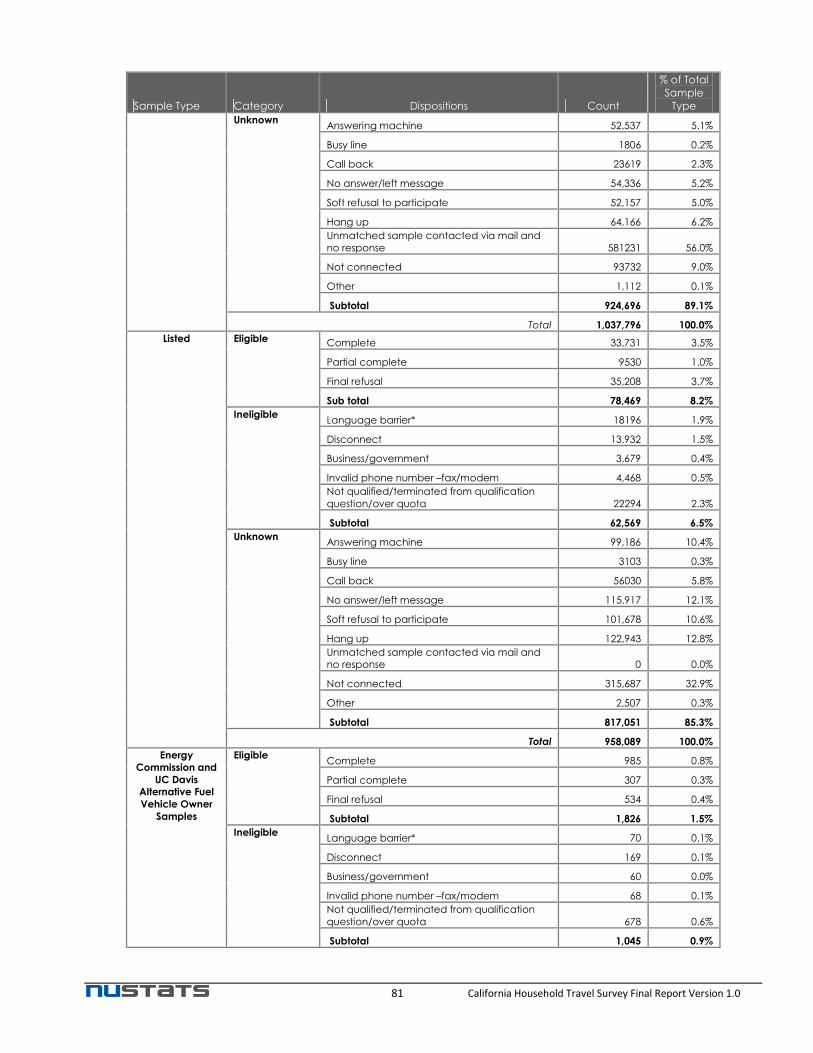
81 California Household Travel Survey Final Report Version 1.0
Sample Type Category Dispositions Count
% of Total
Sample
Type
Unknown Answering machine 52,537 5.1%
Busy line 1806 0.2%
Call back 23619 2.3%
No answer/left message 54,336 5.2%
Soft refusal to participate 52,157 5.0%
Hang up 64,166 6.2%
Unmatched sample contacted via mail and
no response 581231 56.0%
Not connected 93732 9.0%
Other 1,112 0.1%
Subtotal 924,696 89.1%
Total 1,037,796 100.0%
Listed Eligible Complete 33,731 3.5%
Partial complete 9530 1.0%
Final refusal 35,208 3.7%
Sub total 78,469 8.2%
Ineligible Language barrier* 18196 1.9%
Disconnect 13,932 1.5%
Business/government 3,679 0.4%
Invalid phone number –fax/modem 4,468 0.5%
Not qualified/terminated from qualification
question/over quota 22294 2.3%
Subtotal 62,569 6.5%
Unknown Answering machine 99,186 10.4%
Busy line 3103 0.3%
Call back 56030 5.8%
No answer/left message 115,917 12.1%
Soft refusal to participate 101,678 10.6%
Hang up 122,943 12.8%
Unmatched sample contacted via mail and no response 0 0.0%
Not connected 315,687 32.9%
Other 2,507 0.3%
Subtotal 817,051 85.3%
Total 958,089 100.0%
Energy
Commission and
UC Davis
Alternative Fuel
Vehicle Owner
Samples
Eligible Complete 985 0.8%
Partial complete 307 0.3%
Final refusal 534 0.4%
Subtotal 1,826 1.5%
Ineligible Language barrier* 70 0.1%
Disconnect 169 0.1%
Business/government 60 0.0%
Invalid phone number –fax/modem 68 0.1%
Not qualified/terminated from qualification
question/over quota 678 0.6%
Subtotal 1,045 0.9%

82 California Household Travel Survey Final Report Version 1.0
Sample Type Category Dispositions Count
% of Total
Sample
Type
Unknown Answering machine 1,122 0.9%
Busy line 19 0.0%
Call back 886 0.7%
No answer/left message 1,241 1.0%
Soft refusal to participate 2,198 1.8%
Hang up 1,437 1.2%
Unmatched sample contacted via mail and
no response 111343 91.4%
Not connected 627 0.5%
Other 91 0.1%
Subtotal 118,964 97.6%
Total 121,835 100.0%
Kern County
Transit Intercept
Sample
Eligible Complete 443 14.8%
Partial complete 28 0.9%
Final refusal 135 4.5%
Subtotal 606 20.2%
Ineligible Language barrier* 7 0.2%
Disconnect 289 9.6%
Business/government 11 0.4%
Invalid phone number –fax/modem 5 0.2%
Not qualified/terminated from qualification
question/over quota 13 0.4%
Subtotal 325 10.8%
Unknown Answering machine 164 5.5%
Busy line 1 0.0%
Call back 29 1.0%
No answer/left message 60 2.0%
Soft refusal to participate 99 3.3%
Hang up 106 3.5%
Not contacted (No contact info) 1598 53.3%
Not connected 11 0.4%
Other 1 0.0%
Subtotal 2,069 69.0%
Total 3,000 100.0%
*Language barrier refers to a language other than English or Spanish.
6.4.2 CASRO Response Rate
Using the CASRO response rate calculation, which takes into account ineligible sample and call outcome
unknown sample, the CHTS main survey had a recruit response rate of 4.9%. This is in line with other household
surveys that report CASRO rates. However, the main survey CASRO response rate is lower than the CHTS pretest
CASRO response rate of 5.6%. This most likely reflects the larger size of the main CHTS survey. Overall retrieval
rate was 67.3%.

83 California Household Travel Survey Final Report Version 1.0
6.4.3 Simple Response Rate
For purposes of comparison of recruitment and retrieval rates by sample type and by geography, the simple
response rate calculations are presented. Recruitment rates and response rates by sample type are shown in
Table 6.4.3. As is frequently seen in household travel surveys, the ABS Unmatched sample resulted in the lowest
response rate (0.4%) as compared with other sample types. Since there was no telephone number associated
with the household, these households would have had to self-recruit online. The next lowest response rate was
for the Energy Commission's sample of alternative fuel vehicle owners (0.6%).
Table 6.4.3: Recruitment Rates and Response Rates by Sample Type
Sample
Type
Specific
Sample Type
Sampled
HH
Recruited
HH
Recruitment
Rate
Retrieved
HH
Retrieval
Rate
Response
Rate
(A) (B) (B)/(A) (C) (C)/(B) (C)/(A)
Address–
based sample
ABS Matched 452,276 24,926 5.5% 16,774 67.3% 3.7%
ABS Unmatched 585,520 2,996 0.5% 2,458 82.0% 0.4%
Listed RDD
sample
Listed General 444,066 13,782 3.1% 9,489 68.9% 2.1%
Targeted Hispanic Surname
106,338 3,085 2.9% 1,722 55.8% 1.6%
Targeted Low
Income Household (<25K)
80,552 2,861 3.6% 1,757 61.4% 2.2%
Targeted Young
Household
(Age<25)
61,517 2,224 3.6% 1,325 59.6% 2.2%
Targeted Large Household
(HHSIZ>3)
156,046 7,461 4.8% 5,036 67.5% 3.2%
Listed Household From Transit
Oversampling
Area
62,782 2,589 4.1% 1,713 66.2% 2.7%
Listed Household From Zero Vehicle
Household
46,788 1,730 3.7% 1,118 64.6% 2.4%
Non–
probability
samples
Energy
Commission Database of
Alternative Fuel
Vehicle Owners
121,021 873 0.7% 707 81.0% 0.6%
Kern County Transit Intercept
Sample
3,000 443 14.8% 230 51.9% 7.7%
UC Davis Sample of Alternative Fuel
Vehicle Owners
814 112 13.8% 102 91.1% 12.5%
Total 2,120,720 63,082 3.0% 42,431 67.3% 2.0%
Table 6.4.4 presents the recruitment rate and response rate by each of the 30 sampling strata for the Address-
based (ABS) sample. Humboldt County had the highest response rate (4.5%), while two strata in the SCAG region
had the lowest response rates (1.4 and 1.5).

84 California Household Travel Survey Final Report Version 1.0
Table 6.4.4: Recruitment Rates and Response Rates by 30 Sampling Strata for ABS Sample
Sampling
Strata
MPO/
STRATA
Sampled
HH
Recruited
HH
Recruitment
Rate
Retrieved
HH
Retrieval
Rate
Response
Rate
(A) (B) (B)/(A) (C) (C)/(B) (C)/(A)
1
SCAG
25,424 775 3.0% 481 62.1% 1.9%
2 160,208 3,464 2.2% 2,401 69.3% 1.5%
3
654,423 14,688 2.2% 9,430 64.2% 1.4% 3
4
178,269 5,368 3.0% 3,404 63.4% 1.9% 4
5
MTC
60,352 2,341 3.9% 1,700 72.6% 2.8%
6 56,319 1,949 3.5% 1,389 71.3% 2.5%
7 16,863 617 3.7% 461 74.7% 2.7%
8 28,506 1,207 4.2% 870 72.1% 3.1%
9 15,145 496 3.3% 317 63.9% 2.1%
10 28,639 905 3.2% 628 69.4% 2.2%
11 44,580 1,460 3.3% 1,076 73.7% 2.4%
12 47,952 1,588 3.3% 1,142 71.9% 2.4%
13 75,150 2,917 3.9% 2,136 73.2% 2.8%
14 SANDAG 81,672 2,437 3.0% 1,689 69.3% 2.1%
15 SACOG 79,296 2,693 3.4% 2,038 75.7% 2.6%
16 Nevada 7,763 269 3.5% 188 69.9% 2.4%
17 Lassen
10,646 491 4.6% 361 73.5% 3.4%
17 Plumas
17 Sierra
18 Modoc
11,696 689 5.9% 499 72.4% 4.3%
18 Siskiyou
18 Trinity
19 Del Norte 4,582 266 5.8% 189 71.1% 4.1%
20 Humboldt 7,182 399 5.6% 321 80.5% 4.5%
21 Lake
12,367 557 4.5% 357 64.1% 2.9% 21 Mendocino
22 Fresno
182,635 6,499 3.6% 4,062 62.5% 2.2%
22 Kern
22 Kings
22 Madera
22 Tulare
23
AMBAG
79,784 2,768 3.5% 1,964 71.0% 2.5%
23
23
24 Merced
82,687 2,517 3.0% 1,656 65.8% 2.0%
24 San Joaquin
24 Stanislaus
25
San Luis
Obispo 60,457 1,846 3.1% 1,282 69.4% 2.1%

85 California Household Travel Survey Final Report Version 1.0
Sampling
Strata
MPO/
STRATA
Sampled
HH
Recruited
HH
Recruitment
Rate
Retrieved
HH
Retrieval
Rate
Response
Rate
(A) (B) (B)/(A) (C) (C)/(B) (C)/(A)
25
Santa
Barbara
26 Butte
24,182 1,126 4.7% 786 69.8% 3.3%
26 Shasta
26 Tehama
27 Colusa
10,805 432 4.0% 289 66.9% 2.7% 27 Glenn
28 TMPO
11,432 405 3.5% 299 73.8% 2.6% 28 TMPO
29 Alpine
22,654 1,032 4.6% 720 69.8% 3.2%
29 Amador
29 Calaveras
29 Mariposa
29 Tuolumne
30 Inyo
7,905 406 5.1% 296 72.9% 3.7% 30 Mono
Unknown 31,145 475 1.5% 0 0.0% 0.0%
Total 2,120,720 63,082 3.0% 42,431 67.3% 2.0%

86 California Household Travel Survey Final Report Version 1.0
7.0 Survey Data Weighting and Expansion
From a finite population sampling theory perspective, analytic weights are needed to develop estimates of
population parameters and, more generally, to draw inferences about the sampled population. Without the use
of analytic weights, population estimates are subject to biases of unknown (and possibly large) magnitude.
Consequently, analytic weights are crucial to obtain survey estimates with minimal bias.
The weighting approach utilized in this study accounts for the biases associated with sampling and robustness of
the data collected. Specifically, the components of the analytic weights generated from method are as follows:
• Sampling weights
• Raking adjustment
Analytic weights are computed at the household and person levels. These weights adjust the relative importance
of responses to reflect the different probabilities of selection by respondents, and align the sample distributions
to population distributions. This section discusses the components of the household weight and person weight in
detail.
7.1 Household Weight
7.1.1 Sampling Weight
The sampling weight reflects the probability of selection of a telephone number or an address from the sampling
frame. Considering the dual-sampling frame employed in this study, separate sampling weights are calculated for
samples from the listed residential sampling frame and those from the address-based sampling frame. Sample
orders were occurred in several waves. As sampling frame gets updated frequently, sample universe continued
to be changed whenever sample were drawn. Therefore, sampling weights were calculated for each sample
order. Specifically, the sampling weight for a sampling unit j in the sampling frame (denoted as ,j SampFrW ) from
each sample draw, is simply the reciprocal of the selection probability of the sampling unit.
,
,
1
Probj SampFr
j SampFr
W =
Where:
The sampling unit j is a landline residential phone number in the listed residential frame or an address in the
address-based sampling frame.
Sampling frame SampFr is listed residential sampling frame or address-based sampling frame.
The sampling weights help adjust for oversampling of specific geographies or demographic groups of interest for
which we had implemented controls to ensure adequate observations in these groups. To illustrate, the sampling
weight associated with an address-based sample is simply computed as the number of addresses (universe) in
the address-based frame divided by number of sample pieces ordered from the frame for the study area for each
sample order. For this study, samples (i.e. addresses) was drawn by county for CHTS, except TMPO where
samples were drawn from the census tracts within the MPO area(see the list of census tracts in Appendix Q)
from address-based sampling frame, sampling weights will be computed by county except TMPO for the samples
drawn from the address-based sampling frame. Samples (i.e. residential land line phone) were also drawn from

87 California Household Travel Survey Final Report Version 1.0
the listed sampling frame. The listed sample was divided evenly among six targeted groups including: Hispanic
surnames, low income households with annual income less than $25,000, young households with all members
aged 25 or younger, large households with 4 or more persons, transit oversample, zero-vehicle household.
Sampling weights were computed separately for samples drawn from each of the six targeted sampling groups. It
is important to note that samples from four of the targeted listed sampling groups – (Hispanic surnames, low
income households with annual income less than $25,000, young households with all members aged 25 or
younger, and large households with 4 or more persons) were drawn across the state, while samples from transit
oversample or zero-vehicle household sampling groups were drawn from the targeted census tracts Zero-vehicle
household census statistics were available from the 2005-2009 ACS 5-year estimate data at the 2000 census tract
level (see the list of 2010 and 2000 census tracts in Appendix Q) when the sampling plan was designed.
Exclusion of Samples from Non–probability Sampling Frame
In CHTS, three other non–sampling methodologies were implemented in order to capture certain population of
the interest: Energy Commission samples were drawn from two sources – 2009 database from the Department
of Motor Vehicles (DMV), vehicle owner database from University of California at Davis and intercept sample for
Kern County transit users. These non-probability based samples were assigned with the base sampling weight of
1 and included in the next step of raking procedure.
7.1.2 Raking Adjustment
Raking improves the reliability of survey estimates; hence, a raking adjustment was used to align the weighted
sample with population statistics from the latest available census data - 2011 American Community Survey (ACS)
1-year estimates or 2007-2011 5-year estimates, depending on selected raking control variables and base-
geography. In particular, the aforementioned weights were adjusted so that the sums of the adjusted weights
are equal to known population totals for certain subgroups of the population, defined by demographic
characteristics and geographic variables. Variables and variable categories used for raking at the household level
are as follows:
• Household size (1, 2, 3, 4 or more) – State-wide distribution
• Household income (Less than $24,999, $25,000 – $49,999, $50,000 - $74,999, $75,000-$99,999,
$100,000-$149,999, $150,000 or above) – State-wide distribution
• Total number of workers in the household (0, 1, 2, 3 or more) – State-wide distribution
• Total number of vehicles in the household (0, 1, 2, 3 or more) – State-wide distribution
• County of Residence – by County
• These variables were chosen as raking variables due to significant differences in coverage by categories
of these variables. Therefore, it is reasonable to expect that maximum bias reduction would be achieved
using these variables. It is important to note that the missing values in the raking variables were imputed
to calculate the raking adjustments using the well-known hot deck method, in which a missing value is
imputed using the data from other observations in the same dataset. Missing income was imputed
before the household level raking procedure using a mean of household income for combination of OWN
(home ownership), HHSIZ (household size) and HHVEH (number of household vehicles) variables. A mean
of each combination was calculated and applied to the refused income values for the relevant category.
• The raking procedure was based on an iterative proportional fitting procedure, and involves
simultaneous ratio adjustments to two or more marginal distributions of population counts. The raking
procedure was performed in a sequence of adjustments. First, base weights (sampling weights) were

88 California Household Travel Survey Final Report Version 1.0
adjusted to one marginal distribution and then to the second marginal distribution, and so on. One
sequence of adjustments to the marginal distributions was known as a cycle or iteration. The procedure
was repeated until convergence was achieved.
• Note that state-wide marginal control total data were obtained from 2011 ACS 1-year estimates while
county of residence data were obtained from 2007-2011 ACS 5-year estimates due to small counties
where data are not available from 1-year or 3-year estimates.
• Following the raking procedure, inordinately large weights, a by-product of raking, ought to be capped in
order to prevent samples with extremely large weight from skewing other variables that are not
controlled by the weighting process and travel pattern. There were no “very large” weights exceeding a
maximum of five times the mean weight observed after the household level raking procedure, so capping
was not necessary.
Table 7.1.2.1 shows the survey and population distributions by demographic and geographic raking variables
for the study area. A comparison of the unweighted distribution and the weighted distribution of these
raking variables indicates that the raking procedure has aligned the sample statistics to the population
statistics.
Table 7.1.2.1: Raking Adjustment at Household Level
Key variables Unweighted Weighted ACS 2011 1 year
Difference
(% points)
Weighted-
ACS
Household Size
1 9140 21.5% 10379 24.5% 3050172 24.5% 0.0%
2 16319 38.5% 12744 30.0% 3745136 30.0% 0.0%
3 6821 16.1% 6939 16.4% 2039065 16.4% 0.0%
4 or more 10151 23.9% 12368 29.2% 3634370 29.2% 0.0%
Total 42431 100.0% 42431 100.0% 12468743 100.0% 0.0%
Income*
Less than $24999 6431 16.58% 8544 21.83% 2764797 22.17% -0.34%
$25000 – $49999 7923 20.43% 9370 23.94% 2759357 22.13% 1.81%
$50000 - $74999 6903 17.80% 6204 15.85% 2112377 16.94% -1.09%
$75000-$99999 5870 15.13% 5017 12.82% 1488173 11.94% 0.88%
$100000-$149999 6470 16.68% 4659 11.90% 1768081 14.18% -2.28%
$150000 or above 5192 13.39% 5344 13.65% 1575958 12.64% 1.01%
Total 38789 100.00% 39138 100.00% 12468743 100.00% 0.00%
Number of Household Vehicles
0 2459 5.8% 3402 8.0% 999,638 8.0% 0.0%
1 12678 29.9% 13886 32.7% 4,080,664 32.7% 0.0%
2 18657 44.0% 15788 37.2% 4,639,481 37.2% 0.0%
3 or more 8637 20.4% 9355 22.1% 2,748,960 22.1% 0.0%
Total 42431 100.0% 42431 100.0% 12468743 100.0% 0.0%
Number of Household Workers

89 California Household Travel Survey Final Report Version 1.0
Key variables Unweighted Weighted ACS 2011 1 year
Difference
(% points)
Weighted-
ACS
0 9120 21.5% 10809 25.5% 3175985 25.5% 0.0%
1 17915 42.2% 16894 39.8% 4964467 39.8% 0.0%
2 12818 30.2% 11527 27.2% 3387597 27.2% 0.0%
3 or more 2578 6.1% 3201 7.5% 940694 7.5% 0.0%
Total 42431 100.0% 42431 100.0% 12468743 100.0% 0.0%
Household Counts by County
Alameda 1700 4.0% 1830 4.3% 536160 4.3% 0.0%
Alpine 21 0.1% 1 0.0% 357 0.0% 0.0%
Amador 182 0.4% 49 0.1% 14283 0.1% 0.0%
Butte 360 0.9% 291 0.7% 85219 0.7% 0.0%
Calaveras 176 0.4% 64 0.2% 18865 0.2% 0.0%
Colusa 107 0.3% 24 0.1% 6989 0.1% 0.0%
Contra Costa 1389 3.3% 1266 3.0% 370925 3.0% 0.0%
Del Norte 189 0.5% 34 0.1% 9818 0.1% 0.0%
El Dorado 412 1.0% 235 0.6% 68812 0.6% 0.0%
Fresno 1115 2.6% 974 2.3% 285338 2.3% 0.0%
Glenn 182 0.4% 32 0.1% 9483 0.1% 0.0%
Humboldt 321 0.8% 183 0.4% 53724 0.4% 0.0%
Imperial 481 1.1% 164 0.4% 48117 0.4% 0.0%
Inyo 189 0.5% 27 0.1% 7910 0.1% 0.0%
Kern 1544 3.6% 857 2.0% 250999 2.0% 0.0%
Kings 293 0.7% 139 0.3% 40716 0.3% 0.0%
Lake 182 0.4% 88 0.2% 25654 0.2% 0.0%
Lassen 152 0.4% 34 0.1% 10097 0.1% 0.0%
Los Angeles 8219 19.4% 10984 25.9% 3218518 25.9% 0.0%
Madera 311 0.7% 143 0.3% 42032 0.3% 0.0%
Marin 461 1.1% 351 0.8% 102832 0.8% 0.0%
Mariposa 148 0.4% 26 0.1% 7607 0.1% 0.0%
Mendocino 175 0.4% 116 0.3% 34102 0.3% 0.0%
Merced 474 1.1% 253 0.6% 74079 0.6% 0.0%
Modoc 111 0.3% 13 0.0% 3947 0.0% 0.0%
Mono 107 0.3% 18 0.0% 5416 0.0% 0.0%
Monterey 1022 2.4% 427 1.0% 125217 1.0% 0.0%
Napa 317 0.8% 169 0.4% 49640 0.4% 0.0%
Nevada 188 0.4% 142 0.3% 41561 0.3% 0.0%
Orange 2401 5.7% 3369 7.9% 987164 7.9% 0.0%

90 California Household Travel Survey Final Report Version 1.0
Key variables Unweighted Weighted ACS 2011 1 year
Difference
(% points)
Weighted-
ACS
Placer 481 1.1% 446 1.1% 130736 1.1% 0.0%
Plumas 150 0.4% 32 0.1% 9434 0.1% 0.0%
Riverside 1701 4.0% 2296 5.4% 672896 5.4% 0.0%
Sacramento 825 1.9% 1744 4.1% 510976 4.1% 0.0%
San Benito 268 0.6% 57 0.1% 16785 0.1% 0.0%
San Bernardino 1703 4.0% 2044 4.8% 598822 4.8% 0.0%
San Diego 1689 4.0% 3631 8.6% 1064048 8.6% 0.0%
San Francisco 1076 2.5% 1155 2.7% 338366 2.7% 0.0%
San Joaquin 630 1.5% 727 1.7% 212902 1.7% 0.0%
San Luis Obispo 847 2.0% 348 0.8% 101993 0.8% 0.0%
San Mateo 1142 2.7% 875 2.1% 256423 2.1% 0.0%
Santa Barbara 435 1.0% 483 1.1% 141635 1.1% 0.0%
Santa Clara 2136 5.0% 2047 4.8% 599652 4.8% 0.0%
Santa Cruz 674 1.6% 320 0.8% 93834 0.8% 0.0%
Shasta 250 0.6% 236 0.6% 69147 0.6% 0.0%
Sierra 59 0.1% 5 0.0% 1328 0.0% 0.0%
Siskiyou 212 0.5% 67 0.2% 19782 0.2% 0.0%
Solano 628 1.5% 475 1.1% 139312 1.1% 0.0%
Sonoma 870 2.1% 629 1.5% 184170 1.5% 0.0%
Stanislaus 552 1.3% 563 1.3% 164933 1.3% 0.0%
Sutter 168 0.4% 108 0.3% 31668 0.3% 0.0%
Tehama 176 0.4% 81 0.2% 23810 0.2% 0.0%
Trinity 176 0.4% 20 0.1% 5731 0.1% 0.0%
Tulare 799 1.9% 438 1.0% 128324 1.0% 0.0%
Tuolumne 193 0.5% 76 0.2% 22157 0.2% 0.0%
Ventura 1211 2.9% 904 2.1% 264982 2.1% 0.0%
Yolo 246 0.6% 238 0.6% 69860 0.6% 0.0%
Yuba 205 0.5% 82 0.2% 23885 0.2% 0.0%
Total 42431 100.0% 42431 100.0% 12433172 100.0% 0.0%
*The weighted survey data distribution for household income uses unimputed value and excludes the refusals.
7.1.3 Final Expanded Household Weight
The final analytic weight is simply the product of sampling weight and raking adjustment. Following the
computation of this weight, an expansion procedure was undertaken to get the final ‘expanded’ analytic weight
so that the weighted survey dataset can provide estimates for the total population in the study area. The
expansion process simply takes the weighted total number of households and multiplies each household by a
factor that, when applied, expands the data to represent the universe of households in the study area of State of

91 California Household Travel Survey Final Report Version 1.0
California. The 2011 ACS 1-year estimate was used to get the total household counts in the state of California. To
derive the expansion factor, a simple division was used: Expansion Factor = N(Universe)/N(Surveyed. This
translates to a survey universe of 12,433,172 households.
The final expanded household weight was appended to the Household and Vehicle data files.
7.2 Person Weight
Person weight is a product of the final household weight and the person level raking weight. Person data
weighted by “final household weight” was raked to align it to population statistics from the 2011 ACS 1-year
estimates except population counts by county, which was pulled from 2007-2011 ACS 5-year estimates. Variables
used for raking at the person level are as follows:
• Hispanic Status (Hispanic, Non-Hispanic) – State-wide distribution.
• Ethnicity (White, African American, Asian, Other) – State-wide distribution.
• Age (less than 20 years, 20 –34 years, 35 – 54 years, 55 – 64 years, 65 years or older) – State-wide
distribution.
• Employment Status (Part-time or full-time Employed, Not-employed) – State-wide distribution.
• County of Residence (Three smallest counties- Alpine, Amador and Calaveras) were grouped due to
difficulty of convergence by small sample size) – by County
Before the raking procedure, any missing data for Hispanic status/race or age were imputed using hot–deck
imputation method which is the most commonly used method for missing data imputation. With this method, a
missing value is imputed from randomly selected similar records. To select similar records, other reference
demographic variables known to have a strong correlation with the imputing variable are used to compute mean
or mode – a statistical term for the number that appears most often – to replace missing value. Imputation of
these variables was carried out as follows:
• Hispanic status/race is a categorical variable. Hence, mode (a statistical term meaning the value that
appears most often) was calculated and applied for missing value. For race, mode by household income
category was computed and applied to race refusal records in the same household income category. For
Hispanic status, mode of Hispanic status by combination of household income and race was computed
and applied to missing or refusal values of the same household income and age group.
• Age is a scale variable. Hence, mean age for combination of education level, work status, and student
status was computed and applied to age refusals. If education level was refused or missing, a mean age
of relevant work status and student status category was applied. If all the variables used for imputation
are refusals, and the overall average age was applied.
Following the raking procedure, any very large weights were capped to equal a maximum of five times the mean
weight. Table 7.2.1 shows the survey and population distribution by the aforementioned raking variables.

92 California Household Travel Survey Final Report Version 1.0
Table 7.2.1: Survey and Population Distribution by Raking Variables
Key variables Unweighted Weighted ACS 2011 1 year
Difference
(% points)
Weighted-ACS
Hispanic Status
Hispanic 27692 25.7% 39154 36.5% 14359500 38.1% -1.56%
Non-Hispanic 80267 74.3% 67995 63.5% 23332412 61.9% 1.56%
Total 107959 100.0% 107149 100.0% 37691912 100.0% 0.00%
Age
less than 20 years 24170 23.0% 28108 26.7% 9,873,223 26.2% 0.55%
20 – 34 years 12163 11.6% 21414 20.4% 7,866,957 20.9% -0.49%
35 – 54 years 29175 27.7% 27008 25.7% 9,913,281 26.3% -0.60%
55 – 64 years 21985 20.9% 11249 10.7% 4,011,905 10.6% 0.06%
65 years or older 17696 16.8% 17305 16.5% 6,026,546 16.0% 0.48%
Total 105189 100.0% 105084 100.0% 37691912 100.0% 0.00%
Race
White 74882 70.5% 65088 61.8% 23698393 62.9% -1.05%
Black or African American 3356 3.2% 6403 6.1% 2253905 6.0% 0.10%
American Indian or Alaska
Native
5573 5.2% 848 0.8% 289597 0.8% 0.04%
Asian 6564 6.2% 14054 13.3% 4970627 13.2% 0.16%
OTHER 15866 14.9% 18889 17.9% 6479390 17.2% 0.75%
Total 106241 100.0% 105282 100.0% 37691912 100.0% 0.00%
Employment Status
Yes 51838 47.6% 46502 42.8% 16047067 42.6% 0.20%
No 57027 52.4% 62216 57.2% 21644845 57.4% -0.20%
Total 108865 100.0% 108718 100.0% 37691912 100.0% 0.00%
Population by County
Alameda 4191 3.8% 4443 4.1% 1494876 4.0% 0.03%
Alpine 56 0.1% 3 0.0% 1167 0.0% 0.00%
Amador 373 0.3% 103 0.1% 38244 0.1% -0.01%
Butte 853 0.8% 655 0.6% 219309 0.6% 0.01%
Calaveras 372 0.3% 149 0.1% 45794 0.1% 0.01%
Colusa 248 0.2% 63 0.1% 21297 0.1% 0.00%
Contra Costa 3490 3.2% 3100 2.8% 1037817 2.8% 0.03%
Del Norte 458 0.4% 85 0.1% 28561 0.1% 0.00%
El Dorado 975 0.9% 535 0.5% 179878 0.5% 0.00%
Fresno 3016 2.8% 2662 2.4% 920623 2.5% -0.05%
Glenn 455 0.4% 84 0.1% 28027 0.1% 0.00%
Humboldt 740 0.7% 399 0.4% 133585 0.4% 0.00%
Imperial 1439 1.3% 511 0.5% 171343 0.5% 0.00%

93 California Household Travel Survey Final Report Version 1.0
Key variables Unweighted Weighted ACS 2011 1 year
Difference
(% points)
Weighted-ACS
Inyo 431 0.4% 55 0.1% 18457 0.0% 0.00%
Kern 4096 3.8% 2458 2.3% 829254 2.2% 0.01%
Kings 833 0.8% 455 0.4% 152335 0.4% 0.00%
Lake 384 0.4% 192 0.2% 64392 0.2% 0.00%
Lassen 339 0.3% 105 0.1% 35001 0.1% 0.00%
Los Angeles 21184 19.4% 29068 26.6% 9787747 26.5% 0.16%
Madera 860 0.8% 443 0.4% 149611 0.4% 0.00%
Marin 1062 1.0% 739 0.7% 250666 0.7% 0.00%
Mariposa 324 0.3% 55 0.1% 18290 0.0% 0.00%
Mendocino 418 0.4% 261 0.2% 87525 0.2% 0.00%
Merced 1327 1.2% 748 0.7% 253606 0.7% 0.00%
Modoc 254 0.2% 29 0.0% 9587 0.0% 0.00%
Mono 262 0.2% 42 0.0% 14016 0.0% 0.00%
Monterey 2573 2.4% 1203 1.1% 411385 1.1% -0.01%
Napa 763 0.7% 385 0.4% 135377 0.4% -0.01%
Nevada 431 0.4% 294 0.3% 98392 0.3% 0.00%
Orange 6357 5.8% 8838 8.1% 2989948 8.1% 0.01%
Placer 1166 1.1% 1016 0.9% 343554 0.9% 0.00%
Plumas 333 0.3% 60 0.1% 20192 0.1% 0.00%
Riverside 4920 4.5% 6394 5.9% 2154844 5.8% 0.03%
Sacramento 2151 2.0% 3970 3.6% 1408480 3.8% -0.17%
San Benito 726 0.7% 164 0.2% 54873 0.1% 0.00%
San Bernardino 4882 4.5% 6025 5.5% 2023452 5.5% 0.05%
San Diego 4606 4.2% 8779 8.0% 3060849 8.3% -0.23%
San Francisco 2249 2.1% 2379 2.2% 797983 2.2% 0.02%
San Joaquin 1717 1.6% 2013 1.8% 680277 1.8% 0.01%
San Luis Obispo 1900 1.7% 797 0.7% 267871 0.7% 0.01%
San Mateo 2801 2.6% 2126 1.9% 711622 1.9% 0.02%
Santa Barbara 1046 1.0% 1203 1.1% 419793 1.1% -0.03%
Santa Clara 5868 5.4% 5261 4.8% 1762754 4.8% 0.05%
Santa Cruz 1571 1.4% 775 0.7% 259402 0.7% 0.01%
Shasta 589 0.5% 529 0.5% 177231 0.5% 0.01%
Sierra 120 0.1% 10 0.0% 3277 0.0% 0.00%
Siskiyou 472 0.4% 133 0.1% 44687 0.1% 0.00%
Solano 1575 1.4% 1213 1.1% 411620 1.1% 0.00%
Sonoma 2031 1.9% 1429 1.3% 478551 1.3% 0.02%
Stanislaus 1540 1.4% 1522 1.4% 512469 1.4% 0.01%

94 California Household Travel Survey Final Report Version 1.0
Key variables Unweighted Weighted ACS 2011 1 year
Difference
(% points)
Weighted-ACS
Sutter 411 0.4% 281 0.3% 94192 0.3% 0.00%
Tehama 438 0.4% 188 0.2% 62985 0.2% 0.00%
Trinity 381 0.3% 41 0.0% 13711 0.0% 0.00%
Tulare 2186 2.0% 1298 1.2% 436234 1.2% 0.01%
Tuolumne 419 0.4% 166 0.2% 55736 0.2% 0.00%
Ventura 3343 3.1% 2371 2.2% 815745 2.2% -0.03%
Yolo 616 0.6% 594 0.5% 198889 0.5% 0.01%
Yuba 492 0.5% 212 0.2% 71817 0.2% 0.00%
Total 109113 100.0% 109113 100.0% 36969200 100.0% 0.00%
7.2.1 Final Expanded Person Weight
Following computation of “final person weight”, weights were then expanded to reflect the total 36,969,200
persons residing in the State of California. The final expanded person weight was appended to Person, Place and
Activity data files.
7.3 GPS Trip Correction Factors
In a household travel survey, accuracy of the reported trips is as important as the coverage of survey samples
within the survey universe. Unfortunately, misreporting of travel behaviors occur due to honest mistakes, privacy
concerns, nonchalance, and other factors (Zmud, 2003). Advances in global positioning systems (GPS) have made
it a feasible and affordable technology for collecting more reliable travel behavior information, in a passive way
and with higher accuracy. In the California Household Travel Survey (CHTS), final overall sample size covers non-
GPS households and GPS-enabled households. Even though GPS households only occupy 12% of the total
samples, general misreporting patterns and trip correction factors can be identified through comparing the trips
of households recorded passively by vehicle-mounted/Wearable GPS devices and the corresponding trips
recorded actively by members in the same households via other approaches (e.g. travel diaries and computer-
assisted telephone interviewing CATI). Applying trip correction factors to non-GPS household trips significantly
improves overall survey accuracy. In this study, the trip correction process was conducted in three steps:
• Initial analysis on misreporting/over-reporting trips
• Identifying the key factors (trip characteristics or demographic characteristics of households/persons)
that would significantly impact the misreporting or over-reporting rate through descriptive statistics and
ANOVA analysis
• Creating trip correction factors through logistic regression analysis for each groups of trips with different
characteristics defined by the key factors
7.3.1 Initial Trip Matching Analysis
GeoStats conducted the initial trip match analysis by comparing the sample GPS-identified trips and the sample
diary-recorded trips. This analysis isolated three types of trips:
• Matched trip (M) – trips that were found in both the sample GPS trip table and the sample diary trip
table

95 California Household Travel Survey Final Report Version 1.0
• Underestimated trip (U) – trips that were found in the sample GPS trip table but not in the sample diary
trip table
• Overestimated trip (O) – trips that were found in the sample diary trip table but not in the sample
GPS/OBD trip table
For example, if a non-stop trip starting at home and ending at work was not only identified from the
respondent’s GPS traces but also recorded in his/her diary, this trip is labeled as a matched trip; if the GPS traces
revealed that the respondent stopped at a gas station along his/her way to work but his/her diary-recorded a
home to work trip, the GPS trip from home to gas station and the GPS trip from gas station to work would be
identified as two underestimated trips because they did occur but not recorded in the diary, while the home to
work trip would be labeled as an overestimated trip in the diary. Table 7.3.1.1 gives a summary of the three types
of trips in the sample.
Table 7.3.1.1: Distribution of Trips of Different Match Types
MATCH TYPE Frequency Percent
Cumulative
Frequency
Cumulative
Percent
Overestimated Trip 4,218 5.2% 4,218 5.2%
Matched Trip 63,672 78.3% 67,890 83.5%
Underestimated Trip 13,399 16.5% 81,289 100.0%
Matched trips (63,672) and underestimated trips (13,399) are trips that really occurred (Real Trips), while the
overestimated trips did not really occur (Unreal Trips) but were recorded in the diary by mistake. Trips recorded
in diaries consist of matched trips (63,672) and overestimated trips (4,218). The diary-recorded trips
(67,890=63,672+4,218) are the base upon which trip correction factors would apply since 88% of respondents in
this survey who filled out their diaries without GPS/OBD devices installed on their vehicles. Among diary-
recorded trips, around 5.2% are the overestimated trips which need to be corrected down. At the same time,
diary-recorded trips need to be corrected up to compensate the 16.5% underestimated trips. Table 7.3.1.2
presents an initial estimate of the total trip correction factor to explain how these data would be used to
perform trip correction in two steps.
Table 7.3.1.2: Distribution of Trips of Different Match Types
TRIP
Overestimated
(964 Trips)
Matched
(15,500 Trips)
Underestimated
(2,967 Trips) Sum
Diary-recorded Trips x x
67,890
Real Trips
x x 77,071
Trip Correction Factor
=(Number of Real Trips) / (Number of Diary-recorded Trips)
= (M+U)/(M+O) =1.135
Corrected Trips =(Diary-recorded Trips)*(Trip Correction Factor)=67,890*1.135=77,071
The trip correction factor 1.135 in Table 7.3.1.2 is the average trip correction for all the diary-recorded trips from
the GPS sample. However, it is not wise to apply a single trip correction factor on the total number of trips
because trip misreporting/over-reporting rates change significantly under different environments. The following

96 California Household Travel Survey Final Report Version 1.0
sections will present the procedure and results of identifying the key factors that would impact trip
misreporting/over-reporting rates significantly and creating trip correction factors under conditions defined by
the key factors.
7.3.2 Identification of Key Trip and Demographic Factors
All of the trip characteristics and household/person demographic information available have been considered as
potential factors that would impact trip misreporting/over-reporting rates. After several rounds of screening by
descriptive correlation analysis and ANOVA, the following variables have been identified as the key factors due to
their significant correlation with the trip match type (matched, overestimated, and underestimated):
• Trip Travel Time: the time between the respondent leaving the origin and arriving the destination of a
trip
• Minimum Dwelling Time: the minimum between the dwelling times of the respondent at the origin and
at the destination
• Education Level of the Respondent
• Person Number of Trips: number of trips made by a respondent during the survey time period
Table 7.3.2.1 shows all of the key factors’ value ranges, F statistics from one-way ANOVA analysis against trip
match type, and the P value of the F test. All of the P values indicate a significant correlation between the factors
with trip match type at a 99% confidence level. However, the characteristics of the trips themselves – trip travel
time and minimum dwelling time – show much higher F statistics with trip match types than the person
demographic factors, the education level of a respondent, and the number of trips made by him/her. This means
trip characteristics would dominate in explaining why a trip would be misreported or over-reported. Among all of
the factors, the minimum dwelling time of the respondent at the origin or destination played the most important
role in his or her view to decide whether or not a trip is important enough to be logged in diaries. For example, a
trip with a short stop at a gas station is easily ignored by the respondents no matter how long they spend at the
other end of the trip.
Table 7.3.2.1: Key Trip and Demographic Factors
VARIABLES Value Range F Statistics P value
Minimum Dwelling Time
< 10 mins
> 10 mins and < 20 mins
> 20 mins and < 30 mins
> 30 mins 1470.86 <.0001
Trip Travel Time
< 10 mins
> 10 mins and < 20 mins
> 20 mins and < 30 mins
> 30 mins 1159.15 <.0001
Person Number of Trips
<= 5 trips
> 5 trips 74.30 <.0001
Education Level of
Respondents
< High School
Undergraduate
Graduate 67.42 <.0001

97 California Household Travel Survey Final Report Version 1.0
A unique trip correction factor is applied to each group of trips defined by any combination of the key factors.
These trip correction factors are created automatically from a logistic regression analysis which models the logit
odd ratio of the probability of a diary-recorded trip being underestimated or overestimated over being matched
with GPS-identified trips, i.e.
�� � ����� = ��� �� +�����
���
Where:
Pi = Probability of not finding match in GPS-identified trips ( i = underestimated or
overestimated);
Pm = Probability of finding match in GPS-identified trips
Xj = Independent variable j ( j = travel time, dwelling time, education level, person
trips)
βj = Coefficient of Independent variable j ( j = travel time, dwelling time,
education level, person trips)
Two models were built – the “Overestimated Trip” model estimated the probability of a diary trip being
overestimated over finding its match in GPS trips, while the “Underestimated Trip” model predicted the
probability of a diary trip being underestimated over finding its match in GPS trips. Trip correction factors can be
easily computed from the modeling results following a similar procedure shown in Table 7.3.2.1 as follows:
� = �+��+� = � +�/�
� + �/� = 1 + ��/��1 + ��/��
Table 7.3.3.1 gives the estimates of the coefficients of logistic models and the hypothesis test whether or not
these coefficients are significantly different from zero. All of the key factors are significant enough to be retained
in the models at a 95% confidence level.
7.3.3 Summary
The following conclusions have been drawn based on the logistic regression analysis results in Table 7.3.3.1.
• The probability of a diary trip being underestimated increases with the decrease in its travel time and the
minimum dwelling time at the origin and destination. On the contrary, the trend of overestimated
probability goes in the opposite direction. This may indicate that trips with short travel time and dwelling
time are easier ignored by respondents.
• Both the underestimated and overestimated probabilities of a diary trip decrease with the increase in
the education level of the respondent. This may indicate that respondents with higher education levels
are more capable of and are more reliable in filling out the travel diary correctly.

98 California Household Travel Survey Final Report Version 1.0
• Both the underestimated and overestimated probabilities of a diary trip decrease with the increase in
the number of trips made by the respondent. It may be because the proportion of ignored trips becomes
less with the increase in the total number of trips made by a person.
Each trip in the final delivery dataset will be attached with a trip correction factor, variable named as “TCF”.
“TripCorrectedWeight” is a final trip weight which is an outcome of [TCF]*[PERWGT] (trip correction factor *
person level weight).
Table 7.3.3.1: Estimate of Coefficients of Logistic Models
Parameter Model Type Estimate
Wald
Chi-Square Pr > ChiSq
Intercept Overestimated Trip -4.2696 1112.7153 <.0001
traveltime 10to20mins Overestimated Trip 1.9753 259.1221 <.0001
traveltime 20to30mins Overestimated Trip 2.468 339.933 <.0001
traveltime >30mins Overestimated Trip 3.4279 793.6214 <.0001
minDuration 10to20mins Overestimated Trip 0.2424 4.3751 0.0365
minDuration 20to30mins Overestimated Trip 0.2502 3.0996 0.0783
minDuration >30mins Overestimated Trip -0.1057 1.6212 0.2029
educa Undergraduate Overestimated Trip -0.4181 25.7287 <.0001
educa Graduate Overestimated Trip -0.5934 45.3166 <.0001
ptrips >5 Overestimated Trip -0.0463 0.3998 0.5272
Intercept Underestimated Trip -0.0684 2.486 0.1149
traveltime 10to20mins Underestimated Trip -0.4413 56.2228 <.0001
traveltime 20to30mins Underestimated Trip -0.7042 51.3444 <.0001
traveltime >30mins Underestimated Trip -0.2614 8.9541 0.0028
minDuration 10to20mins Underestimated Trip -1.1506 244.3857 <.0001
minDuration 20to30mins Underestimated Trip -1.374 175.501 <.0001
minDuration >30mins Underestimated Trip -2.3931 1014.0271 <.0001
educa Undergraduate Underestimated Trip -0.3671 51.6509 <.0001
educa Graduate Underestimated Trip -0.5317 94.0688 <.0001
ptrips >5 Underestimated Trip -0.927 438.0132 <.0001

99 California Household Travel Survey Final Report Version 1.0
8.0 Statewide Survey Results
The chapter contains the summary tables for weighted and expanded data and is based on unlinked trips. The
results represent all households in the dataset, as discussed in the data expansion section of Chapter 6). To run
results by specific strata, MPO or county refer to Chapter 7 or the Data User’s Guide (Appendix P) on how to
select these subsets of households. Survey results were weighted by four weight factors – own/rent status by
vehicle availability, households by county distribution, household size and income. All trip-level results presented
in this section and throughout the main report are based on unlinked trips. Table 8.0.1 summarizes the
recruitment and retrieval, by sampling strata, for the CHTS.
Table 8.0.1: 30 Sampling Strata Table
County
30
Sampling
Strata
Goals
Recruit
Goal
Recruited
HH
% of
REC
goal
Retrieve
Goal
Retrieved
HH
(Primary
Complete
s)
% of
RET
goal
% of 30
Sampling
Strata
Goals
% of
Secondary*
+ Primary
Completes
30 SS Goals
SCAG Imperial 564 692 775 112% 450 481 107% 85% 137%
Orange 3,353 4,117 3,469 84% 2,676 2,359 88% 70% 103%
Los Angeles 12,580 15,445 14,676 95% 10,039 9,293 93% 74% 117%
Ventura
Riverside 4,192 5,146 5,395 105% 3,345 3,359 100% 80% 129%
San Bernardino
MTC Alameda 1,730 2,123 2,309 109% 1,380 1,660 120% 96% 133%
Contra Costa 1,243 1,526 1,952 128% 992 1361 137% 109% 157%
Marin 599 735 593 81% 478 454 95% 76% 99%
Sonoma 955 1,172 1,216 104% 762 858 113% 90% 127%
Napa 393 483 496 103% 314 315 100% 80% 126%
Solano 770 945 906 96% 614 624 102% 81% 118%
San Francisco 1,092 1,340 1,464 109% 871 1067 123% 98% 134%
San Mateo 1,204 1,477 1,590 108% 960 1117 116% 93% 132%
Santa Clara 1,911 2,346 2,933 125% 1,525 2,078 136% 109% 153%
SANDAG San Diego 2,177 2,672 2,453 92% 1,737 1,648 95% 76% 113%
SACOG El Dorado
2,889 3,546 2,902 82% 2,305 1,933 84% 67% 100%
Placer
Sacramento
Sutter
Yolo
Yuba
Nevada Nevada 328 403 263 65% 262 185 71% 56% 80%
Lassen Lassen
574 705 491 70% 458 360 79% 63% 86% Plumas Plumas
Sierra Sierra
Modoc Modoc
714 877 670 76% 570 499 88% 70% 94% Siskiyou Siskiyou
Trinity Trinity
Del Norte Del Norte 309 378 260 69% 246 188 76% 61% 84%

100 California Household Travel Survey Final Report Version 1.0
County
30
Sampling
Strata
Goals
Recruit
Goal
Recruited
HH
% of
REC
goal
Retrieve
Goal
Retrieved
HH
(Primary
Complete
s)
% of
RET
goal
% of 30
Sampling
Strata
Goals
% of
Secondary*
+ Primary
Completes
30 SS Goals
Humboldt Humboldt 416 511 398 78% 332 319 96% 77% 96%
Mendocino Mendocino 570 700 518 74% 455 351 77% 62% 91%
Lake Lake
Fresno Fresno
5,027 6,172 6,345 103% 4,012 4,046 101% 80% 126%
Kings Kings
Madera Madera
Kern Kern
Tulare Tulare
AMBAG Monterey
2,558 3,140 2,774 88% 2,041 1,945 95% 76% 108% Santa Cruz
San Benito
San Joaquin San Joaquin
2,169 2,663 2,521 95% 1,731 1,644 95% 76% 116% Stanislaus Stanislaus
Merced Merced
San Luis
Obispo
San Luis Obispo
1,282 1,574 1,852 118% 1,023 1,277 125% 100% 144% Santa
Barbara
Santa Barbara
Butte Butte
1,080 1,326 1,098 83% 862 778 90% 72% 102% Shasta Shasta
Tehama Tehama
Glenn Glenn 486 597 419 70% 388 289 74% 59% 86%
Colusa Colusa
TMPO (CA
part)
El Dorado 450 552 259 47% 359 299 83% 66% 58%
Placer
Alpine Alpine
1,003 1,232 974 79% 801 716 89% 71% 97%
Amador Amador
Calaveras Calaveras
Mariposa Mariposa
Tuolumne Tuolumne
Inyo Inyo 464 571 396 69% 371 296 80% 64% 85%
Mono Mono
Subtotal (Including 100
Energy Commission) 53,083 65,166 62,367 96% 42,359 41,799 99% 79% 117%
Energy Commission GPS
SAMPLE 400 702 711 101% 404 632 156% 158% 178%
GRAND TOTAL: 53,483 65,868 63,078 96% 42,763 42,431 99% 79% 118%
*Secondary completes include retrieval partial completes (secondary I) and recruit only completes (secondary II).
Due to the lower than expected retrieval of respondents reporting travel Online, an analysis was performed to
see the breakdown of households specifically by: Income, Hispanic/Latino, Household Size, Sample Type and
Race. The results amongst those households who reported income showed the $100,000 or more household
income group with 40.3% choosing to report travel via diary mailback, and 30.4% via Online. The group who

101 California Household Travel Survey Final Report Version 1.0
reported household income as less than $25,000 had the smallest percentage who reported travel via diary
mailback at 5.9%, and the highest percentage (23.4%) who reported travel via CATI (see Table 8.0.2).
Table 8.0.2: Household Income By Retrieval Mode
Household Income CATI MAIL ONLINE Total
Count Percent Count Percent Count Percent Count Percent
Less than $25,000 4074 23.4% 409 5.9% 1970 10.8% 6453 15.2%
$25,000 to $50,000 3905 22.5% 882 12.8% 3165 17.3% 7952 18.7%
$50,000 to $75,000 2599 14.9% 1131 16.4% 3186 17.4% 6916 16.2%
$75,000 to $100,000 1921 11.0% 1137 16.5% 2825 15.5% 5883 13.8%
$100,000 or more 3368 19.4% 2781 40.3% 5550 30.4% 11699 27.5%
DK/RF 1518 8.7% 555 8.0% 1584 8.7% 3657 8.6%
Total 17385 100.0% 6895 100.0% 18280 100.0% 42560 100.0%
The percentage of respondents who reported they were of Hispanic or Latino ethnicity, chose to report travel
primarily via CATI (36.9%), and were least likely to report travel by diary mailback (16.6%) as may be seen in
Table 8.0.3.
Table 8.0.3: Hispanic Status By Retrieval Mode (Person, excluding dk/rf)
Hispanic
Status CATI MAIL ONLINE Retrieved
Count Percent Count Percent Count Percent Count Percent
YES 16302 36.9% 2976 16.6% 8344 18.6% 27622 25.9%
NO 27867 63.1% 14922 83.4% 36408 81.4% 79197 74.1%
Total 44169 100.0% 17898 100.0% 44752 100.0% 106819 100.0%
When looking at household size, two person households were most likely to report travel via Online (42.1%),
while three person households were the least likely to report travel via CATI (15.7%). The results of retrieval
mode by household size may be seen in Table 8.0.4.
Table 8.0.4: Household Size By Retrieval Mode
Household Size CATI MAIL ONLINE TOTAL
Count Percent Count Percent Count Percent Count Percent
1 person 4138 23.8% 1304 18.9% 3592 19.6% 9034 21.2%
2 persons 6212 35.7% 2441 35.4% 7695 42.1% 16348 38.4%
3 persons 2736 15.7% 1149 16.7% 2971 16.3% 6856 16.1%
4+ persons 4299 24.7% 2001 29.0% 4022 22.0% 10322 24.3%
Total 17385 100.0% 6895 100.0% 18280 100.0% 42560 100.0%

102 California Household Travel Survey Final Report Version 1.0
Table 8.0.5 presents the multiple sample types analyzed, along with the results of each. The largest group who
retrieved overall was the matched address based sample type.
Table 8.0.5: Entry Mode Retrievals by Sample type
Sample Type CATI MAIL ONLINE TOTAL
Count Percent Count Percent Count Percent Count Percent
ABS matched 6594 37.9% 2470 35.8% 7735 42.3% 16799 39.5%
ABS unmatched 447 2.6% 901 13.1% 1117 6.1% 2465 5.8%
Listed general 4517 26.0% 1151 16.7% 3863 21.1% 9531 22.4%
Hispanic surnames 1008 5.8% 207 3.0% 515 2.8% 1730 4.1%
Low HHI(HHI<25K) 1064 6.1% 134 1.9% 566 3.1% 1764 4.1%
Young HHS(AGE<=25) 557 3.2% 279 4.0% 498 2.7% 1334 3.1%
Large HHS(4+ people) 1647 9.5% 1009 14.6% 2403 13.1% 5059 11.9%
Transit oversample 735 4.2% 294 4.3% 688 3.8% 1717 4.0%
Volunteer 0 0.0% 0 0.0% 0 0.0% 0 0.0%
Zero Vehicle 490 2.8% 173 2.5% 459 2.5% 1122 2.6%
Energy Commission sample 166 1.0% 210 3.0% 331 1.8% 707 1.7%
Kern County Transit OB sample 151 0.9% 10 0.1% 69 0.4% 230 0.5%
UC DAVIS 9 0.1% 57 0.8% 36 0.2% 102 0.2%
Total 17385 100.0% 6895 100.0% 18280 100.0% 42560 100.0%
Of the respondents who reported their ethnicity, the largest group who also reported travel was the White
ethnic group. The White ethnic group also comprised the largest group who reported travel via Online with
72.3% of the Online respondents belonging in this category. The complete breakdown of retrieval mode by race
may be seen in Table 8.0.6.
Table 8.0.6: Race by Retrieval Mode (Person, excluding dk/rf)
Ethnicity CATI MAIL ONLINE TOTAL
Count Percent Count Percent Count Percent Count Percent
White 26795 61.3% 12742 72.3% 32517 73.4% 72054 68.2%
African American 1864 4.3% 364 2.1% 1083 2.4% 3311 3.1%
American Indian or Alaska Native 441 1.0% 78 0.4% 287 0.6% 806 0.8%
Asian 1906 4.4% 1755 10.0% 2535 5.7% 6196 5.9%
Native Hawaiian or Pacific Islander 143 0.3% 74 0.4% 154 0.3% 371 0.4%
Other 12542 28.7% 2622 14.9% 7725 17.4% 22889 21.7%
Total 43691 100.0% 17635 100.0% 44301 100.0% 105627 100.0%

103 California Household Travel Survey Final Report Version 1.0
8.1 Respondent/Household Summary- Statewide
This section provides a summary of the participating households. Included are summaries of different household
and person characteristics for the total State. Statewide average household size for the CHTS was 2.57.
As may be seen in Figure 8.1.1, the two most popular travel days were Thursday and Wednesday (14.9% and
14.5% respectively), and the least popular travel day being Monday with 13.8%.
Figure 8.1.1: Distribution of Households by Day of Week
Overall, 30% of households reported having two household members and just over 29% live in a large household
of four or more persons. The results are presented in Figure 8.1.2 which provides a visual view of the
percentages of household size.
Figure 8.1.2: Household Size (Weighted)
Over 37% of household reported having two vehicles, nearly 33% had at-least one vehicle, and 8% of households
reported not owning a vehicle. Overall, the statewide average number of household vehicles for the CHTS was
1.8. Figure 8.1.3 provides a view of the percentages of the number of household vehicles.
13.8%
14.5%
14.5%
14.9%
13.9%
13.9%
14.4%
Monday
Tuesday
Wednesday
Thursday
Friday
Saturday
Sunday
1-Person
24.5%
2-Persons
30.0%3-Persons
16.4%
4 or more
Persons
29.1%

104 California Household Travel Survey Final Report Version 1.0
Figure 8.1.3: Number of Household Vehicles (Weighted)
When looking at vehicle age, 33.3% of the vehicles were in the range of 6–10 years old, while 0.3% of vehicles
were less than 1 year old. Figure 8.1.4 shows the distribution of the weighted age of vehicle groups.
Figure 8.1.4: Distribution of Vehicle Age (Weighted)
No Vehicle
8.0%
1 - Vehicle
32.7%
2 - Vehicles
37.2%
3 or more
Vehicles
22.0%
0.3%
21.9%
33.3%
36.2%
8.2%
Less than 1 year
1–5 years
6–10 years
11–20 years
> 20 years

105 California Household Travel Survey Final Report Version 1.0
Regarding ethnicity of the participating households, 68.7% were White, 4.4% were African American, 4% Asians,
7.1% indicated Multi-racial, while 16% belonged to other ethnicities. The survey respondents’ reported
household ethnicity distribution is illustrated in Figure 8.1.5.
Figure 8.1.5: Ethnicity distribution (Weighted)
* Excludes DK/RF and Computed based on Respondent Relations Self/ Respondent
Overall participation by Hispanic or Latino households in the CHTS was 27.1%. Percent distribution is illustrated in
Figure 8.1.6.
Figure 8.1.6: Proportion of Hispanic Household (Weighted)
68.7%
4.4%
4.0%
5.8%
0.3%
7.1%
9.7%
White
African American
Asian
Native American, Alaskan Native
Pacific Islander, Native Hawaiian
Multi-Racial
Others
Hispanic
Households
27.1%
Non Hispanic
Households
72.9%

106 California Household Travel Survey Final Report Version 1.0
Overall, 72.2% of households reported owning their homes, while 27.6% reported they were renters. The
distribution is shown in Figure 8.1.7.
Figure 8.1.7: Ownership of Household Residence (Weighted)
The majority of households (97.1%) reported they had landline telephones. A much smaller percentage (2.9%)
reported they do not have a landline telephone. Table 8.1.1 shows the distribution of landlines in households.
Table 8.1.1: Landlines in Household (Weighted)
Landlines in Household Frequency Percent
Yes 41049 97.1%
No 1243 2.9%
Total 42292 100.0%
In looking at overall household annual income distribution, a total of 21.8% of the CHTS households reported
income in the range of less than $25,000, of these, 5.6% reported income as less than $10,000. The income range
of $10,000 to $24,000 is the highest with 16.2% In the range of $25,000 to $ 35,000, 10.4% of the households
reported income falling within that range; 13.6% of the households reported income in the range $35,000 to
$49,000; and 15.9% of the households reported income in the range of $50,000 to $75,000. In summary, 45.8%
of the CHTS households reported their annual income as less than $50,000, and 54.2% of the households
reported income above $50,000. Household income distribution is illustrated in Figure 8.1.8.
Rent
27.6%
Own/Buying
(Paying Off
Mortgage)
72.2%
Other (Specify)
0.1%

107 California Household Travel Survey Final Report Version 1.0
Figure 8.1.8: Illustrates Household Income* (Weighted)
*Income distribution excludes DK/RF
Table 8.1.2 provides the distribution of the reported number of students. Over half (64.1%) of the CHTS
households reported no students, 16.5% reported having one student in the household, 12.7% reported two
students in the household, and 6.7% reported more than three students in the household.
Table 8.1.2: Household Number of Students (Weighted)
Number of Students Frequency Percent
No Students 25348 59.7%
1 Student 7269 17.1%
2 Students 6254 14.7%
3 Students 2513 5.9%
4 Students or more 1046 2.5%
Total 42431 100.0%
5.6%
16.2%
10.4%
13.6%
15.9%
12.8%
11.9%
7.1%
3.1%
3.4%
Less than $10,000
$10,000 to $24,999
$25,000 to $34,999
$35,000 to $49,999
$50,000 to $74,999
$75,000 to $99,999
$100,000 to $149,999
$150,000 to $199,999
$200,000 to $249,999
$250,000 or more

108 California Household Travel Survey Final Report Version 1.0
Overall 39.8% of households reported having one worker, 27.2% reported having two workers, and 25.5%
reported having no workers in the household, while 7.5% had more than three workers. This distribution is
illustrated in Figure 8.1.9.
Figure 8.1.9: Number of Household Workers (Weighted)
The majority of households (45.2%) reported having two licensed drivers in the household, 30.9% reported
having only one licensed driver, 19.1% reported having three or more licensed drivers, and 4.9% reported having
no licensed drivers. Table 8.1.3 provides the distribution of licensed drivers.
Table 8.1.3: Number of Licensed Drivers in Household (Weighted)
Number of Household
License Holders Frequency Percent
No License 2084 4.9%
1 License 13098 30.9%
2 Licenses 19165 45.2%
3 Licenses 5877 13.9%
4 Licenses or more 2206 5.2%
Total 42431 100.0%
No Workers
25.5%
1 Worker
39.8%
2 Workers
27.2%
3 Workers
or More
7.5%

109 California Household Travel Survey Final Report Version 1.0
Among survey respondents, 51.8% were female; the remaining 48.2% were male. Figure 8.1.10 shows the
distribution.
Figure 8.1.10: Gender Participation (Weighted)
The largest percentage of CHTS respondents was represented by the age group of between 25 and 54 years
(working age group) at 38.5%. The next largest group was those younger than 18 years of age - 24.2%. 16.5% of
the CHTS respondents were 65 years of age or older, while 10.2% of respondents were between the ages of 18
and 24. Table 8.1.4 shows respondent age distribution.
Table 8.1.4: Respondent Age Distribution (Weighted)
Age Distribution Frequency Percent
<18 years 25432 24.2%
18–24 years 10669 10.2%
25–54 years 40429 38.5%
55–64 years 11249 10.7%
65+ years 17305 16.5%
Total 105084 100.0%
Male
48.2%
Female
51.8%

110 California Household Travel Survey Final Report Version 1.0
Among the survey respondents 7.5% reported having a disability. Respondent disability status is shown in Figure
8.1.11.
Figure 8.1.11: Distribution of Respondent Disability Status (Weighted)
Overall, 83.2% of the CHTS respondents reported having a valid driver‘s license. Table 8.1.5 shows this
distribution.
Table 8.1.5: Respondents with Valid Driver's License (Weighted)
Valid Driver’s License Frequency Percent
Yes 71729 83.2%
No 14453 16.8%
Total 86161 100.0%
While looking at employment status, 54% of respondents reported being employed. Figure 8.1.12 illustrates the
distribution of employment status.
Figure 8.1.12: Employment Status (Weighted)
Yes -
Disabled
7.5%
No -
Disability
92.5%
Employed
54.0%
Unemployed
46.0%

111 California Household Travel Survey Final Report Version 1.0
Of the CHTS respondents who reported no employment, 37.9% were retired, 19.8% were students, while 13.3%
are unemployed but looking for work. Unemployment status is shown in Table 8.1.6.
Table 8.1.6: Respondent Unemployment Status, if Does Not Work (Weighted)
Unemployment Status Frequency Percent
Retired 15108 37.9%
Homemaker 6181 15.5%
Unemployed but Looking for Work 5285 13.3%
Unemployed, Not Seeking Employment 768 1.9%
Student (Part-time or Full-time) 7904 19.8%
Other (Specify) 4589 11.5%
Total 39429 100.0%
Amongst those who reported they are employed, the average number of jobs per employed respondent is 1. The
majority of respondents (92.9%) had one job, while 6.3% had two jobs and 0.8% had three or more jobs. Table
8.1.7 provides the number of reported jobs.
Table 8.1.7: Respondent Number of Jobs (Weighted)
Number of Jobs Frequency Percent
1 43008 93.0%
2 2886 6.2%
3 289 0.6%
4+ 81 0.2%
Total 46264 100.0%
Average 1.5
8.2 Travel Behavior
The previous section provided a summary of the demographic characteristics for the participating households.
The variations among participating households based on the county of residence suggest that travel behavior
also varies throughout the region. The purpose of this section is to review the travel behavior reported by the
42,431 participating households, in order to document the extent to which travel behavior varies. Included are
summaries of trip rates by different household and person characteristics for the total State. The results include
GPS trip correction factors and are weighted.

112 California Household Travel Survey Final Report Version 1.0
Overall, the average household trips per household reported was 9.2 and the average person trips per person
was 3.3.
For households of four or more people with at least 1 worker, the average trip rate is highest among all
respondents with 17.4 trips per household; three person households with at least 1 worker reported a trip rate
of 10.0; two person households with at least 1 worker reported a trip rate of 6.1, single person households with
at least 1 worker reported a trip rate of 3.7; while households with no workers reported the fewest trips in
general. Table 8.2.1 shows the average trips by household size and employment status.
Table 8.2.1: Average Household Trips by Household Size and Employment Status [Weighted]
Average Trips
Household Size
At least 1
worker
Household
Non -worker
Household Total
1-Person 3.7 3.0 3.3
2-Persons 6.1 4.9 5.7
3--Persons 10.0 7.8 9.7
4 or more Persons 17.4 15.2 17.3
Total 10.6 4.8 9.2
The more vehicles a household owns the higher the trip rate in general. The trip rate of households with two
vehicles is highest among all households, overall. Large households with zero household vehicles show the
highest trip rate of 22.2 trips on average. The average household trips by household size and number of
household vehicles are presented in Table 8.2.2.
Table 8.2.2: Average Household Trips by Household Size and Number of Household Vehicles [Weighted]
Average Trips
Household
Vehicle
1 – Person
Household
2 -
Persons
Household
3- Persons
Household
4 or more
Persons
Household
Total
No Vehicle 4.2 8.2 14.8 22.2 7.5
1 – Vehicle 3.1 5.9 11.2 19.7 7.3
2 – Vehicles 3.4 5.5 9.6 17.6 11.5
3 or more Vehicles 2.8 5.2 8.7 15.6 9.3
Total 3.3 5.7 9.7 17.3 9.2
Overall, households with a higher household income reported a higher trip rate. The trip rate of households
reporting income of between $150,000 and $199,999 is highest among all groups at 11.1while 1 – person
households, that reported household income of between $200,000 and $249,999 show the smallest trip rate at
3.0. The average household trips by household size and household income are shown in Table 8.2.3.

113 California Household Travel Survey Final Report Version 1.0
Table 8.2.3: Average Household Trips by Household Size and Household Income [Weighted]
Average Trips
Household Income 1 – Person
Household
2 - Persons
Household
3- Persons
Household
4 or more
Persons
Household
Total
Less than $10,000 3.5 6.0 11.6 19.0 8.8
$10,000 to $24,999 3.2 5.9 19.0 3.2 8.6
$25,000 to $34,999 3.1 5.2 9.5 18.4 8.6
$35,000 to $49,999 3.4 5.5 9.2 17.8 8.6
$50,000 to $74,999 3.2 5.8 9.1 16.6 8.6
$75,000 to $99,999 3.7 5.9 9.6 16.3 9.6
$100,000 to $149,999 3.6 5.8 9.9 17.0 10.5
$150,000 to $199,999 17.0 3.4 10.3 16.9 11.1
$200,000 to $249,999 3.0 5.8 10.3 16.9 10.9
$250,000 or more 4.9 5.7 10.0 16.4 10.8
Total 7.5 7.3 11.5 9.3 9.2
The age group that reported the highest overall trip rate (4.3) is the age 35-54 group, while those in the age 65 or
older group reported the least trips (2.9). The average trip rate per person by age group is presented in Table
8.2.4.
Table 8.2.4: Average Trips per Person by Age Group [Weighted]
Age Person* Trip Count Trip Rate
0-19 27975 92897 3.3
20-24 7910 25545 3.2
25-34 13325 49568 3.7
35-54 26932 116221 4.3
55-64 11236 41844 3.7
65 or older 17295 49483 2.9
Don't know/refused 4000 13389 3.3
Total 108673 388947 3.6
*440 respondents (weighted) who did not complete retrieval were excluded.
Generally, women reported they made more trips than men. The average trip rate for women is 3.7, which is
higher than the male trip rate of 3.4. Table 8.2.5 presents the summary.

114 California Household Travel Survey Final Report Version 1.0
Table 8.2.5: Average Trips per Person by Gender [Weighted]
Age Person* Trip Count Trip Rate
Male 52089 179519 3.4
Female 56169 207990 3.7
DK/RF 415 1439 3.5
Total 108673 388947 3.6
*440 respondents (weighted) who did not complete retrieval were excluded.
When looking at trip rates by age and gender, of those who responded, women in the 35–54 age group reported
the highest trip rate of 4.6, while women in the age 65 or older group show the smallest trip rate, 2.7. The
average trips per person by age and gender are presented in Table 8.2.6.
Table 8.2.6: Average Trips per Person by Age and Gender [Weighted]
Gender Age Person* Trip
Count Trip Rate
Male
0-19 14360 47514 3.3
20-24 4023 11953 3.0
25-34 6335 21156 3.3
35-54 12699 51055 4.0
55-64 5320 19640 3.7
65 or older 7791 23521 3.0
Don't know/refused 1561 4678 3.0
Total 52089 179519 3.4
Female
0-19 13549 45199 3.3
20-24 3878 13564 3.5
25-34 6988 28409 4.1
35-54 14200 64982 4.6
55-64 5911 22183 3.8
65 or older 9502 25957 2.7
Don't know/refused 2140 7697 3.6
Total 56169 207990 3.7
Gender Refused
0-19 65 183 2.8
20-24 10 29 3.0
25-34 2 3 1.7
35-54 33 184 5.6
55-64 5 21 4.3
65 or older 2 5 2.6
Don't know/refused 299 1014 3.4
Total 415 1439 3.5
*440 respondents (weighted) who did not complete retrieval were excluded.
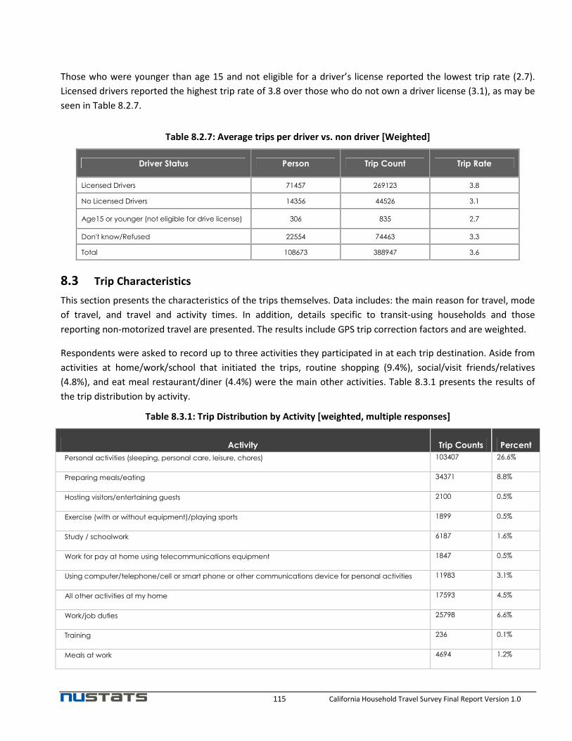
115 California Household Travel Survey Final Report Version 1.0
Those who were younger than age 15 and not eligible for a driver’s license reported the lowest trip rate (2.7).
Licensed drivers reported the highest trip rate of 3.8 over those who do not own a driver license (3.1), as may be
seen in Table 8.2.7.
Table 8.2.7: Average trips per driver vs. non driver [Weighted]
Driver Status Person Trip Count Trip Rate
Licensed Drivers 71457 269123 3.8
No Licensed Drivers 14356 44526 3.1
Age15 or younger (not eligible for drive license) 306 835 2.7
Don't know/Refused 22554 74463 3.3
Total 108673 388947 3.6
8.3 Trip Characteristics
This section presents the characteristics of the trips themselves. Data includes: the main reason for travel, mode
of travel, and travel and activity times. In addition, details specific to transit-using households and those
reporting non-motorized travel are presented. The results include GPS trip correction factors and are weighted.
Respondents were asked to record up to three activities they participated in at each trip destination. Aside from
activities at home/work/school that initiated the trips, routine shopping (9.4%), social/visit friends/relatives
(4.8%), and eat meal restaurant/diner (4.4%) were the main other activities. Table 8.3.1 presents the results of
the trip distribution by activity.
Table 8.3.1: Trip Distribution by Activity [weighted, multiple responses]
Activity Trip Counts Percent
Personal activities (sleeping, personal care, leisure, chores) 103407 26.6%
Preparing meals/eating 34371 8.8%
Hosting visitors/entertaining guests 2100 0.5%
Exercise (with or without equipment)/playing sports 1899 0.5%
Study / schoolwork 6187 1.6%
Work for pay at home using telecommunications equipment 1847 0.5%
Using computer/telephone/cell or smart phone or other communications device for personal activities 11983 3.1%
All other activities at my home 17593 4.5%
Work/job duties 25798 6.6%
Training 236 0.1%
Meals at work 4694 1.2%
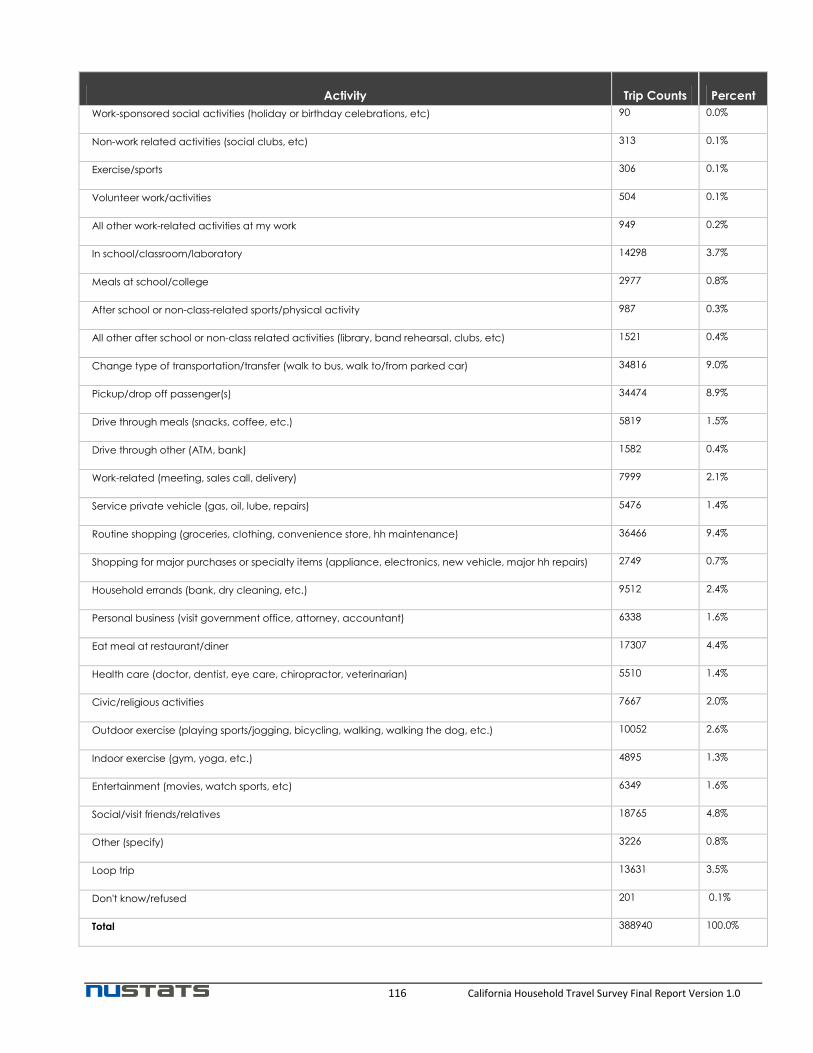
116 California Household Travel Survey Final Report Version 1.0
Activity Trip Counts Percent
Work-sponsored social activities (holiday or birthday celebrations, etc) 90 0.0%
Non-work related activities (social clubs, etc) 313 0.1%
Exercise/sports 306 0.1%
Volunteer work/activities 504 0.1%
All other work-related activities at my work 949 0.2%
In school/classroom/laboratory 14298 3.7%
Meals at school/college 2977 0.8%
After school or non-class-related sports/physical activity 987 0.3%
All other after school or non-class related activities (library, band rehearsal, clubs, etc) 1521 0.4%
Change type of transportation/transfer (walk to bus, walk to/from parked car) 34816 9.0%
Pickup/drop off passenger(s) 34474 8.9%
Drive through meals (snacks, coffee, etc.) 5819 1.5%
Drive through other (ATM, bank) 1582 0.4%
Work-related (meeting, sales call, delivery) 7999 2.1%
Service private vehicle (gas, oil, lube, repairs) 5476 1.4%
Routine shopping (groceries, clothing, convenience store, hh maintenance) 36466 9.4%
Shopping for major purchases or specialty items (appliance, electronics, new vehicle, major hh repairs) 2749 0.7%
Household errands (bank, dry cleaning, etc.) 9512 2.4%
Personal business (visit government office, attorney, accountant) 6338 1.6%
Eat meal at restaurant/diner 17307 4.4%
Health care (doctor, dentist, eye care, chiropractor, veterinarian) 5510 1.4%
Civic/religious activities 7667 2.0%
Outdoor exercise (playing sports/jogging, bicycling, walking, walking the dog, etc.) 10052 2.6%
Indoor exercise (gym, yoga, etc.) 4895 1.3%
Entertainment (movies, watch sports, etc) 6349 1.6%
Social/visit friends/relatives 18765 4.8%
Other (specify) 3226 0.8%
Loop trip 13631 3.5%
Don't know/refused 201 0.1%
Total 388940 100.0%

117 California Household Travel Survey Final Report Version 1.0
8.3.1 Mode Choice
Respondents were asked to record the mode of travel they used to make each trip. The distribution of trips by
mode collected from the survey is shown in Table 8.3.1.1. As indicated, auto was the dominant mode throughout
the region, accounting for about 76% of all trips (49.6% as drivers and 26.4% as passengers). Approximately 18%
of trips were made by non-motorized modes, and about 3% of reported trips were made by public transit.
Around 0.6% of trips were made by school bus. The distribution by travel mode is detailed in Table 8.3.1.1.
Table 8.3.1.1: Trip Distribution by Travel Mode
Mode frequency Percent
Walk 62,879 16.2%
Bike 5,943 1.5%
WheelChair/Mobility Scooter 372 0.1%
Other Non-Motorized 550 0.1%
Auto/Van/Truck Driver 192,818 49.6%
Auto/Van/Truck Passenger 102,598 26.4%
Carpool/Vanpool 2,199 0.6%
Motorcycle/Scooter/Moped 873 0.2%
Taxi/Hired Car/Limo 421 0.1%
Rental Car/Vehicle 607 0.2%
Private Shuttle 604 0.2%
Greyhound Bus 7 < 0.1%
Plane 382 0.1%
Other Private Transit 326 < 0.1%
Local Bus, Rapid Bus 10,581 2.7%
Express Bus/Commuter Bus 339 < 0.1%
Premium Bus 225 < 0.1%
School Bus 2,400 0.6%
Public Transit Shuttle 279 < 0.1%
AirBART/LAX FlyAway 12 < 0.1%
Dial-a-Ride/Paratransit 258 < 0.1%
Amtrack Bus 20 < 0.1%
Other Bus 123 < 0.1%
BART, Metro Red/Purple Line 1,834 0.5%
ACE, Amtrack, Caltrain, Coaster, Metrolink 468 0.1%
Metro Blue / Green / Gold Line, Muni Metro, Sacramento
Light Rail, San Diego Sprinter / Trolley /
Orange/Blue/Green, VTA Light Rail 1,511 0.4%
Street Car/Cable Car 100 < 0.1%
Other Rail 160 < 0.1%
Ferry/Boat 56 < 0.1%
Total 388,947 100.0%

118 California Household Travel Survey Final Report Version 1.0
Trip duration varied by mode. Overall, walk trips were the shortest, taking 10.9 minutes on average, while plane
trips took the longest at 229.9 minutes. Figure 8.3.1.1 is based on the linked trips, which included access and
egress travel by other modes for most transit modes.
Figure 8.3.1.1: Average Travel Duration by Mode
64.5
19.3
19.8
18.6
65.4
23.7
23.2
155.2
37.6
40.6
16.0
30.3
24.7
36.3
19.4
36.9
229.9
122.8
30.2
33.9
26.3
22.4
27.8
18.6
18.2
16.7
13.3
18.2
10.9
0 50 100 150 200 250
Ferry/Boat
Other Rail
Street Car/Cable Car
Metro Blue / Green / Gold Line, Muni…
ACE, Amtrack, Caltrain, Coaster,…
BART, Metro Red/Purple Line
Other Bus
Amtrack Bus
Diar-a-Ride/Paratransit
AirBART/LAX FlyAway
Public Transit Shuttle
Shool Bus
Premium Bus
Express Bus/Commuter Bus
Local Bus, Rapid Bus
Other Private Transit
Plane
Greyhound Bus
Private Shuttle
Rental Car/Vehicle
Taxi/Hired Car/Limo
Motorcycle/Scooter/Moped
Carpool/Vanpool
Auto/Van/Truck Passenger
Auto/Van/Truck Driver
Other Non-Motorized
WheelChair/MobilityScooter
Bike
Walk
Average Travel Duration (mins)

119 California Household Travel Survey Final Report Version 1.0
Looking at travel distance by travel mode in Figure 8.3.1.2, walking trips were the shortest with the average trip
length of 0.3 miles. The longest trips were made by plane – 1432.9 miles on average, which was not shown
because the extremely great value would shadow all other modes in the graph.
Figure 8.3.1.2: Average Travel Distance by Mode
19.7
5.3
3.3
5.0
33.3
9.9
5.0
83.9
6.1
19.3
2.3
4.4
6.9
12.5
3.1
15.1
79.3
9.6
17.2
6.8
7.5
10.4
6.0
5.6
0.7
0.4
1.5
0.3
0 10 20 30 40 50 60 70 80 90
Ferry/Boat
Other Rail
Street Car/Cable Car
Metro Blue / Green / Gold Line, Muni…
ACE, Amtrack, Caltrain, Coaster, Metrolink
BART, Metro Red/Purple Line
Other Bus
Amtrack Bus
Diar-a-Ride/Paratransit
AirBART/LAX FlyAway
Public Transit Shuttle
Shool Bus
Premium Bus
Express Bus/Commuter Bus
Local Bus, Rapid Bus
Other Private Transit
Greyhound Bus
Private Shuttle
Rental Car/Vehicle
Taxi/Hired Car/Limo
Motorcycle/Scooter/Moped
Carpool/Vanpool
Auto/Van/Truck Passenger
Auto/Van/Truck Driver
Other Non-Motorized
WheelChair/MobilityScooter
Bike
Walk
Average Travel Distance (miles)

120 California Household Travel Survey Final Report Version 1.0
8.3.2 Travel Times
Departure times can be grouped into time slots, representing travel in the morning peak (6 am to 10 am), midday
(10 am to 3 pm), afternoon peak (3 pm to 8 pm), night and early morning (8 pm to 6 am). Figure 8.3.2.1 is a
distribution of trips based on these travel time categories. Approximately one third of all travel (33.5%) occurred
between the mid–day hours of 10 a.m. to 2:59 p.m., while 34.3% of all travel occurred between PM peak hours
of 3 pm to 7:59 pm.
Figure 8.3.2.1: Trip Distribution by Time of Day Based on Departure Hours
In examining hourly trip distribution, the highest peak times of travel were 7 am to 8 am (8.3%) and 3 pm to 4 pm
(8.5%). These results are shown in Figure 8.3.2.2 utilizing a 24 hour time of day.
Figure 8.3.2.2: Hourly Trip Distribution by Departure Hours
23.4%
33.5% 34.3%
8.8%
0
0.05
0.1
0.15
0.2
0.25
0.3
0.35
0.4
AM Peak Midday PM Peak Night/EarlyMorning
0.1
%
0.1
%
0.1
%
0.3
%
0.9
%
2.7
%
8.3
%
7.1
%
5.3
%
5.6
%
6.3
%
6.8
%
6.6
%
8.2
%
8.5
%
7.5
%
7.8
%
6.3
%
4.3
%
3.0
% 2.1
% 1.2
% 0.6
%
0.3
%
0%
1%
2%
3%
4%
5%
6%
7%
8%
9%
10%
1 2 3 4 5 6 7 8 9 10 11 12 13 14 15 16 17 18 19 20 21 22 23 24
Time of Day (Hour)

121 California Household Travel Survey Final Report Version 1.0
8.4 Activity-Based Survey Results
For each place visited, up-to-three activities were collected. On average, two activities were reported for each
place. In detail, the average number of activities reported for the place type of Home was 1.9, the highest
overall. The results of the average number of activities by place are illustrated in Table 8.4.1.
Table 8.4.1: Average Number of Activities by Place Type (Home, Work, School and Other)
Place Type
Average Number of
Activities Counts of Trip
Places
Home 1.9 190431
Work 1.6 28817
School 1.7 19130
Other 1.1 237061
Total 1.5 475438
The average travel duration reported for the Entertainment (movies, watch sports, etc) category was 27.9
minutes, which was the longest travel duration. Respondents reported 24.4 minutes average travel duration for
the Social/visit friends/relatives category, which was the second longest travel duration. Overall, the average
travel duration was 17.8 minutes. Table 8.4.3 presents the average travel duration by activity.
Table 8.4.3: Average Travel Duration by Activity [weighted, multiple responded activities]
Activity at Visited Place Mean N
Personal activities (sleeping, personal care, leisure, chores) 18.8 108298
Preparing meals/eating 17.6 34922
Hosting visitors/entertaining guests 16.6 2119
Exercise (with or without equipment)/playing sports 17.6 1907
Study / schoolwork 15.7 6280
Work for pay at home using telecommunications equipment 15.1 1875
Using computer/telephone/cell or smart phone or other communications device for personal activities
17.0 12114
All other activities at my home 17.0 17834
Work/job duties 21.5 27880
Training 24.0 239
Meals at work 23.6 4796
Work-sponsored social activities (holiday or birthday celebrations, etc) 19.0 90
Non-work related activities (social clubs, etc) 18.7 323

122 California Household Travel Survey Final Report Version 1.0
Activity at Visited Place Mean N
Exercise/sports 22.3 309
Volunteer work/activities 16.2 507
All other work-related activities at my work 23.7 960
In school/classroom/laboratory 14.5 15514
Meals at school/college 14.0 3057
After school or non-class-related sports/physical activity 13.3 996
All other after school or non-class related activities (library, band rehearsal, clubs, etc)
16.0 1551
Change type of transportation/transfer (walk to bus, walk to/from parked
car)
17.1 34880
Pickup/drop off passenger(s) 13.9 34513
Drive through meals (snacks, coffee, etc.) 13.6 5823
Drive through other (ATM, bank) 10.8 1585
Work-related (meeting, sales call, delivery) 22.4 8135
Service private vehicle (gas, oil, lube, repairs) 17.5 5483
Routine shopping (groceries, clothing, convenience store, hh maintenance)
13.5 36556
Shopping for major purchases or specialty items (appliance, electronics,
new vehicle, major hh repairs)
17.2 2751
Household errands (bank, dry cleaning, etc.) 12.9 9537
Personal business (visit government office, attorney, accountant) 20.2 6379
Eat meal at restaurant/diner 18.8 17363
Health care (doctor, dentist, eye care, chiropractor, veterinarian) 20.7 5543
Civic/religious activities 16.3 7708
Outdoor exercise (playing sports/jogging, bicycling, walking, walking the
dog, etc.)
20.0 10135
Indoor exercise (gym, yoga, etc.) 15.2 4920
Entertainment (movies, watch sports, etc) 27.9 6394
Social/visit friends/relatives 24.4 19046
Other (specify) 25.6 3279
Loop trip 17.7 13635
Don't know/refused 14.8 202
Total 17.8 475441
The overall average number of people participated in an activity together was 1.4. The highest average amongst
the groups of people who participated in an activity together was Civic/religious category at 2.5. The average
number of people participating in an activity together was 2 or more for the following activities: After school or
non-class-related sports/physical activity; Hosting visitors/entertaining guests; Training; Work-sponsored social

123 California Household Travel Survey Final Report Version 1.0
activities (holiday or birthday celebrations, etc). Table 8.4.4 presents the average number of people who
participated in an activity together, by activity.
Table 8.4.4: Average Number of People who Participated in an Activity Together, by Activity [weighted,
multiple responded activities]
Activity at Visited Place Mean N
Personal activities (sleeping, personal care, leisure, chores) 1.2 108298
Preparing meals/eating 1.4 34922
Hosting visitors/entertaining guests 2.2 2119
Exercise (with or without equipment)/playing sports 1.2 1907
Study / schoolwork 1.1 6280
Work for pay at home using telecommunications equipment 1.1 1875
Using computer/telephone/cell or smart phone or other communications device for personal activities
1.1 12114
All other activities at my home 1.2 17834
Work/job duties 1.5 27880
Training 2.0 239
Meals at work 1.1 4796
Work-sponsored social activities (holiday or birthday celebrations, etc) 2.1 90
Non-work related activities (social clubs, etc) 1.5 323
Exercise/sports 1.4 309
Volunteer work/activities 1.7 507
All other work-related activities at my work 1.4 960
In school/classroom/laboratory 1.9 15514
Meals at school/college 1.7 3057
After school or non-class-related sports/physical activity 2.0 996
All other after school or non-class related activities (library, band rehearsal, clubs, etc) 1.9 1551
Change type of transportation/transfer (walk to bus, walk to/from parked car) 1.2 34880
Pickup/drop off passenger(s) 1.4 34513
Drive through meals (snacks, coffee, etc.) 1.3 5823
Drive through other (ATM, bank) 1.2 1585
Work-related (meeting, sales call, delivery) 1.3 8135
Service private vehicle (gas, oil, lube, repairs) 1.3 5483
Routine shopping (groceries, clothing, convenience store, hh maintenance) 1.3 36556

124 California Household Travel Survey Final Report Version 1.0
Activity at Visited Place Mean N
Shopping for major purchases or specialty items (appliance, electronics, new vehicle, major hh
repairs)
1.3 2751
Household errands (bank, dry cleaning, etc.) 1.2 9537
Personal business (visit government office, attorney, accountant) 1.2 6379
Eat meal at restaurant/diner 1.6 17363
Health care (doctor, dentist, eye care, chiropractor, veterinarian) 1.3 5543
Civic/religious activities 2.5 7708
Outdoor exercise (playing sports/jogging, bicycling, walking, walking the dog, etc.) 1.7 10135
Indoor exercise (gym, yoga, etc.) 1.5 4920
Entertainment (movies, watch sports, etc) 1.7 6394
Social/visit friends/relatives 1.7 19046
Other (specify) 1.4 3279
Loop trip 1.5 13635
Don't know/refused 1.1 202
Total 1.4 475441
8.5 Long Distance Survey Results
This section summarizes findings from the long distance trips collected from the long distance travel log only. A
total of 68,193 long distance trips were collected from 18,012 households, which is 42% of all households that
completed both recruitment and retrieval successfully. In this section, findings are based on unweighted data.
The straight-line distances between geocoded origin and destination were computed to determine approximate
travel distance. By trip purpose, combined business and pleasure trips show the longest average travel at 485.7
miles, followed by vacation/sightseeing trips (479.2 miles). Table 8.5.1 provides further details on the average
trip distance by trip purpose.
Table 8.5.1: Average Distance, and by Trip Purpose [unweighted]
Long Distance Trip Purpose
Average
Number of
Miles
Frequency of
Trips
Going to work 171.3 2815
Business (work-related meeting/convention/seminar 502.3 6193
Combined business and pleasure 485.7 1125
School -related activity 299.3 927
Visit friends/family/relatives 340.9 13067
Medical 87.8 1870
Vacation/sightseeing 479.2 7666

125 California Household Travel Survey Final Report Version 1.0
Long Distance Trip Purpose
Average
Number of
Miles
Frequency of
Trips
Outdoor recreation (sports, fishing, hunting, camping, boating, etc) 135.8 2763
Entertainment (theater, concert, sports event, gambling, etc) 141.1 2919
Personal Business (e.g. shopping) 133.3 2781
Drive someone else 105.5 1216
Return home 323.5 23223
Other (specify) 199.6 755
Don’t know 435.6 198
Refuse 183.5 85
Total 321.9 67603
The long distance log collected the travel mode used for the longest distance for each long distance trip. Looking
into travel distance by travel mode, airplane trips show the longest average travel distance at 1614.0 miles,
followed by Greyhound bus (434.8 miles). A summary of average distance by travel mode is found in Table 8.5.2.
Table 8.5.2: Average Distance and by Travel Mode (multiple responses) [unweighted]
Long distance Mode Average Number
of Miles Frequency of
Trips Walk 140.8 40
Bike 75.9 72
Wheelchair / Mobility Scooter 87.8 5
Other Non-Motorized (please specify) 228.2 4
Auto / Van / Truck Driver 125.8 47031
Auto / Van / Truck Passenger 137.5 7363
Carpool / Vanpool 137.9 499
Motorcycle / Scooter / Moped 137.3 291
Taxi / Hired Car / Limo 416.1 166
Rental Car/Vehicle 248.0 967
Private shuttle (SuperShuttle, employer, hotel, etc.) 162.6 171
Greyhound Bus 434.8 157
Plane 1614.0 8502
Other Private Transit (please specify) 285.7 234
Local Bus, Rapid Bus 73.4 88
Express Bus / Commuter Bus (AC Transbay, Golden Gate Transit, etc) 57.2 113
Premium Bus ( Metro Orange / Silver Line ) 72.1 24
School Bus 96.9 98
Public Transit Shuttle (DASH, Emery Go Round, etc.) 70.0 13
AirBART / LAX FlyAway 17.5 7

126 California Household Travel Survey Final Report Version 1.0
Long distance Mode Average Number
of Miles Frequency of
Trips Dial-a-Ride / Paratransit (Access Services, etc.) 41.2 15
Amtrak Bus 199.9 82
Other Bus (write code and specify) 210.1 105
BART, Metro Red / Purple Line 205.9 104
ACE, Amtrak, Caltrain, Coaster, Metrolink 203.4 715
Metro Blue / Green / Gold Line, Muni Metro, Sacramento Light Rail, San Diego Sprinter /
Trolley / Orange/Blue/Green, VTA 53.5 31
Street Car / Cable Car 0
Other Rail (please specify) 343.8 50
Ferry / Boat 616.1 118
DK/RF 255.6 67
Total 321.5 67132
*50 miles or longer long distance trips reported to be made by AirBART/LAX FlyAway were reclassified to the trips made by airline after
reviewing origin and destination location. AirBart.Lax FlyAway is more likely to be used as an access or an egress mode to/from an airport.
On average, approximately three persons traveled together on long distance trips. Long distance trips made by
auto/van/truck passenger travel mode averaged 3 persons. Long distance trips by airplane averaged 2 persons.
Table 8.5.3 presents the average number of travelers by travel mode.
Table 8.5.3: Average Number of Travelers by Travel Mode (multiple responses) [unweighted]
Average Number
of Travelers
Frequency of
Trips
Walk 2.0 41
Bike 2.6 68
Wheelchair / Mobility Scooter 2.6 5
Other Non-Motorized 2.0 5
Auto / Van / Truck Driver 2.1 47155
Auto / Van / Truck Passenger 2.9 7415
Carpool / Vanpool 4.2 499
Motorcycle / Scooter / Moped 1.9 286
Taxi / Hired Car / Limo 2.9 162
Rental Car/Vehicle 2.6 965
Private shuttle (SuperShuttle, employer, hotel, etc.) 6.4 169
Greyhound Bus 3.5 155
Plane 1.9 8415
Other Private Transit (please specify) 8.9 227
Local Bus, Rapid Bus 2.2 93
Express Bus / Commuter Bus (AC Transbay, Golden Gate Transit,
etc)
2.1 105
Premium Bus ( Metro Orange / Silver Line ) 6.8 23
School Bus 15.6 101
Public Transit Shuttle (DASH, Emery Go Round, etc.) 1.1 13

127 California Household Travel Survey Final Report Version 1.0
Average Number
of Travelers
Frequency of
Trips
AirBART / LAX FlyAway 3.7 31
Dial-a-Ride / Paratransit (Access Services, etc.) 5.3 15
Amtrak Bus 1.6 81
Other Bus 8.3 98
BART, Metro Red / Purple Line 2.0 103
ACE, Amtrak, Caltrain, Coaster, Metrolink 1.7 708
Metro Blue / Green / Gold Line, Muni Metro, Sacramento Light
Rail, San Diego Sprinter / Trolley / Orange/Blue/Green, VTA
1.9 31
Street Car / Cable Car 0
Other Rail 3.1 50
Ferry / Boat 2.6 113
DK/RF 2.2 50.0
Total 2.3 67175
Excluding “returning home” trips, 96.9% of trip destinations were within the United States. Mexico is ranked as
the second most popular long distance trip destination with a 0.7% share, followed by Canada with 0.4% of trips
having ended in Canada. The top 10 destinations by country are ranked in Table 8.5.4.
Table 8.5.4: Top 10 Destination Countries [unweighted]
Destination Countries Percent
United states 96.9%
Mexico 0.7%
Canada 0.4%
United kingdom 0.2%
Italy 0.1%
France 0.1%
Germany 0.1%
Japan 0.1%
China 0.1%
India 0.1%
Other counties 1.1%
Total 100.0%
Excluding “returning home” trips, 79.2% of trip destinations were within the state of California. Looking at
destination cities in detail, 4.6% of trips were destined for San Francisco, followed by Los Angeles (4.2%) and
Sacramento (2.9%). Table 8.5.5 gives a summary of the results for the top 50 destination cities.

128 California Household Travel Survey Final Report Version 1.0
Table 8.5.5: Top 50 Destination Cities [unweighted]
Destination Cities Percent
San Francisco 4.6%
Los Angeles 4.2%
Sacramento 2.9%
San Diego 2.7%
San Jose 1.9%
Las Vegas 1.7%
Reno 1.4%
Fresno 1.3%
Oakland 1.1%
Anaheim 0.9%
Bakersfield 0.9%
Santa Rosa 0.8%
Santa Barbara 0.8%
Redding 0.7%
Santa Cruz 0.7%
Stockton 0.7%
Monterey 0.6%
Long Beach 0.6%
Modesto 0.5%
Palm Springs 0.5%
Berkeley 0.5%
South Lake Tahoe 0.5%
San Luis Obispo 0.5%
Napa 0.5%
Davis 0.5%
Destination Cities Percent
Irvine 0.4%
Chico 0.4%
Ventura 0.4%
New York 0.4%
Santa Clara 0.4%
Santa Ana 0.4%
Truckee 0.4%
Carlsbad 0.4%
Palo Alto 0.4%
Seattle 0.4%
Yosemite National Park 0.4%
Portland 0.4%
Riverside 0.3%
Pasadena 0.3%
Palm Desert 0.3%
Roseville 0.3%
Temecula 0.3%
Lancaster 0.3%
Phoenix 0.3%
Salinas 0.3%
Santa Maria 0.3%
Newport Beach 0.3%
Santa Monica 0.3%
Ontario 0.3%
Santa Clarita 0.3%
For those who reported traveling via airplane, rail or bus for their long distance trip, access mode to the
departure airport or station was asked. The most popular mode of access for departing trips (all trips excluding
returning home trips) was auto driver (34.5%) or passenger (27.7%). Taxis followed with 6.3% of the share.
Access mode to the departure airport or station is presented in Table 8.5.6.

129 California Household Travel Survey Final Report Version 1.0
Table 8.5.6: Access Mode to the Departure Airport/Station (Base=Outbound Trips Made by bus/rail/airplane)
Departure Mode Count
Column
N %
Walk 49.0 3.9%
Bike 2.0 .2%
Auto / Van / Truck Driver 436.0 34.5%
Auto / Van / Truck Passenger 350.0 27.7%
Carpool / Vanpool 3.0 .2%
Taxi / Hired Car / Limo 80.0 6.3%
Rental Car/Vehicle 16.0 1.3%
Private shuttle (SuperShuttle, employer, hotel, etc.) 23.0 1.8%
Greyhound Bus 5.0 .4%
Plane 19.0 1.5%
Other Private Transit 5.0 .4%
Local Bus, Rapid Bus 26.0 2.1%
Express Bus / Commuter Bus (AC Transbay, Golden Gate Transit, etc) 5.0 .4%
Premium Bus ( Metro Orange / Silver Line ) 3.0 .2%
Public Transit Shuttle (DASH, Emery Go Round, etc.) 5.0 .4%
AirBART / LAX FlyAway 7.0 .6%
Amtrak Bus 3.0 .2%
Other Bus (write code and specify) 6.0 .5%
BART, Metro Red / Purple Line 15.0 1.2%
ACE, Amtrak, Caltrain, Coaster, Metrolink 5.0 .4%
Metro Blue / Green / Gold Line, Muni Metro, Sacramento Light Rail, San Diego Sprinter / Trolley /
Orange/Blue/Green, VTA
2.0 .2%
Other Rail 3.0 .2%
Don’t Know/Refused 196.0 15.5%
For trips made by airplane, bus or rail for the return home, auto driver (21.5%) or passenger (17.2%) were again
the most likely means of transportation used to access the departure airport or bus/rail station. Taxis followed
with 4.5% of the share. Table 8.5.7 details the egress mode to the arrival airport or station.
Table 8.5.7: Egress Mode to the Arrival Airport/Station (Base=Returning Home Trips Made by bus/rail/airplane)
Arrival Mode Count Column N %
Walk 7 1.2%
Wheelchair / Mobility Scooter 1 .2%
Other Non-Motorized (please specify) 1 0.2%
Auto / Van / Truck Driver 130 21.5%
Auto / Van / Truck Passenger 104 17.2%
Carpool / Vanpool 2 0.3%

130 California Household Travel Survey Final Report Version 1.0
Arrival Mode Count Column N %
Taxi / Hired Car / Limo 27 4.5%
Rental Car/Vehicle 10 1.7%
Private shuttle (SuperShuttle, employer, hotel, etc.) 9 1.5%
Plane 14 2.3%
Other Private Transit (please specify) 2 .3%
Local Bus, Rapid Bus 2 0.3%
Express Bus / Commuter Bus (AC Transbay, Golden Gate Transit, etc) 1 .2%
Public Transit Shuttle (DASH, Emery Go Round, etc.) 1 .2%
AirBART / LAX FlyAway 4 .7%
Other Bus (write code and specify) 2 .3%
BART, Metro Red / Purple Line 10 1.7%
ACE, Amtrak, Caltrain, Coaster, Metrolink 3 .5%
Metro Blue / Green / Gold Line, Muni Metro, Sacramento Light Rail, San
Diego Sprinter / Trolley / Orange/Blue/Green, VTA
1 0.2%
Other Rail (please specify) 2 .3%
DK/RF 274 45.3%
Total 605 100.0%
When looking at the days of the week reported for long distance trips, the majority of participants reported they
traveled on Saturday (18.8%) and Sunday (17.3%). Tuesday and Wednesday were reported as the least popular
days for long distance travel with 11.1% and 11.7%, respectively. Figure 8.5.1 presents the distribution of long
distance trips by day of week.
Figure 8.5.1: Distribution of Long Distance Trips by Day of the Week
12.3%11.1%
11.7%12.6%
16.3%
18.8%
17.3%
0%
5%
10%
15%
20%
Monday Tuesday Wednesday Thursday Friday Saturday Sunday
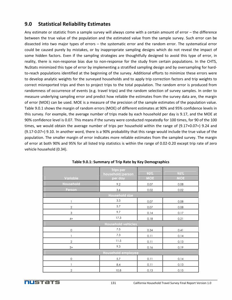
131 California Household Travel Survey Final Report Version 1.0
9.0 Statistical Reliability Estimates
Any estimate or statistic from a sample survey will always come with a certain amount of error – the difference
between the true value of the population and the estimated value from the sample survey. Such error can be
dissected into two major types of errors – the systematic error and the random error. The systematical error
could be caused purely by mistakes, or by inappropriate sampling designs which do not reveal the impact of
some hidden factors. Even if the sampling strategies are thoughtfully designed to avoid this type of error, in
reality, there is non-response bias due to non-response for the study from certain populations. In the CHTS,
NuStats minimized this type of error by implementing a stratified sampling design and by oversampling for hard-
to-reach populations identified at the beginning of the survey. Additional efforts to minimize these errors were
to develop analytic weights for the surveyed households and to apply trip correction factors and trip weights to
correct misreported trips and then to project trips to the total population. The random error is produced from
randomness of occurrence of events (e.g. travel trips) and the random selection of survey samples. In order to
measure underlying sampling error and predict how reliable the estimates from the survey data are, the margin
of error (MOE) can be used. MOE is a measure of the precision of the sample estimates of the population value.
Table 9.0.1 shows the margin of random errors (MOE) of different estimates at 90% and 95% confidence levels in
this survey. For example, the average number of trips made by each household per day is 9.17, and the MOE at
90% confidence level is 0.07. This means if the survey were conducted repeatedly for 100 times, for 90 of the 100
times, we would obtain the average number of trips per household within the range of (9.17+0.07=) 9.24 and
(9.17-0.07=) 9.10. In another word, there is a 90% probability that this range would include the true value of the
population. The smaller margin of error indicates more reliable estimates from the sampled survey. The margin
of error at both 90% and 95% for all listed trip statistics is within the range of 0.02-0.20 except trip rate of zero
vehicle household (0.34).
Table 9.0.1: Summary of Trip Rate by Key Demographics
Variable
Trips per
household/person
per day
90% 95%
MOE MOE
Household 9.2 0.07 0.08
Person 3.6 0.02 0.02
Household size
1 3.3 0.07 0.08
2 5.7 0.07 0.08
3 9.7 0.14 0.17
4+ 17.3 0.18 0.21
Household vehicles
0 7.5 0.34 0.41
1 7.3 0.11 0.14
2 11.5 0.11 0.13
3+ 9.3 0.16 0.19
Household employee
0 5.7 0.11 0.14
1 8.4 0.11 0.13
2 10.8 0.13 0.15

132 California Household Travel Survey Final Report Version 1.0
Variable
Trips per
household/person
per day
90% 95%
MOE MOE
3+ 18.4 0.3 0.36
Income Level
Less than $24,999 8.6 0.20 0.24
$25,000 - $49,999 8.6 0.16 0.19
$50,000 - $74,999 9.0 0.16 0.20
$75,000 - $99,999 10.5 0.18 0.22
$100,000 - $149,999 11.0 0.18 0.21
$150,000 or above 8.6 0.20 0.24
Gender
Male 3.4 0.02 0.03
Female 3.7 0.02 0.03
Age
Less than 20 years 3.3 0.03 0.03
20 - 34 years 3.5 0.05 0.06
35 - 54 years 4.3 0.04 0.04
55 - 64 years 3.7 0.04 0.05
65 years or older 2.9 0.04 0.05
Hispanic or Latino
Yes 3.5 0.03 0.04
No 3.6 0.02 0.02
Race
White 3.6 0.02 0.02
Black or African American 3.5 0.11 0.13
American Indian or Alaska Native 3.7 0.08 0.09
Asian 3.5 0.07 0.08
Native Hawaiian or Pacific Islander 3.4 0.3 0.36
Employment
Yes 4.0 0.02 0.03
No 3.2 0.03 0.04
Driver License
Yes 3.8 0.02 0.02
No 3.1 0.08 0.09

133 California Household Travel Survey Final Report Version 1.0
10.0 Limitations of the Survey
As with any survey dataset, there are limitations on its use. End users must understand the methods used to
collect the data, the accuracy when analyzing at the subsample level, and various biases. Each of these affects
the reliability level when generalizing to their desired population. These limitations are described below.
Under-Representation of Cell Phone Only Households
Surveys are prone to non–response errors because certain types of households selected in a sample do not
participate in surveys. The main sampling frame for the CHTS was address-based, which yielded household
addresses for which either a telephone number was attached (matched) or address for which there was no
telephone number associated (unmatched). These latter households are predominately cell-phone-only
households. A 2011 study by the National Center for Health Statistics5 showed that the percentage of wireless
only households was significantly increasing among younger, poorer and more mobile households; they
estimated 18% of California households were cell phone only.
As may be seen from Table 10.1, unmatched households were sampled at a higher rate (28%), but they were a
far lower percentage of recruited households (4.7%). Recall that unmatched households were sent an advance
letter that contained a PIN directing them to recruit online, and a telephone number for them to recruit by
telephone. This was the only contact with these households. The CHTS is not the only survey that has an under-
representation of cell phone only households; this is an issue for survey research firms nationwide. Some of the
suggested remedies include using smart phone applications as another response mode, and being more active in
the use of social media to promote the survey.
Table 10.1: Recruitment and Response Rate by Sample Type
Sample
Type
Sample Used in Main
Survey Recruited Households Retrieved Households
Number
(A)
% of
Total
Number
(B)
% of
Total
Recruitment
Rate
(B)/(A)
Number
(C)
% of
Total
Retrieval
Rate
(C')/(B)
ABS
Matched/
Listed
1,410,365 66.5% 58658 93.0% 4.2% 38934 91.8% 66.4%
Unmatched 585520 27.6% 2996 4.7% 0.5% 2458 5.8% 82.0%
Energy
Commission
Samples
121835 5.7% 985 1.6% 0.8% 809 1.9% 82.1%
Kern
County
Transit
Intercept
1353 0.1% 443 0.7% 32.7% 230 0.5% 51.9%
Total 2,119,073 100.0% 63082 100.0% 3.0% 42431 100.0% 67.3%
Language Limitations
The main survey was conducted in Spanish which, as discussed in Section 4.0, involved translating all of the
survey printed materials (diary and GPS) as well as the CATI and online scripts into Spanish. As it turned out, only
5 Accessed May 22, 2013: http://www.cdc.gov/nchs/data/nhis/earlyrelease/wireless201112.htm

134 California Household Travel Survey Final Report Version 1.0
5,543 households requested at the end of the recruitment interview to receive the Spanish version of the
recruitment package. This was less than 1% of the recruited households, and indicated that the majority of
Hispanic households that participated in the CHTS preferred the English versions.
At the same time, 1.4% of all sampled households were unable to be recruited due to the use of languages other
than English or Spanish. In California, there are many areas with linguistically isolated households speaking a
variety of languages such as Chinese, Tagalog, Vietnamese, Korean, Persian, Armenian and many more. While the
percentage speaking any one of these languages was much lower than 1.4% on a statewide basis, there may
have been local areas in which the percentage of a language was much higher.
From a statewide survey resource allocation point of view, the time and effort involved in translating materials
into a language that was likely to be used by a small fraction of households was greater than the benefit in
additional households. However, it must be acknowledged that there may have been certain geographies in the
state in which the lack of materials in a key language may have served as a limitation to participation.
Limitation in Long Distance Data
To increase the use of the long distance log, with the concurrence of Caltrans and the Expert Pretest Review
Panel, the long distance logs were extensively reformatted after the pretest, as was discussed in Section 4.0.
Specifically, the questions asking for how participants travelled to the departure/arrival airport or station (mode
of access and egress) for long distance trips made by transit, and the name of the airport, bus or train station,
were removed from the printed log for the main survey. These questions continued to be asked for the most
recent long distance trip only in the CATI and online scripts.
In August, 2012 the concern was raised that the removal of the access and egress information from being
collected on every long distance trip involving transit use would severely limit the use of the data for certain
travel demand models. The consensus was it was too late to make the changes to the scripts and printed
materials necessary to collect the access and egress information on all long distance trips at that point in the
main survey data collection. The absence of the access and egress data is noted by a DK in the dataset and, for
those modelers seeking this information, remains a limitation.
Caution in Using Weights and Trip Correction Factor
The final weights were developed at the county level, but demographic controls were balanced at the statewide
level only. Also trip correction factors for the CHTS were developed at the statewide level only. Users of the CHTS
final data are cautioned in applying these weights to lower level geographies, such as sampling strata, counties or
MPO.
Process for Performing OBD Weighting
Sampling weights for the CHTS were computed to address sampling bias and non-response bias. More detail with
regard to the weighting procedure may be found in Section 7.0. Sampling weights were computed based on the
randomly drawn sample. Taking the base weights of these sampling weights, the sampling weights were then
balanced with the control totals of key demographic variables from either the general population Energy
Commission OBD GPS samples (drawn from the Energy Commission database of alternative fuel vehicle owners)
or the UC Davis database of alternative fuel vehicle owners. The sample pulled from these databases was not
pulled in a random draw. Additionally, overlap between these two databases and the ABS sampling frame or
listed sampling frame is unknown. Also, this sample was not drawn randomly by geography. Therefore, there was
no adjustment made at the sample unit level for Energy Commission GPS sample. However, Energy Commission
GPS samples were included in the raking procedure to control representation of survey sample to the general
population. All survey complete samples, including Energy Commission GPS sample, were controlled under key
demographic variables from the latest general population data.

135 California Household Travel Survey Final Report Version 1.0
11.0 Recommendations for Future Survey Improvement
In a large, complex, and lengthy effort such as the CHTS, there were a number of lessons learned and
recommendations for future survey improvement. This section presents the collective lessons learned and
recommendations for the next California statewide travel survey.
Survey Administration and Governance: To conduct the CHTS, transportation planning and environmental
agencies around the state came together to pool their resources to develop a common survey that could be used
for many purposes. Having a single, common survey meant that a single contractor would be responsible for data
collection, which ensured that the survey methods were consistent, as were the resulting data and data
elements. A single, statewide effort also allowed participating agencies to share and build staff experience and
expertise and share the costs of survey development, which is one of the more costly aspects of conducting a
survey.
From a governance and process point of view, there were many aspects that worked well, such as:
• The committee structure developed to support the CHTS --having an Administrative Committee as well
as the larger Steering Committee ensured decisions were discussed and made by the appropriate and
informed group.
• The use of expert advisors to provide technical guidance in the development of the survey design as part
of the request for proposal, and throughout the survey process;
• The use of a facilitator for the Administrative and Steering Committee meetings -- helped to streamline
meetings, and to ensure there was opportunity for everyone to have a voice in the project.
There were some aspects of the CHTS survey administration that did not work as well as they could have, and
recommendations for future studies include:
Recommendation 1: Ensure that the contracting process allows for flexibility and change, especially in large,
complex surveys or surveys that span a long period.
Recommendation 2. Extend the survey timeline to: a) add more time for coordination and decision making when
there are many partner agencies, and b) add more time between the pretest and the main survey to permit
thorough review and changes to be made and re-tested, if needed.
Public Outreach: The need for public outreach and awareness of the survey effort cannot be overemphasized.
Travel behavior surveys ask questions that are considered intrusive by many potential respondents, and having a
level of awareness that the survey is a legitimate effort can only assist in increasing the response rate. This is
especially true for groups that are typically under-represented, including travelers that are young, Hispanic,
and/or low-income.
Recommendation 3: Incorporate a comprehensive outreach program into the survey design and process early on,
whether the outreach is to be conducted by the sponsoring agency(cies) or by the survey contractor.
The outreach effort, whether executed by sponsoring agency staff or by the contractor, should be part of the
survey design planning. If agency public relations staff are to execute the outreach, these staff should be part of
the survey design team and play an active role in the survey from the beginning of the design discussions
through to the end of data collection. If the public outreach effort execution is going to be the responsibility of
the survey contractor, this should be spelled out in the RFP, an appropriate level of the survey budget should be
applied to this effort, and the outreach effort and execution activities and timeline should be part of the survey
contract.

136 California Household Travel Survey Final Report Version 1.0
Data Collection Techniques: Household travel surveys appear to be at a significant crossroads in terms of
collecting primary data through surveys and increasing the use of secondary data "big data." There are likely to
be many changes to the need for different types of information, and the methods to collect it.
Recommendation 4: Incorporate new data collection practices and methods, such as smart phones, enhanced and
customized online surveys, expanded OBD devices, as well as the use of secondary data such as cell phone traces,
to increase survey response modes and reduce respondent burden.
Recommendation 5: Recognize the need to continue to provide incentives, regardless of continued concern over
the use of "tax payer" monies, but incorporate newer options such as digital currency or customized electronic gift
cards.
Recommendation 6: Work to keep the respondent burden to a reasonable level even if it means collecting some
data elements, such as the long distance trips, in a separate, follow-on survey.
The CHTS was a long and complex survey both to administer and for the respondents. There can be no question
that the response rate and the number of completed households would have been higher with fewer questions.
Periodic or Continuous Surveys: It is a major undertaking for multiple agencies to pool their resources and come
to consensus on a larger statewide travel survey. Planning for the CHTS started in 2008, two years before the RFP
was issued, and the survey funding remained in motion even after data collection began. Rather than expending
staff resources and saving up monetary resources for a once in a decade effort, it would smooth out the effort
and require less funding at any given time if the California statewide travel survey was on a continuous or more
frequent cycle. The cost per year is lower, and there is the distinct advantage that staff will have time to build up
their survey skills. An alternative to a continuous survey is to conduct smaller surveys on a periodic schedule,
perhaps every two to three years.
Recommendation 7: Consider conducting the California statewide travel survey on a continuous or more frequent
cycle, rather than once every ten years.
Public Use Data: Over the past several years, there has been increased scrutiny of households travel behavior
surveys in terms of the use of personally identifiable information and privacy issues. Most frequently at issue is
access to the detailed personally identifiable information (PII) that is collected about each household, person and
trip. When the CHTS was being planned, in 2008 and 2009, these issues were just coming to the forefront. But
the time this report was written in 2013, the need for security around PII was high, and there were real concerns
over how much of the collected data could be made available to research organizations other than those that
had participated in the study.
Recommendation 8: Plan the data sharing protocols for different levels of users in advance.
The desired data sharing protocols should be determined in advance of data collection, and the respondent
consent statement should reflect the desired data sharing.
GPS Subsample
In the technical proposal for this study, NuStats offered an alternate solution in addition to the method of GPS
data collection that was ultimately used in the study. This alternate solution suggested the use of GPS-only
passive data collection with no paper diary, then a prompted recall interview in order to gather the uncollected
diary data. NuStats has since found that in order for the prompted recall to be successful, the respondent still
requires some sort of memory jogger in place of the travel diary.

137 California Household Travel Survey Final Report Version 1.0
A solution to this need for memory joggers would be to put more effort into developing trip detection algorithms
such as the one used in this study, so that prompted recall is not necessary. These algorithms are becoming more
and more sophisticated and can impute not only trip origin and destination points from raw GPS data; they can
also impute trip mode and purpose. Used in conjunction with rich georeferenced road & path, land use, and
recruit information databases, trip detection tools can produce highly accurate results and do not require
significant supplementation by trip diaries.
The less preferred way of reducing the amount of prompted recall required in a GPS survey is to have an active
device which requires some sort of respondent input while traveling. Active devices have been shown to affect a
respondent’s ability to capture a complete set of data as they come with a larger burden. Current active GPS
devices call for the respondent to answer specific questions about each trip during the travel period and/or start
and stop the device when beginning and ending travel. However, there are GPS devices available that can
passively collect GPS data and also have the option to record time-and geographically-tagged voice notes. A
quick recording of the respondent saying “home”, “work”, “school”, or any other relevant information when a
stop is made can be converted from voice to text and documented at that geographic location in the data file.
These devices are comparable in price to completely passive ones and offer a hybrid approach that is minimally
burdensome on the respondent and can still provide some mode/purpose data.
Another suggestion for future studies not listed in the technical proposal, but that has since the beginning of the
Caltrans survey become an increasingly attractive option, would be to use passive smartphone GPS data
collection applications which transmit GPS location traces wirelessly to the data servers. Offering respondents
the option to use their personal smartphone in travel surveys not only reduces the amount of money spent on
device purchase and shipping, but also provides respondents with a familiar, fatigue-free medium for data
collection. In addition, smartphones’ wireless data transmission capability offers the surveyor freedom to
conduct long-term studies as device memory is not a limitation, and also decreases the amount of time that must
be invested in data uploading. There is no potential for unreturned devices with surveys done on personal
smartphones, and a respondent’s data usage is more than compensated for with the incentive. These
applications can also retrieve information from wireless and Bluetooth OBD sensors. More work must be done to
adapt applications such as these to all smartphone models and operating systems, but the flexibility and
potential provided by this technology is extremely great.