1 

Vector Addition 

Equipment ListQty  Item  Part Number 

1  Force Table   ME‐9447B 

1  Mass and Hanger Set  ME‐8979 

1  Carpenter’s level 

1  String 

PurposeThe purpose of this lab is for the student to gain a better understand of the basic properties of vectors, 

and some simple vector mathematics. The student will see how vectors are related to the Right Triangle, 

and how vectors can be described in both the Rectangular Coordinate system, and the Polar Coordinate 

system. Also, the student will see how to convert a vector from one coordinate system to the other, and 

then back again. By adding different combinations of force vectors, and adding those vectors by 

different means, the student’s understanding of vectors, and vector addition, should be improved. 

Theory The Right Triangle, and Simple Trig Functions A triangle is a three sided, closed, geometric shape, whose three internal angles sum to 180o. A Right 

Triangle is a triangle that one of its internal Angles is 90o, which is called a right angle. If we pick one of 

the other two internal angles of a right triangle, and call it θ (theta), then we are able to label the three 

sides of the right triangle in reference to the angle θ. 

The three sides are: 

1. Hypotenuse (hyp) – The side that is opposite the right angle, and it is ALWAYS the longest of the

three sides.

2. Adjacent (adj) – This along with the hypotenuse forms the angle θ.

3. Opposite (opp) – The side that is opposite of the angle θ.

Trig Functions relate the value of the angle θ to the value of the ratio of the lengths of two of the sides of 

a right triangle. There are three basic Trig Functions.  

rev 09/2019

2  

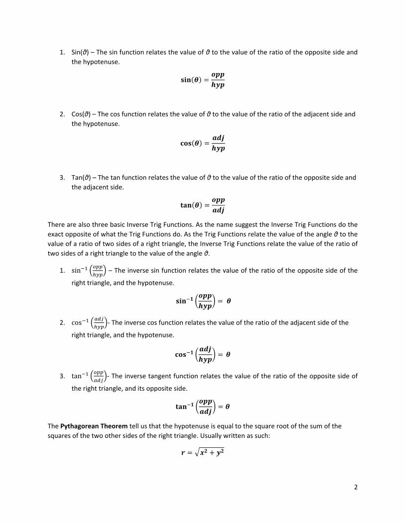
1. Sin(θ) – The sin function relates the value of θ to the value of the ratio of the opposite side and 

the hypotenuse. 

𝐬𝐢𝐧 𝜽𝒐𝒑𝒑𝒉𝒚𝒑

 

 

2. Cos(θ) – The cos function relates the value of θ to the value of the ratio of the adjacent side and 

the hypotenuse.  

𝐜𝐨𝐬 𝜽𝒂𝒅𝒋𝒉𝒚𝒑

 

 

3. Tan(θ) – The tan function relates the value of θ to the value of the ratio of the opposite side and 

the adjacent side.  

𝐭𝐚𝐧 𝜽𝒐𝒑𝒑𝒂𝒅𝒋

 

There are also three basic Inverse Trig Functions. As the name suggest the Inverse Trig Functions do the 

exact opposite of what the Trig Functions do. As the Trig Functions relate the value of the angle θ to the 

value of a ratio of two sides of a right triangle, the Inverse Trig Functions relate the value of the ratio of 

two sides of a right triangle to the value of the angle θ. 

1. sin  – The inverse sin function relates the value of the ratio of the opposite side of the 

right triangle, and the hypotenuse. 

𝐬𝐢𝐧 𝟏 𝒐𝒑𝒑𝒉𝒚𝒑

𝜽 

2. cos ‐ The inverse cos function relates the value of the ratio of the adjacent side of the 

right triangle, and the hypotenuse. 

𝐜𝐨𝐬 𝟏 𝒂𝒅𝒋𝒉𝒚𝒑

𝜽 

3. tan ‐ The inverse tangent function relates the value of the ratio of the opposite side of 

the right triangle, and its opposite side. 

𝐭𝐚𝐧 𝟏 𝒐𝒑𝒑𝒂𝒅𝒋

𝜽 

The Pythagorean Theorem tell us that the hypotenuse is equal to the square root of the sum of the 

squares of the two other sides of the right triangle. Usually written as such: 

𝒓 𝒙𝟐 𝒚𝟐 

 

3  

 

 

Coordinate Systems There are two basic coordinate systems we will be working with in this lab: the rectangular coordinate 

system, and the polar coordinate system. 

 

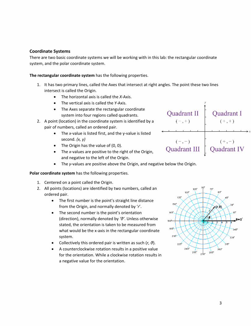
The rectangular coordinate system has the following properties. 

1. It has two primary lines, called the Axes that intersect at right angles. The point these two lines 

intersect is called the Origin. 

The horizontal axis is called the X‐Axis. 

The vertical axis is called the Y‐Axis. 

The Axes separate the rectangular coordinate 

system into four regions called quadrants. 

2. A point (location) in the coordinate system is identified by a 

pair of numbers, called an ordered pair. 

The x‐value is listed first, and the y‐value is listed 

second. (x, y) 

The Origin has the value of (0, 0). 

The x‐values are positive to the right of the Origin, 

and negative to the left of the Origin. 

The y‐values are positive above the Origin, and negative below the Origin. 

Polar coordinate system has the following properties. 

1. Centered on a point called the Origin. 

2. All points (locations) are identified by two numbers, called an 

ordered pair. 

The first number is the point’s straight line distance 

from the Origin, and normally denoted by ‘r’. 

The second number is the point’s orientation 

(direction), normally denoted by ‘θ’. Unless otherwise 

stated, the orientation is taken to be measured from 

what would be the x‐axis in the rectangular coordinate 

system. 

Collectively this ordered pair is written as such (r, θ). 

A counterclockwise rotation results in a positive value 

for the orientation. While a clockwise rotation results in 

a negative value for the orientation.  

 

 

 

4  

 

 

Converting between coordinate systems 

Sometimes we have a point that is described by one coordinate system, but for various mathematical 

reasons we need it to be described by another coordinate system. So we must convert between 

coordinate systems. We can, and will, use the properties of the Right Triangle to convert between our 

polar and rectangular coordinate systems.  

 

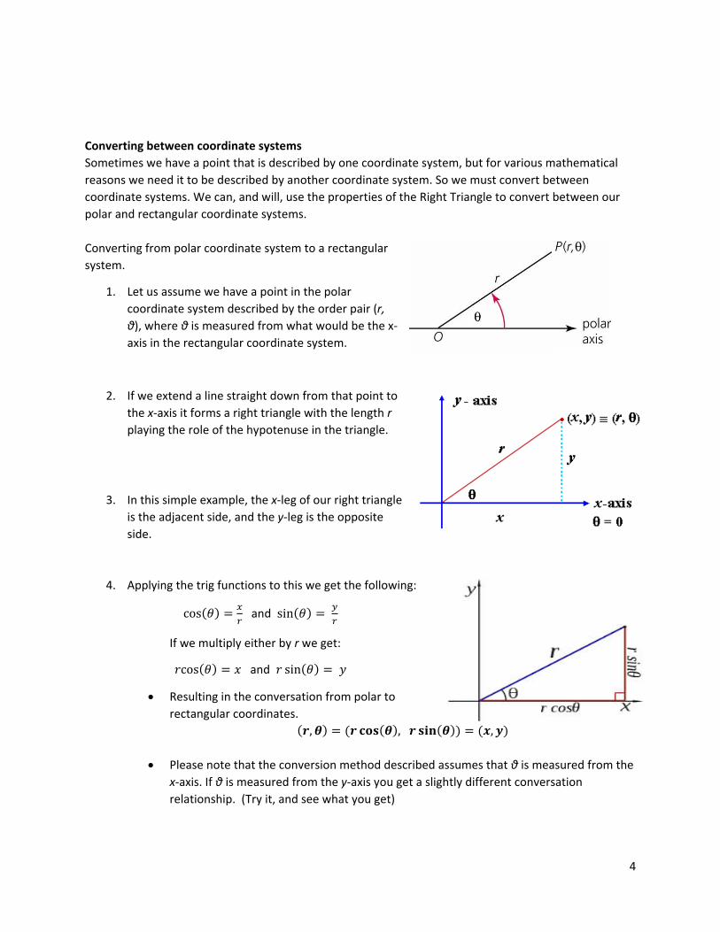
Converting from polar coordinate system to a rectangular 

system.  

1. Let us assume we have a point in the polar 

coordinate system described by the order pair (r, 

θ), where θ is measured from what would be the x‐

axis in the rectangular coordinate system. 

 

2. If we extend a line straight down from that point to 

the x‐axis it forms a right triangle with the length r 

playing the role of the hypotenuse in the triangle.  

  

 

3. In this simple example, the x‐leg of our right triangle 

is the adjacent side, and the y‐leg is the opposite 

side. 

 

 

4. Applying the trig functions to this we get the following: 

cos 𝜃    and  sin 𝜃  

    If we multiply either by r we get: 

𝑟cos 𝜃 𝑥   and  𝑟 sin 𝜃 𝑦 

Resulting in the conversation from polar to 

rectangular coordinates. 

𝒓, 𝜽 𝒓 𝐜𝐨𝐬 𝜽 , 𝒓 𝐬𝐢𝐧 𝜽 𝒙, 𝒚  

 

Please note that the conversion method described assumes that θ is measured from the 

x‐axis. If θ is measured from the y‐axis you get a slightly different conversation 

relationship.  (Try it, and see what you get) 

 

 

5  

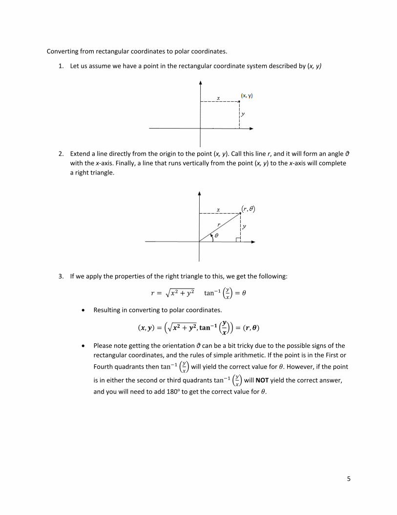
Converting from rectangular coordinates to polar coordinates.  

1. Let us assume we have a point in the rectangular coordinate system described by (x, y) 

 

 

 

 

 

2. Extend a line directly from the origin to the point (x, y). Call this line r, and it will form an angle θ 

with the x‐axis. Finally, a line that runs vertically from the point (x, y) to the x‐axis will complete 

a right triangle.  

 

 

 

 

 

 

 

 

 

 

3. If we apply the properties of the right triangle to this, we get the following: 

𝑟 𝑥 𝑦       tan 𝜃 

Resulting in converting to polar coordinates. 

𝒙, 𝒚 𝒙𝟐 𝒚𝟐, 𝐭𝐚𝐧 𝟏 𝒚𝒙

𝒓, 𝜽  

Please note getting the orientation θ can be a bit tricky due to the possible signs of the 

rectangular coordinates, and the rules of simple arithmetic. If the point is in the First or 

Fourth quadrants then tan  will yield the correct value for 𝜃. However, if the point 

is in either the second or third quadrants tan  will NOT yield the correct answer, 

and you will need to add 180o to get the correct value for 𝜃.  

 

 

 

 

 

6  

Vectors and Right Triangles A vector is a mathematical ‘object’ that has both a magnitude (size), and a direction, and it requires at 

least two numbers to describe a vector. There are two basic  forms that those two bits of  information 

about a vector are written in; Pure Form, or Component Form.  

1. The Pure Form is called that because the two pieces of information about the vector, magnitude, 

and  directions  are  completely  separated  from  each  other.  So  one  number  gives  you  purely 

information about the magnitude, and the other number gives you purely information about the 

direction.  

Let’s assume we have a vector 𝑉, then in pure form it would be written as 𝑉 𝑉, 𝜃  

Where the first number V is the magnitude, while the second number θ is the direction 

of the vector.  

 

2. The Component Form still describes the vector by using two numbers, but the information about 

magnitude, and direction are sort of ‘mixed up’ between both of the numbers.  

Let’s assume the same vector 𝑉 as before is written in component form instead, then that 

would be �⃗� 𝑉 , 𝑉 . 

The first number 𝑉  is displacement in the x‐direction, and the second number 𝑉  is the 

displacement in the y‐direction.  

 

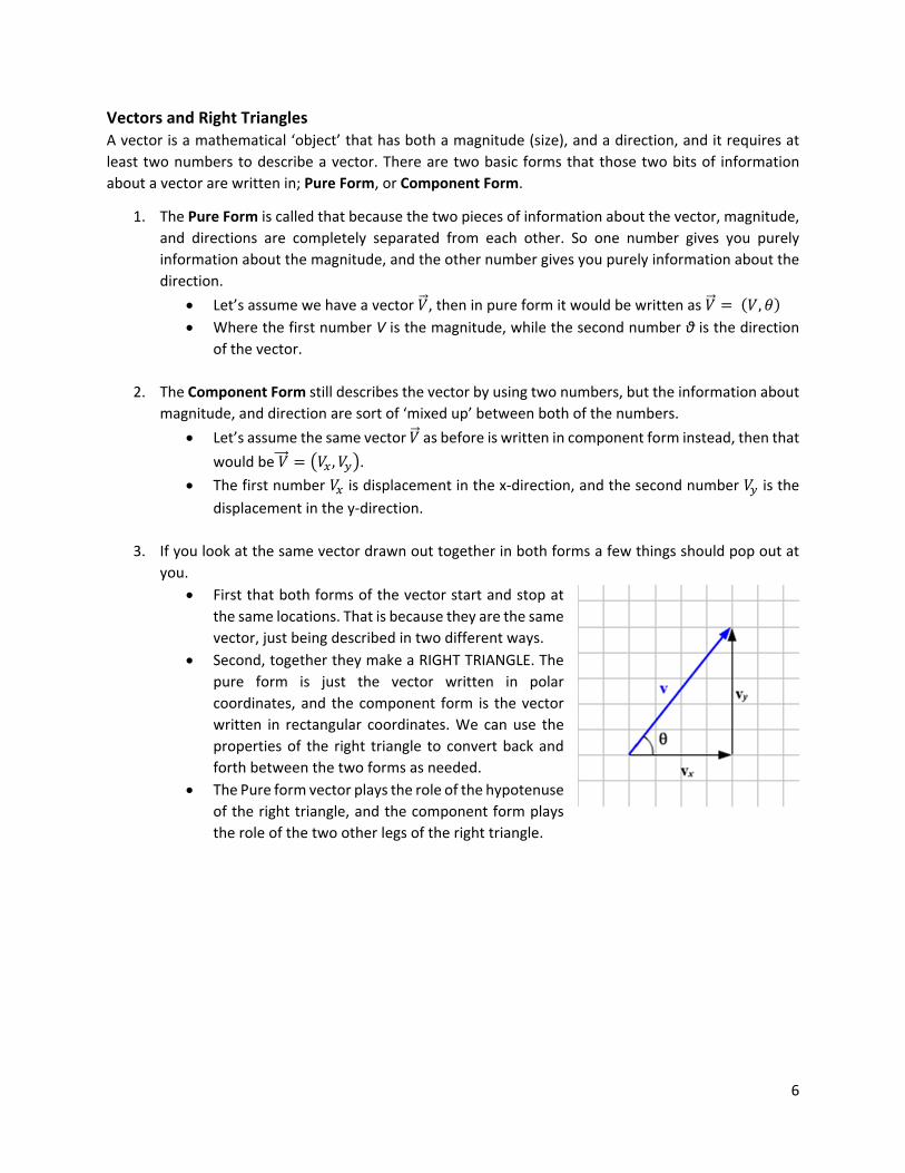
3. If you look at the same vector drawn out together in both forms a few things should pop out at 

you. 

First that both forms of the vector start and stop at 

the same locations. That is because they are the same 

vector, just being described in two different ways. 

Second, together they make a RIGHT TRIANGLE. The 

pure  form  is  just  the  vector  written  in  polar 

coordinates,  and  the component  form  is  the vector 

written  in  rectangular  coordinates. We  can use  the 

properties of  the  right  triangle  to  convert back and 

forth between the two forms as needed.  

The Pure form vector plays the role of the hypotenuse 

of the right triangle, and the component form plays 

the role of the two other legs of the right triangle. 

 

 

 

 

 

7  

Adding Vectors 

The summation of a set of vectors is called the resultant vector. We will be examining three different 

methods of adding vectors to obtain the resultant vector: graphical, mathematical and experimental. 

Regardless of the method used when adding a set of vectors, one should obtain the same resultant.  

 

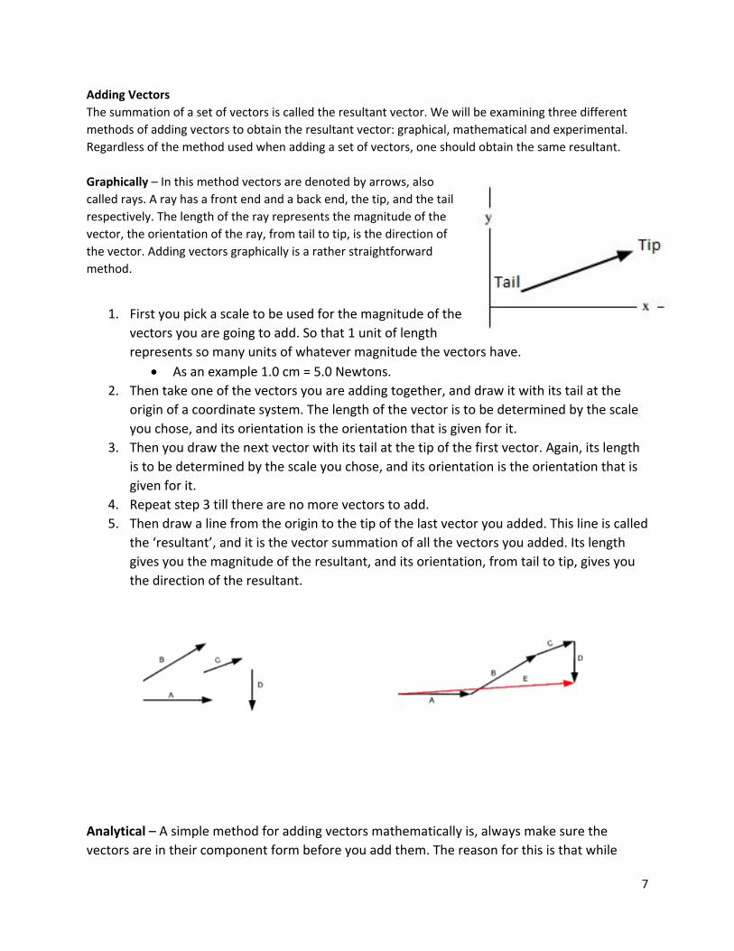
Graphically – In this method vectors are denoted by arrows, also 

called rays. A ray has a front end and a back end, the tip, and the tail 

respectively. The length of the ray represents the magnitude of the 

vector, the orientation of the ray, from tail to tip, is the direction of 

the vector. Adding vectors graphically is a rather straightforward 

method. 

 

1. First you pick a scale to be used for the magnitude of the 

vectors you are going to add. So that 1 unit of length 

represents so many units of whatever magnitude the vectors have.  

As an example 1.0 cm = 5.0 Newtons.  

2. Then take one of the vectors you are adding together, and draw it with its tail at the 

origin of a coordinate system. The length of the vector is to be determined by the scale 

you chose, and its orientation is the orientation that is given for it.  

3. Then you draw the next vector with its tail at the tip of the first vector. Again, its length 

is to be determined by the scale you chose, and its orientation is the orientation that is 

given for it. 

4. Repeat step 3 till there are no more vectors to add. 

5. Then draw a line from the origin to the tip of the last vector you added. This line is called 

the ‘resultant’, and it is the vector summation of all the vectors you added. Its length 

gives you the magnitude of the resultant, and its orientation, from tail to tip, gives you 

the direction of the resultant. 

   

 

 

 

 

  

 

Analytical – A simple method for adding vectors mathematically is, always make sure the 

vectors are in their component form before you add them. The reason for this is that while 

8  

adding vectors in their pure form can get rather complicated, vector components add like 

simple scalars. Meaning vector components obey the rules of simple arithmetic.  

 

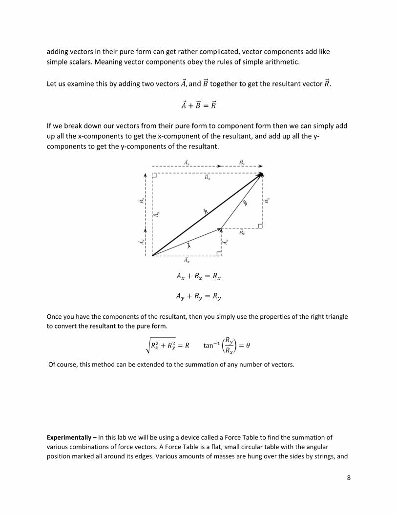
Let us examine this by adding two vectors 𝐴, and �⃗� together to get the resultant vector 𝑅. 

 

𝐴 �⃗� 𝑅 

 

If we break down our vectors from their pure form to component form then we can simply add 

up all the x‐components to get the x‐component of the resultant, and add up all the y‐

components to get the y‐components of the resultant. 

 

 

 

 

 

 

 

𝐴 𝐵 𝑅  

 

𝐴 𝐵 𝑅  

 Once you have the components of the resultant, then you simply use the properties of the right triangle 

to convert the resultant to the pure form. 

𝑅 𝑅 𝑅 tan𝑅𝑅

𝜃  

 Of course, this method can be extended to the summation of any number of vectors.  

 

 

 

 

Experimentally – In this lab we will be using a device called a Force Table to find the summation of 

various combinations of force vectors. A Force Table is a flat, small circular table with the angular 

position marked all around its edges. Various amounts of masses are hung over the sides by strings, and 

9  

those strings are all connected together by a little ring loop (or plastic ring) around a little pole at the 

center of the Force Table. To determine what the sum of all the force vectors the masses on the strings 

add up to, you add additional masses to yet another string till the new force balances out the original 

forces. When the forces are all balanced out, the loop ring will be right at the center of the Force Table. 

The force that balanced out the original forces is called the Equilibrant, and it made the entire system of 

forces sum to zero, because the Equilibrant has the exact same magnitude of the Resultant of the 

original forces, but the exact opposite direction. 

𝑅 𝑅, 𝜃 𝐸 𝑅, 𝜃 180  

PROCEDURE ‐ Experimental 

Part I:  Two Applied Forces 

1. Place a pulley at the 20.0o mark on the force table and place a total of 0.050 kg on the end of the string passing over this pulley.  Be sure to include the 0.005 kg of the mass holder in this total. Calculate the magnitude of the force (in Newtons) created by this mass. (Use three significant figures for all calculations in this laboratory.) Record the value of this force as F1 in Data Table 1. 

 

2. Place a second pulley at the 90.0o mark on the force table, using the same set of marks as the first.  Place a total of 0.100 kg on the end of the string.  Calculate the force produced and record as F2 in Data Table 1. 

 

3. Determine by trial and error where a third pulley must be located, with an appropriate mass, to set the connecting ring in equilibrium. This is achieved when the ring is centered over the pin. Assure that all strings are positioned on the ring so that each is directed toward the center of the ring. Move the ring off‐center and test if it returns to the desired location when released. 

 

4. Convert the mass determined in Step 3 to its force value, and record that value and direction (force table marker) as FE1, the equilibrant. 

 

5. From the value of the equilibrant force FE1, determine the magnitude and direction of the resultant force FR1, recording these two values in Data Table 1. 

 

Part II:  Three Applied Forces 

1. Place a pulley at 30.0o with 0.0500 kg on its string, one at 130.0o with 0.075 kg on it, and a third at 160.0o with 0.040 kg on it.  (Assure you are using the same set of degree marks.) 

 

2. Calculate the force produced by these three masses and record them as F3, F4, and F5 in Data Table 2. 

3. Following the procedure outlined in Steps 3 through 5 in Part I above, determine the equilibrant force and resultant force, recording their magnitudes and directions in Data Table 2 as FE2 and FR2. 

 

10  

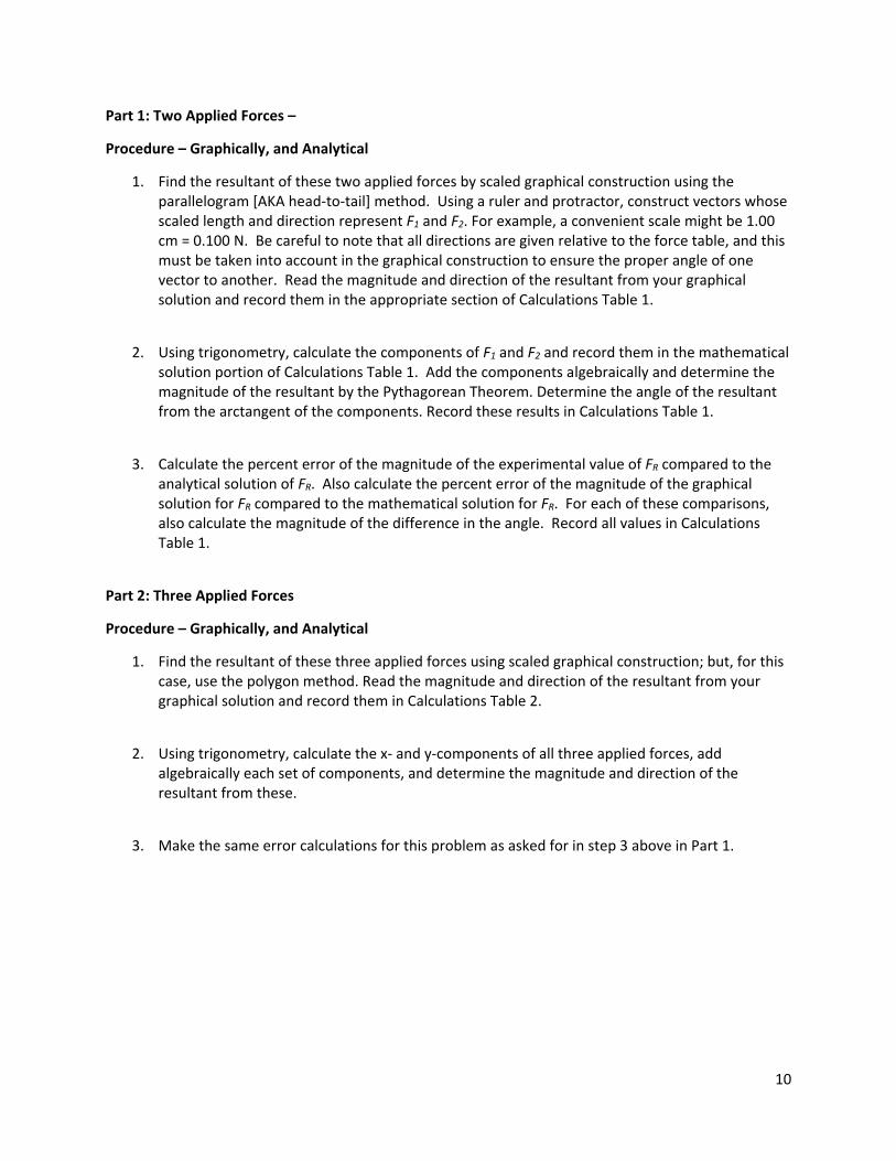
Part 1: Two Applied Forces –  

Procedure – Graphically, and Analytical  

1. Find the resultant of these two applied forces by scaled graphical construction using the parallelogram [AKA head‐to‐tail] method.  Using a ruler and protractor, construct vectors whose scaled length and direction represent F1 and F2. For example, a convenient scale might be 1.00 cm = 0.100 N.  Be careful to note that all directions are given relative to the force table, and this must be taken into account in the graphical construction to ensure the proper angle of one vector to another.  Read the magnitude and direction of the resultant from your graphical solution and record them in the appropriate section of Calculations Table 1. 

 

2. Using trigonometry, calculate the components of F1 and F2 and record them in the mathematical solution portion of Calculations Table 1.  Add the components algebraically and determine the magnitude of the resultant by the Pythagorean Theorem. Determine the angle of the resultant from the arctangent of the components. Record these results in Calculations Table 1. 

 

3. Calculate the percent error of the magnitude of the experimental value of FR compared to the analytical solution of FR.  Also calculate the percent error of the magnitude of the graphical solution for FR compared to the mathematical solution for FR.  For each of these comparisons, also calculate the magnitude of the difference in the angle.  Record all values in Calculations Table 1. 

 

Part 2: Three Applied Forces   

Procedure – Graphically, and Analytical 

1. Find the resultant of these three applied forces using scaled graphical construction; but, for this case, use the polygon method. Read the magnitude and direction of the resultant from your graphical solution and record them in Calculations Table 2.  

 

2. Using trigonometry, calculate the x‐ and y‐components of all three applied forces, add algebraically each set of components, and determine the magnitude and direction of the resultant from these. 

 

3. Make the same error calculations for this problem as asked for in step 3 above in Part 1.  

 

 

 

 

11  

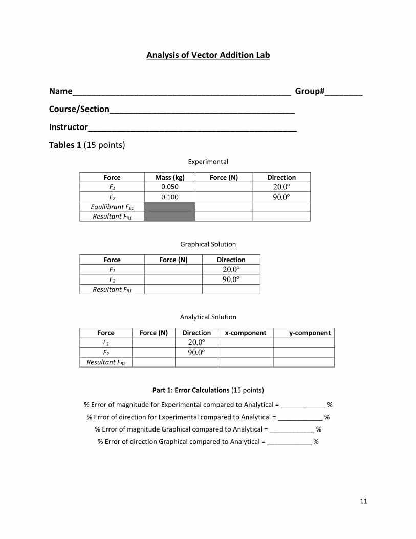
Analysis of Vector Addition Lab 

 

Name______________________________________________  Group#________ 

Course/Section_______________________________________ 

Instructor____________________________________________ 

Tables 1 (15 points) 

Experimental 

Force  Mass (kg)  Force (N)  Direction 

F1  0.050    0.20  

F2  0.100    0.90  

Equilibrant FE1       

Resultant FR1       

 

Graphical Solution 

Force  Force (N)  Direction 

F1    0.20  

F2    0.90  

Resultant FR1     

 

Analytical Solution 

Force  Force (N)  Direction  x‐component     y‐component 

F1    0.20      

F2    0.90      

Resultant FR2         

 

Part 1: Error Calculations (15 points) 

% Error of magnitude for Experimental compared to Analytical = ____________ % 

% Error of direction for Experimental compared to Analytical = ____________ % 

% Error of magnitude Graphical compared to Analytical = ____________ % 

% Error of direction Graphical compared to Analytical = ____________ % 

 

 

12  

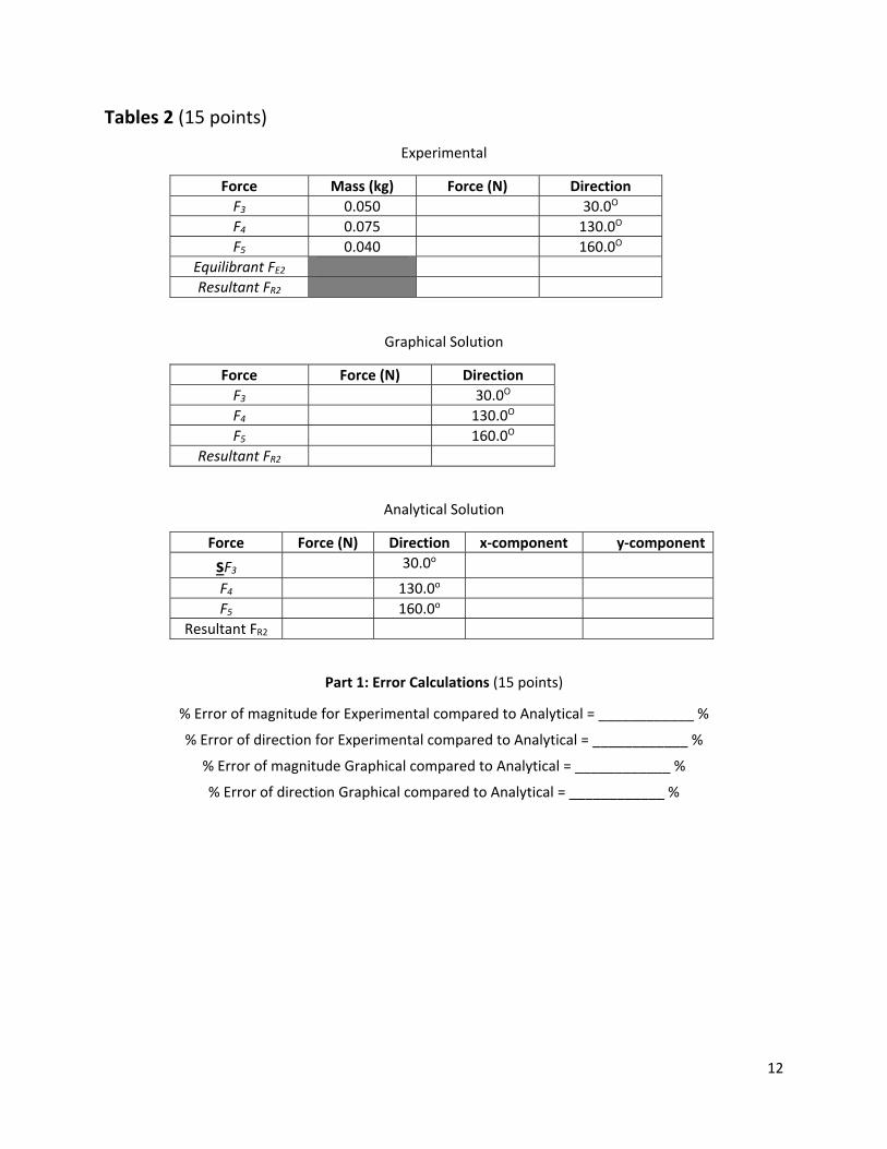
Tables 2 (15 points) 

Experimental 

Force  Mass (kg)  Force (N)  Direction 

F3  0.050    30.0O 

F4  0.075    130.0O 

F5  0.040    160.0O 

Equilibrant FE2       

Resultant FR2        

Graphical Solution 

Force  Force (N)  Direction 

F3    30.0O 

F4    130.0O 

F5    160.0O 

Resultant FR2     

 

Analytical Solution 

Force  Force (N)  Direction  x‐component     y‐component 

sF3    30.0o     

F4    130.0o     

F5    160.0o     

Resultant FR2         

 

Part 1: Error Calculations (15 points) 

% Error of magnitude for Experimental compared to Analytical = ____________ % 

% Error of direction for Experimental compared to Analytical = ____________ % 

% Error of magnitude Graphical compared to Analytical = ____________ % 

% Error of direction Graphical compared to Analytical = ____________ % 

 

 

 

 

 

 

13  

1. Possible sources of error include: (1) friction in the pulleys, (2) the strings actually have mass, and (3) errors in the direction of the forces if the strings do not act at 90O to a tangent to the ring. Based on the errors in your magnitude and direction calculations, rank the relative importance of these error sources for your data. (6 points) 

 

 

 

 

 

 

 

 

 

 

 

 

2. To determine the force acting in each mass, it was assumed that g = 9.80 m/s2. The value of g at the particular place where the experiment is performed may be slightly different from that value. State clearly what effect (if any) that variation would have on the percent error calculated for the components. In order to test your answer to the question, leave g as a symbol in the calculation of the percent error. (6 points) 

 

 

 

 

 

 

 

 

 

 

 

14  

3. Two forces are applied to the ring of a force table, one at an angle of 0.20 , and the other at

0.80 . Regardless of the magnitude of the forces, will the equilibrant be in the (a) first quadrant, (b) second quadrant, (c) third quadrant, (d) fourth quadrant or (e) you cannot tell which quadrant from the available information? (8 points) 

 

 

 

 

 

 

 

4. Two forces, one of magnitude 2.00 N and the other of magnitude 3.00 N, are applied to the ring of a force table. The directions of both forces are unknown. Which best describes the limitations on the magnitude of R, the resultant? (8 points) 

(a)  NR 5  (b) NRN 32  (c) NR 3 (d)  NRN 51  (e) NR 2  

 

 

 

 

 

 

5. Suppose the same masses are used for a force table experiment as were used in Part 1, but each 

pulley is moved  180 so that the 0.050 kg mass acts at  200 , and the 0.100 kg mass acts at 

270 .  What is the magnitude of the resultant in this case? How does it compare to the resultant in Part 1? (6 points) 

 

 

 

 

 

 

 

 

15  

 

6. As stated earlier, the pulleys introduce a possible source of error because of their possible friction. Given that they are a source of error, why are the pulleys used at all? In other words, what is the function of the pulleys? (6 points)