xPSD: An External Solver To Compute Linear Responses To Random Base Excitations (PSD) In

Structures Using ANSYS With The Large Mass Method Alex Grishin Matt Sutton

Phoenix Analysis And Design Technologies, Inc. Abstract It is sometimes desirable to incorporate one's own solver with a finite element model created using commercial finite element software. ANSYS facilitates such efforts through the use of User-Defined Features [3] (UDF's) and the ANSYS Application Programmers Interface (API). This paper summarizes one such application developed by the authors for a customer with very specific needs in the calculation of structural response to random base excitations. The software solution described in this report differs substantially with the PSD random vibration solver offered by ANSYS Inc. in several respects - both in theoretical approach taken and program architecture. The net result offers the user a reduction in computer storage requirements and calculation speed for the analysis of structures subjected to a single random base excitation.

Introduction Phoenix Analysis and Design Technologies (PADT) was approached by a large corporate defense contractor regarding specific needs they had when using ANSYS to analyze the structural response of their products to random base excitations, represented in the form of Power Spectral Density (PSD) curves. The customer wanted to create their FE models using ANSYS’s substantial element library and preprocessing tools but had the following requirements of the random vibration solution:

1. All model databases should be relatively small (preferably never exceeding the 2 GB range for even their largest models).

2. All model databases should be static and load independent (for a given model and constraints, a user should be able to run several different load cases without changing the databases - i.e. without substantial disk i/o - and without re-extracting Eigenquantities).

3. The users experience was determined to be predominantly shaped by program runtimes, therefore, any random vibration result must be computed as expediently as possible. Preferably, all computations should require 60 sec or less for reasonably large models running on standard workstation hardware.

The customer based these requirements on their experience with another leading software package. Since the customer rarely considers multiple simultaneous base excitations and/or nodal excitations (in such cases, the company would employ ANSYS's current random vibration solver), the company's goals were considered reasonable if the authors could develop an external program which would employ mode superposition (mode displacement method) with the Large Mass Method for base excitations - the fastest and simplest method known - and known to be used by the competitor.

With this method, it was clear that the only persistent quantities required (in addition to the model DB) were the eigenquantities and eigenvalues (natural frequencies). Linking an external program written in C++ with ANSYS’s C API would create these databases. It can then be invoked on the ANSYS command line as a tilde (~) command. Two other completely external components would be created to complete the authors' solution. The combined suite of software components is called xPSD.

The Large Mass Method (LMM) By application of the Large Mass Method (LMM), the analyst attempts to simulate a base excitation by coupling a large mass element to the degrees of freedom which make up the base of the structure and applying a force equal to Mω2x, where M is the actual mass, ω is the frequency of the harmonic load, and x is the amplitude of base excitation. Since the load is a base excitation, x is usually known and F is solved. This is an approximation which can only be justified when M is very large compared with the mass of the structure. An informal explanation of this is as follows:

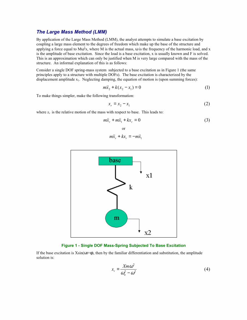
Consider a single DOF spring-mass system subjected to a base excitation as in Figure 1 (the same principles apply to a structure with multiple DOFs). The base excitation is characterized by the displacement amplitude x1. Neglecting damping, the equation of motion is (upon summing forces):

)1(0)( 122 =−+ xxkxm &&

To make things simpler, make the following transformation:

)2(12 xxxr −=

where xr is the relative motion of the mass with respect to base. This leads to:

)3(01 =++ rr kxxmxm &&&&

or

1xmkxxm rr &&&& −=+

Figure 1 - Single DOF Mass-Spring Subjected To Base Excitation

If the base excitation is Xsin(ωt+φ), then by the familiar differentiation and substitution, the amplitude solution is:

)4(22

2

ωωω

−=

nr

Xmx

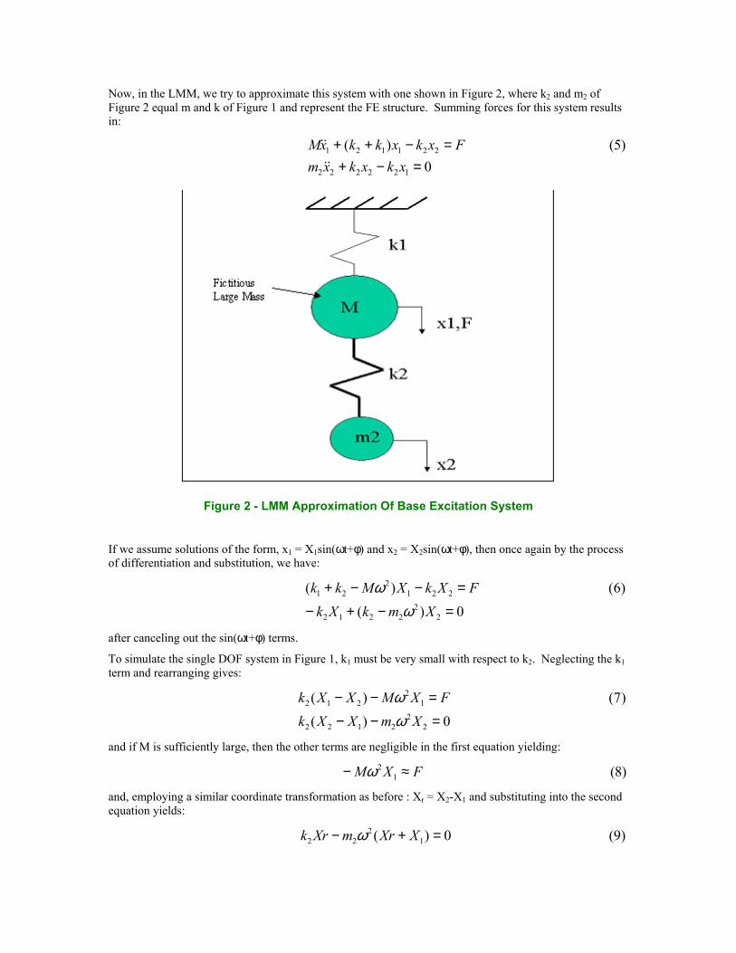
Now, in the LMM, we try to approximate this system with one shown in Figure 2, where k2 and m2 of Figure 2 equal m and k of Figure 1 and represent the FE structure. Summing forces for this system results in:

0)5()(

122222

221121

=−+=−++

xkxkxmFxkxkkxM

&&

&&

Figure 2 - LMM Approximation Of Base Excitation System

If we assume solutions of the form, x1 = X1sin(ωt+φ) and x2 = X2sin(ωt+φ), then once again by the process of differentiation and substitution, we have:

0)(

)6()(

22

2212

2212

21

=−+−

=−−+

XmkXkFXkXMkk

ωω

after canceling out the sin(ωt+φ) terms.

To simulate the single DOF system in Figure 1, k1 must be very small with respect to k2. Neglecting the k1 term and rearranging gives:

0)(

)7()(

22

2122

12

212

=−−

=−−

XmXXkFXMXXk

ωω

and if M is sufficiently large, then the other terms are negligible in the first equation yielding:

)8(12 FXM ≈− ω

and, employing a similar coordinate transformation as before : Xr = X2-X1 and substituting into the second equation yields:

)9(0)( 12

22 =+− XXrmXrk ω

or

221

222 ωω mXXrmXrk =−

which yields approximately the same solution as (1):

)10(22

221

ωωω

−≈

n

mXXr

This solution is approximate because the displacement amplitude X1 is obtained from the approximation:

)11(21 ωMFX ≈

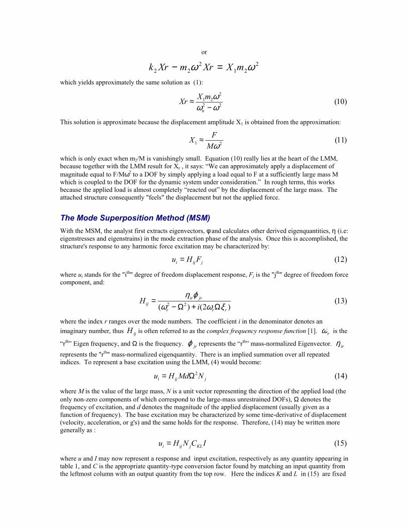
which is only exact when m2/M is vanishingly small. Equation (10) really lies at the heart of the LMM, because together with the LMM result for Xr , it says: “We can approximately apply a displacement of magnitude equal to F/Mω2 to a DOF by simply applying a load equal to F at a sufficiently large mass M which is coupled to the DOF for the dynamic system under consideration.” In rough terms, this works because the applied load is almost completely “reacted out” by the displacement of the large mass. The attached structure consequently "feels" the displacement but not the applied force.

The Mode Superposition Method (MSM) With the MSM, the analyst first extracts eigenvectors, φ and calculates other derived eigenquantities, η (i.e: eigenstresses and eigenstrains) in the mode extraction phase of the analysis. Once this is accomplished, the structure's response to any harmonic force excitation may be characterized by:

)12(jiji FHu =

where ui stands for the "ith" degree of freedom displacement response, Fj is the "jth" degree of freedom force component, and:

)13()2()( 22

rrr

jririj i

Hξωω

ϕηΩ+Ω−

=

where the index r ranges over the mode numbers. The coefficient i in the denominator denotes an imaginary number, thus is often referred to as the complex frequency response function [1]. ijH rω is the

“rth” Eigen frequency, and Ω is the frequency. jrϕ represents the “rth” mass-normalized Eigenvector. irη represents the "rth" mass-normalized eigenquantity. There is an implied summation over all repeated indices. To represent a base excitation using the LMM, (4) would become:

)14(2jiji NMdHu Ω=

where M is the value of the large mass, N is a unit vector representing the direction of the applied load (the only non-zero components of which correspond to the large-mass unrestrained DOFs), Ω denotes the frequency of excitation, and d denotes the magnitude of the applied displacement (usually given as a function of frequency). The base excitation may be characterized by some time-derivative of displacement (velocity, acceleration, or g's) and the same holds for the response. Therefore, (14) may be written more generally as :

)15(ICNHu KLjiji =

where u and I may now represent a response and input excitation, respectively as any quantity appearing in table 1, and C is the appropriate quantity-type conversion factor found by matching an input quantity from the leftmost column with an output quantity from the top row. Here the indices K and L in (15) are fixed

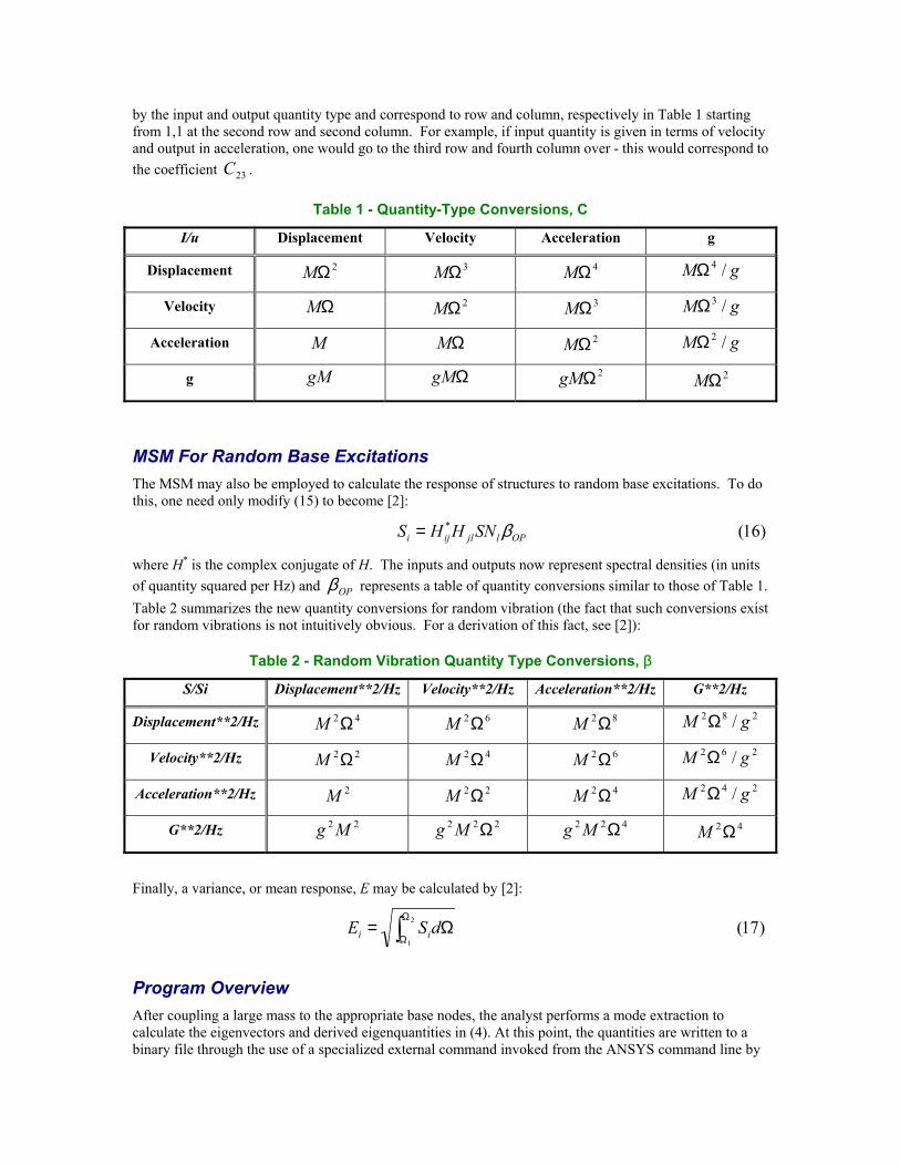
by the input and output quantity type and correspond to row and column, respectively in Table 1 starting from 1,1 at the second row and second column. For example, if input quantity is given in terms of velocity and output in acceleration, one would go to the third row and fourth column over - this would correspond to the coefficient C . 23

Table 1 - Quantity-Type Conversions, C

I/u Displacement Velocity Acceleration g

Displacement 2ΩM 3ΩM 4ΩM gM /4Ω

Velocity ΩM 2ΩM 3ΩM gM /3Ω

Acceleration M ΩM 2ΩM gM /2Ω

g gM ΩgM 2ΩgM 2ΩM

MSM For Random Base Excitations The MSM may also be employed to calculate the response of structures to random base excitations. To do this, one need only modify (15) to become [2]:

)16(*OPljliji SNHHS β=

where H* is the complex conjugate of H. The inputs and outputs now represent spectral densities (in units of quantity squared per Hz) and OPβ represents a table of quantity conversions similar to those of Table 1. Table 2 summarizes the new quantity conversions for random vibration (the fact that such conversions exist for random vibrations is not intuitively obvious. For a derivation of this fact, see [2]):

Table 2 - Random Vibration Quantity Type Conversions, β

S/Si Displacement**2/Hz Velocity**2/Hz Acceleration**2/Hz G**2/Hz

Displacement**2/Hz 42ΩM 62ΩM

82ΩM 282 / gM Ω

Velocity**2/Hz 22ΩM 42ΩM

62ΩM 262 / gM Ω

Acceleration**2/Hz 2M 22ΩM

42ΩM 242 / gM Ω

G**2/Hz 22Mg 222 ΩMg

422 ΩMg 42ΩM

Finally, a variance, or mean response, E may be calculated by [2]:

)17(2

1

Ω= ∫Ω

ΩdSE ii

Program Overview After coupling a large mass to the appropriate base nodes, the analyst performs a mode extraction to calculate the eigenvectors and derived eigenquantities in (4). At this point, the quantities are written to a binary file through the use of a specialized external command invoked from the ANSYS command line by

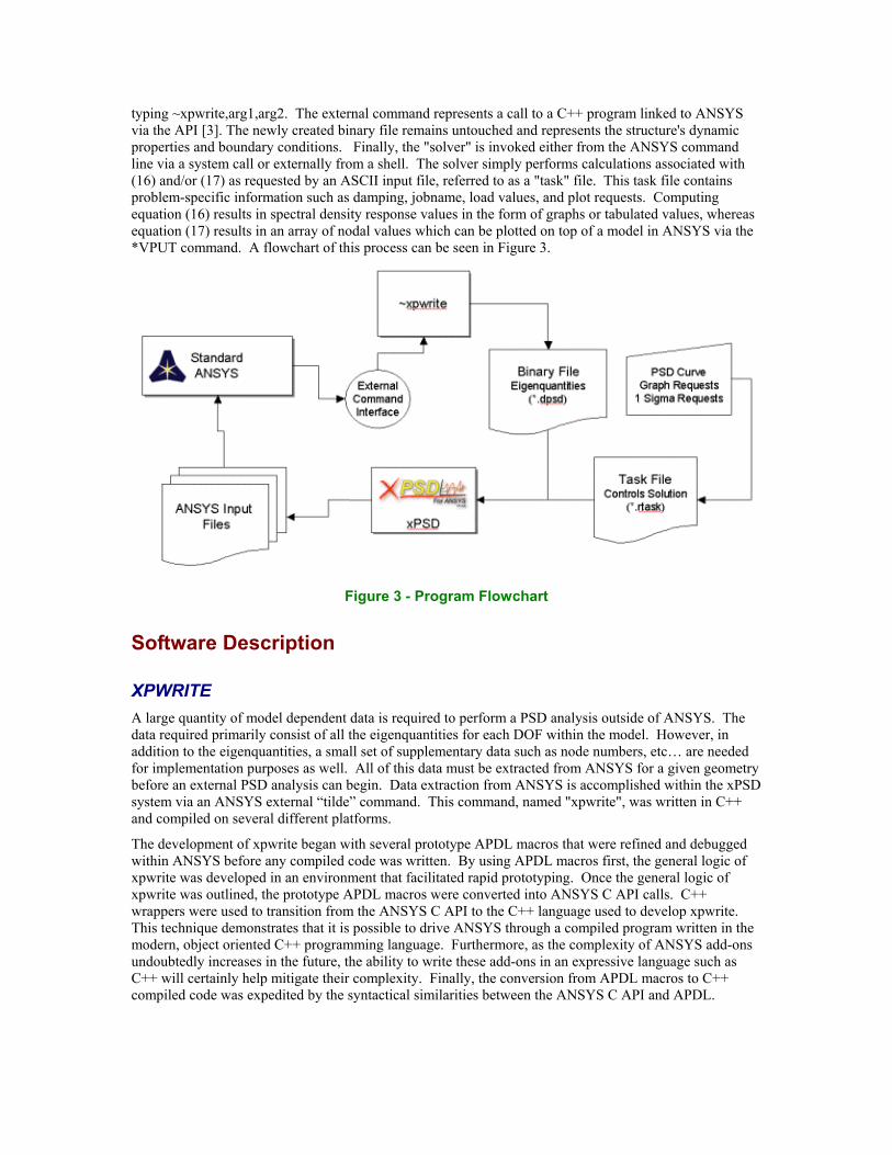
typing ~xpwrite,arg1,arg2. The external command represents a call to a C++ program linked to ANSYS via the API [3]. The newly created binary file remains untouched and represents the structure's dynamic properties and boundary conditions. Finally, the "solver" is invoked either from the ANSYS command line via a system call or externally from a shell. The solver simply performs calculations associated with (16) and/or (17) as requested by an ASCII input file, referred to as a "task" file. This task file contains problem-specific information such as damping, jobname, load values, and plot requests. Computing equation (16) results in spectral density response values in the form of graphs or tabulated values, whereas equation (17) results in an array of nodal values which can be plotted on top of a model in ANSYS via the *VPUT command. A flowchart of this process can be seen in Figure 3.

Figure 3 - Program Flowchart

Software Description

XPWRITE A large quantity of model dependent data is required to perform a PSD analysis outside of ANSYS. The data required primarily consist of all the eigenquantities for each DOF within the model. However, in addition to the eigenquantities, a small set of supplementary data such as node numbers, etc… are needed for implementation purposes as well. All of this data must be extracted from ANSYS for a given geometry before an external PSD analysis can begin. Data extraction from ANSYS is accomplished within the xPSD system via an ANSYS external “tilde” command. This command, named "xpwrite", was written in C++ and compiled on several different platforms.

The development of xpwrite began with several prototype APDL macros that were refined and debugged within ANSYS before any compiled code was written. By using APDL macros first, the general logic of xpwrite was developed in an environment that facilitated rapid prototyping. Once the general logic of xpwrite was outlined, the prototype APDL macros were converted into ANSYS C API calls. C++ wrappers were used to transition from the ANSYS C API to the C++ language used to develop xpwrite. This technique demonstrates that it is possible to drive ANSYS through a compiled program written in the modern, object oriented C++ programming language. Furthermore, as the complexity of ANSYS add-ons undoubtedly increases in the future, the ability to write these add-ons in an expressive language such as C++ will certainly help mitigate their complexity. Finally, the conversion from APDL macros to C++ compiled code was expedited by the syntactical similarities between the ANSYS C API and APDL.

The Internal Structure of XPWRITE Internally, xpwrite adheres to an object-oriented, modular design philosophy. There are two main objects within xpwrite that collaborate to provide the total functionality for the command. The first object is designed to interface with ANSYS through the ANSYS C API and provide all of the data querying functionality necessary to extract the eigenquantities, etc… from ANSYS. The second object is designed to interface with the modal database and provide read/write capabilities to and from the database. During the execution of the command, the first object queries ANSYS and feeds the resulting data to the second object through a simple interface. Since the mechanics of reading and writing to the binary database are hidden behind a simple interface, changes to the database structure and read/write mechanisms can be made without affecting the object responsible for querying ANSYS. Likewise, the methods used to query ANSYS are hidden behind a separate simple interface, and therefore, they too can be altered without jeopardizing the functionality of the database object.

Eigenquantity Binary Database In order to perform a PSD analysis for a given model outside of ANSYS using an external PSD solver, all the eigenquantities for the model must be available for consumption by the external solver. Consequently, within the xPSD system, all the eigenquanitites, along with a small quantity of additional data, are stored in a binary database. Several requirements were imposed on the design of the binary database:

1. Random access was required to be performed in constant time.

2. The database was required to be platform independent.

3. File size was required to be kept to a minimum.

As in most designs, each one of the requirements mentioned above is interdependent. For example, constant time random access conflicts with both minimal file size, and platform independence. Because of these conflicts, the requirements were weighed based on their perceived importance to the user’s experience and then sorted based on their weights. It was determined that the most important user experience would be computational speed and platform independence. Therefore, the binary database design gave precedence to platform independence and random access time at the expense of file size. In the future, however, in-stream compression techniques may be explored as possible alternative implementations that would reduce the file size, yet still maintain acceptable access times and platform independence.

The Task File In its current form, xPSD is designed to be used as a batch tool. As such, the program reads instructions for what tasks to perform from a free format ASCII text file. In addition to storing the task commands (Commands are written as keywords preceded by asterisks, followed by arguments), this file also stores all loading information, as well as critical damping ratio, job name, and the value of g (acceleration due to gravity). In this way, multiple load cases may be stored as separate task files - each containing a unique job name. At present, the user must create this file manually, but PADT has plans to implement a graphical user interface, which would produce the task file as an echoed hardcopy of the user's interface picks - similar to an ANSYS log file. An example task file with annotations is shown in Figure 4.

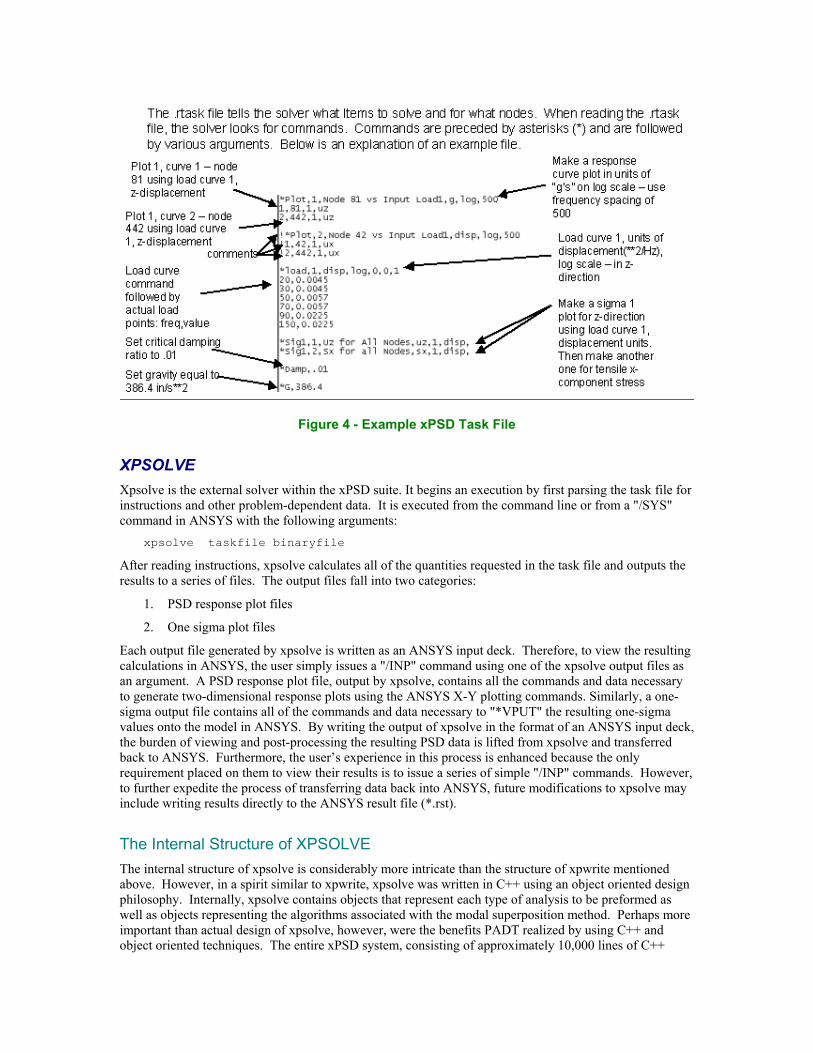
Figure 4 - Example xPSD Task File

XPSOLVE Xpsolve is the external solver within the xPSD suite. It begins an execution by first parsing the task file for instructions and other problem-dependent data. It is executed from the command line or from a "/SYS" command in ANSYS with the following arguments:

xpsolve taskfile binaryfile

After reading instructions, xpsolve calculates all of the quantities requested in the task file and outputs the results to a series of files. The output files fall into two categories:

1. PSD response plot files

2. One sigma plot files

Each output file generated by xpsolve is written as an ANSYS input deck. Therefore, to view the resulting calculations in ANSYS, the user simply issues a "/INP" command using one of the xpsolve output files as an argument. A PSD response plot file, output by xpsolve, contains all the commands and data necessary to generate two-dimensional response plots using the ANSYS X-Y plotting commands. Similarly, a one-sigma output file contains all of the commands and data necessary to "*VPUT" the resulting one-sigma values onto the model in ANSYS. By writing the output of xpsolve in the format of an ANSYS input deck, the burden of viewing and post-processing the resulting PSD data is lifted from xpsolve and transferred back to ANSYS. Furthermore, the user’s experience in this process is enhanced because the only requirement placed on them to view their results is to issue a series of simple "/INP" commands. However, to further expedite the process of transferring data back into ANSYS, future modifications to xpsolve may include writing results directly to the ANSYS result file (*.rst).

The Internal Structure of XPSOLVE The internal structure of xpsolve is considerably more intricate than the structure of xpwrite mentioned above. However, in a spirit similar to xpwrite, xpsolve was written in C++ using an object oriented design philosophy. Internally, xpsolve contains objects that represent each type of analysis to be preformed as well as objects representing the algorithms associated with the modal superposition method. Perhaps more important than actual design of xpsolve, however, were the benefits PADT realized by using C++ and object oriented techniques. The entire xPSD system, consisting of approximately 10,000 lines of C++

code, was conceived and written in 20 workdays by two individuals. This was accomplished by maximizing the use of pre-existing, high quality libraries such as the Standard Template Library throughout the design. By offloading the tedious and error prone programming chores associated with general data structure design to pre-existing template libraries, PADT realized a substantial increase in productivity and code robustness. Furthermore, by judiciously subdividing the problem into objects and their relationships, the complexity associated with the xPSD system as a whole was reduced.

Examples PADT has used xPSD for consulting work and has performed benchmark testing on several FE models representing real-world structures. The benchmarks consisted of comparing the run-times between xPSD and the ANSYS Random Vibration Solver as well as the differences between result quantities between the two solvers for given loading conditions.

Run-Time Comparisons Of all models tested, those summarized in Table 3 showed the most significant differences in run-times (these were some of the larger models tested). Significant reductions in run-time were realized for problems involving a single base-excitation, as can be seen in Table 4. It should be noted that, in calculating the variance (the one-sigma values), ANSYS calculates all quantities, whereas xPSD only calculates those quantities requested by the user. The xPSD variance calculation times reflect the time required to calculate 13 quantities - the component displacements, six stress components, three principle stresses, and an equivalent stress. xPSD does not currently support the calculation of strain values, as the customer expresses no interest in one-sigma strain values but the reader should note that their calculation would almost double the variance calculation times. Consequently, the values in the third column of Table 4 should be multiplied by a factor of two for a more accurate comparison of calculation times. The graph calculation times (second and fourth columns, respectively), reflect the time it took both ANSYS and xPSD to calculate and return power spectral density results for the frequency range of the input load curve. For cases 2 through 4, the power spectral density response at two nodes for all load frequencies comprises one graph. For case 1, the response for six nodes for all load frequencies comprises one graph. All benchmark run-times were obtained on a desktop PC with dual Pentium III processors with 1000 Mhertz clockspeeds and 1.5 Gigabytes of RAM.

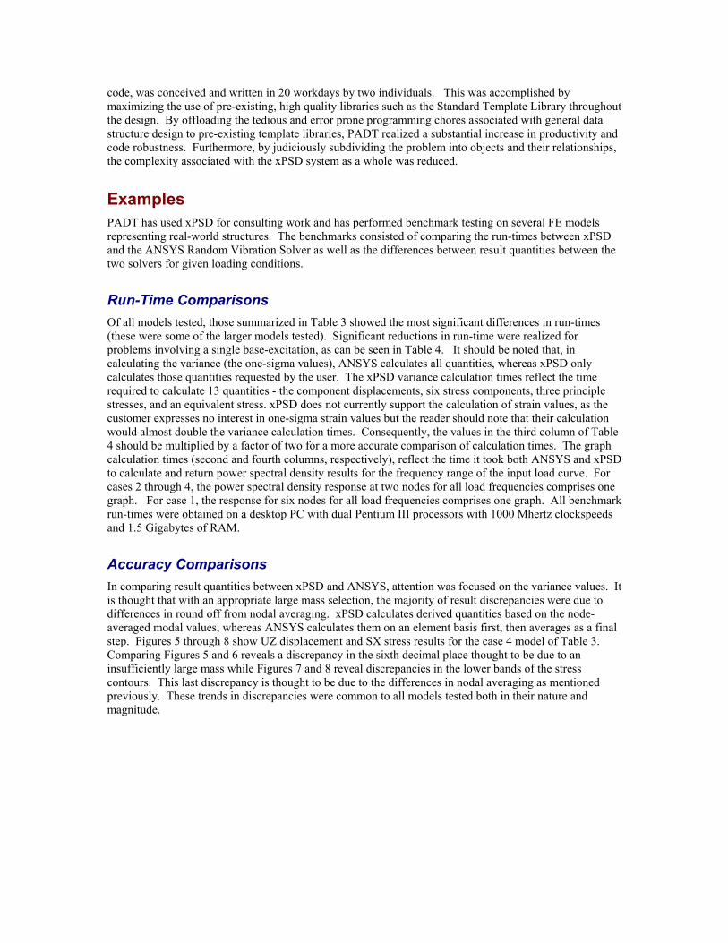
Accuracy Comparisons In comparing result quantities between xPSD and ANSYS, attention was focused on the variance values. It is thought that with an appropriate large mass selection, the majority of result discrepancies were due to differences in round off from nodal averaging. xPSD calculates derived quantities based on the node-averaged modal values, whereas ANSYS calculates them on an element basis first, then averages as a final step. Figures 5 through 8 show UZ displacement and SX stress results for the case 4 model of Table 3. Comparing Figures 5 and 6 reveals a discrepancy in the sixth decimal place thought to be due to an insufficiently large mass while Figures 7 and 8 reveal discrepancies in the lower bands of the stress contours. This last discrepancy is thought to be due to the differences in nodal averaging as mentioned previously. These trends in discrepancies were common to all models tested both in their nature and magnitude.

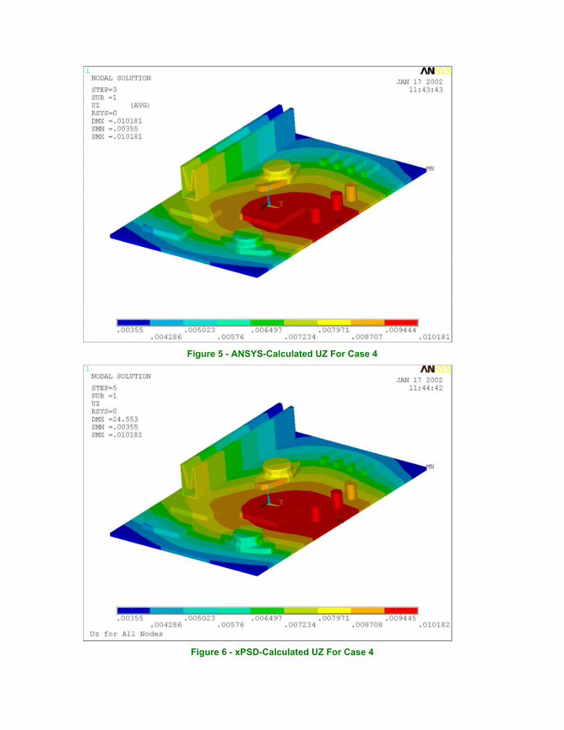
Figure 5 - ANSYS-Calculated UZ For Case 4

Figure 6 - xPSD-Calculated UZ For Case 4

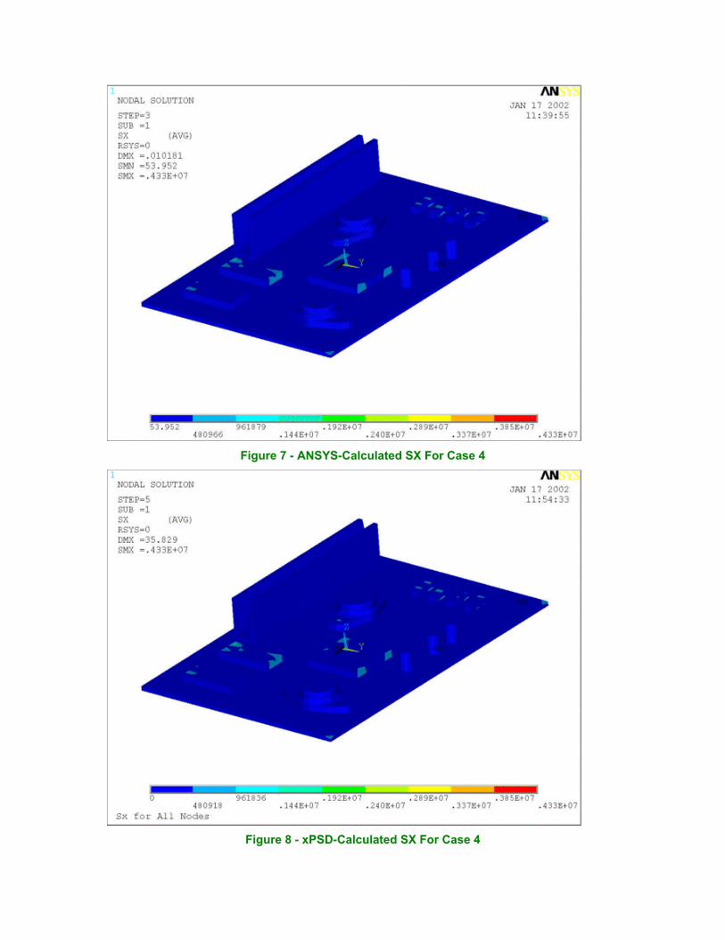
Figure 7 - ANSYS-Calculated SX For Case 4

Figure 8 - xPSD-Calculated SX For Case 4

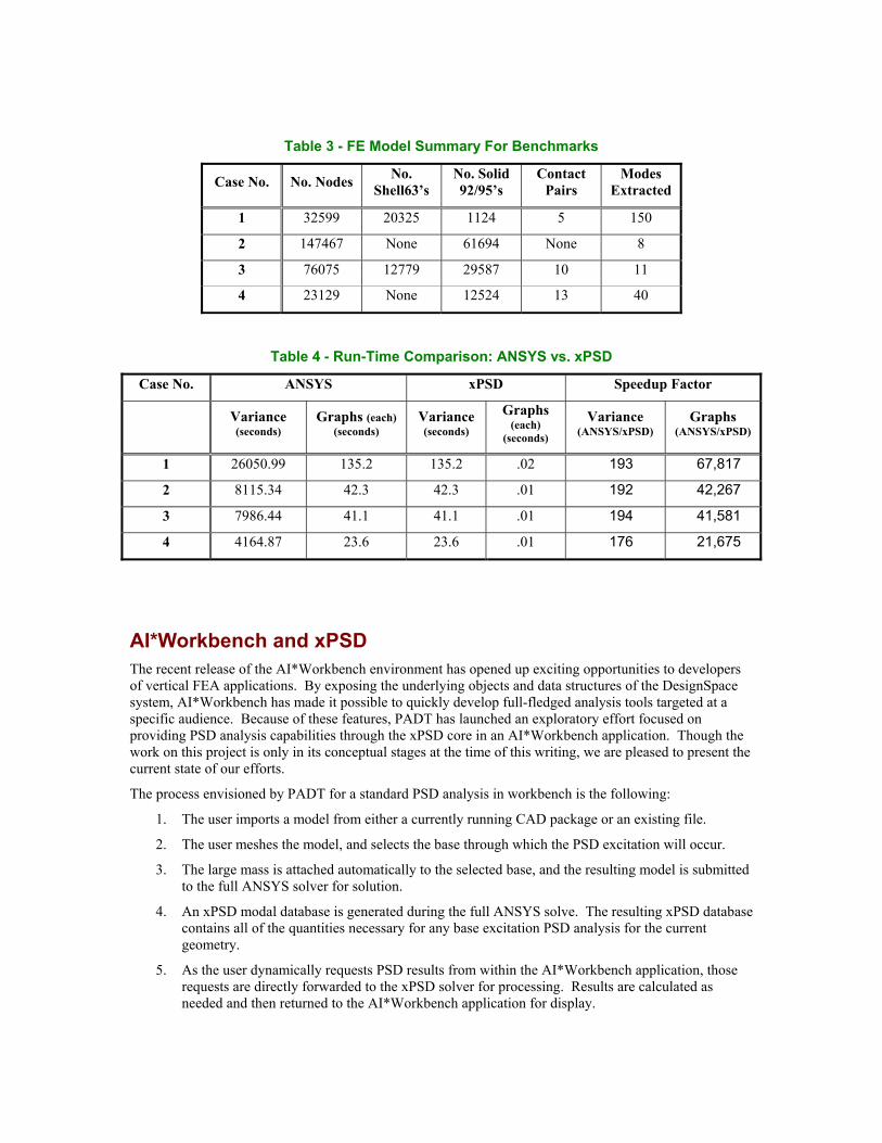
Table 3 - FE Model Summary For Benchmarks

Case No. No. Nodes No. Shell63’s

No. Solid 92/95’s

Contact Pairs

Modes Extracted

1 32599 20325 1124 5 150

2 147467 None 61694 None 8

3 76075 12779 29587 10 11

4 23129 None 12524 13 40

Table 4 - Run-Time Comparison: ANSYS vs. xPSD

Case No. ANSYS xPSD Speedup Factor

Variance (seconds)

Graphs (each) (seconds)

Variance (seconds)

Graphs (each)

(seconds) Variance

(ANSYS/xPSD) Graphs

(ANSYS/xPSD)

1 26050.99 135.2 135.2 .02 193 67,817

2 8115.34 42.3 42.3 .01 192 42,267

3 7986.44 41.1 41.1 .01 194 41,581

4 4164.87 23.6 23.6 .01 176 21,675

AI*Workbench and xPSD The recent release of the AI*Workbench environment has opened up exciting opportunities to developers of vertical FEA applications. By exposing the underlying objects and data structures of the DesignSpace system, AI*Workbench has made it possible to quickly develop full-fledged analysis tools targeted at a specific audience. Because of these features, PADT has launched an exploratory effort focused on providing PSD analysis capabilities through the xPSD core in an AI*Workbench application. Though the work on this project is only in its conceptual stages at the time of this writing, we are pleased to present the current state of our efforts.

The process envisioned by PADT for a standard PSD analysis in workbench is the following:

1. The user imports a model from either a currently running CAD package or an existing file.

2. The user meshes the model, and selects the base through which the PSD excitation will occur.

3. The large mass is attached automatically to the selected base, and the resulting model is submitted to the full ANSYS solver for solution.

4. An xPSD modal database is generated during the full ANSYS solve. The resulting xPSD database contains all of the quantities necessary for any base excitation PSD analysis for the current geometry.

5. As the user dynamically requests PSD results from within the AI*Workbench application, those requests are directly forwarded to the xPSD solver for processing. Results are calculated as needed and then returned to the AI*Workbench application for display.

Steps 1 through 4 listed above are fairly standard AI*Workbench development procedures and they mimick the steps used for the ANSYS version of xPSD. The deviation from standard AI*Workbench applications occurs primarily in step 5. Therefore, the following discussion and screen captures focus on the user’s experience in step 5 alone.

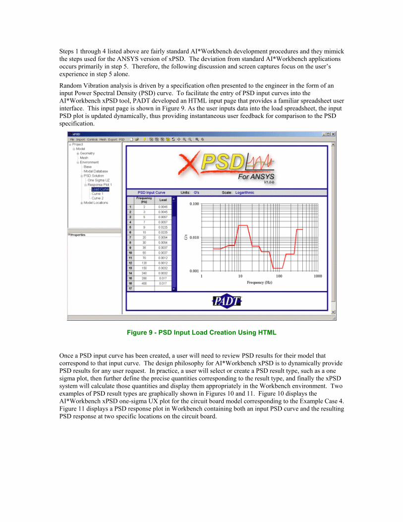
Random Vibration analysis is driven by a specification often presented to the engineer in the form of an input Power Spectral Density (PSD) curve. To facilitate the entry of PSD input curves into the AI*Workbench xPSD tool, PADT developed an HTML input page that provides a familiar spreadsheet user interface. This input page is shown in Figure 9. As the user inputs data into the load spreadsheet, the input PSD plot is updated dynamically, thus providing instantaneous user feedback for comparison to the PSD specification.

Figure 9 - PSD Input Load Creation Using HTML

Once a PSD input curve has been created, a user will need to review PSD results for their model that correspond to that input curve. The design philosophy for AI*Workbench xPSD is to dynamically provide PSD results for any user request. In practice, a user will select or create a PSD result type, such as a one sigma plot, then further define the precise quantities corresponding to the result type, and finally the xPSD system will calculate those quantities and display them appropriately in the Workbench environment. Two examples of PSD result types are graphically shown in Figures 10 and 11. Figure 10 displays the AI*Workbench xPSD one-sigma UX plot for the circuit board model corresponding to the Example Case 4. Figure 11 displays a PSD response plot in Workbench containing both an input PSD curve and the resulting PSD response at two specific locations on the circuit board.

Figure 10 - xPSD SX Result In AI*Workbench

Figure 11 - xPSD Nodal Response Curve In AI*Workbench

After completing the initial stages of development presented here, PADT is confident that a viable AI*Workbench based PSD analysis tool can be created to leverage the user’s understanding of their products and needs while taking advantage of the computational speed of the xPSD core, the element and solver technology of the full ANSYS solver, and the pre and post processing strengths of the AI*Workbench environment.

Conclusion Although this project was carried out to address a specific need of a specific customer, it serves as an example of the flexibility and openness of the ANSYS product. With a limited budget and an even more limited schedule, it was necessary to use as much existing functionality and code as possible. The ANSYS command language and the ‘C’ API allowed the development team to use ANSYS’s inherent strengths while only adding the functionality that was needed. In addition, the use of an objected oriented approach with C++ allowed the team to reuse a considerable amount of code for data storage, extraction and manipulation. The amount of time and resources spent on this project was a fraction of what would have required to write a completely stand alone program.

In the end, PADT was able to deliver a significant increase in productivity and efficiency within 20 working days utilizing two part time developers. Also, the resulting tool is modular enough to allow it to also be included in an AI*Workbench based tool or to be expanded into a solver for other dynamic analyses such as forced vibration, harmonics or modal superposition.

References 1. Craig, Roy R. Jr., Structural Dynamics: An Introduction to Computer Methods, John Wiley &

Sons, 1981, New York

2. Newland, D.E., An Introduction to Random Vibration and Spectral Analysis, Longman Group, Ltd., 1975, London

3. ANSYS Programmer's Manual - User Programmable Features