20. compilerscompalg.inf.elte.hu/~tony/informatikai-konyvtar/03... · 2006-05-29 · the task of...

20. Compilers

When a programmer writes down a solution of her problems, she writes a program on aspecial programming language. These programming languages are very different from theproper languages of computers, from the machine languages. Therefore we have to pro-duce the executable forms of programs created by the programmer. We need a softwareor hardware tool, that translates the source language program � written on a high levelprogramming language � to the target language program, a lower level programming lan-guage, mostly to a machine code program.

There are two fundamental methods to execute a program written on higher level lan-guage. The �rst is using an interpreter. In this case, the generated machine code is notsaved but executed immediately. The interpreter is considered as a special computer, whosemachine code is the high level language. Essentially, when we use an interpreter, then wecreate a two-level machine; its lower level is the real computer, on which the higher level,the interpreter, is built. The higher level is usually realized by a computer program, but, forsome programming languages, there are special hardware interpreter machines.

The second method is using a compiler program. The difference of this method fromthe �rst is that here the result of translation is not executed, but it is saved in an intermediate�le called target program.

The target program may be executed later, and the result of the program is receivedonly then. In this case, in contrast with interpreters, the times of translation and executionare distinguishable.

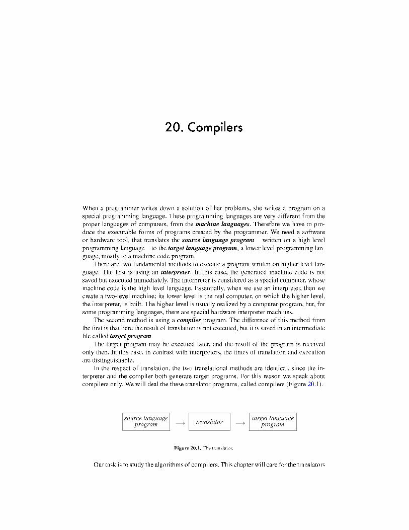
In the respect of translation, the two translational methods are identical, since the in-terpreter and the compiler both generate target programs. For this reason we speak aboutcompilers only. We will deal the these translator programs, called compilers (Figure 20.1).

translatorsource languageprogram

target languageprogram−→ −→

Figure 20.1. The translator.

Our task is to study the algorithms of compilers. This chapter will care for the translators

952 20. Compilers

of high level imperative programming languages; the translational methods of logical orfunctional languages will not be investigated.

First the structure of compilers will be given. Then we will deal with scanners, that is,lexical analysers. In the topic of parsers � syntactic analysers �, the two most successful met-hods will be studied: the LL(1) and the LALR(1) parsing methods. The advanced methodsof semantic analysis use O-ATG grammars, and the task of code generation is also writtenby this type of grammars. In this book these topics are not considered, nor we will studysuch important and interesting problems as symbol table handling, error repairing or codeoptimising. The reader can �nd very new, modern and efficient methods for these methodsin the bibliography.

20.1. The structure of compilersA compiler translates the source language program (in short, source program) into a tar-get language program (in short, target program). Moreover, it creates a list by which theprogrammer can check her private program. This list contains the detected errors, too.

Using the notation program (input)(output) the compiler can be written by

compiler (source program)(target program, list).

In the next, the structure of compilers are studied, and the tasks of program elements aredescribed, using the previous notation.

The �rst program of a compiler transforms the source language program into characterstream that is easy to handle. This program is the source handler.

source handler (source program)(character stream).

The form of the source program depends from the operating system. The source handlerreads the �le of source program using a system, called operating system, and omits thecharacters signed the end of lines, since these characters have no importance in the nextsteps of compilation. This modi�ed, �poured� character stream will be the input data of thenext steps.

The list created by the compiler has to contain the original source language programwritten by the programmer, instead of this modi�ed character stream. Hence we de�ne a listhandler program,

list handler (source program, errors)(list),

which creates the list according to the �le form of the operating system, and puts this list ona secondary memory.

It is practical to join the source handler and the list handler programs, since they havesame input �les. This program is the source handler.

source handler (source program, errors)(character stream, list).

The target program is created by the compiler from the generated target code. It is located ona secondary memory, too, usually in a transferable binary form. Of course this form dependson the operating system. This task is done by the code handler program.

20.1. The structure of compilers 953

?compiler?sourcehandler

sourceprogram

list

codehandler

targetprogram

−→←−

↓

↓−→

↓

Figure 20.2. The structure of compilers.

code handler (target code)(target program).

Using the above programs, the structure of a compiler is the following (Figure 20.2):

source handler (source program, errors) (character string, list),?compiler? (character stream)(target code, errors),code handler (target code)(target program).

This decomposition is not a sequence: the three program elements are executed notsequentially. The decomposition consists of three independent working units. Their connec-tions are indicated by their inputs and outputs.

In the next we do not deal with the handlers because of their dependentness on com-puters, operating system and peripherals � although the outer form, the connection with theuser and the availability of the compiler are determined mainly by these programs.

The task of the program ?compiler? is the translation. It consists of two main subtasks:analysing the input character stream, and to synthetizing the target code.

The �rst problem of the analysis is to determine the connected characters in the charac-ter stream. These are the symbolic items, e.g., the constants, names of variables, keywords,operators. This is done by the lexical analyser, in short, scanner. >From the characterstream the scanner makes a series of symbols and during this task it detects lexical errors.

scanner (character stream)(series of symbols, lexical errors).

This series of symbols is the input of the syntactic analyser, in short, parser. Its task isto check the syntactic structure of the program. This process is near to the checking theverb, the subject, predicates and attributes of a sentence by a language teacher in a languagelesson. The errors detected during this analysis are the syntactic errors. The result of thesyntactic analysis is the syntax tree of the program, or some similar equivalent structure.

parser (series of symbols)(syntactically analysed program, syntactic errors).

The third program of the analysis is the semantic analyser. Its task is to check the staticsemantics. For example, when the semantic analyser checks declarations and the types ofvariables in the expression a + b, it veri�es whether the variables a and b are declared, dothey are of the same type, do they have values? The errors detected by this program are thesemantic errors.

semantic analyser (syntactically analysed program)(analysed program, semantic errors).

954 20. Compilers

scanner

parser

semanticanalyzer

ANALYSIS

↓

↓

codegenerator

codeoptimizer

SYNTHESIS

↓

−→

Figure 20.3. The programs of the analysis and the synthesis.

The output of the semantic analyser is the input of the programs of synthesis. The �rststep of the synthesis is the code generation, that is made by the code generator:

code generator (analysed program)(target code).

The target code usually depends on the computer and the operating system. It is usuallyan assembly language program or machine code. The next step of synthesis is the codeoptimisation:

code optimiser (target code)(target code).

The code optimiser transforms the target code on such a way that the new code is better inmany respect, for example running time or size.

As it follows from the considerations above, a compiler consists of the next components(the structure of the ?compiler? program is in the Figure 20.3):

source handler (source program, errors)(character stream, list),scanner (character stream)(series of symbols, lexical errors),parser (series of symbols)(syntactically analysed program, syntactic errors),semantic analyser (syntactically analysed program)(analysed program, seman-

tic errors),code generator (analysed program)(target code),code optimiser (target code)(target code),code handler(target code)(target program).

The algorithm of the part of the compiler, that performs analysis and synthesis, is thenext:

20.2. Lexical analysis 955

?C?

1 determine the symbolic items in the text of source program2 check the syntactic correctness of the series of symbols3 check the semantic correctness of the series of symbols4 generate the target code5 optimise the target code

The objects written in the �rst two points will be analysed in the next sections.

Exercises20.1-1 Using the above notations, give the structure of interpreters.20.1-2 Take a programming language, and write program details in which there are lexical,syntactic and semantic errors.20.1-3 Give respects in which the code optimiser can create better target code than theoriginal.

20.2. Lexical analysisThe source-handler transforms the source program into a character stream. The main task oflexical analyser (scanner) is recognising the symbolic units in this character stream. Thesesymbolic units are named symbols.

Unfortunately, in different programming languages the same symbolic units consist ofdifferent character streams, and different symbolic units consist of the same character stre-ams. For example, there is a programming language in which the 1. and .10 charactersmean real numbers. If we concatenate these symbols, then the result is the 1..10 characterstream. The fact, that a sign of an algebraic function is missing between the two numbers,will be detected by the next analyser, doing syntactic analysis. However, there are program-ming languages in which this character stream is decomposited into three components: 1and 10 are the lower and upper limits of an interval type variable.

The lexical analyser determines not only the characters of a symbol, but the attributesderived from the surrounded text. Such attributes are, e.g., the type and value of a symbol.

The scanner assigns codes to the symbols, same codes to the same sort of symbols. Forexample the code of all integer numbers is the same; another unique code is assigned tovariables.

The lexical analyser transforms the character stream into the series of symbol codesand the attributes of a symbols are written in this series, immediately after the code of thesymbol concerned.

The output information of the lexical analyser is not �readable�: it is usually a seriesof binary codes. We note that, in the viewpoint of the compiler, from this step of the com-pilation it is no matter from which characters were made the symbol, i.e. the code of the ifsymbol was made form English if or Hungarian ha or German wenn characters. Therefore,for a program language using English keywords, it is easy to construct another program lan-guage using keywords of another language. In the compiler of this new program languagethe lexical analysis would be modi�ed only, the other parts of the compiler are unchanged.

956 20. Compilers

20.2.1. The automaton of the scannerThe exact de�nition of symbolic units would be given by regular grammar, regular expressi-ons or deterministic �nite automaton. The theories of regular grammars, regular expressionsand deterministic �nite automata were studied in previous chapters.

Practically the lexical analyser may be a part of the syntactic analysis. The main rea-son to distinguish these analysers is that a lexical analyser made from regular grammar ismuch more simpler than a lexical analyser made from a context-free grammar. Context-freegrammars are used to create syntactic analysers.

One of the most popular methods to create the lexical analyser is the following:1. describe symbolic units in the language of regular expressions, and from this informa-

tion construct the deterministic �nite automaton which is equivalent to these regularexpressions,

2. implement this deterministic �nite automaton.We note that, in writing of symbols regular expressions are used, because they are more

comfortable and readable then regular grammars. There are standard programs as the lexof UNIX systems, that generate a complete syntactical analyser from regular expressions.Moreover, there are generator programs that give the automaton of scanner, too.

A very trivial implementation of the deterministic �nite automaton uses multidirectionalcase instructions. The conditions of the branches are the characters of state transitions, andthe instructions of a branch represent the new state the automaton reaches when it carriesout the given state transition.

The main principle of the lexical analyser is building a symbol from the longest seriesof symbols. For example the string ABC is a three-letters symbol, rather than three one-lettersymbols. This means that the alternative instructions of the case branch read characters aslong as they are parts of a constructed symbol.

Functions can belong to the �nal states of the automaton. For example, the functionconverts constant symbols into an inner binary forms of constants, or the function writesidenti�ers to the symbol table.

The input stream of the lexical analyser contains tabulators and space characters, sincethe source-handler expunges the carriage return and line feed characters only. In most pro-gramming languages it is possible to write a lot of spaces or tabulators between symbols.In the point of view of compilers these symbols have no importance after their recognition,hence they have the name white spaces.

Expunging white spaces is the task of the lexical analyser. The description of the whitespace is the following regular expression:

(space | tab)∗ ,

where space and the tab tabulator are the characters which build the white space symbolsand | is the symbol for the or function. No actions have to make with this white spacesymbols, the scanner does not pass these symbols to the syntactic analyser.

Some examples for regular expression:

Example 20.1 Introduce the following notations: Let D be an arbitrary digit, and let L be an arbitraryletter,

D ∈ {0, 1, . . . , 9}, and L ∈ {a, b, . . . , z, A, B, . . . , Z} ,


/.-,()*+D

ÂÂ???

????

?

///.-,()*+�

??ÄÄÄÄÄÄÄÄ

D

ÂÂ???

????

? /.-,()*+ÂÁÀ¿»¼½¾ Dee

/.-,()*+ÂÁÀ¿»¼½¾�

??ÄÄÄÄÄÄÄÄ

D

EE

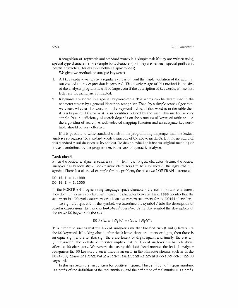
Figure 20.4. The positive integer and real number.

///.-,()*+ L|_ ///.-,()*+ÂÁÀ¿»¼½¾ L|D|_ee

Figure 20.5. The identi�er.

///.-,()*+ _ ///.-,()*+ _ ///.-,()*+ eol //

Not(eol)

EE/.-,()*+ÂÁÀ¿»¼½¾

Figure 20.6. A comment.

the not-visible characters are denoted by their short names, and let ε be the name of the empty cha-racter stream. Not(a) denotes a character distinct from a. The regular expressions are:1. real number: (+ | − | ε)D+.D+(e(+ | − | ε)D+ | ε),2. positive integer and real number: (D+(ε | .)) | (D∗.D+),3. identi�er: (L | _ )(L | D | _ )∗,4. comment: - -(Not(eol))∗eol,5. comment terminated by ## : ##((# | ε)Not(#))∗##,6. string of characters: �(Not(�) | � �)∗ �.

Deterministic �nite automata constructed from regular expressions 2 and 3 are in Figures 20.4and 20.5.

The task of lexical analyser is to determine the text of symbols, but not all the charactersof a regular expression belong to the symbol. As is in the 6th example, the �rst and the last" characters do not belong to the symbol. To unravel this problem, a buffer is created forthe scanner. After recognising of a symbol, the characters of these symbols will be in thebuffer. Now the deterministic �nite automaton is supplemented by a T transfer function,where T (a) means that the character a is inserted into the buffer.

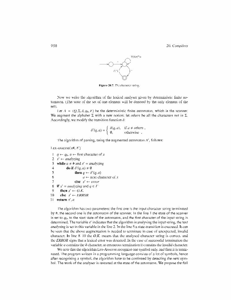
Example 20.2 The 4th and 6th regular expressions of the example 20.1. are supplemented by the Tfunction, automata for these expressions are in Figures 20.6 and 20.7. The automaton of the 4th regularexpression has none T function, since it recognises comments. The automaton of the 6th regularexpression recognises This is a "string" from the character string "This is a ""string""".

958 20. Compilers

///.-,()*+ � ///.-,()*+T (Not(�))

qq

�||/.-,()*+ÂÁÀ¿»¼½¾

T (�)

<<

Figure 20.7. The character string.

Now we write the algorithm of the lexical analyser given by deterministic �nite au-tomaton. (The state of the set of one element will be denoted by the only element of theset).

Let A = (Q,Σ, δ, q0, F) be the deterministic �nite automaton, which is the scanner.We augment the alphabet Σ with a new notion: let others be all the characters not in Σ.Accordingly, we modify the transition function δ:

δ′(q, a) =

{δ(q, a), if a , others ,∅, otherwise .

The algorithm of parsing, using the augmented automaton A′, follows:

L-(x#, A′)1 q← q0, a← �rst character of x2 s′ ← analyzing3 while a , # and s′ = analyzing4 do if δ′(q, a) , ∅5 then q← δ′(q, a)6 a← next character of x7 else s′ ← error8 if s′ = analyzing and q ∈ F9 then s′ ← O.K.

10 else s′ ← ERROR11 return s′, a

The algorithm has two parameters: the �rst one is the input character string terminatedby #, the second one is the automaton of the scanner. In the line 1 the state of the scanneris set to q0, to the start state of the automaton, and the �rst character of the input string isdetermined. The variable s′ indicates that the algorithm is analysing the input string, the textanalysing is set in this variable in the line 2. In the line 5 a state-transition is executed. It canbe seen that the above augmentation is needed to terminate in case of unexpected, invalidcharacter. In line 8�10 the O.K. means that the analysed character string is correct, andthe ERROR signs that a lexical error was detected. In the case of successful termination thevariable a contains the # character, at erroneous termination it contains the invalid character.

We note that the algorithm L-A recognise one symbol only, and then it is termi-nated. The program written in a programming language consists of a lot of symbols, henceafter recognising a symbol, the algorithm have to be continued by detecting the next sym-bol. The work of the analyser is restarted at the state of the automaton. We propose the full


algorithm of the lexical analyser as an exercise (see Exercise 20-1.).

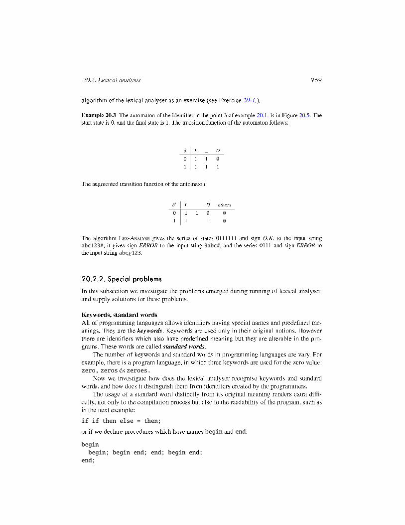
Example 20.3 The automaton of the identi�er in the point 3 of example 20.1. is in Figure 20.5. Thestart state is 0, and the �nal state is 1. The transition function of the automaton follows:

δ L _ D0 1 1 ∅1 1 1 1

The augmented transition function of the automaton:

δ′ L _ D others0 1 1 ∅ ∅1 1 1 1 ∅

The algorithm L-A gives the series of states 0111111 and sign O.K. to the input stringabc123#, it gives sign ERROR to the input sting 9abc#, and the series 0111 and sign ERROR tothe input string abcχ123.

20.2.2. Special problemsIn this subsection we investigate the problems emerged during running of lexical analyser,and supply solutions for these problems.

Keywords, standard wordsAll of programming languages allows identi�ers having special names and prede�ned me-anings. They are the keywords. Keywords are used only in their original notions. Howeverthere are identi�ers which also have prede�ned meaning but they are alterable in the pro-grams. These words are called standard words.

The number of keywords and standard words in programming languages are vary. Forexample, there is a program language, in which three keywords are used for the zero value:zero, zeros és zeroes.

Now we investigate how does the lexical analyser recognise keywords and standardwords, and how does it distinguish them from identi�ers created by the programmers.

The usage of a standard word distinctly from its original meaning renders extra diffi-culty, not only to the compilation process but also to the readability of the program, such asin the next example:if if then else = then;

or if we declare procedures which have names begin and end:

beginbegin; begin end; end; begin end;

end;

960 20. Compilers

Recognition of keywords and standard words is a simple task if they are written usingspecial type characters (for example bold characters), or they are between special pre�x andpost�x characters (for example between apostrophes).

We give two methods to analyse keywords.1. All keywords is written as a regular expression, and the implementation of the automa-

ton created to this expression is prepared. The disadvantage of this method is the sizeof the analyser program. It will be large even if the description of keywords, whose �rstletter are the same, are contracted.

2. Keywords are stored in a special keyword-table. The words can be determined in thecharacter stream by a general identi�er- recogniser. Then, by a simple search algorithm,we check whether this word is in the keyword- table. If this word is in the table thenit is a keyword. Otherwise it is an identi�er de�ned by the user. This method is verysimple, but the efficiency of search depends on the structure of keyword-table and onthe algorithm of search. A well-selected mapping function and an adequate keyword-table should be very effective.If it is possible to write standard words in the programming language, then the lexical

analyser recognises the standard words using one of the above methods. But the meaning ofthis standard word depends of its context. To decide, whether it has its original meaning orit was overde�ned by the programmer, is the task of syntactic analyser.

Look aheadSince the lexical analyser creates a symbol from the longest character stream, the lexicalanalyser has to look ahead one or more characters for the allocation of the right-end of asymbol There is a classical example for this problem, the next two FORTRAN statements:

DO 10 I = 1.1000DO 10 I = 1,1000

In the FORTRAN programming language space-characters are not important characters,they do not play an important part, hence the character between 1 and 1000 decides that thestatement is a DO cycle statement or it is an assignment statement for the DO10I identi�er.

To sign the right end of the symbol, we introduce the symbol / into the description ofregular expressions. Its name is lookahead operator. Using this symbol the description ofthe above DO keyword is the next:

DO / (letter | digit)∗ = (letter | digit)∗,

This de�nition means that the lexical analyser says that the �rst two D and O letters arethe DO keyword, if looking ahead, after the O letter, there are letters or digits, then there isan equal sign, and after this sign there are letters or digits again, and �nally, there is a �, � character. The lookahead operator implies that the lexical analyser has to look aheadafter the DO characters. We remark that using this lookahead method the lexical analyserrecognises the DO keyword even if there is an error in the character stream, such as in theDO2A=3B, character stream, but in a correct assignment statement it does not detect the DOkeyword.

In the next example we concern for positive integers. The de�nition of integer numbersis a pre�x of the de�nition of the real numbers, and the de�nition of real numbers is a pre�x


of the de�nition of real numbers containing explicit power-part.

pozitív egész : D+

pozitív valós : D+.D+

és D+.D+e(+ | − | ε)D+

The automaton for all of these three expressions is the automaton of the longest characterstream, the real number containing explicit power-part.

The problem of the lookahead symbols is resolved using the following algorithm. Putthe character into a buffer, and put an auxiliary information aside this character. This in-formation is �it is invalid�. if the character string, using this red character, is not correct;otherwise we put the type of the symbol into here. If the automaton is in a �nal-state, thenthe automaton recognises a real number with explicit power-part. If the automaton is in aninternal state, and there is no possibility to read a next character, then the longest characterstream which has valid information is the recognised symbol.

Example 20.4 Consider the 12.3e+f# character stream, where the character # is the endsign of theanalysed text. If in this character stream there was a positive integer number in the place of characterf, then this character stream should be a real number. The content of the puffer of lexical analyser:1 integer number12 integer number12. invalid12.3 real number12.3e invalid12.3e+ invalid12.3e+f invalid12.3e+f#

The recognised symbol is the 12.3 real number. The lexical analysing is continued at the text e+f.

The number of lookahead-characters may be determined from the de�nition of the pro-gram language. In the modern languages this number is at most two.

The symbol tableThere are programming languages, for example C, in which small letters and capital lettersare different. In this case the lexical analyser uses characters of all symbols without modi�-cation. Otherwise the lexical analyser converts all characters to their small letter form or allcharacters to capital letter form. It is proposed to execute this transformation in the sourcehandler program.

At the case of simpler programming languages the lexical analyser writes the charactersof the detected symbol into the symbol table, if this symbol is not there. After writingup, or if this symbol has been in the symbol table already, the lexical analyser returns thetable address of this symbol, and writes this information into its output. These data will beimportant at semantic analysis and code generation.

DirectivesIn programming languages the directives serve to control the compiler. The lexical analyseridenti�es directives and recognises their operands, and usually there are further tasks with

962 20. Compilers

these directives.If the directive is the if of the conditional compilation, then the lexical analyser has to

detect all of parameters of this condition, and it has to evaluate the value of the branch. If thisvalue is false, then it has to omit the next lines until the else or endif directive. It meansthat the lexical analyser performs syntactic and semantic checking, and creates code-styleinformation. This task is more complicate if the programming language gives possibility towrite nested conditions.

Other types of directives are the substitution of macros and including �les into thesource text. These tasks are far away from the original task of the lexical analyser.

The usual way to solve these problems is the following. The compiler executes a pre-processing program, and this program performs all of the tasks written by directives.

Exercises20.2-1 Give a regular expression to the comments of a programming language. In this lan-guage the delimiters of comments are /∗ and ∗/, and inside of a comment may occurs / and∗ characters, but ∗/ is forbidden.20.2-2 Modify the result of the previous question if it is supposed that the programminglanguage has possibility to write nested comments.20.2-3 Give a regular expression for positive integer numbers, if the pre- and post-zero cha-racters are prohibited. Give a deterministic �nite automaton for this regular expression.20.2-4 Write a program, which re-creates the original source program from the output oflexical analyser. Pay attention for nice an correct positions of the re-created character stre-ams.

20.3. Syntactic analysisThe perfect de�nition of a programming language includes the de�nition of its syntax andsemantics.

The syntax of the programming languages cannot be written by context free grammars.It is possible by using context dependent grammars, two-level grammars or attribute gram-mars. For these grammars there are not efficient parsing methods, hence the descriptionof a language consists of two parts. The main part of the syntax is given using contextfree grammars, and for the remaining part a context dependent or an attribute grammar isapplied. For example, the description of the program structure or the description of the sta-tement structure belongs to the �rst part, and the type checking, the scope of variables orthe correspondence of formal and actual parameters belong to the second part.

The checking of properties written by context free grammars is called syntactic analysisor parsing. Properties that cannot be written by context free grammars are called form thestatic semantics. These properties are checked by the semantic analyser.

The conventional semantics has the name run-time semantics or dynamic semantics.The dynamic semantics can be given by verbal methods or some interpreter methods, wherethe operation of the program is given by the series of state-alterations of the interpreter andits environment.

We deal with context free grammars, and in this section we will use extended grammarsfor the syntactic analysis. We investigate on methods of checking of properties which are

20.3. Syntactic analysis 963

written by context free grammars. First we give basic notions of the syntactic analysis, thenthe parsing algorithms will be studied.

De�nition 20.1 Let G = (N,T, P, S ) be a grammar. If S∗

=⇒ α and α ∈ (N ∪ T )∗ then αis a sentential form. If S

∗=⇒ x and x ∈ T ∗ then x is a sentence of the language de�ned by

the grammar.The sentence has an important role in parsing. The program written by a programmer

is a series of terminal symbols, and this series is a sentence if it is correct, that is, it has notsyntactic errors.De�nition 20.2 Let G = (N,T, P, S ) be a grammar and α = α1βα2 is a sentential form(α, α1, α2, β ∈ (N ∪ T )∗). We say that β is a phrase of α, if there is a symbol A ∈ N, whichS

∗=⇒ α1Aα2 and A

∗=⇒ β. We say that α is a simple phrase of β, if A→ β ∈ P.

We note that every sentence is phrase. The leftmost simple phrase has an important rolein parsing; it has its own name.De�nition 20.3 The leftmost simple phase of a sentence is the handle.

The leaves of the syntax tree of a sentence are terminal symbols, other points of the treeare nonterminal symbols, and the root symbol of the tree is the start symbol of the grammar.

In an ambiguous grammar there is at least one sentence, which has several syntax trees.It means that this sentence has more than one analysis, and therefore there are several targetprograms for this sentence. This ambiguity raises a lot of problems, therefore the compilerstranslate languages generated by unambiguous grammars only.

We suppose that the grammar G has properties as follows:1. the grammar is cycle free, that is, it has not series of derivations rules A

+=⇒ A (A ∈ N),

2. the grammar is reduced, that is, there are not �unused symbols� in the grammar, all ofnonterminals happen in a derivation, and from all nonterminals we can derive a part ofa sentence. This last property means that for all A ∈ N it is true that S

∗=⇒ αAβ

∗=⇒

αyβ∗

=⇒ xyz, where A∗

=⇒ y and |y| > 0 (α, β ∈ (N ∪ T )∗, x, y, z ∈ T ∗).As it has shown, the lexical analyser translates the program written by a programmer

into series of terminal symbols, and this series is the input of syntactic analyser. The taskof syntactic analyser is to decide if this series is a sentence of the grammar or it is not. Toachieve this goal, the parser creates the syntax tree of the series of symbols. From the knownstart symbol and the leaves of the syntax tree the parser creates all vertices and edges of thetree, that is, it creates a derivation of the program.

If this is possible, then we say that the program is an element of the language. It meansthat the program is syntactically correct.

Hence forward we will deal with left to right parsing methods. These methods read thesymbols of the programs left to right. All of the real compilers use this method.

To create the inner part of the syntax tree there are several methods. One of these met-hods builds the syntax tree from its start symbol S . This method is called top-down method.If the parser goes from the leaves to the symbol S , then it uses the bottom-up parsing met-hod.

We deal with top-down parsing methods in Subsection 20.3.1. We investigate bottom-upparsers in Subsection 20.3.2; now these methods are used in real compilers.

964 20. Compilers

20.3.1. LL(1) parserIf we analyse from top to down then we start with the start symbol. This symbol is the rootof syntax tree; we attempt to construct the syntax tree. Our goal is that the leaves of tree arethe terminal symbols.

First we review the notions that are necessary in the top-down parsing. Then the LL(1)table methods and the recursive descent method will be analysed.

LL(k) grammarsOur methods build the syntax tree top-down and read symbols of the program left to right.For this end we try to create terminals on the left side of sentential forms.

De�nition 20.4 If A → α ∈ P then the leftmost direct derivation of the sentential formxAβ (x ∈ T ∗, α, β ∈ (N ∪ T )∗) is xαβ, and

xAβ =⇒le f tmost

xαβ .

De�nition 20.5 If all of direct derivations in S∗

=⇒ x (x ∈ T ∗) are leftmost, then thisderivation is said to be leftmost derivation, and

S∗

=⇒le f tmost

x .

In a leftmost derivation terminal symbols appear at the left side of the sentential forms.Therefore we use leftmost derivations in all of top-down parsing methods. Hence if we dealwith top-down methods, we do not write the text �leftmost� at the arrows.

One might as well say that we create all possible syntax trees. Reading leaves fromleft to right, we take sentences of the language. Then we compare these sentences with theparseable text and if a sentence is same as the parseable text, then we can read the stepsof parsing from the syntax tree which is belongs to this sentence. But this method is notpractical; generally it is even impossible to apply.

A good idea is the following. We start at the start symbol of the grammar, and usingleftmost derivations we try to create the text of the program. If we use a not suitable deriva-tion at one of steps of parsing, then we �nd that, at the next step, we can not apply a properderivation. At this case such terminal symbols are at the left side of the sentential form, thatare not same as in our parseable text.

For the leftmost terminal symbols we state the theorem as follows.

Theorem 20.6 If S∗

=⇒ xα∗

=⇒ yz (α ∈ (N ∪ T )∗, x, y, z ∈ T ∗) és |x| = |y|, then x = y .

The proof of this theorem is trivial. It is not possible to change the leftmost terminalsymbols x of sentential forms using derivation rules of a context free grammar.

This theorem is used during the building of syntax tree, to check that the leftmost ter-minals of the tree are same as the leftmost symbols of the parseable text. If they are differentthen we created wrong directions with this syntax tree. At this case we have to make a backt-rack, and we have to apply an other derivation rule. If it is impossible (since for examplethere are no more derivation rules) then we have to apply a backtrack once again.

General top-down methods are realized by using backtrack algorithms, but these backt-rack steps make the parser very slow. Therefore we will deal only with grammars such that


S

w A β

w α β

w x

7−→k

Figure 20.8. LL(k) grammar.

have parsing methods without backtracks.The main properties of LL(k) grammars are the following. If, by creating the leftmost

derivation S∗

=⇒ wx (w, x ∈ T ∗), we obtain the sentential form S∗

=⇒ wAβ (A ∈ N, β ∈(N ∪ T )∗) at some step of this derivation, and our goal is to achieve Aβ

∗=⇒ x, then the

next step of the derivation for nonterminal A is determinable unambiguously from the �rstk symbols of x.

To look ahead k symbols we de�ne the function Firstk.

De�nition 20.7 Let Firstk(α) (k ≥ 0, α ∈ (N ∪ T )∗) be the set as follows.

Firstk(α) = {x | α ∗=⇒ xβ and |x| = k} ∪ {x | α ∗

=⇒ x and |x| < k} (x ∈ T ∗, β ∈ (N∪T )∗) .

The set Firstk(x) consists of the �rst k symbols of x; for |x| < k, it consists the full x. Ifα

∗=⇒ ε, then ε ∈ Firstk(α).

De�nition 20.8 The grammar G is a LL(k) grammar (k ≥ 0), if for derivations

S∗

=⇒ wAβ =⇒ wα1β∗

=⇒ wx ,S

∗=⇒ wAβ =⇒ wα2β

∗=⇒ wy

(A ∈ N, x, y,w ∈ T ∗, α1, α2, β ∈ (N ∪ T )∗) the equality

Firstk(x) = Firstk(y)

impliesα1 = α2 .

Using this de�nition, if a grammar is a LL(k) grammar then the k symbol after the parsedx determine the next derivation rule unambiguously (Figure 20.8).

One can see from this de�nition that if a grammar is an LL(k0) grammar then for allk > k0 it is also an LL(k) grammar. If we speak about LL(k) grammar then we also meanthat k is the least number such that the properties of the de�nition are true.

Example 20.5 The next grammar is a LL(1) grammar. Let G = ({A, S }, {a, b}, P, S ) be a grammarwhose derivation rules are:

966 20. Compilers

S → AS | εA→ aA | b

We have to use the derivation S → AS for the start symbol S if the next symbol of the parseable textis a or b. We use the derivation S → ε if the next symbol is the mark #.

Example 20.6 The next grammar is a LL(2) grammar. Let G = ({A, S }, {a, b}, P, S ) be a grammarwhose the derivation rules are:

S → abA | εA→ S aa | b

One can see that at the last step of derivations

S =⇒ abA =⇒ abS aaS→abA=⇒ ababAaa

andS =⇒ abA =⇒ abS aa

S→ε=⇒ abaa

if we look ahead one symbol, then in both derivations we obtain the symbol a. The proper rule forsymbol S is determined to look ahead two symbols (ab or aa).

There are context free grammars such that are not LL(k) grammars. For example thenext grammar is not LL(k) grammar for any k.

Example 20.7 Let G = ({A, B, S }, {a, b, c}, P, S ) be a grammar whose the derivation rules are:S → A | BA→ aAb | abB→ aBc | ac

L(G) consists of sentences aibi és aici (i ≥ 1). If we analyse the sentence ak+1bk+1, then at the �rststep we can not decide by looking ahead k symbols whether we have to use the derivation S → A orS → B, since for all k Firstk(akbk) = Firstk(akck) = ak.

By the de�nition of the LL(k) grammar, if we get the sentential form wAβ using leftmostderivations, then the next k symbol determines the next rule for symbol A. This is stated inthe next theorem.

Theorem 20.9 Grammar G is a LL(k) grammar iff

S∗

=⇒ wAβ, és A→ γ | δ (γ , δ, w ∈ T ∗, A ∈ N, β, γ, δ ∈ (N ∪ T )∗)

impliesFirstk(γβ) ∩ Firstk(δβ) = ∅ .

If there is a A→ ε rule in the grammar, then the set Firstk consists the k length pre�xesof terminal series generated from β. It implies that, for deciding the property LL(k), we haveto check not only the derivation rules, but also the in�nite derivations.

We can give good methods, that are used in the practice, for LL(1) grammars only. Wede�ne the follower-series, which follow a symbol or series of symbols.

De�nition 20.10 Followk(β) = {x | S ∗=⇒ αβγ and x ∈ Firstk(γ)}, and if ε ∈ Followk(β),

then Followk(β) = Followk(β) \ {ε} ∪ {#} (α, β, γ ∈ (N ∪ T )∗, x ∈ T ∗) .


The second part of the de�nition is necessary because if there are no symbols after theβ in the derivation αβγ, that is γ = ε, then the next symbol after β is the mark # only.

Follow1(A) (A ∈ N) consists of terminal symbols that can be immediately after thesymbol A in the derivation

S∗

=⇒ αAγ∗

=⇒ αAw (α, γ ∈ (N ∪ T )∗, w ∈ T ∗).

Theorem 20.11 The grammar G is a LL(1) grammar iff, for all nonterminal A and for allderivation rules A→ γ | δ,

First1(γFollow1(A)) ∩ First1(δFollow1(A)) = ∅ .In this theorem the expression First1(γFollow1(A)) means that we have to concatenate

to γ the elements of set Follow1(A) separately, and for all elements of this new set we haveto apply the function First1.

It is evident that theorem 20.11 is suitable to decide whether a grammar is LL(1) or it isnot.

Hence forward we deal with LL(1) languages determined by LL(1) grammars, and weinvestigate the parsing methods of LL(1) languages. For the sake of simplicity, we omitindexes from the names of functions First1 és Follow1.

The elements of the set First(α) are determined using the next algorithm.

F(α)1 if α = ε2 then F ← {ε}3 if α = a, where a ∈ T4 then F ← {a}5 if α = A, where A ∈ N6 then if A→ ε ∈ P7 then F ← {ε}8 else F ← ∅9 for all A→ Y1Y2 . . . Ym ∈ P (m ≥ 1)

10 do F ← F ∪ (F(Y1) \ {ε})11 for k ← 1 to m − 112 do if Y1Y2 . . . Yk

∗=⇒ ε

13 then F ← F ∪ (F(Yk+1) \ {ε})14 if Y1Y2 . . . Ym

∗=⇒ ε

15 then F ← F ∪ {ε}16 if α = Y1Y2 . . . Ym (m ≥ 2)17 then F ← (F(Y1) \ {ε})18 for k ← 1 to m − 119 do if Y1Y2 . . . Yk

∗=⇒ ε

20 then F ← F ∪ (F(Yk+1) \ {ε})21 if Y1Y2 . . . Ym

∗=⇒ ε

22 then F ← F ∪ {ε}23 return F

968 20. Compilers

S

x B α

x a y

S

x b α

x a y

Figure 20.9. The sentential form and the analysed text.

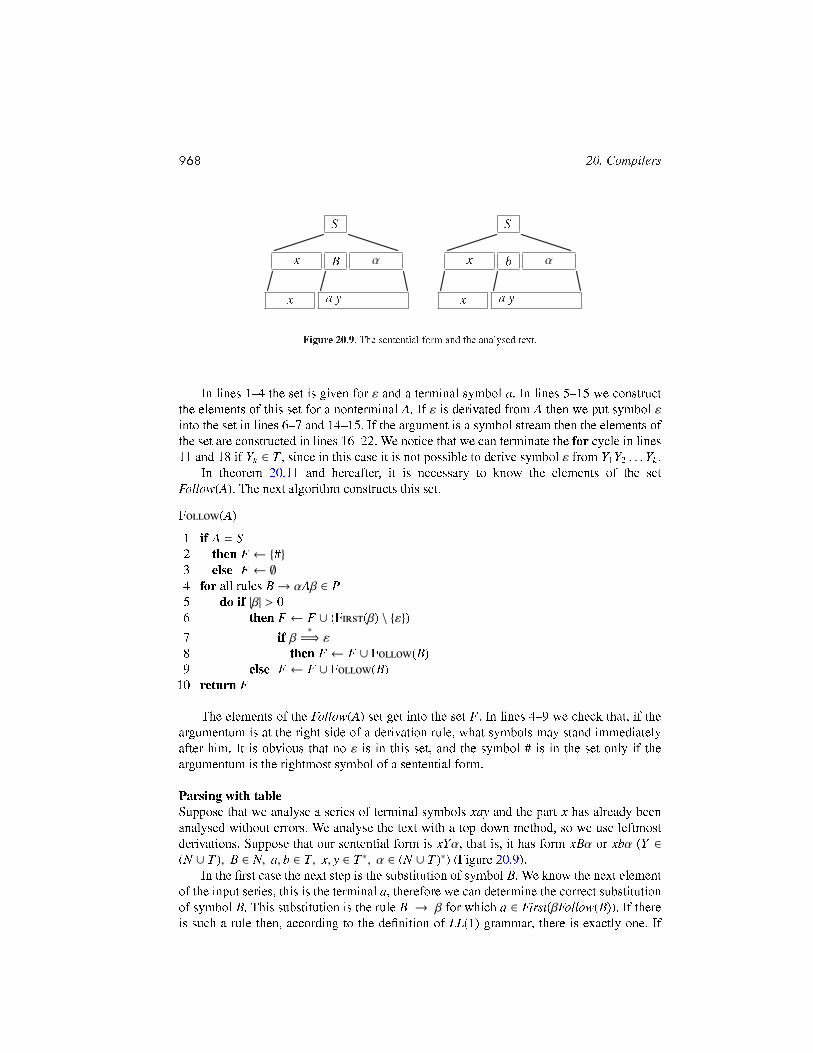
In lines 1�4 the set is given for ε and a terminal symbol a. In lines 5�15 we constructthe elements of this set for a nonterminal A. If ε is derivated from A then we put symbol εinto the set in lines 6�7 and 14�15. If the argument is a symbol stream then the elements ofthe set are constructed in lines 16�22. We notice that we can terminate the for cycle in lines11 and 18 if Yk ∈ T , since in this case it is not possible to derive symbol ε from Y1Y2 . . . Yk.

In theorem 20.11 and hereafter, it is necessary to know the elements of the setFollow(A). The next algorithm constructs this set.

F(A)1 if A = S2 then F ← {#}3 else F ← ∅4 for all rules B→ αAβ ∈ P5 do if |β| > 06 then F ← F ∪ (F(β) \ {ε})7 if β ∗

=⇒ ε8 then F ← F ∪ F(B)9 else F ← F ∪ F(B)

10 return F

The elements of the Follow(A) set get into the set F. In lines 4�9 we check that, if theargumentum is at the right side of a derivation rule, what symbols may stand immediatelyafter him. It is obvious that no ε is in this set, and the symbol # is in the set only if theargumentum is the rightmost symbol of a sentential form.

Parsing with tableSuppose that we analyse a series of terminal symbols xay and the part x has already beenanalysed without errors. We analyse the text with a top-down method, so we use leftmostderivations. Suppose that our sentential form is xYα, that is, it has form xBα or xbα (Y ∈(N ∪ T ), B ∈ N, a, b ∈ T, x, y ∈ T ∗, α ∈ (N ∪ T )∗) (Figure 20.9).

In the �rst case the next step is the substitution of symbol B. We know the next elementof the input series, this is the terminal a, therefore we can determine the correct substitutionof symbol B. This substitution is the rule B → β for which a ∈ First(βFollow(B)). If thereis such a rule then, according to the de�nition of LL(1) grammar, there is exactly one. If


x a y #

parser

v

X

α

#

¾

6

?

Figure 20.10. The structure of the LL(1) parser.

there is not such a rule, then a syntactic error was found.In the second case the next symbol of the sentential form is the terminal symbol b, thus

we look out for the symbol b as the next symbol of the analysed text. If this comes true, thatis, a = b, then the symbol a is a correct symbol and we can go further. We put the symbola into the already analysed text. If a , b, then here is a syntactic error. We can see that theposition of the error is known, and the erroneous symbol is the terminal symbol a.

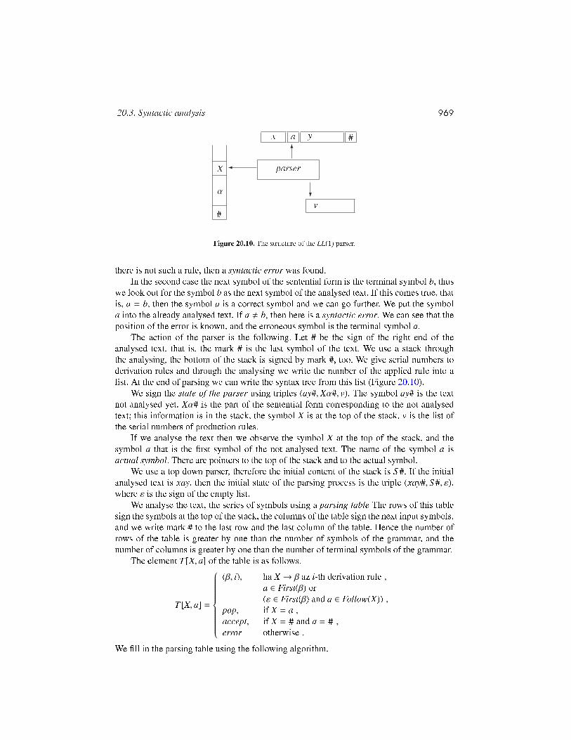
The action of the parser is the following. Let # be the sign of the right end of theanalysed text, that is, the mark # is the last symbol of the text. We use a stack throughthe analysing, the bottom of the stack is signed by mark #, too. We give serial numbers toderivation rules and through the analysing we write the number of the applied rule into alist. At the end of parsing we can write the syntax tree from this list (Figure 20.10).

We sign the state of the parser using triples (ay#, Xα#, v). The symbol ay# is the textnot analysed yet. Xα# is the part of the sentential form corresponding to the not analysedtext; this information is in the stack, the symbol X is at the top of the stack. v is the list ofthe serial numbers of production rules.

If we analyse the text then we observe the symbol X at the top of the stack, and thesymbol a that is the �rst symbol of the not analysed text. The name of the symbol a isactual symbol. There are pointers to the top of the stack and to the actual symbol.

We use a top down parser, therefore the initial content of the stack is S #. If the initialanalysed text is xay, then the initial state of the parsing process is the triple (xay#, S #, ε),where ε is the sign of the empty list.

We analyse the text, the series of symbols using a parsing table The rows of this tablesign the symbols at the top of the stack, the columns of the table sign the next input symbols,and we write mark # to the last row and the last column of the table. Hence the number ofrows of the table is greater by one than the number of symbols of the grammar, and thenumber of columns is greater by one than the number of terminal symbols of the grammar.

The element T [X, a] of the table is as follows.

T [X, a] =

(β, i), ha X → β az i-th derivation rule ,a ∈ First(β) or(ε ∈ First(β) and a ∈ Follow(X)) ,

pop, if X = a ,accept, if X = # and a = # ,error otherwise .

We �ll in the parsing table using the following algorithm.

970 20. Compilers

LL(1)---(G)1 for all A ∈ N2 do if A→ α ∈ P the i-th rule3 then for all a ∈ F(α)- ra4 do T [A, a]← (α, i)5 if ε ∈ F(α)6 then for all a ∈ F(A)7 do T [A, a]← (α, i)8 for all a ∈ T9 do T [a, a]← pop

10 T [#, #]← accept11 for all X ∈ (N ∪ T ∪ {#}) and all a ∈ (T ∪ {#})12 do if T [X, a] = �empty�13 then T [X, a]← error14 return T

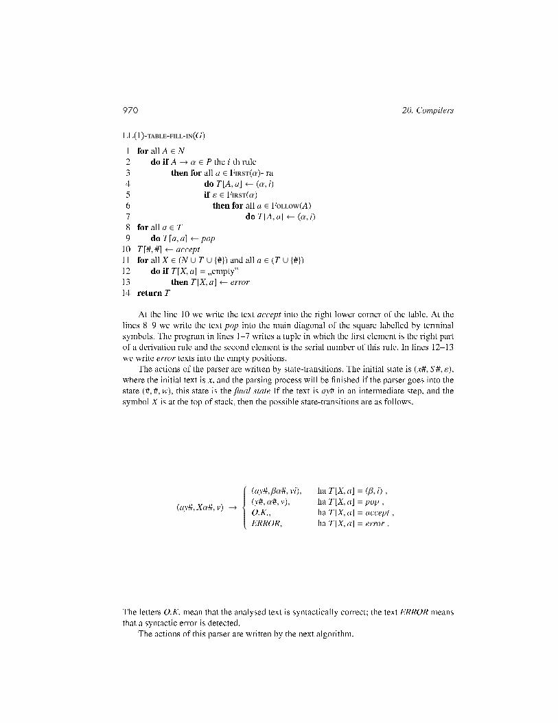
At the line 10 we write the text accept into the right lower corner of the table. At thelines 8�9 we write the text pop into the main diagonal of the square labelled by terminalsymbols. The program in lines 1�7 writes a tuple in which the �rst element is the right partof a derivation rule and the second element is the serial number of this rule. In lines 12�13we write error texts into the empty positions.

The actions of the parser are written by state-transitions. The initial state is (x#, S #, ε),where the initial text is x, and the parsing process will be �nished if the parser goes into thestate (#, #,w), this state is the �nal state If the text is ay# in an intermediate step, and thesymbol X is at the top of stack, then the possible state-transitions are as follows.

(ay#, Xα#, v) →

(ay#, βα#, vi), ha T [X, a] = (β, i) ,(y#, α#, v), ha T [X, a] = pop ,O.K., ha T [X, a] = accept ,ERROR, ha T [X, a] = error .

The letters O.K. mean that the analysed text is syntactically correct; the text ERROR meansthat a syntactic error is detected.

The actions of this parser are written by the next algorithm.


LL(1)-(xay#,T )1 s← (xay#, S #, ε), s′ ← analyze2 repeat3 if s = (ay#, Aα#, v) és T [A, a] = (β, i)4 then s← (ay#, βα#, vi)5 else if s = (ay#, aα#, v)6 then s← (y#, α#, v) B Then T [a, a] = pop.7 else if s = (#, #, v)8 then s′ ← O.K. B Then T [#, #] = accept.9 else s′ ← ERROR B Then T [A, a] = error.

10 until s′ = O.K. or s′ = ERROR11 return s′, s

The input parameters of this algorithm are the text xay and the parsing table T . Thevariable s′ describes the state of the parser: its value is analyse, during the analysis, and it iseither O.K. or ERROR. at the end. The parser determines his action by the actual symbol aand by the symbol at the top of the stack, using the parsing table T . In the line 3�4 the parserbuilds the syntax tree using the derivation rule A → β. In lines 5�6 the parser executes ashift action, since there is a symbol a at the top of the stack. At lines 8�9 the algorithm�nishes his work if the stack is empty and it is at the end of the text, otherwise a syntacticerror was detected. At the end of this work the result is O.K. or ERROR in the variable s′,and, as a result, there is the triple s at the output of this algorithm. If the text was correct,then we can create the syntax tree of the analysed text from the third element of the triple. Ifthere was an error, then the �rst element of the triple points to the position of the erroneoussymbol.

Example 20.8 Let G be a grammar G = ({E, E′,T, T ′, F}, {+, ∗, (, ), i}, P, E), where the set P ofderivation rules:

E → T E′E′ → +T E′ | εT → FT ′T ′ → ∗FT ′ | εF → (E) | i>From these rules we can determine the Follow(A) sets. To �ll in the parsing table, the following

sets are required:First(T E′) = {(, i},First(+T E′) = {+},First(FT ′) = {(, i},First(∗FT ′) = {∗},First((E)) = {(},First(i) = {i},Follow(E′) = {), #},Follow(T ′) = {+, ), #}.The parsing table is as follows. The empty positions in the table mean errors

972 20. Compilers

+ * ( ) i #

E (T E′, 1) (T E′, 1)E′ (+T E′, 2) (ε, 3) (ε, 3)T (FT ′, 4) (FT ′, 4)T ′ (ε, 6) (∗FT ′, 5) (ε, 6) (ε, 6)F ((E), 7) (i, 8)+ pop* pop( pop) popi pop# accept

Example 20.9 Using the parsing table of the previous example, analyse the text i + i ∗ i.

(i + i ∗ i#, S #, ε) (T E′ ,1)−−−−−−→ ( i + i ∗ i#, T E′#, 1 )(FT ′ ,4)−−−−−−→ ( i + i ∗ i#, FT ′E′#, 14 )(i,8)−−−→ ( i + i ∗ i#, iT ′E′#, 148 )pop−−−→ ( +i ∗ i#, T ′E′#, 148 )(ε,6)−−−→ ( +i ∗ i#, E′#, 1486 )(+T E′ ,2)−−−−−−−→ ( +i ∗ i#, +T E′#, 14862 )pop−−−→ ( i ∗ i#, T E′#, 14862 )(FT ′ ,4)−−−−−−→ ( i ∗ i#, FT ′E′#, 148624 )(i,8)−−−→ ( i ∗ i#, iT ′E′#, 1486248 )pop−−−→ ( ∗i#, T ′E′#, 1486248 )(∗FT ′ ,5)−−−−−−→ ( ∗i#, ∗FT ′E′#, 14862485 )pop−−−→ ( i#, FT ′E′#, 14862485 )(i,8)−−−→ ( i#, iT ′E′#, 148624858 )pop−−−→ ( #, T ′E′#, 148624858 )(ε,6)−−−→ ( #, E′#, 1486248586 )(ε,3)−−−→ ( #, #, 14862485863 )accept−−−−−→ O.K.

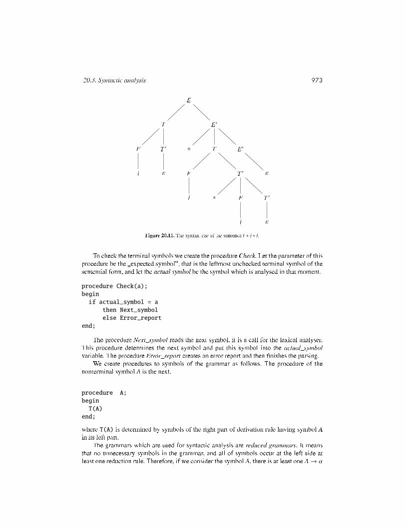
The syntax tree of the analysed text is the Figure 20.11.

Recursive-descent parsing methodThere is another frequently used method for the backtrackless top-down parsing. Its essenceis that we write a real program for the applied grammar. We create procedures to the symbolsof grammar, and using these procedures the recursive procedure calls realize the stack of theparser and the stack management. This is a top-down parsing method, and the procedurescall each other recursively; it is the origin of the name of this method, that is, recursive-descent method


E

~~~~

~~~~

@@@@

@@@@

T

~~~~

~~~~

E′

~~~~

~~~~

AAAA

AAAA

F T ′ + T

~~~~

~~~~

AAAA

AAAA

E′

AAAA

AAAA

i ε F T ′

}}}}

}}}}

AAAA

AAAA

ε

i ∗ F T ′

i ε

Figure 20.11. The syntax tree of the sentence i + i ∗ i.

To check the terminal symbols we create the procedure Check. Let the parameter of thisprocedure be the �expected symbol�, that is the leftmost unchecked terminal symbol of thesentential form, and let the actual symbol be the symbol which is analysed in that moment.

procedure Check(a);begin

if actual_symbol = athen Next_symbolelse Error_report

end;

The procedure Next_symbol reads the next symbol, it is a call for the lexical analyser.This procedure determines the next symbol and put this symbol into the actual_symbolvariable. The procedure Error_report creates an error report and then �nishes the parsing.

We create procedures to symbols of the grammar as follows. The procedure of thenonterminal symbol A is the next.

procedure A;begin

T(A)end;

where T(A) is determined by symbols of the right part of derivation rule having symbol Ain its left part.

The grammars which are used for syntactic analysis are reduced grammars. It meansthat no unnecessary symbols in the grammar, and all of symbols occur at the left side atleast one reduction rule. Therefore, if we consider the symbol A, there is at least one A→ α

974 20. Compilers

production rule.1. If there is only one production rule for the symbol A,

(a) let the program of the rule A→ a is as follows: Check(a),(b) for the rule A→ B we give the procedure call B ,(c) for the rule A→ X1X2 . . . Xn (n ≥ 2) we give the next block:

beginT(X_1);T(X_2);...T(X_n)

end;

2. If there are more rules for the symbol A:

(a) If the rules A → α1 | α2 | . . . | αn are ε-free, that is from αi (1 ≤ i ≤ n) it is notpossible to deduce ε, then T(A)

case actual_symbol ofFirst(alpha_1) : T(alpha_1);First(alpha_2) : T(alpha_2);...First(alpha_n) : T(alpha_n)

end;

where First(alpha_i) is the sign of the set First(αi).We note that this is the �rst point of the method of recursive-descent parser wherewe use the fact that the grammar is an LL(1) grammar.

(b) We use the LL(1) grammar to write a programming language, therefore it is notcomfortable to require that the grammar is a ε-free grammar. For the rules A →α1 | α2 | . . . | αn−1 | ε we create the next T(A) program:case actual_symbol of

First(alpha_1) : T(alpha_1);First(alpha_2) : T(alpha_2);...First(alpha_(n-1)) : T(alpha_(n-1));Follow(A) : skip

end;

where Follow(A) is the set Follow(A).In particular, if the rules A→ α1 | α2 | . . . | αn for some i (1 ≤ i ≤ n) αi

∗=⇒ ε, that

is ε ∈ First(αi), then the i-th row of the case statement isFollow(A) : skip

In the program T(A), if it is possible, we use if-then-else or while statement ins-tead of the statement case.

The start procedure, that is the main program of this parsing program, is the procedurewhich is created for the start symbol of the grammar.


We can create the recursive-descent parsing program with the next algorithm. The inputof this algorithm is the grammar G, and the result is parsing program P. In this algorithm weuse a W- procedure, which concatenates the new program lines to the programP. We will not go into the details of this algorithm.

C--(G)1 P← ∅2 W-(3 procedure Check(a);4 begin5 if actual_symbol = a6 then Next_symbol7 else Error_report8 end;9 )

10 for all symbol A ∈ N of the grammar G11 do if A = S12 then W-(13 program S;14 begin15 R--(S , P)16 end.17 )18 else W-(19 procedure A;20 begin21 R--(A, P)22 end;23 )24 return P

The algorithm creates the Check procedure in lines 2�9/ Then, for all nonterminals ofgrammar G, it determines their procedures using the algorithm R--. In the lines11�17, we can see that for the start symbol S we create the main program. The output ofthe algorithm is the parsing program.

R--(A, P)1 if there is only one rule A→ α2 then R--1(α, P) B A→ α.3 else R--2(A, (α1, . . . , αn), P) B A→ α1 | · · · | αn.4 return P

The form of the statements of the parsing program depends on the derivation rules ofthe symbol A. Therefore the algorithm R- - divides the next tasks into two parts.The algorithm R--1 deals with the case when there is only one derivation rule,and the algorithm R--2 creates the program for the alternatives.

976 20. Compilers

R--1(α, P)1 if α = a2 then W-(3 Check(a)4 )5 if α = B6 then W-(7 B8 )9 if α = X1X2 . . . Xn (n ≥ 2)

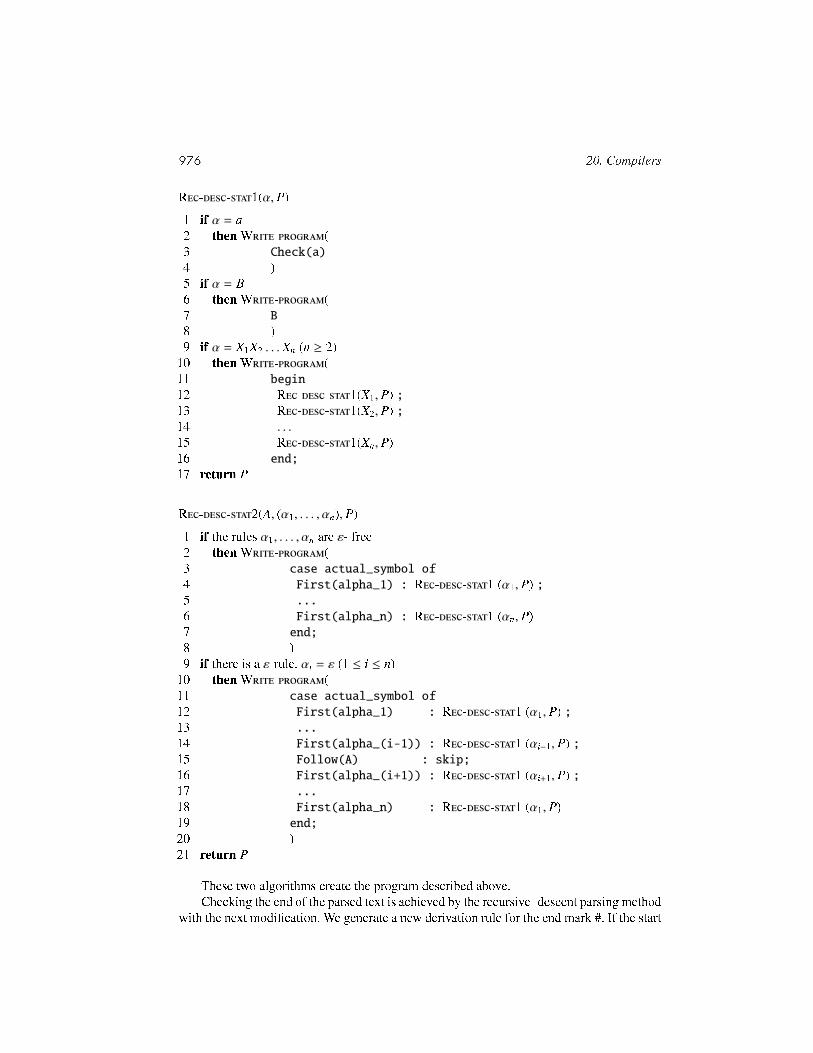
10 then W-(11 begin12 R--1(X1, P) ;13 R--1(X2, P) ;14 . . .15 R--1(Xn, P)16 end;17 return P

R--2(A, (α1, . . . , αn), P)1 if the rules α1, . . . , αn are ε- free2 then W-(3 case actual_symbol of4 First(alpha_1) : R--1 (α1, P) ;5 ...6 First(alpha_n) : R--1 (αn, P)7 end;8 )9 if there is a ε-rule, αi = ε (1 ≤ i ≤ n)

10 then W-(11 case actual_symbol of12 First(alpha_1) : R--1 (α1, P) ;13 ...14 First(alpha_(i-1)) : R--1 (αi−1, P) ;15 Follow(A) : skip;16 First(alpha_(i+1)) : R--1 (αi+1, P) ;17 ...18 First(alpha_n) : R--1 (α1, P)19 end;20 )21 return P

These two algorithms create the program described above.Checking the end of the parsed text is achieved by the recursive- descent parsing method

with the next modi�cation. We generate a new derivation rule for the end mark #. If the start


symbol of the grammar is S , then we create the new rule S ′ → S #, where the new symbolS ′ is the start symbol of our new grammar. The mark # is considered as terminal symbol.Then we generate the parsing program for this new grammar.

Example 20.10 We augment the grammar of the Example 20.8. in the above manner. The productionrules are as follows.

S ′ → E#E → T E′E′ → +T E′ | εT → FT ′T ′ → ∗FT ′ | εF → (E) | iIn the example 20.8. we give the necessary First and Follow sets. We use the next sets:First(+T E′) = {+},First(∗FT ′) = {∗},First((E)) = {(},First(i) = {i},Follow(E′) = {), #},Follow(T ′) = {+, ), #}.In the comments of the program lines we give the using of these sets. The �rst characters of the

comment are the character pair --.The program of the recursive-descent parser is the following.

program S’;begin

E;Check(#)

end.procedure E;begin

T;E’

end;procedure E’;begin

case actual_symbol of+ : begin -- First(+TE’)

Check(+);T;E’

end;),# : skip -- Follow(E’)end

end;procedure T;begin

F;T’

end;procedure T’;

978 20. Compilers

begincase actual_symbol of* : begin -- First(*FT’)

Check(*);F;T’

end;+,),# : skip -- Follow(T’)end

end;procedure F;begin

case actual_symbol of( : begin -- First((E))

Check(();E;Check())

end;i : Check(i) -- First(i)end

end;

We can see that the main program of this parser belongs to the symbol S ′.

20.3.2. LR(1) parsingIf we analyse from bottom to up, then we start with the program text. We search the handleof the sentential form, and we substitute the nonterminal symbol that belongs to the handle,for this handle. After this �rst step, we repeat this procedure several times. Our goal is toachieve the start symbol of the grammar. This symbol will be the root of the syntax tree, andby this time the terminal symbols of the program text are the leaves of the tree.

First we review the notions which are necessary in the parsing.To analyse bottom-up, we have to determine the handle of the sentential form. The

problem is to create a good method which �nds the handle, and to �nd the best substitutionif there are more than one possibilities.

De�nition 20.12 If A → α ∈ P, then the rightmost substitution of the sentential formβAx (x ∈ T ∗, α, β ∈ (N ∪ T )∗) is βαx, that is

βAx =⇒rightmost

βαx .

De�nition 20.13 If the derivation S∗

=⇒ x (x ∈ T ∗) all of the substitutions were rightmostsubstitution, then this derivation is a rightmost derivation,

S∗

=⇒rightmost

x .

In a rightmost derivation, terminal symbols are at the right side of the sentential form.


By the connection of the notion of the handle and the rightmost derivation, if we apply thesteps of a rightmost derivation backwards, then we obtain the steps of a bottom-up parsing.Hence the bottom-up parsing is equivalent with the �inverse� of a rightmost derivation.Therefore, if we deal with bottom-up methods, we will not write the text "rightmost" at thearrows.

General bottom-up parsing methods are realized by using backtrack algorithms. Theyare similar to the top-down parsing methods. But the backtrack steps make the parser veryslow. Therefore we only deal with grammars such that have parsing methods without backt-racks.

Hence forward we produce a very efficient algorithm for a large class of context-freegrammars. This class contains the grammars for the programming languages.

The parsing is called LR(k) parsing; the grammar is called LR(k) grammar. LR meansthe "Left to Right" method, and k means that if we look ahead k symbols then we candetermine the handles of the sentential forms. The LR(k) parsing method is a shift-reducemethod.

We deal with LR(1) parsing only, since for all LR(k) (k > 1) grammar there is an equi-valent LR(1) grammar. This fact is very important for us since, using this type of grammars,it is enough to look ahead one symbol in all cases.

Creating LR(k) parsers is not an easy task. However, there are such standard programs(for example the yacc in UNIX systems), that create the complete parsing program fromthe derivation rules of a grammar. Using these programs the task of writing parsers is nottoo hard.

After studying the LR(k) grammars we will deal with the LALR(1) parsing method. Thismethod is used in the compilers of modern programming languages.

LR(k) grammarsAs we did previously, we write a mark # to the right end of the text to be analysed. Weintroduce a new nonterminal symbol S ′ and a new rule S ′ → S into the grammar.

De�nition 20.14 Let G′ be the augmented grammar belongs to grammar G =

(N,T, P, S ), where G′ augmented grammar

G′ = (N ∪ {S ′},T, P ∪ {S ′ → S }, S ′) .Assign serial numbers to the derivation rules of grammar, and let S ′ → S be the 0th

rule. Using this numbering, if we apply the 0th rule, it means that the parsing process isconcluded and the text is correct.

We notice that if the original start symbol S does not happen on the right side of anyrules, then there is no need for this augmentation. However, for the sake of generality, wedeal with augmented grammars only.

De�nition 20.15 The augmented grammar G′ is an LR(k) grammar (k ≥ 0), if for deri-vations

S ′∗

=⇒ αAw =⇒ αβw ,

S ′∗

=⇒ γBx =⇒ γδx = αβy(A, B ∈ N, x, y,w ∈ T ∗, α, β, γ, δ ∈ (N ∪ T )∗) the equality

Firstk(w) = Firstk(y)

980 20. Compilers

S ′

α A w

α β w

7−→k

S ′

γ B x

γ δ x

α β y

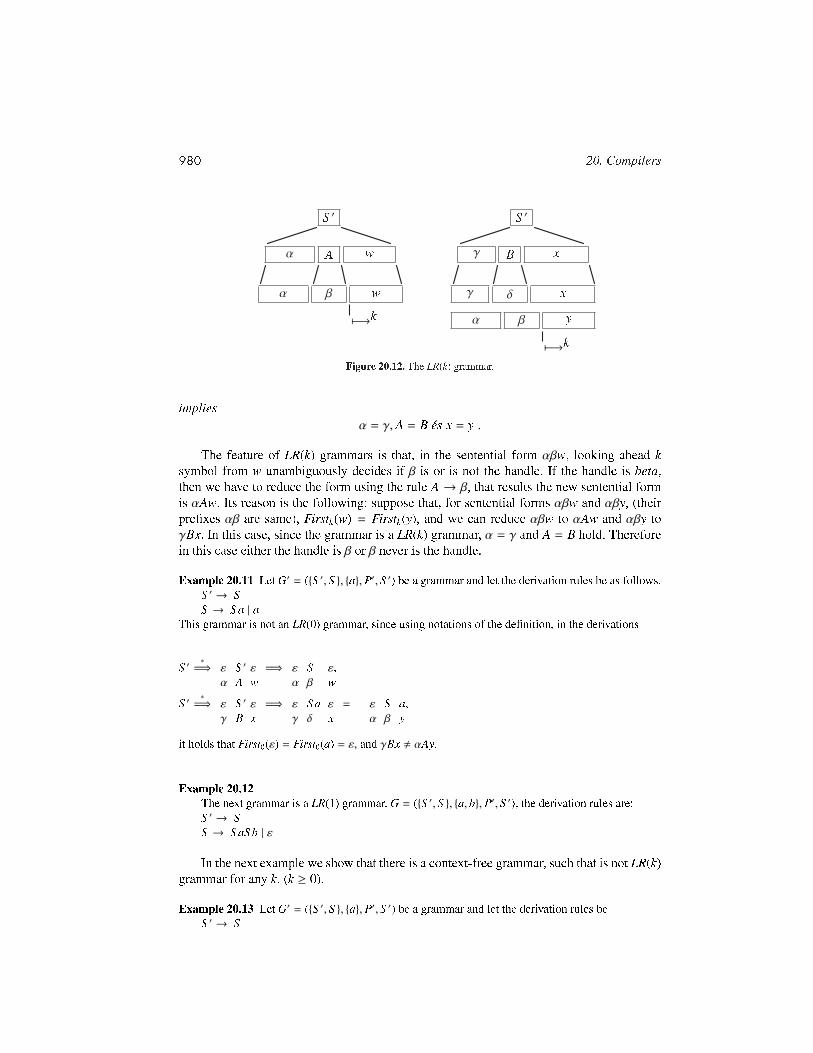
7−→kFigure 20.12. The LR(k) grammar.

impliesα = γ, A = B és x = y .

The feature of LR(k) grammars is that, in the sentential form αβw, looking ahead ksymbol from w unambiguously decides if β is or is not the handle. If the handle is beta,then we have to reduce the form using the rule A → β, that results the new sentential formis αAw. Its reason is the following: suppose that, for sentential forms αβw and αβy, (theirpre�xes αβ are same), Firstk(w) = Firstk(y), and we can reduce αβw to αAw and αβy toγBx. In this case, since the grammar is a LR(k) grammar, α = γ and A = B hold. Thereforein this case either the handle is β or β never is the handle.

Example 20.11 Let G′ = ({S ′, S }, {a}, P′, S ′) be a grammar and let the derivation rules be as follows.S ′ → SS → S a | a

This grammar is not an LR(0) grammar, since using notations of the de�nition, in the derivations

S ′∗

=⇒ ε S ′ ε =⇒ ε S ε,α A w α β w

S ′∗

=⇒ ε S ′ ε =⇒ ε S a ε = ε S a,γ B x γ δ x α β y

it holds that First0(ε) = First0(a) = ε, and γBx , αAy.

Example 20.12The next grammar is a LR(1) grammar. G = ({S ′, S }, {a, b}, P′, S ′), the derivation rules are:S ′ → SS → S aS b | ε

In the next example we show that there is a context-free grammar, such that is not LR(k)grammar for any k. (k ≥ 0).

Example 20.13 Let G′ = ({S ′, S }, {a}, P′, S ′) be a grammar and let the derivation rules beS ′ → S


S → aS a | aNow for all k (k ≥ 0)

S ′∗

=⇒ akS ak =⇒ akaak = a2k+1 ,

S ′∗

=⇒ ak+1S ak+1 =⇒ ak+1aak+1 = a2k+3 ,

andFirstk(ak) = Firstk(aak+1) = ak ,

butak+1S ak+1 , akS ak+2 .

It is not sure that, for a LL(k) (k > 1) grammar, we can �nd an equivalent LL(1) gram-mar. However, LR(k) grammars have this nice property.

Theorem 20.16 For all LR(k) (k > 1) grammar there is an equivalent LR(1) grammar.

The great signi�cance of this theorem is that it makes sufficient to study the LR(1)grammars instead of LR(k) (k > 1) grammars.

LR(1) canonical setsNow we de�ne a very important notion of the LR parsings.

De�nition 20.17 If β is the handle of the αβx (α, β ∈ (N ∪ T )∗, x ∈ T ∗) sentential form,then the pre�xes of αβ are the viable pre�xes of αβx.

Example 20.14 Let G′ = ({E,T, S ′}, {i,+, (, )}, P′, S ′) be a grammar and the derivation rule as follows.(0) S ′ → E(1) E → T(2) E → E + T(3) T → i(4) T → (E)E + (i + i) is a sentential form, and the �rst i is the handle. The viable pre�xes of this sentential

form are E, E+, E + (, E + (i.

By the above de�nition, symbols after the handle are not parts of any viable pre�x.Hence the task of �nding the handle is the task of �nding the longest viable pre�x.

For a given grammar, the set of viable pre�xes is determined, but it is obvious that thesize of this set is not always �nite.

The signi�cance of viable pre�xes are the following. We can assign states of a determi-nistic �nite automaton to viable pre�xes, and we can assign state transitions to the symbolsof the grammar. From the initial state we go to a state along the symbols of a viable pre�x.Using this property, we will give a method to create an automaton that executes the task ofparsing.

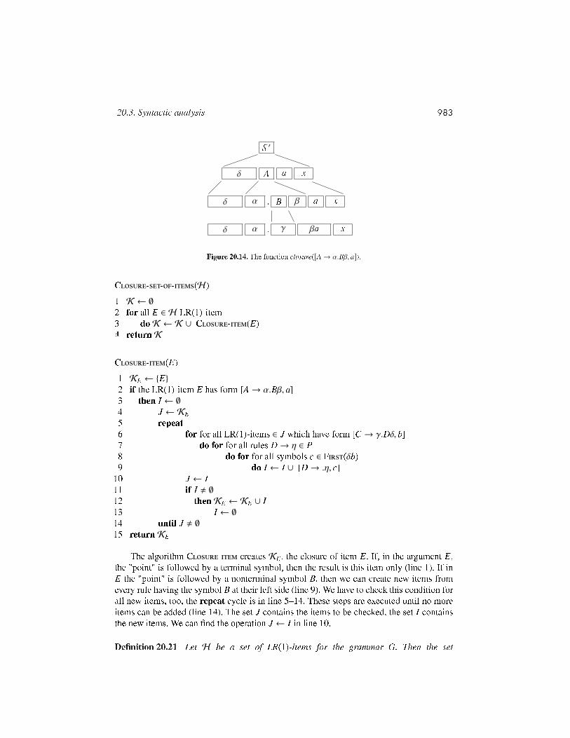
De�nition 20.18 If A→ αβ is a rule of a G′ grammar, then let[A→ α.β, a] , (a ∈ T ∪ {#}) ,

be a LR(1)-item, where A → α.β is the core of the LR(1)-item, and a is the lookaheadsymbol of the LR(1)-item.

982 20. Compilers

A

α . β a

Figure 20.13. The [A→ α.β, a] LR(1) -item.

The lookahead symbol is instrumental in reduction, i.e. it has form [A→ α., a]. It meansthat we can execute reduction only if the symbol a follows the handle alpha.

De�nition 20.19 The LR(1)-item [A→ α.β, a] is valid for the viable pre�x γα if

S ′∗

=⇒ γAx =⇒ γαβx (γ ∈ (N ∪ T )∗, x ∈ T ∗) ,

and a is the �rst symbol of x or if x = ε then a = #.

Example 20.15 Let G′ = ({S ′, S , A}, {a, b}, P′, S ′) a grammar and the derivation rules as follows.(0) S ′ → S(1) S → AA(2) A→ aA(3) A→ bUsing these rules, we can derive S ′

∗=⇒ aaAab =⇒ aaaAab. Here aaa is a viable pre�x,

and [A→ a.A, a] is valid for this viable pre�x. Similarly, S ′∗

=⇒ AaA =⇒ AaaA, and LR(1)-item[A→ a.A, #] is valid for viable pre�x Aaa.

Creating a LR(1) parser, we construct the canonical sets of LR(1)-items. To achieve thiswe have to de�ne the closure and read functions.

De�nition 20.20 Let the set H be a set of LR(1)-items for a given grammar. The setclosure(H) consists of the next LR(1)-items:

1. every element of the setH is an element of the set closure(H),

2. if [A→ α.Bβ, a] ∈ closure(H), and B → γ is a derivation rule of the grammar, then[B→ .γ, b] ∈ closure(H) for all b ∈ First(βa),

3. the set closure(H) is needed to expand using the step 2 until no more items can beadded to it.

By de�nitions, if the LR(1)-item [A→ α.Bβ, a] is valid for the viable pre�x δα, thenthe LR(1)-item [B→ .γ, b] is valid for the same viable pre�x in the case of b ∈ First(βa).(Figure 20.14). It is obvious that the function closure creates all of LR(1)-items which arevalid for viable pre�x δα.

We can de�ne the function closure(H), i.e. the closure of setH by the following algo-rithm. The result of this algorithm is the set K .


S ′

δ A a x

δ α . B β a x

δ α . γ βa x

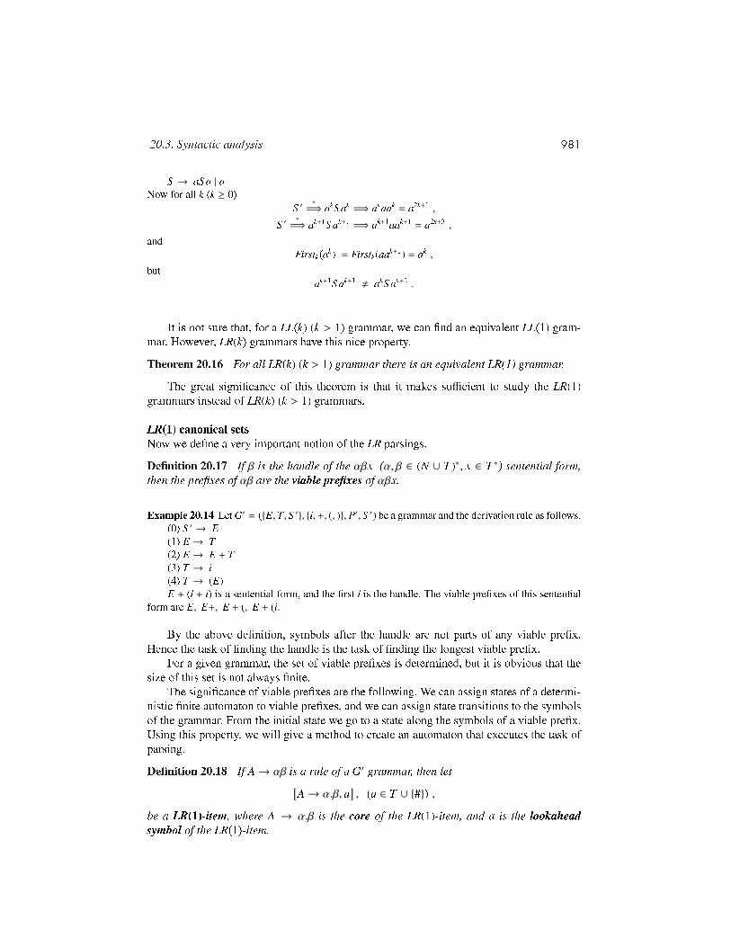
Figure 20.14. The function closure([A→ α.Bβ, a]).

C---(H)1 K ← ∅2 for all E ∈ H LR(1)-item3 do K ← K ∪ C-(E)4 return K

C-(E)1 KE ← {E}2 if the LR(1)-item E has form [A→ α.Bβ, a]3 then I ← ∅4 J ← KE5 repeat6 for for all LR(1)-items ∈ J which have form [C → γ.Dδ, b]7 do for for all rules D→ η ∈ P8 do for for all symbols c ∈ F(δb)9 do I ← I ∪ [D→ .η, c]

10 J ← I11 if I , ∅12 then KE ← KE ∪ I13 I ← ∅14 until J , ∅15 return KE

The algorithm C- creates KE , the closure of item E. If, in the argument E,the "point" is followed by a terminal symbol, then the result is this item only (line 1). If inE the "point" is followed by a nonterminal symbol B, then we can create new items fromevery rule having the symbol B at their left side (line 9). We have to check this condition forall new items, too, the repeat cycle is in line 5�14. These steps are executed until no moreitems can be added (line 14). The set J contains the items to be checked, the set I containsthe new items. We can �nd the operation J ← I in line 10.

De�nition 20.21 Let H be a set of LR(1)-items for the grammar G. Then the set

984 20. Compilers

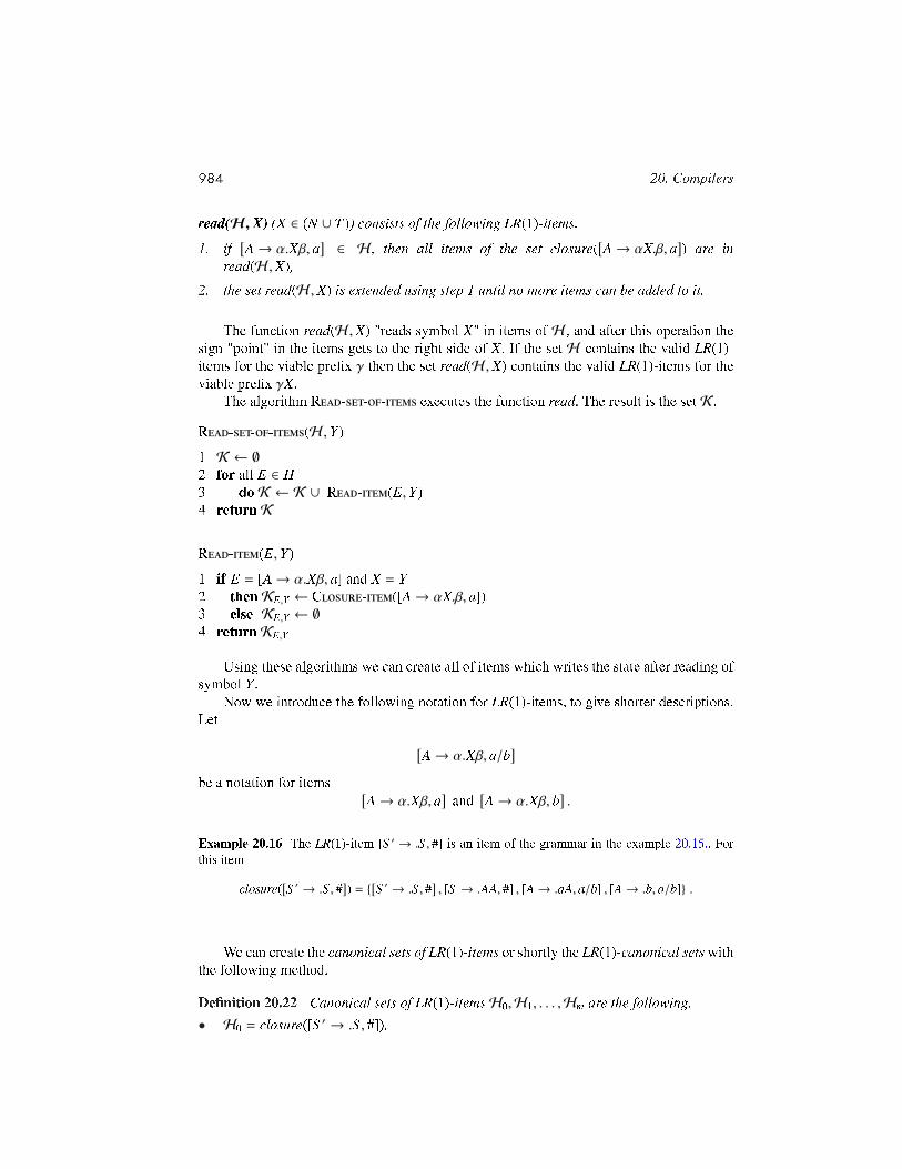
read(H , X) (X ∈ (N ∪ T )) consists of the following LR(1)-items.1. if [A→ α.Xβ, a] ∈ H , then all items of the set closure([A→ αX.β, a]) are in

read(H , X),2. the set read(H , X) is extended using step 1 until no more items can be added to it.

The function read(H , X) "reads symbol X" in items of H , and after this operation thesign "point" in the items gets to the right side of X. If the set H contains the valid LR(1)-items for the viable pre�x γ then the set read(H , X) contains the valid LR(1)-items for theviable pre�x γX.

The algorithm R--- executes the function read. The result is the set K .

R---(H ,Y)1 K ← ∅2 for all E ∈ H3 do K ← K ∪ R-(E,Y)4 return K

R-(E,Y)1 if E = [A→ α.Xβ, a] and X = Y2 then KE,Y ← C-([A→ αX.β, a])3 else KE,Y ← ∅4 return KE,Y

Using these algorithms we can create all of items which writes the state after reading ofsymbol Y .

Now we introduce the following notation for LR(1)-items, to give shorter descriptions.Let

[A→ α.Xβ, a/b]

be a notation for items [A→ α.Xβ, a] and [A→ α.Xβ, b] .

Example 20.16 The LR(1)-item [S ′ → .S , #] is an item of the grammar in the example 20.15.. Forthis item

closure([S ′ → .S , #]) = {[S ′ → .S , #] , [S → .AA, #] , [A→ .aA, a/b] , [A→ .b, a/b]} .

We can create the canonical sets of LR(1)-items or shortly the LR(1)-canonical sets withthe following method.

De�nition 20.22 Canonical sets of LR(1)-itemsH0,H1, . . . ,Hm are the following.• H0 = closure([S ′ → .S , #]),


• Create the set read(H0, X) for a symbol X. If this set is not empty and it is not equal tocanonical setH0 then it is the next canonical setH1.

Repeat this operation for all possible terminal and nonterminal symbol X. If we get anonempty set which is not equal to any of previous sets then this set is a new canoni-cal set, and its index is greater by one as the maximal index of previously generatedcanonical sets.

• repeat the above operation for all previously generated canonical sets and for all sym-bols of the grammar until no more items can be added to it.The sets

H0,H1, . . . ,Hm

are the canonical sets of LR(1)-items of the grammar G.

The number of elements of LR(1)-items for a grammar is �nite, hence the above methodis terminated in �nite time.

The next algorithm creates canonical sets of the grammar G.

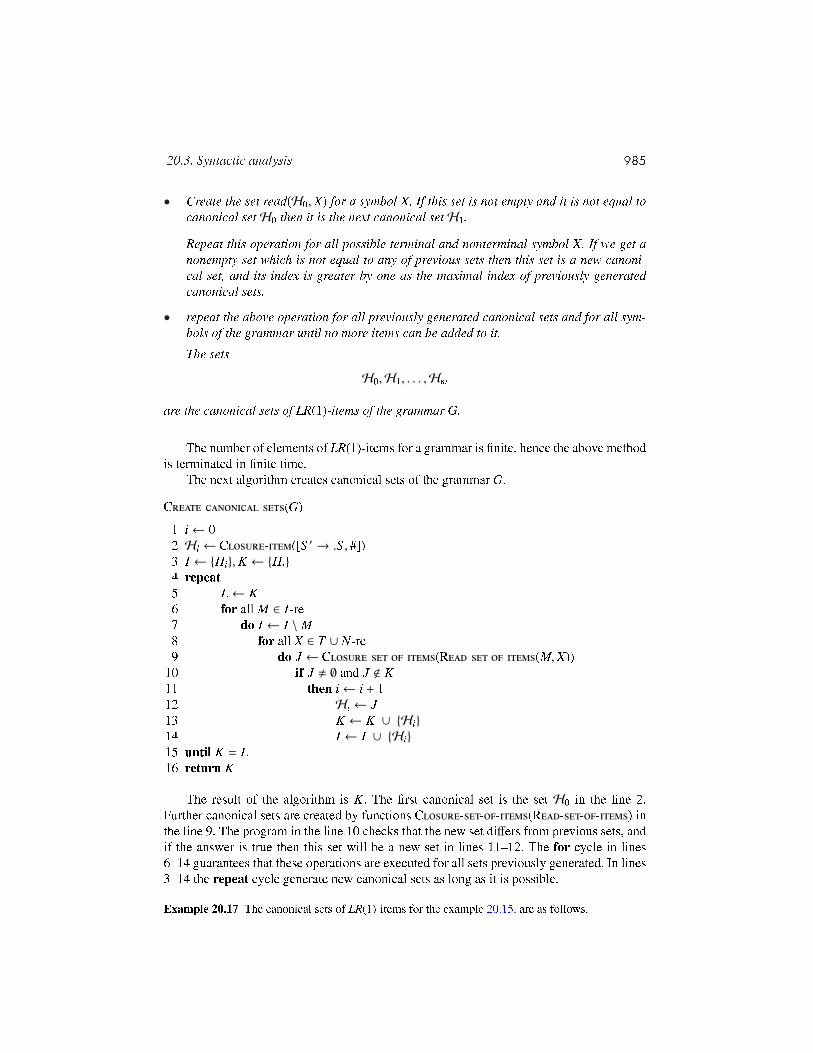
C--(G)1 i← 02 Hi ← C-([S ′ → .S , #])3 I ← {Hi},K ← {Hi}4 repeat5 L← K6 for all M ∈ I-re7 do I ← I \ M8 for all X ∈ T ∪ N-re9 do J ← C---(R---(M, X))

10 if J , ∅ and J < K11 then i← i + 112 Hi ← J13 K ← K ∪ {Hi}14 I ← I ∪ {Hi}15 until K = L16 return K

The result of the algorithm is K. The �rst canonical set is the set H0 in the line 2.Further canonical sets are created by functions C---(R---) inthe line 9. The program in the line 10 checks that the new set differs from previous sets, andif the answer is true then this set will be a new set in lines 11�12. The for cycle in lines6�14 guarantees that these operations are executed for all sets previously generated. In lines3�14 the repeat cycle generate new canonical sets as long as it is possible.

Example 20.17 The canonical sets of LR(1)-items for the example 20.15. are as follows.

986 20. Compilers

GFED@ABC?>=<89:;1 GFED@ABC?>=<89:;5

// GFED@ABC0 A //

a

»»000

0000

0000

0000

0

b

¿¿

S>>}}}}}}}}} GFED@ABC2

A>>}}}}}}}}} a //

b

ÃÃBBB

BBBB

BBGFED@ABC6

a

¯¯A //

b²²

GFED@ABC?>=<89:;9

GFED@ABC?>=<89:;7

GFED@ABC3

a

¯¯A //

b²²

GFED@ABC?>=<89:;8

GFED@ABC?>=<89:;4

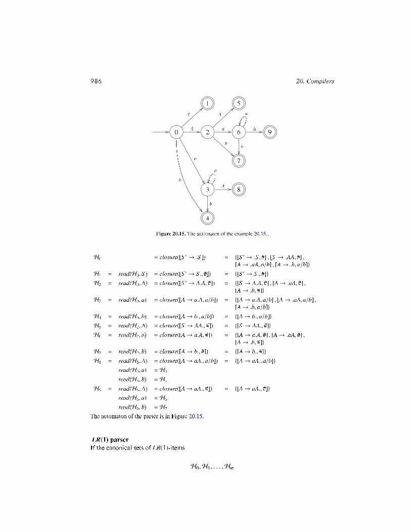
Figure 20.15. The automaton of the example 20.15..

H0 = closure([S ′ → .S ]) = {[S ′ → .S , #] , [S → .AA, #] ,[A→ .aA, a/b] , [A→ .b, a/b]}

H1 = read(H0, S ) = closure([S ′ → S ., #]) = {[S ′ → S ., #]}H2 = read(H0, A) = closure([S ′ → A.A, #]) = {[S → A.A, #] , [A→ .aA, #] ,

[A→ .b, #]}H3 = read(H0, a) = closure([A→ a.A, a/b]) = {[A→ a.A, a/b] , [A→ .aA, a/b] ,

[A→ .b, a/b]}H4 = read(H0, b) = closure([A→ b., a/b]) = {[A→ b., a/b]}H5 = read(H2, A) = closure([S → AA., #]) = {[S → AA., #]}H6 = read(H2, a) = closure([A→ a.A, #]) = {[A→ a.A, #] , [A→ .aA, #] ,

[A→ .b, #]}H7 = read(H2, b) = closure([A→ b., #]) = {[A→ b., #]}H8 = read(H3, A) = closure([A→ aA., a/b]) = {[A→ aA., a/b]}

read(H3, a) = H3

read(H3, b) = H4

H9 = read(H6, A) = closure([A→ aA., #]) = {[A→ aA., #]}read(H6, a) = H6

read(H6, b) = H7

The automaton of the parser is in Figure 20.15.

LR(1) parserIf the canonical sets of LR(1)-items

H0,H1, . . . ,Hm


were created, then assign the state k of an automaton to the set Hk. Relation between thestates of the automaton and the canonical sets of LR(1)-items is stated by the next theorem.This theorem is the �great� theorem of the LR(1)-parsing.

Theorem 20.23 The set of the LR(1)-items being valid for a viable pre�x γ can be assignedto the automaton-state k such that there is path from the initial state to state k labeled bygamma.

This theorem states that we can create the automaton of the parser using canonical sets.Now we give a method to create this LR(1) parser from canonical sets of LR(1)-items.

The deterministic �nite automaton can be described with a table, that is called LR(1)parsing table. The rows of the table are assigned to the states of the automaton.

The parsing table has two parts. The �rst is the action table. Since the operations of par-ser are determined by the symbols of analysed text, the action table is divided into columnslabeled by the terminal symbols. The action table contains information about the action per-forming at the given state and at the given symbol. These actions can be shifts or reductions.The sign of a shift operation is s j, where j is the next state. The sign of the reduction is ri,where i is the serial number of the applied rule. The reduction by the rule having the serialnumber zero means the termination of the parsing and that the parsed text is syntacticallycorrect; for this reason we call this operation accept.

The second part of the parsing table is the goto table. In this table are informationsabout shifts caused by nonterminals. (Shifts belong to terminals are in the action table.)

Let {0, 1, . . . ,m} be the set of states of the automata. The i-th row of the table is �lled infrom the LR(1)-items of canonical setHi.

The i-th row of the action table:• if [A→ α.aβ, b] ∈ Hi and read(Hi, a) = H j then action[i, a] = s j,

• if [A→ α., a] ∈ Hi and A , S ′, then action[i, a] = rl, where A → α is the l-th rule ofthe grammar,

• if [S ′ → S ., #] ∈ Hi, then action[i, #] = accept.The method of �lling in the goto table:

• if read(Hi, A) = H j, then goto[i, A] = j.

• In both table we have to write the text error into the empty positions.

These action and goto tables are called canonical parsing tables.

Theorem 20.24 The augmented grammar G′ is LR(1) grammar iff we can �ll in the par-sing tables created for this grammar without con�icts.

We can �ll in the parsing tables with the next algorithm.

988 20. Compilers

x a y #

parserk

0

X

α

#

¾

6

Figure 20.16. The structure of the LR(1) parser.

F--LR(1)-(G)1 for all LR(1) canonical setsHi2 do for all LR(1)-items3 if [A→ α.aβ, b] ∈ Hi and read(Hi, a) = H j4 then action[i, a] = s j5 if [A→ α., a] ∈ Hi and A , S ′ and A→ α the l-th rule6 then action[i, a] = rl7 if [S ′ → S ., #] ∈ Hi8 then action[i, #] = accept9 if read(Hi, A) = H j

10 then goto[i, A] = j11 for all a ∈ (T ∪ {#})12 do if action[i, a] = �empty�13 then action[i, a]← error14 for all X ∈ N15 do if goto[i, X] = �empty�16 then goto[i, X]← error17 return action, goto

We �ll in the tables its line-by-line. In lines 2�6 of the algorithm we �ll in the actiontable, in lines 9�10 we �ll in the goto table. In lines 11�13 we write the error into thepositions which remained empty.

Now we deal with the steps of the LR(1) parsing. (Figure 20.16).The state of the parsing is written by con�gurations. A con�guration of the LR(1) parser

consists of two parts, the �rst is the stack and the second is the unexpended input text.The stack of the parsing is a double stack, we write or read two data with the operations

push or pop. The stack consists of pairs of symbols, the �rst element of pairs there is aterminal or nonterminal symbol, and the second element is the serial number of the state ofautomaton. The content of the start state is #0.

The start con�guration is (#0, z#), where z means the unexpected text.The parsing is successful if the parser moves to �nal state. In the �nal state the content

of the stack is #0, and the parser is at the end of the text.


Suppose that the parser is in the con�guration (#0 . . . Ykik, ay#). The next move of theparser is determined by action[ik, a].

State transitions are the following.• If action[ik, a] = sl, i.e. the parser executes a shift, then the actual symbol a and the new

state l are written into the stack. That is, the new con�guration is

(#0 . . . Ykik, ay#)→ (#0 . . . Ykikail, y#) .

• If action[ik, a] = rl, then we execute a reduction by the i-th rule A→ α. In this step wedelete |α| rows, i.e. we delete 2|α| elements from the stack, and then we determine thenew state using the goto table. If after the deletion there is the state ik−r at the top of thestack, then the new state is goto[ik−r, A] = il.

(#0 . . . Yk−rik−rYk−r+1ik−r+1 . . . Ykik, y#)→ (#0 . . . Yk−rik−rAil, y#) ,

where |α| = r.• If action[ik, a] = accept, then the parsing is completed, and the analysed text was cor-

rect.• If action[ik, a] = error, then the parsing terminates, and a syntactic error was discovered

at the symbol a.The LR(1) parser is often named canonical LR(1) parser.Denote the action and goto tables together by T . We can give the following algorithm

for the steps of parser.

LR(1)-(xay#,T )1 s← (#0, xay#), s′ ← parsing2 repeat3 s = (#0 . . . Yk−rik−rYk−r+1ik−r+1 . . . Ykik, ay#)4 if action[ik, a] = sl5 then s← (#0 . . . Ykikail, y#)6 else if action[ik, a] = rl and A→ α is the l-th rule and7 |α| = r and goto[ik−r, A] = il8 then s← (#0 . . . Yk−rik−rAil, ay#)9 else if action[ik, a] = accept

10 then s′ ← O.K.11 else s′ ← ERROR12 until s′ = O.K. or s′ = ERROR13 return s′, s

The input parameters of the algorithm are the text xay and table T . The variable s′indicates the action of the parser. It has value parsing in the intermediate states, and itsvalue is O.K. or ERROR at the �nal states. In line 3 we detail the con�guration of the parser,that is necessary at lines 6�8. Using the action table, the parser determines its move fromthe symbol xk at the top of the stack and from the actual symbol a. In lines 4�5 we executea shift step, in lines 6�8 a reduction. The algorithm is completed in lines 9�11. At thismoment, if the parser is at the end of text and the state 0 is at the top of stack, then the

990 20. Compilers

text is correct, otherwise a syntax error was detected. According to this, the output of thealgorithm is O.K. or ERROR, and the �nal con�guration is at the output, too. In the case oferror, the �rst symbol of the second element of the con�guration is the erroneous symbol.

Example 20.18 The action and goto tables of the LR(1) parser for the grammar of example 20.15. areas follows. The empty positions denote errors.

state action gotoa b # S A

0 s3 s4 1 21 accept2 s6 s7 53 s3 s4 84 r3 r35 r16 s6 s7 97 r38 r2 r29 r2

Example 20.19 Using the tables of the previous example, analyse the text abb#.rule

(#0, aab#) s3−→ (#0a3, bb#)s4−→ (#0a3b4, b#)r3−→ (#0a3A8, b#) A→ br2−→ (#0A2, b#) A→ aAs7−→ (#0A2b7, #)r3−→ (#0A2A5, #) A→ br1−→ (#0S 1, #) S → AAelfogad−−−−−→ O.K.

The syntax tree of the sentence is in Figure 20.17.

LALR(1) parserOur goal is to decrease the number of states of the parser, since not only the size but thespeed of the compiler is dependent on the number of states. At the same time, we wish notto cut radically the set of LR(1) grammars and languages, by using our new method.

There are a lot of LR(1)-items in the canonical sets, such that are very similar: their coreare the same, only their lookahead symbols are different. If there are two or more canonicalsets in which there are similar items only, then we merge these sets.

If the canonical setsHi és aH j are mergeable, then let K[i, j] = Hi ∪H j.Execute all of possible merging of LR(1) canonical sets. After renumbering the inde-

xes we obtain sets K0,K1, . . . ,Kn; these are the merged LR(1) canonical sets or LALR(1)


S ′

S

~~~~

~~~~

@@@@

@@@@

A

¡¡¡¡

¡¡¡¡

@@@@

@@@@

A

a A b

b

Figure 20.17. The syntax tree of the sentence aab.

canonical sets.We create the LALR(1) parser from these united canonical sets.

Example 20.20 Using the LR(1) canonical sets of the example 20.17., we can merge the next canoni-cal sets:H3 andH6,H4 andH7,H8 andH9.In the Figure 20.15 it can be seen that mergeable sets are in equivalent or similar positions in the

automaton.

There is no difficulty with the function read if we use merged canonical sets. If

K = H1 ∪H2 ∪ . . . ∪Hk ,

read(H1, X) = H ′1, read(H2, X) = H ′

2, . . . , read(Hk, X) = H ′k ,

andK ′ = H ′

1 ∪H′2 ∪ . . . ∪H

′k ,

thenread(K , X) = K ′ .

We can prove this on the following way. By the de�nition of function read, the setread(H , X) depends on the core of LR(1)-items in H only, and it is independent of thelookahead symbols. Since the cores of LR(1)-items in the setsH1,H2, . . . ,Hk are the same,the cores of LR(1)-items of

read(H1, X), read(H2, X), . . . , read(Hk, X)

are also the same. It follows that these sets are mergeable into a set K ′, thus read(K , X) =

K ′.However, after merging canonical sets of LR(1)-items, elements of this set can raise

992 20. Compilers

difficulties. Suppose thatK[i, j] = Hi ∪H j.• After merging there are not shift-shift con�icts. If

[A→ α.aβ, b] ∈ Hi

and [B→ γ.aδ, c] ∈ H j

then there is a shift for the symbol a and we saw that the function read does not causeproblem, i.e. the set read(K[i, j], a) is equal to the set read(Hi, a) ∪ read(H j, a).

• If there is an item [A→ α.aβ, b]

in the canonical setHi and there is an item[B→ γ., a]

in the set a H j, then the merged set is an inadequate set with the symbol a, i.e. there isa shift-reduce con�ict in the merged set.But this case never happens. Both items are elements of the set Hi and of the set H j.These sets are mergeable sets, thus they are different in lookahead symbols only. Itfollows that there is an item [A→ α.aβ, c] in the set H j. Using the theorem 20.24 weget that the grammar is not a LR(1) grammar; we get shift-reduce con�ict from the setH j for the LR(1) parser, too.

• However, after merging reduce-reduce con�ict may arise. The properties of LR(1) gram-mar do not exclude this case. In the next example we show such a case.

Example 20.21 Let G′ = ({S ′, S , A, B}, {a, b, c, d, e}, P′, S ′) be a grammar, and the derivation rulesare as follows.

S ′ → SS → aAd | bBd | aBe | bAeA→ cB→ c

This grammar is a LR(1) grammar. For the viable pre�x ac the LR(1)-items

{[A→ c., d] , [B→ c., e]} ,for the viable pre�x bc the LR(1)-items

{[A→ c., e] , [B→ c., d]}create two canonical sets.

After merging these two sets we get a reduce-reduce con�ict. If the input symbol is d or e thenthe handle is c, but we cannot decide that if we have to use the rule A → c or the rule B → c forreducing.

Now we give the method for creating a LALR(1) parsing table. First we give the cano-nical sets of LR(1)-items

H1,H2, . . . ,Hm


GFED@ABC?>=<89:;1 GFED@ABC?>=<89:;5

// GFED@ABC0 A //

a

::

b44

S>>}}}}}}}}} GFED@ABC2

A>>||||||||| a //

b ÃÃAAA

AAAA

AAGFED@ABC3,6

a

¯¯A //

b²²

GFED@ABC?>=<89:;8,9

GFED@ABC?>=<89:;4,7

Figure 20.18. The automaton of the example 20.22..

, then we merge canonical sets in which the sets constructed from the core of the items areidentical ones. Let

K1,K2, . . . ,Kn (n ≤ m)

be the LALR(1) canonical sets.For the calculation of the size of the action and goto tables and for �lling in these tables

we use the sets Ki (1 ≤ i ≤ n). The method is the same as it was in the LR(1) parsers. Theconstructed tables are named by LALR(1) parsing tables.

De�nition 20.25 If the �lling in the LALR(1) parsing tables do not produce con�icts thenthe grammar is said to be an LALR(1) grammar.

The run of LALR(1) parser is the same as it was in LR(1) parser.

Example 20.22 Denote the result of merging canonical setsHi andH j byK[i, j]. Let [i, j] be the statewhich belonging to this set.

The LR(1) canonical sets of the grammar of example 20.15. were given in the example 20.17.and the mergeable sets were seen in the example 20.20.. For this grammar we can create the nextLALR(1) parsing tables.

állapot action gotoa b # S A

0 s [3, 6] s [4, 7] 1 21 accept2 s [3, 6] s [4, 7] 5

[3, 6] s [3, 6] s [4, 7] [8, 9][4, 7] r3 r3 r3

5 r1[8, 9] r2 r2 r2

The �lling in the LALR(1) tables are con�ict free, therefore the grammar is an LALR(1) grammar.The automaton of this parser is in Figure 20.18.

Example 20.23 Analyse the text abb# using the parsing table of the previous example.

994 20. Compilers

rule(#0, aab#) s[3,6]−−−−→ (#0a [3, 6] , bb#)

s[4,7]−−−−→ (#0a [3, 6] b [4, 7] , b#)r3−→ (#0a [3, 6] A[8, 9], b#) A→ br2−→ (#0A2, b#) A→ aAs[4,7]−−−−→ (#0A2b [4, 7] , #)r3−→ (#0A2A5, #) A→ br1−→ (#0S 1, #) S → AAelfogad−−−−−→ O.K.

The syntax tree of the parsed text is in the Figure 20.17.

As it can be seen from the previous example, the LALR(1) grammars are LR(1) gram-mars. The converse assertion is not true. In the example 20.21. there is a grammar which isLR(1), but it is not LALR(1) grammar.

Programming languages can be written by LALR(1) grammars. The most frequentlyused methods in compilers of programming languages is the LALR(1) method. The advan-tage of the LALR(1) parser is that the sizes of parsing tables are smaller than the size ofLR(1) parsing tables.

For example, the LALR(1) parsing tables for the Pascal language have a few hundredsof lines, whilst the LR(1) parsers for this language have a few thousands of lines.

Exercises20.3-1 Find the LL(1) grammars among the following grammars (we give their derivationrules only).

1. S → ABcA → a | εB → b | ε

2. S → AbA → a | B | εB → b | ε

3. S → ABBAA → a | εB → b | ε

4. S → aS e | AA → bAe | BB → cBe | d

20.3-2 Prove that the next grammars are LL(1) grammars (we give their derivation rulesonly).

1. S → Bb | CdB → aB | εC → cC | ε

996 20. Compilers

2. S ′ → SS → aAcA | A | BA → b | CeB → dDC → bD → CcS | CcD

20.3-9 Create parsing table for the above LL(1) grammars.20.3-10 Using the recursive descent method, write the parsing program for the above LL(1)grammars.20.3-11 Create canonical sets and the parsing tables for the above LR(1) grammars.20.3-12 Create merged canonical sets and the parsing tables for the above LALR(1) gram-mars.

Problems

20-1. Lexical analysis of a program textThe algorithm L- in the section 20.2 gives a scanner for the text that is describedby only one regular expression or deterministic �nite automaton, i.e. this scanner is ableto analyse only one symbol. Create an automaton which executes total lexical analysis ofa program language, and give the algorithm L-- for this automaton. Letthe input of the algorithm be the text of a program, and the output be the series of symbols.It is obvious that if the automaton goes into a �nite state then its new work begins at theinitial state, for analysing the next symbol. The algorithm �nishes his work if it is at the endof the text or a lexical error is detected.20-2. Series of symbols augmented with data of symbolsModify the algorithm of the previous task on such way that the output is the series of sym-bols augmented with the appropriate attributes. For example, the attribute of a variable is thecharacter string of its name, or the attribute of a number is its value and type. It is practicalto write pointers to the symbols in places of data.20-3. LALR(1) parser from LR (0) canonical setsIf we omit lookahead symbols from the LR(1)-items then we get LR(0)-items. We can de�nefunctions closure and read for LR(0)-items too, doing not care for lookahead symbols. Usinga method similar to the method of LR(1), we can construct LR(0) canonical sets

I0,I1, . . . ,In.

One can observe that the number of merged canonical sets is equal to the number of LR(0)canonical sets, since the cores of LR(1)-items of the merged canonical sets are the same asthe items of the LR(0) canonical sets. Therefore the number of states of LALR(1) parser isequal to the number of states of its LR(0) parser.

Using this property, we can construct LALR(1) canonical sets from LR(0) canonical sets,by completing the items of the LR(0) canonical sets with lookahead symbols. The result ofthis procedure is the set of LALR(1) canonical sets.

It is obvious that the right part of an LR(1)-item begins with symbol point only if this

20. Megjegyzések a fejezethez 997

item was constructed by the function closure. (We notice that there is one exception, the[S ′ → .S ] item of the canonical set H0.) Therefore it is no need for all items of LR(1)canonical sets. Let the kernel of the canonical set H0 be the LR(1)-item [S ′ → .S , #], andlet the kernel of any other canonical set be the set of the LR(1)-items such that there is nopoint at the �rst position on the right side of the item. We give an LR(1) canonical set by itskernel, since all of items can be construct from the kernel using the function closure.

If we complete the items of the kernel of LR(0) canonical sets then we get the kernel ofthe merged LR(1) canonical sets. That is, if the kernel of an LR(0) canonical set is I j, thenfrom it with completions we get the kernel of the LR(1) canonical set, K j.

If we know I j then we can construct read(I j, X) easily. If [B→ γ.Cδ] ∈ I j, C ∗→ Aηand A → Xα, then [A→ X.α] ∈ read(I j, X). For LR(1)-items, if [B→ γ.Cδ, b] ∈ K j,C ∗→ Aη and A → Xα then we have to determine also the lookahead symbols, i.e. thesymbols a such that [A→ X.α, a] ∈ read(K j, X).

If ηδ , ε and a ∈ First(ηδb) then it is sure that [A→ X.α, a] ∈ read(K j, X). In thiscase, we say that the lookahead symbol was spontaneously generated for this item of ca-nonical set read(K j, X). The symbol b do not play important role in the construction of thelookahead symbol.

If ηδ = ε then [A→ X.α, b] is an element of the set read(K j, X), and the lookaheadsymbol is b. In this case we say that the lookahead symbol is propagated from K j into theitem of the set read(K j, X).

If the kernel I j of an LR(0) canonical set is given then we construct the propagatedand spontaneously generated lookahead symbols for items of read(K j, X) by the followingalgorithm.

For all items [B→ γ.δ] ∈ I j we construct the set K j = closure([B→ γ.δ,@]), where

@ is a dummy symbol,• if [A→ α.Xβ, a] ∈ K j and a , @ then [A→ αX.β, a] ∈ read(K j, X) and the symbol a

is spontaneously generated into the item of the set read(K j, X),• if [A→ α.Xβ,@] ∈ K j then [A→ αX.β,@] ∈ read(K j, X), and the symbol @ is pro-

pagated from K j into the item of the set read(K j, X).The kernel of the canonical set K0 has only one element. The core of this element is

[S ′ → .S ]. For this item we can give the lookahead symbol # directly. Since the core of thekernel of all K j canonical sets are given, using the above method we can calculate all ofpropagated and spontaneously generated symbols.

Give the algorithm which constructs LALR(1) canonical sets from LR(0) canonical setsusing the methods of propagation and spontaneously generation.

Chapter notesThe theory and practice of compilers, computers and program languages are of the same age.The construction of �rst compilers date back to the 1950's. The task of writing compilerswas a very hard task at that time, the �rst Fortran compiler took 18 man-years to implement[3]. From that time more and more precise de�nitions and solutions have been given to theproblems of compilation, and better and better methods and utilities have been used in theconstruction of translators.

998 20. Compilers

The development of formal languages and automata was a great leap forward, and wecan say that this development was urged by the demand of writing of compilers. In our daysthis task is a simple routine project. New results, new discoveries are expected in the �eldof code optimisation only.

One of the earliest nondeterministic and backtrack algorithms appeared in the 1960's.The �rst two dynamic programming algorithms were the CYK (Cocke�Younger�Kasami)algorithm from 1965�67 and the Earley-algorithm from 1965. The idea of precedence par-sers is from the end of 1970's and from the beginning of 1980's. The LR(k) grammars wasde�ned by Knuth in 1965; the de�nition of LL(k) grammars is dated from the beginning of1970's. LALR(1) grammars were studied by De Remer in 1971, the elaborating of LALR(1)parsing methods were �nished in the beginning of 1980's [1, 2, 3].

To the middle of 1980's it became obvious that the LR parsing methods are the realefficient methods and since than the LALR(1) methods are used in compilers [1].

A lot of very excellent books deal with the theory and practice of compiles. Perhapsthe most successful of them was the book of Gries [10]; in this book there are interestingresults for precedence grammars. The �rst successful book which wrote about the new LRalgorithms was of Aho and Ullman [2], we can �nd here also the CYK and the Early al-gorithms. It was followed by the "dragon book" of Aho and Ullman[3]; the extended andcorrected issue of it was published in 1986 by authors Aho, Ullman and Sethi [1].

Without completeness we notice the books of Fischer and LeBlanc [8], Tremblay andSorenson [18], Waite and Goos [20], Hunter[12], Pittman [16] and Mak [14]. Advancedachievements are in recently published books, among others in the book of Muchnick [15],Grune, Bal, Jacobs and Langendoen [11], in the book of Cooper and Torczon [6] and in achapter of the book by Louden [13].

There are many books on topics of the theory of formal languages and automata inHungarian. For example the book of Judit Bánkfalvi, Zsolt Bánkfalvi and Gábor Bognárpublished in 1978 [5]. There are books in which a chapter deals with compilers, for examplein the book of Iván Bach [4], Zoltán Fülöp [9], György Révész [17] and László Varga[19], as well as in the electronic course notes of Pál Dömösi, Attila Fazekas, Géza Horváthand Zoltán Mecsei [7]. In [4, 7, 17] the CYK and the Earley algorithms are investigated.About precedence parsers we can read the books [4] and [19]. [4, 5, 9] treat also LR parsingmethods.

Bibliography

[1] A. V. Aho, R. Sethi, J. D. Ullman. Compilers, Principles, Techniques and Tools. Addison-Wesley, 1986. 998[2] A. V. Aho, J. D. Ullman. The Theory of Parsing, Translation and Compiling Vol. I. Prentice-Hall, 1972. 998[3] A. V. Aho, J. D. Ullman. The Theory of Parsing, Translation and Compiling Vol. II. Prentice-Hall, 1973.

997, 998[4] I. Bach. Formális nyelvek (Formal Languages). Typotex, 2001. 998[5] J. Bánkfalvi, Zs. Bánkfalvi, G. Bognár. A formális nyelvek szintaktikus elemzése. Közgazdasági és Jogi

Kiadó, 1978. 998[6] K. D. Cooper, L. Torczon. Engineering a Compiler. Morgan Kaufman Publisher, 2004. 998[7] P. Dömösi, A. Fazekas, G. Horváth, Z. Mecsei. Formális nyelvek és automaták (Formal Languages and Au-

tomaton). Digitális kézirat, 2004. 998[8] C. N. Fischer, R. LeBlanc (szerkeszt�ok). Crafting a Compiler. The Benjamin/Cummings Publishing Com-

pany, 1988. 998[9] Z. Fülöp. Formális nyelvek és szintaktikus elemzésük (Formal Languages and their Syntactical Analysis).

Polygon, 2004 (second edition). 998[10] D. Gries. Compiler Construction for Digital Computers. John Wiley & Sons, 1971. 998[11] D. Grune, H. Bal, C. J. H. Jacobs, K. Langendoen. Modern Compiler Design. John Wiley & Sons, 2000. 998[12] R. W. Hunter. Compilers, Their Design and Construction using Pascal. John Wiley & Sons, 1985. 998[13] K.. Louden. Compilers and interpreters. In A. B. Tucker (szerkeszt�o), Handbook of Computer Science, 99/1�

99/30. o. Chapman & Hall/CRC, 2004. 998[14] R. Mak. Writing Compilers and Interpreters. Addison-Wesley, 1991. 998[15] S. Muchnick. Advanced Compiler Design and Implementation. Morgan Kaufman Publisher, 1997. 998[16] T. Pittman. The Art of Compiler Design, Theory and Practice. Prentice Hall, 1992. 998[17] Gy. Révész. Bevezetés a formális nyelvek elméletébe (Introduction to the Theory of Formal Languages).

Akadémiai Kiadó, 1979. 998[18] J-P. Tremblay, P. G. Sorenson. Compiler Writing. McGraw-Hill Book Co., 1985. 998[19] L. Varga. Rendszerprogramok elmélete és gyakorlata (Theory and Practice of System Programs). Akadémiai

Kiadó, 1980. 998[20] W. Waite, G. Goos. Compiler Construction. Springer-Verlag, 1984. 998

http://blrc.edu.cn/people/Al%20Aho.htm�

http://cm.bell-labs.com/who/ravi/�

http://www-db.stanford.edu/~ullman/�

http://www.aw.com/�



http://vig.prenhall.com/�



http://vig.prenhall.com/�

http://www.typotex.hu/�

http://www.cs.rice.edu/~keith/�

http://www.inf.unideb.hu/~domosi/�

http://www.inf.unideb.hu/~fattila/�

http://www.inf.unideb.hu/~mecseiz/�

http://www.inf.unideb.hu/~mecseiz/hallgato/fonya_OK.pdf�

http://www.aw-bc.com/�

http://www.inf.u-szeged.hu/~fulop/�

http://www.math.u-szeged.hu/polygon/�

http://www.cs.cornell.edu/Info/People/gries/gries.html�

http://www.wiley.com/�

http://www.cs.vu.nl/~bal/�



http://www.cs.sjsu.edu/faculty/louden/�

http://www.bowdoin.edu/~allen/�

http://www.chapmanhall.com/�

http://www.crcpress.com/�

http://www.aw.com/�

http://www.prenhall.com/�

http://www.akkrt.hu/�

http://books.mcgraw-hill.com/�

http://www.akkrt.hu/�

http://www.info.uni-karlsruhe.de/~ggoos/�

http://www.springer.de/ �

Subject Index

A, Áaccept, 969, 987action table, 987, 993actual

symbol, 969, 973algorithms of compilers, 951analyser, 953

lexical, 952, 953semantic, 952, 953, 962syntactic, 952, 953, 962

assembly language program, 954attribute

grammar, 962augmented grammar, 979automaton

deterministic�nite, 956

Bbottom-up parsing, 963

Ccanonical

parser, 989parsing table, 987set

kernel, 997LALR(1), 991LR(0), 996LR(1), 984merged, 991

character stream, 952check, 973closure, 982, 996C-, 983C---, 983code

generator, 952, 954handler, 952optimiser, 952, 954

?C?, 951, 952, 955compilers, 951con�ict

reduce-reduce, 992shift-reduce, 992shift-shift, 992

context dependentgrammar, 962

context freegrammar, 962

C--, 985C--, 975cycle free grammar, 963

Dderivation

leftmost, 964direct, 964

rightmost, 978deterministic

�niteautomaton, 956

directive, 961dynamic semantics, 962

E, Éerror, 969, 987

lexical, 953repair, 952report, 973semantic, 953syntactic, 953, 969, 989

expressionregular, 956

FF--LR(1)-, 988�nal state

parsing, 970�nite

automatondeterministic, 956

F, 967Firstk, 965F, 968Followk, 966

Ggoto table, 987, 993

Subject Index 1001

grammarattribute, 962augmented, 979context dependent, 962context free, 962cycle free, 963LALR(1), 993LL(k), 965LR(1), 981LR(k), 979O-ATG, 952reduced, 963, 973regular, 956two-level, 962unambiguous, 963

Hhandle, 963handler

code, 952list, 952source, 952

I, Íinitial state

parser, 969interpreter, 951

Kkeyword, 959

LLALR(1)

canonical set, 991grammar, 993parser, 952, 990parsing

table, 993leftmost

derivation, 964direct

derivation, 964left to right

parsing, 963lex, 956L-, 958L--, 996lexical

analyser, 952, 953error, 953

list, 952list-handler, 952LL(1) parser, 952LL(1)-, 971LL(1)---, 970LL(k)

grammar, 965lookahead, 960

operator, 960LR(0)

canonical set, 996item, 996

LR(1)canonical set, 984

kernel, 997grammar, 981item, 981

core, 981lookahead symbol, 981valid, 982

parser, 986parsing

table, 987LR(1)-, 989LR(k)

grammar, 979parsing, 979

Mmerged canonical set, 991

O, ÓO-ATG grammar, 952

Pparser, 953, 962

bottom-up, 963canonical, 989�nal state, 970, 988initial state, 969LALR(1), 952left to right, 963LL(1), 952, 969LR(k), 979start con�guration, 988state, 969, 988top-down, 963

parsing, 962table, 969, 987, 993

phrase, 963simple, 963

pop, 969program

assembly language, 954source, 952

language, 951, 952target, 952

language, 951, 952propagation, 997

Rread, 982, 996R-, 984R---, 984R--, 975R--1, 976R--2, 976recursive-descent method, 972reduced grammar, 963, 973reduce-reduce con�ict, 992regular

expression, 956grammar, 956

rightmostderivation, 978substitution, 978

run-time semantics, 962

1002 Subject Index

Sscanner, 952, 953semantic

analyser, 952, 953, 962error, 953

semantics, 962dynamic, 962run-time, 962static, 962

sentence, 963sentential form, 963series of symbols, 953, 955shift-reduce con�ict, 992shift-shift con�ict, 992simple

phrase, 963source

handler, 952language program, 951, 952program, 952

spontaneously generated, 997standard word, 959state

parser, 969static

semantics, 962substitution

rightmost, 978symbol

actual, 969, 973table, 952, 961

syntacticanalyser, 952, 953

analysis, 962error, 953, 969, 989

syntax, 962synthesis, 954

Ttable

parsing, 969, 987, 993target

language program, 951, 952program, 952

top-down parsing, 963two-level grammar, 962

U, Úunambiguous grammar, 963

Vvalid

LR(1)-item, 982viable pre�x, 981

Wwhite space, 956W-, 975

Yyacc, 979

Name index

A, ÁAho, Alfred V., 998, 999

BBach, Iván, 998, 999Bal, Henri E., 998, 999Bánkfalvi, Judit, 998Bánkfalvi, Zsolt, 998Bánkfalvi Judit, 999Bánkfalvi Zsolt, 999Bognár, Gábor, 998, 999

CCocke, J., 998Cooper, Keith D., 998, 999

DDe Remer, F. L., 998Dömösi, Pál, 998, 999

E, ÉEarley, J., 998

FFazekas, Attila, 998, 999Fischer, C. N., 998, 999Fülöp, Zoltán, 998Fülöp Zoltán, 999

GGoos, Gerhard, 998, 999Gries, David, 998, 999Grune, Dick, 998, 999

HHorváth, Géza, 998, 999Hunter, Robin, 998, 999

JJacobs, Ceriel J. H., 998, 999

KKasami, T., 998Knuth, Donald E., 998

LLangendoen, Koen G., 998, 999LeBlanc, R. J., 998, 999Louden, Kenneth C., 998, 999

MMak, Ronald, 998, 999Mecsei, Zoltán, 998, 999Muchnick, Steven S., 998, 999

PPittman, Thomas, 998, 999

RRévész, György, 998, 999

SSethi, Ravi, 998, 999Sorenson, Paul G., 998, 999

TTorczon, Linda, 998, 999Tremblay, Jean-Paul, 998, 999Tucker, Allen B., 999

U, ÚUllman, Jeffrey D., 998Ullman, Jeffrey David, 999

VVarga, László, 998Varga László, 999

1004 Name index

WWaite, William M., 998, 999

YYounger, D. H., 998

Contents

20. Compilers (Zoltán Csörnyei) . . . . . . . . . . . . . . . . . . . . . . . . . . . 95120.1. The structure of compilers . . . . . . . . . . . . . . . . . . . . . . . . . . 95220.2. Lexical analysis . . . . . . . . . . . . . . . . . . . . . . . . . . . . . . . . 955

20.2.1. The automaton of the scanner . . . . . . . . . . . . . . . . . . . . 95620.2.2. Special problems . . . . . . . . . . . . . . . . . . . . . . . . . . . 959

Keywords, standard words . . . . . . . . . . . . . . . . . . . . . . 959Look ahead . . . . . . . . . . . . . . . . . . . . . . . . . . . . . . 960The symbol table . . . . . . . . . . . . . . . . . . . . . . . . . . . 961Directives . . . . . . . . . . . . . . . . . . . . . . . . . . . . . . . 961

20.3. Syntactic analysis . . . . . . . . . . . . . . . . . . . . . . . . . . . . . . . 96220.3.1. LL(1) parser . . . . . . . . . . . . . . . . . . . . . . . . . . . . . . 964

LL(k) grammars . . . . . . . . . . . . . . . . . . . . . . . . . . . . 964Parsing with table . . . . . . . . . . . . . . . . . . . . . . . . . . . 968Recursive-descent parsing method . . . . . . . . . . . . . . . . . . 972

20.3.2. LR(1) parsing . . . . . . . . . . . . . . . . . . . . . . . . . . . . . 978LR(k) grammars . . . . . . . . . . . . . . . . . . . . . . . . . . . 979LR(1) canonical sets . . . . . . . . . . . . . . . . . . . . . . . . . 981LR(1) parser . . . . . . . . . . . . . . . . . . . . . . . . . . . . . 986

LALR(1) parser . . . . . . . . . . . . . . . . . . . . . . . . . . . . 990Bibliography . . . . . . . . . . . . . . . . . . . . . . . . . . . . . . . . . . . . . . 999Subject Index . . . . . . . . . . . . . . . . . . . . . . . . . . . . . . . . . . . . . . 1000Name index . . . . . . . . . . . . . . . . . . . . . . . . . . . . . . . . . . . . . . . 1003

20. compilerscompalg.inf.elte.hu/~tony/informatikai-konyvtar/03... · 2006-05-29 · the task of...

Documents