2. p zambia measurement,levels and trends
TRANSCRIPT

Discussion Draft
34
2. POVERTY IN ZAMBIA:
MEASUREMENT, LEVELS, AND TRENDS
A. Introduction
2.1 This chapter examines poverty—broadly defined as unacceptable deprivation in well-
being—in terms of material deprivation, human deprivation, vulnerability, destitution, and social isolation. It draws on a range of data sources and methods to define the extent of poverty in the state, as well as shed light on recent trends in poverty.
2.2 Poverty cannot be understood in terms of a single indicator or measurement methodology. Consequently, this Assessment takes a multidimensional view of poverty and draws upon a variety of information to analyze the situation faced by the poor in Zambia. The broad definition of poverty used here includes three components – poverty of private resources, poverty of public goods and services, and poverty of relationships. Poverty of private resources
refers to lack of access to both material assets and human capital—health, education, and skills. The poor also suffer from poverty of access to public goods and services like schools, roads, clean water and security. Finally, many of the poor suffer from poverty of social relations and
networks. The very poor often belong to fewer social networks and informal systems of support; some are even isolated from their kinship networks and close family members. All three of these components should be taken into account to fully understand poverty in Zambia. To present a full picture of poverty, this Chapter draws upon both qualitative and quantitative information drawn from both nationally representative household surveys and from in-depth participatory studies. Where possible, comparisons between multiple data sources are made.
B. Self-Assessed Poverty Levels in Zambia
2.3 Perceptions of poverty in Zambia are partially determined by expectations based on past experience. Zambia was once relatively prosperous, with per capita income at the time of independence in 1964 that placed it among the wealthier countries in sub-Saharan Africa. As the price of copper fell beginning in the mid-1970s, the country experienced an almost continuous decline in income per person. Only since 2000 has Zambia experienced consistent growth in income per capita. Because Zambians take past prosperity as a reference point for their standard of living, they overwhelmingly view themselves as poor. Table 2.1, based on the LCMS III, shows 97 percent of rural Zambians and 92 percent of urban Zambians consider themselves either “very poor” or “moderately poor.”

Discussion Draft
35
Table 2.1: Do Zambians Perceive Themselves to Be Poor?
Percentage Distribution of Self-Assessed Poverty Status, 2002-03
Self-Assessed Poverty Status All Zambia Rural Urban
Very Poor (%) 47 52 37
Moderately Poor (%) 48 45 55
Not Poor (%) 5 3 8 Total 100 100 100
Source: 2002-03 LCMS
C. Consumption-Based Poverty Measures: Methodology
2.4 While emphasis is placed in this report on broad measures of poverty, the poverty rates presented here are calculated using consumption data collected in the 2002-03 LCMS. The consumption poverty figures provide a starting point from which to consider the multi-dimensional nature of poverty. This section briefly describes the how the poverty line was determined and used to measure consumption-based poverty rates. A fuller treatment is given in the Annex. The principal steps involved in calculating poverty figures are the following: 1) measure household consumption, 2) adjust for variation in cost of living, 3) determine a poverty line, and 4) calculate a poverty rate. Each of the four steps is explained below.
Measuring Household Consumption
2.5 Households surveyed in the 2002-03 LCMS reported on their levels of consumption of both food and non-food items, including housing. Recorded consumption included purchased items, along with food which the household both produced and consumed. Material consumed was valued at local prices (collected in a separate price survey at markets in district centers), and all consumption was added up to produce a total value of consumption for the household.16
2.6 The poverty analysis was conducted using each household’s level of consumption per adult equivalent rather than consumption per person. Consumption per adult equivalent for each household was calculated by dividing the household’s total consumption by the number of adult equivalents in each household. In calculating adult equivalents, adults each counted as one, while each child counted as a fraction of an adult equivalent, with the exact figure depending on age. The lower adult equivalent values for children reflects the lower calorie needs of children. In terms of how much consumption is needed to meet basic needs, a young child is “equivalent” to less than one adult.
16 Purchases of durable goods, i.e. those that are used over a long period of time, are not included in the consumption aggregate, and instead a “durable good user fee” is calculated for households that own such goods. Also, housing costs are imputed for most households. See the Annex for details.

Discussion Draft
36
Box 2.1: Why Measure Poverty with Consumption and Not Simply
Expenditure or Income?
A household’s consumption is equal to the sum of (1) expenditures plus (2) the value of home-produced food. Expenditure rather than income is used for the first half of the calculation for two reasons. First, household surveys measure what people spend more accurately than their incomes. Second, income is typically variable over the course of the year, so expenditure provides a better measure of welfare over time. Consumption is a better measure of welfare than simple expenditure alone, because much of what many households consume is their own production, which would not be captured by expenditure. Ignoring home-produced food would greatly understate the consumption levels of rural households
Adjust for Variation in Cost of Living
2.7 Because there is wide variation in the cost of living across space in Zambia, it was necessary to adjust the value of household consumption using a price index. This price index was calculated using local price data collected as part of the LCMS. The index also corrects for variation in prices over the 12 months during which the survey data was collected.17
Determine a Poverty Line
2.8 This is the key step in the process. The notion of a poverty line is conceptually rooted in a “standard of living.” The poverty line is the minimum level of consumption below which people are unable to meet their basic needs for food, housing, and everything else. There is no single correct poverty line, and any poverty line necessarily reflects some measure of judgment about what “basic needs” entails in a particular society. The procedure used to estimate the poverty line here follows the procedure used in a variety of other developing countries:
Choose a level for minimum food calorie needs. Minimum calories per adult were taken as 2464 per day, as per guidelines from the World Health Organization (1985). Determine the composition of food basket for a typical household near poverty line.
Average shares of consumption in different foods were determined for households that ranked in the middle fifth (quintile) of all households nationally. Calculate cost of meeting calorie needs with that food basket. The cost of reaching 2464 calories with the food basket was found to be 52843 Kwacha per month, at national median prices. This is the core or food poverty line, i.e. the minimum consumption level of food required to meet basic food needs alone. Add additional amount for non-food consumption. Because basic needs entail more than food, the poverty line should reflect non-food as well as food needs. Like the food basket shares, the non-food share was determined by examining the consumption patterns of a typical household near the poverty line. Specifically, it was found that for the average household in the middle quintile of all households nationally, 28 percent of its consumption was for non-food items. The total poverty line was then calculated by adding a corresponding percentage to the food poverty
17 Cost-of-living adjustments for both urban and rural households were done using price data collected at markets at district centers, which are generally urban. Consequently, the price index does not reflect differences in prices between urban and rural areas within districts. According to CSO personnel, in many areas district centers are the only locations with active markets, so prices for district centers may in fact represent the most relevant market prices for households in the district. Assuming that spatial price variation is chiefly between rather than within districts, this shortcoming in the price index probably has minimal impact on the analysis presented here.

Discussion Draft
37
line.18 The total poverty line, which is the minimum monthly consumption needed to satisfy basic food and non-food needs, was found to be 73394 Kwacha per adult. The total poverty line is referred to throughout the text as simply the “poverty line.”
2.9 At official exchange rates in mid-2003, the poverty line is equal to approximately $US15 per adult per month, or US$0.50 per adult per day. For a typical family of six, the poverty line amounts to about 350,000 Kwacha per month.19
2.10 The food basket used for the poverty line calculation reflects the diet of a typical poor person in Zambia. A poor person gets 70 percent of his or her calories from grains, chiefly various forms of maize, and most of the remainder from vegetables. The daily food consumption of a poor Zambian adult with consumption level at the core poverty line would be roughly as follows:20
2-3 plates of nshima a medium-sized vegetable such as a sweet potato or tomato a few spoonfuls of oil every 3-4 days, a small serving of chicken, beef, or fish every 3-4 days, a piece of fruit such as a banana or mango a handful of groundnuts a couple teaspoons of sugar
Calculate Poverty Rates
2.11 Once the poverty line is determined and consumption per adult equivalent calculated for each household, estimating poverty rates is straightforward. The most common measure is the poverty headcount, which is simply the fraction of individuals with levels of consumption below the poverty line. In addition to the headcount, two other consumption poverty measures were estimated. The poverty gap index expresses the average gap between the consumption of the poor and the poverty line. The poverty gap index is higher not just when there are more people but also when consumption levels are lower among the poor. The poverty severity index is similar to the poverty gap index but gives greater weight to the very poorest individuals.
2.12 Poverty rates are also calculated using both the poverty line and the lower food or core poverty line. The use of two poverty cutoffs provides some indication of the sensitivity of poverty measures to the poverty line.
18 Specifically, the food poverty line was multiplied by 1/(1-0.28). 19 This figure was calculated using the adult equivalent scale for a “typical” family of six consisting of two adults, and one child in each of 4 age categories: 1-2, 3-5, 7-10, and 10-12. 20 The food basket underlying the poverty line consists of 44 items, reflecting the much wider variation in foods consumed across the whole country than is consumed by a typical individual. This stylized food basket was determined by scaling the poverty-line food basket down to the food consumption level of someone with total consumption at the core poverty level, grouping the foods into major categories, adding up the basket’s food quantities by weight in those categories, and then determining corresponding quantities among the most common foods.

Discussion Draft
38
Box 2.2: How Can the Core Poverty Line Be Interpreted?
Like many other poverty studies, this analysis defines both a total poverty line and a core poverty line equal to the food poverty line. A problem with the idea of a core poverty line (also sometimes called the food poverty line or the extreme poverty line) is that core poverty does not correspond to any underlying welfare concept. It is simply a lower line, without any clear basis. It is sometimes referred to as the minimum expenditure required to meet basic food needs. However, this is a misleading interpretation. Because some non-food consumption is a part of basic needs and all individuals will have some non-food consumption, someone with total consumption equal to the food poverty line is not meeting his or her basic food needs.
An alternative core poverty line could be constructed by revisiting the underlying calorie requirement. The calorie requirement used here is taken from the WHO’s recommended calorie intakes. An alternative core poverty line could reasonably be constructed with food and non-food components, but basing the food component on a calorie requirement of, for example, 70-80% of the WHO’s recommended calories.
It is also possible to interpret the usual core poverty line as if it were a basic poverty line calculated from a lower calorie requirement. Given the mathematics of the poverty line calculations and the particular non-food consumption share in Zambia, the core poverty line used in this report is equal to a total poverty line (with food and non-food components) based on a calorie requirement of 72% of the WHO’s recommendations. This lower calorie requirement amounts to 1774 calories per adult and correspondingly lower figures for children. This is similar to the lower calorie requirements used in some poverty studies and sometimes associated with “minimum” calorie requirements rather than the WHO’s more generous “recommended” calories. Thus the core poverty rates in this paper can be viewed as poverty rates which account for both food and non-food needs but assume a lower calorie requirement. This provides an alternative way of interpreting the core poverty figures.
Poverty Measures
2.13 Using the poverty line and core poverty line described in the previous section, the national headcount estimates are 56 percent for poverty and 36 percent for core poverty. In other words, over half of Zambians have levels of consumption that are insufficient to meet basic needs, and more than a third have consumption levels that would be inadequate to meet basic food needs alone, even if they were able to forego all non-food consumption. Table 2.2 shows poverty and core poverty rates for urban and rural households separately. Poverty rates are highest in rural areas where two-thirds of Zambia’s population resides. Consequently, the poor are highly concentrated in rural areas. Seventy-two percent of the poor live in rural zones.

Discussion Draft
39
Table 2.2: Headcount Poverty Estimates, 2002-03
National Rural Urban
Below Poverty Line (%) 56 62 45 Below Core Poverty Line (%) 36 40 28
Source: Analysis of 2002-03 LCMS
Figure 2.1: Where are the Poor?
Percentages of Nation’s Poor Living in Urban and Rural Areas
28%
72%
Urban
Rural
2.14 The urban population of Zambia is found mainly in Copperbelt and Lusaka provinces, which are home to 69% of urban Zambians. The remaining seven provinces are overwhelmingly rural. Poverty is lowest in Southern and Lusaka provinces, which both have headcount poverty rates of 47%. Poverty rates are highest in the most northerly provinces: Northern, Luapula, and Northwestern.

Discussion Draft
40
Figure 2.2: Poverty Headcount by Province
2.15 Figure 2.3 show a breakdown of the location of the poor by province. The largest fraction of the poor on a national basis—17 percent—is found in Northern, which is also the province with the highest poverty headcount rate. Although Lusaka and Copperbelt have relatively low poverty rates, they also have large populations. Consequently, they are home to large fractions of the country’s poor.
Figure 2.3: Where are the Poor? Distribution of Poor by Province
Northwestern: 6%
Wes tern: 7%
Luapula: 9%
Southern: 10%
Centra l: 10%
Lusaka: 12%
Eastern: 13%
Copperbelt: 15%
Northern: 17%
y
200 0 200 400 Miles
N
EW
S
y y
Poverty Headcount0.470.47 - 0.560.56 - 0.670.67 - 0.75
47% 47-56% 56-67%
67-75%

Discussion Draft
41
D. Central Statistical Office Consumption-Based Poverty Figures
2.16 There is an internal debate in Zambia about the levels of poverty. In analyzing the same LCMS data used here, the Zambia Central Statistical Office (CSO) implemented a similar methodology to that described above, but with a number of minor variations. CSO made slightly different choices for its food basket, minimum calorie requirements, adult equivalent definition, and price index. Further details are presented in the Annex. As a consequence of these differences, CSO finds higher poverty rates, e.g. a national headcount of 67 percent compared to the 56 percent found using the methodology in this report. It is important to note that the differences in methodology are relatively minor, and that the differences in poverty estimates are largely inconsequential. The ranking of subpopulation and the overall profile of both urban and rural poverty in this report differs little from what is presented in CSO’s own analysis of the survey data, CSO (2004). The small differences in poverty point estimates should not distract from the larger picture of poverty in Zambia, which is largely the same whether one uses CSO’s figures or those in this report.
2.17 The headcount poverty estimates from this report (“PVA estimates”) are shown side by side along with the CSO estimates in Table 2.3. Also shown are the ranking by province in terms of headcount. While there are some differences in provincial rank between the two sets of estimates, the overall differences are small. Both the PVA and CSO estimates show that the poorest areas are Northern, Luapula, Northwestern, and Eastern provinces while the least poor are Copperbelt, Lusaka, and Southern provinces.
2.18 The Jesuit Centre for Theological Reflection (JCTR), a prominent non-governmental organization in Lusaka, monitors the monthly price of a Basic Needs Basket which represents the cost of living for a family of six in Lusaka and other urban areas. The cost of the basket includes a much larger cost for housing than that used for the analysis presented here. Consequently, taking the JCTR cost of living as a poverty line would imply higher poverty rates than those presented here.
Table 2.3: 2002-03 Headcount Poverty Estimates Compared to CSO Estimates
PVA
Estimates
CSO Estimates Province
Rank (PVA)
Province
Rank (CSO)
Province
Central 54 69 5 5
Copperbelt 52 58 7 8
Eastern 56 71 4 3
Luapula 67 70 2 4
Lusaka 47 57 8 9
Northern 75 81 1 1
Northwestern 61 72 3 2
Southern 47 63 9 7
Western 52 65 6 6
All Zambia 56 67
Rural 62 74
Urban 45 52
Source: 2002-03 LCMS
Discussion Draft
42
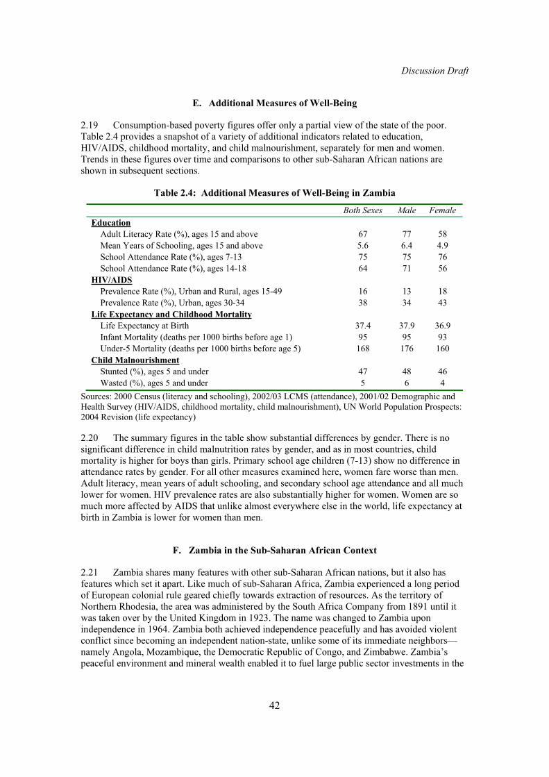
E. Additional Measures of Well-Being
2.19 Consumption-based poverty figures offer only a partial view of the state of the poor. Table 2.4 provides a snapshot of a variety of additional indicators related to education, HIV/AIDS, childhood mortality, and child malnourishment, separately for men and women. Trends in these figures over time and comparisons to other sub-Saharan African nations are shown in subsequent sections.
Table 2.4: Additional Measures of Well-Being in Zambia
Both Sexes Male Female
Education
Adult Literacy Rate (%), ages 15 and above 67 77 58
Mean Years of Schooling, ages 15 and above 5.6 6.4 4.9
School Attendance Rate (%), ages 7-13 75 75 76
School Attendance Rate (%), ages 14-18 64 71 56
HIV/AIDS
Prevalence Rate (%), Urban and Rural, ages 15-49 16 13 18
Prevalence Rate (%), Urban, ages 30-34 38 34 43
Life Expectancy and Childhood Mortality
Life Expectancy at Birth 37.4 37.9 36.9
Infant Mortality (deaths per 1000 births before age 1) 95 95 93
Under-5 Mortality (deaths per 1000 births before age 5) 168 176 160
Child Malnourishment
Stunted (%), ages 5 and under 47 48 46
Wasted (%), ages 5 and under 5 6 4
Sources: 2000 Census (literacy and schooling), 2002/03 LCMS (attendance), 2001/02 Demographic and Health Survey (HIV/AIDS, childhood mortality, child malnourishment), UN World Population Prospects: 2004 Revision (life expectancy)
2.20 The summary figures in the table show substantial differences by gender. There is no significant difference in child malnutrition rates by gender, and as in most countries, child mortality is higher for boys than girls. Primary school age children (7-13) show no difference in attendance rates by gender. For all other measures examined here, women fare worse than men. Adult literacy, mean years of adult schooling, and secondary school age attendance and all much lower for women. HIV prevalence rates are also substantially higher for women. Women are so much more affected by AIDS that unlike almost everywhere else in the world, life expectancy at birth in Zambia is lower for women than men.
F. Zambia in the Sub-Saharan African Context
2.21 Zambia shares many features with other sub-Saharan African nations, but it also has features which set it apart. Like much of sub-Saharan Africa, Zambia experienced a long period of European colonial rule geared chiefly towards extraction of resources. As the territory of Northern Rhodesia, the area was administered by the South Africa Company from 1891 until it was taken over by the United Kingdom in 1923. The name was changed to Zambia upon independence in 1964. Zambia both achieved independence peacefully and has avoided violent conflict since becoming an independent nation-state, unlike some of its immediate neighbors—namely Angola, Mozambique, the Democratic Republic of Congo, and Zimbabwe. Zambia’s peaceful environment and mineral wealth enabled it to fuel large public sector investments in the
Discussion Draft
43
1960s and 70s, but the subsequent decline in the international price of copper has caused per capita income to drop precipitously. Although the country’s economy outranked its neighbors immediately after independence, it is now among the poorer states on the continent.
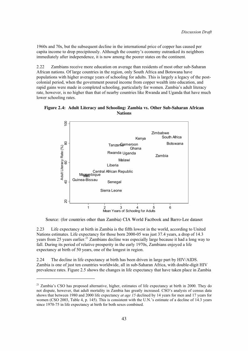
2.22 Zambians receive more education on average than residents of most other sub-Saharan African nations. Of large countries in the region, only South Africa and Botswana have populations with higher average years of schooling for adults. This is largely a legacy of the post-colonial period, when the government poured income from copper wealth into education, and rapid gains were made in completed schooling, particularly for women. Zambia’s adult literacy rate, however, is no higher than that of nearby countries like Rwanda and Uganda that have much lower schooling rates.
Figure 2.4: Adult Literacy and Schooling: Zambia vs. Other Sub-Saharan African
Nations
BotswanaCameroon
Central African Republic
Ghana
Guinea-Bissau
Kenya
Liberia
Malawi
MaliMozambique
Rwanda
Senegal
Sierra Leone
South Africa
Tanzania
UgandaZambia
Zimbabwe
20
40
60
80
100
Adult L
itera
cy R
ate
(%
)
1 2 3 4 5 6Mean Years of Schooling for Adults
Source: (for countries other than Zambia) CIA World Factbook and Barro-Lee dataset
2.23 Life expectancy at birth in Zambia is the fifth lowest in the world, according to United Nations estimates. Life expectancy for those born 2000-05 was just 37.4 years, a drop of 14.3 years from 25 years earlier.21 Zambians decline was especially large because it had a long way to fall. During its period of relative prosperity in the early 1970s, Zambians enjoyed a life expectancy at birth of 50 years, one of the longest in region.
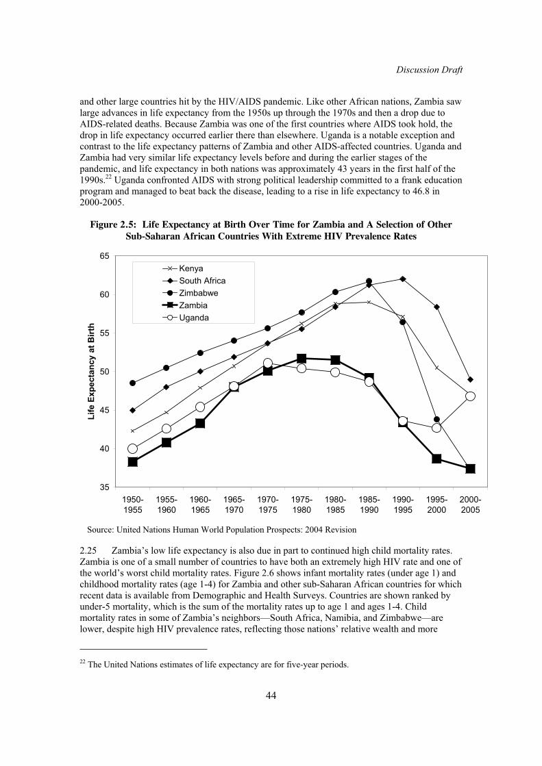
2.24 The decline in life expectancy at birth has been driven in large part by HIV/AIDS. Zambia is one of just ten countries worldwide, all in sub-Saharan Africa, with double-digit HIV prevalence rates. Figure 2.5 shows the changes in life expectancy that have taken place in Zambia
21 Zambia’s CSO has proposed alternative, higher, estimates of life expectancy at birth in 2000. They do not dispute, however, that adult mortality in Zambia has greatly increased. CSO’s analysis of census data shows that between 1980 and 2000 life expectancy at age 15 declined by 14 years for men and 17 years for women (CSO 2003, Table 4, p. 145). This is consistent with the U.N.’s estimate of a decline of 14.3 years since 1970-75 in life expectancy at birth for both sexes combined.
Discussion Draft
44
and other large countries hit by the HIV/AIDS pandemic. Like other African nations, Zambia saw large advances in life expectancy from the 1950s up through the 1970s and then a drop due to AIDS-related deaths. Because Zambia was one of the first countries where AIDS took hold, the drop in life expectancy occurred earlier there than elsewhere. Uganda is a notable exception and contrast to the life expectancy patterns of Zambia and other AIDS-affected countries. Uganda and Zambia had very similar life expectancy levels before and during the earlier stages of the pandemic, and life expectancy in both nations was approximately 43 years in the first half of the 1990s.22 Uganda confronted AIDS with strong political leadership committed to a frank education program and managed to beat back the disease, leading to a rise in life expectancy to 46.8 in 2000-2005.
Figure 2.5: Life Expectancy at Birth Over Time for Zambia and A Selection of Other
Sub-Saharan African Countries With Extreme HIV Prevalence Rates
35
40
45
50
55
60
65
1950-
1955
1955-
1960
1960-
1965
1965-
1970
1970-
1975
1975-
1980
1980-
1985
1985-
1990
1990-
1995
1995-
2000
2000-
2005
Lif
e E
xp
ecta
ncy
at
Bir
th
Kenya
South Africa
Zimbabwe
Zambia
Uganda
Source: United Nations Human World Population Prospects: 2004 Revision
2.25 Zambia’s low life expectancy is also due in part to continued high child mortality rates. Zambia is one of a small number of countries to have both an extremely high HIV rate and one of the world’s worst child mortality rates. Figure 2.6 shows infant mortality rates (under age 1) and childhood mortality rates (age 1-4) for Zambia and other sub-Saharan African countries for which recent data is available from Demographic and Health Surveys. Countries are shown ranked by under-5 mortality, which is the sum of the mortality rates up to age 1 and ages 1-4. Child mortality rates in some of Zambia’s neighbors—South Africa, Namibia, and Zimbabwe—are lower, despite high HIV prevalence rates, reflecting those nations’ relative wealth and more
22 The United Nations estimates of life expectancy are for five-year periods.

Discussion Draft
45
sophisticated health infrastructure. In contrast, a child’s odds of survival in Zambia are among the lowest in Africa. Ninety-five out of 1000 Zambian children do not survive past their 1st year, and an additional 80 die before reaching age five.
Figure 2.6: Child Mortality Rates for Sub-Saharan African Countries
0 50 100 150 200 250
South Africa 1998
Namibia 2000
Gabon 2000
Eritrea 2002
Madagascar 2003/2004
Zimbabwe 1999
Mauritania 2000/01
Ghana 2003
Kenya 2003
Nigeria 1999
Togo 1998
Tanzania 1999
Cameroon 1998
Uganda 2000/01
Benin 2001
Ethiopia 2000
Zambia 2001/02
Cote d'Ivoire 1998/99
Burkina Faso 2003
Malawi 2000
Rwanda 2000
Mali 2001
Niger 1998
Deaths per 1000 Births
Infant (Under Age 1) Mortality
Childhood (Age 1-4) Mortality
Source: Demographic and Health Surveys Note: The sum of the two bars is equal to the under-5 mortality rate.
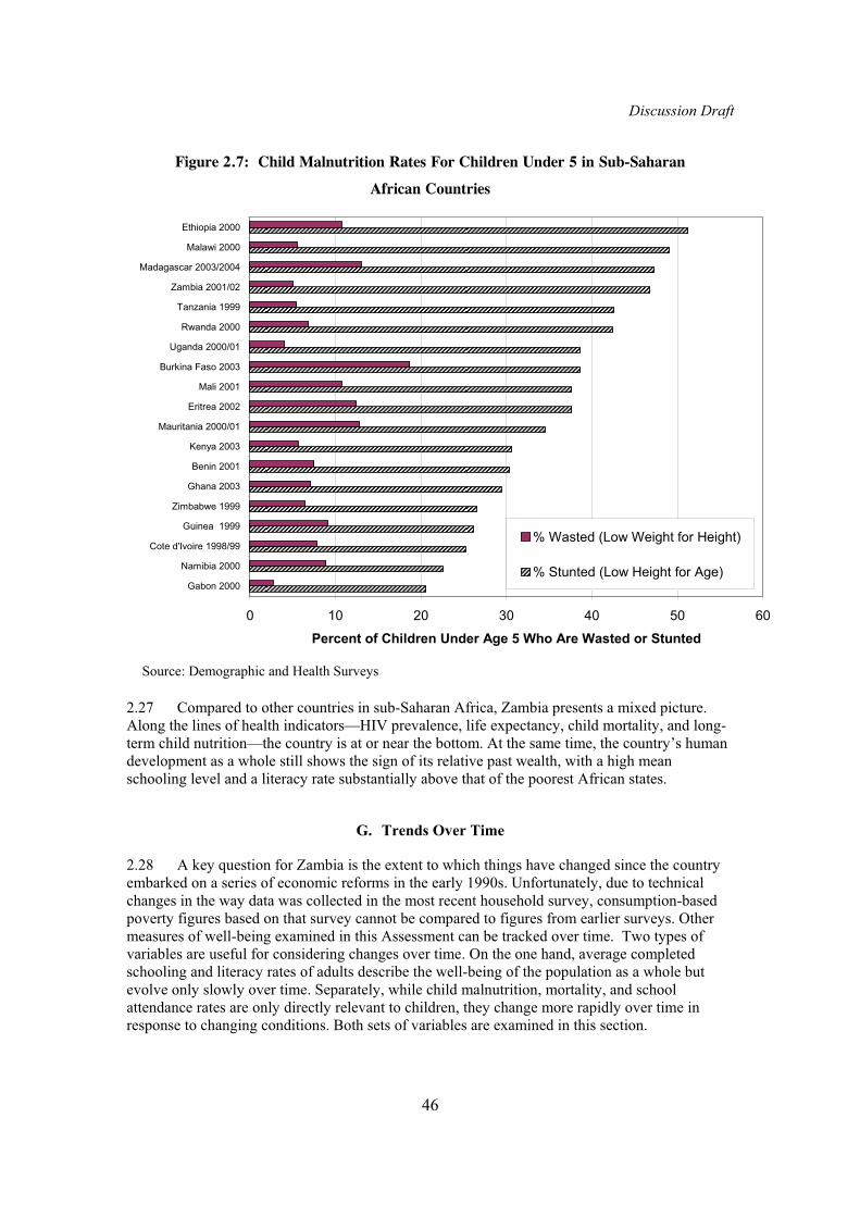
2.26 Another way to compare welfare across countries is by examining child nutrition outcomes. There are two indicators typically used: wasting and stunting. A “stunted” child is substantially below normal height-for-age while a child who is “wasted” is substantially below normal weight-for-height.23 Stunting generally indicates chronic, long-term malnutrition and disease, while wasting is associated with more recent hunger. Zambia’s rate of stunting for children under age five is 46.8 percent, one of the highest among sub-Saharan African countries for which data is available. The percentage of Zambian children that were wasted in 2001-02 is 5 percent, which is relatively low for the region.
23 Specifically, a child is considered wasted or stunted if he or she is more than 2 standard deviations below the norm for a reference population.
Discussion Draft
46
Figure 2.7: Child Malnutrition Rates For Children Under 5 in Sub-Saharan
African Countries
0 10 20 30 40 50 60
Gabon 2000
Namibia 2000
Cote d'Ivoire 1998/99
Guinea 1999
Zimbabwe 1999
Ghana 2003
Benin 2001
Kenya 2003
Mauritania 2000/01
Eritrea 2002
Mali 2001
Burkina Faso 2003
Uganda 2000/01
Rwanda 2000
Tanzania 1999
Zambia 2001/02
Madagascar 2003/2004
Malawi 2000
Ethiopia 2000
Percent of Children Under Age 5 Who Are Wasted or Stunted
% Wasted (Low Weight for Height)
% Stunted (Low Height for Age)
Source: Demographic and Health Surveys
2.27 Compared to other countries in sub-Saharan Africa, Zambia presents a mixed picture. Along the lines of health indicators—HIV prevalence, life expectancy, child mortality, and long-term child nutrition—the country is at or near the bottom. At the same time, the country’s human development as a whole still shows the sign of its relative past wealth, with a high mean schooling level and a literacy rate substantially above that of the poorest African states.
G. Trends Over Time
2.28 A key question for Zambia is the extent to which things have changed since the country embarked on a series of economic reforms in the early 1990s. Unfortunately, due to technical changes in the way data was collected in the most recent household survey, consumption-based poverty figures based on that survey cannot be compared to figures from earlier surveys. Other measures of well-being examined in this Assessment can be tracked over time. Two types of variables are useful for considering changes over time. On the one hand, average completed schooling and literacy rates of adults describe the well-being of the population as a whole but evolve only slowly over time. Separately, while child malnutrition, mortality, and school attendance rates are only directly relevant to children, they change more rapidly over time in response to changing conditions. Both sets of variables are examined in this section.

Discussion Draft
47
2.29 At the macro level, the economy has finally emerged from a period of great instability and achieved stable but modest growth. The economy experienced severe declines in the first years after the implementation of reforms. Output per capita declined by 11 percent in 1994 and a further 5 percent in 1995. (The pattern of growth since 1991 is examined in more detail in Chapter 3.) Evidence does suggest that the reforms set the stage for later growth. In recent years, Zambia has experienced its longest period of sustained growth since independence, averaging 2 percent annual GDP per capita growth 2000-2003. Given the rocky pattern of growth at the aggregate level that Zambia experienced during the 1990s, it would be surprising if there had been substantial improvements in human welfare on average over that period. Indeed, most welfare indicators show only small changes over the course of the decade.
Figure 2.8: GDP Per Capita, Levels and Annual Growth Rates
-15
-10
-5
0
5
10
15
20
25
196
0
196
2
196
4
196
6
196
8
197
0
197
2
197
4
197
6
197
8
198
0
198
2
198
4
198
6
198
8
199
0
199
2
199
4
199
6
199
8
200
0
200
2
Year
% A
nn
ual
Ch
an
ge
0
50
100
150
200
250
300
350
400
450
500
GD
P p
er
Cap
ita (
Th
ou
san
ds o
f
19
94 K
wa
ch
a)
Annual Growth Rate of GDP per Capita (left scale) GDP per Capita (right scale)
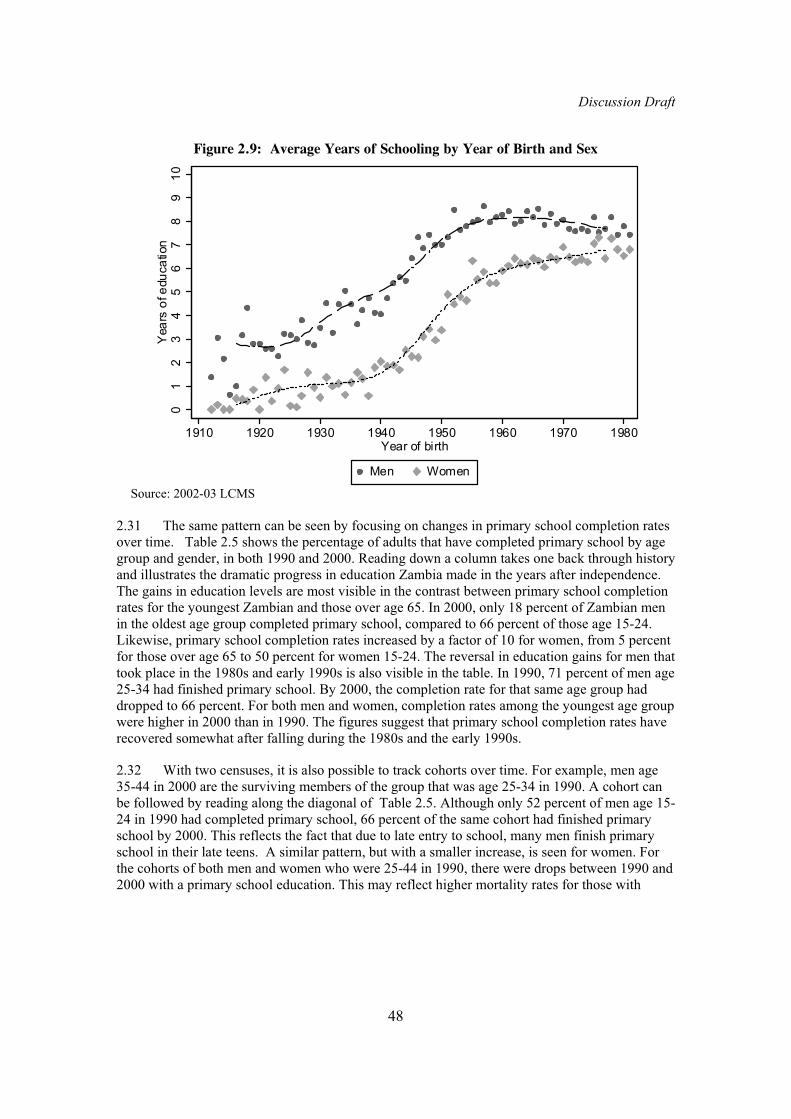
Source: IMF
2.30 Over the course of the post-independence period, there were large advances in education levels, and gains were particularly rapid for women. Average years of education by sex and year of birth are shown in Figure 2.9. The average Zambian woman born in 1940 received just over one year of schooling, while women born in 1960 averaged over six years of education. Later cohorts of women showed continued modest gains, but average education levels for men have
declined slightly. Overall, forward progress on education has stagnated since Zambia’s economic woes intensified in the 1970s.
Discussion Draft
48
Figure 2.9: Average Years of Schooling by Year of Birth and Sex
01
23
45
67
89
10
Yea
rs o
f e
du
ca
tion
1910 1920 1930 1940 1950 1960 1970 1980Year of birth
Men Women
Source: 2002-03 LCMS
2.31 The same pattern can be seen by focusing on changes in primary school completion rates over time. Table 2.5 shows the percentage of adults that have completed primary school by age group and gender, in both 1990 and 2000. Reading down a column takes one back through history and illustrates the dramatic progress in education Zambia made in the years after independence. The gains in education levels are most visible in the contrast between primary school completion rates for the youngest Zambian and those over age 65. In 2000, only 18 percent of Zambian men in the oldest age group completed primary school, compared to 66 percent of those age 15-24. Likewise, primary school completion rates increased by a factor of 10 for women, from 5 percent for those over age 65 to 50 percent for women 15-24. The reversal in education gains for men that took place in the 1980s and early 1990s is also visible in the table. In 1990, 71 percent of men age 25-34 had finished primary school. By 2000, the completion rate for that same age group had dropped to 66 percent. For both men and women, completion rates among the youngest age group were higher in 2000 than in 1990. The figures suggest that primary school completion rates have recovered somewhat after falling during the 1980s and the early 1990s.
2.32 With two censuses, it is also possible to track cohorts over time. For example, men age 35-44 in 2000 are the surviving members of the group that was age 25-34 in 1990. A cohort can be followed by reading along the diagonal of Table 2.5. Although only 52 percent of men age 15-24 in 1990 had completed primary school, 66 percent of the same cohort had finished primary school by 2000. This reflects the fact that due to late entry to school, many men finish primary school in their late teens. A similar pattern, but with a smaller increase, is seen for women. For the cohorts of both men and women who were 25-44 in 1990, there were drops between 1990 and 2000 with a primary school education. This may reflect higher mortality rates for those with

Discussion Draft
49
HIV/AIDS. Urban residents are more than twice as likely to be infected with HIV and also much more likely to have completed primary school.24
Table 2.5: How Have Primary School Completion Rates Changed Over Time?
Percentages Finishing Primary School by Age Group and Sex, 1990 and 2000
Age Group Men 1990 Men 2000 Women 1990 Women 2000
15-24 52 56 48 50
25-34 71 66 49 50
35-44 63 67 28 44
45-54 35 58 9 26
55-64 18 34 6 9
65+ 11 18 6 5
All adults 52 57 37 43
Source: 1990 and 2000 Censuses
2.33 Another way to track the evolution of human capital over time is to examine changes in literacy by age group. Literacy figures from both the 2000 Census and the most recent
Demographic and Health Survey are shown in Figure 2.10. Although the DHS and the census collect literacy information in very different ways, the two series are similar, except that the DHS shows higher rates of literacy for older men.25 Both show that literacy rates are roughly unchanged for adult women up to age 44 and that they have declined in recent generations of adult men.
24 It is not possible to examine actual HIV/AIDS prevalence rates by education level. Prevalence data comes from testing done for the 2001/02 Demographic and Health Survey. Only province, age, and sex information are reported with HIV status. 25 The census collects literacy information by asking if household members can read and write. The DHS assumes that those with post-primary education are literate and tests literacy skills of other respondents by asking them to read a sentence written on a card.

Discussion Draft
50
Figure 2.10: Literacy Rates by Age Group
0
10
20
30
40
50
60
70
80
90
100
15-19 20-24 25-29 30-34 35-39 40-44 45-49 50-54 55-59 59-64 64+
Age
Men, DHS 2001/02
Men, Census 2000
Women, DHS 2001/02
Women, Census 2000
2.34 Next we consider measures of child well-being, which are more responsive to short-term changes in the environment. Figure 2.11 shows age-specific school attendance rates in both 1992 and 2001/02 from Demographic and Health Surveys. Primary school attendance rates dropped off markedly between 1992 and 1996, following the imposition of school fees and during the economic contraction of 1994-95.26 In various surveys, the high cost of schooling is the most cited reason that children are not attending school. In 2002, the government abolished school fees for primary school. The 2001/02 data, however, is from the 2001 school year and does not reflect changes that occurred after the end of fees.
Figure 2.11: School Attendance Rates by Age and Sex, 1992 and 2001/02
0
10
20
30
40
50
60
70
80
90
6 8 10 12 14 16 18 20 22 24Age
Perc
en
tag
e A
tten
din
g S
ch
oo
l
Male 1992
Male 2001/02
6 8 10 12 14 16 18 20 22 24Age
Female 1992
Female 2001/02
Source: Demographic and Health Surveys
26 Primary school attendance rates calculated from the 1996 DHS (not shown here) are very similar to those in 2001-02.

Discussion Draft
51
2.35 Child malnutrition worsened in Zambia over the course of the 1990s. The stunting rate for children under age five increased from 40 percent in 1992 to 47 percent in 2001-02. The percentage of Zambian children who are wasted remained constant at 5 percent. The percentage of Zambian children underweight increased from 25 to 28 percent between 1992 and 2001-02. Malnutrition is examined further in Chapter 8.
2.36 Typically, an increase in child malnutrition would be associated with an increase in child mortality. Additionally, one would expect that adult HIV/AIDS infection rates to catastrophic levels would have depressed child survival rates, because many children are born infected with HIV. However, in Zambia, despite the fact that surviving children are less healthy, child mortality dropped during the 1990s. Under-five mortality per 1000 live births rose slightly from 191 to 197 between 1992 and 1996 and then declined to 168 in 2001/02, according to figures from Demographic and Health Surveys. The decline, which is statistically significant, is puzzling. The observed change may partially the fact that the DHS figures omit the experience of children whose mothers have died, although this phenomenon could not fully explain the drop. In any case, even after the decline, child mortality rates in Zambia are among the highest in Africa.
Figure 2.12: Child Malnutrition Rates, Children Under Age 5
40
5
25
42
4
24
47
5
28
0
10
20
30
40
50
% Stunted % Wasted % Underweight
Pe
rce
nta
ge
of
Ch
ild
ren
Un
de
r A
ge
5
1992
1996
2001/02
Source: Demographic and Health Surveys
2.37 As a whole, the trends of the welfare measures examined here imply a worsening of conditions in the 1990s. However, the available data is insufficient to evaluate how conditions have evolved during the period of steady growth that began in 2000.
Discussion Draft
52
ANNEX 1: POVERTY METHDOLOGY
1. This section details the methodology used to calculate the poverty estimates in this
paper. It explains the construction of the consumption aggregate, the price index, and the
poverty line, along with the parameters used for the calculation of the poverty figures. The final
portion of this section explains differences in the approach used by the Zambia Central
Statistical Office (CSO) for its parallel set of calculations.
Consumption Aggregate
2. The nominal household consumption aggregate was constructed following the guidelines
in Deaton and Zaidi (2002). The World Bank and the Zambia CSO used identical procedures to
construct their consumption aggregates. The consumption aggregate consists of four
components: food, housing, consumer durable user fee, and other non-food. The aggregate was
calculated on the basis of total monthly consumption. The consumption aggregate excluded
water payments, remittances, and consumer durable purchases.
3. Housing rental costs were also collected in the survey. However, rental values were
reported for less than two percent of rural households and only 34 percent of urban households.
For households not reporting rent, rent was imputed using a single national-level regression of
log rent on provincial dummies, an urban dummy, and housing characteristic variables. Actual
rent values were used for those households reporting rent. Both reported and imputed rental
values were trimmed at the bottom; monthly rent values below 10,000 Kwacha were set to
10,000.
4. A consumer durable user fee was calculated following the preferred procedure in
Deaton and Zaidi (2002), using the average annual inflation rate, interest rate, age of assets,
value at the time of purchase, and current value. User fees were calculated for the following
items: bicycle, motorcycle, motor vehicle, tractor, television, video player, radio, electric iron,
refrigerator, land telephone line, cellular phone, satellite dish, electric or gas stove, computer.
The total consumer durable user fee was equal to the sum of the individual item user fees.
Price Index
5. Prices in Zambia vary widely over time and space. The LCMS survey was collected
over the course of a calendar year, in ten separate survey periods referred to as “cycles.”
Consequently it was necessary to adjust not only for spatial price variation but also for variation
over time. A price index was calculated with price data collected as part of the survey and used
to adjust all consumption values to national median prices. The single price adjustment accounts
for both spatial and temporal differences in prices.
6. The food price index is a Paasche price index (with weights based on each household’s
consumption) to adjust consumption to national median prices. For each item, a single national
median price was calculated across all households reporting consumption of the item, in all
Discussion Draft
53
provinces and cycles.27 The price index is a single-stage index which adjusts for spatial and
temporal differences in one step. Specifically, the index for household h is defined as follows:
h
k
kh
k
h
p
pw
P0
1 ,
where h
kw is the share of good k in household h’s total consumption, 0
kp is the national median
price of good k, and h
kp is the price of good k reported for household h’s cycle-province. This
can also be written in terms of a log approximation:
0loglog
k
h
kh
k
h
p
pwP
7. The set of household-level price index values is also summarized at the province and
cycle levels using a regression procedure analogous to the Country-Product Dummy method
proposed by Summers (1973). The household-level index is modeled as the product of a
provincial-level index, a cycle-level index, and a household-specific term. If household h is
surveyed in province r and during cycle c, the household-level value can be expressed as the
produce of the three terms:
hcrhrc eBAP ,
In log terms, this is
hcrhrc eBAP lnlnlnln
Defining rr Aln , cc Bln , and hh eln , this becomes
hcrhrcPln .
8. The provincial- and cycle-level food price indices can then be estimated from the
household level index values with a regression of the log of the index on a set of nine provincial
and ten cycle dummies:
hhrchrchrc
hrchrchrchrc
CYCLECYCLECYCLE
PROVPROVPROVP
10*...3*2*
...9*...3*2*ln
1032
932
Note that this regression includes no constant term. The province- and cycle-level index
27 Prices for each item were only recorded for province-cycles that included households consuming the item. The medians were taken across households reporting consumption of the item, rather than across province-cycles. Weights were not used in the calculation of median prices.

Discussion Draft
54
values are defined as equal to one for the omitted province and cycle dummies (province 1 and
cycle 1 as written here).28
The province- and cycle-level values of the index are equal to the
antilogs of the estimated coefficients.
9. A separate housing price index was calculated at the stratum (province-urban/rural)
level based on the coefficients from the housing imputation regression . First, national means of
all the explanatory variables were calculated. The imputation coefficients were then used to
calculate a value for national predicted rent at the national means of all variables, including the
province and urban/rural dummies. A predicted rent value was also calculated for each of the
18 strata using the national means of housing characteristics, excluding the province and
urban/rural dummies. (For each prediction calculation, province and urban/rural dummies were
set appropriate to the stratum in question.) The housing index was calculated at stratum level as
the ratio of the stratum-level predicted rent to national predicted rent. This index captures
differences in housing price across strata, holding housing characteristics constant at national
means.
10. The total price index was constructed using Paasche-type (household-level) weights and
the corresponding price indices for the four components: food, housing, durable good use fee,
and other non-food. Data was not available to calculate a price index for non-food items and
durable good user fees. The price index treats the nominal values for these components as the
real values.
Poverty Line
11. A new poverty line was calculated from the 2002-03 LCMS, using the cost-of-basic-
needs method outline in Ravallion (1998). Calculation of the poverty line involves determining
a calorie requirement, creating a food basket, evaluating the cost of meeting the calorie
requirement using that food basket, and then developing a non-food component of the poverty
line. All calculations for the poverty line were done on a per-adult-equivalent basis. Both the
adult equivalents and the calorie requirement underlying the poverty line were determined using
a widely used analysis of energy intake needs from the World Health Organization (1985). The
WHO figures are shown in Table 2.6 below.
28 The omitted dummies are for cycle 1 and Lusaka province.

Discussion Draft
55
Table 2.6 Recommended Calories by Age, Sex and Workload and
Adult Equivalents by Age
Age Workload Male Female
Average of male
and female
Implied Adult Equivalent (based
on 2464 per adult)
<1 820 820 820 0.33
1-2 1150 1150 1150 0.47
2-3 1350 1350 1350 0.55
3-5 1550 1550 1550 0.63
5-7 1850 1750 1800 0.73
7-10 2100 1800 1950 0.79
10-12 2200 1950 2075 0.84
12-14 2400 2100 2250 0.91
14-16 2650 2150 2400 0.97
16-18 2850 2150 2500 1.0
18-30 Light 2600 2000 2300
30-60 Light 2500 2050 2275
>60 Light 2100 1850 1975
18-30 Medium 3000 2100 2550
30-60 Medium 2900 2150 2525
>60 Medium 2450 1950 2200
18-30 Heavy 3550 2350 2950
30-60 Heavy 3400 2400 2900
>60 Heavy 2850 2150 2500
Adult Averages 2817 2111 2464
Source: World Health Organization (1985) "Energy and Protein Requirements."
WHO Technical Report Series 724. Geneva: World Health Organization.
.
12. The calorie requirement was taken to be 2464, the unweighted average of the calorie
requirements for adult men and women in the three workload categories and three age groups.
For those under 18, the average calorie requirement of males and females by age group was
calculated. The adult equivalent for each child age group was then calculated by dividing by the
adult requirement of 2464. Gender was not used in assigning adult equivalents.
13. In general, constructing a food basket requires detailed food consumption by quantity at
the household level. Although households in the 2002-03 LCMS did report quantities in their
household diaries, quantity data was not recorded by enumerators or transferred to the
electronic data files. Because actual quantities at the household level were not available, item
quantities were estimated by dividing household consumption (in Kwacha) by reported prices.
To generate a preliminary food basket, average quantities were calculated for households in the
middle (3rd) quintile.29 The items in this food basket were ranked in descending order by cost
29 Quintiles were calculated on the basis of price-adjusted consumption per adult equivalent, using weights equal to household sampling weights multiplied by household size. Thus, these are properly viewed as quintiles of individuals in the population.

Discussion Draft
56
for the average quantity, at national median prices. The final food basket was defined as the top
44 items, which accounts for 90% of the cost of the preliminary basket.
14. Quantity-calorie conversions were done using a conversion table of calorie values for
African foods from the Food and Agriculture Organization. The final food basket was found to
amount to 2120 calories per day. The quantities were scaled upwards so that the total calories
equaled 2464 calories per day. The price of this scaled food basket, in terms of national median
prices, was multiplied by 31 to produce the food poverty line in monthly terms.
15. The non-food component of the poverty line was determined by estimating the average
non-food share in consumption for households with food consumption in the third quintile of
consumption. This was found to be 0.28. The food poverty line was multiplied by 1/(1-0.28) to
scale up to the total poverty line. A single poverty line was calculated for urban and rural areas.
Poverty Measure Calculations
16. The headcount, poverty gap, and poverty severity indices were calculated using the
price-adjusted consumption aggregate. The poverty measures calculated are those of the Foster-
Greer-Thorbecke (1984) class. Calculations were weighted using weights equal to household
size multiplied by household sampling weights. All poverty measures were calculated based on
total household consumption per adult equivalent terms. Standard errors were calculated taking
into the account both the sample stratification and cluster design.
17. Poverty figures were calculated primarily using the “total” poverty line, which is equal
to the consumption level sufficient to meet basic needs for both food and non-food
consumption. Additionally, “core” poverty rates were determined using a lower core poverty
line, which is defined as the food component of the total poverty line. In analyses conducted in
other countries, core poverty rates are sometimes referred to as rates of extreme or severe
poverty.
Poverty Estimates
Basic Poverty Estimates
18. This section presents the basic poverty estimates by the main subgroups. The complete
estimates for all three Foster-Greer-Thorbecke measures—the headcount rate, poverty gap
index, and poverty severity index—with associated standard errors are shown in Table 2.7,
Table 2.8, and Table 2.9.30 A graphical presentation of the estimates and a discussion follows,
focusing on the headcount poverty estimates.
30 Standard errors were calculated taking into account the survey’s two-stage sampling design.

Discussion Draft
57
Table 2.7 Headcount Poverty Estimates, 2002-03 LCMS
Poverty Std. Err. Core Poverty Std. Err.
National 0.56 0.01 0.36 0.01 Rural 0.62 0.01 0.40 0.01 Urban 0.45 0.02 0.28 0.02 Type of Household Small Farm 0.63 0.01 0.41 0.01 Mid-Size Farm 0.47 0.04 0.24 0.03 Large Farm 0.30 0.12 0.13 0.10 RuralNonagricultural 0.46 0.05 0.34 0.04 Urban Low Cost 0.53 0.02 0.33 0.02 Urban Mid-Cost 0.28 0.04 0.13 0.03 Urban High Cost 0.12 0.03 0.06 0.02 Province Central 0.54 0.04 0.32 0.03 Copperbelt 0.52 0.04 0.35 0.03 Eastern 0.56 0.03 0.34 0.03 Luapula 0.67 0.03 0.47 0.04 Lusaka 0.47 0.03 0.29 0.03 Northern 0.75 0.03 0.54 0.03 Northwestern 0.61 0.03 0.37 0.03 Southern 0.47 0.03 0.25 0.03 Western 0.52 0.04 0.35 0.04 Time of Survey (Cycle) Nov-Dec 02 (1) 0.59 0.04 0.40 0.04 Dec-Jan 03 (2) 0.59 0.04 0.40 0.04 Jan-Feb 03 (3) 0.54 0.03 0.34 0.04 Feb-Mar 03 (4) 0.48 0.04 0.27 0.03 Mar-Apr 03 (5) 0.50 0.04 0.29 0.03 Apr-May 03 (6) 0.51 0.04 0.33 0.04 May-Jun 03 (7) 0.53 0.03 0.32 0.03 Jun-Jul 03 (8) 0.61 0.04 0.38 0.03 Jul-Aug 03 (9) 0.59 0.04 0.39 0.04 Sep-Oct 03 (10) 0.63 0.04 0.45 0.04

Discussion Draft
58
Table 2.8 Poverty Gap Index Estimates, 2002-03 LCMS
Poverty
Std.
Err. Core Poverty
Std.
Err.
National 0.21 0.01 0.11 0.01 Rural 0.23 0.01 0.12 0.01 Urban 0.17 0.01 0.09 0.01 Type of Household Small Farm 0.24 0.01 0.13 0.01 Mid-Size Farm 0.15 0.02 0.07 0.01 Large Farm 0.09 0.04 0.02 0.01 RuralNonagricultural 0.19 0.02 0.11 0.02 Urban Low Cost 0.20 0.01 0.11 0.01 Urban Mid-Cost 0.08 0.02 0.04 0.01 Urban High Cost 0.03 0.01 0.01 0.00 Province Central 0.19 0.02 0.09 0.01 Copperbelt 0.20 0.02 0.11 0.01 Eastern 0.19 0.02 0.09 0.01 Luapula 0.28 0.02 0.17 0.02 Lusaka 0.18 0.02 0.10 0.01 Northern 0.32 0.02 0.19 0.02 Northwestern 0.22 0.02 0.11 0.01 Southern 0.15 0.02 0.07 0.01 Western 0.19 0.02 0.10 0.01 Time of Survey (Cycle) Nov-Dec 02 (1) 0.24 0.02 0.14 0.02 Dec-Jan 03 (2) 0.24 0.02 0.14 0.02 Jan-Feb 03 (3) 0.20 0.02 0.10 0.01 Feb-Mar 03 (4) 0.16 0.02 0.08 0.01 Mar-Apr 03 (5) 0.18 0.02 0.09 0.01 Apr-May 03 (6) 0.19 0.02 0.10 0.02 May-Jun 03 (7) 0.18 0.02 0.09 0.01 Jun-Jul 03 (8) 0.22 0.02 0.11 0.01 Jul-Aug 03 (9) 0.23 0.02 0.12 0.02 Sep-Oct 03 (10) 0.26 0.03 0.15 0.02

Discussion Draft
59
Table 2.9 Poverty Severity Index Estimates, 2002-03 LCMS
Poverty
Std.
Err. Core Poverty
Std.
Err.
National 0.10 0.00 0.05 0.00
Rural 0.12 0.01 0.05 0.00
Urban 0.08 0.01 0.04 0.00
Type of Household
Small Farm 0.12 0.01 0.06 0.00
Mid-Size Farm 0.07 0.01 0.04 0.01
Large Farm 0.03 0.01 0.01 0.01
Rural Nonagricultural 0.10 0.01 0.05 0.01
Urban Low Cost 0.10 0.01 0.05 0.00
Urban Mid-Cost 0.04 0.01 0.02 0.00
Urban High Cost 0.01 0.00 0.00 0.00
Province
Central 0.09 0.01 0.03 0.01
Copperbelt 0.10 0.01 0.05 0.01
Eastern 0.09 0.01 0.03 0.01
Luapula 0.15 0.02 0.08 0.01
Lusaka 0.09 0.01 0.04 0.01
Northern 0.17 0.02 0.09 0.01
Northwestern 0.10 0.01 0.04 0.01
Southern 0.07 0.01 0.03 0.01
Western 0.09 0.01 0.04 0.01
Time of Survey (Cycle)
Nov-Dec 02 (1) 0.13 0.02 0.07 0.01
Dec-Jan 03 (2) 0.12 0.01 0.06 0.01
Jan-Feb 03 (3) 0.09 0.01 0.04 0.01
Feb-Mar 03 (4) 0.07 0.01 0.03 0.01
Mar-Apr 03 (5) 0.08 0.01 0.04 0.01
Apr-May 03 (6) 0.09 0.01 0.04 0.01
May-Jun 03 (7) 0.08 0.01 0.04 0.01
Jun-Jul 03 (8) 0.10 0.01 0.04 0.01
Jul-Aug 03 (9) 0.11 0.01 0.05 0.01
Sep-Oct 03 (10) 0.14 0.02 0.07 0.02
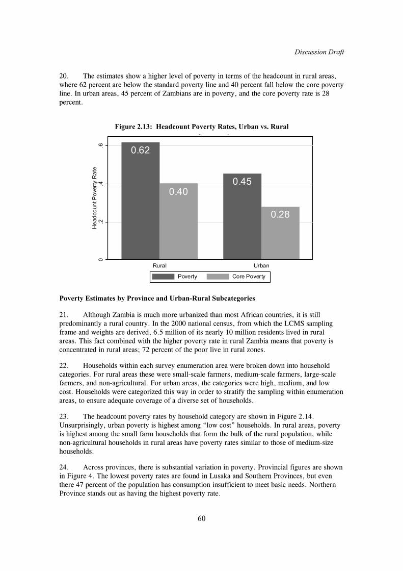
19. The national headcount estimates are 0.56 for poverty and 0.36 for core poverty. In
other words, over half of Zambians have levels of consumption that are insufficient to meet
basic needs, and more than a third have consumption levels that would be inadequate to meet
basic food needs alone, even if the individual were able to forego all non-food consumption.
Figure 2.13 shows poverty and core poverty rates for urban and rural households separately.
Due to weaknesses in the price data, it was not possible to satisfactorily adjust the consumption
data for urban-rural price differences. As a result comparisons in poverty figures across the
urban-rural divide do not reflect differences in the cost of living between urban and rural areas.
Poverty comparisons between rural and urban areas should therefore be treated with caution.
Discussion Draft
60
20. The estimates show a higher level of poverty in terms of the headcount in rural areas,
where 62 percent are below the standard poverty line and 40 percent fall below the core poverty
line. In urban areas, 45 percent of Zambians are in poverty, and the core poverty rate is 28
percent.
Figure 2.13: Headcount Poverty Rates, Urban vs. Rural
0.62
0.400.45
0.28
0.2
.4.6
He
ad
co
un
t P
overt
y R
ate
Rural Urban
y ,
Poverty Core Poverty
Poverty Estimates by Province and Urban-Rural Subcategories
21. Although Zambia is much more urbanized than most African countries, it is still
predominantly a rural country. In the 2000 national census, from which the LCMS sampling
frame and weights are derived, 6.5 million of its nearly 10 million residents lived in rural
areas. This fact combined with the higher poverty rate in rural Zambia means that poverty is
concentrated in rural areas; 72 percent of the poor live in rural zones.
22. Households within each survey enumeration area were broken down into household
categories. For rural areas these were small-scale farmers, medium-scale farmers, large-scale
farmers, and non-agricultural. For urban areas, the categories were high, medium, and low
cost. Households were categorized this way in order to stratify the sampling within enumeration
areas, to ensure adequate coverage of a diverse set of households.
23. The headcount poverty rates by household category are shown in Figure 2.14.
Unsurprisingly, urban poverty is highest among “low cost” households. In rural areas, poverty
is highest among the small farm households that form the bulk of the rural population, while
non-agricultural households in rural areas have poverty rates similar to those of medium-size
households.
24. Across provinces, there is substantial variation in poverty. Provincial figures are shown
in Figure 4. The lowest poverty rates are found in Lusaka and Southern Provinces, but even
there 47 percent of the population has consumption insufficient to meet basic needs. Northern
Province stands out as having the highest poverty rate.

Discussion Draft
61
Figure 2.14: Headcount Poverty Rates by Urban-Rural Subcategories
0.63
0.41
0.47
0.24
0.30
0.13
0.46
0.34
0.53
0.33
0.28
0.13 0.12
0.06
0.2
.4.6
He
ad
co
un
t P
ove
rty R
ate
Small_fa
rm
Med
_far
m
Larg
e_fa
rm
Rur
al_n
onag
Urb
an_low
_cos
t
Urb
an_m
ed_c
ost
Urb
an_h
igh_
cost
y y g
Poverty Core Poverty
Figure 2.15: Headcount Poverty Rates by Province
0.5
40
.32
0.5
20
.35
0.5
60
.34
0.6
7
0.4
7
0.4
7
0.2
9
0.7
50
.54 0.6
10
.37 0
.47
0.2
5
0.5
20
.35
0.2
.4.6
.8H
ead
co
un
t P
overt
y R
ate
Cent
ral
Copp
erbelt
Eas
tern
Luapu
la
Lusaka
North
ern
North
wes
tern
Sou
thern
West
ern
y y
Poverty Core Poverty
25. Table 2.10 shows separate headcount rates by urban and rural areas within each
province, and Table 2.11 displays a corresponding breakdown of where the poor are located.
The urban poor are highly concentrated in just two provinces, Lusaka and Copperbelt. The
urban areas of just those two provinces are home to 20 percent of Zambia’s poor, while the
smaller urban areas of the remaining provinces account for only an additional eight percent.

Discussion Draft
62
The rural poor are more widely distributed. They are most concentrated in Eastern and
Northern Provinces, the rural areas of which are home to 28 percent of the nation’s poor.
Table 2.10 Headcount Poverty Estimates by Province and
Urban/Rural
Rural Std. Err. Urban Std. Err.
Central 0.55 0.04 0.52 0.07
Copperbelt 0.65 0.05 0.48 0.04
Eastern 0.58 0.03 0.34 0.09
Luapula 0.70 0.04 0.48 0.08
Lusaka 0.63 0.08 0.43 0.04
Northern 0.78 0.03 0.59 0.07
Northwestern 0.64 0.03 0.37 0.08
Southern 0.51 0.03 0.32 0.05
Western 0.53 0.04 0.40 0.08
Table 2.11 Where Are the Poor? Fraction of National Poor by Province and
Urban/Rural
Province
Fraction of
National Poor
Living in
Province
Fraction of National
Poor Living in
Province's Rural
Areas
Fraction of National
Poor Living in
Province's Urban
Areas
Central 0.10 0.08 0.02
Copperbelt 0.15 0.04 0.11
Eastern 0.13 0.13 0.01
Luapula 0.09 0.08 0.01
Lusaka 0.12 0.03 0.09
Northern 0.17 0.15 0.02
Northwestern 0.06 0.06 0.01
Southern 0.10 0.09 0.02
Western 0.07 0.06 0.01
Total 1.00 0.72 0.28
Differences in Methodology with Central Statistical Office
26. The methodology employed in this paper is broadly similar to that used by the Zambia
CSO in its own analysis of the 2002-03 LCMS data. However, the methodology differs in
several key details:
Reference prices: Median prices vs. Lusaka cycle 1 prices
27. As the reference prices for its price index, CSO used prices collected in Lusaka
Province during the first of ten cycles, where a cycle corresponds to a data collection period
lasting 36 days. The danger in using such a narrow set of prices is that the results will be

Discussion Draft
63
sensitive to outliers in the data. The LCMS price data, like much price data from developing
countries, is extremely noisy, with implausibly large variation in prices across time and space.
28. As Deaton and Zaidi (2002) note, “A good choice [for reference prices] is to take the
median of the prices observed ….” They argue that the use of medians reduces sensitivity to
outliers. Furthermore, “[t]he use of a national average price vector ensures that the money
metric measures conform as closely as possible to national income accounting practice, as well
as eliminating results that might depend on a price relative that occurs only rarely or in some
particular area.”
29. An additional reason to favor the use of median prices is that for future comparisons
over time with new data, it will be necessary to replicate the price concept underlying the 2002-
03 poverty estimates. Because the timing and design of a future survey may differ somewhat, it
may not be possible to collect prices that correspond well to the Lusaka cycle 1 prices in the
2002-03 survey. For these reasons, the analysis in this paper use a price index referenced to
national median prices.
Price index: Single-stage vs. two-stage
30. CSO employed a two-stage price index procedure rather than a single-stage index.
First, consumption figures were adjusted over time, to cycle 1 within each province, using a
province-specific temporal price index. Second, the consumption data was adjusted to Lusaka
cycle 1 using a second spatial price index.
31. In the judgment of this author, the two-stage index unnecessarily doubles the number of
calculations and involves the province-specific cycle 1 price data, which introduces new error
into the calculations. The use of a single-stage price index, adjusting consumption directly from
a province-cycle set of prices to national median prices, reduces the number of calculations and
bypasses the province cycle 1 data. As explained above, this single-stage price index can be
used to produce summary price indices at the province and cycle levels.
Price index: Adjust non-food and durable goods components?
32. Like most developing country household consumption surveys, the LCMS includes
price data for food but not non-food goods. The familiar question arises as to what price
adjustment, if any, to apply to the non-food portion of consumption. Both for this paper and for
the CSO analysis, a composite price index was constructed based on the food price index and a
housing price index was constructed using the coefficients from the housing cost imputation.
What price adjustment should be applied to the remaining non-food components, which are the
durable goods user fee and other non-food? CSO applied the food price index to these
components. This is sensible, assuming that food and non-food prices tend to be correlated.
However, it is not clear that they are correlated, and they may even be negatively correlated if,
for example, transport costs are important so that in rural areas agricultural goods are cheaper
and manufactured goods are more expensive. Given this uncertainty, for this paper the
remaining non-food components are left in nominal terms.
Calorie requirement used to calculate poverty line
33. CSO reports that it has used a calorie requirement of 2094 calories per capita, although
it calculated its poverty figures on a per adult equivalent basis. CSO employed the same adult

Discussion Draft
64
equivalents used in an earlier study, Republic of Zambia (1997), based on calorie requirements
established by the National Food and Nutrition Commission (1993).31
34. The analysis in this paper uses calorie requirements based on World Health
Organization guidelines. The WHO figures were chosen so as to give the poverty line as solid a
basis as possible in a widely recognized reference.
Determination of food basket underlying poverty line
35. In general, quantity data by food item is required to construct a food basket for a food
poverty line. Because the 2002-03 LCMS did not include direct quantity data, it was necessary
to use some sort of second best procedure.
36. CSO chose to calculate average item shares in expenditure for a group of households
with expenditure per adult equivalent equal to the unweighted median plus or minus 20 percent.
Next, representative expenditures by item were calculated by multiplying these shares by
median expenditure. These expenditure values were then divided by Lusaka cycle 1 prices to
generate quantities for a preliminary consumption basket.
37. Given the data imperfections, the first part of the CSO procedure is reasonable. The
households in a range around the median provide a plausible set of nationally representative
expenditure shares by item. However, because these expenditure shares are for the country as a
whole, to convert these shares to quantities, some set of nationally representative prices should
be used, rather than Lusaka cycle 1 prices. The obvious choice would be national median
prices.
38. Calculating quantities by dividing national average expenditure shares by Lusaka cycle
1 prices is inconsistent and distorts the composition of the food basket. The resulting basket is
representative neither of the nation as a whole nor of Lusaka during cycle 1. Relative to a truly
nationally representative food basket, CSO’s resulting food basket has too little of foods that are
expensive in Lusaka cycle 1 and too much of those that are cheap in Lusaka cycle 1.
39. For purposes of this paper, a different procedure was used to determine the food
basket. Quantities were estimated at the household-item level by dividing reported expenditures
by province-cycle prices. Because the price data is noisy and does not reflect the actual prices
paid by individual households, this procedure is inferior to the use of true quantity data.
Nonetheless, it is the best approximation available to household-level quantities. Next, average
quantities were calculated for households in the middle (3rd) quintile nationally. These items
were ranked in descending order by cost for the average quantity, at national median prices.
The final food basket was defined as the top 44 items, which accounts for 90% of the cost of
the preliminary basket.
40. Using the list of items produced by its method, CSO chose to use the top 61 food items,
accounting for 94% of expenditure in the preliminary list. This cutoff (and the 90% cutoff used
for this paper) is arbitrary.
31 The adult equivalent weights are 0.36 for a child aged less than 4, 0.62 for age 4-6, 0.78 for age 7-9, 0.95 age 10-12, and 1.0 for all others.

Discussion Draft
65
41. Separate from the question of how to determine the quantities in the food basket is the
issue of the choice of prices used to cost the food basket when determining the poverty line.
The price index is used to adjust nominal consumption values, and the adjusted consumption
values are used to determine poverty rates. It follows that the food basket must be priced using
the same set of prices which are the reference prices for the price index. Accordingly, CSO
priced its basket using Lusaka cycle 1 prices, while for this paper the basket was priced with
national median prices.