2 (mth5113) lecture notes
TRANSCRIPT
MTH5113: INTRODUCTION TO DIFFERENTIAL GEOMETRYLECTURE NOTES (2020–2021)
DR. ARICK SHAO
1. Introduction to Curves and Surfaces
In this module, we will study geometry. According to our favourite source Wikipedia[11], geometry is the branch of mathematics that deals with the shapes and sizes ofobjects. Throughout this term, you will develop a better understanding of theseconcepts, as well as explore how they can be quantified and computed.
In your mathematical education—for instance, in calculus and linear algebra—youhave considered flat, linear spaces such as the real line (R), the Euclidean plane (R2),and higher-dimensional Euclidean spaces (Rn). This module will expand your outlookto curved settings. For example, how is the study of the surface of a ball similar to,and different from, the study of a flat piece of paper?
Another aim of this module, as suggested by its title, is to apply ideas and toolsfrom calculus and linear algebra to study these geometric questions. In addition,we will use the geometric insights we gain to obtain new understandings of familiarconcepts, such as vectors, differentiation, and integration.
1.1. Frequently Asked Questions. Before launching into more serious discussions,let us first address some common questions you may have regarding this module.
Question 1.1. Why would I want to study curved objects?
Curved objects can be found everywhere in our lives:
• If you throw a ball or shoot a rocket into the air, then the trajectory of theball or rocket will be curved rather than linear. Curves have also historicallybeen used in astronomy to model the motions of celestial bodies.
• The surface of the earth is not flat, but like a sphere. To study this surfaceas a whole, we have to understand the effects of its curvature. Historically,this has played important roles in navigation and astronomy; a very concreteexample is determining the shortest flight path between two cities.
1

2 (MTH5113) LECTURE NOTES
• According to Einstein’s landmark theory of general relativity, the universethat we inhabit is not flat, but rather a 4-dimensional curved object (called a“spacetime”). Moreover, gravity itself is modelled by the shape and curvatureof this spacetime. In fact, a careful understanding of this curvature is necessaryfor the GPS systems in our phones to work correctly!
These are only a few motivations for having a firmer understanding of geometry.As this is an introductory module, we will unfortunately have to restrict our discus-
sions here to one-dimensional (curves) and two-dimensional (surfaces) objects. If youare interested in four-dimensional spacetimes and gravity, then you should considerthe third-year module MTH6132: Relativity.
Question 1.2. Sounds interesting. But, what maths will I need to know?
This module is mainly concerned with the differential geometry of curves and sur-faces. In particular, we look at objects that “vary smoothly enough” so that wecan take derivatives, or linear approximations, of them. Moreover, to measure thesizes—e.g. length and area—of objects, we will need to compute various integrals.
As a result, this module will assume you have moderate familiarity with first-yearcalculus, for which differentiation and integration are two cornerstones.
• In our study of curves, we will make frequent use of single-variable calculus(mainly, contents from MTH4*00: Calculus I).
• For surfaces, we will require knowledge of partial derivatives and double/tripleintegrals (which you saw in MTH4*01: Calculus II).
The simplest geometric objects that we can consider are lines and planes; these fallunder the study of linear algebra. For this task, we will sometimes refer to backgroundknowledge in MTH4*15: Vectors and Matrices, as well as either MTH5112: LinearAlgebra I or MTH5212: Applied Linear Algebra.
Even for more complex curved objects, a useful tool in their analysis is linearisa-tion—to first study the linear objects that best approximate them. Thus, we cannotreally escape the need to understand linear algebra and its connections to geometry.
Finally, in order to construct a diverse collection of examples of geometric objects,we will make use of many elementary functions:
• Polynomials (e.g. t2 + 1), and rational functions (quotients of polynomials).• Trigonometric (sin, cos) and hyperbolic (sinh, cosh) functions.
(MTH5113) LECTURE NOTES 3
• Exponential (exp) and logarithmic (ln) functions.We will, at times, reference a few basic properties of these functions.
If you want to be optimally prepared for this module, then it is recommended thatyou revise the material you learned in calculus and linear algebra.
Question 1.3. Help! What will I be expected to do?
The main focus of the module is on the interface between some mathematics youhave already seen—most notably, calculus and linear algebra—and concepts in geom-etry. For example, you will be expected to understand how notions such as deriva-tives, integrals, vectors, and matrices connect with studying the shapes and sizes ofobjects. This is primarily conceptual and is more about understanding the materialin a critical way rather than memorising definitions and formulas.
As the module is also concerned with quantifying geometric properties, you will beexpected to demonstrate that you are capable of performing various types of compu-tations. Again, these computations will involve elements of calculus (e.g. derivativesand integrals) and linear algebra (e.g. vector computations).
You should also gain a visual understanding of these geometric concepts. As aresult, you will be asked to graph various curves and surfaces, on a plane or in space.
Finally, though we will encounter a number of proofs in our discussions, they willnot be a central focus of this module. In particular, you will not be asked to memoriseand recite lengthy proofs of various results that you will encounter. On the other hand,you will need to have a general understanding of why results are true.
Question 1.4. I can do it! Now, what will I actually learn in the module?
In the remainder of this chapter, we give a brief and informal outline of the mainthemes to be discussed throughout this module.
1.2. Vectors and Calculus, Revisited. The first part of the module is gearedtoward revising various aspects of vector algebra and calculus. This provides anopportunity for you to revisit details that you have forgotten and to fill in gaps inyour existing knowledge. However, rather than simply repeating material you havealready learned (boring!), we will also introduce new geometric perspectives, therebydeveloping a different and more refined understanding of old ideas.
The module begins by revisiting the notion of vectors and their role in geometry.As you know well, vectors are often visually depicted as arrows. We will develop this

4 (MTH5113) LECTURE NOTES
simple intuition formally, via the notion of tangent vectors. Later, these objects willplay key roles in quantifying various geometric properties of curves and surfaces.
From here, we move into the study of vector-valued functions and vector fields (seeFigure 1.1). These are used to represent a variety of physical phenomena, such as fluidflow, gravitational fields, and the populations of competing species in an ecosystem.Our objective is to better understand how such quantities are depicted visually, as wellas to remind ourselves of how to perform various computations with these objects.
Figure 1.1. The two graphics depict vector fields on a plane. The leftvector field describes clockwise rotation around the origin, while the rightvector field describes attraction toward the origin.
The main focus of this discussion will be on calculus. First, we recall the standarddifferential operations in vector calculus (e.g. derivatives and partial derivatives). Weextend these concepts to vector-valued functions, and we revise how these derivativescan be computed. We then turn our attention toward the other side of calculus—integration. In particular, we discuss the view of integrals as “weighted” lengths,areas, and volumes; we then recall some basic tricks for computing them.
1.3. The Geometry of Curves. With revisions behind us, we next move into thecore of the module: studying the geometry of curves and surfaces. The first half ofthis effort focuses on 1-dimensional geometric objects: curves.
The first step is to make precise sense of what a curve is, by formulating a rigorousdefinition of curves. We then discuss some familiar ways to describe curves, forinstance, parametrically or as level sets of functions. One fundamental idea hereis independence of parametrisation—although one can view a curve from differentperspectives, all these viewpoints are of the same underlying object.
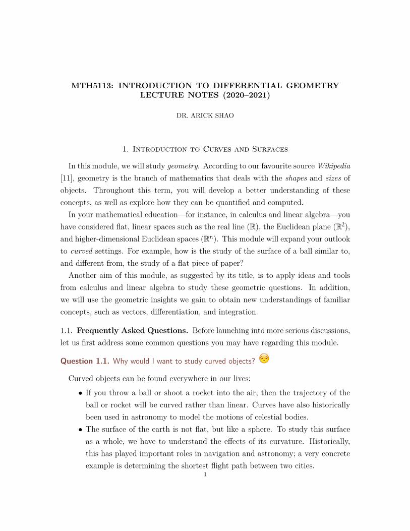
We will also explore various geometric properties of curves. As a basic example,consider the curves C1, C2, C3 in Figure 1.2. Your intuition likely tells you C1 is
(MTH5113) LECTURE NOTES 5
“straight”, while C2 and C3 are “curved”. You probably also sense C3 is “more curved”than C2. But, how might you capture and quantify this mathematically?
x
yC1
C2
C3
x
yT1T2
Figure 1.2. In the left graphic, C1 is “straight” while C2 and C3 are“curved”. On the right, T1 and T2 are circles with different circumferences.
Another aspect of geometry is studying the sizes of objects. Consider the circles T1and T2 in Figure 1.2. Intuitively, T1 and T2 have similar shapes but different “sizes”.You probably also have enough background to know that this can be captured bymeasuring their arc lengths (i.e. circumferences).
From calculus, you know that lengths are generally evaluated using integrals, andyou should be familiar with integrals along an interval of the real line. The questionof computing arc lengths will force us to make sense of what it means to integrateinstead along curves, leading us to the notion of curve or path integrals. As we will see,curve integrals are a powerful abstraction with a variety of applications; one examplefrom classical mechanics is the total work done by a force.
1.4. The Geometry of Surfaces. The other half of our foundations concerns thegeometry of surfaces. This is largely analogous to the study of curves, but now theobjects are 2-dimensional, which brings forth a new batch of complications.
Again, our analysis begins with precisely defining what a surface is, as well as withdevising various methods for describing surfaces (e.g. parametrically or as level setsof functions). We then move on to study various geometric properties of surfaces.
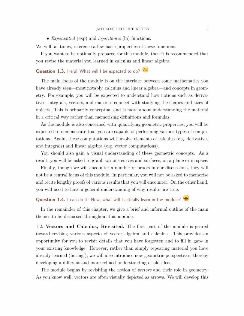
Considering the surfaces in Figure 1.3, you can distinguish that S1 is “flat”, whileS2, S3, and S4 are “curved”. You can also tell when a surface is “very curved” asopposed to “slightly curved” (for instance, S3 and S2). What is novel, in contrast tocurves, is that a surface can bend in different ways along different directions. For
6 (MTH5113) LECTURE NOTES
instance, both spheres S2 and S3 always bend inward toward itself, while the “saddle”S4 bends both toward and away from itself, depending on which direction you look.
x
yz S1
x
y
z S2
x
y
z S3
x
y
z S4
Figure 1.3. S1, S2, S3, S4 are surfaces in 3-dimensional space. S1 is “flat”,while the remaining surfaces are “curved”.
Yet another interesting example of a geometric property of surfaces is orientability—whether a surface is “two-sided”. Most familiar examples, including all the surfacesfound in Figure 1.3, are two-sided. However, we will also encounter some exoticsurfaces that are not two-sided, such as the Möbius strip and the Klein bottle.
We will also discuss how one measures the size—that is, the area—of a surface. Forinstance, the spheres S2 and S3 in Figure 1.3 have similar shapes but different sizes.In analogy with previous discussions for curves, this leads us to an integration theoryalong surfaces. Again, these surface integrals can used to model many phenoma; aclassical example from physics is the electric flux through a surface.
1.5. Putting It All Together. In later parts of this module, we will gather all thetheory we have developed—a hybrid of geometry, calculus, and linear algebra—andexplore some topics and problems lying at the intersection of all these areas.
A classical problem in calculus that you have already encountered is that of findingthe maximum and minimum values of a function, as well as where these values areattained. Here, we see how this analysis generalises to functions defined on curvesand surfaces. For instance, can we use similar strategies to find, say, the locations onthe earth’s surface having the highest temperature?
(MTH5113) LECTURE NOTES 7
Moreover, we will attack this same problem from a different viewpoint—we rebrandit as a problem of optimising a function (on the larger space) subject to contraints (i.e.we only care about the points lying on a curve or surface). This leads to the methodof Lagrange multipliers, which has widespread applications in physics, engineering,and economics, as well as within mathematics itself.
We will conclude the module with some landmark theorems from vector calculus.A starting point of this discussion is the famous fundamental theorem of calculus,
(1.1)∫b
a
f ′(t)dt = f(b) − f(a),
which highlights a deep, and in many ways incredible, connection between differ-entiation and integration. We can then ask whether there are higher-dimensional,geometric generalisations of the fundamental theorem of calculus.
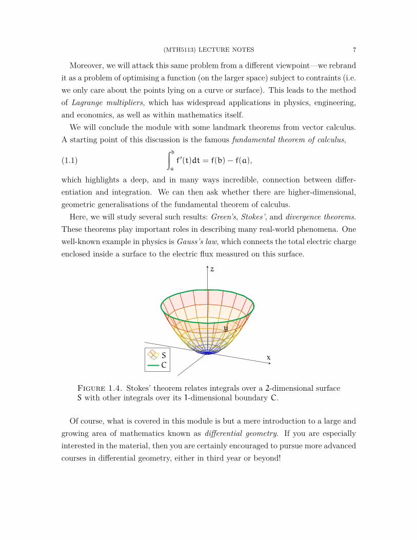
Here, we will study several such results: Green’s, Stokes’, and divergence theorems.These theorems play important roles in describing many real-world phenomena. Onewell-known example in physics is Gauss’s law, which connects the total electric chargeenclosed inside a surface to the electric flux measured on this surface.
x
y
z
S
C
Figure 1.4. Stokes’ theorem relates integrals over a 2-dimensional surfaceS with other integrals over its 1-dimensional boundary C.
Of course, what is covered in this module is but a mere introduction to a large andgrowing area of mathematics known as differential geometry. If you are especiallyinterested in the material, then you are certainly encouraged to pursue more advancedcourses in differential geometry, either in third year or beyond!
8 (MTH5113) LECTURE NOTES
2. Vector Calculus
In this chapter, we revisit a number of concepts from vector algebra and vectorcalculus that you have seen before. This will include a sample of contents from:
• MTH4*00: Calculus I• MTH4*01: Calculus II• MTH4*15: Vectors and Matrices• MTH5*12: Linear Algebra I/Applied Linear Algebra
One objective of this chapter is to refamiliarise yourself with content from thesemodules, as we will make ample use of them later in these notes.
In addition, we will approach these topics from a different, and more geometric,point of view. Thus, while all of this material should already be rather familiar toyou, we will nonetheless aim to build a different understanding of it.
2.1. Tangent Vectors. We begin this discussion with some very basic stuff: vectors.When you first learned of vectors, you were likely taught to visualise them as “arrows”lying in a plane or in space. More specifically, you probably viewed these arrows as“starting from a point” and “pointing in some direction”.
On the other hand, for algebraic purposes, one had a different outlook:
Definition 2.1. Let Rn denote the n-dimensional Euclidean space,
(2.1) Rn = {(x1, x2, . . . , xn) | x1, x2, . . . , xn ∈ R},
consisting of all n-tuples of real numbers.
In linear algebra, you saw vectors as elements of the set Rn (or, more abstractly,as elements of a vector space). For example, a 2-dimensional vector would be a pairv = (v1, v2) of real numbers, while a 3-dimensional vector would likewise be a triplew = (w1, w2, w3). You could then proceed to define several algebraic operations,such as vector addition and scalar multiplication, on Rn.
Remark 2.2. In practice, the module will only involve 1, 2, and 3-dimensional settings.However, it is often not any more difficult to work in all dimensions.
While Rn is convenient for algebraic computations, the perspective of treatingvectors as arrows contains a number of geometric intuitions that will prove useful.Therefore, we now develop this idea in a more formal manner.
To describe such an arrow, say in Rn, we require two pieces of information:
(MTH5113) LECTURE NOTES 9
• The starting point p ∈ Rn of the arrow.• The vector component v ∈ Rn of the arrow, representing both the direction in
which the arrow is pointing and the length of the arrow.From this, we can craft a mathematical object “vp” representing an arrow beginningat p and pointing along v; see the first drawing in Figure 2.1. For reasons that willbecome apparent later, we refer to these arrows as tangent vectors:
Definition 2.3. A tangent vector in Rn is a pair vp, with v,p ∈ Rn, which formallyrepresents the “arrow” in Rn starting at the point p and having pointing along v.
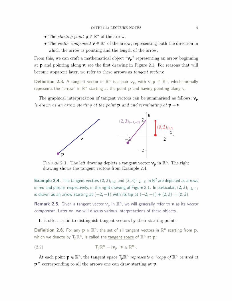
The graphical interpretation of tangent vectors can be summarised as follows: vp
is drawn as an arrow starting at the point p and and terminating at p+ v.
p
v −2 2
−2
2
(0, 2)(1,0)
(2, 3)(−1,−2)
x
y
Figure 2.1. The left drawing depicts a tangent vector vp in Rn. The rightdrawing shows the tangent vectors from Example 2.4.
Example 2.4. The tangent vectors (0, 2)(1,0) and (2, 3)(−2,−1) in R2 are depicted as arrowsin red and purple, respectively, in the right drawing of Figure 2.1. In particular, (2, 3)(−2,−1)
is drawn as an arrow starting at (−2,−1) with its tip at (−2,−1) + (2, 3) = (0, 2).
Remark 2.5. Given a tangent vector vp in Rn, we will generally refer to v as its vectorcomponent. Later on, we will discuss various interpretations of these objects.
It is often useful to distinguish tangent vectors by their starting points:
Definition 2.6. For any p ∈ Rn, the set of all tangent vectors in Rn starting from p,which we denote by TpRn, is called the tangent space of Rn at p:
(2.2) TpRn = {vp | v ∈ Rn}.
At each point p ∈ Rn, the tangent space TpRn represents a “copy of Rn centred atp”, corresponding to all the arrows one can draw starting at p.

10 (MTH5113) LECTURE NOTES
Having gone through the trouble of formally defining tangent vectors, we shouldnow ask what we can do with them that would be geometrically meaningful. Let usbegin here with the most basic vector operations from linear algebra:
Definition 2.7. Let p ∈ Rn. We define the following operations on tangent vectors:• Given tangent vectors vp,wp ∈ TpRn, both starting from p, we define
(2.3) vp +wp = (v+w)p.
• Given a tangent vector vp ∈ TpRn and a scalar c ∈ R, we define
(2.4) c · vp = (c · v)p.
Both operations in Definition 2.7 have natural geometric interpretations—in fact,the same ones you have seen since you first learned about vectors. These are demon-strated in the two pictures in Figure 2.2, both of which you should find quite familiar.In particular, the right graphic in Figure 2.2 is the standard parallelogram diagramthat is commonly used to describe vector addition.
p vp
2 · vp
p
vpwp
vp +wp
Figure 2.2. The left graphic demonstrates the geometric meaning of (2.4),while the right graphic shows the geometric meaning of (2.3).
Example 2.8. Addition and scalar multiplication of tangent vectors are very simple, sinceone just applies the usual operations to the vector components. The following exampleuses (2.3) to add two tangent vectors in R2, both starting from (−1, 0):
(1, 2)(−1,0) + (3,−1)(−1,0) = [(1, 2) + (3,−1)](−1,0)
= (4, 1)(−1,0),
Similarly, the following applies (2.4) to a tangent vector in R3:
−2 · (1, 2, 3)(−1,−2,−3) = [−2 · (1, 2, 3)](−1,−2,−3)
= (−2,−4,−6)(−1,−2,−3).

(MTH5113) LECTURE NOTES 11
On the other hand, according to Definition 2.7, the sum
(0, 1)(0,0) + (1, 0)(0,1)
is not defined, since the two tangent vectors are based at different points!
Returning now to the language of linear algebra, one can verify (you should try ityourself!) that TpRn and the two operations in Definition 2.7 satisfy all the axioms ofa vector space. Thus, the tangent spaces TpRn are concrete examples of the abstractvector spaces that you studied in linear algebra.
Definition 2.9. Given v = (v1, . . . , vn) ∈ Rn, we define its norm by
|v| =√
v21 + v22 + · · ·+ v2n.
Moreover, for a tangent vector vp ∈ TpRn, we define its norm to be
(2.5) |vp| = |v|.
In particular, the norm of a tangent vector is just the norm of its vector component.The geometric interpretation of this should be familiar to you:
• The norm |vp| captures the length of the arrow vp.• When |vp| 6= 0, the unit tangent vector pointing in the same direction as vp is
1
|vp|· vp.
Example 2.10. The norm of the tangent vector (1, 2,−1, 7)(0,0,0,0) in R4 is
|(1, 2,−1, 7)(0,0,0,0)| = |(1, 2,−1, 7)|
=√55.
2.2. Dot and Cross Products. We now recall a very familiar vector operation—thedot product—and we extend it to tangent vectors.
Definition 2.11. Given two n-dimensional vectors,
v = (v1, . . . , vn) ∈ Rn, w = (w1, . . . , wn) ∈ Rn,
we define their dot product by
(2.6) v ·w = v1w1 + v2w2 + · · ·+ vnwn ∈ R.

12 (MTH5113) LECTURE NOTES
Also, for tangent vectors vp and wp in Rn, both starting at p ∈ Rn, we define
(2.7) vp ·wp = v ·w.
In particular, (2.6) is the usual formula that you have seen for years. For tangentvectors, their dot product is simply the dot product of their vector components.
Remark 2.12. Note that while v and w are vectors, their dot product v ·w is a scalar,not a vector. A similar statement holds for tangent vectors.
Example 2.13. An example of a dot product of tangent vectors in R2 is given below:
(1, 2)(−1,−1) · (−1, 2)(−1,−1) = (1, 2) · (−1, 2)
= 1 · (−1) + 2 · 2
= 3.
On the other hand, according to Definition 2.11, the dot product
(1, 2)(−1,−1) · (−1, 2)(−1,0)
is not defined, since the two tangent vectors are based at different points.
While (2.6) and (2.7) are most convenient for computations, another formula fordot products has more illuminating geometric interpretations:
Theorem 2.14. For v,w,p as in Definition 2.11, we have
(2.8) vp ·wp = |vp||wp| cos θ,
where θ is the angle made between the arrows vp and wp at p. In particular,
(2.9) |vp|2 = vp · vp.
The formula (2.8) indicates that dot products carry two pieces of information:• The lengths of the tangent vectors involved.• The angle between the tangent vectors involved.
In the case of (2.9), as there is only one vector involved (hence θ vanishes), the dotproduct vp · vp carries information only about the length of vp.
Figure 2.3 gives the standard illustration of (2.8). Note that the use of tangentvectors formally realises this drawing, since the angle θ is now manifested as the anglemade between two arrows at their common starting point p.

(MTH5113) LECTURE NOTES 13
p
vw
θ
Figure 2.3. This drawing demonstrates the setting of (2.8).
Next, we embark on a similar discussion for cross products:
Definition 2.15. Given two 3-dimensional vectors
v = (v1, v2, v3) ∈ R3, w = (w1, w2, w3) ∈ R3,
we define their cross product to be the 3-dimensional vector
(2.10) v×w = (v2w3 − v3w2, v3w1 − v1w3, v1w2 − v2w1) ∈ R3.
Moreover, for two tangent vectors vp,wp ∈ TpR3, we define
(2.11) vp ×wp = (v×w)p.
Remark 2.16. An easy way to remember (2.10) is to express it informally as
(2.12) v×w = det
i j k
v1 v2 v3
w1 w2 v3
,
where i, j, k denote the canonical basis for R3:
i = (1, 0, 0), j = (0, 1, 0), k = (0, 0, 1).
Remark 2.17. Keep in mind that the cross product v × w of 3-dimensional vectors isitself a 3-dimensional vector, not a scalar. Similarly, the cross product of two tangentvectors in R3 is itself a tangent vector in R3, based at the same point.
Also, remember that cross products are specific to 3 dimensions. In particular, (please)never try to take cross products of 2-dimensional vectors!
To see why cross products are useful, we recall the following property:
Theorem 2.18. Let v,w,p be as in Definition 2.15.• If vp and wp point in the same or the opposite directions, then vp ×wp = 0.
14 (MTH5113) LECTURE NOTES
• Otherwise, vp ×wp points in the direction that is perpendicular to both vp andwp and satisfies the right-hand rule. Furthermore,
(2.13) |vp ×wp| = |vp||wp| sin θ,
where θ is the angle made between the tangent vectors vp and wp at p.
In particular, suppose you already have two vectors that span two of the three di-mensions in R3. Then, their cross product provides a straightforward and computableway to generate the remaining third dimension.
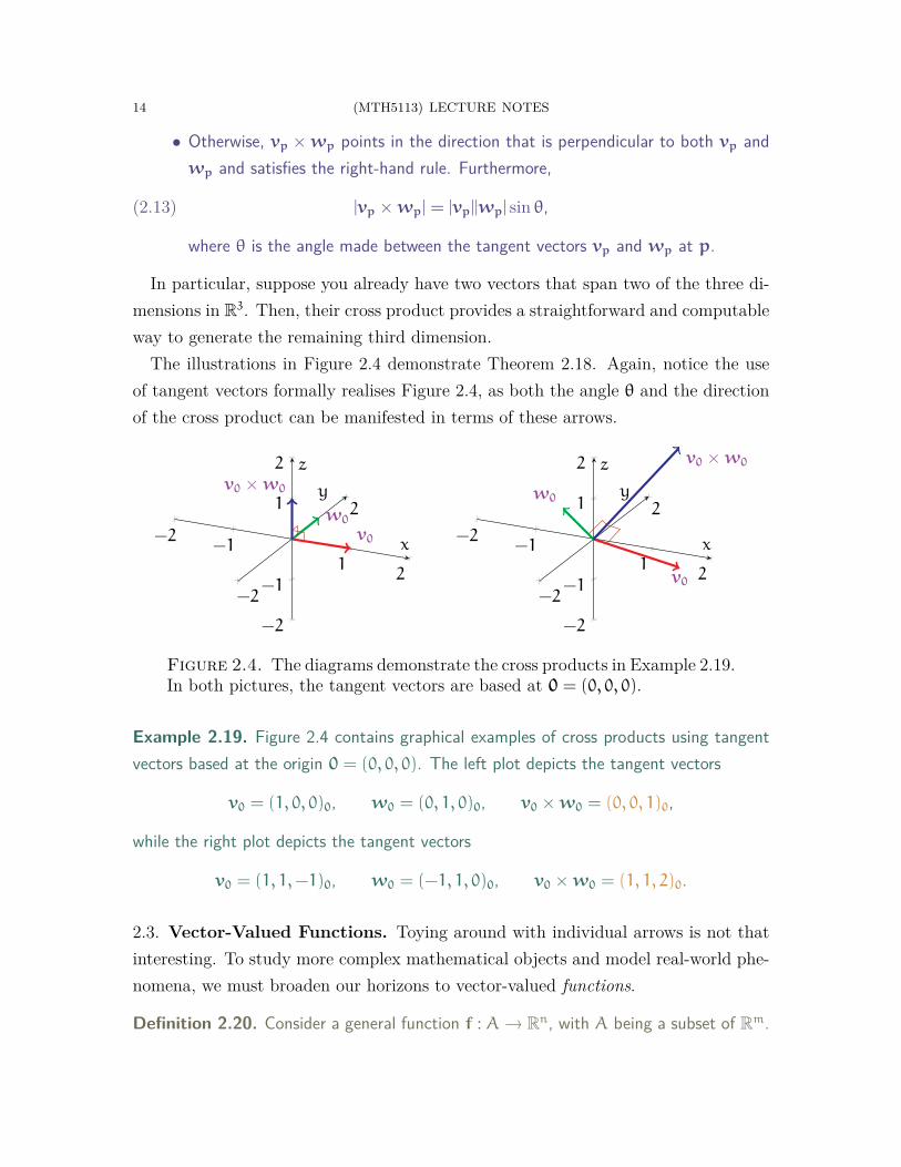
The illustrations in Figure 2.4 demonstrate Theorem 2.18. Again, notice the useof tangent vectors formally realises Figure 2.4, as both the angle θ and the directionof the cross product can be manifested in terms of these arrows.
−2−1
12
−2
2
−2
−1
1
2
v0
w0
v0 ×w0
x
y
z
−2−1
12
−2
2
−2
−1
1
2
v0
w0
v0 ×w0
x
y
z
Figure 2.4. The diagrams demonstrate the cross products in Example 2.19.In both pictures, the tangent vectors are based at 0 = (0, 0, 0).
Example 2.19. Figure 2.4 contains graphical examples of cross products using tangentvectors based at the origin 0 = (0, 0, 0). The left plot depicts the tangent vectors
v0 = (1, 0, 0)0, w0 = (0, 1, 0)0, v0 ×w0 = (0, 0, 1)0,
while the right plot depicts the tangent vectors
v0 = (1, 1,−1)0, w0 = (−1, 1, 0)0, v0 ×w0 = (1, 1, 2)0.
2.3. Vector-Valued Functions. Toying around with individual arrows is not thatinteresting. To study more complex mathematical objects and model real-world phe-nomena, we must broaden our horizons to vector-valued functions.
Definition 2.20. Consider a general function f : A → Rn, with A being a subset of Rm.
(MTH5113) LECTURE NOTES 15
• A is called the domain of f.• The image (or range) of f is the set of all possible values achieved by f:
f(A) = {f(x) | x ∈ A}.
Moreover, we can view this map f in a variety of equivalent ways:• We can think of f as mapping each vector x ∈ A to a vector f(x) ∈ Rn.• We could also view f as mapping each x ∈ A to n real values,
f(x) = (f1(x), f2(x), . . . , fn(x)) ∈ Rn.
In other words, f splits into n real-valued functions,
f = (f1, f2, . . . , fn), fk : A → R, 1 ≤ k ≤ n.
• Similarly, we can split a vector x ∈ A into its components, x = (x1, x2, . . . , xm),so that f can be viewed as a function of m real numbers:
f(x) = f(x1, . . . , xm) = (f1(x1, . . . , xm), . . . , fn(x1, . . . , xm)).
You should be at least somewhat familiar with the conventions in Definition 2.20from your previous experiences. In these notes, we will use both vector notations andexpanded components interchangeably, depending on context.
In the remainder of this section, we discuss a few concrete examples of vector-valuedfunctions. We begin with functions of one variable (m = 1):
0 1 2 3
x
R
−1 1
−1
1
x
y
γ
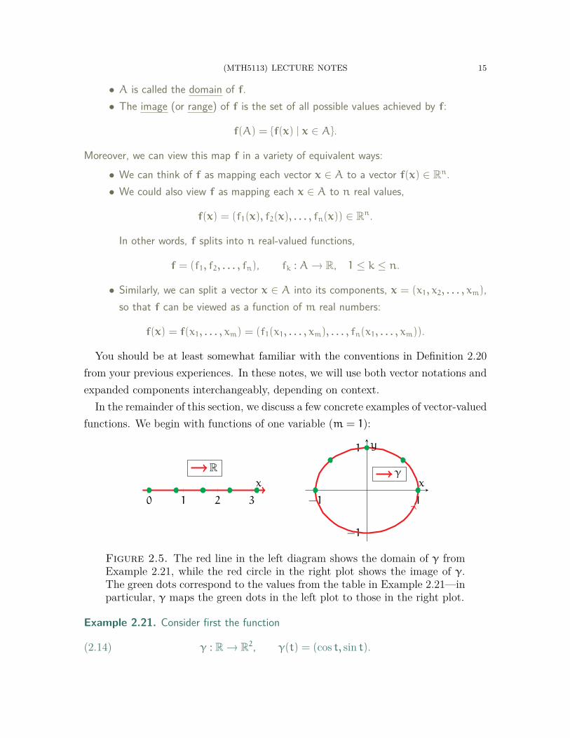
Figure 2.5. The red line in the left diagram shows the domain of γ fromExample 2.21, while the red circle in the right plot shows the image of γ.The green dots correspond to the values from the table in Example 2.21—inparticular, γ maps the green dots in the left plot to those in the right plot.
Example 2.21. Consider first the function
(2.14) γ : R → R2, γ(t) = (cos t, sin t).
16 (MTH5113) LECTURE NOTES
Note that γ maps any number t on the real line (i.e. the domain of γ, drawn in the leftpart of Figure 2.5) to the point (cos t, sin t) on the xy-plane.
To better understand the behaviour of γ, let us now plot its image. By default, such afunction can be plotted by hand using the following general procedure:
(1) The first step is to compute γ(t) for a “large enough” sample of points t. Somespecific values of γ are listed in the table below:
t 0 π4
π2
3π4
π
γ(t) (1, 0)(
1√2, 1√
2
)(0, 1)
(− 1√
2, 1√
2
)(−1, 0)
(2) Next, we plot the values γ(t) from step (1) onto the xy-plane. The green dotsin the left plot of Figure 2.5 show the values of t in the preceding table, while thegreen dots in the right plot represent the corresponding values for γ(t).
(3) Once you have enough values of γ plotted, you can then try to guess the imageof γ by “connecting the dots” in a reasonable manner.
By following the above steps, you should then be able to see that γ maps out the unitcircle about the origin; this is the red path in the right plot of Figure 2.5.
(All this could also be deduced from (2.14) itself, since cos t and sin t are the x andy-coordinates of the point on the unit circle whose angle from the positive x-axis is t.)
0 1 2 3
x
R
−2 −11
2−2
2
−2
2
x
y
z ℓ
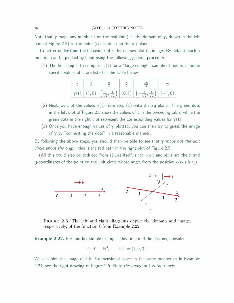
Figure 2.6. The left and right diagrams depict the domain and image,respectively, of the function ℓ from Example 2.22.
Example 2.22. For another simple example, this time in 3 dimensions, consider
ℓ : R → R3, ℓ(t) = (t, 0, 0).
We can plot the image of ℓ in 3-dimensional space in the same manner as in Example2.21; see the right drawing of Figure 2.6. Note the image of ℓ is the x-axis.
(MTH5113) LECTURE NOTES 17
In general, plotting single-variable functions onto a plane is rather straightforward,as one can follow the steps discussed in Example 2.21. Plotting functions in R3 isnot any harder in principle, though drawing a 3-dimensional picture on paper can betricky. Fortunately, you will not be asked to plot functions in 4 or more dimensions!
Finally, we turn our attention to vector-valued functions of multiple variables:
2 4 6
−1
1
u
v
−11
−1
1
−1
1
x
yz σ
−11
−1
1
−1
1
x
yz
−11
−1
1
−1
1
x
yz
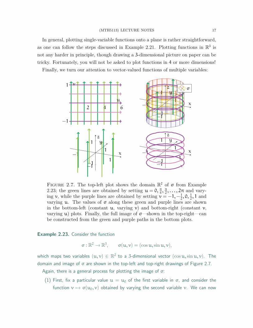
Figure 2.7. The top-left plot shows the domain R2 of σ from Example2.23; the green lines are obtained by setting u = 0, π
4, π2, . . . , 2π and vary-
ing v, while the purple lines are obtained by setting v = −1,− 12, 0, 1
2, 1 and
varying u. The values of σ along these green and purple lines are shownin the bottom-left (constant u, varying v) and bottom-right (constant v,varying u) plots. Finally, the full image of σ—shown in the top-right—canbe constructed from the green and purple paths in the bottom plots.
Example 2.23. Consider the function
σ : R2 → R3, σ(u, v) = (cosu, sinu, v),
which maps two variables (u, v) ∈ R2 to a 3-dimensional vector (cosu, sinu, v). Thedomain and image of σ are shown in the top-left and top-right drawings of Figure 2.7.
Again, there is a general process for plotting the image of σ:(1) First, fix a particular value u = u0 of the first variable in σ, and consider the
function v 7→ σ(u0, v) obtained by varying the second variable v. We can now

18 (MTH5113) LECTURE NOTES
plot this function in the same manner as in Examples 2.21 and 2.22. If we repeatthis for several values of u, then the resulting images—each of which is a path in3-dimensional space—will give us a good idea of what the image of σ looks like.This process is shown in the bottom-left plot in Figure 2.7.
(2) A complementary set of paths can be obtained from fixing values of v and varyingu instead. This is demonstrated in the bottom-right drawing in Figure 2.7.
(3) From the images obtained in steps (1) and (2), we can make a reasonable guessfor what the full image of σ looks like; see the top-right plot in Figure 2.7.
From the above, we conclude that the image of σ is a cylinder, centred about the z-axisand having radius 1. Observe that if we fix u and vary v, then we obtain a vertical lineof the cylinder, situated at a fixed polar angle. On the other hand, if we fix v and vary u,then we obtain a unit circle from the cylinder, situated at a fixed z-height.
Example 2.23 shows that plotting functions of two variables is also not so compli-cated in theory. However, the process can be more painstaking, since we may needto experiment by plotting several single-variable functions.
Remark 2.24. There is no need to panic if you are not comfortable with plotting functionsyet. We will explore many more examples in upcoming sections!
2.4. Limits and Continuity. Let us continue our discussions of vector-valued func-tions, except we now shift our focus toward some topological concepts.
In mathematics, topology refers to the study of properties preserved under continu-ous deformations. To visualise this, imagine bending a piece of wire without breakingit, or stretching a ball of clay without poking a hole in the middle. In doing this, youalter the shapes of the objects, but there are other attributes that stay unchanged.
Before addressing continuity, we must first recall a familiar idea from calculus:
Definition 2.25. Let the vector-valued fuction f : A → Rn be as in Definition 2.20, andlet p ∈ A. We say that L ∈ Rn is the limit of f at p, denoted
(2.15) limx→p
f(x) = L,
iff for every ε > 0, there exists some δ > 0 such that the following statement holds: ifx ∈ A, x 6= p, and |x− p| < δ, then |f(x) − L| < ε.
Definition 2.25 is, in essence, a statement about the behaviour of f near the pointp. Roughly, it says that f(x) gets as close as you want to L, as long as x is close
(MTH5113) LECTURE NOTES 19
enough to p. Moreover, the symbols “δ” and “ε” of calculus students’ nightmares canbe interpreted as follows: ε represents how close you want f(x) to be to L, while δ
represents how close x must be to p in order to achieve the desired ε-closeness.
Remark 2.26. One can still make sense of limits of f in Definition 2.25 at some pointsp 6∈ A. However, we will not need this extended definition here.
The following shows how limits of vector-valued functions can be computed:
Theorem 2.27. Let f = (f1, f2, . . . , fn) be as in Definition 2.20, and let p ∈ A. Then,
limx→p
f(x) = L,
where L = (L1, L2, . . . , Ln) ∈ Rn, if and only if for every 1 ≤ k ≤ n,
limx→p
fk(x) = Lk.
Proof. We avoid a formal proof here, as this would require some background fromMTH5104: Convergence and Continuity. However, the key idea is the identity
|f(x) − L|2 =
n∑k=1
|fk(x) − Lk|2.
From the above, one sees that f(x) becomes arbitrarily close to L if and only if fk(x)becomes arbitrarily close to Lk for each 1 ≤ k ≤ n. □
Theorem 2.27 implies that limits of vector-valued functions can be taken compo-nentwise. In other words, to compute the limit of a vector-valued function f, we needonly compute the limits of the individual real-valued components of f.
For completeness, we consider a simple example:
Example 2.28. Let us compute the limit, at t0 = −1, of the function
h : R → R3, h(t) = (t, t2, t3).
Applying Theorem 2.27, with f = h, we see that
limt→−1
h(t) =
(limt→−1
t, limt→−1
t2, limt→−1
t3)
= (−1, 1,−1),
where in the final step, the individual real-valued limits can be evaluated directly.
Next, we apply limits to define continuous functions:

20 (MTH5113) LECTURE NOTES
Definition 2.29. Let f be as in Definition 2.20. We say f is continuous at p ∈ A iff
(2.16) limx→p
f(x) = f(p).
In addition, we say f is continuous iff f is continuous at every p ∈ A.
In particular, (2.16) says that the values of f near the point p are close to f(p)
itself. In other words, the values of f do not “break”, or “jump”, while at p.
Example 2.30. The function from Example 2.21,
γ : R → R2, γ(t) = (cos t, sin t),
is continuous; see Figure 2.5 for plots of its domain and image.One can visualise this γ as taking an infinitely long wire (the left half of Figure 2.5) and
bending it into a circular shape (the right half of Figure 2.5). That this γ is continuouscan be seen from the fact that this bending does not break the wire at any point.Example 2.31. Another example of a continuous function is that of Example 2.23,
σ : R2 → R3, σ(u, v) = (cosu, sinu, v);
see Figure 2.7 for plots of the domain and image of σ.One can visualise σ as taking a piece of paper (the top-left drawing in Figure 2.7)
and rolling into up into a cylinder (the top-right drawing of Figure 2.7), though both thepaper and the cylinder have infinite dimensions here. Again, σ is continuous because this“rolling up” bends the paper but does not tear it at any point.
Figure 2.8. The above illustrates the function g from Example 2.32. Theleft and right drawings represent the domain and image of g, respectively.Notice that g fails to be continuous at the green point.
Example 2.32. For an example of something discontinuous, we consider the function g
roughly drawn in Figure 2.8. (The exact definition of g is not important here.)Here, g maps the lasso-shaped red path in the left half of Figure 2.8 (its domain) to
the path on the right half of this figure (its image). Moreover, the blue and green pointsin the domain are mapped to the blue and green points on the image, respectively.
(MTH5113) LECTURE NOTES 21
To see why g fails to be continuous, note that in the domain of g, the blue pointsconverge toward the green point p. On the other hand, the values of g at these bluepoints—that is, the blue points in the right drawing—do not tend to the green point g(p)in the right drawing. As a result, Definition 2.29 is violated at p.
Less formally, one can view the function g as bending the left drawing in Figure 2.8into the right drawing. However, to do this, one must also “cut” this left figure at thegreen point, hence making this deformation discontinuous.
Remark 2.33. We will not deal formally with limits and continuity in this module. How-ever, these will be of some importance in some later conceptual discussions.
2.5. Derivatives. The next step of our revisions is to discuss aspects of differentialcalculus, which is primarily concerned with studying how a function is changing. Inthis section, we begin with a very familiar concept:
Definition 2.34. Let I = (a, b) be an open interval, and let f : I → Rn be a vector-valuedfunction (of one variable). Then, the derivative of f at t0 ∈ I is defined to be
(2.17) f ′(t0) = limt→t0
f(t) − f(t0)
t− t0,
whenever the limit on the right-hand side of (2.17) exists.Moreover, whenever f ′(t0) exists for every t0 ∈ I, we then define the derivative of f
itself to be the function f ′ : I → Rn that maps each t0 ∈ I to f ′(t0).
One common interpretation for a function f as in Definition 2.34 comes from classi-cal mechanics. For t ∈ R, the value f(t) ∈ Rn can represent the position of a particlein n-dimensional space at time t. (To be realistic, you can assume n ≤ 3.) Then, fitself would describe the total trajectory of this particle for all time.
Now, if t ∈ I as well, then the vector f(t) − f(t0) yields the displacement, or thetotal change in position, between the times t and t0. Moreover, observe that t− t0 isthe total time elapsed during this displacement.
As a result, the quotient
(2.18) f(t) − f(t0)
t− t0
describes the average rate of change in position over the time interval [t0, t]. If we lett tend to t0, so that the elapsed time t − t0 tends to 0, then (2.18) becomes f ′(t0),describing the instantaneous rate of change in position at the single time t0.
22 (MTH5113) LECTURE NOTES
Remark 2.35. In physics, f ′(t0) is known as the velocity of the particle represented byf at time t0. If we take the norm |f ′(t0)| of the velocity, thereby stripping away thedirectional information, we then obtain the speed of this particle.
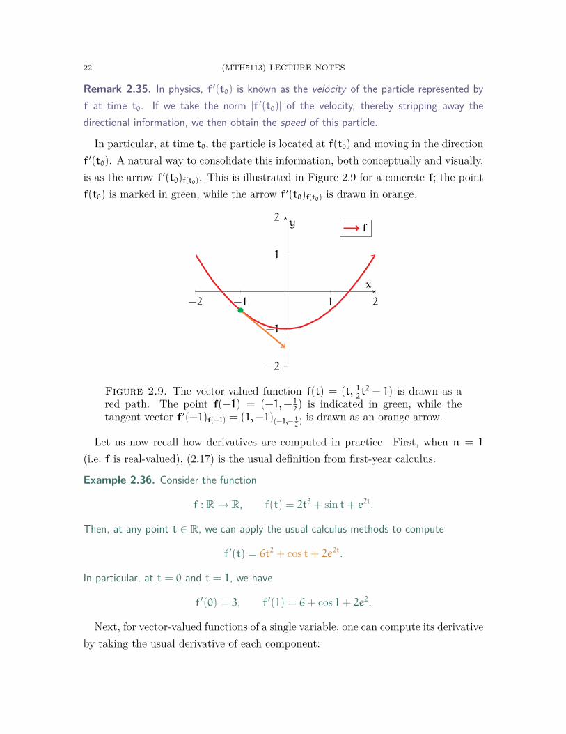
In particular, at time t0, the particle is located at f(t0) and moving in the directionf ′(t0). A natural way to consolidate this information, both conceptually and visually,is as the arrow f ′(t0)f(t0). This is illustrated in Figure 2.9 for a concrete f; the pointf(t0) is marked in green, while the arrow f ′(t0)f(t0) is drawn in orange.
−2 −1 1 2
−2
−1
1
2
x
yf
Figure 2.9. The vector-valued function f(t) = (t, 12t2 − 1) is drawn as a
red path. The point f(−1) = (−1,− 12) is indicated in green, while the
tangent vector f ′(−1)f(−1) = (1,−1)(−1,− 12) is drawn as an orange arrow.
Let us now recall how derivatives are computed in practice. First, when n = 1
(i.e. f is real-valued), (2.17) is the usual definition from first-year calculus.
Example 2.36. Consider the function
f : R → R, f(t) = 2t3 + sin t+ e2t.
Then, at any point t ∈ R, we can apply the usual calculus methods to compute
f ′(t) = 6t2 + cos t+ 2e2t.
In particular, at t = 0 and t = 1, we have
f ′(0) = 3, f ′(1) = 6+ cos 1+ 2e2.
Next, for vector-valued functions of a single variable, one can compute its derivativeby taking the usual derivative of each component:

(MTH5113) LECTURE NOTES 23
Theorem 2.37. Let f be as in Definition 2.34, and write f in terms of its components:
f = (f1, f2, . . . , fn), fk : I → R, 1 ≤ k ≤ n.
Then, for any t0 ∈ I, we have that
(2.19) f ′(t0) = (f ′1(t0), f′2(t0), . . . , f
′n(t0)),
as long as each of f ′1(t0), . . . , f ′n(t0) exists.
Proof. By the definitions of vector addition and scalar multiplication, we havef(t) − f(t0)
t− t0=
(f1(t) − f1(t0)
t− t0, . . . ,
fn(t) − fn(t0)
t− t0
).
Also, by Theorem 2.27, the limits of the above are also taken componentwise,
limt→t0
f(t) − f(t0)
t− t0=
(limt→t0
f1(t) − f1(t0)
t− t0, . . . , lim
t→t0
fn(t) − fn(t0)
t− t0
)= (f ′1(t0), . . . , f
′n(t0)),
which yields the desired formula (2.19). □
Thus, finding derivatives of vector-valued functions is not any more difficult thanbefore; one just has to apply the usual steps from first-year calculus multiple times.
Example 2.38. Consider the function γ from Example 2.21,
γ : R → R2, γ(t) = (cos t, sin t),
and let us compute its derivative at any t ∈ R. By Theorem 2.37, we need only computethe derivatives of the components cos t and sin t of γ:
γ ′(t) =
(d
dt(cos t), d
dt(sin t)
)= (− sin t, cos t).
To get a better visual sense of what is happening, we find γ and γ ′ at specific points:
t 0 π4
π2
3π4
π
γ(t) (1, 0)(
1√2, 1√
2
)(0, 1)
(− 1√
2, 1√
2
)(−1, 0)
γ ′(t) (0, 1)(− 1√
2, 1√
2
)(−1, 0)
(− 1√
2,− 1√
2
)(0,−1)
The image of γ is drawn (in red) in the left part of Figure 2.10. The values of γ(t) inthe above table are drawn in green; the tangent vectors γ ′(t)γ(t) are drawn in blue.

24 (MTH5113) LECTURE NOTES
−1 1
−1
1
x
y γ
−11 2 3
−2
2
2
4
x
y
z γ
Figure 2.10. The left plot contains the image of γ from Example 2.38,while the right plot contains the image of γ from Example 2.39 (both inred). Both plots contain some sample values of γ(t) (in green), as well asthe corresponding tangent vectors γ ′(t)γ(t) (in blue).
Example 2.39. Consider next the function
γ : (−2, 2) → R3, γ(t) = (t2 + 1, t, et).
Again, to find γ ′, we simply differentiate each component separately:
γ ′(t) =
(d
dt(t2 + 1),
d
dtt,
d
dtet)
= (2t, 1, et).
Some specific values of γ and γ ′ are given in the following table:
t −1 − 12
0 12
1
γ(t) (2,−1, e−1)(
54,− 1
2, e−
12
)(1, 0, 1)
(54, 12, e
12
)(2, 1, e)
γ ′(t) (−2, 1, e−1)(−1, 1, e−
12
)(0, 1, 1)
(1, 1, e
12
)(2, 1, e)
A plot of γ, along with the points γ(t) and the arrows γ ′(t)γ(t) from the above table,can be found in the right drawing of Figure 2.10.
Example 2.40. For a more abstract example, let us fix p, v ∈ Rn and define
ℓ : R → Rn, ℓ(t) = p+ tv.
Note first that ℓ(0) = p, so the image of ℓ passes through the point p.Next, writing out p and v in terms of their components, we have that
ℓ(t) = (p1 + tv1, . . . , pn + tvn), ℓ ′(t) = (v1, . . . , vn) = v,
(MTH5113) LECTURE NOTES 25
since the only non-constant quantity in the above is t. Thus, we see that ℓ is alwaysmoving in the (constant) direction v. Combining all the above, we conclude that ℓ mapsout the line in Rn through p and along the direction v.
As the above examples 2.38 might suggest, vector-valued functions of a single vari-able will form the foundations for our study of curves later on in this module.
2.6. Open and Connected Sets. We now turn our attention to functions of mul-tiple variables. Before discussing how such functions can be differentiated, let us firstpose and answer the following more foundational question:
Question 2.41. Consider a function f : U → Rn, where U is a subset of Rm. Whatassumptions do we need on U in order to make sense of derivatives of f?
Suppose we wish to differentiate f at a point p ∈ U. As you know, finding deriva-tives corresponds to measuring how f is changing at p. However, to understand this,we must measure how f behaves near p. Therefore, it makes sense to differentiate f
at p only when f is also defined at points nearby p.In other words, the crucial property needed for the domain U of f is the following:
whenever p ∈ U, and whenever q is “sufficiently close” to p, then q must also be inU. This property is captured mathematically via the concept of openness:
Definition 2.42. A subset U of Rm is open iff for any p ∈ U, there exists some δ > 0
such that if q ∈ Rn satisfies |q− p| < δ, then q ∈ U as well.
The formal Definition 2.42, which could seem intimidating at first, can be directlyconnected to the prior discussion. In particular, δ corresponds to a “small enoughdistance” from p, while the points q represent those that are “sufficiently close” top, measured in terms of our threshold δ. Putting this all together, Definition 2.42states that if you start from a point p ∈ U, and you take a sufficiently small stepaway from p (of distance less than δ), then you will not leave the set U.
One can also think of an open subset U ⊆ Rm as one that does not contain any ofits boundary, or edge, points. Intuitively, if p ∈ U lies on the edge of U, then one cantake as small a step as one wishes in some direction and end up outside of U.
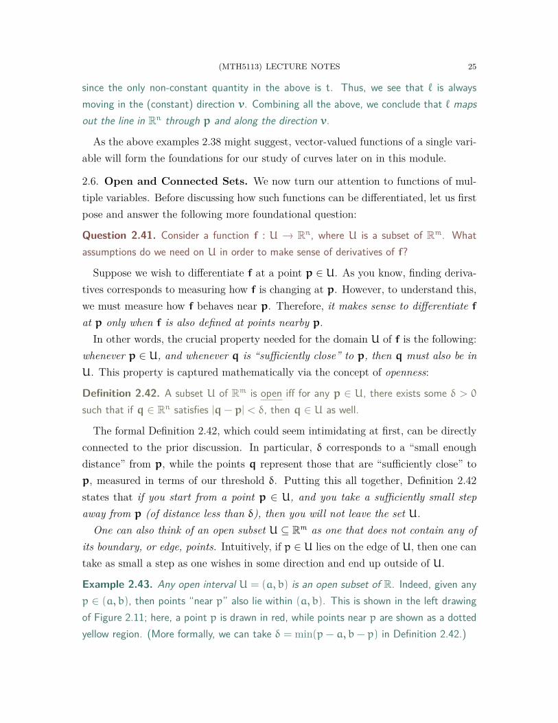
Example 2.43. Any open interval U = (a, b) is an open subset of R. Indeed, given anyp ∈ (a, b), then points “near p” also lie within (a, b). This is shown in the left drawingof Figure 2.11; here, a point p is drawn in red, while points near p are shown as a dottedyellow region. (More formally, we can take δ = min(p− a, b− p) in Definition 2.42.)

26 (MTH5113) LECTURE NOTES
On the other hand, a closed interval A = [a, b] is not an open subset of R. To showthis, we consider the boundary point a ∈ A; see the right drawing in Figure 2.11. Noteany point to the left of a does not lie in A, no matter how close it is to a. In other words,the dotted green region in Figure 2.11, representing points “close to a”, must containpoints that do not lie in A. Thus, A violates the conditions of Definition 2.42.
Upa b
A
a b
Figure 2.11. The drawings show the open interval U (left) and the closedinterval A (right) from Example 2.43. In the left picture, given a pointp ∈ U (in red), one can find a neighbourhood of p (e.g. the dotted yellowregion) that is contained in U. On the other hand, in the right graphic,for the point a at the boundary of A, any neighbourhood of a (such as thedotted green region) must contain a point that is not in A.
R
p
B(p0, r)
p0
r
p
B(p0, r)
p0
r
p
Figure 2.12. The left graphic depicts the open rectangle R (in blue andgreen) from Example 2.44(2); given some p ∈ R (drawn in red), one canfind a disk around p (in grey) that is contained in U. Similarly, the middlegraphic shows the open disk from Example 2.44(3). The drawing on theright shows a closed disk, which is not open; in particular, the point p (inred) on the boundary of B(p0, r) violates Definition 2.42.
Example 2.44. The following subsets of R2 are open:(1) The unit open disk about the origin:
B(0, 1) = {(x, y) ∈ R2 | x2 + y2 < 1}.
(2) Any open rectangle:
R = (a, b)× (c, d) = {(x, y) ∈ R2 | a < x < b, c < y < d}.
(3) Any open disk, with centre p0 ∈ R2 and radius r > 0:
B(p0, r) = {p ∈ R2 | |p− p0| < r}.
(MTH5113) LECTURE NOTES 27
On the other hand, every closed disk,
B(p0, r) = {p ∈ R2 | |p− p0| ≤ r},
is not an open subset of R2. See Figure 2.12 for illustrations.
Example 2.45. The ideas in Example 2.44 generalise to all dimensions. For instance,given any centre p0 ∈ Rm and radius r > 0, we can define the open and closed balls
B(p0, r) = {p ∈ Rm | |p− p0| < r}, B(p0, r) = {p ∈ Rm | |p− p0| ≤ r},
respectively. Again, B(p0, r) is an open subset of Rm, while B(p0, r) fails to be open.
There is another requirement, in addition to openness, that we can adopt to simplifymatters. Notice that in the definition of the derivative (Definition 2.34), the domainI of the function was assumed to be an open interval. While Example 2.43 showedthat I is an open subset of R, one also has another observation:
• I is connected—more specifically, given any pair of points on I, the line segmentconnecting these two points also lies within I.
The reason for wanting connectedness is mainly a matter of convenience. Supposeinstead that I is a union of disjoint open intervals, for example,
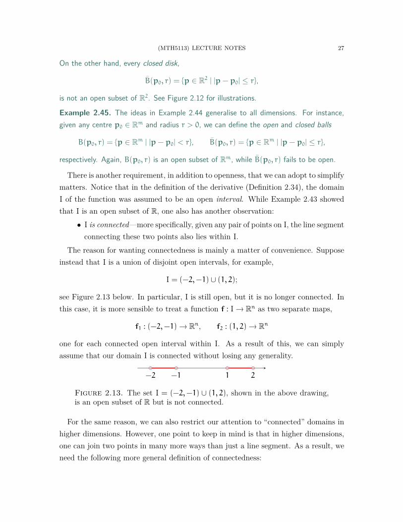
I = (−2,−1) ∪ (1, 2);
see Figure 2.13 below. In particular, I is still open, but it is no longer connected. Inthis case, it is more sensible to treat a function f : I → Rn as two separate maps,
f1 : (−2,−1) → Rn, f2 : (1, 2) → Rn
one for each connected open interval within I. As a result of this, we can simplyassume that our domain I is connected without losing any generality.
−2 −1 1 2
Figure 2.13. The set I = (−2,−1) ∪ (1, 2), shown in the above drawing,is an open subset of R but is not connected.
For the same reason, we can also restrict our attention to “connected” domains inhigher dimensions. However, one point to keep in mind is that in higher dimensions,one can join two points in many more ways than just a line segment. As a result, weneed the following more general definition of connectedness:
28 (MTH5113) LECTURE NOTES
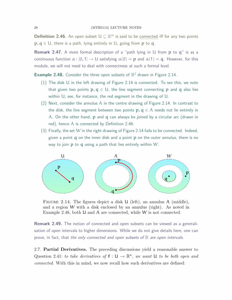
Definition 2.46. An open subset U ⊆ Rm is said to be connected iff for any two pointsp,q ∈ U, there is a path, lying entirely in U, going from p to q.
Remark 2.47. A more formal description of a “path lying in U from p to q” is as acontinuous function α : [0, 1] → U satisfying α(0) = p and α(1) = q. However, for thismodule, we will not need to deal with connectness at such a formal level.
Example 2.48. Consider the three open subsets of R2 drawn in Figure 2.14.(1) The disk U in the left drawing of Figure 2.14 is connected. To see this, we note
that given two points p,q ∈ U, the line segment connecting p and q also lieswithin U; see, for instance, the red segment in the drawing of U.
(2) Next, consider the annulus A in the centre drawing of Figure 2.14. In contrast tothe disk, the line segment between two points p,q ∈ A needs not lie entirely inA. On the other hand, p and q can always be joined by a circular arc (drawn inred), hence A is connected by Definition 2.46.
(3) Finally, the set W in the right drawing of Figure 2.14 fails to be connected. Indeed,given a point q on the inner disk and a point p on the outer annulus, there is noway to join p to q using a path that lies entirely within W.
U
p
q
Ap
q
W
p
q
Figure 2.14. The figures depict a disk U (left), an annulus A (middle),and a region W with a disk enclosed by an annulus (right). As noted inExample 2.48, both U and A are connected, while W is not connected.
Remark 2.49. The notion of connected and open subsets can be viewed as a generali-sation of open intervals to higher dimensions. While we do not give details here, one canprove, in fact, that the only connected and open subsets of R are open intervals.
2.7. Partial Derivatives. The preceding discussions yield a reasonable answer toQuestion 2.41: to take derivatives of f : U → Rn, we want U to be both open andconnected. With this in mind, we now recall how such derivatives are defined:

(MTH5113) LECTURE NOTES 29
Definition 2.50. Let U ⊆ Rm be both open and connected, let f : U → Rn, and letp = (p1, . . . , pm) ∈ U. Then, given any 1 ≤ k ≤ m, we define the partial derivativewith respect to the k-th variable of f at p to be
(2.20) ∂kf(p) = limq→pk
f(p1, . . . , q, . . . , pm) − f(p1, . . . , pk, . . . , pm)
q− pk
,
whenever the limit on the right-hand side of (2.20) exists.Moreover, whenever ∂kf(p) exists for every p ∈ U, we define the corresponding partial
derivative of f to be the function ∂kf : U → Rn mapping each p ∈ U to ∂kf(p).
Remark 2.51. Note that when m = 1 in Definition 2.50, the partial derivative ∂1f(p) isthe same as the ordinary derivative f ′(p) from Definition 2.34.
First, when n = 1 in Definition 2.50 (that is, f is real-valued), the partial derivativesof f can be computed using the methods you previously learned in calculus:
Example 2.52. Consider the real-valued function
h : R2 → R, h(u, v) = u+ v2 + u3v.
To compute the partial derivative ∂1h, we treat the second variable v as a constant, andwe differentiate as usual (see Example 2.36) with respect to the first variable u:
∂1h(u, v) = 1+ 3u2v.
Similarly, to compute ∂2h, we hold u constant and differentiate with respect to v:
∂2h(u, v) = 2v+ u3.
Furthermore, at (u, v) = (1, 1), the partial derivatives of h evaluate to
∂1h(1, 1) = 4, ∂2h(1, 1) = 3.
Next, we turn our attention to general vector-valued functions:
Theorem 2.53. Let f be as in Definition 2.50, and write f in terms of its components:
f = (f1, f2, . . . , fn), fl : U → R, 1 ≤ l ≤ n.
Then, for any 1 ≤ k ≤ m and p ∈ U, we have that
(2.21) ∂kf(p) = (∂kf1(p), ∂kf2(p), . . . , ∂kfn(p)),
as long as each of ∂kf1(p), . . . , ∂kfn(p) exists.
30 (MTH5113) LECTURE NOTES
Proof. This is analogous to the proof of Theorem 2.37. We again use that vectoraddition, scalar multiplication, and limits are all evaluated componentwise. □
Theorem 2.53 shows there is nothing novel in taking partial derivatives of a vector-valued function f—you simply apply the usual tricks to each component of f.
Example 2.54. Consider the function
f : R2 → R3, f(u, v) = (uv, u+ v, sinu+ cos v).
To compute ∂1f, we simply take this partial derivative of each component of f:
∂1f(u, v) =
(∂
∂u(uv),
∂
∂u(u+ v),
∂
∂u(sinu+ cos v)
)= (v, 1, cosu).
A similar computation yields ∂2f, for each (u, v) ∈ R2:
∂2f(u, v) =
(∂
∂v(uv),
∂
∂v(u+ v),
∂
∂v(sinu+ cos v)
)= (u, 1,− sin v).
Let us now discuss now partial derivatives can be interpreted. Consider a functiong : V → Rn, with V an open subset of R2 (i.e. g is a function of two variables).
Fix a point (u0, v0) ∈ V , and let γ denote the function given by
γ(u) = g(u, v0),
that is, we fix v = v0 and vary only u in g. Then, the derivative of γ at u0 satisfies
γ ′(u0) = limu→u0
g(u, v0) − g(u0, v0)
u− u0
= ∂1g(u0, v0),
and it follows that∂1g(u0, v0)g(u0,v0) = γ ′(u0)γ(u0).
Recall that the tangent vector γ ′(u0)γ(u0) is the arrow, starting from γ(u0), thatindicates the direction and speed in which γ is changing while at parameter u = u0.Thus, from the definition of γ, we conclude: the tangent vector ∂1g(u0, v0)g(u0,v0)
represents the direction and speed at which g is changing while at (u, v) = (u0, v0),and while v is held constant and u is varied.
(MTH5113) LECTURE NOTES 31
Similarly, if we defineλ(v) = g(u0, v),
then its derivative satisfies
λ ′(v0) = limv→v0
g(u0, v) − g(u0, v0)
v− v0
= ∂2g(u0, v0).
Thus, similar to the previous case, the arrow ∂2g(u0, v0)g(u0,v0) captures how g ischanging while at (u0, v0), and while u is held constant and v is varied.
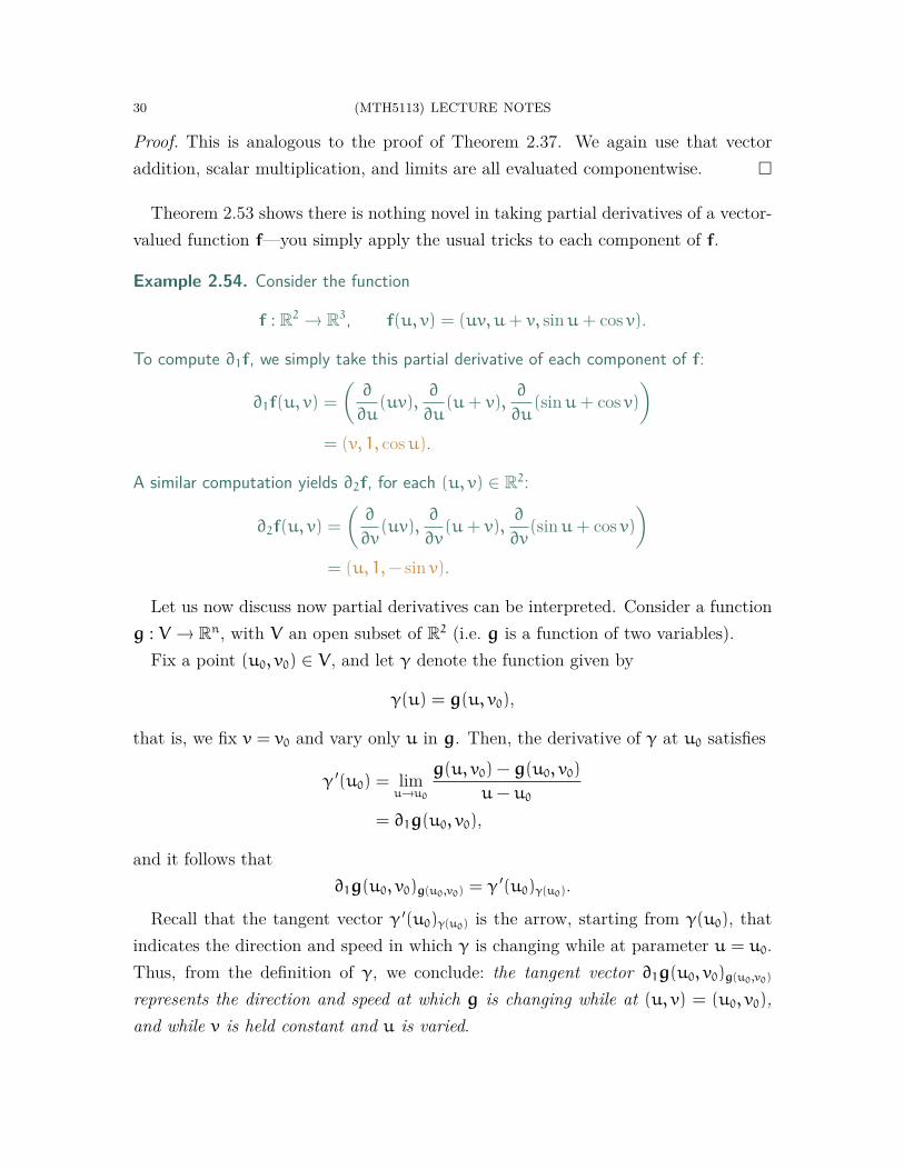
For a graphical demonstration of these curves γ and λ, see Figure 2.15 below.
−1.5 −1 −0.50.5 1
1.5−1
1
−1
1
x
y
zσ
−1.5 −1 −0.50.5 1
1.5−1
1
−1
1
x
y
zσ
Figure 2.15. The plots show σ from Example 2.55. In the left diagram,the purple curves depict paths γ obtained by holding v constant, while theorange arrows depict tangent vectors of the form ∂1σ(u, v)σ(u,v). In the rightdiagram, the green curves depict paths λ obtained by holding u constant,while the red arrows depict tangent vectors of the form ∂2σ(u, v)σ(u,v).
Example 2.55. Let us return to the cylinder from Example 2.23:
(2.22) σ : R2 → R3, σ(u, v) = (cosu, sinu, v).
See Figure 2.15 (and Figure 2.7) for illustrations of the image of σ. The purple circlesin the left drawing are obtained by holding v constant and varying u in (2.22); the greenlines in the right drawing are obtained by holding u constant and varying v in (2.22).
We can compute the partial derivatives of σ using Theorem 2.53:
∂1σ(u, v) = (− sinu, cosu, 0), ∂2σ(u, v) = (0, 0, 1).
Furthermore, the tangent vectors
∂1σ(0, 0)σ(0,0) = (0, 1, 0)(1,0,0), ∂1σ(−π
2, 1)
σ(−π2,1) = (1, 0, 0)(0,−1,1)
32 (MTH5113) LECTURE NOTES
are drawn as orange arrows in the left plot of Figure 2.15, while the tangent vectors
∂2σ(0, 0)σ(0,0) = (0, 0, 1)(1,0,0), ∂2σ(π,−1)σ(π,−1) = (0, 0, 1)(−1,0,−1)
are drawn as red arrows in the right plot of Figure 2.15.Note that, in accordance to our intuitions, the orange arrows point along the purple
paths, while the red arrows point along the green paths.
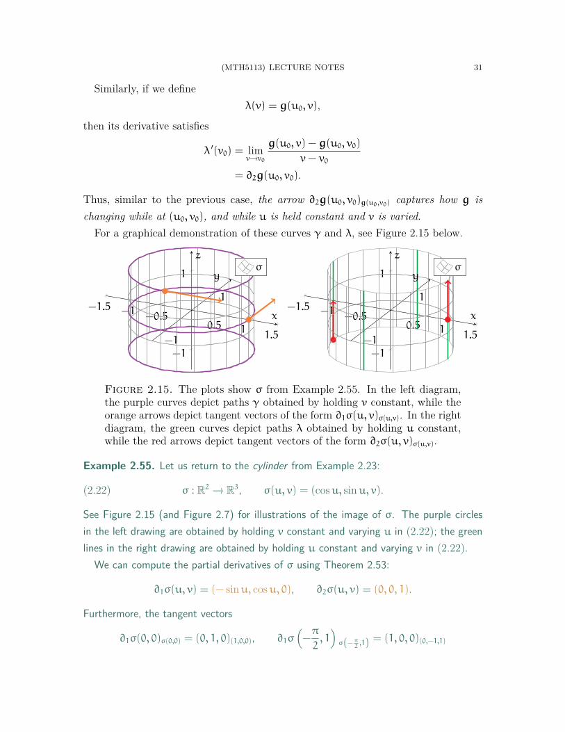
Example 2.56. Consider now the function
ρ : R2 → R3, ρ(u, v) = (u, v, u2 + v2),
whose image is a paraboloid in 3-dimensional space; see Figure 2.16.Differentiating ρ, we see that
∂1ρ(u, v) = (1, 0, 2u), ∂2ρ(u, v) = (1, 0, 2v).
In particular, at (u, v) = (0, 0), we have
∂1ρ(0, 0)ρ(0,0) = (1, 0, 0)(0,0,0), ∂2ρ(0, 0)ρ(0,0) = (0, 1, 0)(0,0,0).
These arrows are drawn in the middle and right plots of Figure 2.16, respectively.
−11
−1
1
1
2
x
y
z
ρ
−11
−1
1
1
2
x
y
z
−11
−1
1
1
2
x
y
z
Figure 2.16. The left plot shows the image of ρ from Example 2.56. Inthe middle diagram, the purple curves depict paths obtained by holding v
constant, while the orange arrow is the tangent vector ∂1ρ(0, 0)ρ(0,0). In theright diagram, the green curves depict paths obtained by holding u constant,while the red arrow is the tangent vector ∂2ρ(0, 0)ρ(0,0).
Finally, we remark that functions of two variables, such as those found in Examples2.55 and 2.56, will form the basis for our study of surfaces later in this module.
2.8. Vector Fields. We now shake things up by bringing tangent vectors back intothe discussion—we consider functions that have tangent vectors as values:
(MTH5113) LECTURE NOTES 33
Definition 2.57. Let A be a subset of Rn. A vector field on A is a function F that mapseach point p ∈ A to a tangent vector F(p) ∈ TpRn starting from p.
In other words, a vector field F maps each point p in its domain to an arrow F(p)
beginning at the same point p. This, in particular, allows for a natural way to plotvector fields. Since F(p) is a tangent vector based at p, we can depict F(p) by simplydrawing the corresponding arrow in Rn, with its starting point at p. By drawn alarge enough sample of arrows, we can gain an understanding of how F behaves.
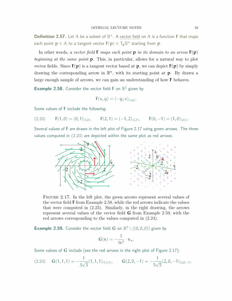
Example 2.58. Consider the vector field F on R2 given by
F(x, y) = (−y, x)(x,y).
Some values of F include the following:
(2.23) F(1, 0) = (0, 1)(1,0), F(2, 1) = (−1, 2)(2,1), F(0,−1) = (1, 0)(0,1).
Several values of F are drawn in the left plot of Figure 2.17 using green arrows. The threevalues computed in (2.23) are depicted within the same plot as red arrows.
−2 2
−2
2
x
y
−22
−2
2
−2
2
x
yz
Figure 2.17. In the left plot, the green arrows represent several values ofthe vector field F from Example 2.58, while the red arrows indicate the valuesthat were computed in (2.23). Similarly, in the right drawing, the arrowsrepresent several values of the vector field G from Example 2.59, with thered arrows corresponding to the values computed in (2.24).
Example 2.59. Consider the vector field G on R3 \ {(0, 0, 0)} given by
G(x) = −1
|x|3· x x.
Some values of G include (see the red arrows in the right plot of Figure 2.17):
(2.24) G(1, 1, 1) = −1
3√3(1, 1, 1)(1,1,1), G(2, 0,−1) = −
1
5√5(2, 0,−1)(2,0,−1).
34 (MTH5113) LECTURE NOTES
Other values of G are also drawn (in various colours) in the right part of Figure 2.17.In classical physics, G is often used to model the Newtonian gravitational force exerted
by a massive particle sitting at the origin. At any point x ∈ R3, with x 6= (0, 0, 0),the tangent vector G(x) points from x toward the origin. This is the gravitational forcecausing an object at x to accelerate toward the origin.
In addition, note that the length of G(x) satisfies
|G(x)| = |x|−2,
that is, the arrow becomes longer as x becomes closer to the origin. Thus, the gravitationalforce becomes stronger as one moves toward the particle at the origin.
Note that vector fields are hardly any different from vector-valued functions. Themain difference is cosmetic: for a vector field F, we also include p as part of the valueof F(p)—as the starting point of the tangent vector.
In other words, a vector field F can be made into a vector-valued function by takingonly the vector component of each of its values F(p). Similarly, vector-valued fuctionsare made into a vector fields by attaching a starting point to each of its values.
Remark 2.60. In fact, most calculus texts will define a vector field on Rn as just avector-valued function f : A → Rn, without any reference to tangent vectors. However,for this module, we will maintain a conceptual distinction between vector-valued functionsand vector fields, since they have rather different interpretations.
We now complete our discussion of differentiation with yet another familiar concept:gradients. However, here we adopt a slightly different definition:
Definition 2.61. Let U ⊆ Rm be open and connected, let f : U → R, and let p ∈ U.We define the gradient of f at p, denoted ∇f(p) or grad f(p), to be the tangent vector
(2.25) ∇f(p) = (∂1f(p), ∂2f(p), . . . , ∂mf(p))p ∈ TpRm,
whenever the right-hand side is well-defined.Furthermore, if ∇f(p) exists at every p ∈ U, then we define the gradient of f itself to
be the vector field mapping each p ∈ U to ∇f(p) ∈ TpRm.
Observe that the gradient of a function f aggregates all the partial derivatives off into a single object. Moreover, the values ∇f(p) are interpreted as arrows in Rm
starting at p. Later on, we will explore some geometric meanings of these arrows.
(MTH5113) LECTURE NOTES 35
Remark 2.62. In contrast to derivatives (Definition 2.34) and partial derivatives (Defi-nition 2.50), the gradient is only applied to real-valued functions.
Remark 2.63. Recall that in calculus, ∇f was (equivalently) defined to be the vector-valued function whose components are the partial derivatives of f. However, in eithercase, the values of the gradient are always interpreted as arrows.
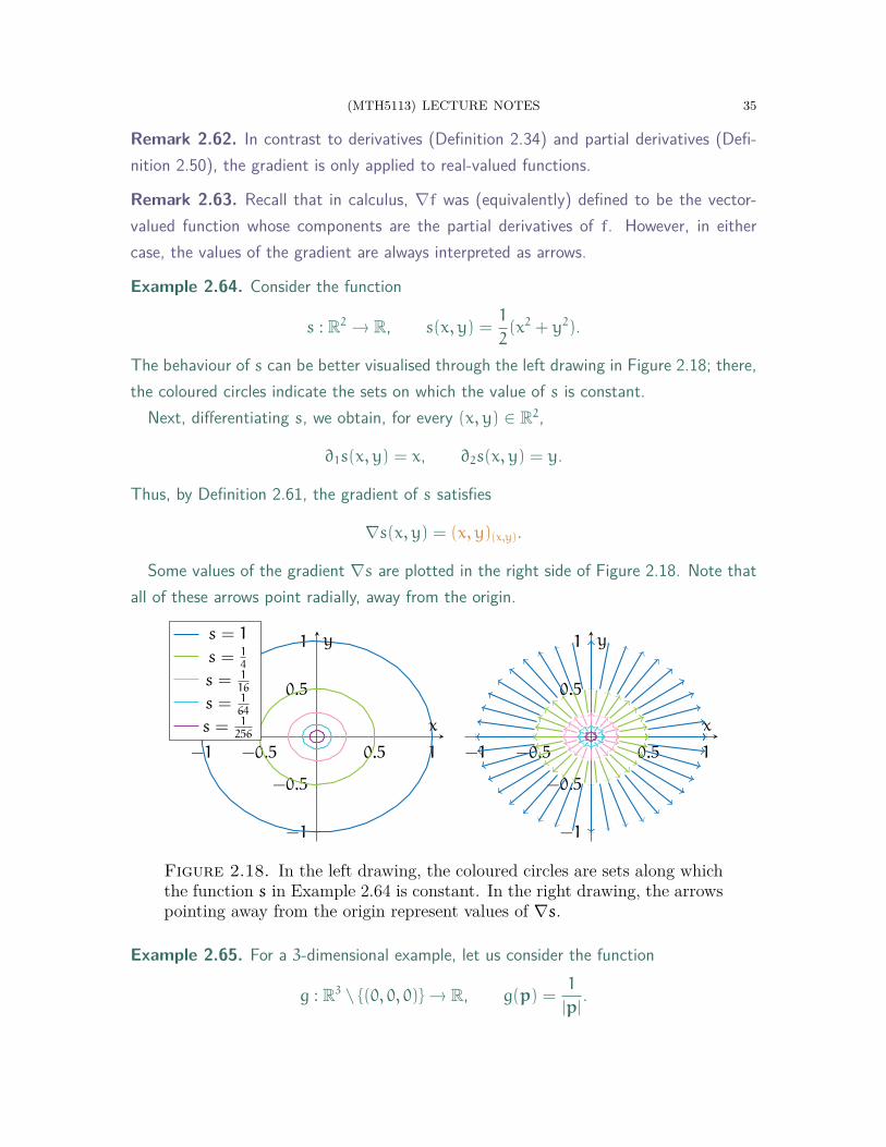
Example 2.64. Consider the function
s : R2 → R, s(x, y) =1
2(x2 + y2).
The behaviour of s can be better visualised through the left drawing in Figure 2.18; there,the coloured circles indicate the sets on which the value of s is constant.
Next, differentiating s, we obtain, for every (x, y) ∈ R2,
∂1s(x, y) = x, ∂2s(x, y) = y.
Thus, by Definition 2.61, the gradient of s satisfies
∇s(x, y) = (x, y)(x,y).
Some values of the gradient ∇s are plotted in the right side of Figure 2.18. Note thatall of these arrows point radially, away from the origin.
−1 −0.5 0.5 1
−1
−0.5
0.5
1
x
ys = 1
s = 14
s = 116
s = 164
s = 1256
−1 −0.5 0.5 1
−1
−0.5
0.5
1
x
y
Figure 2.18. In the left drawing, the coloured circles are sets along whichthe function s in Example 2.64 is constant. In the right drawing, the arrowspointing away from the origin represent values of ∇s.
Example 2.65. For a 3-dimensional example, let us consider the function
g : R3 \ {(0, 0, 0)} → R, g(p) =1
|p|.

36 (MTH5113) LECTURE NOTES
Alternatively, we can write g in terms of its component variables as
g(x, y, z) =1
|(x, y, z)|=
1√x2 + y2 + z2
.
Let us now take partial derivatives of g. First, by the chain and power rules,
∂1g(x, y, z) =
(−1
2
)1
(x2 + y2 + z2)32
· 2x
= −x
(x2 + y2 + z2)32
.
By similar calculations, we also obtain
∂2g(x, y, z) = −y
(x2 + y2 + z2)32
, ∂3g(x, y, z) = −z
(x2 + y2 + z2)32
.
Combining the above, we conclude that the gradient of g is
∇g(x, y, z) = −1
(x2 + y2 + z2)32
· (x, y, z)(x,y,z).
It is perhaps more informative to rewrite the preceding formula in vector form:
∇g(p) = −1
|p|3· pp.
Notice that ∇g equals the vector field G from Example 2.59, modelling the Newtoniangravitational force from a particle at the origin. Thus, the gravitational force G has theform of a gradient of a scalar function. In physics terminology, the scalar function −g iscalled the gravitational potential arising from this particle.
2.9. Integrals. We now turn our attention toward the other major aspect of calculus:integration. Here, we explore some interpretations of integrals, and we recall somebasic methods you learned in calculus for evaluating them.
Let us begin with integrals of single-variable functions, which you learned to com-pute in MTH4100/4200: Calculus I. First, recall that if we integrate the constantfunction 1 along an interval I = [a, b] of the real line, then we obtain∫
I
dx =
∫b
a
1 dx = b− a.
In particular, the integral of 1 over I yields the length of I.Now, one may want to alter how “length” is measured. For instance, one may be
interested in a “weighted length”, in which some points count for more than others.
(MTH5113) LECTURE NOTES 37
This is where the power of integration comes in—given g : I → R, we can interpret∫I
gdx =
∫b
a
g(x)dx
as a “weighted length” of I, where the “weight” applied to any x ∈ I is given by g(x).The term “weighted length” is left deliberately vague, as it can have many different
meanings. We briefly mention a couple interpretations here:
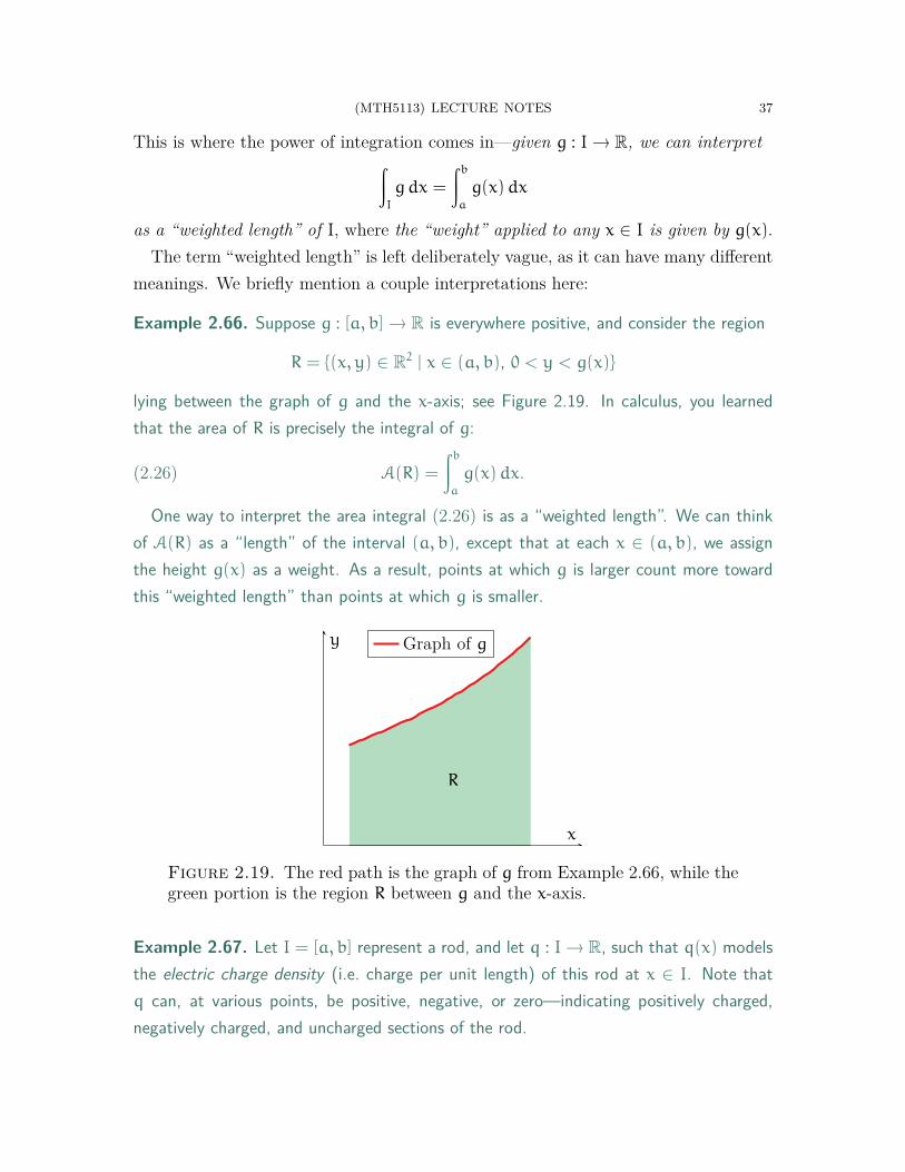
Example 2.66. Suppose g : [a, b] → R is everywhere positive, and consider the region
R = {(x, y) ∈ R2 | x ∈ (a, b), 0 < y < g(x)}
lying between the graph of g and the x-axis; see Figure 2.19. In calculus, you learnedthat the area of R is precisely the integral of g:
(2.26) A(R) =
∫b
a
g(x)dx.
One way to interpret the area integral (2.26) is as a “weighted length”. We can thinkof A(R) as a “length” of the interval (a, b), except that at each x ∈ (a, b), we assignthe height g(x) as a weight. As a result, points at which g is larger count more towardthis “weighted length” than points at which g is smaller.
R
x
y Graph of g
Figure 2.19. The red path is the graph of g from Example 2.66, while thegreen portion is the region R between g and the x-axis.
Example 2.67. Let I = [a, b] represent a rod, and let q : I → R, such that q(x) modelsthe electric charge density (i.e. charge per unit length) of this rod at x ∈ I. Note thatq can, at various points, be positive, negative, or zero—indicating positively charged,negatively charged, and uncharged sections of the rod.
38 (MTH5113) LECTURE NOTES
The total charge Q of the rod can then be found by “summing up” its density along I:
Q =
∫b
a
q(x)dx.
In particular, contributions to the total charge from parts of I where q is positive can becancelled by other contributions from areas where q is negative.
Remark 2.68. While we discussed many interpretations of integrals, we have not yetprovided a precise definition of integrals. Unfortunately, this is a more involved topic thatis beyond this module. One rigorous definition is discussed in MTH5105: Differential andIntegral Analysis. An even more powerful theory of integration (i.e. Lebesgue integration)is covered in the postgraduate module MTH716U: Measure Theory and Probability.
Next, we briefly revise how integrals of single-variable functions are calculated. Themain tool, as you probably remember, is the fundamental theorem of calculus:
Theorem 2.69 (Fundamental theorem of calculus). Let f : [a, b] → R be continuous,and assume that its derivative f ′(x) is defined for all x ∈ (a, b). Then,
(2.27)∫b
a
f ′(x)dx = f(b) − f(a).
The fundamental theorem of calculus is quite remarkable for multiple reasons. Onthe conceptual side, it establishes that differentiation and integration are inverses ofeach other—applying one operation undoes the other one.
Furthermore, the fundamental theorem of calculus provides practical ways to com-pute many integrals. The equation (2.27) relates integrals directly to derivatives, forwhich we already have many computational tricks. Therefore, if you know how todifferentiate many functions, then you can also integrate many functions!
Example 2.70. Consider the function
f : [0, π] → R, f(x) = x3 + sin x.
Note f is the derivative of
g : [0, π] → R, g(x) =1
4x4 − cos x.
Thus, applying Theorem 2.69, we see that∫π
0
(x3 + sin x)dx =
∫π
0
g ′(x)dx
(MTH5113) LECTURE NOTES 39
= g(π) − g(0)
=1
4π4 + 2.
In calculus, you have learned many methods for evaluating integrals. We will notcover most of these tricks in the lecture notes, as they are not directly relevant to thismodule. However, you can refer to your old notes and textbook [10] if needed.
2.10. Multiple Integrals. We conclude our revisions by discussing integrating func-tions of multiple variables. The first task is to extend our interpretations of single-variable integrals to double and triple integrals.
Consider a subset B ⊆ R2. Recall that, similar to the single integral case, if weintegrate the constant function 1 over B, then we obtain the area of B:
(2.28)∫∫
B
dA = A(B).
Similarly, for a subset C ⊆ R3, the integral of 1 over C yields the volume of C:
(2.29)∫∫∫
C
dV = V(C).
We can then think of general double and triple integrals as abstract measures of“weighted area” and “weighted volume”. More specifically, given
f : B → R, g : C → R,
the integrals ∫∫B
f dA,∫∫∫
C
gdV
give a weighted area and volume of B and C, with weights f and g, respectively.
Remark 2.71. In fact, one cannot define area or volume for all subsets of R2 or R3,respectively. (Look up the Banach–Tarski paradox!) One consequence of this is that wecan only integrate over what are called measurable subsets of R2 or R3. However, inpractice, any set that we encounter in this module (and in most other modules) will bemeasurable, so we do not stress about this point here.
Again, the meanings of “weighted area” and “weighted volume” are left vague inorder to emphasise their applicability to a wide variety of situations.
Example 2.72. Let B ⊆ R2 represent a plate, and let m : B → R, with m(x, y) beingthe mass density (i.e. mass per unit area) of the plate at the position (x, y) ∈ B. We can
40 (MTH5113) LECTURE NOTES
then view the total mass M of the plate as a type of “weighted area”:
M =
∫∫B
mdA.
Example 2.73. For an example in R3, we turn to quantum mechanics. Let Ψ : R3 → Cbe the wave function of a particle, which describes its present state. In this context, thequantity |Ψ(x, y, z)|2 ∈ R represents the probability density of the particle at (x, y, z).
Now, consider some region C ⊆ R3 of space. Then, the total probability that theparticle is lying in C can be obtained by integrating the probability density over C:
P(C) =∫∫∫
C
|Ψ|2 dV .
The main idea behind computing double and triple integrals is to transform theminto quantities that we already know how to compute: single integrals. If you re-member your calculus, then you know this is accomplished through Fubini’s theorem,named after Italian mathematician Guido Fubini (1879–1943):
Theorem 2.74 (Fubini’s theorem). Let R denote the rectangle
R = [a, b]× [c, d] = {(x, y) ∈ R2 | a ≤ x ≤ b, c ≤ y ≤ d}.
Then, for any bounded, piecewise continuous function f : R → R,
(2.30)∫∫
R
f dA =
∫b
a
[∫d
c
f(x, y)dy
]dx =
∫d
c
[∫b
a
f(x, y)dx
]dy.
Furthermore, if Q denotes the rectangular prism
Q = [a, b]× [c, d]× [k, l] = {(x, y, z) ∈ R3 | a ≤ x ≤ b, c ≤ y ≤ d, k ≤ z ≤ l},
then for any bounded, piecewise continuous function g : Q → R,
(2.31)∫∫∫
Q
gdV =
∫ l
k
∫d
c
∫b
a
g(x, y, z)dxdydz.
Similar formulas hold if the orders of the above integrals in x, y, and z are interchanged.
In particular, (2.30) reduces a double integral into two iterated single integrals,while (2.31) converts a triple integral into three iterated integrals.
Example 2.75. Let us compute the triple integral
(2.32)∫∫∫
Q
f dV ,

(MTH5113) LECTURE NOTES 41
where Q = [0, 1]× [0, 1]× [0, 2] is a rectangular prism in R3 (see the left picture in Figure2.20), and where f : R3 → R is the function given by
f(x, y, z) = x(y+ z).
The first step is to apply (2.31) to convert (2.32) into iterated single integrals:∫∫∫Q
f dV =
∫ 2
0
∫ 1
0
∫ 1
0
x(y+ z)dxdydz.
We can now evaluate each of the single integrals, starting from the innermost one. First,we integrate x(y+ z) with respect to x (treating y and z as constants):∫ 2
0
∫ 1
0
∫ 1
0
x(y+ z)dxdydz =
∫ 2
0
∫ 1
0
(y+ z)
[∫ 1
0
xdx
]dydz
=1
2
∫ 2
0
∫ 1
0
(y+ z)dydz.
We then continue by integrating with respect to y (while holding z constant):
1
2
∫ 2
0
∫ 1
0
(y+ z)dydz =1
2
∫ 2
0
[1
2y2 + zy
]∣∣∣∣y=1
y=0
dz
=
∫ 2
0
(1
4+
1
2z
)dz.
Combining all the above and integrating with respect to z yields the solution:∫ 2
0
(1
4+
1
2z
)dz =
3
2.
0.5 11.5 2
1
21
2
Q
x
y
z
0.5 1
0.5
1
x = 1
y = 0
y = x
Tx
y
Figure 2.20. The solid figure on the left is the region Q from Example2.75, while the shaded triangle on the right is T from Example 2.76.
42 (MTH5113) LECTURE NOTES
Example 2.76. For a more involved example, let us compute the double integral∫∫T
gdA.
where T ⊆ R2 is the triangular region bounded by the lines y = 0, x = 1, and y = x (seethe right drawing in Figure 2.20), and where
g : R2 → R, g(x, y) = xy.
The main idea is to apply (2.30) to the square [0, 1]× [0, 1] (which contains T) and toreplace the integrand by another function that is equal to g on T and vanishes outside T :
gT(x, y) =
g(x, y) = xy (x, y) ∈ T ,0 otherwise.
From this, along with Fubini’s theorem, we obtain∫∫T
gdA =
∫∫[0,1]×[0,1]
gT dA
=
∫ 1
0
∫ 1
0
gT(x, y)dydx
=
∫ 1
0
[∫ x
0
xydy
]dx.
Notice that in the last step, we can restrict the domain of the inner integral, since for anyx ∈ [0, 1], the value gT(x, y) is nonzero only when 0 < y ≤ x.
We can now evaluate the inner integral by treating x as a constant:∫ 1
0
[∫ x
0
xydy
]dx =
∫ 1
0
x
[1
2y2
]∣∣∣∣y=x
y=0
dx
=1
2
∫ 1
0
x3 dx.
The answer now follows by evaluating this last integral in x:
1
2
∫ 1
0
x3 dx =1
8.
Example 2.77. In Example 2.76, we integrated first in y and then in x. We can obtainthe same answer with the reverse order of integration, provided we describe T correctly:∫∫
T
gdA =
∫ 1
0
∫ 1
0
gT(x, y)dxdy
(MTH5113) LECTURE NOTES 43
=
∫ 1
0
∫ 1
y
xydxdy.
Indeed, evaluating the above iterated integral, we obtain∫ 1
0
∫ 1
y
xydxdy =1
2
∫ 1
0
y(1− y2)dy
=1
8.
Example 2.78. For a more abstract example, we return to the region R from Example2.66, containing the points lying between the x-axis and the graph of a positive functiong : [a, b] → R (see Figure 2.19 for an illustration).
First, the area of R is simplyA(R) =
∫∫R
dA.
Like in Examples 2.76 and 2.77, this double integral can be expanded using (2.30):∫∫R
dA =
∫b
a
[∫g(x)
0
1 dy
]dx
=
∫b
a
g(x)dx.
In particular, this justifies the calculus formula (2.26) for the area of R.
Again, we will not cover all the various tips and tricks you learned from calculusto compute multiple integrals, as this is not the main focus of the module. An usual,you can consult your calculus notes or textbook [10] for additional details.
Finally, we remark that all of the preceding discussions for double and triple inte-grals extend directly to integrals involving functions of four or more variables. How-ever, we will not encounter any such higher-dimensional integrals in this module.
44 (MTH5113) LECTURE NOTES
3. The Geometry of Curves
With revisions behind us, we now advance to the main geometric topics. Thischapter represents the first half of this effort, covering the differential geometry ofcurves. These are the simplest geometric objects that we will study, and they serveas warm-up for our future discussions involving surfaces.
You probably already have some solid intuitions for what a curve is. For example,you may visualise a curve as a string tracing out some path, or as a trajectory tracedout by a particle over time. On the other hand, if you think more abstractly, thenperhaps you view them as “1-dimensional objects” of some sort.
As written, these intuitions are too vague for a careful mathematical study. There-fore, the first major question we will need to address is the following:
Question 3.1. When we say “curve”, what exactly do we mathematically mean?
3.1. Parametric Curves. Let us begin with this vague idea of curves being particletrajectories or general “1-dimensional objects”. Recall from the previous chapter thatparticle trajectories are modelled by vector-valued functions f : (a, b) → Rn, withf(t) representing the position of the particle at time t.
Moreover, you may have noticed, in prior examples, that the images of such f traceout 1-dimensional paths; see, for instance, Examples 2.38, 2.39, and 2.40. Thus, weuse such functions as the starting point of our formal discussions:
Definition 3.2. A parametric curve is a smooth vector-valued function γ : I → Rn,where n is a positive integer, and where I is an open (finite or infinite) interval.
A few remarks on Definition 3.2 are in order. First, by γ being smooth, we meanthat we can differentiate γ as many times as we like. In particular, γ has no discon-tinuities or “jagged edges” that prevent its derivative from existing at any t ∈ I. Thesame is also assumed to hold for γ ′, as well as for higher derivatives of γ.
We also note the interval I in Definition 3.2 is allowed to be of any of the forms
I = (a, b), I = (−∞, b), I = (a,∞), I = R.
The idea is that since I is 1-dimensional, we expect that the set of points γ(t) mappedout by every t ∈ I should also be 1-dimensional.
Lastly, if you prefer to be more concrete, then you can assume n = 2 or n = 3 inDefinition 3.2. Almost all of our examples will be in these special cases.
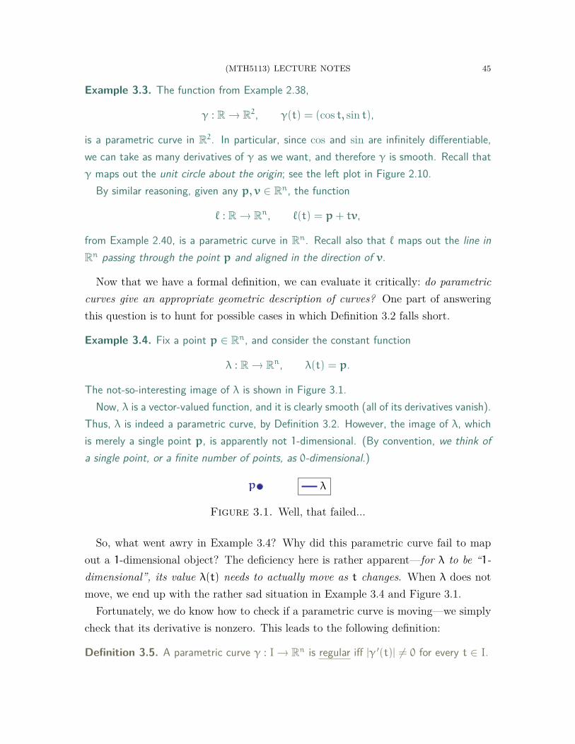
(MTH5113) LECTURE NOTES 45
Example 3.3. The function from Example 2.38,
γ : R → R2, γ(t) = (cos t, sin t),
is a parametric curve in R2. In particular, since cos and sin are infinitely differentiable,we can take as many derivatives of γ as we want, and therefore γ is smooth. Recall thatγ maps out the unit circle about the origin; see the left plot in Figure 2.10.
By similar reasoning, given any p, v ∈ Rn, the function
ℓ : R → Rn, ℓ(t) = p+ tv,
from Example 2.40, is a parametric curve in Rn. Recall also that ℓ maps out the line inRn passing through the point p and aligned in the direction of v.
Now that we have a formal definition, we can evaluate it critically: do parametriccurves give an appropriate geometric description of curves? One part of answeringthis question is to hunt for possible cases in which Definition 3.2 falls short.
Example 3.4. Fix a point p ∈ Rn, and consider the constant function
λ : R → Rn, λ(t) = p.
The not-so-interesting image of λ is shown in Figure 3.1.Now, λ is a vector-valued function, and it is clearly smooth (all of its derivatives vanish).
Thus, λ is indeed a parametric curve, by Definition 3.2. However, the image of λ, whichis merely a single point p, is apparently not 1-dimensional. (By convention, we think ofa single point, or a finite number of points, as 0-dimensional.)
p λ
Figure 3.1. Well, that failed...
So, what went awry in Example 3.4? Why did this parametric curve fail to mapout a 1-dimensional object? The deficiency here is rather apparent—for λ to be “1-dimensional”, its value λ(t) needs to actually move as t changes. When λ does notmove, we end up with the rather sad situation in Example 3.4 and Figure 3.1.
Fortunately, we do know how to check if a parametric curve is moving—we simplycheck that its derivative is nonzero. This leads to the following definition:
Definition 3.5. A parametric curve γ : I → Rn is regular iff |γ ′(t)| 6= 0 for every t ∈ I.
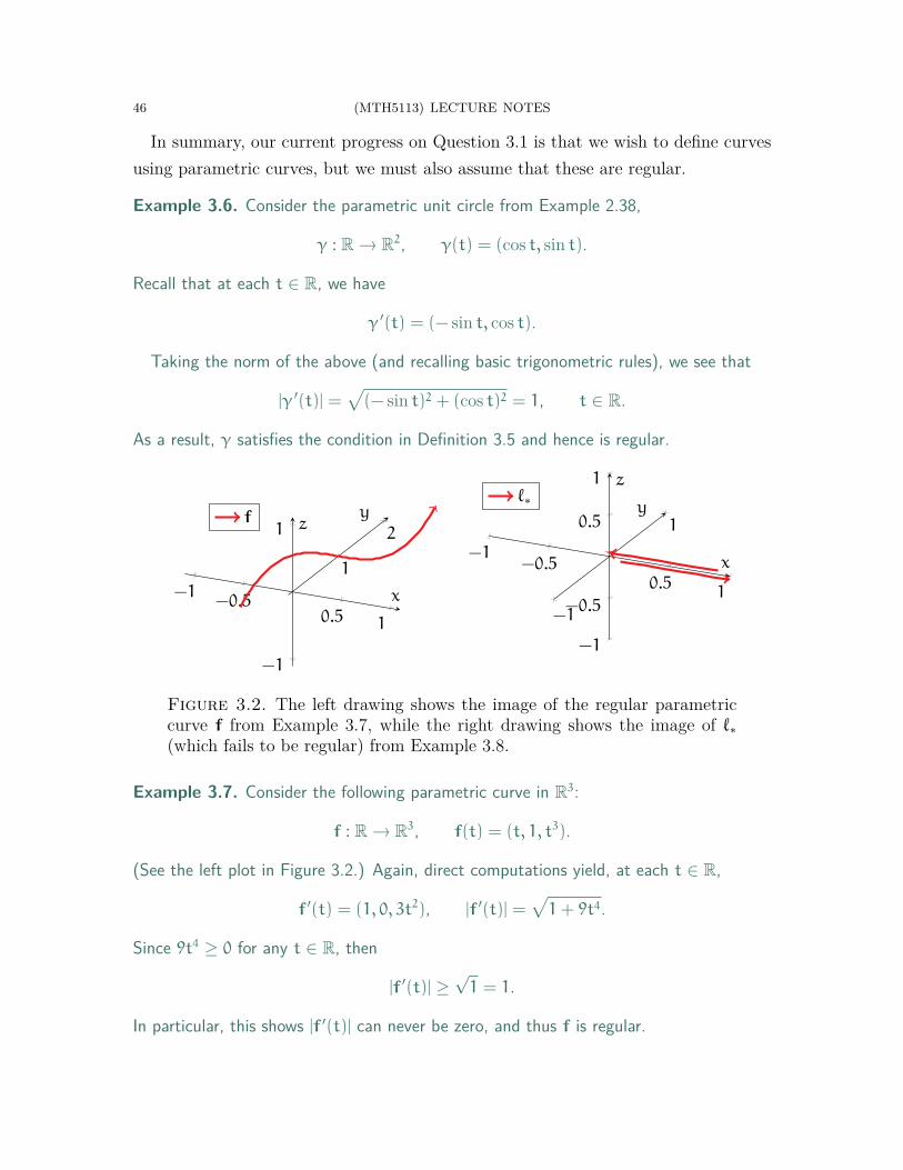
46 (MTH5113) LECTURE NOTES
In summary, our current progress on Question 3.1 is that we wish to define curvesusing parametric curves, but we must also assume that these are regular.
Example 3.6. Consider the parametric unit circle from Example 2.38,
γ : R → R2, γ(t) = (cos t, sin t).
Recall that at each t ∈ R, we have
γ ′(t) = (− sin t, cos t).
Taking the norm of the above (and recalling basic trigonometric rules), we see that
|γ ′(t)| =√
(− sin t)2 + (cos t)2 = 1, t ∈ R.
As a result, γ satisfies the condition in Definition 3.5 and hence is regular.
−1−0.5
0.5 1
1
2
−1
1
x
yzf
−1−0.5
0.51
−1
1
−1
−0.5
0.5
1
x
y
zℓ∗
Figure 3.2. The left drawing shows the image of the regular parametriccurve f from Example 3.7, while the right drawing shows the image of ℓ∗(which fails to be regular) from Example 3.8.
Example 3.7. Consider the following parametric curve in R3:
f : R → R3, f(t) = (t, 1, t3).
(See the left plot in Figure 3.2.) Again, direct computations yield, at each t ∈ R,
f ′(t) = (1, 0, 3t2), |f ′(t)| =√
1+ 9t4.
Since 9t4 ≥ 0 for any t ∈ R, then
|f ′(t)| ≥√1 = 1.
In particular, this shows |f ′(t)| can never be zero, and thus f is regular.
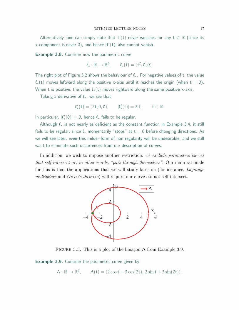
(MTH5113) LECTURE NOTES 47
Alternatively, one can simply note that f ′(t) never vanishes for any t ∈ R (since itsx-component is never 0), and hence |f ′(t)| also cannot vanish.
Example 3.8. Consider now the parametric curve
ℓ∗ : R → R3, ℓ∗(t) = (t2, 0, 0).
The right plot of Figure 3.2 shows the behaviour of ℓ∗. For negative values of t, the valueℓ∗(t) moves leftward along the positive x-axis until it reaches the origin (when t = 0).When t is positive, the value ℓ∗(t) moves rightward along the same positive x-axis.
Taking a derivative of ℓ∗, we see that
ℓ ′∗(t) = (2t, 0, 0), |ℓ ′∗(t)| = 2|t|, t ∈ R.
In particular, |ℓ ′∗(0)| = 0, hence ℓ∗ fails to be regular.Although ℓ∗ is not nearly as deficient as the constant function in Example 3.4, it still
fails to be regular, since ℓ∗ momentarily “stops” at t = 0 before changing directions. Aswe will see later, even this milder form of non-regularity will be undesirable, and we stillwant to eliminate such occurrences from our description of curves.
In addition, we wish to impose another restriction: we exclude parametric curvesthat self-intersect or, in other words, “pass through themselves”. Our main rationalefor this is that the applications that we will study later on (for instance, Lagrangemultipliers and Green’s theorem) will require our curves to not self-intersect.
−4 −2 2 4 6
−4
−2
2
4
x
yΛ
Figure 3.3. This is a plot of the limaçon Λ from Example 3.9.
Example 3.9. Consider the parametric curve given by
Λ : R → R2, Λ(t) = (2 cos t+ 3 cos(2t), 2 sin t+ 3 sin(2t)) .

48 (MTH5113) LECTURE NOTES
The image of Λ, illustrated in Figure 3.3, is known as a limaçon. Note this image passesthrough itself at the single point marked in green:
(−3, 0) = Λ(t±), t± = cos−1
(−1
3
)≈ π± 1.23.
Even if a parametric curve is regular, this alone does not prevent self-intersectionsfrom occurring. Thus, to rule out objects like Λ from Example 3.9, we will have toimpose further restrictions in our eventual definition of curves.
Remark 3.10. We emphasise that our exclusion of self-intersections is a choice made forthis module, not a necessity. In fact, much of the literature does allow for self-intersectingcurves (known as immersed curves), which have a rich theory of their own.
3.2. Reparametrisations. Thus far, we have argued that “good” parametric curvesshould be regular and should not pass through themselves. Now, we ask what othershortcomings do parametric curves have, with regards to describing geometric curves?
The following example highlights a more subtle issue:
Example 3.11. Consider the following two parametric curves:
γ1 : (0, π) → R2, γ1(t) = (cos t, sin t),
γ2 : (−1, 1) → R2, γ2(t) =(−t,
√1− t2
).
The images of γ1 and γ2 are drawn in the left and right illustrations in Figure 3.4. Observethat γ1 is regular by the computations in Example 3.6. Moreover, γ2 is regular, since
γ ′2(t) =
(−1,−
t√1− t2
)is clearly nonzero for every t ∈ (−1, 1).
Now, γ1 and γ2 are apparently different parametric curves. On the other hand, Figure3.4 shows that γ1 and γ2 trace out exactly the same points, the upper half-circle, and inthe same order. Thus, in this sense, γ1 and γ2 are not so different after all!
If you think of γ1 and γ2 in Example 3.11 as travelling particles, then this simplymeans the two particles are traversing the same path at different times and speeds.From this perspective, it is sensible to think of γ1 and γ2 as distinct.
However, we are presently concerned with questions of geometry—of shapes andsizes. Here, γ1 and γ2 both trace out the same points and hence have the same shape
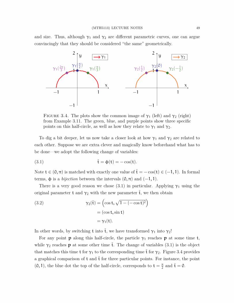
(MTH5113) LECTURE NOTES 49
and size. Thus, although γ1 and γ2 are different parametric curves, one can argueconvincingly that they should be considered “the same” geometrically.
−1 1
−1
1
2
γ1(π3)
γ1(π2)
γ1(2π3)
x
y γ1
−1 1
−1
1
2
γ2(−12)
γ2(0)γ2(12)
x
y γ2
Figure 3.4. The plots show the common image of γ1 (left) and γ2 (right)from Example 3.11. The green, blue, and purple points show three specificpoints on this half-circle, as well as how they relate to γ1 and γ2.
To dig a bit deeper, let us now take a closer look at how γ1 and γ2 are related toeach other. Suppose we are extra clever and magically know beforehand what has tobe done—we adopt the following change of variables:
(3.1) t = ϕ(t) = − cos(t).
Note t ∈ (0, π) is matched with exactly one value of t = − cos(t) ∈ (−1, 1). In formalterms, ϕ is a bijection between the intervals (0, π) and (−1, 1).
There is a very good reason we chose (3.1) in particular. Applying γ1 using theoriginal parameter t and γ2 with the new parameter t, we then obtain
γ2(t) =(
cos t,√
1− (− cos t)2)
(3.2)
= (cos t, sin t)
= γ1(t).
In other words, by switching t into t, we have transformed γ1 into γ2!For any point p along this half-circle, the particle γ1 reaches p at some time t,
while γ2 reaches p at some other time t. The change of variables (3.1) is the objectthat matches this time t for γ1 to the corresponding time t for γ2. Figure 3.4 providesa graphical comparison of t and t for three particular points. For instance, the point(0, 1), the blue dot the top of the half-circle, corresponds to t = π
2and t = 0.
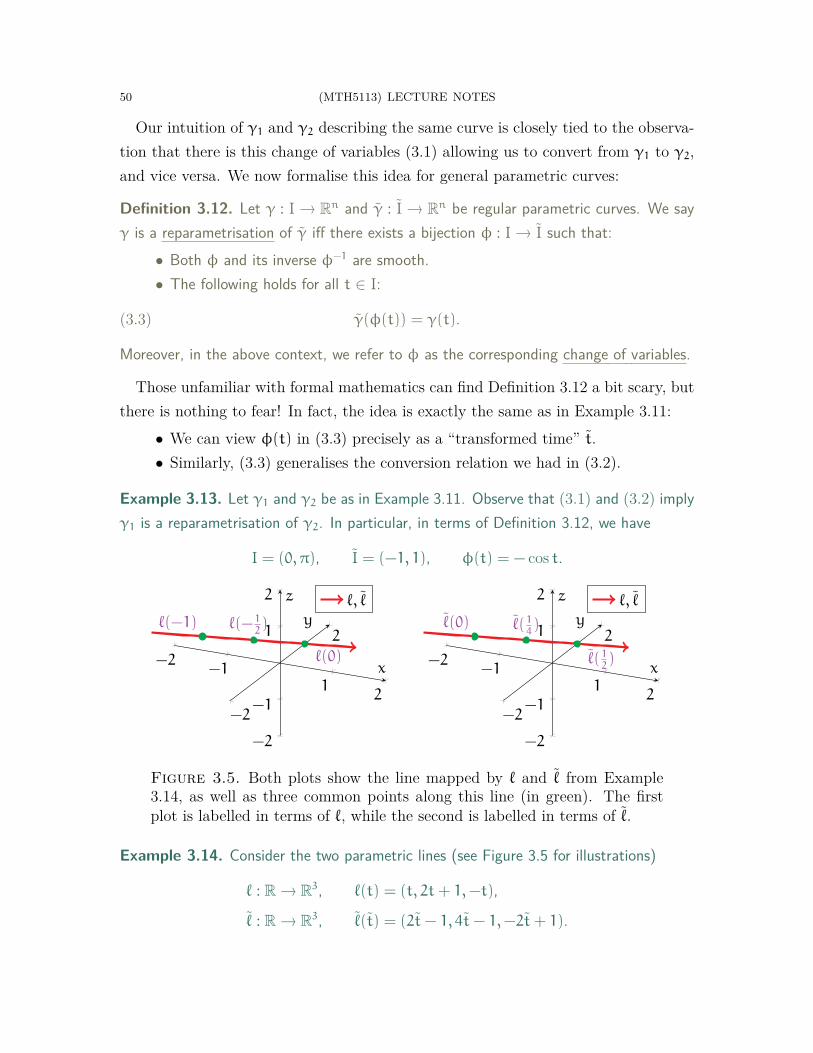
50 (MTH5113) LECTURE NOTES
Our intuition of γ1 and γ2 describing the same curve is closely tied to the observa-tion that there is this change of variables (3.1) allowing us to convert from γ1 to γ2,and vice versa. We now formalise this idea for general parametric curves:
Definition 3.12. Let γ : I → Rn and γ : I → Rn be regular parametric curves. We sayγ is a reparametrisation of γ iff there exists a bijection ϕ : I → I such that:
• Both ϕ and its inverse ϕ−1 are smooth.• The following holds for all t ∈ I:
(3.3) γ(ϕ(t)) = γ(t).
Moreover, in the above context, we refer to ϕ as the corresponding change of variables.
Those unfamiliar with formal mathematics can find Definition 3.12 a bit scary, butthere is nothing to fear! In fact, the idea is exactly the same as in Example 3.11:
• We can view ϕ(t) in (3.3) precisely as a “transformed time” t.• Similarly, (3.3) generalises the conversion relation we had in (3.2).
Example 3.13. Let γ1 and γ2 be as in Example 3.11. Observe that (3.1) and (3.2) implyγ1 is a reparametrisation of γ2. In particular, in terms of Definition 3.12, we have
I = (0, π), I = (−1, 1), ϕ(t) = − cos t.
−2−1
12
−2
2
−2
−1
1
2
ℓ(−1) ℓ(− 12)
ℓ(0)x
y
z ℓ, ℓ
−2−1
12
−2
2
−2
−1
1
2
ℓ(0) ℓ( 14)
ℓ( 12)
x
y
z ℓ, ℓ
Figure 3.5. Both plots show the line mapped by ℓ and ℓ from Example3.14, as well as three common points along this line (in green). The firstplot is labelled in terms of ℓ, while the second is labelled in terms of ℓ.
Example 3.14. Consider the two parametric lines (see Figure 3.5 for illustrations)
ℓ : R → R3, ℓ(t) = (t, 2t+ 1,−t),
ℓ : R → R3, ℓ(t) = (2t− 1, 4t− 1,−2t+ 1).
(MTH5113) LECTURE NOTES 51
We claim that ℓ is a reparametrisation of ℓ.To show this, we find the change of variables ϕ identifying ℓ with ℓ, that is, we solve
ℓ(t) = ℓ(t) for a relation between t and t. The above expands to a system of 3 equations:
t = 2t− 1, 2t+ 1 = 4t− 1, − t = −t+ 1.
By doing a bit of algebra, we then see that the above has a simulaneous solution:
(3.4) t =1
2(t+ 1).
This then inspires us to define the map
ϕ : R → R, ϕ(t) =1
2(t+ 1),
which is clearly a smooth bijection between R and itself. Moreover, its inverse satisfies
ϕ−1(t) = 2t− 1,
which is also a smooth function. Finally, from (3.4) and the above, we have that
ℓ(ϕ(t)) = ℓ(t) = ℓ(t), t ∈ R,
and hence ℓ is indeed a reparametrisation of ℓ.
The upshot, in the context of Definition 3.12, is that whenever γ is a reparametri-sation of γ, we view γ and γ as describing the same curve. This lies at the heart ofthe idea that curves, and their properties, are independent of parametrisation.
Remark 3.15. If γ is a reparametrisation of γ, then γ is also a reparametrisation of γ.We often write “γ and γ are reparametrisations of each other” due to this symmetry.
We previously mentioned that two parametric curves that are reparametrisationsof each other can be viewed as two particles traversing the same path at differentspeeds. Using a bit of calculus, we can determine how these two speeds are related:
Theorem 3.16. Let γ : I → Rn and γ : I → Rn be parametric curves. Assume γ is areparametrisation of γ, with change of variables ϕ : I → I (i.e. (3.3) holds). Then,
(3.5) γ ′(t) = ϕ ′(t) · γ ′(ϕ(t)), t ∈ I.
Proof. First, we express γ in terms of its components,
γ(t) = (γ1(t), . . . , γn(t)).
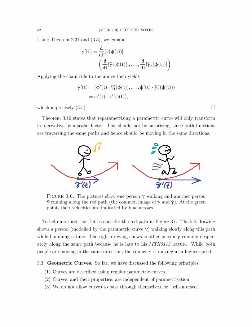
52 (MTH5113) LECTURE NOTES
Using Theorem 2.37 and (3.3), we expand
γ ′(t) =d
dt[γ(ϕ(t))]
=
(d
dt[γ1(ϕ(t))], . . . ,
d
dt[γn(ϕ(t))]
)Applying the chain rule to the above then yields
γ ′(t) = (ϕ ′(t) · γ ′1(ϕ(t)), . . . , ϕ
′(t) · γ ′n(ϕ(t)))
= ϕ ′(t) · γ ′(ϕ(t)),
which is precisely (3.5). □
Theorem 3.16 states that reparametrising a parametric curve will only transformits derivative by a scalar factor. This should not be surprising, since both functionsare traversing the same paths and hence should be moving in the same directions.
Figure 3.6. The pictures show one person γ walking and another personγ running along the red path (the common image of γ and γ). At the greenpoint, their velocities are indicated by blue arrows.
To help interpret this, let us consider the red path in Figure 3.6. The left drawingshows a person (modelled by the parametric curve γ) walking slowly along this pathwhile humming a tune. The right drawing shows another person γ running desper-ately along the same path because he is late to his MTH5113 lecture. While bothpeople are moving in the same direction, the runner γ is moving at a higher speed.
3.3. Geometric Curves. So far, we have discussed the following principles:
(1) Curves are described using regular parametric curves.(2) Curves, and their properties, are independent of parametrisation.(3) We do not allow curves to pass through themselves, or “self-intersect”.

(MTH5113) LECTURE NOTES 53
With these ideas in mind, we can now formulate a precise definition of curves:
Definition 3.17. C ⊆ Rn is called a (smooth) curve iff for any p ∈ C, there exist• An open subset V ⊆ Rn such that p ∈ V , and• A regular and injective parametric curve γ : I → C,
such that the following conditions hold:• γ is a bijection between I and C ∩ V .• The inverse γ−1 : C ∩ V → I of γ is also continuous.
Definition 3.17 draws upon some unfamiliar background from topology. For thatreason, we will not focus on the precise definition in this module. However, we are inposition to explore how Definition 3.17 relates to the above three principles.
Suppose C ⊆ Rn is a curve, as described in Definition 3.17. Then, given p ∈ C, theparametric curve γ from Definition 3.17 provides a smooth one-to-one correspondencebetween points on the interval I and points of C near p (namely, in the subset C∩V).This is illustrated in the left drawing of Figure 3.7; the open subset V is drawn inpurple, while both I and C ∩ V are coloured red.
The interpretation is that near p, the curve C looks like a “deformed” version of I(think of a bent piece of wire), while γ describes how I was deformed.
Figure 3.7. In the left drawing, a curve C is locally represented by a regu-lar, injective parametric curve γ (indicated in red), as described in Definition3.17. On the right, we have two parametric curves γ1 (in red) and γ2 (inblue) describing two parts of C. Moreover, at points where γ1 and γ2 overlap(drawn in purple), they are reparametrisations of each other.
Thus, C can be viewed as the object obtained by “gluing together” one or more“deformed intervals”. In other words, using a collection of regular parametric curves,
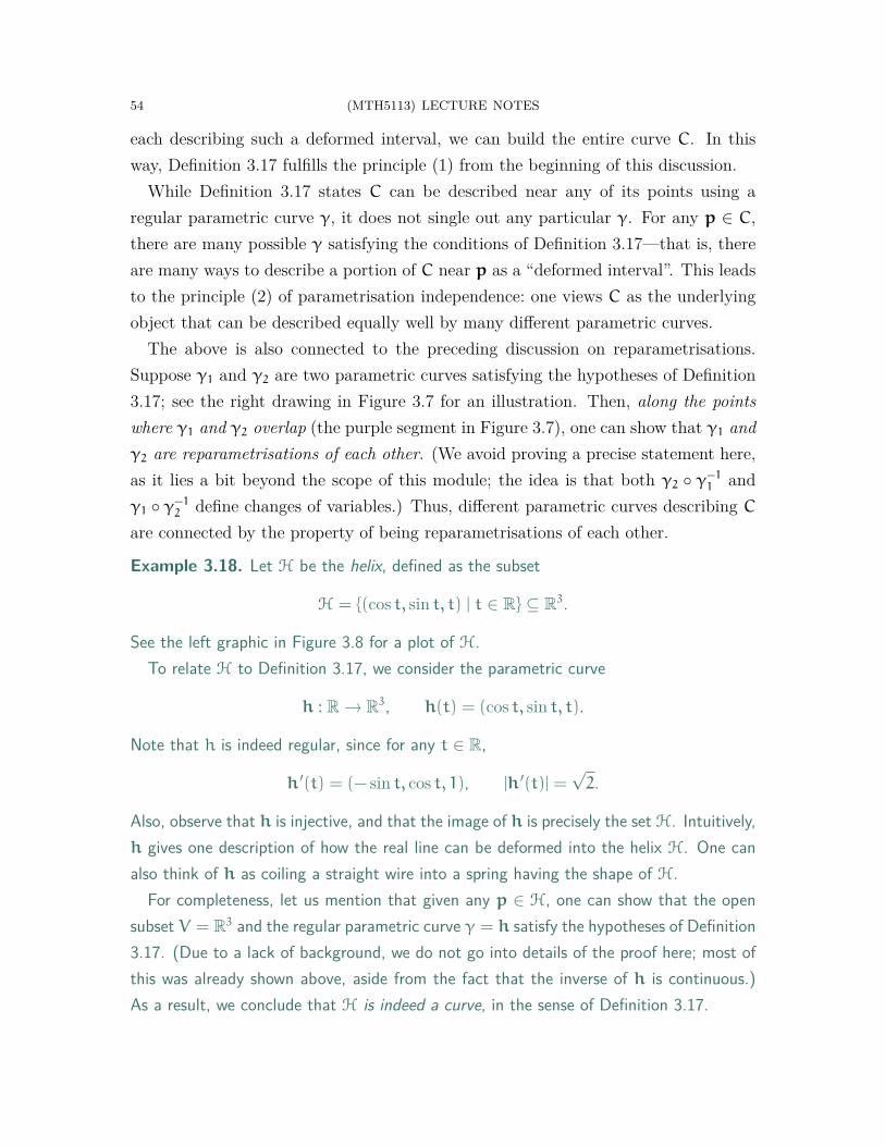
54 (MTH5113) LECTURE NOTES
each describing such a deformed interval, we can build the entire curve C. In thisway, Definition 3.17 fulfills the principle (1) from the beginning of this discussion.
While Definition 3.17 states C can be described near any of its points using aregular parametric curve γ, it does not single out any particular γ. For any p ∈ C,there are many possible γ satisfying the conditions of Definition 3.17—that is, thereare many ways to describe a portion of C near p as a “deformed interval”. This leadsto the principle (2) of parametrisation independence: one views C as the underlyingobject that can be described equally well by many different parametric curves.
The above is also connected to the preceding discussion on reparametrisations.Suppose γ1 and γ2 are two parametric curves satisfying the hypotheses of Definition3.17; see the right drawing in Figure 3.7 for an illustration. Then, along the pointswhere γ1 and γ2 overlap (the purple segment in Figure 3.7), one can show that γ1 andγ2 are reparametrisations of each other. (We avoid proving a precise statement here,as it lies a bit beyond the scope of this module; the idea is that both γ2 ◦ γ−1
1 andγ1 ◦ γ−1
2 define changes of variables.) Thus, different parametric curves describing C
are connected by the property of being reparametrisations of each other.
Example 3.18. Let H be the helix, defined as the subset
H = {(cos t, sin t, t) | t ∈ R} ⊆ R3.
See the left graphic in Figure 3.8 for a plot of H.To relate H to Definition 3.17, we consider the parametric curve
h : R → R3, h(t) = (cos t, sin t, t).
Note that h is indeed regular, since for any t ∈ R,
h ′(t) = (− sin t, cos t, 1), |h ′(t)| =√2.
Also, observe that h is injective, and that the image of h is precisely the set H. Intuitively,h gives one description of how the real line can be deformed into the helix H. One canalso think of h as coiling a straight wire into a spring having the shape of H.
For completeness, let us mention that given any p ∈ H, one can show that the opensubset V = R3 and the regular parametric curve γ = h satisfy the hypotheses of Definition3.17. (Due to a lack of background, we do not go into details of the proof here; most ofthis was already shown above, aside from the fact that the inverse of h is continuous.)As a result, we conclude that H is indeed a curve, in the sense of Definition 3.17.
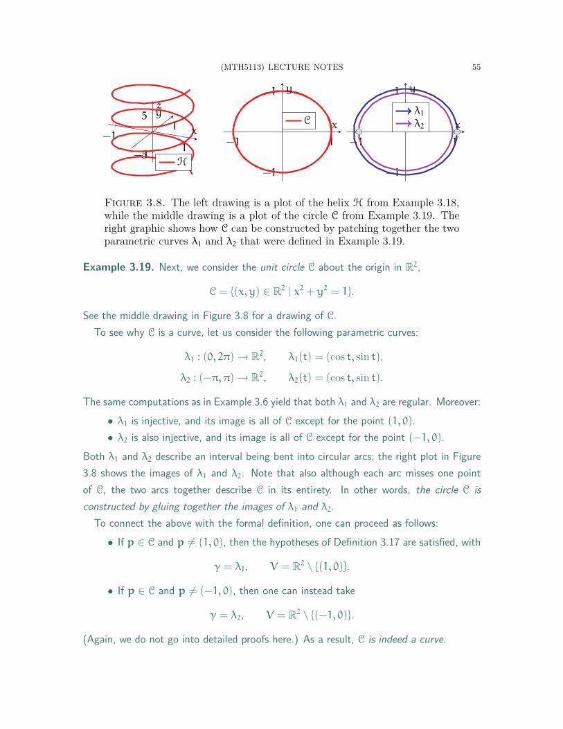
(MTH5113) LECTURE NOTES 55
−11
−1
1
−5
5
x
yz
H
−1 1
−1
1
x
y
C
−1 1
−1
1
x
y
λ1
λ2
Figure 3.8. The left drawing is a plot of the helix H from Example 3.18,while the middle drawing is a plot of the circle C from Example 3.19. Theright graphic shows how C can be constructed by patching together the twoparametric curves λ1 and λ2 that were defined in Example 3.19.
Example 3.19. Next, we consider the unit circle C about the origin in R2,
C = {(x, y) ∈ R2 | x2 + y2 = 1}.
See the middle drawing in Figure 3.8 for a drawing of C.To see why C is a curve, let us consider the following parametric curves:
λ1 : (0, 2π) → R2, λ1(t) = (cos t, sin t),
λ2 : (−π, π) → R2, λ2(t) = (cos t, sin t).
The same computations as in Example 3.6 yield that both λ1 and λ2 are regular. Moreover:• λ1 is injective, and its image is all of C except for the point (1, 0).• λ2 is also injective, and its image is all of C except for the point (−1, 0).
Both λ1 and λ2 describe an interval being bent into circular arcs; the right plot in Figure3.8 shows the images of λ1 and λ2. Note that also although each arc misses one pointof C, the two arcs together describe C in its entirety. In other words, the circle C isconstructed by gluing together the images of λ1 and λ2.
To connect the above with the formal definition, one can proceed as follows:• If p ∈ C and p 6= (1, 0), then the hypotheses of Definition 3.17 are satisfied, with
γ = λ1, V = R2 \ {(1, 0)}.
• If p ∈ C and p 6= (−1, 0), then one can instead take
γ = λ2, V = R2 \ {(−1, 0)}.
(Again, we do not go into detailed proofs here.) As a result, C is indeed a curve.
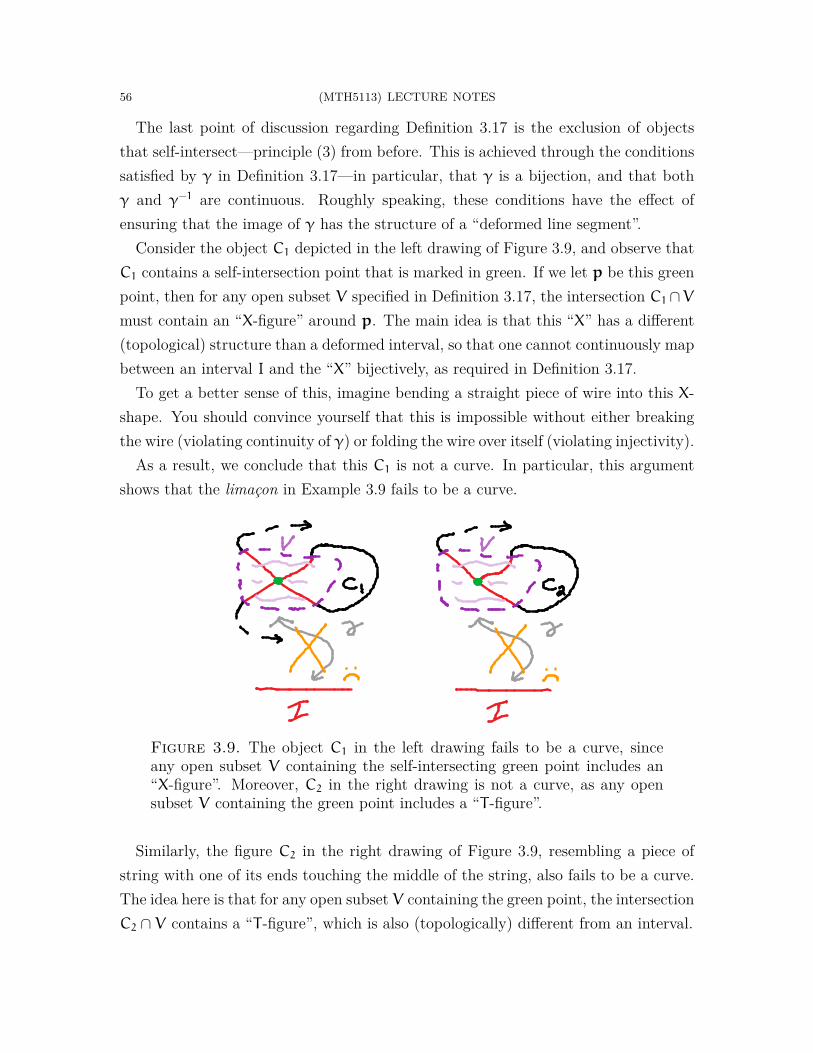
56 (MTH5113) LECTURE NOTES
The last point of discussion regarding Definition 3.17 is the exclusion of objectsthat self-intersect—principle (3) from before. This is achieved through the conditionssatisfied by γ in Definition 3.17—in particular, that γ is a bijection, and that bothγ and γ−1 are continuous. Roughly speaking, these conditions have the effect ofensuring that the image of γ has the structure of a “deformed line segment”.
Consider the object C1 depicted in the left drawing of Figure 3.9, and observe thatC1 contains a self-intersection point that is marked in green. If we let p be this greenpoint, then for any open subset V specified in Definition 3.17, the intersection C1∩V
must contain an “X-figure” around p. The main idea is that this “X” has a different(topological) structure than a deformed interval, so that one cannot continuously mapbetween an interval I and the “X” bijectively, as required in Definition 3.17.
To get a better sense of this, imagine bending a straight piece of wire into this X-shape. You should convince yourself that this is impossible without either breakingthe wire (violating continuity of γ) or folding the wire over itself (violating injectivity).
As a result, we conclude that this C1 is not a curve. In particular, this argumentshows that the limaçon in Example 3.9 fails to be a curve.
Figure 3.9. The object C1 in the left drawing fails to be a curve, sinceany open subset V containing the self-intersecting green point includes an“X-figure”. Moreover, C2 in the right drawing is not a curve, as any opensubset V containing the green point includes a “T -figure”.
Similarly, the figure C2 in the right drawing of Figure 3.9, resembling a piece ofstring with one of its ends touching the middle of the string, also fails to be a curve.The idea here is that for any open subset V containing the green point, the intersectionC2 ∩ V contains a “T -figure”, which is also (topologically) different from an interval.
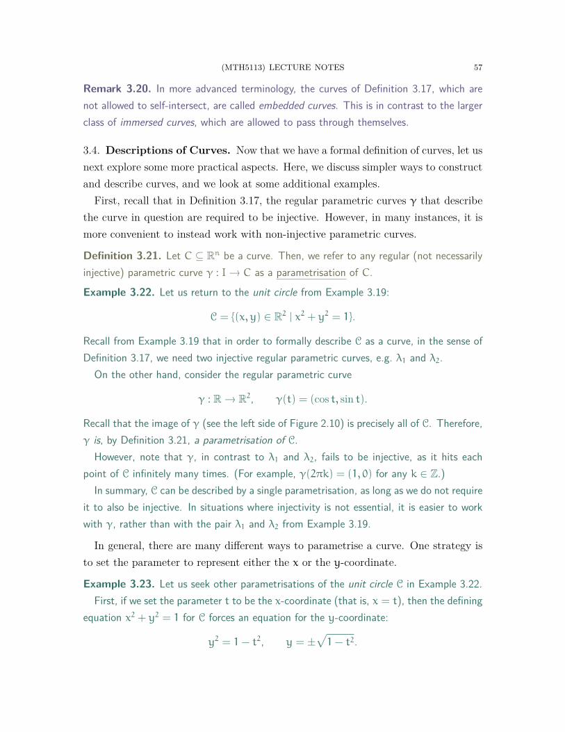
(MTH5113) LECTURE NOTES 57
Remark 3.20. In more advanced terminology, the curves of Definition 3.17, which arenot allowed to self-intersect, are called embedded curves. This is in contrast to the largerclass of immersed curves, which are allowed to pass through themselves.
3.4. Descriptions of Curves. Now that we have a formal definition of curves, let usnext explore some more practical aspects. Here, we discuss simpler ways to constructand describe curves, and we look at some additional examples.
First, recall that in Definition 3.17, the regular parametric curves γ that describethe curve in question are required to be injective. However, in many instances, it ismore convenient to instead work with non-injective parametric curves.
Definition 3.21. Let C ⊆ Rn be a curve. Then, we refer to any regular (not necessarilyinjective) parametric curve γ : I → C as a parametrisation of C.Example 3.22. Let us return to the unit circle from Example 3.19:
C = {(x, y) ∈ R2 | x2 + y2 = 1}.
Recall from Example 3.19 that in order to formally describe C as a curve, in the sense ofDefinition 3.17, we need two injective regular parametric curves, e.g. λ1 and λ2.
On the other hand, consider the regular parametric curve
γ : R → R2, γ(t) = (cos t, sin t).
Recall that the image of γ (see the left side of Figure 2.10) is precisely all of C. Therefore,γ is, by Definition 3.21, a parametrisation of C.
However, note that γ, in contrast to λ1 and λ2, fails to be injective, as it hits eachpoint of C infinitely many times. (For example, γ(2πk) = (1, 0) for any k ∈ Z.)
In summary, C can be described by a single parametrisation, as long as we do not requireit to also be injective. In situations where injectivity is not essential, it is easier to workwith γ, rather than with the pair λ1 and λ2 from Example 3.19.
In general, there are many different ways to parametrise a curve. One strategy isto set the parameter to represent either the x or the y-coordinate.
Example 3.23. Let us seek other parametrisations of the unit circle C in Example 3.22.First, if we set the parameter t to be the x-coordinate (that is, x = t), then the defining
equation x2 + y2 = 1 for C forces an equation for the y-coordinate:
y2 = 1− t2, y = ±√
1− t2.
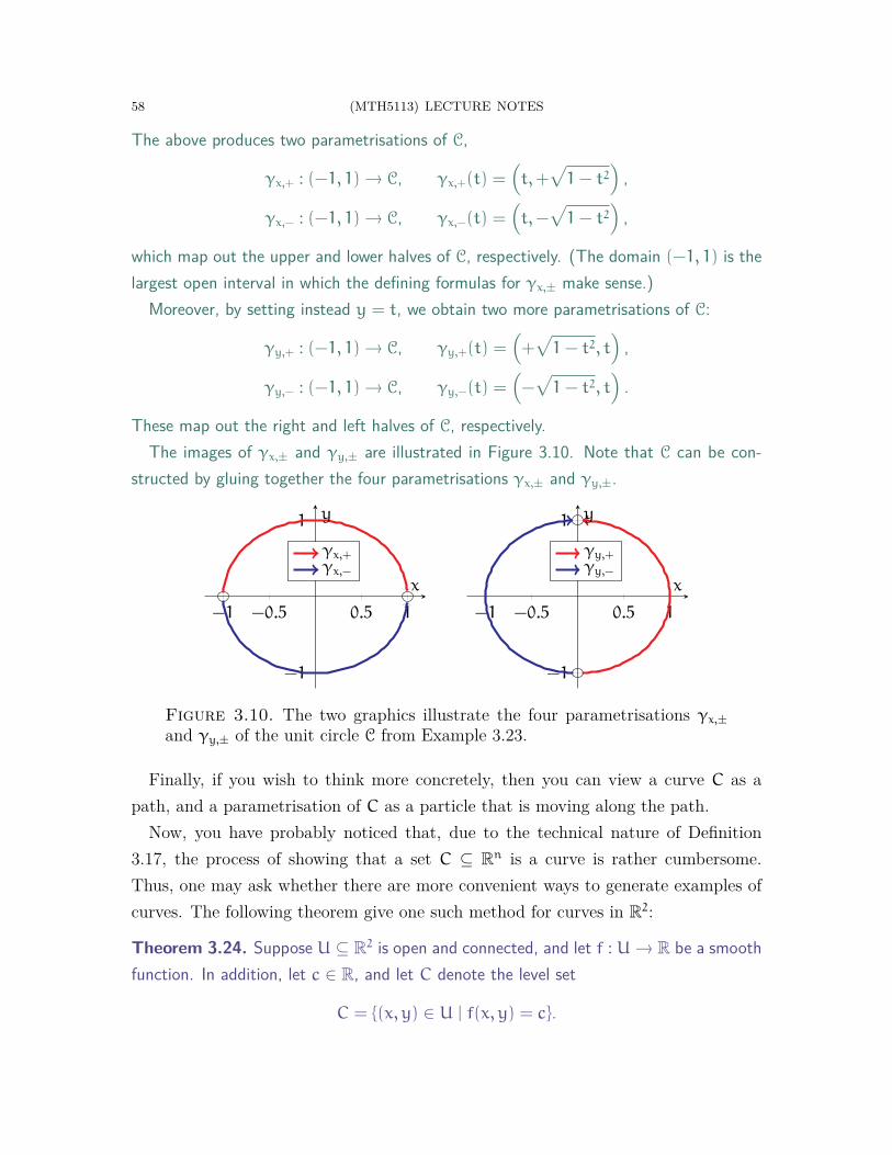
58 (MTH5113) LECTURE NOTES
The above produces two parametrisations of C,
γx,+ : (−1, 1) → C, γx,+(t) =(t,+
√1− t2
),
γx,− : (−1, 1) → C, γx,−(t) =(t,−
√1− t2
),
which map out the upper and lower halves of C, respectively. (The domain (−1, 1) is thelargest open interval in which the defining formulas for γx,± make sense.)
Moreover, by setting instead y = t, we obtain two more parametrisations of C:
γy,+ : (−1, 1) → C, γy,+(t) =(+√
1− t2, t)
,
γy,− : (−1, 1) → C, γy,−(t) =(−√
1− t2, t)
.
These map out the right and left halves of C, respectively.The images of γx,± and γy,± are illustrated in Figure 3.10. Note that C can be con-
structed by gluing together the four parametrisations γx,± and γy,±.
−1 −0.5 0.5 1
−1
1
x
y
γx,+γx,−
−1 −0.5 0.5 1
−1
1
x
y
γy,+γy,−
Figure 3.10. The two graphics illustrate the four parametrisations γx,±and γy,± of the unit circle C from Example 3.23.
Finally, if you wish to think more concretely, then you can view a curve C as apath, and a parametrisation of C as a particle that is moving along the path.
Now, you have probably noticed that, due to the technical nature of Definition3.17, the process of showing that a set C ⊆ Rn is a curve is rather cumbersome.Thus, one may ask whether there are more convenient ways to generate examples ofcurves. The following theorem give one such method for curves in R2:
Theorem 3.24. Suppose U ⊆ R2 is open and connected, and let f : U → R be a smoothfunction. In addition, let c ∈ R, and let C denote the level set
C = {(x, y) ∈ U | f(x, y) = c}.
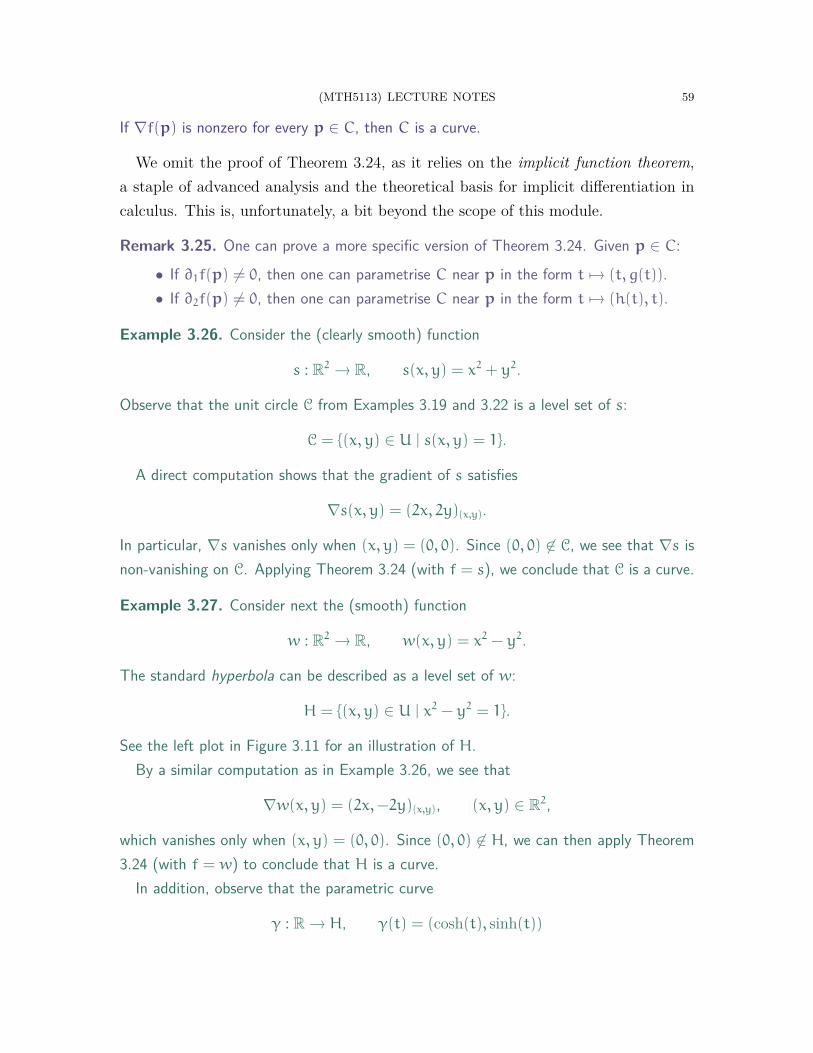
(MTH5113) LECTURE NOTES 59
If ∇f(p) is nonzero for every p ∈ C, then C is a curve.
We omit the proof of Theorem 3.24, as it relies on the implicit function theorem,a staple of advanced analysis and the theoretical basis for implicit differentiation incalculus. This is, unfortunately, a bit beyond the scope of this module.
Remark 3.25. One can prove a more specific version of Theorem 3.24. Given p ∈ C:• If ∂1f(p) 6= 0, then one can parametrise C near p in the form t 7→ (t, g(t)).• If ∂2f(p) 6= 0, then one can parametrise C near p in the form t 7→ (h(t), t).
Example 3.26. Consider the (clearly smooth) function
s : R2 → R, s(x, y) = x2 + y2.
Observe that the unit circle C from Examples 3.19 and 3.22 is a level set of s:
C = {(x, y) ∈ U | s(x, y) = 1}.
A direct computation shows that the gradient of s satisfies
∇s(x, y) = (2x, 2y)(x,y).
In particular, ∇s vanishes only when (x, y) = (0, 0). Since (0, 0) 6∈ C, we see that ∇s isnon-vanishing on C. Applying Theorem 3.24 (with f = s), we conclude that C is a curve.
Example 3.27. Consider next the (smooth) function
w : R2 → R, w(x, y) = x2 − y2.
The standard hyperbola can be described as a level set of w:
H = {(x, y) ∈ U | x2 − y2 = 1}.
See the left plot in Figure 3.11 for an illustration of H.By a similar computation as in Example 3.26, we see that
∇w(x, y) = (2x,−2y)(x,y), (x, y) ∈ R2,
which vanishes only when (x, y) = (0, 0). Since (0, 0) 6∈ H, we can then apply Theorem3.24 (with f = w) to conclude that H is a curve.
In addition, observe that the parametric curve
γ : R → H, γ(t) = (cosh(t), sinh(t))
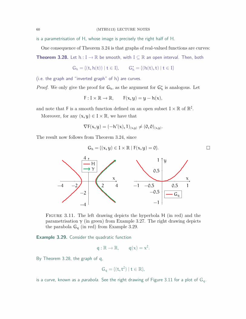
60 (MTH5113) LECTURE NOTES
is a parametrisation of H, whose image is precisely the right half of H.
One consequence of Theorem 3.24 is that graphs of real-valued functions are curves:
Theorem 3.28. Let h : I → R be smooth, with I ⊆ R an open interval. Then, both
Gh = {(t, h(t)) | t ∈ I}, G∗h = {(h(t), t) | t ∈ I}
(i.e. the graph and “inverted graph” of h) are curves.
Proof. We only give the proof for Gh, as the argument for G∗h is analogous. Let
F : I× R → R, F(x, y) = y− h(x),
and note that F is a smooth function defined on an open subset I× R of R2.Moreover, for any (x, y) ∈ I× R, we have that
∇F(x, y) = (−h ′(x), 1)(x,y) 6= (0, 0)(x,y).
The result now follows from Theorem 3.24, since
Gh = {(x, y) ∈ I× R | F(x, y) = 0}. □
−4 −2 2 4
−4
−2
2
4
x
Hγ
−1 −0.5 0.5 1
−1
−0.5
0.5
1
x
y
Gq
Figure 3.11. The left drawing depicts the hyperbola H (in red) and theparametrisation γ (in green) from Example 3.27. The right drawing depictsthe parabola Gq (in red) from Example 3.29.
Example 3.29. Consider the quadratic function
q : R → R, q(x) = x2.
By Theorem 3.28, the graph of q,
Gq = {(t, t2) | t ∈ R},
is a curve, known as a parabola. See the right drawing of Figure 3.11 for a plot of Gq.

(MTH5113) LECTURE NOTES 61
3.5. Tangent Lines. The remainder of this chapter is dedicated to exploring geo-metric properties of curves. In practice, rather than study curves directly, we oftenmeasure properties of their parametrisations, which describe the points of the curvein a way that allows us to do calculus. But, this yields another problem: does a givenparametric property actually reflect the geometry of the underlying curve?
For example, consider a curve C ⊆ Rn, which one can think of as representing apath. Also, let γ : I → Rn be a parametrisation of C, modelling a person movingalong this path. Then, the derivative γ ′(t) at any t ∈ I is certainly a property of γ,representing the person’s velocity at a certain point of C.
Note, however, that this velocity carries information beyond the properties of thepath itself. In other words, if you were given only the curve C, but not the particulartrajectory γ, then you could not recover the information given by γ ′(t). (In particular,another person running along C could have a rather different velocity.)
Therefore, for something to be a geometric property of C:
• One should be able to extract this value using a parametrisation of C.• One should obtain the same value from any parametrisation of C.
In other words, a geometric property of C must be independent of parametrisation.Now, while the derivative of γ does not give a geometric property of C, we can,
however, use this information to describe a property that is geometric in nature. Inorder to properly describe this, we first define the following:
Definition 3.30. Let γ : I → Rn be a regular parametric curve, and let t0 ∈ I. Wedefine the tangent line to γ at t0 to be the following subspace (of tangent vectors):
(3.6) Tγ(t0) ={s · γ ′(t0)γ(t0)
∣∣s ∈ R}⊆ Tγ(t0)R
n.
Remark 3.31. Note Tγ(t0) is a vector subspace of Tγ(t0)Rn, in the sense that you learnedin linear algebra, since Tγ(t0) is the span of the tangent vector γ ′(t0)γ(t0).
Let us now make some sense of Definition 3.30. Recall that γ ′(t0)γ(t0) representsthe arrow starting at the point γ(t0) on γ, and pointing in the direction γ ′(t0) alongγ. Thus, the arrows in Tγ(t0), which are all the dilations of γ ′(t0)γ(t0), trace out aline that is tangent to γ at γ(t0). This intuition justifies the name “tangent line”.
Example 3.32. Consider the parametric unit circle,
γ : R → R2, γ(t) = (cos t, sin t).

62 (MTH5113) LECTURE NOTES
At t0 = π4, we compute
γ(π4
)=
(1√2,1√2
), γ ′
(π4
)=
(−
1√2,1√2
).
By Definition 3.30, the tangent line to γ at π4
is then given by
Tγ
(π4
)=
{s · γ ′
(π4
)γ(π
4 )
∣∣∣s ∈ R}
=
{s ·(−
1√2,1√2
)(1√2, 1√
2
)∣∣∣∣s ∈ R}
.
Graphical representations of Tγ(π4) are given in Figure 3.12. In the left illustration,
the tangent vector γ ′(π4)γ(π
4) is drawn in blue. The arrows in the middle picture depict
some other elements of Tγ(π4 ). Lastly, in the right illustration, the tangent line Tγ(π4) is
represented as a purple line, which is traced out by all the arrows in Tγ(π4).
−2 −1 1 2
−2
−1
1
2
x
y γ
−2 −1 1 2
−2
−1
1
2
x
y γ
−2 −1 1 2
−2
−1
1
2
x
y γ
Tγ(π4)
Figure 3.12. The pictures show the setup from Example 3.32. In the firstplot, the blue arrow shows the tangent vector γ ′(π
4)γ(π
4). The middle plot
contains some additional elements of Tγ(π4 ), drawn as coloured arrows. Inthe right plot, the tangent line Tγ(
π4) is represented as a purple line.
Example 3.33. Let f : (−1, 1) → R be smooth, and consider the parametric curve
γf : (−1, 1) → R2, γf(t) = (t, f(t)),
whose image is the graph of f. Then, for any t ∈ (−1, 1), we have that
γ ′f(t) = (1, f ′(t)),
hence the tangent line of γf at t is
Tγf(t) =
{s · (1, f ′(t))(t,f(t))
∣∣s ∈ R}
.
Next, we show how these tangent lines define a geometric property of curves.

(MTH5113) LECTURE NOTES 63
Theorem 3.34. Let γ : I → Rn and γ : I → Rn be regular parametric curves, and let γbe a reparametrisation of γ, with change of variables ϕ : I → I. Then, for any t ∈ I,
(3.7) Tγ(t) = Tγ(ϕ(t)).
Recall, in the setting of Theorem 3.34, that γ(t) and γ(ϕ(t)) refer to the samepoint. Thus, the formula (3.7) can be interpreted as follows: at common points alongthe trajectories of γ and γ, one obtains identical tangent lines for both γ and γ.
Proof of Theorem 3.34. Let us abbreviate t = ϕ(t). Then, Theorem 3.16 yields
γ ′(t)γ(t) =1
ϕ ′(t)· γ ′(t)γ(t), t ∈ I.
Using Definition 3.30, we conclude that
Tγ(t) ={s · γ ′(t)γ(t)
∣∣s ∈ R}
={s · γ ′(t)γ(t)
∣∣s ∈ R}
= Tγ(t),
since every scalar multiple of γ ′(t)γ(t) is a multiple of γ ′(t)γ(t), and vice versa. □
Though a parametric curve’s speed can change after reparametrising, it will alwayspoint in one of two (opposite) directions. Thus, by taking all scalar multiples of thetangent vector, (3.6) precisely factors out all information about speed while preservingthe directional information that is independent of parametrisation.
Using Theorem 3.34, we can now formally define a geometric property:
Definition 3.35. The tangent line to a curve C ⊆ Rn at a point p ∈ C is defined as
(3.8) TpC = Tγ(t0),
where γ : I → C is any parametrisation of C, and where t0 ∈ I satisfies γ(t0) = p.
In particular, a tangent line to C is obtained by computing the correspondingtangent line to any parametrisation of C. Indeed, Theorem 3.34 guarantees that wewill always obtain the same answer regardless of our choice of parametrisation.
Example 3.36. Consider the helix H from Example 3.18 (see also Figure 3.8). Recallfrom Example 3.18 that the following function is a parametrisation of H:
h : R → H, h(t) = (cos t, sin t, t).
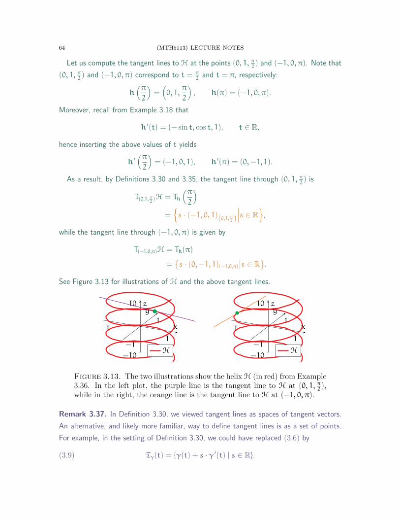
64 (MTH5113) LECTURE NOTES
Let us compute the tangent lines to H at the points (0, 1, π2) and (−1, 0, π). Note that
(0, 1, π2) and (−1, 0, π) correspond to t = π
2and t = π, respectively:
h(π2
)=(0, 1,
π
2
), h(π) = (−1, 0, π).
Moreover, recall from Example 3.18 that
h ′(t) = (− sin t, cos t, 1), t ∈ R,
hence inserting the above values of t yields
h ′(π2
)= (−1, 0, 1), h ′(π) = (0,−1, 1).
As a result, by Definitions 3.30 and 3.35, the tangent line through (0, 1, π2) is
T(0,1,π2)H = Th
(π2
)=
{s · (−1, 0, 1)(0,1,π2 )
∣∣∣s ∈ R}
,
while the tangent line through (−1, 0, π) is given by
T(−1,0,π)H = Th(π)
={s · (0,−1, 1)(−1,0,π)
∣∣s ∈ R}
.
See Figure 3.13 for illustrations of H and the above tangent lines.
−1
1−1
1
−10
10
x
yz
H
−1
1−1
1
−10
10
x
yz
H
Figure 3.13. The two illustrations show the helix H (in red) from Example3.36. In the left plot, the purple line is the tangent line to H at (0, 1, π
2),
while in the right, the orange line is the tangent line to H at (−1, 0, π).
Remark 3.37. In Definition 3.30, we viewed tangent lines as spaces of tangent vectors.An alternative, and likely more familiar, way to define tangent lines is as a set of points.For example, in the setting of Definition 3.30, we could have replaced (3.6) by
(3.9) Tγ(t) = {γ(t) + s · γ ′(t) | s ∈ R}.
(MTH5113) LECTURE NOTES 65
Observe that the right-hand side of (3.9) is simply the image of the parametric line thatpasses through γ(t) and that is aligned in the direction of γ ′(t).
The definition (3.9) has the advantage of being more straightforward; in fact, you mayhave already encountered this in your calculus modules. Moreover, the set Tγ(t) coincideswith the purple and orange lines drawn in Figures 3.12 and 3.13.
On the other hand, the more modern Definitions 3.30 and 3.35 characterise tangentlines as a set of directions along a curve, an intuition that will be quite useful in the future.Furthermore, (3.6) highlights the linear structure that is inherent to the tangent line. Inparticular, the set Tγ(t0) is a 1-dimensional vector space (see Remark 3.31), whereas theset Tγ(t0) in (3.9) has no such connection to linear algebra. For these reasons, we adoptDefinitions 3.30 and 3.35 as our formal starting points for discussions.
3.6. Tangents and Normals. As before, let C ⊆ Rn be a curve, and consider apoint p ∈ C. We noted that the tangent line TpC is a 1-dimensional vector space andhence has the same structure as the real line. Thus, there are exactly two elementst±p ∈ TpC having unit length, which are pointing in opposite directions.
This above observation leads us to the following definition:
Definition 3.38. Let C ⊆ Rn be a curve, and let p ∈ C. We define the unit tangentsto C at p to be the two elements t±p of TpC such that |t±p | = 1.
Example 3.39. Consider the y-axis in R3,
Ly = {(0, t, 0) | t ∈ R}.
One can show (though we omit this detail here) that Ly is a curve in R3. Let us now findthe unit tangents to Ly at the point p = (0,−1, 0) ∈ Ly.
The first step is compute the tangent line to Ly at p. For this, note that
ℓ : R → R3, ℓ(t) = (0, t, 0)
is a parametrisation of Ly, and that
ℓ(−1) = (0,−1, 0), ℓ ′(−1) = (0, 1, 0).
As a result, we see from Definitions 3.30 and 3.35 that
TpLy = Tℓ(−1)
= {(0, s, 0)(0,−1,0) | s ∈ R}.

66 (MTH5113) LECTURE NOTES
By Definition 3.38, the unit tangents to Ly at (0,−1, 0) are the two elements of TpLy
with unit length. Clearly, these are given by the tangent vectors
t±(0,−1,0) = (0,±1, 0)(0,−1,0).
See the left plot in Figure 3.14 for an illustration of the above—the two unit tangents toLy at p are depicted as purple and blue arrows.
−2−1
12
−2
2
−2
2
x
y
z
Ly
−2 −1 1 2
−2
−1
1
2
x
y C
TpC
Figure 3.14. The graphics contain the settings of Examples 3.39 (left)and 3.42 (right). Furthermore, in both plots, the unit tangents at the givenpoints p are drawn as purple and blue arrows.
Let us now return to the general curve C ⊆ Rn and point p ∈ C. Recall (seeFigures 3.12 and 3.13) that TpC can be represented as a line in Rn that intersects C
at p, as well as points along the directions of C at p. As a result, the unit tangentsto C at p, which point in opposite directions along this line, correspond to the twodirections that one can go along C from the point p.
To be more concrete, consider the right plot in Figure 3.14, illustrating the casewhere C is a circle in R2, and where p is the green point. Here, the purple and bluearrows, representing unit tangents t±p to C at p, point in opposite tangent directionsalong C. In particular, the purple arrow captures the anticlockwise direction alongC, while the blue arrow corresponds to the clockwise direction.
Remark 3.40. The above also suggests another interpretation for TpC itself. Since TpC
consists of all scalar multiples of the unit tangents t±p , it follows that TpC is a combinationof all the directions and speeds that one could move along C at p. In other words, TpCrepresents all the possible velocities one could have at p while moving along C.
Since we often work with curves through their parametrisations, it will be conve-nient to have a parametric formula for computing unit tangents:

(MTH5113) LECTURE NOTES 67
Theorem 3.41. Let C ⊆ Rn be a curve, let γ : I → C be a parametrisation of C, andlet t0 ∈ I. Then, the unit tangents to C at the point p = γ(t0) are given by
(3.10) ± |γ ′(t0)|−1 · γ ′(t0)γ(t0).
Proof. The tangent vectors t±p = ±|γ ′(t0)|−1 · γ ′(t0)γ(tp) lie in TpC by definition and
clearly have unit length, thus they are unit tangents to C at p. □
Example 3.42. Next, let C be the unit circle from Example 3.19. Recall, from Example3.22, that the following function is a parametrisation of C:
γ : R → R2, γ(t) = (cos t, sin t)
Let us find the unit tangents to C at the point
p =
(1√2,1√2
)= γ
(π4
).
For this, we simply apply Theorem 3.41 using the above γ (with t0 =π4) to obtain
±∣∣∣γ ′(π4
)∣∣∣−1
· γ ′(π4
)γ(π
4)= ±1 ·
(−
1√2,1√2
)(
1√2, 1√
2
)= ±
(−
1√2,1√2
)(
1√2, 1√
2
).
See the right plot of Figure 3.14; the unit tangents are drawn in purple and blue.
Next, we restrict our attention only to the case n = 2. Given a curve C ⊆ R2 andp ∈ C, the tangent line TpC can be viewed as a line sitting within a 2-dimensionalplane. More formally, TpC is a 1-dimensional subspace of the 2-dimensional vectorspace TpR2. Thus, there is one remaining dimension in TpR2 perpendicular to TpC,capturing the directions perpendicular, or normal, to C at p.
As before, we focus on the unit vectors in these normal directions:
Definition 3.43. Let C ⊆ R2 be a curve, and let p ∈ C. Then, np ∈ TpR2 is a unitnormal to C at p iff np is perpendicular to every element of TpC and |np| = 1.
The unit normals to a curve can be obtained from the unit tangents:
Theorem 3.44. Let C ⊆ R2 be a curve, and let p ∈ C. If ±(v1, v2)p ∈ TpC are the unittangents to C at p, then the unit normals to C at p are given by
(3.11) n±p = ±(−v2, v1)p.
68 (MTH5113) LECTURE NOTES
Proof. Since (v1, v2) is a unit vector, then a direct computation shows that
±(−v2, v1)p · ±(v1, v2)p = 0, |± (−v2, v1)p| = 1,
and hence n±p are indeed unit normals to C at p. Since there is only one normal
dimension, then n±p must also be the only unit normals to C at p. □
Remark 3.45. The intuition behind (3.11) is that the direction (−v2, v1) is precisely a90 degree rotation from (v1, v2). A slick way to see this is through complex numbers—ananticlockwise rotation of the complex number v1 + iv2 by 90 degrees yields
ei·π2 (v1 + iv2) = i(v1 + iv2)
= −v2 + iv1.
Example 3.46. Consider again the circle C and the point p ∈ C from Example 3.42:
C = {(x, y) ∈ R2 | x2 + y2 = 1}, p =
(1√2,1√2
).
Recall, from Example 3.42, that unit tangents to C at p are
±(−
1√2,1√2
)(
1√2, 1√
2
).
Then, by Theorem 3.44, the unit normals to C at p are given by
±(−
1√2,−
1√2
)(
1√2, 1√
2
) = ±(
1√2,1√2
)(
1√2, 1√
2
).
These unit normals to C are illustrated (in orange and blue) in the left plot of Figure 3.15.
When the curve C is also a level set, in the sense of Theorem 3.24, there is anothermethod with which one can compute the unit normals directly:
Theorem 3.47. Assume the setting of Theorem 3.24—let C be the curve
C = {(x, y) ∈ U | f(x, y) = c},
where U ⊆ R2, c ∈ R, and f : U → R is a smooth function such that ∇f(q) is nonzerofor each q ∈ C. Then, given any p ∈ C, the unit normals to C at p are
(3.12) n±p = ±|∇f(p)|−1 · ∇f(p).
Proof. Let γ : I → C be a parametrisation of C, whose values can be expanded as
γ(t) = (x(t), y(t)), t ∈ I,
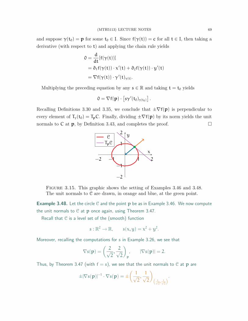
(MTH5113) LECTURE NOTES 69
and suppose γ(t0) = p for some t0 ∈ I. Since f(γ(t)) = c for all t ∈ I, then taking aderivative (with respect to t) and applying the chain rule yields
0 =d
dt[f(γ(t))]
= ∂1f(γ(t)) · x ′(t) + ∂2f(γ(t)) · y ′(t)
= ∇f(γ(t)) · γ ′(t)γ(t).
Multiplying the preceding equation by any s ∈ R and taking t = t0 yields
0 = ∇f(p) ·[sγ ′(t0)γ(t0)
].
Recalling Definitions 3.30 and 3.35, we conclude that ±∇f(p) is perpendicular toevery element of Tγ(t0) = TpC. Finally, dividing ±∇f(p) by its norm yields the unitnormals to C at p, by Definition 3.43, and completes the proof. □
−2 −1 1 2
−2
−1
1
2
x
yC
TpC
Figure 3.15. This graphic shows the setting of Examples 3.46 and 3.48.The unit normals to C are drawn, in orange and blue, at the green point.
Example 3.48. Let the circle C and the point p be as in Example 3.46. We now computethe unit normals to C at p once again, using Theorem 3.47.
Recall that C is a level set of the (smooth) function
s : R2 → R, s(x, y) = x2 + y2.
Moreover, recalling the computations for s in Example 3.26, we see that
∇s(p) =
(2√2,2√2
)p
, |∇s(p)| = 2.
Thus, by Theorem 3.47 (with f = s), we see that the unit normals to C at p are
±|∇s(p)|−1 · ∇s(p) = ±(
1√2,1√2
)(
1√2, 1√
2
).
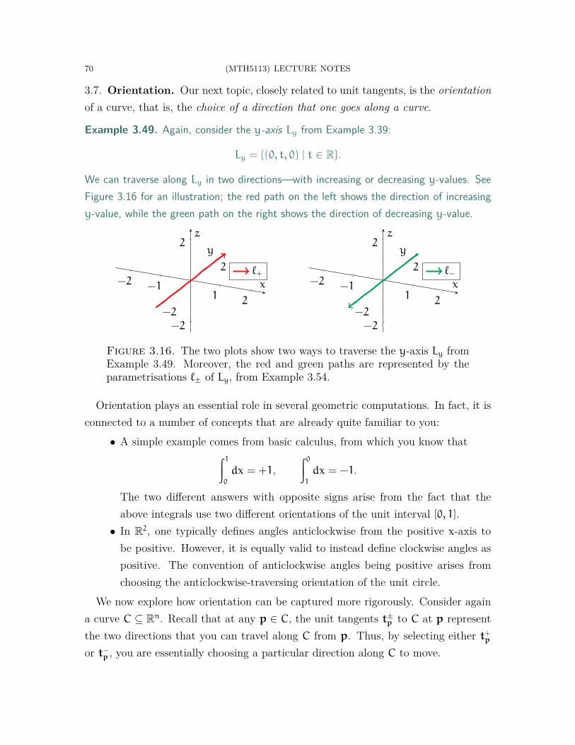
70 (MTH5113) LECTURE NOTES
3.7. Orientation. Our next topic, closely related to unit tangents, is the orientationof a curve, that is, the choice of a direction that one goes along a curve.
Example 3.49. Again, consider the y-axis Ly from Example 3.39:
Ly = {(0, t, 0) | t ∈ R}.
We can traverse along Ly in two directions—with increasing or decreasing y-values. SeeFigure 3.16 for an illustration; the red path on the left shows the direction of increasingy-value, while the green path on the right shows the direction of decreasing y-value.
−2 −11 2
−2
2
−2
2
x
y
z
ℓ+−2 −1
1 2−2
2
−2
2
x
y
z
ℓ−
Figure 3.16. The two plots show two ways to traverse the y-axis Ly fromExample 3.49. Moreover, the red and green paths are represented by theparametrisations ℓ± of Ly, from Example 3.54.
Orientation plays an essential role in several geometric computations. In fact, it isconnected to a number of concepts that are already quite familiar to you:
• A simple example comes from basic calculus, from which you know that∫ 1
0
dx = +1,∫ 0
1
dx = −1.
The two different answers with opposite signs arise from the fact that theabove integrals use two different orientations of the unit interval [0, 1].
• In R2, one typically defines angles anticlockwise from the positive x-axis tobe positive. However, it is equally valid to instead define clockwise angles aspositive. The convention of anticlockwise angles being positive arises fromchoosing the anticlockwise-traversing orientation of the unit circle.
We now explore how orientation can be captured more rigorously. Consider againa curve C ⊆ Rn. Recall that at any p ∈ C, the unit tangents t±p to C at p representthe two directions that you can travel along C from p. Thus, by selecting either t+p
or t−p , you are essentially choosing a particular direction along C to move.

(MTH5113) LECTURE NOTES 71
Now, we should keep in mind that the above selection was only for a single point.To settle on a direction along all of C, we must choose a unit tangent tq ∈ TqC ateach point q ∈ C. Furthermore, our choices of directions must be consistent with eachother, in that one cannot select one direction at some point and then suddenly jumpto the opposite direction as one slides along C.
All these considerations lead to the following definition:
Definition 3.50. An orientation of a curve C ⊆ Rn is a choice of a unit tangent tp ∈ TpC
to C at each p ∈ C, such that the tp’s vary continuously with respect to p.
Example 3.51. We can now discuss more precisely the y-axis Ly from Example 3.49:
Ly = {(0, t, 0) | t ∈ R}.
Recall (see Example 3.39) that the following is an injective parametrisation of (all of) Ly:
ℓ : R → Ly, ℓ(t) = (0, t, 0).
Moreover, at any point (0, t0, 0) ∈ Ly, we have that
ℓ(t0) = (0, t0, 0), ℓ ′(t0) = (0, 1, 0), |ℓ ′(t0)| = 1.
Thus, by Theorem 3.41, we conclude that the unit tangents to Ly at (0, t0, 0) are
±|ℓ ′(t0)|−1 · ℓ ′(t0)ℓ(t0) = (0,±1, 0)(0,t0,0).
From this, we see that one orientation of Ly can be constructed by selecting the unittangent vector (0,+1, 0)(0,t,0) at each (0, t, 0) ∈ Ly; this corresponds to the directionof increasing y-value. The remaining orientation of Ly, representing the direction ofdecreasing y-value, is captured by the choice of (0,−1, 0)(0,t,0) at each (0, t, 0) ∈ Ly.
Note one cannot jump from (0,+1, 0) to (0,−1, 0) anywhere on Ly, or vice versa, asDefinition 3.56 requires our choice of unit tangent vectors to vary continuously.
Orientations of curves can also be described using parametrisations. Roughly, aparametrisation γ : I → C of a curve C ⊆ Rn selects a direction of traversal along C.To be more precise, γ creates a natural choice of unit tangents
(3.13) + |γ ′(t)|−1 · γ ′(t)γ(t), t ∈ I,
to C (by Theorem 3.41), corresponding to the direction γ travels along C.With the above motivation, we now make the following definition:
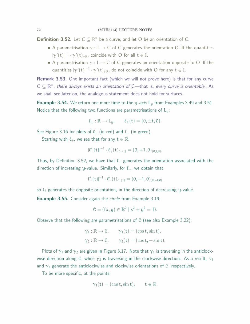
72 (MTH5113) LECTURE NOTES
Definition 3.52. Let C ⊆ Rn be a curve, and let O be an orientation of C.• A parametrisation γ : I → C of C generates the orientation O iff the quantities|γ ′(t)|−1 · γ ′(t)γ(t) coincide with O for all t ∈ I.
• A parametrisation γ : I → C of C generates an orientation opposite to O iff thequantities |γ ′(t)|−1 · γ ′(t)γ(t) do not coincide with O for any t ∈ I.
Remark 3.53. One important fact (which we will not prove here) is that for any curveC ⊆ Rn, there always exists an orientation of C—that is, every curve is orientable. Aswe shall see later on, the analogous statement does not hold for surfaces.Example 3.54. We return one more time to the y-axis Ly from Examples 3.49 and 3.51.Notice that the following two functions are parametrisations of Ly:
ℓ± : R → Ly, ℓ±(t) = (0,±t, 0).
See Figure 3.16 for plots of ℓ+ (in red) and ℓ− (in green).Starting with ℓ+, we see that for any t ∈ R,
|ℓ ′+(t)|−1 · ℓ ′+(t)ℓ+(t) = (0,+1, 0)(0,t,0).
Thus, by Definition 3.52, we have that ℓ+ generates the orientation associated with thedirection of increasing y-value. Similarly, for ℓ−, we obtain that
|ℓ ′−(t)|−1 · ℓ ′−(t)ℓ−(t) = (0,−1, 0)(0,−t,0),
so ℓ2 generates the opposite orientation, in the direction of decreasing y-value.Example 3.55. Consider again the circle from Example 3.19:
C = {(x, y) ∈ R2 | x2 + y2 = 1}.
Observe that the following are parametrisations of C (see also Example 3.22):
γ1 : R → C, γ1(t) = (cos t, sin t),
γ2 : R → C, γ2(t) = (cos t,− sin t).
Plots of γ1 and γ2 are given in Figure 3.17. Note that γ1 is traversing in the anticlock-wise direction along C, while γ2 is traversing in the clockwise direction. As a result, γ1
and γ2 generate the anticlockwise and clockwise orientations of C, respectively.To be more specific, at the points
γ1(t) = (cos t, sin t), t ∈ R,
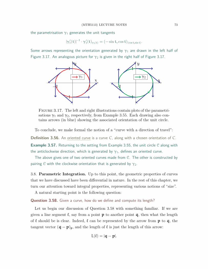
(MTH5113) LECTURE NOTES 73
the parametrisation γ1 generates the unit tangents
|γ ′1(t)|
−1 · γ ′1(t)γ1(t) = (− sin t, cos t)(cos t,sin t).
Some arrows representing the orientation generated by γ1 are drawn in the left half ofFigure 3.17. An analogous picture for γ2 is given in the right half of Figure 3.17.
−1 1
−1
1
x
y
γ1
−1 1
−1
1
x
y
γ2
Figure 3.17. The left and right illustrations contain plots of the parametri-sations γ1 and γ2, respectively, from Example 3.55. Each drawing also con-tains arrows (in blue) showing the associated orientation of the unit circle.
To conclude, we make formal the notion of a “curve with a direction of travel”:
Definition 3.56. An oriented curve is a curve C, along with a chosen orientation of C.Example 3.57. Returning to the setting from Example 3.55, the unit circle C along withthe anticlockwise direction, which is generated by γ1, defines an oriented curve.
The above gives one of two oriented curves made from C. The other is constructed bypairing C with the clockwise orientation that is generated by γ2.
3.8. Parametric Integration. Up to this point, the geometric properties of curvesthat we have discussed have been differential in nature. In the rest of this chapter, weturn our attention toward integral properties, representing various notions of “size”.
A natural starting point is the following question:
Question 3.58. Given a curve, how do we define and compute its length?
Let us begin our discussion of Question 3.58 with something familiar. If we aregiven a line segment ℓ, say from a point p to another point q, then what the lengthof ℓ should be is clear. Indeed, ℓ can be represented by the arrow from p to q, thetangent vector (q− p)p, and the length of ℓ is just the length of this arrow:
L(ℓ) = |q− p|.
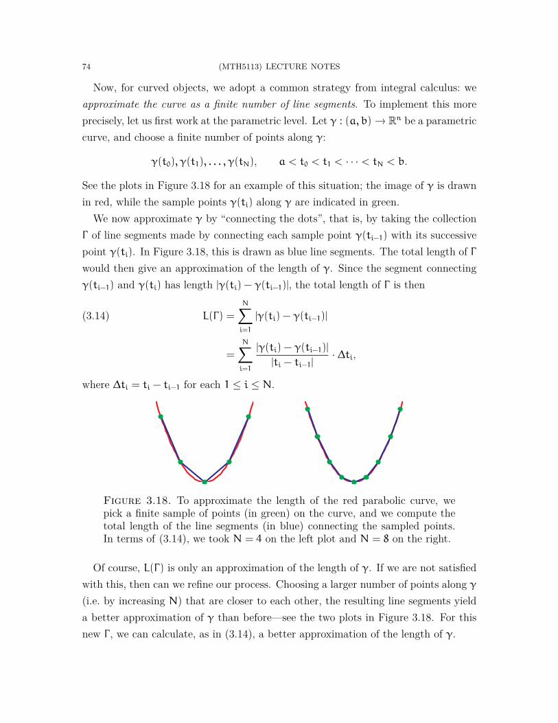
74 (MTH5113) LECTURE NOTES
Now, for curved objects, we adopt a common strategy from integral calculus: weapproximate the curve as a finite number of line segments. To implement this moreprecisely, let us first work at the parametric level. Let γ : (a, b) → Rn be a parametriccurve, and choose a finite number of points along γ:
γ(t0), γ(t1), . . . , γ(tN), a < t0 < t1 < · · · < tN < b.
See the plots in Figure 3.18 for an example of this situation; the image of γ is drawnin red, while the sample points γ(ti) along γ are indicated in green.
We now approximate γ by “connecting the dots”, that is, by taking the collectionΓ of line segments made by connecting each sample point γ(ti−1) with its successivepoint γ(ti). In Figure 3.18, this is drawn as blue line segments. The total length of Γwould then give an approximation of the length of γ. Since the segment connectingγ(ti−1) and γ(ti) has length |γ(ti) − γ(ti−1)|, the total length of Γ is then
L(Γ) =
N∑i=1
|γ(ti) − γ(ti−1)|(3.14)
=
N∑i=1
|γ(ti) − γ(ti−1)|
|ti − ti−1|· ∆ti,
where ∆ti = ti − ti−1 for each 1 ≤ i ≤ N.
Figure 3.18. To approximate the length of the red parabolic curve, wepick a finite sample of points (in green) on the curve, and we compute thetotal length of the line segments (in blue) connecting the sampled points.In terms of (3.14), we took N = 4 on the left plot and N = 8 on the right.
Of course, L(Γ) is only an approximation of the length of γ. If we are not satisfiedwith this, then can we refine our process. Choosing a larger number of points along γ
(i.e. by increasing N) that are closer to each other, the resulting line segments yielda better approximation of γ than before—see the two plots in Figure 3.18. For thisnew Γ , we can calculate, as in (3.14), a better approximation of the length of γ.
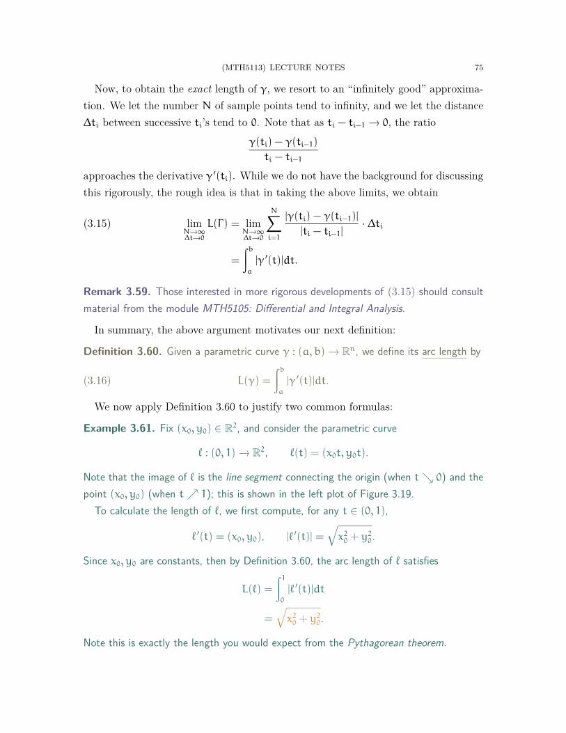
(MTH5113) LECTURE NOTES 75
Now, to obtain the exact length of γ, we resort to an “infinitely good” approxima-tion. We let the number N of sample points tend to infinity, and we let the distance∆ti between successive ti’s tend to 0. Note that as ti − ti−1 → 0, the ratio
γ(ti) − γ(ti−1)
ti − ti−1
approaches the derivative γ ′(ti). While we do not have the background for discussingthis rigorously, the rough idea is that in taking the above limits, we obtain
limN→∞∆t→0
L(Γ) = limN→∞∆t→0
N∑i=1
|γ(ti) − γ(ti−1)|
|ti − ti−1|· ∆ti(3.15)
=
∫b
a
|γ ′(t)|dt.
Remark 3.59. Those interested in more rigorous developments of (3.15) should consultmaterial from the module MTH5105: Differential and Integral Analysis.
In summary, the above argument motivates our next definition:
Definition 3.60. Given a parametric curve γ : (a, b) → Rn, we define its arc length by
(3.16) L(γ) =
∫b
a
|γ ′(t)|dt.
We now apply Definition 3.60 to justify two common formulas:
Example 3.61. Fix (x0, y0) ∈ R2, and consider the parametric curve
ℓ : (0, 1) → R2, ℓ(t) = (x0t, y0t).
Note that the image of ℓ is the line segment connecting the origin (when t ↘ 0) and thepoint (x0, y0) (when t ↗ 1); this is shown in the left plot of Figure 3.19.
To calculate the length of ℓ, we first compute, for any t ∈ (0, 1),
ℓ ′(t) = (x0, y0), |ℓ ′(t)| =√
x20 + y20.
Since x0, y0 are constants, then by Definition 3.60, the arc length of ℓ satisfies
L(ℓ) =
∫ 1
0
|ℓ ′(t)|dt
=√
x20 + y20.
Note this is exactly the length you would expect from the Pythagorean theorem.
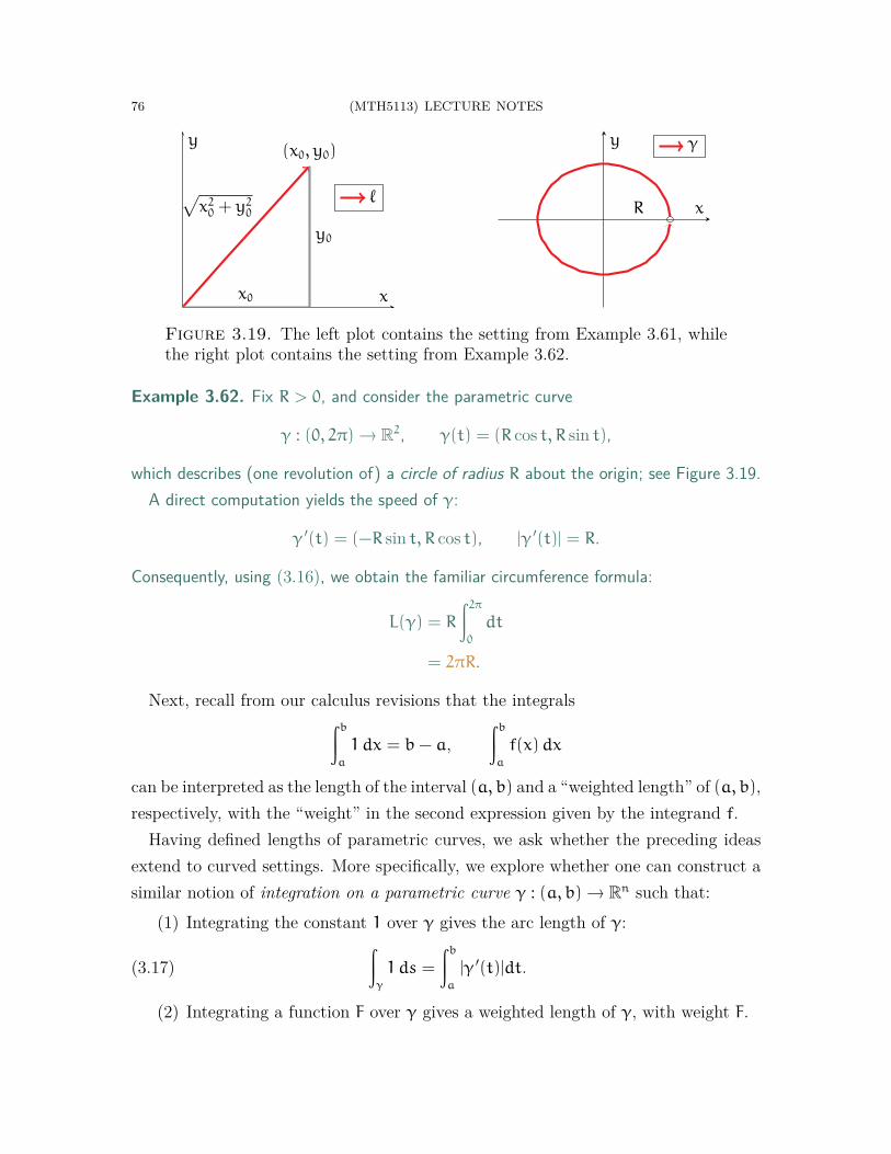
76 (MTH5113) LECTURE NOTES
(x0, y0)
y0
x0
√x20 + y2
0
x
y
ℓR x
y γ
Figure 3.19. The left plot contains the setting from Example 3.61, whilethe right plot contains the setting from Example 3.62.
Example 3.62. Fix R > 0, and consider the parametric curve
γ : (0, 2π) → R2, γ(t) = (R cos t, R sin t),
which describes (one revolution of) a circle of radius R about the origin; see Figure 3.19.A direct computation yields the speed of γ:
γ ′(t) = (−R sin t, R cos t), |γ ′(t)| = R.
Consequently, using (3.16), we obtain the familiar circumference formula:
L(γ) = R
∫ 2π
0
dt
= 2πR.
Next, recall from our calculus revisions that the integrals∫b
a
1 dx = b− a,∫b
a
f(x)dx
can be interpreted as the length of the interval (a, b) and a “weighted length” of (a, b),respectively, with the “weight” in the second expression given by the integrand f.
Having defined lengths of parametric curves, we ask whether the preceding ideasextend to curved settings. More specifically, we explore whether one can construct asimilar notion of integration on a parametric curve γ : (a, b) → Rn such that:
(1) Integrating the constant 1 over γ gives the arc length of γ:
(3.17)∫γ
1 ds =
∫b
a
|γ ′(t)|dt.
(2) Integrating a function F over γ gives a weighted length of γ, with weight F.

(MTH5113) LECTURE NOTES 77
For point (2), it makes sense, in light of the right-hand side of (3.17), to insert F
into the integrand there, as this fits with the intuition of F being a weight. Moreover,since |γ ′(t)| represents the speed of γ at γ(t), it would make sense that the weight Fis also being applied at the same point γ(t). This leads us to a formal definition:
Definition 3.63. Let γ : (a, b) → Rn be a parametric curve, and let F be a real-valuedfunction that is defined on the image of γ. We define the curve integral of F over γ by
(3.18)∫γ
F ds =
∫b
a
F(γ(t))|γ ′(t)|dt.
Remark 3.64. Curve integrals are also commonly known as path or line integrals.
−2−1
12
−2
2
−10
−5
5
10
x
y
zh∗
Figure 3.20. The above is a plot of h∗ from Example 3.65.
Example 3.65. Consider a finite portion of the parametric helix from Example 3.18:
h∗ : (−2π, 2π) → R3, h∗(t) = (cos t, sin t, t),
In particular, the image of h∗ is part a helix that revolves twice around the z-axis; seeFigure 3.20. Let us now compute the integral over h∗ of the function
G : R3 → R, G(x, y, z) = x2 + y2 + z2.
First, observe that direct computations yield
|h ′∗(t)| =
√2, G(h∗(t)) = 1+ t2.
As a result, applying Definition 3.63, we obtain∫h∗
Gds =√2
∫ 2π
−2π
(1+ t2)dt
=√2
[4π+
2
3(2π)3
].
78 (MTH5113) LECTURE NOTES
3.9. Curve Integrals. We had previously hinted that the arc length is a geometricproperty of curves. However, we have yet to justify this statement. To see why thismight be true, let us first return to an earlier example:
Example 3.66. Recall the parametric curves from Example 3.11 (and Figure 3.4),
γ1 : (0, π) → R2, γ1(t) = (cos t, sin t),
γ2 : (−1, 1) → R2, γ2(t) =(−t,
√1− t2
),
which both map out the upper half of the unit circle. In addition, since |γ ′1(t)| = 1 for all
t ∈ (0, π), then Definition 3.60 implies that the arc length of γ1 is
L(γ1) =
∫π
0
dt
= π.
The computation for the length of γ2 is similar but a bit tricker. First, we compute
γ ′2(t) =
(−1,−
t√1− t2
), |γ ′
2(t)| =1√
1− t2.
To integrate |γ ′2(t)|, we Google the answer apply a clever trigonometric substitution,
t = − cosu, dt = sinu · du,
and hence obtain
L(γ2) =
∫ 1
−1
1√1− t2
dt
=
∫π
0
1√1− cos2 u
· sinu · du
=
∫π
0
du
= π.
Thus, we obtain the same arc length π for γ2 as we did for γ1!
You may have noticed that the trigonometric substitution t = − cosu in Example3.66 is the same as the change of variables (3.1) that linked γ1 and γ2. This is, ofcourse, no accident, and it plays a key role in establishing general independence ofparametrisation for arc length. In fact, we will be even more ambitious here—weestablish this for not only the arc length, but for general curve integrals:
(MTH5113) LECTURE NOTES 79
Theorem 3.67. Let γ : (a, b) → Rn and γ : (a, b) → Rn be regular parametriccurves, and suppose that γ and γ are reparametrisations of each other. Then, given anyreal-valued function F that is defined on the images of γ and γ, we have that
(3.19)∫γ
F ds =
∫γ
F ds.
In particular, γ and γ have the same arc length: L(γ) = L(γ).
Proof. Let ϕ : (a, b) → (a, b) be the change of variables satisfying
γ(t) = γ(ϕ(t)), t ∈ (a, b).
Recall that by Theorem 3.16, we have
|γ ′(t)| = |ϕ ′(t)||γ ′(ϕ(t))|, t ∈ (a, b).
As a result of the above, we see that∫b
a
F(γ(t))|γ ′(t)|dt =
∫b
a
F(γ(ϕ(t))) |γ ′(ϕ(t))| |ϕ ′(t)|dt.
We now apply the substitution t = ϕ(t) and dt = ϕ ′(t)dt. From this, we obtain∫b
a
F(γ(t))|γ ′(t)|dt =
∫b
aF(γ(t))|γ ′(t)|dt if ϕ ′ > 0∫a
bF(γ(t))|γ ′(t)|(−dt) if ϕ ′ < 0
=
∫ b
a
F(γ(t))|γ ′(t)|dt,
which, by Definition 3.63, is precisely (3.19). (Note that some care is needed in theabove, as the direction of integration is reversed when ϕ ′ < 0.)
Finally, taking F ≡ 1 in (3.19) results in the remaining identity L(γ) = L(γ). □
Thanks to Theorem 3.67, it now makes sense to speak of curve integrals over curvesand arc lengths of curves, rather than merely parametric curves:
Definition 3.68. Let C ⊆ Rn be a curve, and let γ : (a, b) → C be any injectiveparametrisation of C, whose image differs from C by only a finite number of points.
• For a real-valued function F defined on C, we define its curve integral over C as
(3.20)∫C
F ds =
∫γ
F ds.
• Moreover, we define the arc length of C by L(C) = L(γ).

80 (MTH5113) LECTURE NOTES
In particular, Definition 3.68 guarantees that we can use any parametrisation tocompute an integral over C, as long as it is injective and its image matches C (withthe possible exception of a finite number of points).
Example 3.69. Let C+ denote the upper half of the unit circle about the origin:
C+ = {(x, y) ∈ R2 | x2 + y2 = 1, y > 0}.
(One can apply Theorem 3.24 to show that C+ is indeed a curve, though we omit detailshere.) See the green curve in the left plot in Figure 3.21 for an illustration of C+.
Observe both γ1 and γ2 from Example 3.66 are injective parametrisations of C+. More-over, C+ is precisely the image of both γ1 and γ2. As a result, Definition 3.68 states thatone can use either γ1 or γ2 to compute the arc length of the upper semicircle C+:
L(C+) = L(γ1) = π, L(C+) = L(γ2) = π.
−1 1
−1
1
x
y
C
C+−1 1
−1
1
x
y
γ
Figure 3.21. The left drawing shows both the unit circle C (in red) andthe upper unit semicircle C+ (in green) from Examples 3.69 and 3.70. Theright plot depicts the parametric curve γ from Examples 3.71 and 3.74.
Next, we show why the condition in Definition 3.68 that γ is injective is important:
Example 3.70. Let C be the unit circle from Example 3.19:
C = {(x, y) ∈ R2 | x2 + y2 = 1}.
(See the left drawing in Figure 3.21.) Consider also the regular parametric curve
λ : (0, 4π) → C, λ(t) = (cos t, sin t),
which is a parametrisation of C. We can then compute
L(λ) =
∫ 4π
0
|λ ′(t)|dt
= 4π.
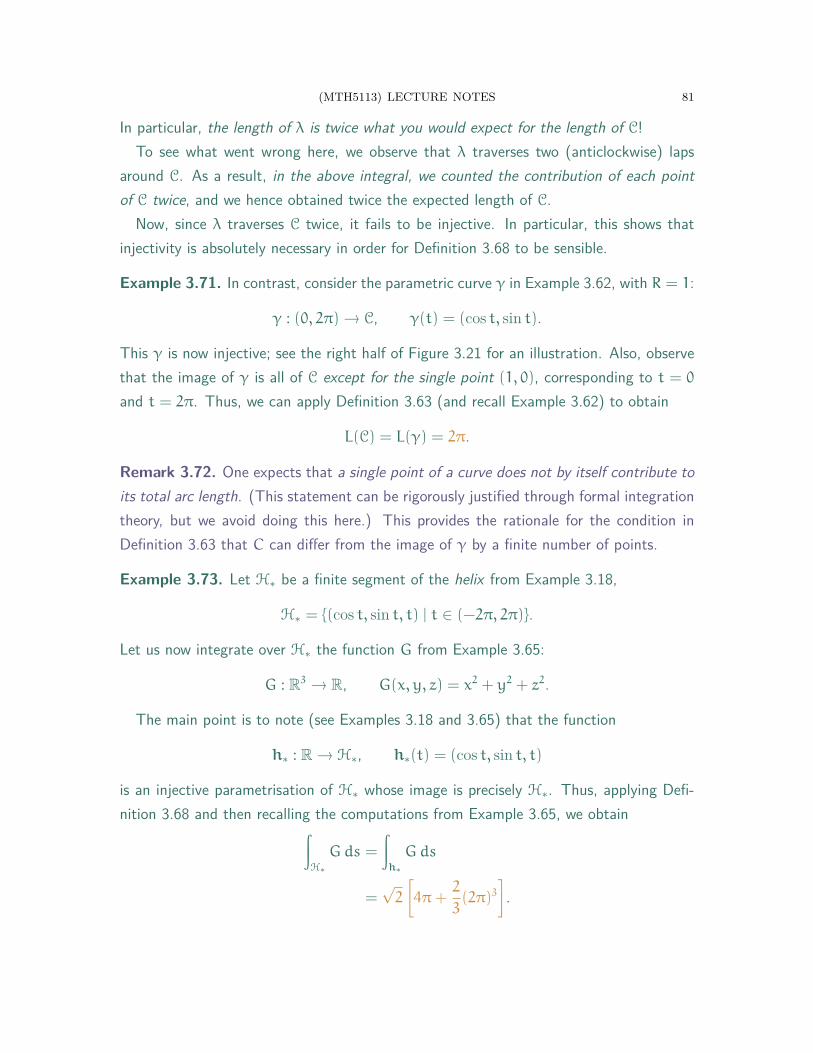
(MTH5113) LECTURE NOTES 81
In particular, the length of λ is twice what you would expect for the length of C!To see what went wrong here, we observe that λ traverses two (anticlockwise) laps
around C. As a result, in the above integral, we counted the contribution of each pointof C twice, and we hence obtained twice the expected length of C.
Now, since λ traverses C twice, it fails to be injective. In particular, this shows thatinjectivity is absolutely necessary in order for Definition 3.68 to be sensible.
Example 3.71. In contrast, consider the parametric curve γ in Example 3.62, with R = 1:
γ : (0, 2π) → C, γ(t) = (cos t, sin t).
This γ is now injective; see the right half of Figure 3.21 for an illustration. Also, observethat the image of γ is all of C except for the single point (1, 0), corresponding to t = 0
and t = 2π. Thus, we can apply Definition 3.63 (and recall Example 3.62) to obtain
L(C) = L(γ) = 2π.
Remark 3.72. One expects that a single point of a curve does not by itself contribute toits total arc length. (This statement can be rigorously justified through formal integrationtheory, but we avoid doing this here.) This provides the rationale for the condition inDefinition 3.63 that C can differ from the image of γ by a finite number of points.
Example 3.73. Let H∗ be a finite segment of the helix from Example 3.18,
H∗ = {(cos t, sin t, t) | t ∈ (−2π, 2π)}.
Let us now integrate over H∗ the function G from Example 3.65:
G : R3 → R, G(x, y, z) = x2 + y2 + z2.
The main point is to note (see Examples 3.18 and 3.65) that the function
h∗ : R → H∗, h∗(t) = (cos t, sin t, t)
is an injective parametrisation of H∗ whose image is precisely H∗. Thus, applying Defi-nition 3.68 and then recalling the computations from Example 3.65, we obtain∫
H∗
Gds =
∫h∗
Gds
=√2
[4π+
2
3(2π)3
].

82 (MTH5113) LECTURE NOTES
Example 3.74. Let C be the unit circle from Example 3.70, and let
F : R2 → R, F(x, y) = y.
To integrate F over C, we recall that γ, from Example 3.71, is an injective parametrisationof C, and that its image is C \ {(1, 0)}. Thus, by Definitions 3.63 and 3.68,∫
C
F ds =
∫ 2π
0
F(γ(t))|γ ′(t)|dt.
Now, from the definitions of F and γ, we have
|γ ′(t)| = 1, F(γ(t)) = sin t.
As a result of the above, we conclude that∫C
F ds =
∫ 2π
0
sin t dt
= 0.
3.10. Integration of Vector Fields. Next, we introduce a different type of curveintegration—an integral along an oriented curve of a vector field.
Of course, we should first ask why we would want to make such a definition. Onereason is that such integrals often come up in physics. An example is the notion ofwork in classical mechanics, which can be viewed as “force applied over a distance”.
Suppose there is a crate lying on the ground, and suppose you apply a force to thecrate by pushing it in a certain direction, such as in the left drawing of Figure 3.22.This force can be modelled by a vector field F in R3; at a point p ∈ R3, the arrow
F(p) = (F1(p), F2(p), F3(p))p,
represents you standing at p and applying force in the direction (F1(p), F2(p), F3(p)).Suppose that as you apply this force to the crate, it slides along a path given by a
curve C in R3. Since this crate has travelled some distance as you applied force to it,you might claim that you have done work (in the physics sense).
But wait! There is still a question of how productive your force was. If the cratemoved in the direction that you applied the force, as is the case in the middle drawingof Figure 3.22, then you can be happy with the fact that your force was effective.
On the other hand, suppose you push the crate rightwards, say, but it is movingdownwards in a perpendicular direction, as is depicted in the right drawing in Figure

(MTH5113) LECTURE NOTES 83
3.22. Even though you might be working (in a non-physics sense) hard, your force isnot so productive; in the physics sense, you have done no work on the box. Moreover,if you push the crate one way, and the crate is instead moving the other way, thenthe outcome is opposite to your intention, and negative work has been done!
Figure 3.22. The first drawing shows a person applying a force to a box.In the second illustration, the box moves in the direction of the force, sopositive work is being done by the force. In the third illustration, the boxmoves in a direction perpendicular to the force, so no work is being done.
Consequently, when measuring work, the only part of the force F that counts is thecomponent of F that points along the direction of the curve. If you remember yourbasic vector geometry, then you will recall that this component can be captured bytaking a dot product of F with a unit vector in the direction of the curve.
Putting all these ideas together, we end up at the following definition:
Definition 3.75. Let C ⊆ Rn be an oriented curve, and let F be a vector field on asubset of Rn containing C. Then, we define the curve integral of F over C by
(3.21)∫C
F · ds =
∫C
(F · t)ds,
where t denotes the unit tangents of C in the direction specified by the orientation of C,and where the integral on the right-hand side is defined as in (3.18).
First, note that since t, in Definition 3.75, is the unit tangent in the direction of C,then F · t indeed captures the component of F along C. Also, as F · t is scalar-valued,the right-hand integral in (3.21) can indeed be interpreted as in Definition 3.68.
Next, we ask the following: to what extent are curve integrals of vector fields geomet-ric, that is, independent of parametrisation? One observation, already noted above,is that the right-hand side of (3.21) is a curve integral of a scalar function, which wealready know is parametrisation-independent by Theorem 3.67.
However, what slightly complicates this discussion is the unit tangent t. If wereverse the orientation of C, then the corresponding unit tangent t is replaced by −t.

84 (MTH5113) LECTURE NOTES
Since everything else in the right-hand side of (3.21) is geometric and independent ofparametrisation, we arrive at the following:
Theorem 3.76. Let C and F be as in Definition 3.75, and let C∗ be the same curve asC, but given the opposite orientation. Then, we have that
(3.22)∫C∗
F · ds = −
∫C
F · ds.
In other words, Theorem 3.76 implies that curve integrals of vector fields are notquite geometric properties of curves, but they are properties of oriented curves.
To be more concrete, we return to our informal discussion of work that motivatedDefinition 3.75. If we apply a force to the crate, then whether the work done is positiveor negative depends on whether the crate moves in or opposite to the direction of theforce. Thus, the work done is sensitive to the direction that the crate travels.
Moving on to more practical matters, we now discuss how vector integrals can becomputed. The next theorem shows that they, like scalar integrals, can be computedvia parametrisations, except that we must be careful about orientation:
Theorem 3.77. Let C, F be as in Definition 3.75, and let γ : (a, b) → C be an injectiveparametrisation of C whose image differs from C by only a finite number of points.
• If γ generates the orientation of C, then
(3.23)∫C
F · ds = +
∫b
a
[F(γ(t)) · γ ′(t)γ(t)
]dt.
• If γ generates the orientation opposite to that of C, then
(3.24)∫C
F · ds = −
∫b
a
[F(γ(t)) · γ ′(t)γ(t)
]dt.
Proof. First, if γ generates the orientation of C, then Theorem 3.41 and Definition3.52 imply that the unit tangent t chosen by the orientation at the point γ(t) is givenby +|γ ′(t)|−1 · γ ′(t)γ(t). Thus, using Definitions 3.63, 3.68, and 3.75, we have∫
C
F · ds =
∫b
a
{F(γ(t)) ·
[+
γ ′(t)
|γ ′(t)|
]γ(t)
}|γ ′(t)|dt
=
∫b
a
[F(γ(t)) · γ ′(t)γ(t)
]dt.
The remaining case (3.24), in which γ generates the opposite orientation to C, isanalogous, except that t now corresponds to −|γ ′(t)|−1 · γ ′(t)γ(t). □
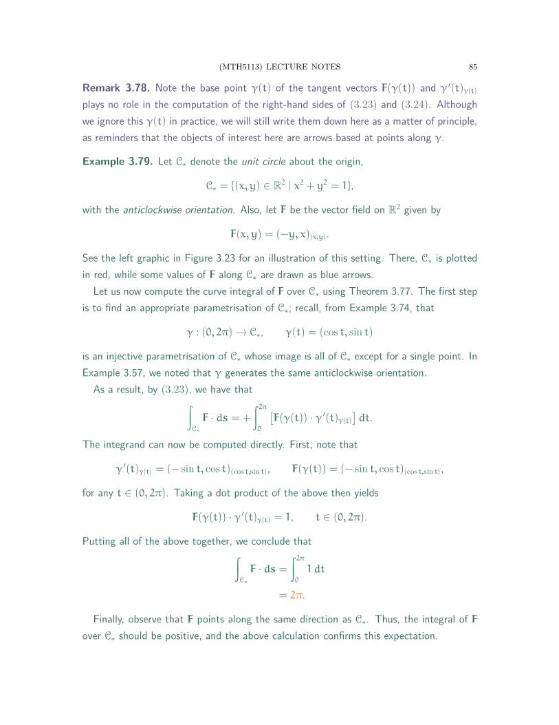
(MTH5113) LECTURE NOTES 85
Remark 3.78. Note the base point γ(t) of the tangent vectors F(γ(t)) and γ ′(t)γ(t)
plays no role in the computation of the right-hand sides of (3.23) and (3.24). Althoughwe ignore this γ(t) in practice, we will still write them down here as a matter of principle,as reminders that the objects of interest here are arrows based at points along γ.
Example 3.79. Let C∗ denote the unit circle about the origin,
C∗ = {(x, y) ∈ R2 | x2 + y2 = 1},
with the anticlockwise orientation. Also, let F be the vector field on R2 given by
F(x, y) = (−y, x)(x,y).
See the left graphic in Figure 3.23 for an illustration of this setting. There, C∗ is plottedin red, while some values of F along C∗ are drawn as blue arrows.
Let us now compute the curve integral of F over C∗ using Theorem 3.77. The first stepis to find an appropriate parametrisation of C∗; recall, from Example 3.74, that
γ : (0, 2π) → C∗, γ(t) = (cos t, sin t)
is an injective parametrisation of C∗ whose image is all of C∗ except for a single point. InExample 3.57, we noted that γ generates the same anticlockwise orientation.
As a result, by (3.23), we have that∫C∗
F · ds = +
∫ 2π
0
[F(γ(t)) · γ ′(t)γ(t)
]dt.
The integrand can now be computed directly. First, note that
γ ′(t)γ(t) = (− sin t, cos t)(cos t,sin t), F(γ(t)) = (− sin t, cos t)(cos t,sin t),
for any t ∈ (0, 2π). Taking a dot product of the above then yields
F(γ(t)) · γ ′(t)γ(t) = 1, t ∈ (0, 2π).
Putting all of the above together, we conclude that∫C∗
F · ds =
∫ 2π
0
1 dt
= 2π.
Finally, observe that F points along the same direction as C∗. Thus, the integral of Fover C∗ should be positive, and the above calculation confirms this expectation.

86 (MTH5113) LECTURE NOTES
−2 −1 1 2
−2
−1
1
2
x
y C∗
−1 1
−1
1
x
y
P∗
Figure 3.23. The left plot shows the setting of Example 3.79, with theoriented circle C∗ in red and values of F in blue. The right plot is the settingof Example 3.80, with the parabola P∗ in red and values of H in blue.
Example 3.80. Let P∗ denote the parabolic segment
P∗ = {(t, t2) | −1 < t < 1},
oriented in the direction of decreasing x-value. (Note P∗ is a curve by Theorem 3.28.)Let us integrate over P∗ the vector field H on R2 defined as
H(x, y) = (y, 0)(x,y).
First, observe that P∗ can be injectively parametrised in its entirety by
λ : (−1, 1) → R2, λ(t) = (t, t2).
The usual computations then yield, for each t ∈ (−1, 1),
F(λ(t)) · λ ′(t)λ(t) = (t2, 0) · (1, 2t)
= t2.
However, note that λ generates the orientation in the direction of increasing x-value,which is opposite to our given orientation for P∗. Thus, we apply (3.24) and obtain∫
P∗
F · ds = −
∫ 1
−1
t2 dt
= −2
3.
See the right graphic in Figure 3.23 for an illustration of P∗ (drawn in red), as well assome values of H along P∗ (drawn as blue arrows).

(MTH5113) LECTURE NOTES 87
Remark 3.81. Lastly, assume the setting of Definition 3.75, and expand F as
F(p) = (F1(p), . . . , Fn(p))p, p ∈ C.
In many calculus texts, the curve integral of F over C is often written as∫C
F · ds =
∫C
(F1 dx1 + F2 dx2 + · · ·+ Fn dxn).
(When n ≤ 3, one often writes dx, dy, dz in the place of dx1, dx2, dx3.) Formally speak-ing, the integrand on the right-hand side is known as a differential form. Unfortunately,the theory behind these objects lies beyond the scope of this module.

88 (MTH5113) LECTURE NOTES
4. The Geometry of Surfaces
In this portion of the module, we turn our attention toward the differential geometryof surfaces. You have probably heard the word “surface” used in many real-worldcontexts, such as “surface of a table” or “surface of the earth”. More abstractly, onecan view surfaces as “2-dimensional geometric objects”.
However, for a systematic study, one need a more precise description of surfaces.Thus, like for curves, we spend the first part of the chapter addressing the following:
Question 4.1. When we say “surface”, what exactly do we mathematically mean?
As we shall see, there will be some novel challenges in describing surfaces that wedid not previously encounter when studying curves.
4.1. Parametric Surfaces. Recall our discussions of curves began with the notionof parametric curves, which were used to map out the points of the underlying curve.Moreover, the expectation that parametric curves are “1-dimensional” is captured bytheir domains, which were open intervals in the (1-dimensional) real line.
We now employ a similar beginning to surface theory. The idea is once again toparametrise the points of a surface using vector-valued functions. Since we wish forsurfaces to be “2-dimensional” in nature, then the above suggests that we should nowconsider vector-valued functions whose domains are subsets of R2.
This leads us to our 2-dimensional analogue of parametric curves:
Definition 4.2. A parametric surface is a smooth vector-valued function σ : U → Rn,where n is a positive integer, and where U is an open and connected subset of R2.
In Definition 4.2, the condition that σ is smooth means that we can take as manypartial derivatives of σ as we wish, as all such derivatives are assumed to exist.
Remark 4.3. Although Definition 4.2 allows for parametric surfaces lying in any Rn,almost all of our examples will be in the special case n = 3.
Example 4.4. First, recall the parametric cylinder from Examples 2.23 and 2.55:
σ : R2 → R3, σ(u, v) = (cosu, sinu, v).
In particular, observe that the domain R2 of σ is both open and connected, thus σ isindeed a parametric surface. We also recall from the aforementioned examples that theimage of σ is a cylinder of unit radius about the z-axis; see the left plot of Figure 4.1.
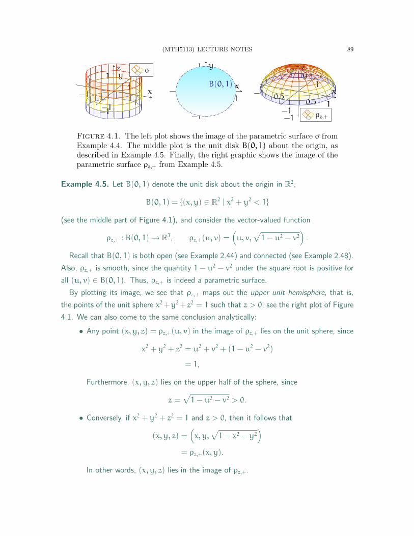
(MTH5113) LECTURE NOTES 89
−11
−1
1
−1
1
x
yz σ
−1 1
−1
1
B(0, 1) x
y
−1 −0.50.5 1
−1
1
−1
1
x
yz
ρz,+
Figure 4.1. The left plot shows the image of the parametric surface σ fromExample 4.4. The middle plot is the unit disk B(0, 1) about the origin, asdescribed in Example 4.5. Finally, the right graphic shows the image of theparametric surface ρz,+ from Example 4.5.
Example 4.5. Let B(0, 1) denote the unit disk about the origin in R2,
B(0, 1) = {(x, y) ∈ R2 | x2 + y2 < 1}
(see the middle part of Figure 4.1), and consider the vector-valued function
ρz,+ : B(0, 1) → R3, ρz,+(u, v) =(u, v,
√1− u2 − v2
).
Recall that B(0, 1) is both open (see Example 2.44) and connected (see Example 2.48).Also, ρz,+ is smooth, since the quantity 1− u2 − v2 under the square root is positive forall (u, v) ∈ B(0, 1). Thus, ρz,+ is indeed a parametric surface.
By plotting its image, we see that ρz,+ maps out the upper unit hemisphere, that is,the points of the unit sphere x2+y2+z2 = 1 such that z > 0; see the right plot of Figure4.1. We can also come to the same conclusion analytically:
• Any point (x, y, z) = ρz,+(u, v) in the image of ρz,+ lies on the unit sphere, since
x2 + y2 + z2 = u2 + v2 + (1− u2 − v2)
= 1,
Furthermore, (x, y, z) lies on the upper half of the sphere, since
z =√
1− u2 − v2 > 0.
• Conversely, if x2 + y2 + z2 = 1 and z > 0, then it follows that
(x, y, z) =(x, y,
√1− x2 − y2
)= ρz,+(x, y).
In other words, (x, y, z) lies in the image of ρz,+.
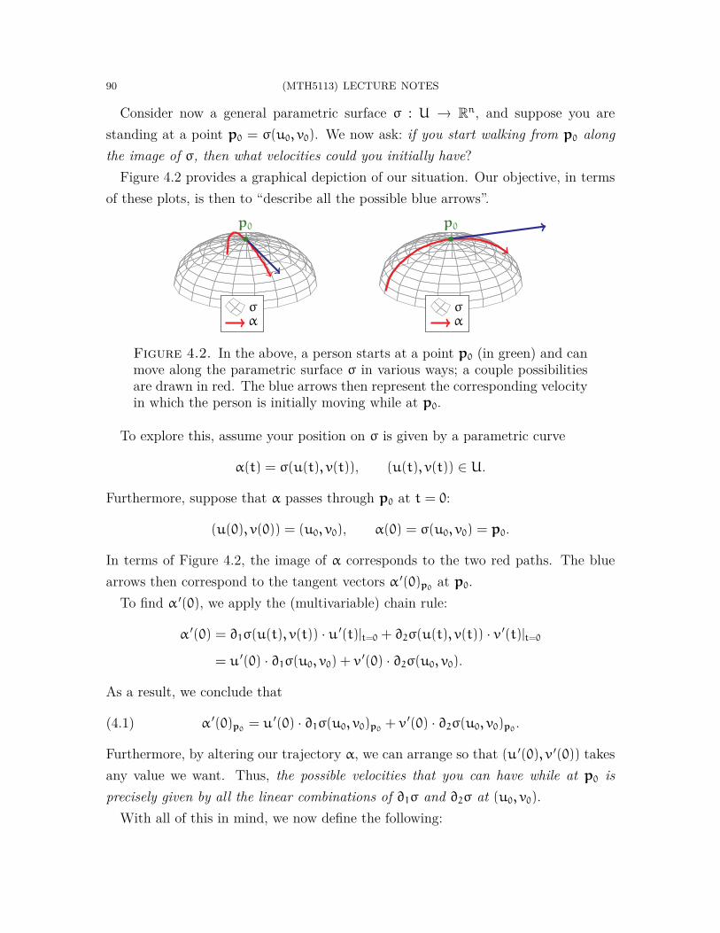
90 (MTH5113) LECTURE NOTES
Consider now a general parametric surface σ : U → Rn, and suppose you arestanding at a point p0 = σ(u0, v0). We now ask: if you start walking from p0 alongthe image of σ, then what velocities could you initially have?
Figure 4.2 provides a graphical depiction of our situation. Our objective, in termsof these plots, is then to “describe all the possible blue arrows”.
p0
σα
p0
σα
Figure 4.2. In the above, a person starts at a point p0 (in green) and canmove along the parametric surface σ in various ways; a couple possibilitiesare drawn in red. The blue arrows then represent the corresponding velocityin which the person is initially moving while at p0.
To explore this, assume your position on σ is given by a parametric curve
α(t) = σ(u(t), v(t)), (u(t), v(t)) ∈ U.
Furthermore, suppose that α passes through p0 at t = 0:
(u(0), v(0)) = (u0, v0), α(0) = σ(u0, v0) = p0.
In terms of Figure 4.2, the image of α corresponds to the two red paths. The bluearrows then correspond to the tangent vectors α ′(0)p0
at p0.To find α ′(0), we apply the (multivariable) chain rule:
α ′(0) = ∂1σ(u(t), v(t)) · u ′(t)|t=0 + ∂2σ(u(t), v(t)) · v ′(t)|t=0
= u ′(0) · ∂1σ(u0, v0) + v ′(0) · ∂2σ(u0, v0).
As a result, we conclude that
(4.1) α ′(0)p0= u ′(0) · ∂1σ(u0, v0)p0
+ v ′(0) · ∂2σ(u0, v0)p0.
Furthermore, by altering our trajectory α, we can arrange so that (u ′(0), v ′(0)) takesany value we want. Thus, the possible velocities that you can have while at p0 isprecisely given by all the linear combinations of ∂1σ and ∂2σ at (u0, v0).
With all of this in mind, we now define the following:

(MTH5113) LECTURE NOTES 91
Definition 4.6. Let σ : U → Rn be a parametric surface, and let (u0, v0) ∈ U. Then,the tangent plane to σ at (u0, v0) is defined to be the following set:
(4.2) Tσ(u0, v0) ={a · ∂1σ(u0, v0)σ(u0,v0) + b · ∂2σ(u0, v0)σ(u0,v0)
∣∣a, b ∈ R}
.
Remark 4.7. Observe that Tσ(u0, v0), in Definition 4.6, is a vector space, since it is thelinear span of the tangent vectors ∂1σ(u0, v0)σ(u0,v0) and ∂2σ(u0, v0)σ(u0,v0).
−1
1−1
1
−1
1
ρz,+(0, 0)
x
y
z
ρz,+
−1
1−1
1
−1
1
x
y
z
ρz,+
Tρz,+(0, 0)
Figure 4.3. The left plot shows the image of ρz,+ from Example 4.8. In theright graphic, the arrows ∂1ρz,+(0, 0)ρz,+(0,0) (in blue) and ∂2ρz,+(0, 0)ρz,+(0,0)
(in purple) are drawn on the image of ρz,+. Moreover, the tangent planeTρz,+(0, 0) is represented as a plane lying on top of ρz,+.
Example 4.8. Consider first the parametric upper hemisphere from Example 4.5:
ρz,+ : B(0, 1) → R3, ρz,+(u, v) =(u, v,
√1− u2 − v2
).
See the left half of Figure 4.3 for a plot of ρz,+. Let us find the tangent plane Tρz,+(0, 0),i.e. the velocities along ρz,+ with which one can go from ρz,+(0, 0) = (0, 0, 1).
By Definition 4.6, the first step is to compute the partial derivatives of ρz,+. To find∂1ρz,+, we differentiate each component of ρz,+ with respect to the first variable u:
∂1ρz,+(u, v) =
(1, 0,
1
2· ∂u(1− u2 − v2)√
1− u2 − v2
)=
(1, 0,−
u√1− u2 − v2
).
A similar differentiation with respect to v yields that
∂2ρz,+(u, v) =
(0, 1,−
v√1− u2 − v2
).
In particular, at (u, v) = (0, 0), we have
∂1ρz,+(0, 0) = (1, 0, 0), ∂2ρz,+(0, 0) = (0, 1, 0).

92 (MTH5113) LECTURE NOTES
Therefore, by (4.2), our desired tangent plane of ρz,+ is
Tρz,+(0, 0) ={a · ∂1ρz,+(0, 0)ρz,+(0,0) + b · ∂2ρz,+(0, 0)ρz,+(0,0)
∣∣a, b ∈ R}
={a · (1, 0, 0)(0,0,1) + b · (0, 1, 0)(0,0,1)
∣∣a, b ∈ R}
.
The graphic on the right-hand side of Figure 4.3 demonstrates the above setting. Thearrows ∂1ρz,+(0, 0)ρz,+(0,0) and ∂2ρz,+(0, 0)ρz,+(0,0) are drawn in blue and purple, respec-tively. All the tangent vectors within Tρz,+(0, 0) (i.e. the linear combinations of the blueand purple arrows) then generate a 2-dimensional plane, which is drawn on top of ρz,+.
−2
2−2
2
−2
2
τ(0, 0)
x
yz
τ
−2
2−2
2
−2
2
x
yz
τ
Tτ(0, 0)
Figure 4.4. The left graphic shows the torus τ from Example 4.9. Theright drawing also contains both ∂1τ(0, 0)τ(0,0) (in blue) and ∂2τ(0, 0)τ(0,0)(in purple), as well as the tangent plane Tτ(0, 0).
Example 4.9. Next, consider the vector-valued function
τ : R2 → R3, τ(u, v) = ((2+ cosu) cos v, (2+ cosu) sin v, sinu),
which satisfies all the conditions of Definition 4.2 and hence is a parametric surface. The“doughnut-shaped” image of τ, called a torus, is drawn in the left part of Figure 4.4.
Let us now compute Tτ(0, 0). First, some direct computations yield that
∂1τ(u, v) = (− sinu cos v,− sinu sin v, cosu),
∂2τ(u, v) = (−(2+ cosu) sin v, (2+ cosu) cos v, 0).
In particular, at (u, v) = (0, 0),
∂1τ(0, 0)τ(0,0) = (0, 0, 1)(3,0,0), ∂2τ(0, 0)τ(0,0) = (0, 3, 0)(3,0,0).
Thus, using Definition 4.2, we conclude that
Tτ(0, 0) = {a · (0, 0, 1)(3,0,0) + b · (0, 3, 0)(3,0,0) | a, b ∈ R}.
See the right plot of Figure 4.4 for an illustration of Tτ(0, 0).
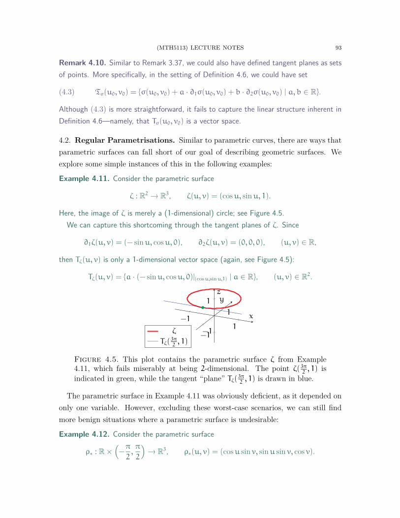
(MTH5113) LECTURE NOTES 93
Remark 4.10. Similar to Remark 3.37, we could also have defined tangent planes as setsof points. More specifically, in the setting of Definition 4.6, we could have set
(4.3) Tσ(u0, v0) = {σ(u0, v0) + a · ∂1σ(u0, v0) + b · ∂2σ(u0, v0) | a, b ∈ R}.
Although (4.3) is more straightforward, it fails to capture the linear structure inherent inDefinition 4.6—namely, that Tσ(u0, v0) is a vector space.
4.2. Regular Parametrisations. Similar to parametric curves, there are ways thatparametric surfaces can fall short of our goal of describing geometric surfaces. Weexplore some simple instances of this in the following examples:
Example 4.11. Consider the parametric surface
ζ : R2 → R3, ζ(u, v) = (cosu, sinu, 1).
Here, the image of ζ is merely a (1-dimensional) circle; see Figure 4.5.We can capture this shortcoming through the tangent planes of ζ. Since
∂1ζ(u, v) = (− sinu, cosu, 0), ∂2ζ(u, v) = (0, 0, 0), (u, v) ∈ R,
then Tζ(u, v) is only a 1-dimensional vector space (again, see Figure 4.5):
Tζ(u, v) = {a · (− sinu, cosu, 0)|(cosu,sinu,1) | a ∈ R}, (u, v) ∈ R2.
−11
−1
1
−1
1
x
yz
ζ
Tζ(3π2, 1)
Figure 4.5. This plot contains the parametric surface ζ from Example4.11, which fails miserably at being 2-dimensional. The point ζ( 3π
2, 1) is
indicated in green, while the tangent “plane” Tζ(3π2, 1) is drawn in blue.
The parametric surface in Example 4.11 was obviously deficient, as it depended ononly one variable. However, excluding these worst-case scenarios, we can still findmore benign situations where a parametric surface is undesirable:
Example 4.12. Consider the parametric surface
ρ∗ : R×(−π
2,π
2
)→ R3, ρ∗(u, v) = (cosu sin v, sinu sin v, cos v).
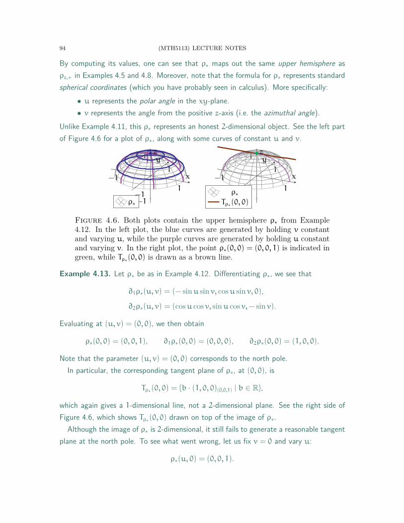
94 (MTH5113) LECTURE NOTES
By computing its values, one can see that ρ∗ maps out the same upper hemisphere asρz,+ in Examples 4.5 and 4.8. Moreover, note that the formula for ρ∗ represents standardspherical coordinates (which you have probably seen in calculus). More specifically:
• u represents the polar angle in the xy-plane.• v represents the angle from the positive z-axis (i.e. the azimuthal angle).
Unlike Example 4.11, this ρ∗ represents an honest 2-dimensional object. See the left partof Figure 4.6 for a plot of ρ∗, along with some curves of constant u and v.
−1
1−1
1
−1
1
x
yz
ρ∗
−1
1−1
1
−1
1
x
yz
ρ∗Tρ∗(0, 0)
Figure 4.6. Both plots contain the upper hemisphere ρ∗ from Example4.12. In the left plot, the blue curves are generated by holding v constantand varying u, while the purple curves are generated by holding u constantand varying v. In the right plot, the point ρ∗(0, 0) = (0, 0, 1) is indicated ingreen, while Tρ∗(0, 0) is drawn as a brown line.
Example 4.13. Let ρ∗ be as in Example 4.12. Differentiating ρ∗, we see that
∂1ρ∗(u, v) = (− sinu sin v, cosu sin v, 0),
∂2ρ∗(u, v) = (cosu cos v, sinu cos v,− sin v).
Evaluating at (u, v) = (0, 0), we then obtain
ρ∗(0, 0) = (0, 0, 1), ∂1ρ∗(0, 0) = (0, 0, 0), ∂2ρ∗(0, 0) = (1, 0, 0).
Note that the parameter (u, v) = (0, 0) corresponds to the north pole.In particular, the corresponding tangent plane of ρ∗, at (0, 0), is
Tρ∗(0, 0) = {b · (1, 0, 0)(0,0,1) | b ∈ R},
which again gives a 1-dimensional line, not a 2-dimensional plane. See the right side ofFigure 4.6, which shows Tρ∗(0, 0) drawn on top of the image of ρ∗.
Although the image of ρ∗ is 2-dimensional, it still fails to generate a reasonable tangentplane at the north pole. To see what went wrong, let us fix v = 0 and vary u:
ρ∗(u, 0) = (0, 0, 1).

(MTH5113) LECTURE NOTES 95
In particular, when v = 0, varying u does not change the value of ρ∗. This results in theloss of the “u-dimension” from the tangent plane Tρ∗(0, 0).
One consequence of this is that ρ∗ is an undesirable way to parametrise the upperhemisphere. Even though the upper hemisphere itself is genuinely 2-dimensional, theparametric surface ρ∗ still fails to be 2-dimensional at the north pole.
What is needed, then, for a parametric surface to be “2-dimensional”? Recall thatthe tangent planes of a parametric surface σ capture all the directions that one canmove along σ. Thus, for σ to be truly 2-dimensional, there should be two dimensionsof directions that one can move along σ, i.e. the Tσ(u, v)’s should be 2-dimensional.
Definition 4.14. A parametric surface σ : U → Rn is regular iff for any (u, v) ∈ U, thevectors ∂1σ(u, v) and ∂2σ(u, v) are linearly independent.
To better understand Definition 4.14, we recall a bit of linear algebra. Notice thatDefinition 4.14 implies σ is regular if and only if ∂1σ(u, v) and ∂2σ(u, v) always spana 2-dimensional vector space. By (4.2), this is true if and only if Tσ(u, v) is also a2-dimensional vector space. Thus, we can now conclude the following:
Theorem 4.15. A parametric surface σ : U → Rn is regular if and only if Tσ(u, v) isa 2-dimensional vector space for any (u, v) ∈ U. Moreover, when σ is regular, then∂1σ(u, v)σ(u,v) and ∂2σ(u, v)σ(u,v) form a basis for Tσ(u, v), for any (u, v) ∈ U.
Example 4.16. Recall our previous description of the upper hemisphere,
ρz,+ : B(0, 1) → R3, ρz,+(u, v) =(u, v,
√1− u2 − v2
).
from Example 4.8. There, we have already computed the partial derivatives of ρz,+:
∂1ρz,+(u, v) =
(1, 0,−
u√1− u2 − v2
),
∂2ρz,+(u, v) =
(0, 1,−
v√1− u2 − v2
).
For any (u, v) ∈ B(0, 1), the vector ∂1ρz,+(u, v) always has a nonzero x-componentand a zero y-component, while ∂2ρz,+(u, v) always has a nonzero y-component and a zerox-component. Therefore, ∂1ρz,+(u, v) and ∂2ρz,+(u, v) always point in different directionsand hence are linearly independent. By Definition 4.14, we conclude ρz,+ is regular.
In Example 4.16, it was clear by inspection that ∂1ρz,+ and ∂2ρz,+ are everywherelinearly independent. In general, however, this may not be so simple. Thus, we ask
96 (MTH5113) LECTURE NOTES
whether there is a computational method to check whether a parametric surface isregular. A convenient method does exist for surfaces lying in 3-dimensional space:
Theorem 4.17. A parametric surface σ : U → R3 is regular if and only if
(4.4) |∂1σ(u, v)× ∂2σ(u, v)| 6= 0
for every parameter (u, v) ∈ U.
Proof. Recall from Theorem 2.18 that
|∂1σ(u, v)× ∂2σ(u, v)| = |∂1σ(u, v)||∂2σ(u, v)| · sin θ(u, v),
where θ(u, v) is the angle between ∂1σ(u, v)σ(u,v) and ∂2σ(u, v)σ(u,v). Thus, (4.4)holds if and only if both ∂uσ(u, v) and ∂vσ(u, v) are nonzero and sin θ(u, v) 6= 0.Furthermore, sin θ(u, v) is nonzero if and only if ∂1σ(u, v) and ∂2σ(u, v) point indifferent directions (and hence are linearly independent). Combining all the above,we conclude that (4.4) is indeed equivalent to σ being regular. □
Example 4.18. Consider the torus from Example 4.9 (see also Figure 4.4),
τ : R2 → R3, τ(u, v) = ((2+ cosu) cos v, (2+ cosu) sin v, sinu).
Recall also from Example 4.9 that
∂1τ(u, v) = (− sinu cos v,− sinu sin v, cosu),
∂2τ(u, v) = (−(2+ cosu) sin v, (2+ cosu) cos v, 0).
Taking a cross product of the above yields
∂1τ(u, v)× ∂2τ(u, v) = −(2+ cosu)(cosu cos v, cosu sin v, sinu),
for which the norm is
|∂1τ(u, v)× ∂2τ(u, v)| = (2+ cosu)(cos2 u cos2 v+ cos2 u sin2 v+ sin2 u)
= (2+ cosu)(cos2 u+ sin2 u)
= 2+ cosu.
Since the above is everywhere nonzero, Theorem 4.17 implies that τ is regular.
Remark 4.19. Similarly, note that a parametric curve γ is regular if and only if all of itstangent lines Tγ(t) are 1-dimensional vector spaces, i.e. they are actual lines.
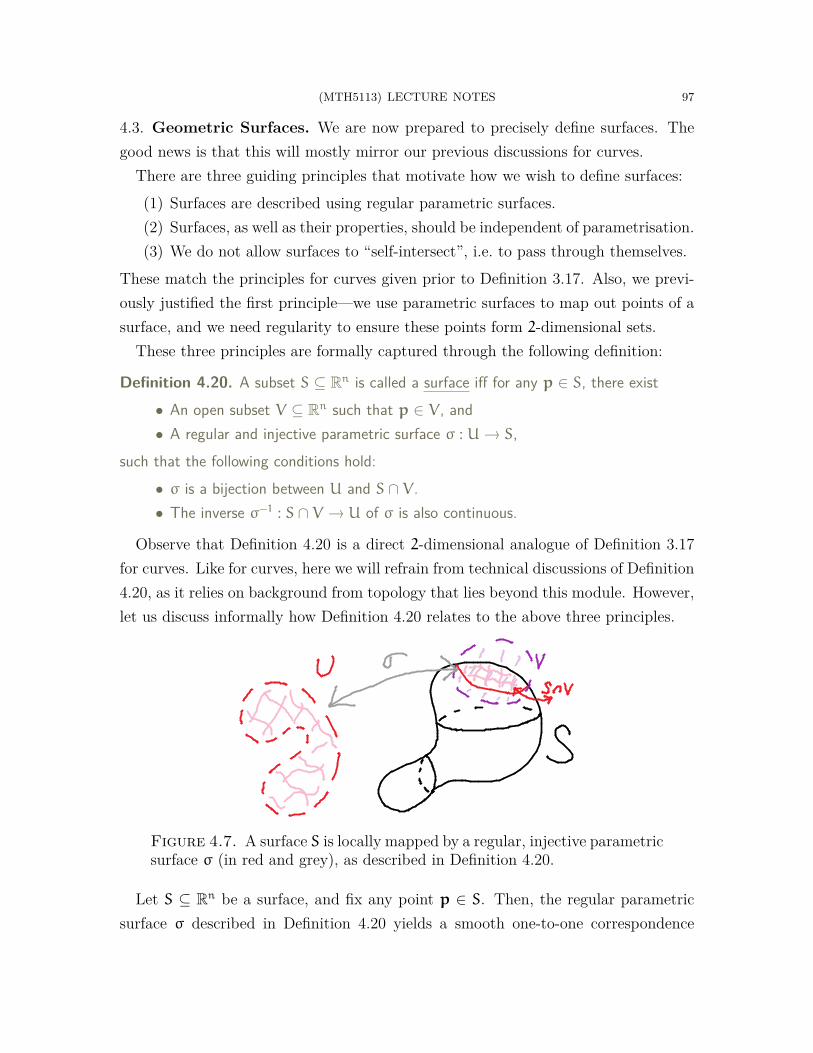
(MTH5113) LECTURE NOTES 97
4.3. Geometric Surfaces. We are now prepared to precisely define surfaces. Thegood news is that this will mostly mirror our previous discussions for curves.
There are three guiding principles that motivate how we wish to define surfaces:(1) Surfaces are described using regular parametric surfaces.(2) Surfaces, as well as their properties, should be independent of parametrisation.(3) We do not allow surfaces to “self-intersect”, i.e. to pass through themselves.
These match the principles for curves given prior to Definition 3.17. Also, we previ-ously justified the first principle—we use parametric surfaces to map out points of asurface, and we need regularity to ensure these points form 2-dimensional sets.
These three principles are formally captured through the following definition:
Definition 4.20. A subset S ⊆ Rn is called a surface iff for any p ∈ S, there exist• An open subset V ⊆ Rn such that p ∈ V , and• A regular and injective parametric surface σ : U → S,
such that the following conditions hold:• σ is a bijection between U and S ∩ V .• The inverse σ−1 : S ∩ V → U of σ is also continuous.
Observe that Definition 4.20 is a direct 2-dimensional analogue of Definition 3.17for curves. Like for curves, here we will refrain from technical discussions of Definition4.20, as it relies on background from topology that lies beyond this module. However,let us discuss informally how Definition 4.20 relates to the above three principles.
Figure 4.7. A surface S is locally mapped by a regular, injective parametricsurface σ (in red and grey), as described in Definition 4.20.
Let S ⊆ Rn be a surface, and fix any point p ∈ S. Then, the regular parametricsurface σ described in Definition 4.20 yields a smooth one-to-one correspondence
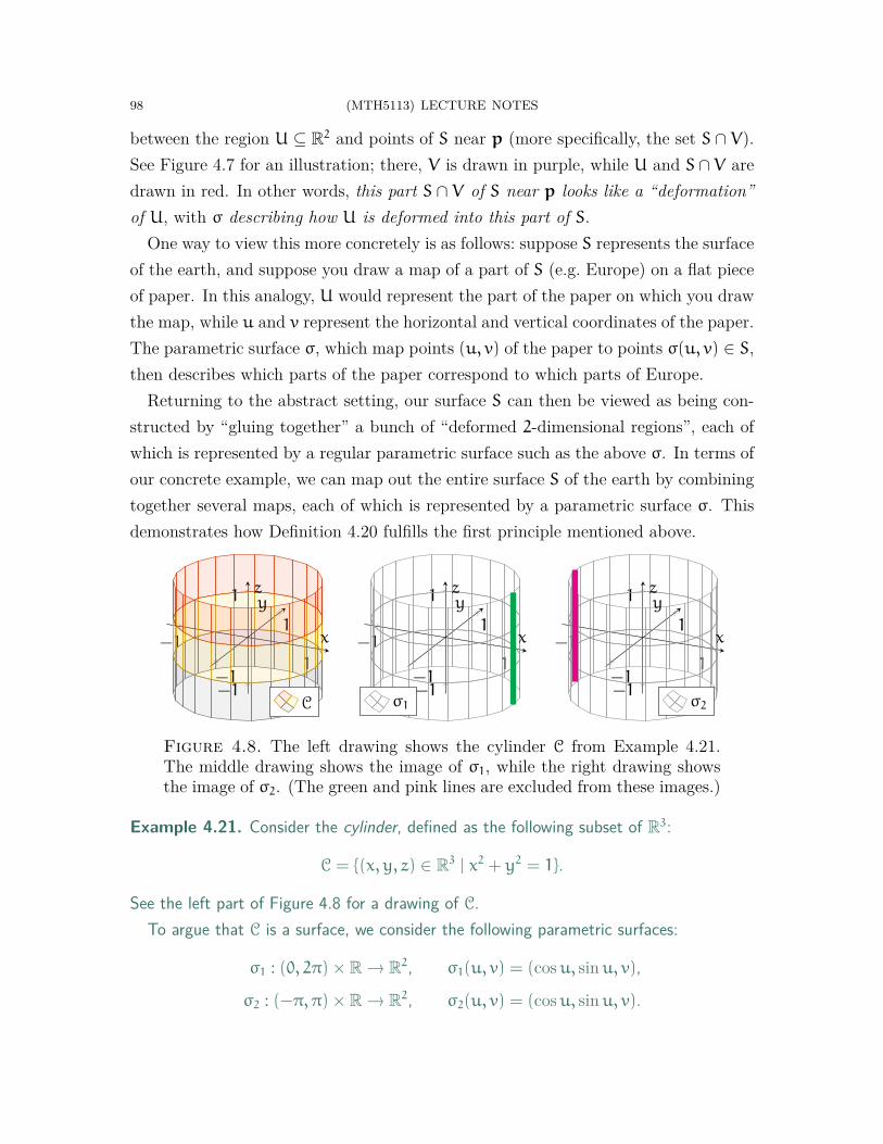
98 (MTH5113) LECTURE NOTES
between the region U ⊆ R2 and points of S near p (more specifically, the set S ∩ V).See Figure 4.7 for an illustration; there, V is drawn in purple, while U and S∩ V aredrawn in red. In other words, this part S ∩ V of S near p looks like a “deformation”of U, with σ describing how U is deformed into this part of S.
One way to view this more concretely is as follows: suppose S represents the surfaceof the earth, and suppose you draw a map of a part of S (e.g. Europe) on a flat pieceof paper. In this analogy, U would represent the part of the paper on which you drawthe map, while u and v represent the horizontal and vertical coordinates of the paper.The parametric surface σ, which map points (u, v) of the paper to points σ(u, v) ∈ S,then describes which parts of the paper correspond to which parts of Europe.
Returning to the abstract setting, our surface S can then be viewed as being con-structed by “gluing together” a bunch of “deformed 2-dimensional regions”, each ofwhich is represented by a regular parametric surface such as the above σ. In terms ofour concrete example, we can map out the entire surface S of the earth by combiningtogether several maps, each of which is represented by a parametric surface σ. Thisdemonstrates how Definition 4.20 fulfills the first principle mentioned above.
−1
1−1
1
−1
1
x
yz
C
−1
1−1
1
−1
1
x
yz
σ1
−1
1−1
1
−1
1
x
yz
σ2
Figure 4.8. The left drawing shows the cylinder C from Example 4.21.The middle drawing shows the image of σ1, while the right drawing showsthe image of σ2. (The green and pink lines are excluded from these images.)
Example 4.21. Consider the cylinder, defined as the following subset of R3:
C = {(x, y, z) ∈ R3 | x2 + y2 = 1}.
See the left part of Figure 4.8 for a drawing of C.To argue that C is a surface, we consider the following parametric surfaces:
σ1 : (0, 2π)× R → R2, σ1(u, v) = (cosu, sinu, v),
σ2 : (−π, π)× R → R2, σ2(u, v) = (cosu, sinu, v).
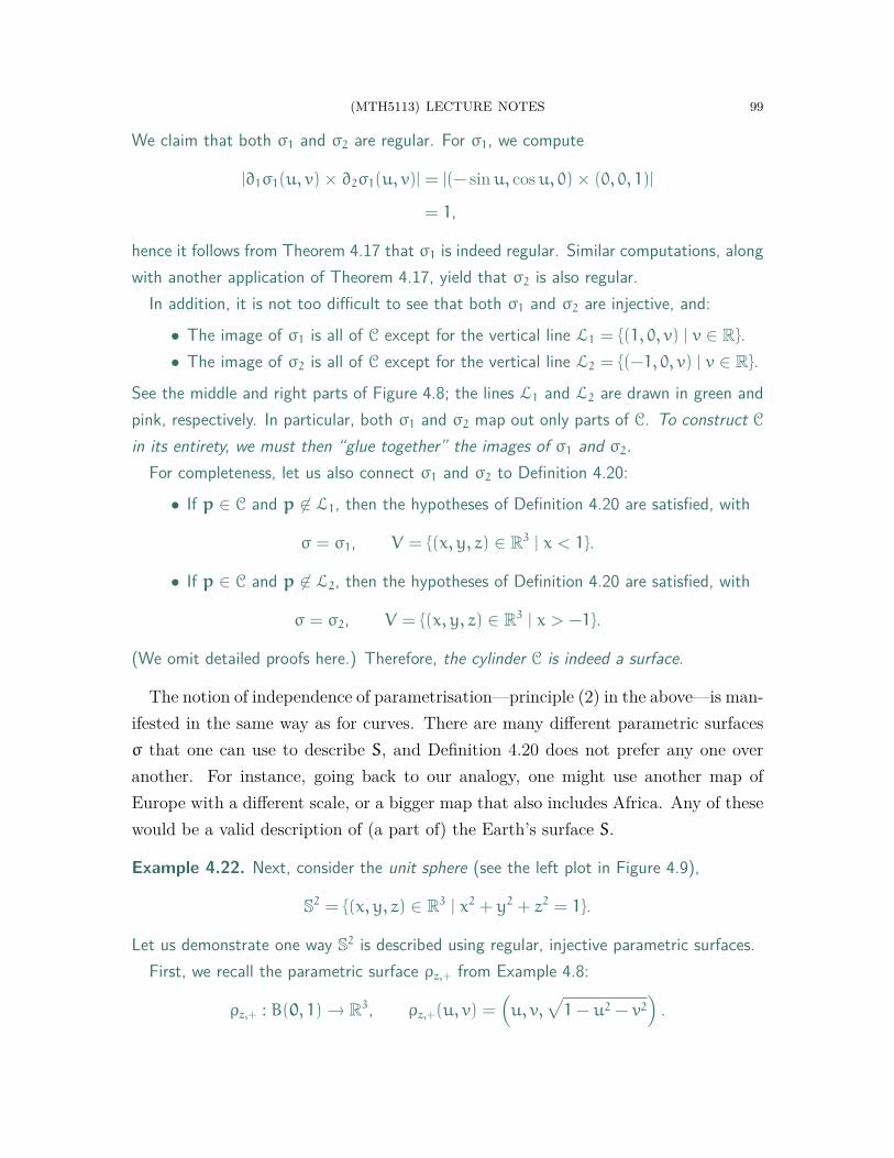
(MTH5113) LECTURE NOTES 99
We claim that both σ1 and σ2 are regular. For σ1, we compute
|∂1σ1(u, v)× ∂2σ1(u, v)| = |(− sinu, cosu, 0)× (0, 0, 1)|
= 1,
hence it follows from Theorem 4.17 that σ1 is indeed regular. Similar computations, alongwith another application of Theorem 4.17, yield that σ2 is also regular.
In addition, it is not too difficult to see that both σ1 and σ2 are injective, and:• The image of σ1 is all of C except for the vertical line L1 = {(1, 0, v) | v ∈ R}.• The image of σ2 is all of C except for the vertical line L2 = {(−1, 0, v) | v ∈ R}.
See the middle and right parts of Figure 4.8; the lines L1 and L2 are drawn in green andpink, respectively. In particular, both σ1 and σ2 map out only parts of C. To construct Cin its entirety, we must then “glue together” the images of σ1 and σ2.
For completeness, let us also connect σ1 and σ2 to Definition 4.20:• If p ∈ C and p 6∈ L1, then the hypotheses of Definition 4.20 are satisfied, with
σ = σ1, V = {(x, y, z) ∈ R3 | x < 1}.
• If p ∈ C and p 6∈ L2, then the hypotheses of Definition 4.20 are satisfied, with
σ = σ2, V = {(x, y, z) ∈ R3 | x > −1}.
(We omit detailed proofs here.) Therefore, the cylinder C is indeed a surface.
The notion of independence of parametrisation—principle (2) in the above—is man-ifested in the same way as for curves. There are many different parametric surfacesσ that one can use to describe S, and Definition 4.20 does not prefer any one overanother. For instance, going back to our analogy, one might use another map ofEurope with a different scale, or a bigger map that also includes Africa. Any of thesewould be a valid description of (a part of) the Earth’s surface S.
Example 4.22. Next, consider the unit sphere (see the left plot in Figure 4.9),
S2 = {(x, y, z) ∈ R3 | x2 + y2 + z2 = 1}.
Let us demonstrate one way S2 is described using regular, injective parametric surfaces.First, we recall the parametric surface ρz,+ from Example 4.8:
ρz,+ : B(0, 1) → R3, ρz,+(u, v) =(u, v,
√1− u2 − v2
).

100 (MTH5113) LECTURE NOTES
Observe that ρz,+ is injective, and the computations in Example 4.16 show that ρz,+ isregular. Moreover, Example 4.8 shows that the image of ρz,+ is the top half of the sphere:
{(x, y, z) ∈ S2 | z > 0}.
Next, to map the bottom half of the sphere, we simply negate the z-coordinate in ρz,+:
ρz,− : B(0, 1) → R3, ρz,−(u, v) =(u, v,−
√1− u2 − v2
).
Then, ρz,+ and ρz,− together cover all of S2, except for the equatorial circle z = 0.One (rather inefficient) way to cover this remaining equatorial circle is to define para-
metric surfaces that are like ρz,+ and ρz,−, except we switch around the roles of the threecoordinates. More specifically, we define the following four parametric surfaces:
ρy,± : B(0, 1) → R3, ρy,±(u, v) =(u, ±
√1− u2 − v2, v
),
ρx,± : B(0, 1) → R3, ρx,±(u, v) =(±√1− u2 − v2, u, v
).
Notice that all six of the above parametric surfaces are regular and injective.The right side of Figure 4.9 shows the images of all six parametric surfaces ρz,±, ρy,±,
ρx,±. Note that these parametric surfaces together describe the full sphere—that is, S2
can be constructed by “gluing together” the images of these six parametric surfaces.We also note that ρz,±, ρy,±, ρx,± can be used to formally show that S2 satisfies the
conditions of Definition 4.20 and hence is a surface. However, we omit the details here.
−1
1−1
1
−1
1
x
y
z
S2
−11
−1
1
−1
1
x
yz
σz,+
−11
−1
1
−1
1
x
yz
σy,+
−11
−1
1
−1
1
x
yzσx,+
−11
−1
1
−1
1
x
yzσz,−
−11
−1
1
−1
1
x
yzσy,−
−11
−1
1
−1
1
x
yz
σx,−
Figure 4.9. The left graphic is the sphere S2 from Example 4.22; the re-maining plots show the images of the parametric surfaces ρz,±, ρy,±, ρx,±.
Finally, we give an informal discussion of the third principle—namely, that a surfaceshould not be “self-intersecting”. For this, we consider the object S in the left drawingof Figure 4.10, and we let p be the self-intersecting green point on S. Then, given any

(MTH5113) LECTURE NOTES 101
open subset V as in Definition 4.20, the intersection S∩V must contain an “X-figure”around p made by two intersecting strips; see the right part of Figure 4.10.
−1
1−1
1
−1
1
x
yz
S
−1
1−1
1
−1
1
x
yz
S ∩ V
Figure 4.10. The object S in the above plots fails to be a surface. This isbecause at the green point p, any open subset V that contains p must alsocontain an “X-figure” with two strips crossing each other. One particularexample of this is illustrated in the drawing on the right.
The key point is that this X-figure has a different (topological) structure than anopen set U ⊆ R2. The conditions on σ in Definition 4.20 prevent it from being able tomap U onto this X-figure. To see this informally, you can convince yourself that it isnot possible to bend a piece of paper (representing U) into this X-figure without eithertearing it (violating continuity) or folding over itself (violating injectivity). Thus, weconclude that this S cannot satisfy Definition 4.20 and hence is not a surface.
Remark 4.23. The surfaces of Definition 4.20 are sometimes called embedded surfaces.One can, alternatively, study a more general class of 2-dimensional objects—immersedsurfaces—that are allowed to pass through themselves.
4.4. Descriptions of Surfaces. We now discuss some more practical methods forconstructing and describing surfaces. First, like for curves, it is often more convenientto describe surfaces using parametric surfaces that are not injective.
Definition 4.24. Let S ⊆ Rn be a surface. We refer to any regular (not necessarilyinjective) parametric surface σ : U → S as a parametrisation of S.Example 4.25. Consider again the cylinder from Example 4.21:
C = {(x, y, z) ∈ R3 | x2 + y2 = 1}.
In Example 4.21, we needed two injective regular parametric surfaces (σ1 and σ2) todescribe all of C. In fact, this is the best we can do, as one can show it is not possible tocover all of C using only a single injective and regular parametric surface.
102 (MTH5113) LECTURE NOTES
However, we can do better if we remove the requirement of injectivity. Indeed, let usconsider instead the parametric surface σ from Example 4.4:
σ : R2 → R3, σ(u, v) = (cosu, sinu, v).
Observe (see also Example 2.23) that the image of σ is precisely all of C. Furthermore,by the same computations as in Example 4.21, we obtain that σ is regular.
Thus, σ is a parametrisation of C whose image is all of C. On the other hand, σ failsto be injective; for example, σ(2πk, 0) = (1, 0, 0) for any k ∈ Z.
−1 −0.50.5 1
−1
1
−1
1
x
y
z
ρs,z
−1 −0.50.5 1
−1
1
−1
1
x
y
z
ρs,y
Figure 4.11. The two plots show the images of the parametrisations ρs,z
(left) and ρs,y (right) of S2 from Example 4.26. In each drawing, the pair ofpink-coloured points are excluded from the image.
Example 4.26. To contrast with the previous example, let us return to the sphere,
S2 = {(x, y, z) ∈ R3 | x2 + y2 + z2 = 1}.
Example 4.25 demonstrated that the cylinder C could be described using only a singleparametrisation. On the other hand, it is impossible to cover all of S2 using only oneparametrisation of S2, injective or not. (Sadly, we cannot give a proof of this here.)
Let us instead describe S2 using two parametrisations. There are many ways to do this,but here make use of spherical coordinates (see also Example 4.12):
ρs,z : R× (0, π) → S2, ρs,z(u, v) = (cosu sin v, sinu sin v, cos v).
To see that ρs,z is regular, we compute, for each (u, v) ∈ R× (0, π):
∂1ρs,z(u, v) = (− sinu sin v, cosu sin v, 0),
∂2ρs,z(u, v) = (cosu cos v, sinu cos v,− sin v).
Taking a cross product then yields
|∂1ρs,z(u, v)× ∂2ρs,z(u, v)| = |(− cosu sin2 v,− sinu sin2 v,− sin v cos v)|
(MTH5113) LECTURE NOTES 103
= | sin v| |(cosu sin v, sinu sin v, cos v)|
= sin v.
Since v ∈ (0, π), then sin v 6= 0, and Theorem 4.17 yields that ρs,z is regular.See the left part of Figure 4.11 for a plot of ρs,z. In particular, the image of ρs,z is
all of S2 except for the north pole (0, 0, 1) (corresponding to v = 0) and the south pole(0, 0,−1) (corresponding to v = π). We cannot include those two points into ρs,z, sincesin 0 = sinπ = 0, and hence the above computation implies that ρs,z cannot be regularif we also allow v = 0 and v = π into its domain.
To cover all of S2, we need a second parametrisation. An easy way to do this is to justpermute the components of ρs,z, so that two different points are excluded:
ρs,y : R× (0, π) → S2, ρs,y(u, v) = (sinu sin v, cos v, cosu sin v),
By similar reasoning, ρs,y is a parametrisation of S2, and its image is all of S2 except forthe points (0,±1, 0). Thus, the parametrisations ρs,z and ρs,y together cover all of S2.
Next, we state an analogue of Theorem 3.24 for surfaces—that level sets of suffi-ciently nice real-valued functions of three variables are surfaces:
Theorem 4.27. Suppose V ⊆ R3 is open and connected, and let f : V → R be a smoothfunction. Moreover, let c ∈ R, and let S denote the level set
S = {(x, y, z) ∈ V | f(x, y, z) = c}.
If ∇f(p) is nonzero for every p ∈ S, then S is a surface.
Due to lack of background, we omit the proof of Theorem 4.27. Like the proof ofTheorem 3.24, it depends primarily on the implicit function theorem.
Next, we apply Theorem 4.27 to some simple objects we have already studied:
Example 4.28. Consider the function
s : R3 → R, s(x, y, z) = x2 + y2 + z2.
Observe that the unit sphere S2 (see Example 4.22) is precisely the level set
S2 = {(x, y, z) ∈ R3 | s(x, y, z) = 1}.
Note also that s is smooth, and its gradient satisfies
∇s(x, y, z) = (2x, 2y, 2z)(x,y,z)
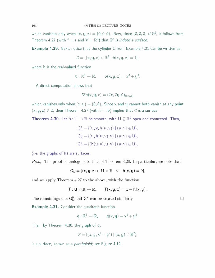
104 (MTH5113) LECTURE NOTES
which vanishes only when (x, y, z) = (0, 0, 0). Now, since (0, 0, 0) 6∈ S2, it follows fromTheorem 4.27 (with f = s and V = R3) that S2 is indeed a surface.
Example 4.29. Next, notice that the cylinder C from Example 4.21 can be written as
C = {(x, y, z) ∈ R3 | b(x, y, z) = 1},
where b is the real-valued function
b : R3 → R, b(x, y, z) = x2 + y2.
A direct computation shows that
∇b(x, y, z) = (2x, 2y, 0)(x,y,z)
which vanishes only when (x, y) = (0, 0). Since x and y cannot both vanish at any point(x, y, z) ∈ C, then Theorem 4.27 (with f = b) implies that C is a surface.
Theorem 4.30. Let h : U → R be smooth, with U ⊆ R2 open and connected. Then,
Gzh = {(u, v, h(u, v)) | (u, v) ∈ U},
Gyh = {(u, h(u, v), v) | (u, v) ∈ U},
Gxh = {(h(u, v), u, v) | (u, v) ∈ U},
(i.e. the graphs of h) are surfaces.
Proof. The proof is analogous to that of Theorem 3.28. In particular, we note that
Gzh = {(x, y, z) ∈ U× R | z− h(x, y) = 0},
and we apply Theorem 4.27 to the above, with the function
F : U× R → R, F(x, y, z) = z− h(x, y).
The remainings sets Gyh and Gx
h can be treated similarly. □
Example 4.31. Consider the quadratic function
q : R2 → R, q(x, y) = x2 + y2.
Then, by Theorem 4.30, the graph of q,
P = {(x, y, x2 + y2) | (x, y) ∈ R2},
is a surface, known as a paraboloid; see Figure 4.12.
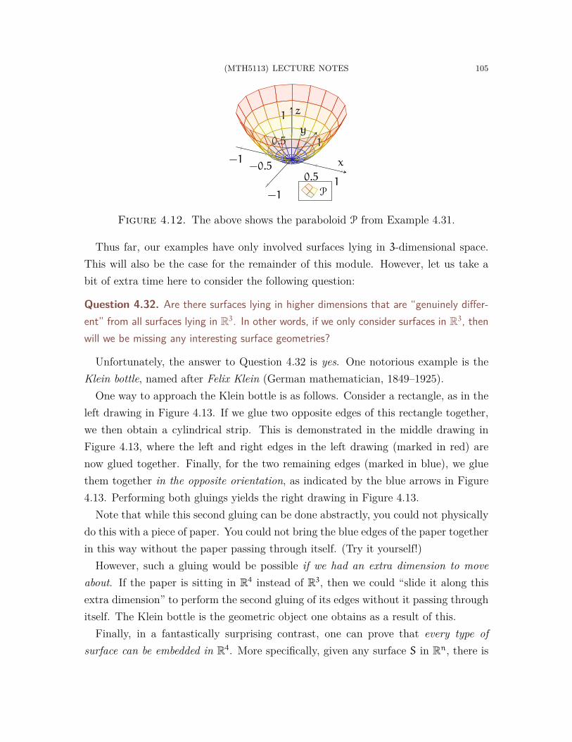
(MTH5113) LECTURE NOTES 105
−1−0.5
0.5 1
−1
10.5
1
x
y
z
P
Figure 4.12. The above shows the paraboloid P from Example 4.31.
Thus far, our examples have only involved surfaces lying in 3-dimensional space.This will also be the case for the remainder of this module. However, let us take abit of extra time here to consider the following question:
Question 4.32. Are there surfaces lying in higher dimensions that are “genuinely differ-ent” from all surfaces lying in R3. In other words, if we only consider surfaces in R3, thenwill we be missing any interesting surface geometries?
Unfortunately, the answer to Question 4.32 is yes. One notorious example is theKlein bottle, named after Felix Klein (German mathematician, 1849–1925).
One way to approach the Klein bottle is as follows. Consider a rectangle, as in theleft drawing in Figure 4.13. If we glue two opposite edges of this rectangle together,we then obtain a cylindrical strip. This is demonstrated in the middle drawing inFigure 4.13, where the left and right edges in the left drawing (marked in red) arenow glued together. Finally, for the two remaining edges (marked in blue), we gluethem together in the opposite orientation, as indicated by the blue arrows in Figure4.13. Performing both gluings yields the right drawing in Figure 4.13.
Note that while this second gluing can be done abstractly, you could not physicallydo this with a piece of paper. You could not bring the blue edges of the paper togetherin this way without the paper passing through itself. (Try it yourself!)
However, such a gluing would be possible if we had an extra dimension to moveabout. If the paper is sitting in R4 instead of R3, then we could “slide it along thisextra dimension” to perform the second gluing of its edges without it passing throughitself. The Klein bottle is the geometric object one obtains as a result of this.
Finally, in a fantastically surprising contrast, one can prove that every type ofsurface can be embedded in R4. More specifically, given any surface S in Rn, there is

106 (MTH5113) LECTURE NOTES
an “equivalent” (we avoid making this term precise here) way to also describe S as asubset of R4. Thus, if we worked instead within R4 rather than in R3, then we wouldbe able to essentially study every possible surface, including the Klein bottle.
The aforementioned result is a special case of the famous Whitney embedding the-orem, named after Hassler Whitney (American mathematician, 1907–1989).
Figure 4.13. The left drawing shows a rectangle, with each opposite pair ofedges marked with the same colour. Gluing together the red edges, with theorientations indicated by the red arrows, results in the cylindrical strip in themiddle drawing. Next, gluing the blue edges, with the opposite orientationsindicated by the blue arrows, yields the Klein bottle on the right.
4.5. Tangent Planes. Having formally defined surfaces, our next goal is to studytheir properties. Like for curves, we usually work with surfaces via their parametrisa-tions, hence we tend to deal more directly with properties of parametric surfaces. Itis then pertinent to ask whether such information is also a property of the underlyingsurface—in other words, is this property independent of parametrisation?
We now explore this question in the particular case of tangent planes of parametricsurfaces; see Definition 4.6. Before making any formal statements, let us first motivateour discussion through a concrete example involving the sphere:
Example 4.33. Consider the sphere S2 from Example 4.22,
S2 = {(x, y, z) ∈ R3 | x2 + y2 + z2 = 1},
along with the point p = (−1, 0, 0) ∈ S2. As was noted in Example 4.22, one particularparametrisation of S2 that includes p in its image is given by
ρx,− : B(0, 1) → S2, ρx,−(u, v) =(−√1− u2 − v2, u, v
).
Also, Example 4.26 provides another parametrisation of S2 containing p:
ρs,z : R× (0, π) → S2, ρs,z(u, v) = (cosu sin v, sinu sin v, cos v).
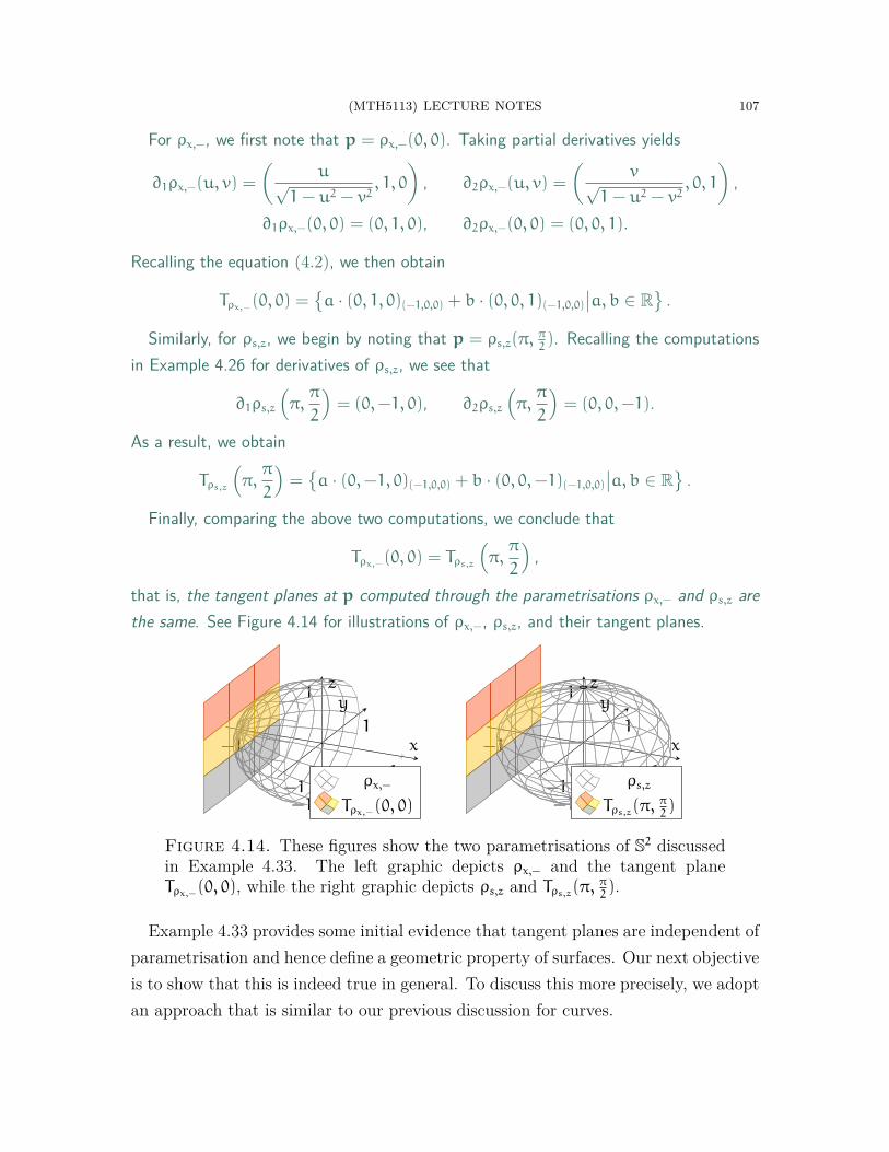
(MTH5113) LECTURE NOTES 107
For ρx,−, we first note that p = ρx,−(0, 0). Taking partial derivatives yields
∂1ρx,−(u, v) =
(u√
1− u2 − v2, 1, 0
), ∂2ρx,−(u, v) =
(v√
1− u2 − v2, 0, 1
),
∂1ρx,−(0, 0) = (0, 1, 0), ∂2ρx,−(0, 0) = (0, 0, 1).
Recalling the equation (4.2), we then obtain
Tρx,−(0, 0) ={a · (0, 1, 0)(−1,0,0) + b · (0, 0, 1)(−1,0,0)
∣∣a, b ∈ R}
.
Similarly, for ρs,z, we begin by noting that p = ρs,z(π,π2). Recalling the computations
in Example 4.26 for derivatives of ρs,z, we see that
∂1ρs,z
(π,
π
2
)= (0,−1, 0), ∂2ρs,z
(π,
π
2
)= (0, 0,−1).
As a result, we obtain
Tρs,z
(π,
π
2
)=
{a · (0,−1, 0)(−1,0,0) + b · (0, 0,−1)(−1,0,0)
∣∣a, b ∈ R}
.
Finally, comparing the above two computations, we conclude that
Tρx,−(0, 0) = Tρs,z
(π,
π
2
),
that is, the tangent planes at p computed through the parametrisations ρx,− and ρs,z arethe same. See Figure 4.14 for illustrations of ρx,−, ρs,z, and their tangent planes.
−1
1−1
1
−1
1
x
y
z
ρx,−
Tρx,−(0, 0)
−1
1−1
1
−1
1
x
y
z
ρs,z
Tρs,z(π,π2)
Figure 4.14. These figures show the two parametrisations of S2 discussedin Example 4.33. The left graphic depicts ρx,− and the tangent planeTρx,−(0, 0), while the right graphic depicts ρs,z and Tρs,z(π,
π2).
Example 4.33 provides some initial evidence that tangent planes are independent ofparametrisation and hence define a geometric property of surfaces. Our next objectiveis to show that this is indeed true in general. To discuss this more precisely, we adoptan approach that is similar to our previous discussion for curves.
108 (MTH5113) LECTURE NOTES
Definition 4.34. Let σ : U → Rn and σ : U → Rn be regular parametric surfaces. Wesay σ is a reparametrisation of σ iff there is a bijection Φ : U → U such that:
• Both Φ and its inverse Φ−1 are smooth.• The following holds for all (u, v) ∈ U:
(4.5) σ(Φ(u, v)) = σ(u, v).
In the above context, we refer to Φ as the corresponding change of variables.
Remark 4.35. Definition 4.34 is the analogue of Definition 3.12 for reparametrisations ofparametric curves. In particular, the change of variables Φ matches the parameter (u, v)for σ to the parameter (u, v) = Φ(u, v) for σ that maps to the same point.
Remark 4.36. One can again show that if σ is a reparametrisation of σ, then σ is also areparametrisation of σ. Thus, when convenient, we will write “σ and σ are reparametri-sations of each other” in the place of “σ is a reparametrisation of σ”.
The next theorem shows that reparametrisations do not alter tangent planes:
Theorem 4.37. Let σ : U → Rn and σ : U → Rn be regular parametric surfaces.Moreover, assume σ is a reparametrisation of σ, with corresponding change of variablesΦ : U → U. Then, given any (u, v) ∈ U, we have the following identity:
(4.6) Tσ(u, v) = Tσ(Φ(u, v)).
Proof. The proof is analogous to that of Theorem 3.34 for tangent lines. We let u
and v denote the individual components of Φ—that is, we set
Φ(u, v) = (u(u, v), v(u, v)).
Then, the relation (4.5) can be written as
σ(u, v) = σ(u(u, v), v(u, v)).
Using the above along with the (multivariable) chain rule, we can expand
∂1σ(u, v) = ∂1σ(u(u, v), v(u, v)) · ∂1u(u, v) + ∂2σ(u(u, v), v(u, v)) · ∂1v(u, v),
= ∂1σ(Φ(u, v)) · ∂1u(u, v) + ∂2σ(Φ(u, v)) · ∂1v(u, v),
∂2σ(u, v) = ∂1σ(u(u, v), v(u, v)) · ∂2u(u, v) + ∂2σ(u(u, v), v(u, v)) · ∂2v(u, v)
= ∂1σ(Φ(u, v)) · ∂2u(u, v) + ∂2σ(Φ(u, v)) · ∂2v(u, v).

(MTH5113) LECTURE NOTES 109
Combining (4.2) and the above, we see that
Tσ(u, v) ={a · ∂1σ(u, v)σ(u,v) + b · ∂2σ(u, v)σ(u,v)
∣∣a, b ∈ R}
={[a · ∂1u(u, v) + b · ∂2u(u, v)] · ∂1σ(Φ(u, v))σ(Φ(u,v))
+[a · ∂1v(u, v) + b · ∂2v(u, v)] · ∂2σ(Φ(u, v))σ(Φ(u,v))
∣∣a, b ∈ R}
⊆ Tσ(Φ(u, v)).
Finally, we can repeat all of the above work, but with the roles of σ and σ inter-changed; this yields the opposite relation Tσ(Φ(u, v)) ⊆ Tσ(u, v). □
In light of Theorem 4.37, we can now make sense of tangent planes to surfaces:
Definition 4.38. The tangent plane to a surface S ⊆ Rn at a point p ∈ S is defined as
(4.7) TpS = Tσ(u0, v0),
where σ : U → S is any parametrisation of S, with (u0, v0) ∈ U satisfying σ(u0, v0) = p.
Example 4.39. Recall the cylinder from Example 4.21,
C = {(x, y, z) ∈ R3 | x2 + y2 = 1}.
Let us find the tangent plane TpC, at the point p = (0, 1, 5) ∈ C.The first step is to choose a parametrisation of C which covers p. The simplest choice
is to take the parametrisation σ from Example 4.25,
σ : R2 → C, σ(u, v) = (cosu, sinu, v),
which satisfies p = σ(π2, 5). Furthermore, we can compute that
∂1σ(π2, 5)= (−1, 0, 0), ∂2σ
(π2, 5)= (0, 0, 1).
As a result, by Definition 4.38, we have
TpC = Tσ
(π2, 5)
={a · (−1, 0, 0)(0,1,5) + b · (0, 0, 1)(0,1,5)
∣∣a, b ∈ R}
.
A plot of C and TpC is found in the left drawing of Figure 4.15.
We conclude our discussion by highlighting a connection with linear algebra. As-sume the setting of Definition 4.38. Recall TpS = Tσ(u0, v0) is a 2-dimensional vectorspace, and the tangent vectors ∂1σ(u0, v0)p and ∂2σ(u0, v0)p form a basis for TpS.
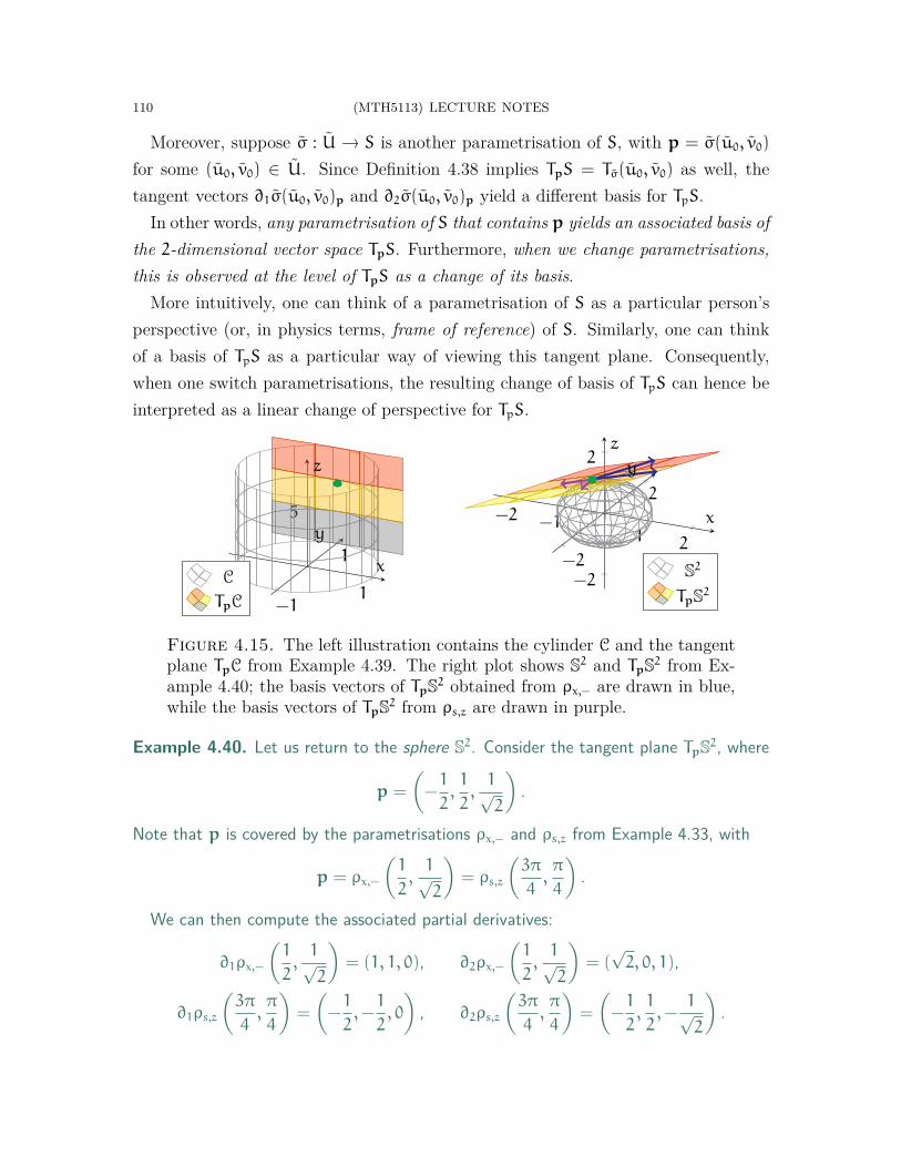
110 (MTH5113) LECTURE NOTES
Moreover, suppose σ : U → S is another parametrisation of S, with p = σ(u0, v0)
for some (u0, v0) ∈ U. Since Definition 4.38 implies TpS = Tσ(u0, v0) as well, thetangent vectors ∂1σ(u0, v0)p and ∂2σ(u0, v0)p yield a different basis for TpS.
In other words, any parametrisation of S that contains p yields an associated basis ofthe 2-dimensional vector space TpS. Furthermore, when we change parametrisations,this is observed at the level of TpS as a change of its basis.
More intuitively, one can think of a parametrisation of S as a particular person’sperspective (or, in physics terms, frame of reference) of S. Similarly, one can thinkof a basis of TpS as a particular way of viewing this tangent plane. Consequently,when one switch parametrisations, the resulting change of basis of TpS can hence beinterpreted as a linear change of perspective for TpS.
−1
1−1
1
5
x
y
z
C
TpC
−2 −11 2
−2
2
−2
2
x
y
z
S2
TpS2
Figure 4.15. The left illustration contains the cylinder C and the tangentplane TpC from Example 4.39. The right plot shows S2 and TpS2 from Ex-ample 4.40; the basis vectors of TpS2 obtained from ρx,− are drawn in blue,while the basis vectors of TpS2 from ρs,z are drawn in purple.
Example 4.40. Let us return to the sphere S2. Consider the tangent plane TpS2, where
p =
(−1
2,1
2,1√2
).
Note that p is covered by the parametrisations ρx,− and ρs,z from Example 4.33, with
p = ρx,−
(1
2,1√2
)= ρs,z
(3π
4,π
4
).
We can then compute the associated partial derivatives:
∂1ρx,−
(1
2,1√2
)= (1, 1, 0), ∂2ρx,−
(1
2,1√2
)= (
√2, 0, 1),
∂1ρs,z
(3π
4,π
4
)=
(−1
2,−
1
2, 0
), ∂2ρs,z
(3π
4,π
4
)=
(−1
2,1
2,−
1√2
).

(MTH5113) LECTURE NOTES 111
Then, the bases of TpS2 associated with ρx,− and ρs,z, respectively, are
B1 ={(1, 1, 0)p, (
√2, 0, 1)p
}, B2 =
{(−1
2,−
1
2, 0
)p
,
(−1
2,1
2,−
1√2
)p
}.
These bases are shown in the right plot of Figure 4.15 in blue and purple, respectively.Note that while B1 and B2 are clearly different, they both span the same space TpS.
4.6. Normal Vectors. In the remainder of this chapter, we will restrict ourselves tosurfaces lying only in R3 (which we have already been doing in our examples).
Let S ⊆ R3 be a surface, and let p ∈ S. Similar to our discussions for curves, thetangent plane TpS is a 2-dimensional subspace of the 3-dimensional TpR3. This leavesone remaining dimension in TpR3 normal to TpS. Since TpS captures all the directionsalong S at p, this last dimension represents the directions normal to S at p.
Again, it will be useful to pick out unit vectors from this normal dimension:
Definition 4.41. Let S ⊆ R3 be a surface, and let p ∈ S. Then, np ∈ TpR3 is a unitnormal to S at p iff np is normal to every element of TpS and |np| = 1.
−2−1
12
−2
2
−2
2
x
y
z
S2
TpS2
Figure 4.16. This is the setting of Example 4.42—the point p is drawn ingreen, while the unit normals (0, 0,±1)p are in blue and purple.
Example 4.42. Consider the sphere S2 (see Example 4.22),
S2 = {(x, y, z) ∈ R3 | x2 + y2 + z2 = 1},
along with the point p = (0, 0, 1) ∈ S2. Since p is the north pole of S2, the tangentplane TpS2 is simply a copy of the xy-plane on p:
TpS2 = {a · (1, 0, 0)p + b · (0, 1, 0)p|a, b ∈ R} .
(This can also be computed using the parametrisation ρz,+ from Example 4.22.)
112 (MTH5113) LECTURE NOTES
Thus, the z-direction is perpendicular to TpS2. In particular, the unit length arrows inthis direction are given by (0, 0,±1)p. Definition 4.41 then implies (0, 0,±1)p are bothunit normals to S2 at p = (0, 0, 1); see Figure 4.16 for an illustration of this setting.
A general observation, which you would likely find unsurprising, is that a surfacein R3 always has two unit normals at each of its points:
Theorem 4.43. Let S ⊆ R3 be a surface, and let p ∈ S. Then:• There are exactly two unit normals to S at any p.• If np is a unit normal to S at p, then so is −np.
Proof. That there are two unit normals follows from the fact that the elements ofTpR3 that are perpendicular to TpS form a 1-dimensional subspace, from which thereare exactly two elements with norm 1. For the remaining statement, we simply notethat if np satisfies the conditions of Definition 4.41, then so does −np. □
The next part of our discussion concerns a more practical question: how do wecompute unit normals? One general method is through parametrisations:
Theorem 4.44. Let S ⊆ R3 be a surface, let σ : U → S be a parametrisation of S, andfix (u0, v0) ∈ U. Then, the unit normals to S at p = σ(u0, v0) are given by
(4.8) n±p = ±
[∂1σ(u0, v0)× ∂2σ(u0, v0)
|∂1σ(u0, v0)× ∂2σ(u0, v0)|
]p
.
Proof. Recall that since σ is regular, Theorem 4.15 and Definition 4.38 imply that∂1σ(u0, v0)p and ∂2σ(u0, v0)p form a basis for the tangent plane Tσ(u0, v0) = TpS. Asa result, by Theorem 2.18, the cross product
∂1σ(u0, v0)p × ∂2σ(u0, v0)p = [∂1σ(u0, v0)× ∂2σ(u0, v0)]p
is nonzero and is normal to both of its factors, and hence to TpS. Finally, to obtainthe unit normals, we divide the above by its norm and recall Theorem 4.43. □
Example 4.45. Consider next the cylinder from Example 4.21,
C = {(x, y, z) ∈ R3 | x2 + y2 = 1}.
In addition, recall from Example 4.25 that
σ : R2 → C, σ(u, v) = (cosu, sinu, v)
is a parametrisation of C whose image is all of C.
(MTH5113) LECTURE NOTES 113
Direct computations show that for any (u, v) ∈ R2,
∂1σ(u, v) = (− sinu, cosu, 0), ∂2σ(u, v) = (0, 0, 1),
∂1σ(u, v)× ∂2σ(u, v) = (cosu, sinu, 0), |∂1σ(u, v)× ∂2σ(u, v)| = 1.
Thus, by Theorem 4.44, we conclude that for any p = σ(u0, v0) ∈ C, the tangent vectors
±[∂1σ(u0, v0)× ∂2σ(u0, v0)
|∂1σ(u0, v0)× ∂2σ(u0, v0)|
]p
= ±(cosu0, sinu0, 0)(cosu0,sinu0,v0).
are the unit normals to C at p.To state this more neatly, we set
(cosu0, sinu0, v0) = σ(u0, v0) = (x, y, z).
From the above, we conclude that the unit normals to C at (x, y, z) are
±np = ±(cosu0, sinu0, 0)(cosu0,sinu0,v0) = ±(x, y, 0)(x,y,z).
Some examples of unit normals to C are drawn in the left plot of Figure 4.17.
Furthermore, for surfaces that are level sets, in the sense of Theorem 4.27, there isa more direct method for computing their unit normals:
Theorem 4.46. Assume the setting of Theorem 4.27—let S be the surface
S = {(x, y, z) ∈ V | f(x, y, z) = c},
where V ⊆ R3 is open, c ∈ R, and f : V → R is a smooth function such that ∇f(q) isnonzero for each q ∈ S. Then, for any p ∈ S, the unit normals to S at p are given by
(4.9) n±p = ±|∇f(p)|−1 · ∇f(p).
Proof. Let σ : U → S be a parametrisation of S, and suppose σ(u0, v0) = p, with(u0, v0) ∈ U. By the definition of S, we have, for any (u, v) ∈ V , that
f(σ(u, v)) = c, ∂u[f(σ(u, v))] = 0, ∂v[f(σ(u, v))] = 0.
The second and third equations can be expanded using the chain rule:
0 = ∇f(σ(u, v)) · ∂1σ(u, v)σ(u,v), 0 = ∇f(σ(u, v)) · ∂2σ(u, v)σ(u,v).
Taking linear combinations of the above and setting (u, v) = (u0, v0) yields
0 = ∇f(p) ·[a · ∂1σ(u0, v0)σ(u0,v0) + b · ∂2σ(u0, v0)σ(u0,v0)
],
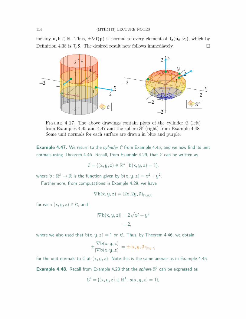
114 (MTH5113) LECTURE NOTES
for any a, b ∈ R. Thus, ±∇f(p) is normal to every element of Tσ(u0, v0), which byDefinition 4.38 is TpS. The desired result now follows immediately. □
−2−1
12
−2
−1
1
2
−2
−1
1
2
x
y
z
C
−2−1
12
−2
−1
1
2
−2
−1
1
2
x
y
z
S2
Figure 4.17. The above drawings contain plots of the cylinder C (left)from Examples 4.45 and 4.47 and the sphere S2 (right) from Example 4.48.Some unit normals for each surface are drawn in blue and purple.
Example 4.47. We return to the cylinder C from Example 4.45, and we now find its unitnormals using Theorem 4.46. Recall, from Example 4.29, that C can be written as
C = {(x, y, z) ∈ R3 | b(x, y, z) = 1},
where b : R3 → R is the function given by b(x, y, z) = x2 + y2.Furthermore, from computations in Example 4.29, we have
∇b(x, y, z) = (2x, 2y, 0)(x,y,z)
for each (x, y, z) ∈ C, and
|∇b(x, y, z)| = 2√x2 + y2
= 2,
where we also used that b(x, y, z) = 1 on C. Thus, by Theorem 4.46, we obtain
± ∇b(x, y, z)
|∇b(x, y, z)|= ±(x, y, 0)(x,y,z)
for the unit normals to C at (x, y, z). Note this is the same answer as in Example 4.45.
Example 4.48. Recall from Example 4.28 that the sphere S2 can be expressed as
S2 = {(x, y, z) ∈ R3 | s(x, y, z) = 1},

(MTH5113) LECTURE NOTES 115
where the function s : R3 → R is given by s(x, y, z) = x2 + y2 + z2. Furthermore, forany (x, y, z) ∈ S2, the gradient of s at (x, y, z) satisfies
∇s(x, y, z) = (2x, 2y, 2z)(x,y,z), |∇s(x, y, z)| = 2.
Thus, by Theorem 4.46, the unit normals to S2 at (x, y, z) are
± ∇s(x, y, z)
|∇s(x, y, z)|= ±(x, y, z)(x,y,z).
In other words, the unit normals of S2 at any of its points p is simply ±pp. See the rightplot within Figure 4.17 for some illustrations of unit normals of S2.
A B
S
TpS A B
S
TpS
Figure 4.18. The left illustration shows the two sides (labelled “A” and“B”) of a tangent plane TpS. In the right graphic, two unit normals (in blueand purple) extending from TpS are added; the blue normal represents side“A”, while the purple normal represents side “B”.
Finally, we relate unit normals to a basic property of planes—that they are “two-sided”. Intuitively, we can think of a plane as a flat (infinite) piece of paper. Just asthe paper has a front and a back side, an abstract plane also has two faces.
Now, for a surface S ⊆ R3, we can think of a tangent plane TpS as splitting TpR3 intotwo halves—with one side of TpS facing one of the halves of TpR3, and the other side ofTpS facing the other half; see the left part of Figure 4.18. One precise way to capturethese “sides” of TpS is through unit normals. In particular, we simply associate aunit normal np with the side of TpS facing the direction that np is pointing. This isillustrated in the right part of Figure 4.18.
Remark 4.49. In fact, even for surfaces in higher dimensions (S ⊆ Rn), one can stillmake sense of their tangent planes being “two-sided”. However, this property is trickierto capture mathematically, hence we avoid discussing this here.
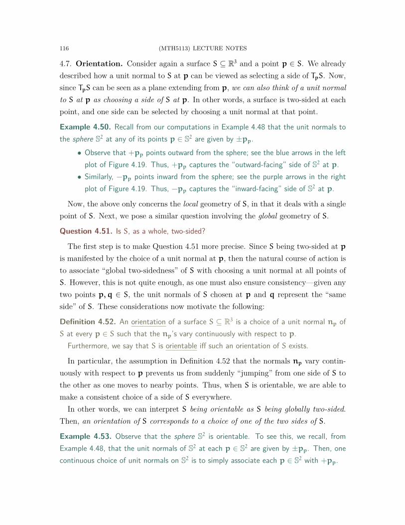
116 (MTH5113) LECTURE NOTES
4.7. Orientation. Consider again a surface S ⊆ R3 and a point p ∈ S. We alreadydescribed how a unit normal to S at p can be viewed as selecting a side of TpS. Now,since TpS can be seen as a plane extending from p, we can also think of a unit normalto S at p as choosing a side of S at p. In other words, a surface is two-sided at eachpoint, and one side can be selected by choosing a unit normal at that point.
Example 4.50. Recall from our computations in Example 4.48 that the unit normals tothe sphere S2 at any of its points p ∈ S2 are given by ±pp.
• Observe that +pp points outward from the sphere; see the blue arrows in the leftplot of Figure 4.19. Thus, +pp captures the “outward-facing” side of S2 at p.
• Similarly, −pp points inward from the sphere; see the purple arrows in the rightplot of Figure 4.19. Thus, −pp captures the “inward-facing” side of S2 at p.
Now, the above only concerns the local geometry of S, in that it deals with a singlepoint of S. Next, we pose a similar question involving the global geometry of S.
Question 4.51. Is S, as a whole, two-sided?
The first step is to make Question 4.51 more precise. Since S being two-sided at pis manifested by the choice of a unit normal at p, then the natural course of action isto associate “global two-sidedness” of S with choosing a unit normal at all points ofS. However, this is not quite enough, as one must also ensure consistency—given anytwo points p,q ∈ S, the unit normals of S chosen at p and q represent the “sameside” of S. These considerations now motivate the following:
Definition 4.52. An orientation of a surface S ⊆ R3 is a choice of a unit normal np ofS at every p ∈ S such that the np’s vary continuously with respect to p.
Furthermore, we say that S is orientable iff such an orientation of S exists.
In particular, the assumption in Definition 4.52 that the normals np vary contin-uously with respect to p prevents us from suddenly “jumping” from one side of S tothe other as one moves to nearby points. Thus, when S is orientable, we are able tomake a consistent choice of a side of S everywhere.
In other words, we can interpret S being orientable as S being globally two-sided.Then, an orientation of S corresponds to a choice of one of the two sides of S.
Example 4.53. Observe that the sphere S2 is orientable. To see this, we recall, fromExample 4.48, that the unit normals of S2 at each p ∈ S2 are given by ±pp. Then, onecontinuous choice of unit normals on S2 is to simply associate each p ∈ S2 with +pp.
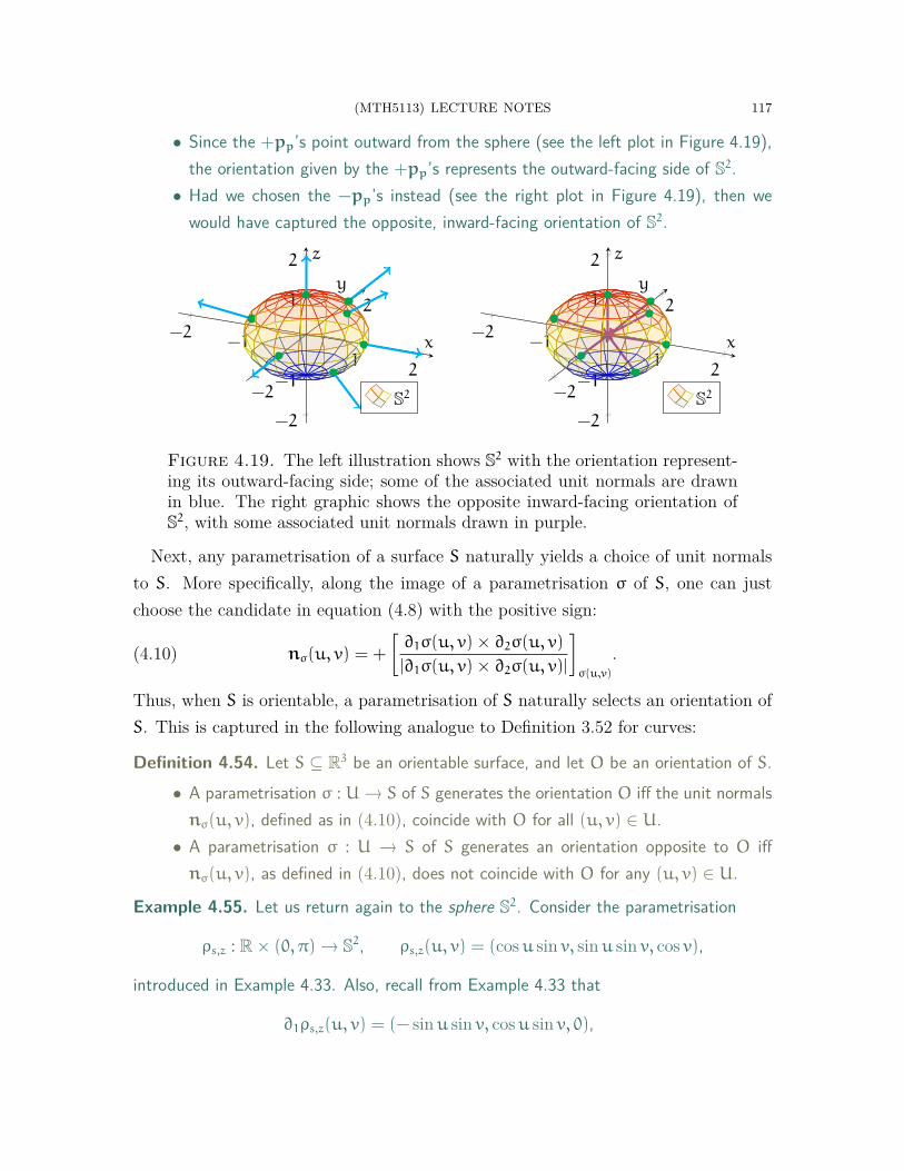
(MTH5113) LECTURE NOTES 117
• Since the +pp’s point outward from the sphere (see the left plot in Figure 4.19),the orientation given by the +pp’s represents the outward-facing side of S2.
• Had we chosen the −pp’s instead (see the right plot in Figure 4.19), then wewould have captured the opposite, inward-facing orientation of S2.
−2−1
12
−2
2
−2
−1
1
2
x
y
z
S2
−2−1
12
−2
2
−2
−1
1
2
x
y
z
S2
Figure 4.19. The left illustration shows S2 with the orientation represent-ing its outward-facing side; some of the associated unit normals are drawnin blue. The right graphic shows the opposite inward-facing orientation ofS2, with some associated unit normals drawn in purple.
Next, any parametrisation of a surface S naturally yields a choice of unit normalsto S. More specifically, along the image of a parametrisation σ of S, one can justchoose the candidate in equation (4.8) with the positive sign:
(4.10) nσ(u, v) = +
[∂1σ(u, v)× ∂2σ(u, v)
|∂1σ(u, v)× ∂2σ(u, v)|
]σ(u,v)
.
Thus, when S is orientable, a parametrisation of S naturally selects an orientation ofS. This is captured in the following analogue to Definition 3.52 for curves:
Definition 4.54. Let S ⊆ R3 be an orientable surface, and let O be an orientation of S.• A parametrisation σ : U → S of S generates the orientation O iff the unit normalsnσ(u, v), defined as in (4.10), coincide with O for all (u, v) ∈ U.
• A parametrisation σ : U → S of S generates an orientation opposite to O iffnσ(u, v), as defined in (4.10), does not coincide with O for any (u, v) ∈ U.
Example 4.55. Let us return again to the sphere S2. Consider the parametrisation
ρs,z : R× (0, π) → S2, ρs,z(u, v) = (cosu sin v, sinu sin v, cos v),
introduced in Example 4.33. Also, recall from Example 4.33 that
∂1ρs,z(u, v) = (− sinu sin v, cosu sin v, 0),

118 (MTH5113) LECTURE NOTES
∂2ρs,z(u, v) = (cosu cos v, sinu cos v,− sin v).
Next, taking a cross product of the above vectors, we see that
∂1ρs,z(u, v)× ∂2ρs,z(u, v) = (− cosu sin2 v,− sinu sin2 v,− cos v sin v)
= − sin v · ρs,z(u, v),
|∂1ρs,z(u, v)× ∂2ρs,z(u, v)| = sin v.
In particular, the formula (4.10), with ρs,z in the place of σ, selects the unit normals
nρs,z(u, v) = +
[∂1ρs,z(u, v)× ∂2ρs,z(u, v)
|∂1ρs,z(u, v)× ∂2ρs,z(u, v)|
]ρs,z(u,v)
= −ρs,z(u, v)ρs,z(u,v),
for any (u, v) ∈ R × (0, π). More explicitly, for any p = ρs,z(u, v), the parametrisationρs,z selects the inward-pointing unit normal −pp. Therefore, according to Definition 4.54,the parametrisation ρs,z generates the inward-facing orientation of S2.
In contrast, consider instead the parametrisation
ρs,z : (0, π)× R → S2, ρs,z(u, v) = (cos v sinu, sin v sinu, cosu),
that is, ρs,z with the roles of u and v interchanged. Similar computations then yield
nρs,z(u, v) = +
[∂1ρs,z(u, v)× ∂2ρs,z(u, v)
|∂1ρs,z(u, v)× ∂2ρs,z(u, v)|
]ρs,z(u,v)
= +ρs,z(u, v)ρs,z(u,v),
hence ρs,z generates the outward-facing orientation of S2.
The following definition formalises the idea of a “surface with a chosen side”:
Definition 4.56. An oriented surface is a surface S along with a chosen orientation of S.
Finally, we look at an example of a non-orientable surface: the Möbius strip. Onesimple way to construct this Möbius strip is to take a rectangle and glue two of itsopposite edges together “in reverse order”; see Figure 4.20. To try this yourself, takea thin strip of paper, twist it halfway, and then tape the two ends together.
Intuitively, the Möbius strip is not orientable since it has only one side, rather thantwo. Although any small portion of the strip is two sided, at the global scale, the twosides blend into each other whenever one goes a full revolution around the strip.

(MTH5113) LECTURE NOTES 119
Figure 4.20. These drawings demonstrate how the Möbius strip can beconstructed by gluing together two opposite edges of a rectangle.
Example 4.57. Consider the parametric surface σ : (−1, 1)× R → R3 defined by
σ(u, v) =((
1−u
2sin v
2
)cos v,
(1−
u
2sin v
2
)sin v,
u
2cos v
2
),
whose image is plotted in the left side of Figure 4.21. The Möbius strip can then be moreconcretely described as the image M of σ. (With some effort, one can in fact show thatM satisfies the hypotheses of Definition 4.20.)
−1
1−1
1
−1
1
x
y
z
M
−2−1
12
−2
2
−2
−1
1
2
x
y
z
M
Figure 4.21. The left plot contains the image M of the parametric surfaceσ from Example 4.57, representing the Möbius strip. The right plot demon-strates why M fails to be orientable—any choice of unit normals along thestrip must fail to vary continuously at some point.
We can also give an informal argument for why the Möbius strip fails to be ori-entable. Consider the strip M in the right plot of Figure 4.21, and consider the blueunit normal np at the point p ∈ M (in green). Let us now try to construct from np
a continuous choice of unit normals along all of M.As we traverse (anticlockwise) along the red path on M, we see that our hand is
forced. The unit normals are determined by the requirement that they vary continu-ously along this red path; some of these unit normals are drawn in purple in the rightside of Figure 4.21. The problem arises once we travel a full lap around M alongthe red path. In particular, once we return to p, the unit normal that we are forced
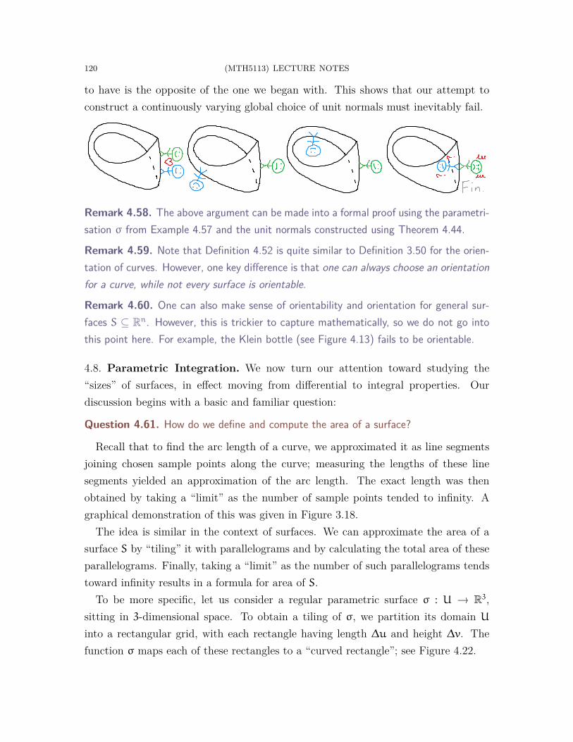
120 (MTH5113) LECTURE NOTES
to have is the opposite of the one we began with. This shows that our attempt toconstruct a continuously varying global choice of unit normals must inevitably fail.
Remark 4.58. The above argument can be made into a formal proof using the parametri-sation σ from Example 4.57 and the unit normals constructed using Theorem 4.44.
Remark 4.59. Note that Definition 4.52 is quite similar to Definition 3.50 for the orien-tation of curves. However, one key difference is that one can always choose an orientationfor a curve, while not every surface is orientable.
Remark 4.60. One can also make sense of orientability and orientation for general sur-faces S ⊆ Rn. However, this is trickier to capture mathematically, so we do not go intothis point here. For example, the Klein bottle (see Figure 4.13) fails to be orientable.
4.8. Parametric Integration. We now turn our attention toward studying the“sizes” of surfaces, in effect moving from differential to integral properties. Ourdiscussion begins with a basic and familiar question:
Question 4.61. How do we define and compute the area of a surface?
Recall that to find the arc length of a curve, we approximated it as line segmentsjoining chosen sample points along the curve; measuring the lengths of these linesegments yielded an approximation of the arc length. The exact length was thenobtained by taking a “limit” as the number of sample points tended to infinity. Agraphical demonstration of this was given in Figure 3.18.
The idea is similar in the context of surfaces. We can approximate the area of asurface S by “tiling” it with parallelograms and by calculating the total area of theseparallelograms. Finally, taking a “limit” as the number of such parallelograms tendstoward infinity results in a formula for area of S.
To be more specific, let us consider a regular parametric surface σ : U → R3,sitting in 3-dimensional space. To obtain a tiling of σ, we partition its domain U
into a rectangular grid, with each rectangle having length ∆u and height ∆v. Thefunction σ maps each of these rectangles to a “curved rectangle”; see Figure 4.22.
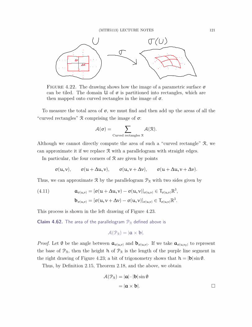
(MTH5113) LECTURE NOTES 121
Figure 4.22. The drawing shows how the image of a parametric surface σ
can be tiled. The domain U of σ is partitioned into rectangles, which arethen mapped onto curved rectangles in the image of σ.
To measure the total area of σ, we must find and then add up the areas of all the“curved rectangles” R comprising the image of σ:
A(σ) =∑
Curved rectangles R
A(R).
Although we cannot directly compute the area of such a “curved rectangle” R, wecan approximate it if we replace R with a parallelogram with straight edges.
In particular, the four corners of R are given by points
σ(u, v), σ(u+ ∆u, v), σ(u, v+ ∆v), σ(u+ ∆u, v+ ∆v).
Thus, we can approximate R by the parallelogram PR with two sides given by
aσ(u,v) = [σ(u+ ∆u, v) − σ(u, v)]σ(u,v) ∈ Tσ(u,v)R3,(4.11)
bσ(u,v) = [σ(u, v+ ∆v) − σ(u, v)]σ(u,v) ∈ Tσ(u,v)R3.
This process is shown in the left drawing of Figure 4.23.
Claim 4.62. The area of the parallelogram PR defined above is
A(PR) = |a× b|.
Proof. Let θ be the angle between aσ(u,v) and bσ(u,v). If we take aσ(u,v0) to representthe base of PR, then the height h of PR is the length of the purple line segment inthe right drawing of Figure 4.23; a bit of trigonometry shows that h = |b| sin θ.
Thus, by Definition 2.15, Theorem 2.18, and the above, we obtain
A(PR) = |a| · |b| sin θ
= |a× b|. □
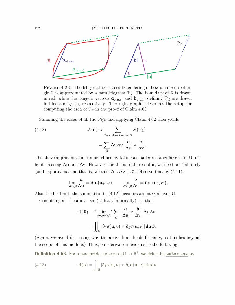
122 (MTH5113) LECTURE NOTES
R
aσ(u,v)
bσ(u,v)
PR
|a|
|b| h
θ
Figure 4.23. The left graphic is a crude rendering of how a curved rectan-gle R is approximated by a parallelogram PR. The boundary of R is drawnin red, while the tangent vectors aσ(u,v) and bσ(u,v) defining PR are drawnin blue and green, respectively. The right graphic describes the setup forcomputing the area of PR in the proof of Claim 4.62.
Summing the areas of all the PR’s and applying Claim 4.62 then yields
A(σ) ≈∑
Curved rectangles R
A(PR)(4.12)
=∑R
∆u∆v
∣∣∣∣ a∆u × b
∆v
∣∣∣∣ .The above approximation can be refined by taking a smaller rectangular grid in U, i.e.by decreasing ∆u and ∆v. However, for the actual area of σ, we need an “infinitelygood” approximation, that is, we take ∆u,∆v ↘ 0. Observe that by (4.11),
lim∆u↘0
a
∆u= ∂1σ(u0, v0), lim
∆v↘0
b
∆v= ∂2σ(u0, v0).
Also, in this limit, the summation in (4.12) becomes an integral over U.Combining all the above, we (at least informally) see that
A(R) = ‘‘ lim∆u,∆v↘0
"∑R
∣∣∣∣ a∆u × b
∆v
∣∣∣∣∆u∆v=
∫∫U
|∂1σ(u, v)× ∂2σ(u, v)|dudv.
(Again, we avoid discussing why the above limit holds formally, as this lies beyondthe scope of this module.) Thus, our derivation leads us to the following:
Definition 4.63. For a parametric surface σ : U → R3, we define its surface area as
(4.13) A(σ) =
∫∫U
|∂1σ(u, v)× ∂2σ(u, v)|dudv.
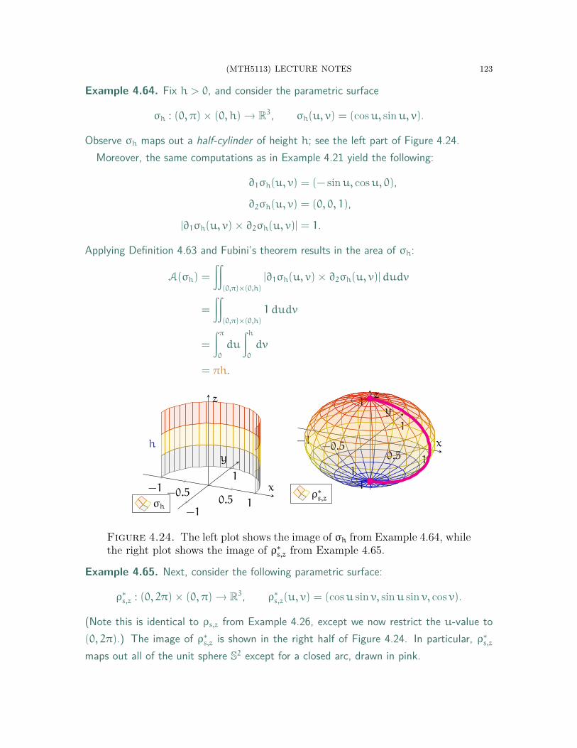
(MTH5113) LECTURE NOTES 123
Example 4.64. Fix h > 0, and consider the parametric surface
σh : (0, π)× (0, h) → R3, σh(u, v) = (cosu, sinu, v).
Observe σh maps out a half-cylinder of height h; see the left part of Figure 4.24.Moreover, the same computations as in Example 4.21 yield the following:
∂1σh(u, v) = (− sinu, cosu, 0),
∂2σh(u, v) = (0, 0, 1),
|∂1σh(u, v)× ∂2σh(u, v)| = 1.
Applying Definition 4.63 and Fubini’s theorem results in the area of σh:
A(σh) =
∫∫(0,π)×(0,h)
|∂1σh(u, v)× ∂2σh(u, v)|dudv
=
∫∫(0,π)×(0,h)
1 dudv
=
∫π
0
du
∫h
0
dv
= πh.
−1 −0.50.5 1
−1
1
h
x
y
z
σh
−1−0.5
0.5 1−1
1
−1
1
x
y
z
ρ∗s,z
Figure 4.24. The left plot shows the image of σh from Example 4.64, whilethe right plot shows the image of ρ∗
s,z from Example 4.65.
Example 4.65. Next, consider the following parametric surface:
ρ∗s,z : (0, 2π)× (0, π) → R3, ρ∗
s,z(u, v) = (cosu sin v, sinu sin v, cos v).
(Note this is identical to ρs,z from Example 4.26, except we now restrict the u-value to(0, 2π).) The image of ρ∗
s,z is shown in the right half of Figure 4.24. In particular, ρ∗s,z
maps out all of the unit sphere S2 except for a closed arc, drawn in pink.
124 (MTH5113) LECTURE NOTES
Now, from computations similar to those in Example 4.26, we see that
|∂1ρ∗s,z(u, v)× ∂2ρ
∗s,z(u, v)| = sin v, (u, v) ∈ (0, 2π)× (0, π).
Thus, by Definition 4.63 and Fubini’s theorem, the area of ρ∗s,z is
A(ρ∗s,z) =
∫∫(0,2π)×(0,π)
|∂1ρ∗s,z(u, v)× ∂2ρ
∗s,z(u, v)|dudv
=
∫ 2π
0
du
∫π
0
sin v dv
= 4π.
Since the image of ρ∗s,z differs from the sphere S2 only by a 1-dimensional arc (which
one thinks should have negligible area), this suggests (as expected) that the surface areaof S2 itself should also be 4π. We will revisit this point more formally later on.
Remark 4.66. With a bit of algebra, one can show the following holds for any a,b ∈ R3:
|a× b|2 =
∣∣∣∣∣det
[a · a a · bb · a b · b
]∣∣∣∣∣Thus, assuming the setting of Definition 4.63, and setting a and b to be the values of∂1σ and ∂2σ, respectively, we obtain an alternative formula for surface area:
(4.14) A(σ) =
∫∫U
√F(u, v)dudv, F =
∣∣∣∣∣det
[∂1σ · ∂1σ ∂1σ · ∂2σ
∂2σ · ∂1σ ∂2σ · ∂2σ
]∣∣∣∣∣ .While (4.14) is no simpler than (4.13), it does have the advantage that the quantity
F(u, v) makes sense when σ takes values in any Rn, and not only R3. Thus, (4.14) givesa sensible definition of surface area for parametric surfaces in all dimensions.
4.9. Surface Integrals. Having defined the area of parametric surfaces, the nextaim is to extend our understanding to “weighted” areas. Similar to our discussionsfor curves, we will achieve this by constructing a theory of surface integration.
Consider the area formula (4.13) for a parametric surface σ. There, the integrand
(4.15) |∂1σ(u, v)× ∂2σ(u, v)|
represents the area of an “infinitesimal” parallelogram at the point σ(u, v). Thus, ifwe wish to add a weight F to the area (4.13), then the factor (4.15) should be pairedwith F, applied to the same point σ(u, v). These considerations lead to the following:
(MTH5113) LECTURE NOTES 125
Definition 4.67. Let σ : U → R3 be a parametric surface, and let F be a real-valuedfunction defined on the image of σ. We define the surface integral of F over σ by
(4.16)∫∫
σ
F dA =
∫∫U
F(σ(u, v))|∂1σ(u, v)× ∂2σ(u, v)|dudv.
Example 4.68. Consider the half-cylinder from Example 4.64, but with h = 1:
σ : (0, π)× (0, 1) → R3, σ(u, v) = (cosu, sinu, v).
(See the left part of Figure 4.25.) Let us integrate over σ the function
G : R3 → R, G(x, y, z) = x+ y+ z.
First, recall from the computations in Example 4.64 that
|∂1σ(u, v)× ∂2σ(u, v)| = 1, (u, v) ∈ (0, π)× (0, 1).
In addition, observe that for the same values of (u, v),
G(σ(u, v)) = G(cosu, sinu, v)
= cosu+ sinu+ v.
Therefore, applying Definition 4.67 and Fubini’s theorem, we conclude that∫∫σ
GdA =
∫(0,π)×(0,1)
G(σ(u, v))|∂1σ(u, v)× ∂2σ(u, v)|dudv
=
∫ 1
0
[∫π
0
(cosu+ sinu+ v) · 1 · du]dv
=
∫ 1
0
(0+ 2+ πv)dv
= 2+π
2.
Example 4.69. Consider the following portion of a parametric paraboloid:
P : (0, 1)× (0, 1) → R3, P(u, v) = (u, v, u2 + v2).
(See the right side of Figure 4.25.) Observe that a direct computation yields
|∂1P(u, v)× ∂2P(u, v)| = |(1, 0, 2u)× (0, 1, 2v)|
=√
1+ 4u2 + 4v2,
for any parameters (u, v) ∈ (0, 1)× (0, 1).
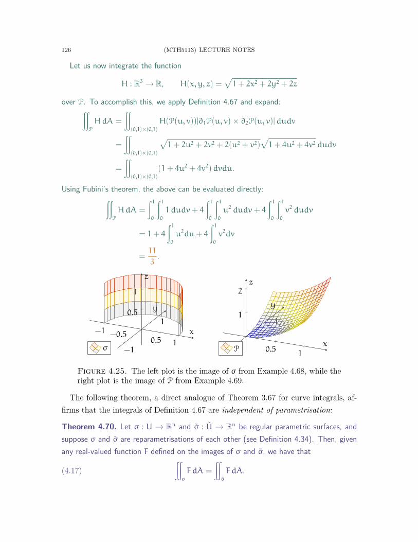
126 (MTH5113) LECTURE NOTES
Let us now integrate the function
H : R3 → R, H(x, y, z) =√
1+ 2x2 + 2y2 + 2z
over P. To accomplish this, we apply Definition 4.67 and expand:∫∫P
HdA =
∫∫(0,1)×(0,1)
H(P(u, v))|∂1P(u, v)× ∂2P(u, v)|dudv
=
∫∫(0,1)×(0,1)
√1+ 2u2 + 2v2 + 2(u2 + v2)
√1+ 4u2 + 4v2 dudv
=
∫∫(0,1)×(0,1)
(1+ 4u2 + 4v2)dvdu.
Using Fubini’s theorem, the above can be evaluated directly:∫∫P
HdA =
∫ 1
0
∫ 1
0
1 dudv+ 4
∫ 1
0
∫ 1
0
u2 dudv+ 4
∫ 1
0
∫ 1
0
v2 dudv
= 1+ 4
∫ 1
0
u2du+ 4
∫ 1
0
v2dv
=11
3.
−1 −0.50.5 1
−1
10.5
1
x
y
z
σ 0.51
11
2
x
y
z
P
Figure 4.25. The left plot is the image of σ from Example 4.68, while theright plot is the image of P from Example 4.69.
The following theorem, a direct analogue of Theorem 3.67 for curve integrals, af-firms that the integrals of Definition 4.67 are independent of parametrisation:
Theorem 4.70. Let σ : U → Rn and σ : U → Rn be regular parametric surfaces, andsuppose σ and σ are reparametrisations of each other (see Definition 4.34). Then, givenany real-valued function F defined on the images of σ and σ, we have that
(4.17)∫∫
σ
F dA =
∫∫σ
F dA.

(MTH5113) LECTURE NOTES 127
In particular, σ and σ have the same surface area: A(σ) = A(σ).
Proof. We give a brief sketch of the proof here, though we omit many computationaldetails. Let Φ be the change of variables for σ and σ, for which the following holds:
σ(u, v) = σ(Φ(u, v)), (u, v) ∈ U.
The key step is to substitute (u, v) = Φ(u, v) into the right-hand side of (4.16):∫∫σ
F dA =
∫∫U
F(σ(Φ(u, v)))|∂1σ(u, v)× ∂2σ(u, v)|dudv
=
∫∫U
F(σ(u, v)) |∂1σ(Φ−1(u, v))× ∂2σ(Φ
−1(u, v))| |JΦ(u, v)|dudv.
Here, JΦ denotes the Jacobian determinant associated with this change of variables.The main observation—also the main computation of the proof—is the identity
(4.18) |∂1σ(Φ−1(u, v))× ∂2σ(Φ
−1(u, v))| |JΦ(u, v)| = |∂1σ(u, v)× ∂2σ(u, v)|.
(In particular, slightly annoying calculuations using the chain rule yield that
|∂1σ(Φ−1(u, v))× ∂2σ(Φ
−1(u, v))|, |∂1σ(u, v)× ∂2σ(u, v)|
differ by a factor that is the determinant of a matrix. In addition, this is preciselythe matrix found in the Jacobian JΦ, and hence the identity (4.18) follows.)
Combining all the above and recalling again (4.16), we conclude that∫∫σ
F dA =
∫∫U
F(σ(u, v))|∂1σ(u, v)× ∂2σ(u, v)|dudv
=
∫∫σ
F dA,
which is (4.17). Finally, taking F ≡ 1 in (4.17) yields A(σ) = A(σ). □
In particular, we can use Definitions 4.63 and 4.67 to make sense of areas of surfacesand integrals over surfaces, i.e. both are geometric properties of surfaces.
Definition 4.71. Let S ⊆ R3 be a surface, and let σ : U → S be an injective parametri-sation of S, whose image differs from S by only a finite number of points and curves.
• For any real-valued function F on S, we define its surface integral over S by
(4.19)∫∫
S
F dA =
∫∫σ
F dA.
• Moreover, we define the surface area of S by A(S) = A(σ).
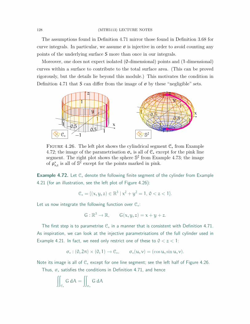
128 (MTH5113) LECTURE NOTES
The assumptions found in Definition 4.71 mirror those found in Definition 3.68 forcurve integrals. In particular, we assume σ is injective in order to avoid counting anypoints of the underlying surface S more than once in our integrals.
Moreover, one does not expect isolated (0-dimensional) points and (1-dimensional)curves within a surface to contribute to the total surface area. (This can be provedrigorously, but the details lie beyond this module.) This motivates the condition inDefinition 4.71 that S can differ from the image of σ by these “negligible” sets.
−1 −0.50.5 1
−1
1
1
x
y
z
C∗
−1 −0.50.5 1
−1
1
−1
1
x
y
z
S2
Figure 4.26. The left plot shows the cylindrical segment C∗ from Example4.72; the image of the parametrisation σ∗ is all of C∗ except for the pink linesegment. The right plot shows the sphere S2 from Example 4.73; the imageof ρ∗
s,z is all of S2 except for the points marked in pink.
Example 4.72. Let C∗ denote the following finite segment of the cylinder from Example4.21 (for an illustration, see the left plot of Figure 4.26):
C∗ = {(x, y, z) ∈ R3 | x2 + y2 = 1, 0 < z < 1}.
Let us now integrate the following function over C∗:
G : R3 → R, G(x, y, z) = x+ y+ z.
The first step is to parametrise C∗ in a manner that is consistent with Definition 4.71.As inspiration, we can look at the injective parametrisations of the full cylinder used inExample 4.21. In fact, we need only restrict one of these to 0 < z < 1:
σ∗ : (0, 2π)× (0, 1) → C∗, σ∗(u, v) = (cosu, sinu, v).
Note its image is all of C∗ except for one line segment; see the left half of Figure 4.26.Thus, σ∗ satisfies the conditions in Definition 4.71, and hence∫∫
C∗
GdA =
∫∫σ∗
GdA
(MTH5113) LECTURE NOTES 129
=
∫∫(0,2π)×(0,1)
G(σ∗(u, v))|∂1σ∗(u, v)× ∂2σ∗(u, v)|dudv.
The right-hand side can now be computed in the same manner as in Example 4.68:∫∫C∗
GdA =
∫ 1
0
[∫ 2π
0
(cosu+ sinu+ v)1 du
]dv
= 2π
∫ 1
0
v dv
= π.
Example 4.73. Next, consider the sphere S2, and recall the parametrisation
ρ∗s,z : (0, 2π)× (0, π) → S2, ρ∗
s,z(u, v) = (cosu sin v, sinu sin v, cos v)
of S2 from Example 4.65. Note the domain restrictions u ∈ (0, 2π) and v ∈ (0, π) implythat ρ∗
s,z is injective. Moreover, the image of ρ∗s,z is all of S2, except for the poles (0, 0,±1)
and a semicircle—see the pink arc in the right plot of Figure 4.26.As a result, the parametrisation ρ∗
s,z satisfies the assumptions of Definition 4.71. Fur-thermore, recall from Example 4.65 that the area of ρ∗
s,z is 4π. Thus, by Definition 4.71,we obtain the standard formula for the surface area of a unit sphere:
A(S2) = A(ρ∗s,z) = 4π.
4.10. Integration of Vector Fields. In this final section, we discuss a differentnotion of surface integration, in which the integrand is a vector field.
The main motivation for this comes from the notion of flux in physics, whichroughly quantifies a “rate of flow through a surface”. The term “flow” could referto many different phenomena, including the motion of a fluid or an electromagneticforce. Mathematically, such a flow is expressed using a vector field F. In the case offluids, the arrow F(p) represents the velocity of the fluid at the position p.
The flux of F through a surface S should measure “the total amount that the arrowsof F pass through S”. More specifically, we must keep in mind the following:
• If the values of F lie tangent to S (that is, the fluid flows along but not throughS), then one should measure zero flux. This is shown in the left drawing ofFigure 4.27. Thus, only the component of F that is normal to S matters.
• Moreover, when F has a component normal to S, we also want to measurewhich way F passes through S. (See the middle and right drawings of Figure

130 (MTH5113) LECTURE NOTES
4.27, which show two vector fields flowing through S in opposite directions.)To achieve this, we will associate one direction through S with positive flux,and the other direction with negative flux.
Figure 4.27. In the left drawing, the vector field F is tangent to the surfaceS; in this case, there is zero flux. On the other hand, in the middle and rightdrawings, F is normal to S, but pointing in opposite directions; the flux isnonzero in both cases, however they will have opposite signs.
However, the above discussion leaves open a key question: which of the two direc-tions through S should correspond to positive flux? In general, both directions areequally plausible, thus we will have to make an extra choice.
Now, this choice of a direction through S is connected to the choice of unit normalsto S. In particular, if F(p) points in the same direction as the chosen unit normal np
at p, then the flow can be considered “positive”. On the other hand, if F(p) pointsin the opposite direction as np, then the flow is deemed “negative”.
Notice the above can be very conveniently captured by the dot product F(p) · np.Indeed, this is precisely the component of F in the np-direction, and it is positive ifand only if F is pointing in the same normal direction as np.
Moreover, by Definition 4.52, such a choice of unit normals n is determined by anorientation of S. Thus, we can make sense of the flux through S only after we havechosen an orientation of S, which gives the direction corresponding to positive flux.For example, in Figure 4.27, if we assign the “upward-facing” orientation of S, thenthe middle and right drawings demonstrate positive and negative flux, respectively.
Combining all the above, we arrive at our formal notion of “flux integral”:
Definition 4.74. Let S ⊆ R3 be an oriented surface, and let F be a vector field on asubset of R3 containing S. Then, we define the surface integral of F over S by
(4.20)∫∫
S
F · dA =
∫∫S
(F · n)dA,
(MTH5113) LECTURE NOTES 131
where n denotes the unit normals of S in the direction specified by the orientation of S,and where the integral on the right-hand side is defined as in (4.19).
Remark 4.75. Note in particular that if one reverses the orientation of S, then the onlychange to the right-hand side of (4.20) is that n is replaced by −n. Therefore, if S∗
denotes the same surface S, but with the opposite orientation, then∫∫S∗F · dA = −
∫∫S
F · dA.
Remark 4.76. Definition 4.74 is similar to Definition 3.75 for curve integrals of vectorfields. However, one key difference is that Definition 4.74 measures our vector field withrespect to the unit normal, whereas Definition 3.75 uses the unit tangent.
The next task is to find a practical method for computing surface integrals ofvector fields. The subsequent theorem, which is an analogue of Theorem 3.77 forcurve integrals, provides a convenient formula using parametrisations:
Theorem 4.77. Let S, F be as in Definition 4.74, and let σ : U → S be an injectiveparametrisation of S, whose image differs from S by a finite collection of points and curves.
• If σ generates the orientation of S, then
(4.21)∫∫
S
F · dA = +
∫∫U
{F(σ(u, v)) · [∂1σ(u, v)× ∂2σ(u, v)]σ(u,v)
}dudv.
• If σ generates the orientation opposite to that of S, then
(4.22)∫∫
S
F · dA = −
∫∫U
{F(σ(u, v)) · [∂1σ(u, v)× ∂2σ(u, v)]σ(u,v)
}dudv.
Proof. First, if σ generates the orientation of S, then Definition 4.54 implies that thechosen unit normal to S at σ(u, v), for any (u, v) ∈ U, is
nσ(u,v) = +
[w(u, v)
|w(u, v)|
]σ(u,v)
, w(u, v) = ∂1σ(u, v)× ∂2σ(u, v).
Thus, using Definitions 4.67, 4.71, and 4.74, we conclude that∫∫S
F · dA =
∫∫U
{F(σ(u, v)) ·
[w(u, v)
|w(u, v)|
]σ(u,v)
}|w(u, v)|dudv
=
∫∫U
[F(σ(u, v)) ·w(u, v)σ(u,v)
]dudv,
which is the formula (4.21). The remaining equation (4.22) is proved similarly. □

132 (MTH5113) LECTURE NOTES
Example 4.78. Let C∗ be the cylindrical segment from Example 4.72,
C∗ = {(x, y, z) ∈ R3 | x2 + y2 = 1, 0 < z < 1},
along with the “outward-facing” orientation. We now integrate, over C∗, the vector field
F(x, y, z) = (x, y, z)(x,y,z), (x, y, z) ∈ R3.
The first step is find an appropriate parametrisation of C∗. For this, we can use
σ∗ : (0, 2π)× (0, 1) → R3, σ∗(u, v) = (cosu, sinu, v),
from Example 4.72. Recall σ∗ is an injective parametrisation of C∗, and its image is all ofC∗ except for a vertical line segment; see the left half of Figure 4.28.
We also observe that for any (u, v) ∈ (0, 2π)× (0, 1), the quantity
+[∂1σ∗(u, v)× ∂2σ∗(u, v)]σ∗(u,v)= (cosu, sinu, 0)(cosu,sinu,v),
which is in the same direction as the unit normal generated by σ∗ (defined in (4.10)),points outward from C∗. Thus, σ∗ generates our “outward-facing” orientation of C∗.
Thus, we can apply Theorem 4.77—in particular (4.21)—in order to obtain∫∫C∗
F · dA =
∫∫(0,2π)×(0,1)
{F(σ∗(u, v)) · [∂1σ∗(u, v)× ∂2σ∗(u, v)]σ∗(u,v)
}dudv.
Finally, direct computations and Fubini’s theorem lead to our desired solution:∫∫C∗
F · dA =
∫∫(0,2π)×(0,1)
[(cosu, sinu, v) · (cosu, sinu, 0)]dudv
=
∫∫(0,2π)×(0,1)
1 dudv
=
∫ 1
0
∫ 2π
0
1 dudv
= 2π.
Example 4.79. Next, consider the unit sphere,
S2 = {(x, y, z) ∈ R3 | x2 + y2 + z2 = 1},
with the “outward-facing” orientation. Let us integrate F from Example 4.78 over S2.First, recall from Example 4.65 that
ρ∗s,z : (0, 2π)× (0, π) → R3, ρ∗
s,z(u, v) = (cosu sin v, sinu sin v, cos v)
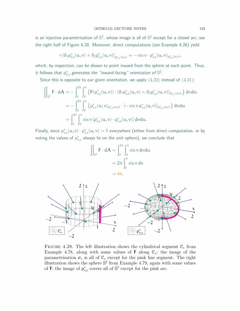
(MTH5113) LECTURE NOTES 133
is an injective parametrisation of S2, whose image is all of S2 except for a closed arc; seethe right half of Figure 4.28. Moreover, direct computations (see Example 4.26) yield
+[∂1ρ∗s,z(u, v)× ∂2ρ
∗s,z(u, v)]ρ∗s,z(u,v) = − sin v · ρ∗
s,z(u, v)ρ∗s,z(u,v),
which, by inspection, can be shown to point inward from the sphere at each point. Thus,it follows that ρ∗
s,z generates the “inward-facing” orientation of S2.Since this is opposite to our given orientation, we apply (4.22) instead of (4.21):∫∫
S2F · dA = −
∫ 2π
0
∫π
0
{F(ρ∗
s,z(u, v)) · [∂1ρ∗s,z(u, v)× ∂2ρ
∗s,z(u, v)]ρ∗s,z(u,v)
}dvdu
= −
∫ 2π
0
∫π
0
{ρ∗s,z(u, v)ρ∗s,z(u,v) · [− sin v ρ∗
s,z(u, v)]ρ∗s,z(u,v)}dvdu
=
∫ 2π
0
∫π
0
sin v [ρ∗s,z(u, v) · ρ∗
s,z(u, v)]dvdu.
Finally, since ρ∗s,z(u, v) · ρ∗
s,z(u, v) = 1 everywhere (either from direct computation, or bynoting the values of ρ∗
s,z always lie on the unit sphere), we conclude that∫∫S2F · dA =
∫ 2π
0
∫π
0
sin v dvdu
= 2π
∫π
0
sin v dv
= 4π.
−2−1
12
−2
2
1
2
x
y
z
C∗
−2−1
12
−2
2
−2
−1
1
2
x
y
z
ρ∗s,z
Figure 4.28. The left illustration shows the cylindrical segment C∗ fromExample 4.78, along with some values of F along C∗; the image of theparametrisation σ∗ is all of C∗ except for the pink line segment. The rightillustration shows the sphere S2 from Example 4.79, again with some valuesof F; the image of ρ∗
s,z covers all of S2 except for the pink arc.
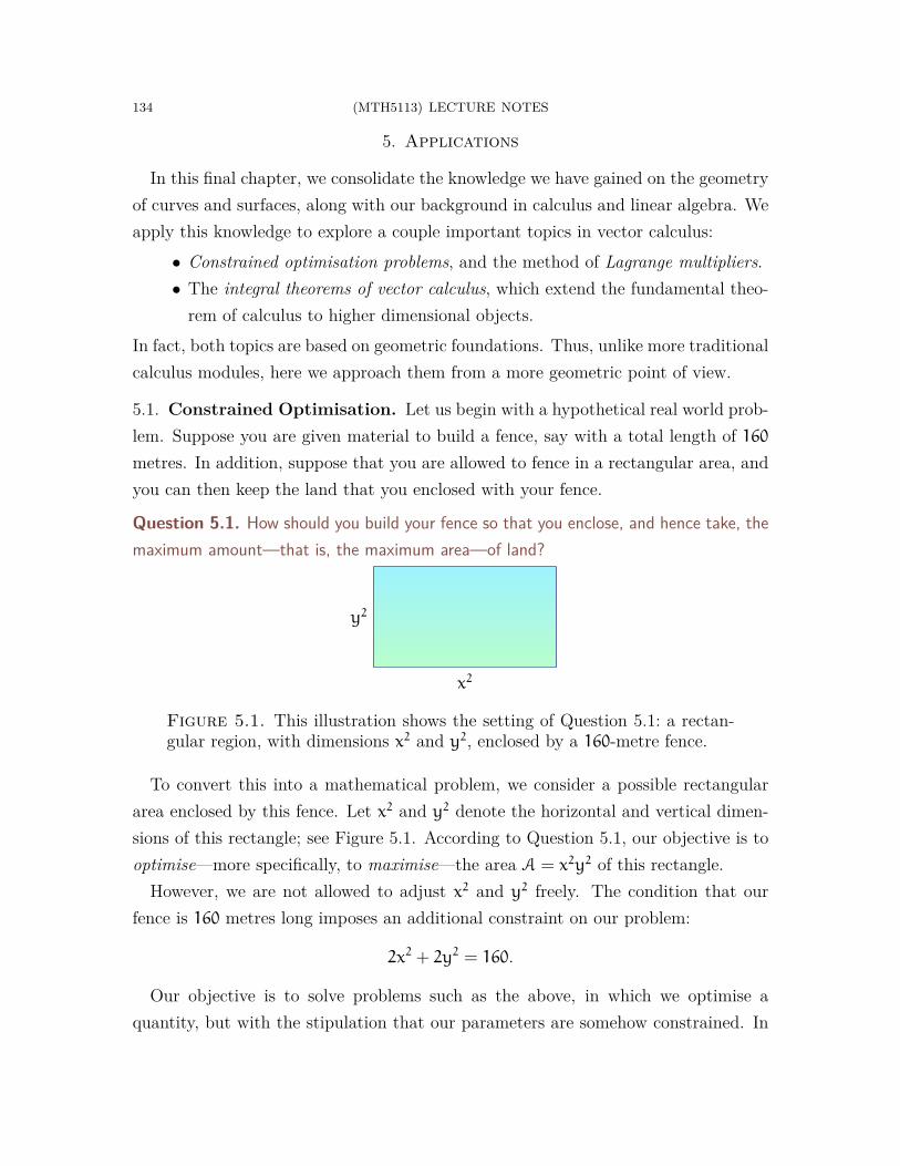
134 (MTH5113) LECTURE NOTES
5. Applications
In this final chapter, we consolidate the knowledge we have gained on the geometryof curves and surfaces, along with our background in calculus and linear algebra. Weapply this knowledge to explore a couple important topics in vector calculus:
• Constrained optimisation problems, and the method of Lagrange multipliers.• The integral theorems of vector calculus, which extend the fundamental theo-
rem of calculus to higher dimensional objects.In fact, both topics are based on geometric foundations. Thus, unlike more traditionalcalculus modules, here we approach them from a more geometric point of view.
5.1. Constrained Optimisation. Let us begin with a hypothetical real world prob-lem. Suppose you are given material to build a fence, say with a total length of 160metres. In addition, suppose that you are allowed to fence in a rectangular area, andyou can then keep the land that you enclosed with your fence.
Question 5.1. How should you build your fence so that you enclose, and hence take, themaximum amount—that is, the maximum area—of land?
x2
y2
Figure 5.1. This illustration shows the setting of Question 5.1: a rectan-gular region, with dimensions x2 and y2, enclosed by a 160-metre fence.
To convert this into a mathematical problem, we consider a possible rectangulararea enclosed by this fence. Let x2 and y2 denote the horizontal and vertical dimen-sions of this rectangle; see Figure 5.1. According to Question 5.1, our objective is tooptimise—more specifically, to maximise—the area A = x2y2 of this rectangle.
However, we are not allowed to adjust x2 and y2 freely. The condition that ourfence is 160 metres long imposes an additional constraint on our problem:
2x2 + 2y2 = 160.
Our objective is to solve problems such as the above, in which we optimise aquantity, but with the stipulation that our parameters are somehow constrained. In

(MTH5113) LECTURE NOTES 135
order to discuss the mathematics behind these problems, let us now widen our viewto more general classes of constrained optimisation problems:
Problem 5.2. Consider the following constrained optimisation problems:(1) Maximise or minimise f(x, y), subject to the constraint g(x, y) = c.(2) Maximise or minimise F(x, y, z), subject to the constraint G(x, y, z) = c.
The only difference between parts (1) and (2) in Problem 5.2 is the number ofvariables involved in both the constraint and the quantity to be optimised.
Let us first focus on Problem 5.2(1)—the two-variable case. Our first step towardunderstanding this problem, and toward developing a solution, is to connect it to thegeometric theory of curves that we have developed in earlier chapters.
Consider the set C of all points satisfying our constraint:
(5.1) C = {(x, y) ∈ R2 | g(x, y) = c}.
If g is “nice”, in that its gradient does not vanish anywhere on C, then Theorem 3.24implies that C is a curve. As a result, our constrained optimisation problem can beequivalently reformulated as a geometric optimisation problem:
Problem 5.3. Maximise or minimise f(p), for all points p on the curve C from (5.1).
Note this is similar to the problem of finding extrema (i.e. maxima or minima) offunctions that you studied in first-year calculus, except the functions are now definedon curves rather than on intervals. To attack this, we will combine our backgroundfrom first-year calculus with our knowledge on curve geometry.
The key idea behind Problem 5.3 is captured in the following theorem:
Theorem 5.4. Consider the curve (see Theorem 3.24)
C = {(x, y) ∈ U | g(x, y) = c},
where c ∈ R, where U ⊆ R2 is open and connected, and where g : U → R is a smoothfunction such that ∇g(q) is nonzero for every q ∈ C.
In addition, let f : U → R be another smooth function, and assume f achieves eitherits maximum or minimum value on C at a point p ∈ C. Then:
• ∇f(p) is normal to every element of TpC.• There exists λ ∈ R such that
(5.2) ∇f(p) = λ · ∇g(p).
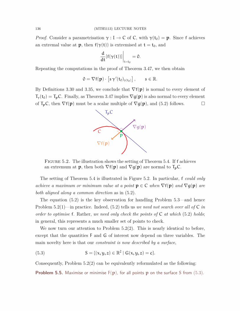
136 (MTH5113) LECTURE NOTES
Proof. Consider a parametrisation γ : I → C of C, with γ(t0) = p. Since f achievesan extremal value at p, then f(γ(t)) is extremised at t = t0, and
d
dt[f(γ(t))]
∣∣∣∣t=t0
= 0.
Repeating the computations in the proof of Theorem 3.47, we then obtain
0 = ∇f(p) ·[s γ ′(t0)γ(t0)
], s ∈ R.
By Definitions 3.30 and 3.35, we conclude that ∇f(p) is normal to every element ofTγ(t0) = TpC. Finally, as Theorem 3.47 implies ∇g(p) is also normal to every elementof TpC, then ∇f(p) must be a scalar multiple of ∇g(p), and (5.2) follows. □
C
TpC
p
∇f(p)
∇g(p)
Figure 5.2. The illustration shows the setting of Theorem 5.4. If f achievesan extremum at p, then both ∇f(p) and ∇g(p) are normal to TpC.
The setting of Theorem 5.4 is illustrated in Figure 5.2. In particular, f could onlyachieve a maximum or minimum value at a point p ∈ C when ∇f(p) and ∇g(p) areboth aligned along a common direction as in (5.2).
The equation (5.2) is the key observation for handling Problem 5.3—and henceProblem 5.2(1)—in practice. Indeed, (5.2) tells us we need not search over all of C inorder to optimise f. Rather, we need only check the points of C at which (5.2) holds;in general, this represents a much smaller set of points to check.
We now turn our attention to Problem 5.2(2). This is nearly identical to before,except that the quantities F and G of interest now depend on three variables. Themain novelty here is that our constraint is now described by a surface,
(5.3) S = {(x, y, z) ∈ R2 | G(x, y, z) = c}.
Consequently, Problem 5.2(2) can be equivalently reformulated as the following:
Problem 5.5. Maximise or minimise F(p), for all points p on the surface S from (5.3).

(MTH5113) LECTURE NOTES 137
To deal with Problem 5.5, we rely on the following geometric observations:
Theorem 5.6. Consider the surface (see Theorem 4.27)
S = {(x, y, z) ∈ U | G(x, y, z) = c},
where c ∈ R, where U ⊆ R3 is open and connected, and where G : U → R is a smoothfunction such that ∇G(q) is nonzero for every q ∈ S.
In addition, let F : U → R be another smooth function, and assume F achieves eitherits maximum or minimum value on S at a point p ∈ S. Then:
• ∇F(p) is normal to every element of TpS.• There exists λ ∈ R such that
(5.4) ∇F(p) = λ · ∇G(p).
Proof. Let σ : V → S be a parametrisation of S, with σ(u0, v0) = p. Then, we have
∂u[F(σ(u, v))]|(u,v)=(u0,v0) = 0, ∂v[F(σ(u, v))]|(u,v)=(u0,v0) = 0,
since F(σ(u, v)) is extremised when (u, v) = (u0, v0). Applying computations thatare analogous to the proof of Theorem 4.46 (in particular, the chain rule) yields
0 = ∇F(p) ·[a · ∂1σ(u0, v0)σ(u0,v0) + b · ∂2σ(u0, v0)σ(u0,v0)
], a, b ∈ R.
By Definitions 4.6 and 4.38, we see that ∇F(p) is normal to Tσ(u0, v0) = TpS. Finally,since both ∇F(p) and ∇G(p) are normal to TpS (see Theorem 4.46), it follows that∇F(p) must be a scalar multiple of ∇G(p), which is (5.4). □
∇G(p)
p
S
TpS ∇G(p)
∇F(p)
p
S
TpS
Figure 5.3. The illustrations show the setting of Theorem 5.6. In the leftplot, the gradient ∇G(p) (in purple) is normal to the tangent plane TpS.The right graphic shows the case in which F achieves an extremal value atp; here, both ∇F(p) and ∇G(p) are normal to TpS.

138 (MTH5113) LECTURE NOTES
The conclusions from Theorem 5.6 are analogous to those from Theorem 5.4. Inthe context of Problem 5.5, we see that we need not consider all of S when seeking tooptimise F. Indeed, we need only check the points of S at which (5.4) holds.
5.2. Lagrange Multipliers. We have discussed how Theorems 5.4 and 5.6 can con-tribute toward solving Problem 5.2, in particular by restricting the possible pointswhere extrema can occur. From this observation, we can now craft a process, knownas the method of Lagrange multipliers, for dealing with Problem 5.2.
Let us first look at constrained optimisation problems with two variables—Problem5.2(1). Here, the method of Lagrange multipliers can be summarised as follows:
• Step 1. Consider the following system of equations:
(5.5) ∂1f(x, y) = λ · ∂1g(x, y), ∂2f(x, y) = λ · ∂2g(x, y), g(x, y) = c.
• Step 2. Solve the system (5.5) for the unknowns x, y, λ ∈ R.• Step 3. For each solution (x, y, λ) from Step 2, check directly whether (x, y)
is a maximum or a minimum of f, subject to the constraint g(x, y) = c.Notice that the third equation in (5.5) is simply our given constraint. Furthermore,first two equations in (5.5) capture the gradient relation (5.2).
Remark 5.7. The term “Lagrange multiplier” refers to the real constant λ in (5.5), whichis an extra unknown that needs to be found. The method is named after Joseph-LouisLagrange (French and Italian mathematician, 1736–1813).
Example 5.8. To demonstrate how the method of Lagrange multipliers works, let usapply it to the original fence-building problem that was posed in Question 5.1: maximisethe quantity x2y2, subject to the constraint x2 + y2 = 80.
To set up the system (5.5), we define the functions
f(x, y) = x2y2, g(x, y) = x2 + y2, (x, y) ∈ R2,
representing the quantity to be optimised and the constraint, respectively. Note that
∂1f(x, y) = 2xy2, ∂2f(x, y) = 2x2y,
∂1g(x, y) = 2x, ∂2g(x, y) = 2y.
As a result, the system that we must solve is
(5.6) 2xy2 = λ · 2x, 2x2y = λ · 2y, x2 + y2 = 80.
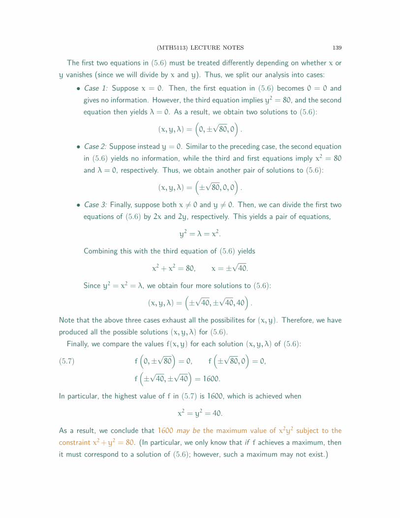
(MTH5113) LECTURE NOTES 139
The first two equations in (5.6) must be treated differently depending on whether x ory vanishes (since we will divide by x and y). Thus, we split our analysis into cases:
• Case 1: Suppose x = 0. Then, the first equation in (5.6) becomes 0 = 0 andgives no information. However, the third equation implies y2 = 80, and the secondequation then yields λ = 0. As a result, we obtain two solutions to (5.6):
(x, y, λ) =(0,±
√80, 0
).
• Case 2: Suppose instead y = 0. Similar to the preceding case, the second equationin (5.6) yields no information, while the third and first equations imply x2 = 80
and λ = 0, respectively. Thus, we obtain another pair of solutions to (5.6):
(x, y, λ) =(±√80, 0, 0
).
• Case 3: Finally, suppose both x 6= 0 and y 6= 0. Then, we can divide the first twoequations of (5.6) by 2x and 2y, respectively. This yields a pair of equations,
y2 = λ = x2.
Combining this with the third equation of (5.6) yields
x2 + x2 = 80, x = ±√40.
Since y2 = x2 = λ, we obtain four more solutions to (5.6):
(x, y, λ) =(±√40,±
√40, 40
).
Note that the above three cases exhaust all the possibilites for (x, y). Therefore, we haveproduced all the possible solutions (x, y, λ) for (5.6).
Finally, we compare the values f(x, y) for each solution (x, y, λ) of (5.6):
f(0,±
√80)= 0, f
(±√80, 0
)= 0,(5.7)
f(±√40,±
√40)= 1600.
In particular, the highest value of f in (5.7) is 1600, which is achieved when
x2 = y2 = 40.
As a result, we conclude that 1600 may be the maximum value of x2y2 subject to theconstraint x2+y2 = 80. (In particular, we only know that if f achieves a maximum, thenit must correspond to a solution of (5.6); however, such a maximum may not exist.)
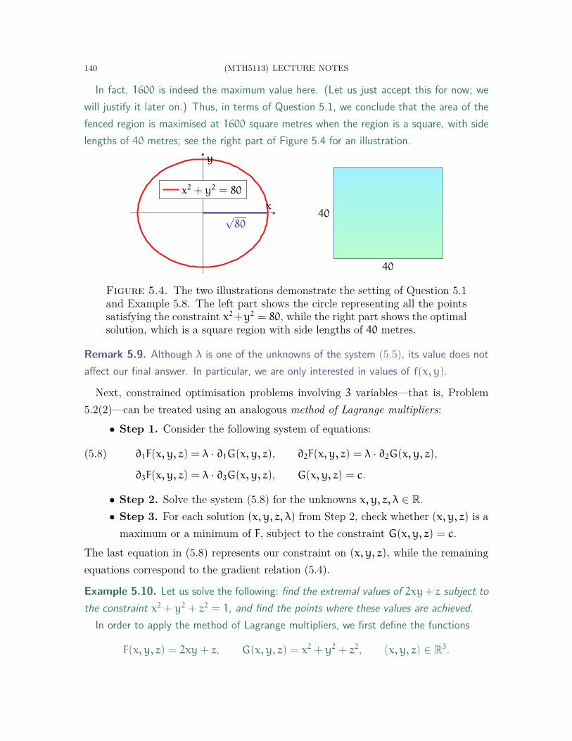
140 (MTH5113) LECTURE NOTES
In fact, 1600 is indeed the maximum value here. (Let us just accept this for now; wewill justify it later on.) Thus, in terms of Question 5.1, we conclude that the area of thefenced region is maximised at 1600 square metres when the region is a square, with sidelengths of 40 metres; see the right part of Figure 5.4 for an illustration.
√80
x
y
x2 + y2 = 80
40
40
Figure 5.4. The two illustrations demonstrate the setting of Question 5.1and Example 5.8. The left part shows the circle representing all the pointssatisfying the constraint x2+y2 = 80, while the right part shows the optimalsolution, which is a square region with side lengths of 40 metres.
Remark 5.9. Although λ is one of the unknowns of the system (5.5), its value does notaffect our final answer. In particular, we are only interested in values of f(x, y).
Next, constrained optimisation problems involving 3 variables—that is, Problem5.2(2)—can be treated using an analogous method of Lagrange multipliers:
• Step 1. Consider the following system of equations:
∂1F(x, y, z) = λ · ∂1G(x, y, z), ∂2F(x, y, z) = λ · ∂2G(x, y, z),(5.8)
∂3F(x, y, z) = λ · ∂3G(x, y, z), G(x, y, z) = c.
• Step 2. Solve the system (5.8) for the unknowns x, y, z, λ ∈ R.• Step 3. For each solution (x, y, z, λ) from Step 2, check whether (x, y, z) is a
maximum or a minimum of F, subject to the constraint G(x, y, z) = c.The last equation in (5.8) represents our constraint on (x, y, z), while the remainingequations correspond to the gradient relation (5.4).
Example 5.10. Let us solve the following: find the extremal values of 2xy+ z subject tothe constraint x2 + y2 + z2 = 1, and find the points where these values are achieved.
In order to apply the method of Lagrange multipliers, we first define the functions
F(x, y, z) = 2xy+ z, G(x, y, z) = x2 + y2 + z2, (x, y, z) ∈ R3.

(MTH5113) LECTURE NOTES 141
Observe that the partial derivatives of F and G satisfy
∂1F(x, y, z) = 2y, ∂2F(x, y, z) = 2x, ∂3F(x, y, z) = 1,
∂1G(x, y, z) = 2x, ∂2G(x, y, z) = 2y, ∂3G(x, y, z) = 2z.
Thus, the system (corresponding to (5.8)) that we must solve is
(5.9) 2y = 2λx, 2x = 2λy, 1 = 2λz, x2 + y2 + z2 = 1.
To solve (5.9) (which again involves dividing by x and y), we split into cases:
• Case 1: Suppose x = 0. Then, the first equation in (5.9) implies y = 0, and thefourth equation yields z2 = 1. Thus, in this case, we obtain the solutions
(x, y, z, λ) =
(0, 0,+1,+
1
2
), (x, y, z, λ) =
(0, 0,−1,−
1
2
)to (5.9). (Note the values of λ follow from the third equation in (5.9).) Further-more, the values of F corresponding to the above solutions are
(5.10) F(0, 0,±1) = ±1.
• Case 2: Suppose y = 0. The second equation of (5.9) then yields x = 0. Thus,we obtain the same solutions of (5.9) as in the preceding case.
• Case 3: Finally, suppose both x 6= 0 and y 6= 0. Then, dividing the first andsecond equations of (5.9) by 2x and 2y, respectively, we see that
y
x= λ =
x
y, x2 = y2.
From the above and the third equation of (5.9), we obtain two possibilities:
x = +y, λ = +1, z = +1
2,
x = −y, λ = −1, z = −1
2.
Combining the above with the constraint equation yields
x2 + x2 +
(±1
2
)2
= 1, x = ±√
3
8.
Thus, in this case, we end up with four solutions of (5.9):
(x1, y1, z1, λ1) =
(+
√3
8,+
√3
8,+
1
2,+1
), F(x1, y1, z1) = +
5
4,(5.11)
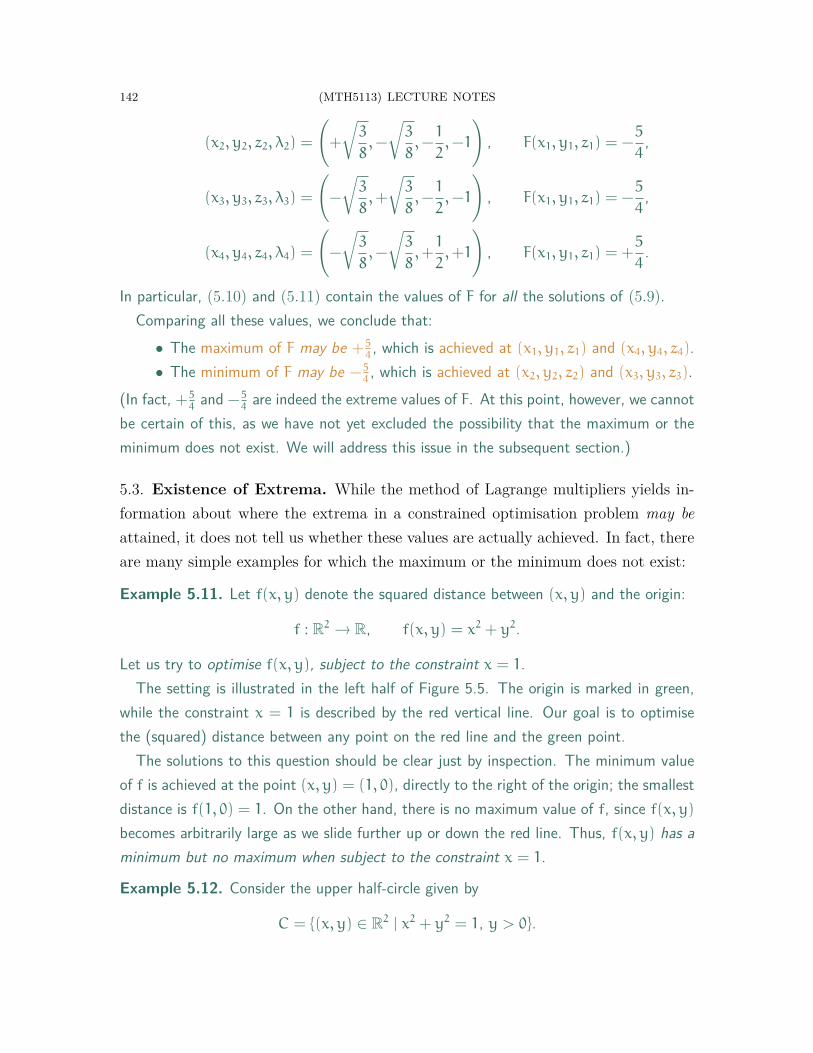
142 (MTH5113) LECTURE NOTES
(x2, y2, z2, λ2) =
(+
√3
8,−
√3
8,−
1
2,−1
), F(x1, y1, z1) = −
5
4,
(x3, y3, z3, λ3) =
(−
√3
8,+
√3
8,−
1
2,−1
), F(x1, y1, z1) = −
5
4,
(x4, y4, z4, λ4) =
(−
√3
8,−
√3
8,+
1
2,+1
), F(x1, y1, z1) = +
5
4.
In particular, (5.10) and (5.11) contain the values of F for all the solutions of (5.9).Comparing all these values, we conclude that:
• The maximum of F may be + 54, which is achieved at (x1, y1, z1) and (x4, y4, z4).
• The minimum of F may be − 54, which is achieved at (x2, y2, z2) and (x3, y3, z3).
(In fact, + 54
and − 54
are indeed the extreme values of F. At this point, however, we cannotbe certain of this, as we have not yet excluded the possibility that the maximum or theminimum does not exist. We will address this issue in the subsequent section.)
5.3. Existence of Extrema. While the method of Lagrange multipliers yields in-formation about where the extrema in a constrained optimisation problem may beattained, it does not tell us whether these values are actually achieved. In fact, thereare many simple examples for which the maximum or the minimum does not exist:
Example 5.11. Let f(x, y) denote the squared distance between (x, y) and the origin:
f : R2 → R, f(x, y) = x2 + y2.
Let us try to optimise f(x, y), subject to the constraint x = 1.The setting is illustrated in the left half of Figure 5.5. The origin is marked in green,
while the constraint x = 1 is described by the red vertical line. Our goal is to optimisethe (squared) distance between any point on the red line and the green point.
The solutions to this question should be clear just by inspection. The minimum valueof f is achieved at the point (x, y) = (1, 0), directly to the right of the origin; the smallestdistance is f(1, 0) = 1. On the other hand, there is no maximum value of f, since f(x, y)
becomes arbitrarily large as we slide further up or down the red line. Thus, f(x, y) has aminimum but no maximum when subject to the constraint x = 1.
Example 5.12. Consider the upper half-circle given by
C = {(x, y) ∈ R2 | x2 + y2 = 1, y > 0}.
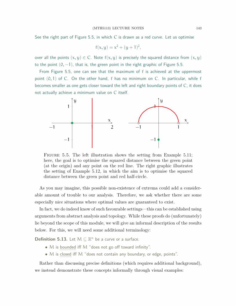
(MTH5113) LECTURE NOTES 143
See the right part of Figure 5.5, in which C is drawn as a red curve. Let us optimise
f(x, y) = x2 + (y+ 1)2,
over all the points (x, y) ∈ C. Note f(x, y) is precisely the squared distance from (x, y)
to the point (0,−1), that is, the green point in the right graphic of Figure 5.5.From Figure 5.5, one can see that the maximum of f is achieved at the uppermost
point (0, 1) of C. On the other hand, f has no minimum on C. In particular, while f
becomes smaller as one gets closer toward the left and right boundary points of C, it doesnot actually achieve a minimum value on C itself.
−1 1 2
−1
1
x
y
−1 1
−1
1
x
y
Figure 5.5. The left illustration shows the setting from Example 5.11;here, the goal is to optimise the squared distance between the green point(at the origin) and any point on the red line. The right graphic illustratesthe setting of Example 5.12, in which the aim is to optimise the squareddistance between the green point and red half-circle.
As you may imagine, this possible non-existence of extrema could add a consider-able amount of trouble to our analysis. Therefore, we ask whether there are someespecially nice situations where optimal values are guaranteed to exist.
In fact, we do indeed know of such favourable settings—this can be established usingarguments from abstract analysis and topology. While these proofs do (unfortunately)lie beyond the scope of this module, we will give an informal description of the resultsbelow. For this, we will need some additional terminology:
Definition 5.13. Let M ⊆ Rn be a curve or a surface.• M is bounded iff M “does not go off toward infinity”.• M is closed iff M “does not contain any boundary, or edge, points”.
Rather than discussing precise definitions (which requires additional background),we instead demonstrate these concepts informally through visual examples:
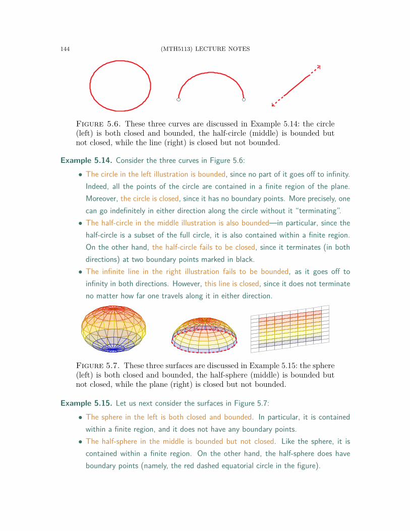
144 (MTH5113) LECTURE NOTES
Figure 5.6. These three curves are discussed in Example 5.14: the circle(left) is both closed and bounded, the half-circle (middle) is bounded butnot closed, while the line (right) is closed but not bounded.
Example 5.14. Consider the three curves in Figure 5.6:• The circle in the left illustration is bounded, since no part of it goes off to infinity.
Indeed, all the points of the circle are contained in a finite region of the plane.Moreover, the circle is closed, since it has no boundary points. More precisely, onecan go indefinitely in either direction along the circle without it “terminating”.
• The half-circle in the middle illustration is also bounded—in particular, since thehalf-circle is a subset of the full circle, it is also contained within a finite region.On the other hand, the half-circle fails to be closed, since it terminates (in bothdirections) at two boundary points marked in black.
• The infinite line in the right illustration fails to be bounded, as it goes off toinfinity in both directions. However, this line is closed, since it does not terminateno matter how far one travels along it in either direction.
Figure 5.7. These three surfaces are discussed in Example 5.15: the sphere(left) is both closed and bounded, the half-sphere (middle) is bounded butnot closed, while the plane (right) is closed but not bounded.
Example 5.15. Let us next consider the surfaces in Figure 5.7:• The sphere in the left is both closed and bounded. In particular, it is contained
within a finite region, and it does not have any boundary points.• The half-sphere in the middle is bounded but not closed. Like the sphere, it is
contained within a finite region. On the other hand, the half-sphere does haveboundary points (namely, the red dashed equatorial circle in the figure).
(MTH5113) LECTURE NOTES 145
• The infinite plane on the right is closed but not bounded. In particular, the planehas no boundary points at which it terminates, but it does go off to infinity.
Remark 5.16. Of course, there do exist precise, formal definitions of closed and boundedsets. These topics are further explored in MTH6127: Metric Spaces and Topology.
The main result regarding the existence of extrema is stated below:
Theorem 5.17. Let M ⊆ Rn be a curve or a surface, and let f be a smooth real-valuedfunction whose domain includes M. If M is both closed and bounded, then f achievesboth a maximum value and a minimum value on M.
Remark 5.18. Theorem 5.17 is a consequence of the Heine–Borel theorem from realanalysis. This is also further explored in MTH6127: Metric Spaces and Topology.
In particular, Examples 5.14 and 5.15 show that both circles and spheres are closedand bounded. Thus, it is convenient to consider problems with constraints givenby circles or spheres, since Theorem 5.17 guarantees that we must achieve both amaximum and a minimum. Moreover, by Theorems 5.4 and 5.6, we know that theseextrema can always be found through the method of Lagrange multipliers.
Example 5.19. We return to the problem, from Example 5.8, of finding the maximumof f(x, y) = x2y2 subject to the constraint x2 + y2 = 80. Note the constraint curve,
C = {(x, y) ∈ R2 | x2 + y2 = 80},
which is a circle of radius√80, is both closed and bounded; see the left graphic in Figure
5.4. Then, from Theorems 5.4 and 5.17, we deduce that the maximum of f exists, andthat it must be achieved at a point corresponding to a solution of the system (5.6).
To find this maximum of f, we need only compare all the values of f at the solutionpoints of (5.6). This was already done in (5.7), where we found that the largest valueof f is 1600. This proves that the maximum value of f(x, y), subject to the constraintx2 + y2 = 80, is 1600, and this maximum is achieved whenever x2 = y2 = 40.
Example 5.20. Returning to Example 5.10, we again notice that the constraint surface,
S = {(x, y, z) ∈ R3 | x2 + y2 + z2 = 1},
a unit sphere, is both closed and bounded. Theorem 5.17 then implies F(x, y, z) = 2xy+z
achieves both a maximum and a minimum value on S. To find these extrema, we againcompare the values of F at the solution points of (5.9).

146 (MTH5113) LECTURE NOTES
This was already done in (5.10) and (5.11); from there, we conclude that the maximumvalue of 2xy + z, subject to the constraint x2 + y2 + z2 = 1, is + 5
4, and this value is
achieved at the points (x1, y1, z1) and (x4, y4, z4). Similarly, the minimum value is − 54,
and this value is achieved at (x2, y2, z2) and (x3, y3, z3).
Finally, when a curve or surface M fails to be closed or bounded, the analysisbecomes more complicated. Here, one has several possibilities to consider:
(1) A maximum or minimum value is achieved at a point of M. The value and thepoint can then be found via the method of Lagrange multipliers, as before.
(2) One could approach a maximum or minimum at a boundary point of M.(3) One could also approach a maximum or minimum “toward infinity”.
If either case (2) or case (3) occurs, then a maximum or a minimum value does notexist, since neither the boundary of M nor “infinity” are points of M.
Example 5.21. As a simple example, let us optimise f(x, y) = y2 on the half-line
L = {(x, y) ∈ R2 | x = 0, y > −1}.
(The constraint is g(x, y) = x = 0, with the additional restriction y > −1.)To find potential extrema on L, we first apply the method of Lagrange multipliers.
Here, the system corresponding to (5.5), with the above f and g, is given by
0 = λ · 1, 2y = λ · 0, x = 0,
which only has one solution corresponding to a point of L:
(5.12) (x, y, λ) = (0, 0, 0), f(0, 0) = 0.
Since L has a boundary point (0,−1), we must also check what happens there. Here,we see that as one approaches (0,−1), the value of f approaches
(5.13) f(0,−1) = 1.
Also, since L is unbounded, we must also check what happens as one goes “towardinfinity” along L. Here, as one traverses infinitely far up L, the value of f approaches
(5.14) limy↗+∞ f(0, y) = +∞.
Finally, comparing the values of f in (5.12)–(5.14), we conclude that:• f attains a genuine minimum value, 0, at the point (0, 0) ∈ L.
(MTH5113) LECTURE NOTES 147
• f does not attain a maximum value on L. Instead, the largest value (+∞) of f isreached as one goes upward toward infinity along L.
On the other hand, the value of f at the boundary point (0,−1) of L (which, by definition,is not counted as a point of L) is not an extremum.
5.4. Conservative Fields. The final topics for this module involve integral theoremsfrom vector calculus, which, though usually associated with calculus, are geometricin nature. Let us first recall the familiar fundamental theorem of calculus:
(5.15)∫b
a
f ′(x)dx = f(b) − f(a).
While you should already know (5.15) intimately by now, here we note the following:• The left-hand side is an integral, over the 1-dimensional interval (a, b). More-
over, the integrand here is the derivative of a function f.• The right-hand side is the difference between the values of f at b and a. This
can be viewed as an integral of f over the 0-dimensional boundary of (a, b).The general question we want to pose is the following:
Question 5.22. Are there geometric generalisations of the fundamental theorem of cal-culus? Also, do these generalisations extend to higher dimensional settings?
First, let us see what happens when the interval (a, b) in (5.15) is replaced by anoriented curve. The general result is give by the following theorem:
Theorem 5.23. Let C ⊆ Rn be a bounded oriented curve, and suppose p,q ∈ Rn arethe initial and final points of C, respectively. Then, for any smooth map f : U → R, forwhich its domain U ⊆ Rn contains C, p, and q, we have the identity
(5.16)∫C
∇f · ds = f(q) − f(p).
Let us not be too precise on the definitions of initial and final points in Theorem5.23, though the intuition should be clear. Here, we simply informally view p and q
as the endpoints of C, arranged so that C goes from p to q; see Figure 5.8.
Proof of Theorem 5.23. The assumptions imposed on C—as well as on p and q—imply there exists an injective parametrisation γ : (a, b) → C of C satisfying
limt↘a
γ(t) = p, limt↗b
γ(t) = q.
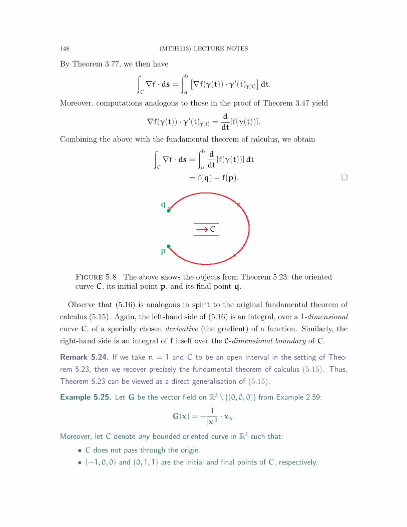
148 (MTH5113) LECTURE NOTES
By Theorem 3.77, we then have∫C
∇f · ds =
∫b
a
[∇f(γ(t)) · γ ′(t)γ(t)
]dt.
Moreover, computations analogous to those in the proof of Theorem 3.47 yield
∇f(γ(t)) · γ ′(t)γ(t) =d
dt[f(γ(t))].
Combining the above with the fundamental theorem of calculus, we obtain∫C
∇f · ds =
∫b
a
d
dt[f(γ(t))]dt
= f(q) − f(p). □
p
q
C
Figure 5.8. The above shows the objects from Theorem 5.23: the orientedcurve C, its initial point p, and its final point q.
Observe that (5.16) is analogous in spirit to the original fundamental theorem ofcalculus (5.15). Again, the left-hand side of (5.16) is an integral, over a 1-dimensionalcurve C, of a specially chosen derivative (the gradient) of a function. Similarly, theright-hand side is an integral of f itself over the 0-dimensional boundary of C.
Remark 5.24. If we take n = 1 and C to be an open interval in the setting of Theo-rem 5.23, then we recover precisely the fundamental theorem of calculus (5.15). Thus,Theorem 5.23 can be viewed as a direct generalisation of (5.15).
Example 5.25. Let G be the vector field on R3 \ {(0, 0, 0)} from Example 2.59:
G(x) = −1
|x|3· x x.
Moreover, let C denote any bounded oriented curve in R3 such that:• C does not pass through the origin.• (−1, 0, 0) and (0, 1, 1) are the initial and final points of C, respectively.

(MTH5113) LECTURE NOTES 149
Let us now integrate G over this curve C.The key observation comes from Example 2.65, namely, that G can be expressed as a
gradient, G = ∇g, where g is the real-valued function
g : R3 \ {(0, 0, 0)} → R, g(p) =1
|p|.
By our assumptions for C, we see that g is well-defined on both C and its endpoints. Asa result, applying Theorem 5.23 to C and g, we conclude that∫
C
G · ds =
∫C
∇g · ds
= g(0, 1, 1) − g(−1, 0, 0)
=1√2− 1.
Recall also, from Example 2.59, that G represents the Newtonian gravitational forceexerted by a particle at the origin. As a result, the integral of G over C represents the totalwork done by this gravitational force on another object travelling along C, from (−1, 0, 0)
to (0, 1, 1). In particular, observe that the work done depends only on the values of thegravitational potential g at the endpoints of C.
qp
Figure 5.9. The above illustration shows oriented curves starting and end-ing at common points p and q, respectively. Integrating a gradient ∇f alongany of these oriented curves will yield the same value.
Example 5.25 illuminates a rather interesting consequence of Theorem 5.23. Re-turning to the abstract setting of the theorem, suppose wish to compute∫
C
∇f · ds.
Then, (5.16) implies that, although the above integral involves the values of f on allof C, it ultimately depends only on the values of f at the endpoints p and q.

150 (MTH5113) LECTURE NOTES
In addition, consider a different bounded oriented curve, C ′, which has the sameinitial and final points as C. Then, applying Theorem 5.23 twice, we see that∫
C ′∇f · ds = f(q) − f(p)
=
∫C
∇f · ds.
In particular, even though C and C ′ may be radically different, Theorem 5.23 ensuresthat the integrals of ∇f over C and C ′ must be the same. Moreover, this holds for anypair of curves, provided they have the same starting and end points; see Figure 5.9.
In summary, we conclude that curve integrals of ∇f are independent of path, in thatthe values of these integrals do not depend on what the designated curve is doing, butonly on where the curve begins and ends. In other words, we can think of gradientsas belonging to a very special class of vector fields.
Definition 5.26. Let F be a vector field on an open and connected subset U ⊆ Rn.We say that F is conservative iff for any p,q ∈ U, and for any bounded oriented curvesC,C ′ ⊆ U with both the same initial point p and the same final point q, we have
(5.17)∫C
F · ds =
∫C ′F · ds.
While Theorem 5.23 implies that gradients are conservative fields, the converse isalso true: every conservative field is the gradient of some real-valued function.
Theorem 5.27. Let F be a smooth vector field on an open and connected subset U ⊆ Rn.Then, F is conservative if and only if there is a smooth f : U → R such that F = ∇f.
Proof. See the MTH5102: Calculus III lecture notes [2] or a calculus textbook (e.g.[10]) for details. In fact, if F is conservative, then for a fixed p0 ∈ U, one can define
f(p) =
∫C(p)
F · ds, p ∈ U,
where C(p) ⊆ U is any oriented curve with starting point p0 and final point p. □
Remark 5.28. The term “conservative fields” comes from physics, as such vector fieldsrepresent forces within systems that have a conserved energy.
5.5. Green’s Theorem. The next step is to take the viewpoint we have developedwith the fundamental theorem of calculus (5.15) and its generalisation, Theorem 5.23,and to then explore their analogues in higher dimensions.
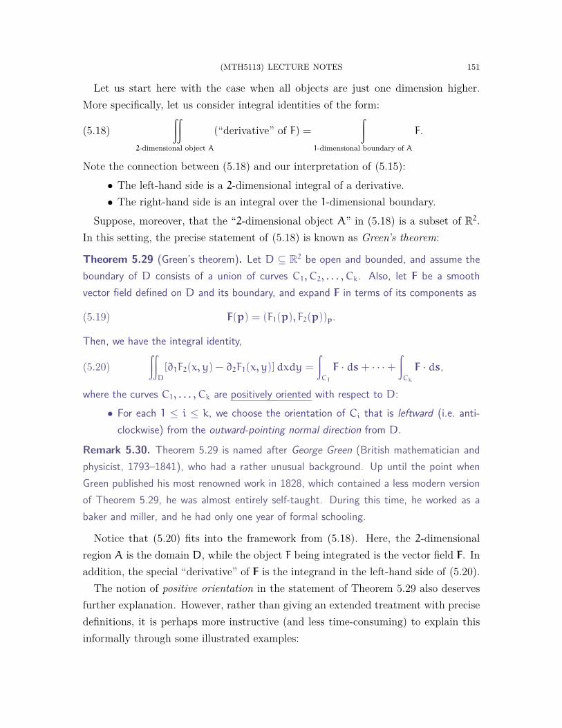
(MTH5113) LECTURE NOTES 151
Let us start here with the case when all objects are just one dimension higher.More specifically, let us consider integral identities of the form:
(5.18)∫∫
2-dimensional object A
(“derivative” of F) =∫
1-dimensional boundary of A
F.
Note the connection between (5.18) and our interpretation of (5.15):• The left-hand side is a 2-dimensional integral of a derivative.• The right-hand side is an integral over the 1-dimensional boundary.
Suppose, moreover, that the “2-dimensional object A” in (5.18) is a subset of R2.In this setting, the precise statement of (5.18) is known as Green’s theorem:
Theorem 5.29 (Green’s theorem). Let D ⊆ R2 be open and bounded, and assume theboundary of D consists of a union of curves C1, C2, . . . , Ck. Also, let F be a smoothvector field defined on D and its boundary, and expand F in terms of its components as
(5.19) F(p) = (F1(p), F2(p))p.
Then, we have the integral identity,
(5.20)∫∫
D
[∂1F2(x, y) − ∂2F1(x, y)]dxdy =
∫C1
F · ds+ · · ·+∫Ck
F · ds,
where the curves C1, . . . , Ck are positively oriented with respect to D:• For each 1 ≤ i ≤ k, we choose the orientation of Ci that is leftward (i.e. anti-
clockwise) from the outward-pointing normal direction from D.
Remark 5.30. Theorem 5.29 is named after George Green (British mathematician andphysicist, 1793–1841), who had a rather unusual background. Up until the point whenGreen published his most renowned work in 1828, which contained a less modern versionof Theorem 5.29, he was almost entirely self-taught. During this time, he worked as abaker and miller, and he had only one year of formal schooling.
Notice that (5.20) fits into the framework from (5.18). Here, the 2-dimensionalregion A is the domain D, while the object F being integrated is the vector field F. Inaddition, the special “derivative” of F is the integrand in the left-hand side of (5.20).
The notion of positive orientation in the statement of Theorem 5.29 also deservesfurther explanation. However, rather than giving an extended treatment with precisedefinitions, it is perhaps more instructive (and less time-consuming) to explain thisinformally through some illustrated examples:
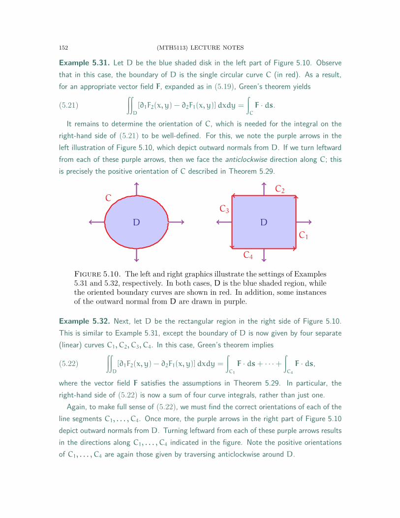
152 (MTH5113) LECTURE NOTES
Example 5.31. Let D be the blue shaded disk in the left part of Figure 5.10. Observethat in this case, the boundary of D is the single circular curve C (in red). As a result,for an appropriate vector field F, expanded as in (5.19), Green’s theorem yields
(5.21)∫∫
D
[∂1F2(x, y) − ∂2F1(x, y)]dxdy =
∫C
F · ds.
It remains to determine the orientation of C, which is needed for the integral on theright-hand side of (5.21) to be well-defined. For this, we note the purple arrows in theleft illustration of Figure 5.10, which depict outward normals from D. If we turn leftwardfrom each of these purple arrows, then we face the anticlockwise direction along C; thisis precisely the positive orientation of C described in Theorem 5.29.
D
C
D
C1
C2
C3
C4
Figure 5.10. The left and right graphics illustrate the settings of Examples5.31 and 5.32, respectively. In both cases, D is the blue shaded region, whilethe oriented boundary curves are shown in red. In addition, some instancesof the outward normal from D are drawn in purple.
Example 5.32. Next, let D be the rectangular region in the right side of Figure 5.10.This is similar to Example 5.31, except the boundary of D is now given by four separate(linear) curves C1, C2, C3, C4. In this case, Green’s theorem implies
(5.22)∫∫
D
[∂1F2(x, y) − ∂2F1(x, y)]dxdy =
∫C1
F · ds+ · · ·+∫C4
F · ds,
where the vector field F satisfies the assumptions in Theorem 5.29. In particular, theright-hand side of (5.22) is now a sum of four curve integrals, rather than just one.
Again, to make full sense of (5.22), we must find the correct orientations of each of theline segments C1, . . . , C4. Once more, the purple arrows in the right part of Figure 5.10depict outward normals from D. Turning leftward from each of these purple arrows resultsin the directions along C1, . . . , C4 indicated in the figure. Note the positive orientationsof C1, . . . , C4 are again those given by traversing anticlockwise around D.
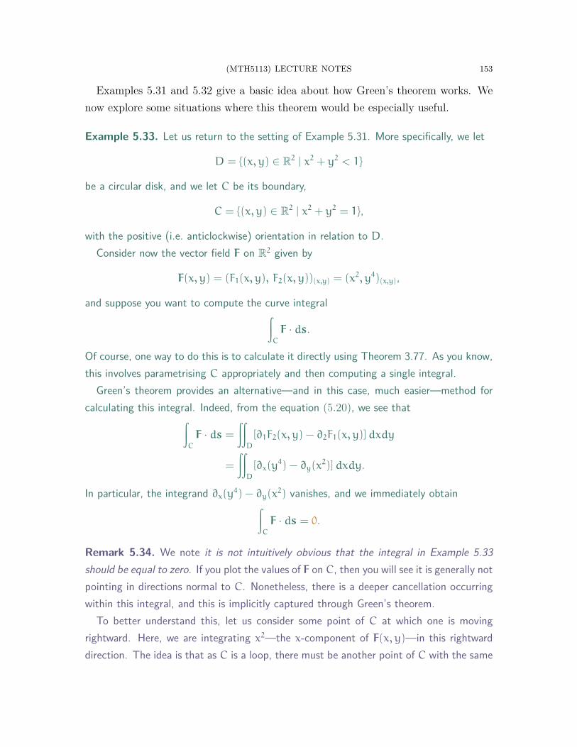
(MTH5113) LECTURE NOTES 153
Examples 5.31 and 5.32 give a basic idea about how Green’s theorem works. Wenow explore some situations where this theorem would be especially useful.
Example 5.33. Let us return to the setting of Example 5.31. More specifically, we let
D = {(x, y) ∈ R2 | x2 + y2 < 1}
be a circular disk, and we let C be its boundary,
C = {(x, y) ∈ R2 | x2 + y2 = 1},
with the positive (i.e. anticlockwise) orientation in relation to D.Consider now the vector field F on R2 given by
F(x, y) = (F1(x, y), F2(x, y))(x,y) = (x2, y4)(x,y),
and suppose you want to compute the curve integral∫C
F · ds.
Of course, one way to do this is to calculate it directly using Theorem 3.77. As you know,this involves parametrising C appropriately and then computing a single integral.
Green’s theorem provides an alternative—and in this case, much easier—method forcalculating this integral. Indeed, from the equation (5.20), we see that∫
C
F · ds =
∫∫D
[∂1F2(x, y) − ∂2F1(x, y)]dxdy
=
∫∫D
[∂x(y4) − ∂y(x
2)]dxdy.
In particular, the integrand ∂x(y4) − ∂y(x
2) vanishes, and we immediately obtain∫C
F · ds = 0.
Remark 5.34. We note it is not intuitively obvious that the integral in Example 5.33should be equal to zero. If you plot the values of F on C, then you will see it is generally notpointing in directions normal to C. Nonetheless, there is a deeper cancellation occurringwithin this integral, and this is implicitly captured through Green’s theorem.
To better understand this, let us consider some point of C at which one is movingrightward. Here, we are integrating x2—the x-component of F(x, y)—in this rightwarddirection. The idea is that as C is a loop, there must be another point of C with the same
154 (MTH5113) LECTURE NOTES
x-coordinate at which one is going leftward. Here, this leftward integral of x2 will cancelwith the previous rightward integral of x2. More generally, each point where we integratex2 rightward is cancelled by some corresponding point in which we integrate x2 leftward.
A similar argument can be made for vertical motion along C, with the y-componenty4 of F(x, y). As a result, the total integral of F over C must be 0.
For our next application, let us consider the region D ⊆ R2 drawn in Figure 5.11.Imagine that D represents the surface of a lake, and suppose you wish to find itsarea. Normally, to do this, you would probably take a boat out into the lake andmake various measurements as you sail about.
Now, suppose D is also full of ravenous giant sharks that have eaten your boat, soyou can no longer venture out onto the lake! Would you still be able to somehow findthe area of the lake, even though you are landbound?
In more abstract terms, the above question can be formulated as follows:
Question 5.35. Can we measure the area of a region D ⊆ R2 (say, the one from Figure5.11) using only information gathered at the boundary of D?
DC
Figure 5.11. Corollary 5.36 gives a way to compute the area of the (blue)region D using only the information on its (red) boundary curve C.
The key idea here is to look at the vector field A on R2, given by
(5.23) A(x, y) =1
2· (−y, x)(x,y).
In particular, if we were to apply Green’s theorem, with this vector field F = A andwith the region D in Figure 5.11, then a direct computation yields∫
C
A · ds =
∫∫D
[∂x
(1
2x
)− ∂y
(−1
2y
)]dxdy
=
∫∫D
1 dxdy.
(MTH5113) LECTURE NOTES 155
The above tells us that the area of D can be expressed in terms of an integral alongits boundary curve C. In other words, we need not venture into the lake D in order tomeasure its area! We need only go one lap around the edge C of the lake and sum upthe information read from A while doing so. (Observe that A contains informationabout one’s horizontal and vertical positions as one travels around the lake.)
Repeating the above for more general regions, we obtain the following result:
Corollary 5.36. Let D and C1, C2, . . . , Ck be as in the statement of Theorem 5.29.Moreover, let A be the vector field on R2 given by (5.23). Then,
(5.24) A(D) =
∫C1
A · ds+ · · ·+∫Ck
A · ds.
Remark 5.37. We mention that A is not the only vector field we can use here. Forexample, if we define another pair of vector fields Ax and Ay on R2 via the formulas
Ax(x, y) = (0, x)(x,y), Ay(x, y) = (−y, 0)(x,y),
then one can see that Corollary 5.36 still holds when A is replaced by either Ax or Ay.Remark 5.38. Unfortunately, we lack the time in this module to discuss the proof ofGreen’s theorem. However, let us mention that Green’s theorem can be derived as aspecial case of the divergence theorem, which we will discuss later on.
5.6. Divergence and Curl. We now take a brief detour from our study of integraltheorems to define two additional differential operations on vector fields: the diver-gence and curl. As we will soon see, these operations represent very special derivativesand will play prominent roles in upcoming integral theorems.
First, we look at the divergence, which maps vector fields to scalar functions:
Definition 5.39. Let U ⊆ Rn be open and connected. In addition, let F be a smoothvector field on U, and write F in terms of its components as
(5.25) F(p) = (F1(p), F2(p), . . . , Fn(p))p, p ∈ U.
We define the divergence of F, denoted ∇ · F or div F, to be the (real-valued) function
(5.26) (∇ · F) : U → R, (∇ · F)(p) = ∂1F1(p) + ∂2F2(p) + · · ·+ ∂nFn(p).
Remark 5.40. A helpful way to remember (5.26) is to write it as a “dot product”,
∇ · F = (∂1, ∂2, . . . , ∂n) · (F1, F2, . . . , Fn).

156 (MTH5113) LECTURE NOTES
The above is also the inspiration for the notation “∇ · F”.
Observe that although F(p) is an arrow starting at p, the corresponding divergence(∇·F)(p) is a scalar. Thus, do make sure that you are always dealing with the correcttype of object in your computations, so that you avoid getting confused!
Example 5.41. Consider the vector field F on R2 given by
F(x, y) = (F1(x, y), F2(x, y))(x,y) = (x, y)(x,y).
See the left illustration in Figure 5.12 for a partial plot of F.To find the divergence of F, we simply apply Definition 5.39 to each (x, y) ∈ R2:
(∇ · F)(x, y) = ∂1F1(x, y) + ∂2F2(x, y)
= ∂x(x) + ∂y(y)
= 2.
Thus, ∇ · F is a constant function, and the divergence of F at every point is 2.
−1 −0.5 0.5 1
−1
−0.5
0.5
1
x
y
−2 2
−2
2
x
y
Figure 5.12. The arrows in the left plot represent several values of thevector field F from Example 5.41; similarly, the arrows in the right plotindicate some values of H from Example 5.42.
Example 5.42. Next, let H be the vector field on R2 given by
H(x, y) = (−y, x)(x,y).
(See the right plot in Figure 5.12.) Again, we can compute ∇ ·H using Definition 5.39:
(∇ ·H)(x, y) = ∂x(−y) + ∂y(x)
= 0.
In particular, ∇ ·H vanishes everywhere, i.e. H is divergence-free.
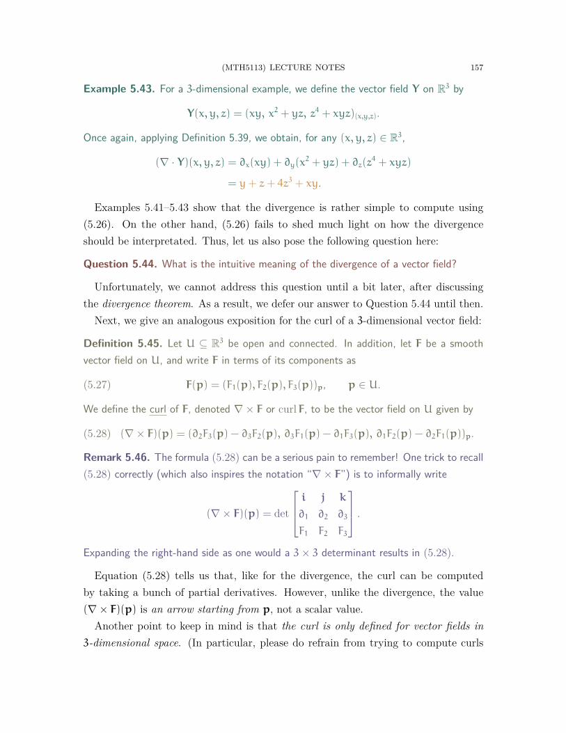
(MTH5113) LECTURE NOTES 157
Example 5.43. For a 3-dimensional example, we define the vector field Y on R3 by
Y(x, y, z) = (xy, x2 + yz, z4 + xyz)(x,y,z).
Once again, applying Definition 5.39, we obtain, for any (x, y, z) ∈ R3,
(∇ · Y)(x, y, z) = ∂x(xy) + ∂y(x2 + yz) + ∂z(z
4 + xyz)
= y+ z+ 4z3 + xy.
Examples 5.41–5.43 show that the divergence is rather simple to compute using(5.26). On the other hand, (5.26) fails to shed much light on how the divergenceshould be interpretated. Thus, let us also pose the following question here:
Question 5.44. What is the intuitive meaning of the divergence of a vector field?
Unfortunately, we cannot address this question until a bit later, after discussingthe divergence theorem. As a result, we defer our answer to Question 5.44 until then.
Next, we give an analogous exposition for the curl of a 3-dimensional vector field:
Definition 5.45. Let U ⊆ R3 be open and connected. In addition, let F be a smoothvector field on U, and write F in terms of its components as
(5.27) F(p) = (F1(p), F2(p), F3(p))p, p ∈ U.
We define the curl of F, denoted ∇× F or curl F, to be the vector field on U given by
(5.28) (∇× F)(p) = (∂2F3(p) − ∂3F2(p), ∂3F1(p) − ∂1F3(p), ∂1F2(p) − ∂2F1(p))p.
Remark 5.46. The formula (5.28) can be a serious pain to remember! One trick to recall(5.28) correctly (which also inspires the notation “∇× F”) is to informally write
(∇× F)(p) = det
i j k
∂1 ∂2 ∂3
F1 F2 F3
.
Expanding the right-hand side as one would a 3× 3 determinant results in (5.28).
Equation (5.28) tells us that, like for the divergence, the curl can be computedby taking a bunch of partial derivatives. However, unlike the divergence, the value(∇× F)(p) is an arrow starting from p, not a scalar value.
Another point to keep in mind is that the curl is only defined for vector fields in3-dimensional space. (In particular, please do refrain from trying to compute curls

158 (MTH5113) LECTURE NOTES
of 2-dimensional vector fields.) This again differs from the divergence, which is well-defined through (5.26) for vector fields in any dimension.
Example 5.47. Let X be the vector field on R3 defined by
X(x, y, z) = (X1(x, y, z), X2(x, y, z), X3(x, y, z))(x,y,z)
= (yz, xz, xy)(x,y,z).
Let us now find the curl of X.According to Definition 5.45, the components of ∇× X are given by
∂2X3(x, y, z) − ∂3X2(x, y, z) = ∂y(xy) − ∂z(xz)
= x− x
= 0,
∂3X1(x, y, z) − ∂1X3(x, y, z) = ∂z(yz) − ∂x(xy)
= y− y
= 0,
∂1X2(x, y, z) − ∂2X1(x, y, z) = ∂x(xz) − ∂y(yz)
= z− z
= 0.
As a result, by (5.28), we conclude that X is curl-free:
(∇× X)(x, y, z) = (0, 0, 0)(x,y,z), (x, y, z) ∈ R3.
Example 5.48. Let us return to the vector field Y from Example 5.43:
Y(x, y, z) = (Y1(x, y, z), Y2(x, y, z), Y3(x, y, z))(x,y,z)
= (xy, x2 + yz, z4 + xyz)(x,y,z).
By Definition 5.45, the components of ∇× Y satisfy
∂2Y3(x, y, z) − ∂3Y2(x, y, z) = ∂y(z4 + xyz) − ∂z(x
2 + yz)
= xz− y,
∂3Y1(x, y, z) − ∂1Y3(x, y, z) = ∂z(xy) − ∂x(z4 + xyz)
= −yz,
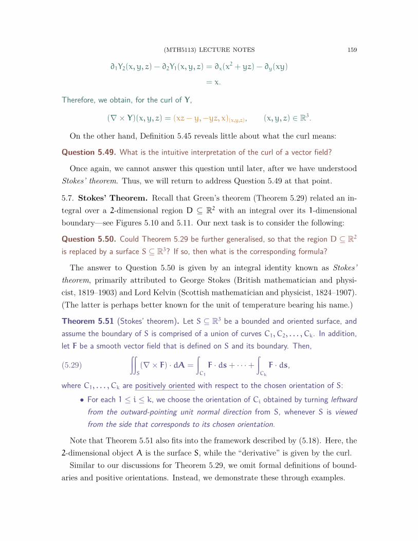
(MTH5113) LECTURE NOTES 159
∂1Y2(x, y, z) − ∂2Y1(x, y, z) = ∂x(x2 + yz) − ∂y(xy)
= x.
Therefore, we obtain, for the curl of Y ,
(∇× Y)(x, y, z) = (xz− y,−yz, x)(x,y,z), (x, y, z) ∈ R3.
On the other hand, Definition 5.45 reveals little about what the curl means:
Question 5.49. What is the intuitive interpretation of the curl of a vector field?
Once again, we cannot answer this question until later, after we have understoodStokes’ theorem. Thus, we will return to address Question 5.49 at that point.
5.7. Stokes’ Theorem. Recall that Green’s theorem (Theorem 5.29) related an in-tegral over a 2-dimensional region D ⊆ R2 with an integral over its 1-dimensionalboundary—see Figures 5.10 and 5.11. Our next task is to consider the following:
Question 5.50. Could Theorem 5.29 be further generalised, so that the region D ⊆ R2
is replaced by a surface S ⊆ R3? If so, then what is the corresponding formula?
The answer to Question 5.50 is given by an integral identity known as Stokes’theorem, primarily attributed to George Stokes (British mathematician and physi-cist, 1819–1903) and Lord Kelvin (Scottish mathematician and physicist, 1824–1907).(The latter is perhaps better known for the unit of temperature bearing his name.)
Theorem 5.51 (Stokes’ theorem). Let S ⊆ R3 be a bounded and oriented surface, andassume the boundary of S is comprised of a union of curves C1, C2, . . . , Ck. In addition,let F be a smooth vector field that is defined on S and its boundary. Then,
(5.29)∫∫
S
(∇× F) · dA =
∫C1
F · ds+ · · ·+∫Ck
F · ds,
where C1, . . . , Ck are positively oriented with respect to the chosen orientation of S:• For each 1 ≤ i ≤ k, we choose the orientation of Ci obtained by turning leftward
from the outward-pointing unit normal direction from S, whenever S is viewedfrom the side that corresponds to its chosen orientation.
Note that Theorem 5.51 also fits into the framework described by (5.18). Here, the2-dimensional object A is the surface S, while the “derivative” is given by the curl.
Similar to our discussions for Theorem 5.29, we omit formal definitions of bound-aries and positive orientations. Instead, we demonstrate these through examples.
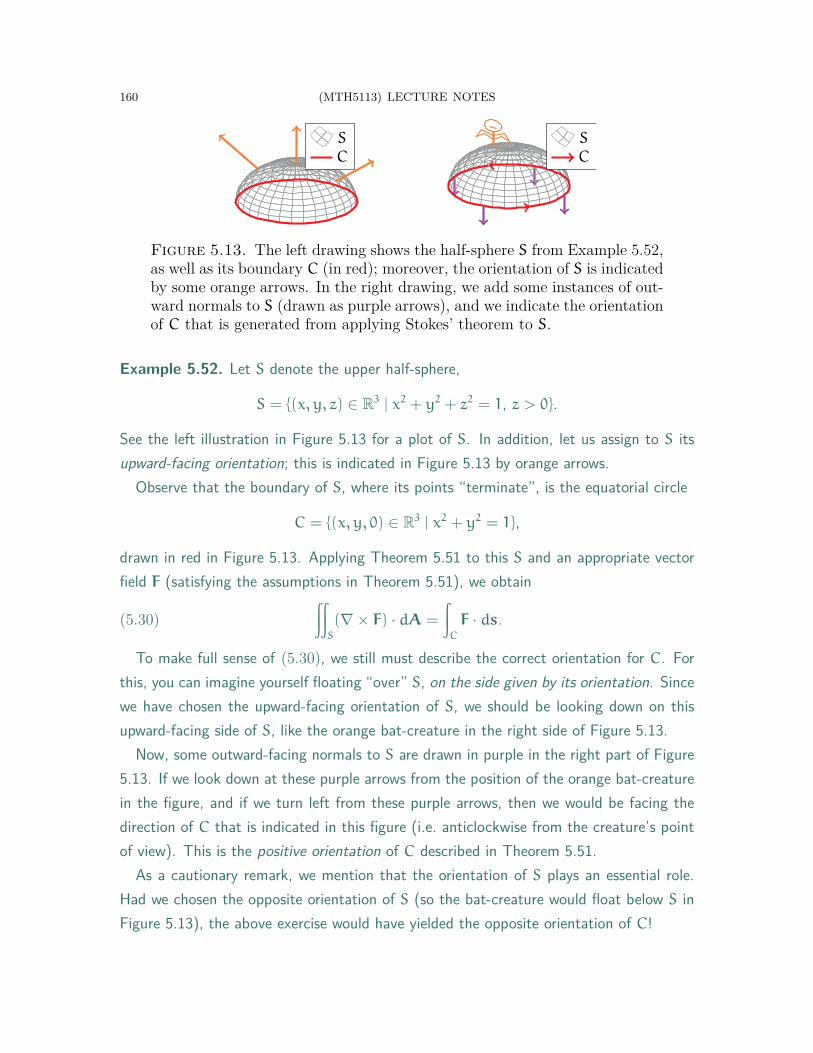
160 (MTH5113) LECTURE NOTES
S
C
S
C
Figure 5.13. The left drawing shows the half-sphere S from Example 5.52,as well as its boundary C (in red); moreover, the orientation of S is indicatedby some orange arrows. In the right drawing, we add some instances of out-ward normals to S (drawn as purple arrows), and we indicate the orientationof C that is generated from applying Stokes’ theorem to S.
Example 5.52. Let S denote the upper half-sphere,
S = {(x, y, z) ∈ R3 | x2 + y2 + z2 = 1, z > 0}.
See the left illustration in Figure 5.13 for a plot of S. In addition, let us assign to S itsupward-facing orientation; this is indicated in Figure 5.13 by orange arrows.
Observe that the boundary of S, where its points “terminate”, is the equatorial circle
C = {(x, y, 0) ∈ R3 | x2 + y2 = 1},
drawn in red in Figure 5.13. Applying Theorem 5.51 to this S and an appropriate vectorfield F (satisfying the assumptions in Theorem 5.51), we obtain
(5.30)∫∫
S
(∇× F) · dA =
∫C
F · ds.
To make full sense of (5.30), we still must describe the correct orientation for C. Forthis, you can imagine yourself floating “over” S, on the side given by its orientation. Sincewe have chosen the upward-facing orientation of S, we should be looking down on thisupward-facing side of S, like the orange bat-creature in the right side of Figure 5.13.
Now, some outward-facing normals to S are drawn in purple in the right part of Figure5.13. If we look down at these purple arrows from the position of the orange bat-creaturein the figure, and if we turn left from these purple arrows, then we would be facing thedirection of C that is indicated in this figure (i.e. anticlockwise from the creature’s pointof view). This is the positive orientation of C described in Theorem 5.51.
As a cautionary remark, we mention that the orientation of S plays an essential role.Had we chosen the opposite orientation of S (so the bat-creature would float below S inFigure 5.13), the above exercise would have yielded the opposite orientation of C!
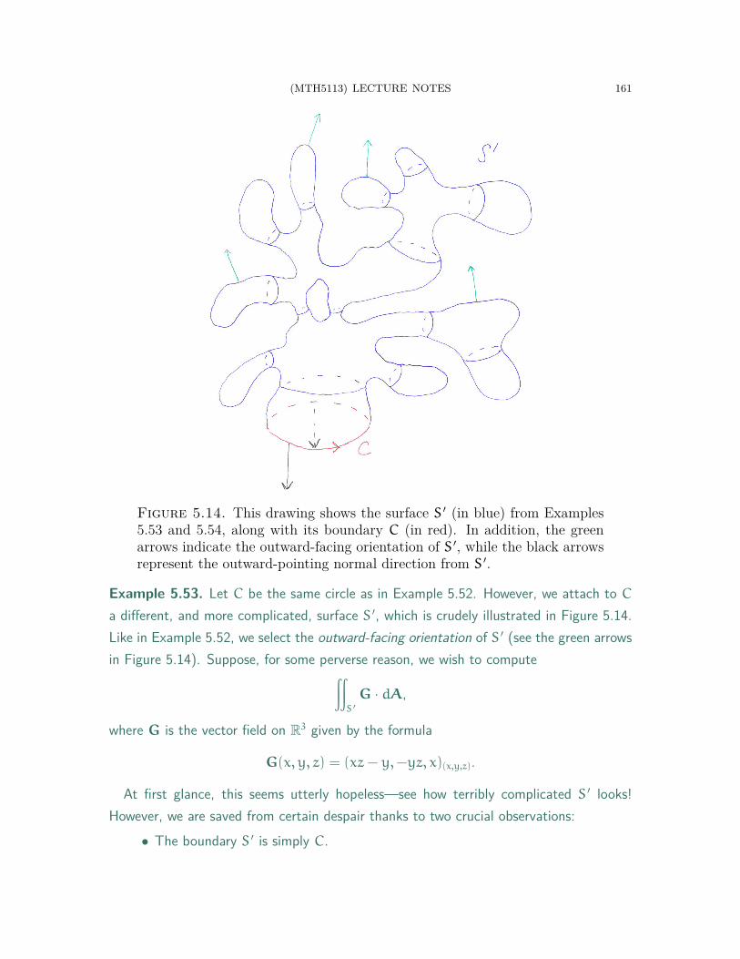
(MTH5113) LECTURE NOTES 161
Figure 5.14. This drawing shows the surface S ′ (in blue) from Examples5.53 and 5.54, along with its boundary C (in red). In addition, the greenarrows indicate the outward-facing orientation of S ′, while the black arrowsrepresent the outward-pointing normal direction from S ′.
Example 5.53. Let C be the same circle as in Example 5.52. However, we attach to C
a different, and more complicated, surface S ′, which is crudely illustrated in Figure 5.14.Like in Example 5.52, we select the outward-facing orientation of S ′ (see the green arrowsin Figure 5.14). Suppose, for some perverse reason, we wish to compute∫∫
S ′G · dA,
where G is the vector field on R3 given by the formula
G(x, y, z) = (xz− y,−yz, x)(x,y,z).
At first glance, this seems utterly hopeless—see how terribly complicated S ′ looks!However, we are saved from certain despair thanks to two crucial observations:
• The boundary S ′ is simply C.

162 (MTH5113) LECTURE NOTES
• G is the curl of the vector field Y from Example 5.48:
Y(x, y, z) = (xy, x2 + yz, z4 + xyz)(x,y,z), (x, y, z) ∈ R3.
As a result, applying Theorem 5.51 to S ′ and G, we see that∫∫S ′G · dA =
∫∫S ′(∇× Y) · dA
=
∫C
Y · ds.
Thus, the integral of G over S ′ is equal to a much simpler integral over C! Because G
has this special curl structure, all the complexities arising from S ′ will cancel.
Example 5.54. Let S, S ′, C, G, and Y be as in Examples 5.52 and 5.53. Recalling againthat G = ∇× Y and applying Theorem 5.51 twice (to S ′ and then to S), we obtain∫∫
S ′G · dA =
∫C
Y · ds
=
∫∫S
G · dA.
Again, although the integral over S ′ seems exceedingly complicated, Stokes’ theorem tellsus it is actually equal to an integral, of the same vector field, over the far simpler surfaceS. This is yet another use of Stokes’ theorem to simplify computations.
For completeness, let us compute all three of the above integrals by computing theintegral of Y over C. Consider the following parametrisation of C:
γ : (0, 2π) → C, γ(t) = (cos t, sin t, 0).
Observe that γ is an injective parametrisation of all of C except for a single point (1, 0, 0),and that γ generates the positive orientation of C obtained from Stokes’ theorem. Thus,∫
C
Y · ds =
∫ 2π
0
[Y(γ(t)) · γ ′(t)γ(t)]dt
=
∫ 2π
0
[(cos t sin t, cos2 t, 0) · (− sin t, cos t, 0)]dt
=
∫ 2π
0
(− sin2 t cos t+ cos3 t)dt
=
∫ 2π
0
(cos t− 2 sin2 t cos t)dt
= 0.
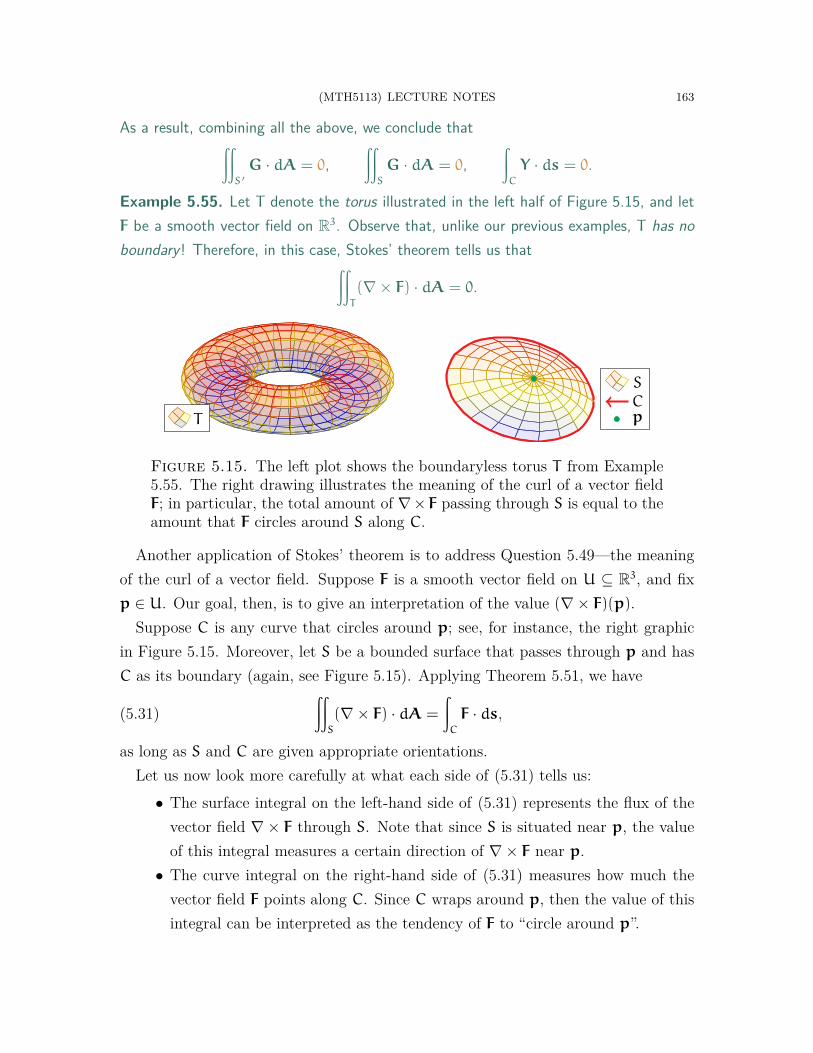
(MTH5113) LECTURE NOTES 163
As a result, combining all the above, we conclude that∫∫S ′G · dA = 0,
∫∫S
G · dA = 0,∫C
Y · ds = 0.
Example 5.55. Let T denote the torus illustrated in the left half of Figure 5.15, and letF be a smooth vector field on R3. Observe that, unlike our previous examples, T has noboundary! Therefore, in this case, Stokes’ theorem tells us that∫∫
T
(∇× F) · dA = 0.
T
S
Cp
Figure 5.15. The left plot shows the boundaryless torus T from Example5.55. The right drawing illustrates the meaning of the curl of a vector fieldF; in particular, the total amount of ∇×F passing through S is equal to theamount that F circles around S along C.
Another application of Stokes’ theorem is to address Question 5.49—the meaningof the curl of a vector field. Suppose F is a smooth vector field on U ⊆ R3, and fixp ∈ U. Our goal, then, is to give an interpretation of the value (∇× F)(p).
Suppose C is any curve that circles around p; see, for instance, the right graphicin Figure 5.15. Moreover, let S be a bounded surface that passes through p and hasC as its boundary (again, see Figure 5.15). Applying Theorem 5.51, we have
(5.31)∫∫
S
(∇× F) · dA =
∫C
F · ds,
as long as S and C are given appropriate orientations.Let us now look more carefully at what each side of (5.31) tells us:
• The surface integral on the left-hand side of (5.31) represents the flux of thevector field ∇× F through S. Note that since S is situated near p, the valueof this integral measures a certain direction of ∇× F near p.
• The curve integral on the right-hand side of (5.31) measures how much thevector field F points along C. Since C wraps around p, then the value of thisintegral can be interpreted as the tendency of F to “circle around p”.

164 (MTH5113) LECTURE NOTES
Also, keep in mind that these observations hold for any such curve C and surface S.Thus, from the above, we arrive at the following rough interpretation: (∇× F)(p)
quantifies how, and how much, the vector field F “circles around p” nearby p.
Remark 5.56. In fact, a more careful look at (5.31) yields a more precise conclusion: thecomponent of (∇× F)(p) in any direction X ∈ TpR3 tells us how much F “circles aroundp” nearby p along the plane that is perpendicular to X.
5.8. The Divergence Theorem. Green’s and Stokes’ theorems related integralsover 2-dimensional objects to integrals over their 1-dimensional boundaries. In thenext (and last) integral identity, we again raise the dimension—we connect integralsover 3-dimensional regions to integrals over their 2-dimensional boundaries.
The classical result for this setting is known as the divergence theorem. Its firstversions were primarily attributed to Carl Friedrich Gauss (German mathematicianand physicist, 1777–1855) and Joseph-Louis Lagrange (French-Italian mathematicianand physicist, 1736–1817). (In case you were wondering, “Italian” is not a mistake;Lagrange’s birth name was Giuseppe Luigi Lagrangia.) Others, including GeorgeGreen, have also made contributions toward the theorem in later years.
We now give a precise statement of the divergence theorem:
Theorem 5.57 (Divergence theorem). Let W ⊆ R3 be open and bounded, and assumethe boundary of W consists of a union of surfaces S1, S2, . . . , Sk. In addition, let F be asmooth vector field that is defined on W and its boundary. Then,
(5.32)∫∫∫
W
(∇ · F)dV =
∫∫S1
F · dA+ · · ·+∫∫
Sk
F · dA,
where the surfaces S1, . . . , Sk are given the outward-facing (from W) orientation.
Again, rather than delving into the formal definitions of boundaries and outwardorientations, we instead demonstrate Theorem 5.57 through examples:
Example 5.58. As usual, let S2 denote the unit sphere centred at the origin,
S2 = {(x, y, z) ∈ R3 | x2 + y2 + z2 = 1},
here with the outward-facing orientation, and let B denote the interior of S2,
B = {(x, y, z) ∈ R2 | x2 + y2 + z2 < 1}.
Note that the boundary of B is precisely S2; see the left illustration in Figure 5.16.

(MTH5113) LECTURE NOTES 165
Suppose now that F is the vector field from Example 4.78:
F(x, y, z) = (x, y, z)(x,y,z), (x, y, z) ∈ R3.
Let us now apply the divergence theorem to compute the integral of F over S2.First, using (5.26), we compute
(∇ · F)(x, y, z) = ∂xx+ ∂yy+ ∂zz
= 3.
Applying Theorem 5.57 to the above B and F then yields∫∫S2F · dA =
∫∫∫B
(∇ · F)dV
= 3
∫∫∫B
dV .
In other words, the integral of F over S2 is simply three times the volume of B.Recall that the volume of B, which is a ball of radius 1, is simply 4π
3· 13 = 4π
3. (This
result could be derived with a bit of multivariable calculus—in particular, by changing tospherical coordinates.) As a result, we obtain∫∫
S2F · dA = 3 · 4π
3= 4π,
which is the same answer as was obtained in Example 4.79.
B
S2
W
S3
S1
S2
Figure 5.16. The left illustration shows the setting of Example 5.58, wherethe region B is the inside of the drawn sphere S2. Similarly, the right illus-tration shows the setting of Example 5.59; the region W is the interior ofthe surfaces S1, S2, S3 drawn there. In both graphics, the orientations of theboundary surfaces are represented by purple arrows.
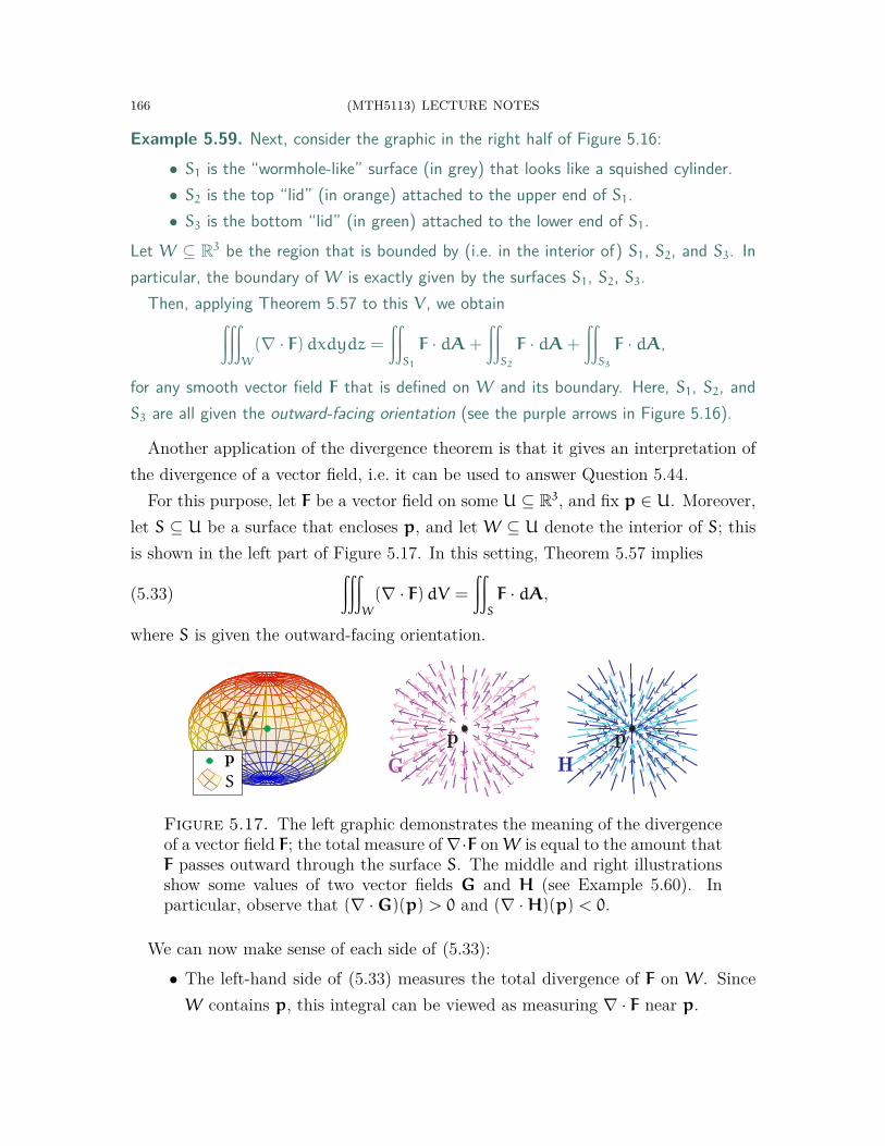
166 (MTH5113) LECTURE NOTES
Example 5.59. Next, consider the graphic in the right half of Figure 5.16:• S1 is the “wormhole-like” surface (in grey) that looks like a squished cylinder.• S2 is the top “lid” (in orange) attached to the upper end of S1.• S3 is the bottom “lid” (in green) attached to the lower end of S1.
Let W ⊆ R3 be the region that is bounded by (i.e. in the interior of) S1, S2, and S3. Inparticular, the boundary of W is exactly given by the surfaces S1, S2, S3.
Then, applying Theorem 5.57 to this V , we obtain∫∫∫W
(∇ · F)dxdydz =∫∫
S1
F · dA+
∫∫S2
F · dA+
∫∫S3
F · dA,
for any smooth vector field F that is defined on W and its boundary. Here, S1, S2, andS3 are all given the outward-facing orientation (see the purple arrows in Figure 5.16).
Another application of the divergence theorem is that it gives an interpretation ofthe divergence of a vector field, i.e. it can be used to answer Question 5.44.
For this purpose, let F be a vector field on some U ⊆ R3, and fix p ∈ U. Moreover,let S ⊆ U be a surface that encloses p, and let W ⊆ U denote the interior of S; thisis shown in the left part of Figure 5.17. In this setting, Theorem 5.57 implies
(5.33)∫∫∫
W
(∇ · F)dV =
∫∫S
F · dA,
where S is given the outward-facing orientation.
WpS
pG
pH
Figure 5.17. The left graphic demonstrates the meaning of the divergenceof a vector field F; the total measure of ∇·F on W is equal to the amount thatF passes outward through the surface S. The middle and right illustrationsshow some values of two vector fields G and H (see Example 5.60). Inparticular, observe that (∇ ·G)(p) > 0 and (∇ ·H)(p) < 0.
We can now make sense of each side of (5.33):• The left-hand side of (5.33) measures the total divergence of F on W. SinceW contains p, this integral can be viewed as measuring ∇ · F near p.
(MTH5113) LECTURE NOTES 167
• The right-hand side of (5.33) measures the outward flux of F through S—thedegree to which the arrows of F are leaving S. Since S encloses p, this can beviewed as a measure of how much F is pointing away from p.
In addition, keep in mind that (5.33) holds for any such surface S and interior W.Thus, the divergence can be roughly interpreted as follows: (∇ · F)(p) quantifies
how much F is “pointing away from p” nearby p. If the values of F near p are pointingaway from p, then (∇ · F)(p) will be positive. On the other hand, if the values of Fnear p are pointing toward p, then (∇ · F)(p) will be negative.
Example 5.60. Consider the middle and right drawings of Figure 5.17, which illustratesome values of two vector fields G (in purple) and H (in blue), respectively.
Now, since the purple arrows in the middle drawing are pointing outward and away fromp, we deduce that (∇ ·G)(p) > 0. Similarly, since the blue arrows in the right drawingare all pointing inward toward p, we thus conclude that (∇ ·H)(p) < 0.
We also note that Theorem 5.57 can be generalised to all dimensions: roughly, foran open and bounded D ⊆ Rn, the integral over D of ∇ · F is equal to the integral ofthe outward normal component of F over the boundary of D. We cannot give a precisestatement of this here, since we have not discussed higher-dimensional geometricobjects. However, we can give a formal statement in the case of n = 2:
Theorem 5.61 (Divergence theorem). Let D ⊆ R2 be open and bounded, and assumethe boundary of D consists of a union of curves C1, C2, . . . , Ck. In addition, let F be asmooth vector field that is defined on D and its boundary. Then,
(5.34)∫∫
D
(∇ · F)dA =
∫C1
(F · n)ds+ · · ·+∫Ck
(F · n)ds,
where n denotes the outward-pointing (from D) unit normal to C1, . . . , Ck.
Remark 5.62. In fact, one can use Theorem 5.61 to prove Theorem 5.29, and vice versa.
Remark 5.63. Moreover, when n = 1, the divergence theorem reduces to (5.15).
Finally, let us mention that there is a general integral theorem that includes all theidentities we have studied—the fundamental theorem of calculus, Green’s theorem,Stokes’ theorem, and the divergence theorem—as special cases. This all-encompassingresult is called the generalised Stokes’ theorem and is most succinctly expressed as
(5.35)∫M
dα =
∫∂M
α.
168 (MTH5113) LECTURE NOTES
Although we certainly do not have the time nor the background to discuss (5.35)in detail, let us at least summarise what every object in (5.35) means:
• M is the n-dimensional geometric object (a manifold) over which we integrate.• ∂M denotes the (n− 1)-dimensional boundary of M.• The integrand α is a special object known as a differential form.• dα denotes a special “derivative” (called an exterior derivative) of α.
The generalised Stokes’ theorem is a topic that one encounters in a more advanceddifferential geometry module. If you continue your studies in geometry and analysis,then you will most likely come across these topics in the future!
5.9. Some Equations of Physics. Historically, Stokes’ theorem and the divergencetheorem have played essential roles in the development of physics.
One well-known example of this comes from classical electromagnetism. For thisdiscussion, we consider two vector fields on R3:
• The electric field E, with E(p) representing the electric force at p.• The magnetic field B, with B(p) representing the magnetic force at p.
Two of the fundamental laws of electromagnetism, from the early 1800s, are as follows:(1) Faraday’s law: The change in time of the magnetic flux through a surface S is
equal, up to sign, to the electric force around its boundary curve C (see theleft graphic in Figure 5.18 for an illustration of S and C):
(5.36) −∂
∂t
∫∫S
B · dA =
∫C
E · ds.
(2) Gauss’s law: The outward electric flux through a closed and bounded surfaceS is equal to the total charge enclosed in the region W inside S:∫∫
S
E · dA = Q(W)(5.37)
=
∫∫∫W
ρdV .
Here, Q(W) denotes the total charge inside W, and ρ represents the chargedensity. (See the right graphic in Figure 5.18 for an illustration.)
Remark 5.64. There are two additional electromagnetic laws—Ampère’s law and Gauss’slaw for magnetism—which have forms similar to (5.36) and (5.37). However, to keep ourdiscussions brief, we restrict our attention only to Faraday’s and Gauss’s laws.

(MTH5113) LECTURE NOTES 169
Remark 5.65. More precisely, the vector fields E and B should also depend on a fourthvariable, t, representing the time. For simplicity, we omit this from the notation.
S
C
W
S
Figure 5.18. The left illustration contains the setting of Faraday’s law,which involves a bounded surface S and its boundary curve C. The rightdrawing shows the setting of Gauss’s law, which involves a closed andbounded surface S along with the region W enclosed by S.
Applying Stokes’ theorem to the right-hand side of Faraday’s law, (5.36), we obtain
(5.38) −∂
∂t
∫∫S
B · dA =
∫∫S
(∇× E) · dA,
for any such bounded surface S ⊆ R3. Similarly, applying the divergence theorem tothe left-hand side of Gauss’s law, (5.37), yields the integral identity
(5.39)∫∫∫
W
(∇ · E)dV =
∫∫∫W
ρdV ,
again for any such region W ⊆ R3.Since (5.38) and (5.39) hold for every possible surface S and region W, one can,
in fact, conclude that the integrands in these identities are equal to each other. (Werefrain from giving a proof of this here.) This results in the differential identities,
(5.40) −∂
∂tB = ∇× E, ∇ · E = ρ,
which are two of the four Maxwell’s equations. (The other two equations are similarlyobtained using Ampère’s law and Gauss’s law for magnetism.)
The equalities in (5.40) are examples of partial differential equations. One advan-tage of writing the laws of electromagnetism in this differential form is that one canproceed to solve these equations for E and B, for all positions and times. This allowsone to predict the future behaviours of our electric and magnetic fields.
Remark 5.66. If you are interested in partial differential equations, then you shouldcertainly consider the third year module MTH6151: Partial Differential Equations.

170 (MTH5113) LECTURE NOTES
As an additional example, we play a similar game with fluid mechanics. Supposewe have a fluid, which we mathematically model using the following:
• A scalar function ρ : R3 → R, with each value ρ(x, y, z) representing the massdensity of the fluid particle at position (x, y, z).
• A vector field v on R3, such that each tangent vector v(x, y, z) represents thevelocity of the fluid particle at position (x, y, z).
In particular, the total mass of the fluid within a bounded region W ⊆ R3 is given by
M(W) =
∫∫∫W
ρdV .
Now, the guiding physical principle in our discussion is the following:
• Continuity equation: The rate of change of the mass of the fluid in a regionW ⊆ R3 is equal to the total flux of the fluid into W through its boundary S:
(5.41) ∂
∂t
∫∫∫W
ρdV = −
∫∫S
ρv · dA.
Note the left-hand side of (5.41) indeed captures the change in the total fluid massin W. In the right-hand side, S is given the outward-facing (from W) orientation,hence the total fluid flow into W is given by the negative of the flux integral throughS. See Figure 5.19 for an illustration of the setting of (5.41).
W
S
Figure 5.19. The illustration shows a fluid flowing out of a spherical regionW through its boundary surface S; this is indicated by purple arrows. As aresult of this, the total mass of the fluid in W is decreasing.
(MTH5113) LECTURE NOTES 171
One interpretion of (5.41) is as a statement of mass conservation: fluid particlescannot instantaneously “teleport” from one point to another. Instead, the only waythat such a particle can enter or leave W is to pass through its boundary S.
Remark 5.67. Again, to be more precise, both ρ and v should depend on an additionaltime variable, which we omit from our notations for simplicity.
Applying the divergence theorem to the right-hand side of (5.41) yields∂
∂t
∫∫∫W
ρdV = −
∫∫∫W
[∇ · (ρv)]dV .
(Recall that S is given the outward-facing orientation.) Since the above holds forevery region W, we conclude from this the following differential identity:
(5.42) −∂
∂tρ = ∇ · (ρv).
The equation (5.42) is yet another example of a partial differential equation thatplays an important role in research within mathematics, physics, and engineering. Inparticular, this equation can be solved to predict future behaviours of fluids.

172 (MTH5113) LECTURE NOTES
Notes and Acknowledgments
MTH5113: Introduction to Differential Geometry was designed from the topics oftwo previously existing modules, MTH5102: Calculus III and MTH5109: GeometryII: Knots and Surfaces. One goal of MTH5113 was to better streamline the contentsof MTH5102 and MTH5109, which had significant overlaps.
The present notes are a lightly updated version of the MTH5113 lecture notes fromprevious years. The most recent changes include the following:
• A new section (2.4: Limits and Continuity) was added to provide an informaldiscussion on continuous vector-valued functions. This was done to make theformal definitions of curves and surfaces more understandable.
• The discussions in a few sections were made more concise.I thank the students from the previous iterations of MTH5113 for their feedback onthe module contents and on the lecture notes.
The contents of these lecture notes are largely based on the following sources:• Previous lecture notes [3, 5, 6] for MTH5109.• Previous lecture notes [2] for MTH5102.
However, I do regret that several interesting topics from these notes (in particular,the curvature of curves and surfaces) could not be covered in MTH5113. Hopefully,these will be found in third-year modules in the future.
While these notes are intended to be entirely self-contained, the interested readermay also wish to consult the following texts from the official module reading list:
(1) Thomas, Weir, Hass. Thomas’ Calculus. [10].(2) Spiegel, Lipschutz, Spellman. Vector Analysis and an Introduction to Tensor
Analysis. [9].(3) Simons. Vector Analysis for Mathematicians, Scientists and Engineers. [8].(4) Bär. Elementary Differential Geometry. [1].(5) Pressley. Elementary Differential Geometry. [4].
These texts contain material related to and beyond what is covered by these notes.
(MTH5113) LECTURE NOTES 173
References
1. C. Bär, Elementary Differential Geometry, Cambridge University Press, 2010.2. M. MacCallum, C. D. Murray, P. Saha, W. Sutherland, and M. J. Thompson,
MTH5102 (Calculus III) Lecture Notes, 2010, Queen Mary University of London.3. S. Majid, MTH5109 (Geometry II) Lecture Notes, 2015–2016, Queen Mary University of
London.4. A. Pressley, Elementary Differential Geometry, Springer, 2010.5. A. Shao, MTH5109 (Geometry II) Lecture Notes, 2016–2017, Queen Mary University of
London.6. , MTH5109 (Geometry II) Lecture Notes, 2017–2018, Queen Mary University of
London.7. , MTH5109 (Introduction to Differential Geometry) Lecture Notes, 2018–2019, Queen
Mary University of London.8. S. Simons, Vector analysis and an introduction to tensor analysis, Pergamon, 1970.9. M. R. Spiegel, S. Lipschutz, and D. Spellman, Vector analysis and an introduction to tensor
analysis, McGraw-Hill, 2009.10. G. B. Thomas, M. D. Weir, and J. Hass, Thomas’ calculus, Addison-Wesley, 2010.11. Wikipedia: Geometry,
http://en.wikipedia.org/wiki/Geometry.