Ceophys. J . Int. (1991) 105, 119-130

2-D reflectivity method and synthetic seismograms for irregularly layered structures-11. Invariant embedding approach

K. Koketsu,’* B. L. N. Kennett’ and H. Takenaka2 ’ Research School of Earth Sciences, Australian National University, GPO Box 4, Canberra ACT 2601, Australia

Obayashi Corporation Technical Research Institute, Shimokiyoto 4-640, Kiyose-shi, Tokyo 204, Japan

Accepted 1990 October 3. Received 1990 August 31; in original form 1990 May 16

SUMMARY Laterally varying interfaces cause coupling between wavenumbers so that seismo- grams in two-dimensionally layered media can be synthesized by means of ‘supermatrices’, which include the coupled contributions of all the wavenumbers. We introduce reflection and transmission ‘supennatrices’ in order to eliminate numerical problems arising from loss of precision for evanescent waves in the seismogram synthesis. An interface is assumed to be such that the reflected and transmitted wavefields on its two sides can be represented as purely upgoing and downgoing waves, i.e. the Rayleigh ansatz is imposed. The computational demands of this method can be kept to a minimum by exploiting propagation invariants in the coupled wavenumber domain.

The superior performance of this ‘invariant embedding’ approach when compared to propagator or finite difference schemes is illustrated by application to the response of sedimentary basins to excitation by an incident plane wave or a line force. The results are in good general agreement with the other methods, but show greater numerical stability and computational efficiency. In the case of a single interface the ‘invariant embedding’ procedure for P-SV-waves takes 45 per cent less computation time and 29 per cent less memory than the propagator method of Koketsu (1987a,b). The gains are reduced in a multilayer case because of the level of computation required to calculate the addition rules for the large reflection and transmission supermatrices.

Key words: irregular layering, propagation invariant, synthetic siesmograms.

1 INTRODUCTION

A wide range of theoretical studies have being carried out over the last 20 years with the object of synthesizing seismograms in irregularly layered media. Many authors have tried to match the boundary conditions of irregular interfaces by superposition of the known solutions in a homogeneous layer. If the solution u ( x ) in an irregularly layered medium is represented as a linear combination of the homogeneous solutions $,(x) ,

the matching of the boundary condition B(u) = 0 can be accomplished with ‘the method of weighted residuals’ (Finlayson 1972; Fletcher 1984). The weighting factors an,

* On leave from: Earthquake Research Institute, University of Tokyo, Tokyo 113, Japan.

n = 1, 2 , . . . , N are to be determined by solving the simultaneous equations

N

IWk(.)B[ n = l 2 a,$”(x)] dS = 0, k = 1,2 , . . . , (1.2)

where w&) is a weighting function which samples the boundary condition on the interface S. The following functions are usually used for weighting:

wk(x) = 6 ( x - x k ) (collocation matching),

= 4k(X) (Galerkin matching). (1.3)

= aB/da , (least-squares matching),

From Huyghens’ principle, the Green’s functions for point-sources distributed on the interface are most appropriate as a trial function &,(x), and these are imposed in the Boundary Integral Equation Method (BIEM). Sbnchez-Sesma & Esquivel (1979) and Dravinski (1983) computed SH spectra scattered by an irregular interface

119

120 K . Koketsu, B. L. N . Kennett and H . Takenaka

with the collocation BIEM. Stinchez-Sesma, Herrera & AvilCs (1982) used the least-squares BIEM for the same problem. Campillo & Bouchon (1985) computed scattered excitation by a line-source with the finite Fourier expansion (‘discrete wavenumber representation’) of the Green’s function and collocation matching. The Boundary Element Method (BEM) looks quite different from BIEM, but it is also based on a similar concept (Brebbia 1978), and Kawase (1988) computed scattered P-SV-waves using BEM.

However, computation based on the use of the Green’s functions is very complicated and time consuming. If we can synthesize seismograms by using only homogeneous plane waves, the computation would become simple and fast. Aki & Larner (1970) showed that this approach should be valid when we rely on the Rayleigh amatz, i.e. an upgoing wavefield can be neglected in the lowermost half-space of an irregularly layered medium. Because of coupling between wavenumbers caused by an irregular interface they considered all the wavenumbers together. To handle this coupling Koketsu (1987a) introduced ‘superpropagators’ (Haines 1988), whose entries are the well-known single- wavenumber propagators, and extended Aki & Larner’s formulation to multilayered media. A more complete development of this formulation appears in Koketsu (1987b), including P-SV interactions. Later, Geli, Bard & Jullien (1988) and Horike (1988) independently discovered similar formulations.

Axilrod & Ferguson (1990) reported that the CPU time required for the method of Campillo & Bouchon (1985) is approximately an order of magnitude greater than for this approach. The Boundary Element Method should also require a CPU time with the same order.

The propagator formulation for irregularly layered media is subjected to the class of numerical problems, which beset propagation techniques in horizontally layered media, especially loss of numerical precision for evanescent waves. Takenaka (1990) has shown how the reflection/transmission matrix approach of Kennett (1983) can be adapted to irregularly layered media. This procedure eliminates problems with evanescent waves, but requires a number of large-scale matrix inversions, which introduce a different range of numerical complications.

In this paper we will present an alternative formulation of the reflection/transmission matrix approach, which exploits the propagation invariants of Kennett, Koketsu & Haines (1990) to simplify the calculations. This new method will be called ‘invariant embedding’ based on the nomenclature in the review paper of Chin, Hedstrom & Thigpen (1984). We demonstrate the superior numerical stability and computa- tional efficiency of the invariant embedding technique compared with the propagator formulation using a variety of numerical examples. In order to provide a clear link to the reflection and transmission results the notation used is based on Kennett (1983) rather than that of Koketsu (1987a,b).

2 IRREGULAR INTERFACES

We consider layered media with two-dimensionally varying interfaces. We take a Cartesian coordinate system ( x , y, z ) with z-axis taken positive downward, and assume that the free surface and interfaces vary in the x - z plane. Therefore the wavefield and media do not depend on the coordinate y.

We will assume a time dependence exp(iot), but will not normally represent the time variation explicitly.

In a homogeneous and isotropic layer having P-wave velocity a, S-wave velocity /3 and density p , the displacement can be expressed as

u(x, z ) = [u(x, z) , w ( x , z ) , u(x, Z)IT

in terms of P, S V and SH contributions (note that we locate u at the last element to isolate the SH contribution). When we take Fourier transforms with respect to x

f(k, z) = I + - f ( x , z)e-’” dx, -m

(2.1) has harmonic solutions in the k (horizontal wavenumber) domain

4(k, z ) = exp (fiv,z), $(k, z ) = exp (*iv,z), (2.3) D(k, z ) = exp (rtiv,z),

where

v, = (k; - kZ)’” (k, = w / c , c = a or p ) (2.4)

is a vertical wavenumber. We can then write general solutions with weighting factors Pu,D, S,,D and Hu.D as

+(k, z ) = P U ~ p exp (+iv,z) + P D ~ p exp (-iv,z),

+(k, z) = S ~ E ~ exp(+ivaz) + S ~ E ~ exp (-ivaz), (2.5) 6(k , z) = H , E ~ exp (+iv,z) + H D ~ H exp (-ivpz).

We have a free choice of the scaling parameters E ~ , E~ and E~ in (2.5), because they affect only the physical meanings of the quantities Pu.D, Su,D and Hu,D (Kennett 1983, chapter 3).

vu.D = [Pu,I, exp (fiv,Z), Su,D exp (* iv~z) ,

We define the upgoing and downgoing wave vectors as

Hu,D exp (fivsz)lT (2.6)

and insert (2.5) into the Fourier transform of (2.1). Then we have

u(k, z) = [ii(k, z), *(k, z), D(k, z)lT = MoUuu+ WDvD (2.7)

where

( 0 &H i). (2.8) @,,,(k) = fiv,Ep ikES

Similarly, by using the stress-strain relation we find that

ikEp TivsEs

w t 2) = [f&, z ) , fX2(k z), fXJk z)J’

t , ( k , z> = [fA, z), f , ,(k, z ) , t z y ( k , Z)lT (2.9)

= R U v U + @DUD I

= e U v U + @ D v D ?

where prEp f 2pkvpzS

0 (2.10)

2 - 0 reflectiuity method (11) 121

: ), T 2pkv,~p - p k s

Xu,&) = P b 2PkVi?&S

r = 2v:- k;, 1 = 2k2 - k;. (2.11)

( 0 0 f ipvsEn with

The form of the matrices in (2.8) and (2.10) shows the decoupling between the P-SV-wavefield (Pu, D , Su,D) and the SH-wavefield (Hu,D) in homogeneous layers. We note that

[@J,DD(-k)lTeU,D(k) - [eU,D(-k)]TMU,D(k) 0 (2.12) and

[@d-k)lTKU(k) - “!D(-k)lTMU(k) = -[W%-k)lTNLJ(k) + P%4) lTMD(k) = diag (2ipk;v,&, 2ipk;vi?& 2ipvP&). (2.13)

To simplify the subsequent development we take

cp = (2&v,)-”*, E~ = ( 2 p k i ~ ~ ) - ’ / ~ , cH = ( ~ , U V ~ ) - ” ~ ,

(2.14)

so that (2.13) is further reduced to an imaginary identity matrix.

Consider now layers A and B separated by an irregular interface with the shape controlled by

z(x) = 20 + h(x), (2.15)

which fluctuates around the reference level zo (Fig. 1). The boundary condition of welded contact at the interface z(x) requires the continuity of the displacement u[x, z(x)] and the traction ~ ( x , z(x)] across the interface. In terms of the wavenumber components we need

{ i [ k , z(x)], i [k , z(x)]}’eik” dk (2.16)

to be continuous to satisfy these two interface conditions. We assume that the wavefield on the two sides of the irregular interface can be represented by the homogeneous solutions (2.3). Then, inserting (2.7) into the displacement part of (2.16) and redefining the wave vectors to leave only x-independent terms, i.e.

u U , D ( k ) = [ p U , D exp (*ivmzO)> sU,D exp (*iv~zO)* H U , , exp (*ivazo)lT, (2.17)

we obtain

ii[k, z(x)]e’” dk = I [MU(x, k)uu(k)

+ M&, k)v,(k)l dk (2.18)

where

Mu,D(xt k ) = M“U.D(k)~U.D[h(x)le’”, (2.19) EU,&) = diag [exp (fiv,z), exp (*ivi?z), exp (kivaz)].

On the other hand, by taking n = [n,(x), n,(x)lT as the unit normal to the interface, the traction can be derived from the stress as

t (x , 2) = n,(x)r,(x, 2 ) + n,(x)r,(x, 2). (2.20)

A

n = In,, n,I

Fire 1. An irregular interface between layers A and B. n is the unit normal to the interface.

Inserting this expression and (2.9) into the traction part of (2.16) we get

j i[k, z(x)]e’” dk = j [Nu(x , k)uu(k) + N&, k)u,(k)] dk,

(2.21)

where

Nu,&* k) = [ ~ x ( x ) ~ u , D ( k ) + n, ( - d e u , D(k) lE , D P (x)le’”. (2.22)

We note that

n,(x) = -h ’ / ( l + h”)ln, n,(x) = 1/(1 + h‘2)112, (2.23)

where h’=dh(x ) /dx , and Kennett (1972) found that 1/(1+ h”)ln is common to the traction forms in both layers A and B. Thus we can omit this factor from Nu.D(x, k) and set

k, = [-h’(x)eU,D(k) + ~U,D(k) lEU.D[h(x) le i~ . (2.24)

Mu,D in (2.19) and Nu,D in (2.24) keep the same matrix form as @u,D,@u,D and @u,D so that the decoupling between P-SV- and SH-waves is still valid even in two-dimensionally layered media.

The boundary condition of continuity of displacement and traction can now be written as

IDA(.> k)v,(k) dk = / D B ( X , k)v*(k) dk, (2.25)

where D(x, k ) and u(k) are a pseudo-eigenvector matrix and a total vector defined as

(2.26)

If the interface is flat, i.e. h(x) = 0, the integrands in (2.25) are independent of x except for eik, and the integral equation (2.25) will simply be solved as

(2.27)

For an irregular interface, however, we have no trivial solutions like (2.27). In other words, scattering by the irregular interface causes the coupling between different wavenumbers so that we have to consider all the wavenumbers together.

In order to solve the integral equation (2.25) we first

122 K . Koketsu, B.L. N . Kennett and H . Takenaka

replace the infinite integrals with finite sums (‘a discrete wavenumber representation’) and set

b ( x , k)u(k ) dk = D(x, ki)u(ki) (2.28)

where D includes dk on the right-hand side. We next introduce the total wave ‘supervector’ v and the continuous ‘supermatrix’ D(x) whose entries for wavenumber ki are just u(ki ) and D(x, k;). We can then express (2.25) as

DA(x)vA = D B ( x ) v B * (2.29)

(2.29) represents the boundary condition on the irregular interface (2.15) as a set of continuous equations in terms of x , but can be discretized by using a weighting scheme as in (1.3). For example, using collocation matching we get

D,(X,)V, = D,(x,)v,, (2.30)

However, Aki & Lamer (1970) adopted a slightly different approach: they took the Fourier transform (2.2) of the both sides of (2.29) with respect to a set of wavenumbers and so derived

DA(kj)vA = DB(kj)vB, (2.31)

By introducing the discrete supermatrix D in the coupled wavenumber domain, whose entry for kj is D(k j ) , we rewrite (2.31) as

DAvA = DBvB. (2.32)

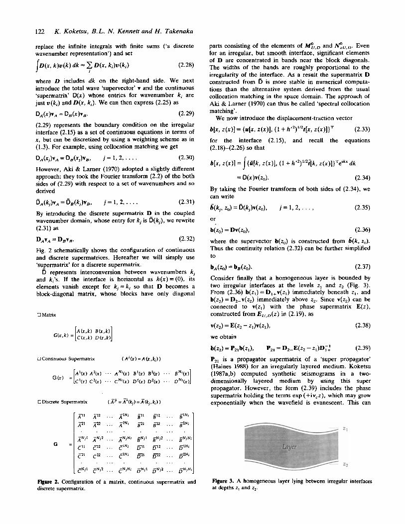
Fig. 2 schematically shows the configuration of continuous and discrete supermatrices. Hereafter we will simply use ‘supermatrix’ for a discrete supermatrix.

b represents interconversion between wavenumbers kj and k,’s. If the interface is horizontal as h ( x ) =(O), its elements vanish except for kj = ki so that D becomes a block-diagonal matrix, whose blocks have only diagonal

i

j = 1,2, . . . .

j = 1,2, . . . .

0 Matrix

0 Continuous Supermatrix ( A Y X ) = A c r , ~ )

0 Discrete Supermatrix ( xj = A ’ ( k j ) = x ( k j , ki) )

G =

F i i 2. Configuration of a matrix, continuous supermatrix and discrete supermatrix.

parts consisting of the elements of w,,, and eu,D. Even for an irregular, but smooth interface, significant elements of D are concentrated in bands near the block diagonals. The widths of the bands are roughly proportional to the irregularity of the interface. As a result the supermatrix D constructed from D is more stable in numerical computa- tions than the alternative system derived from the usual collocation matching in the space domain. The approach of Aki & Larner (1970) can thus be called ‘spectral collocation matching’.

b[x, z(x)] = {u[x, z (x ) ] , (1 + h ’ y t [ x , z(X)]}= (2.33)

for the interface (2.15), and recall the equations (2.18)-(2.26) so that

b[x , z ( x ) ] = / { L [ k , z ( x ) ] , (1 + h’2)1’2i[k, ~ ( x ) ] } ~ e ’ * ~ dk

We now introduce the displacement-traction vector

= D(x)v(zo). (2.34)

By taking the Fourier transform of both sides of (2.34), we can write

&kj, q,) = D(kj)v(zo), (2.35)

or

j = 1, 2, . . . ,

b(Z0) = DV(Z0)l (2.36)

where the supervector b(z,) is constructed from b(k , z0). Thus the continuity relation (2.32) can be further simplified to

bA(Z0) = bB(zO)* (2.37)

Consider finally that a homogeneous layer is bounded by two irregular interfaces at the levels L, and z2 (Fig. 3). From (2.36) b(z,) = D,+v(z,) immediately beneath zlr and b(zZ) = D,-v(z,) immediately above z2. Since v(z2) can be connected to v(zJ with the phase supermatrix E(z), constructed from E,,,(z) in (2.19), as

v ( 4 = E(Z2 - Z M Z l ) ,

we obtain

b(zJ = PZlb(zJr Pz,= Dz-E(z2 - zi)D;: (2.39)

P2, is a propagator supermatrix of a ‘super propagator’ (Haines 1988) for an irregularly layered medium. Koketsu (1987a,b) computed synthetic seismograms in a two- dimensionally layered medium by using this super propagator. However, the form (2.39) includes the phase supermatrix holding the terms exp (+iv,z), which may grow exponentially when the wavefield is evanescent. This can

(2.38)

F i i 3. A homogeneous layer lying between irregular interfaces at depths z, and 2,.

2-0 reflectivily method (ZZ) 123

lead to numerical instability in case of high frequencies, low phase velocities or thick layers. In addition it is necessary to compute a full inverse of D. D is 8Ni x 8N, for P-SV-waves, or 4Ni x 4Nj for SH-waves (Ni , j = the number of wavenum- bers ki, ,) . Such a large-scale matrix inversion may cause computational inaccuracy even if D is nearly block- diagonal.

3 REFLECTION, TRANSMISSION A N D INVARIANTS

For horizontally layered media Kennett (1983) has shown that the exponentially growing terms can be avoided if we formulate the wavefield in terms of the reflection and transmission matrices rather than the propagators. Take- naka (1990) has recently extended this approach to irregularly layered media by direct analogy with the flat interface results of Kennett (1983), but with substantially higher dimensionality.

Consider an incident downgoing wave from the layer A into the layer B through an irregular interface (Fig. 4a). This will give a reflected upgoing wave in A and transmitted downgoing wave in B. If we rely on the Rayleigh ansatz (see e.g. Aki & Richards 1980, chapter 13), there will be no upgoing wave in B. We partition the pseudo-eigenvector

(2.26): supermatrix D and the total wave supervector v as in

and then rewrite boundary condition (2.32) as

(3.2)

By defining the reflection and transmission supermatrices RD, TD to connect the partitioned wavefields:

TDVDA

(a) downgoing wave incidence

f l \ .

\ RuvW

(b) upgoing wave incidence

Figure 4. Schematic representation of reflected and transmitted waves due to (a) downgoing or (b) upgoing wave incidence on the irregular interface separating layers A and 8.

we obtain

(Ez: NDA >( I ) = (::: ::I)(:)’ where I and 0 are the identity and zero supermatrices. Similarly, if we consider an incident upgoing wave from B into A (Fig. 4b) and define the supermatrices R,, T, as

(3.4) MDA RD

VDB = R,VUB, VUA = TUVUBI (3.5)

then (2.32) becomes

c: ::;m = iMUB N U B :::)iJ (3.6)

by neglecting the downgoing wavefield in A.

in (3.4) and (3.6) explicitly, and found that

T, = M&SDDMDA,

Takenaka (1990) solved the simultaneous linear equations

RD = M i % d b A , (3.7)

R, = M&SDUMUB, T, = M;&,M,~, where

SDD = -(ADB -AuA)-’(A,A - ADA), SUD = +(&A - ADB)-’(ADB - ADA), S D U = +(ADe - AuA)-’(AUA - A,,), (3.8) SUU= -(AuA - ADE)-’(ADE - A,,),

AU,D = NU, D (MU,

The calculation of Ru,D and Tu,D by the above formulation requires five matrix inversions, i.e. Mi;, M& ME;, MGb and (AUA-ADB)-’. Takenaka (1990) also found the explicit expressions for the continuous supermatrices Au,D(x, k), so then was able to reduce the number of matrix inversions, but, even in this case, three inversions still remain.

Kennett et al. (1990) established a spatial propagation invariant

for two elastic displacement fields u1 and u2 and their associated traction fields c1 and t2. This will be invariant for any surface spanning the x-y plane in a laterally heterogeneous and anisotropic medium. If we take the interface z ( x ) = r, + h ( x ) in a two-dimensionally layered medium as S, dS = (1 + h12)’’’ dr, so that (3.9) yields

(3.10)

If we assume the interchangeability of integrals, we can note that

=‘I/ dk’ dkf(k’ )g(k)b(k’ + k ) 2Jc

= - / f ( - k ) g ( k ) 1 - dk. 2n (3.11)

124 K. Koketsu, B. L. N . Kennett and H . Takenaka

G =

By using (3.11) and replacing the infinite integral with a finite sum (‘a discrete wavenumber representation’) we rewrite the invariant (3.10) as

c-N:N c-N,-N+I . . _ c-N,O . . . G-N,N-I c - N , N

c -N+I , -N ~ - N t l . - N + l . , . c -N+l ,O . . . G-Nt1.N-I G-Nt1.N

. . . . . . . . c0.A’ cO.-N+~ . , , GO,O , , . c 0 . N - I c 0 . N

. . . , . . . . GN-1,-N GN-I.-N+I . , , GN-1.0 . , . GN-l ,N- I GN-I ,N

c N , - N c N . - N + l _ . . GN,O . . . c N , N - I G N S J

(3.12)

GY =

where N is a supermatrix made from N. The operator #, which was first introduced by Haines

(1988), performs transposition of a supervector or supermatrix and switches the sign of the wavenumbers for their elements. All the supermatrices appearing in this paper have a partitioned form such as

GN.N GN-1.N , , . c 0 . N . . . c - N + l , N c - N , N - GN.N-1 GN-l,N-I . , . c0.N-1 . . . G-NLLN-I c - N . N - l

. . . . . . . ,

c N . 0 GN-1.0 . . . ~ 0 . 0 . . . G-N+I,O c - N . 0

. . . . . . . ,

GN;Ntl c N - I . - N + I . . . cO,-N+I , . , G-N+I,-N+I c - N , - N + l

cN:N GN-I -N , , . GO,-N , , , c-N+I,-N c-N.-N

(3.13)

G’ can be also partitioned after transposition with the operator # as

(3.14)

When we define the Fourier transform as in (2.2) and discretize it with an equal interval A k , supervectors and the partitions of supermatrices have the forms illustrated in Fig. 5(a). Since they include g ( - i A k ) and G ( - j A k , - i A k ) as well as g( iAk) and G ( i A k , j A k ) , we can construct g” and G* by just rearranging the elements of g and G . g” is the reflected image of gT about the line ki = 0. G” is that of G about the line ki + k, = O (Fig. Sb), which is the alternate diagonal of G to the line ki = ki (the reflection line of GT). Therefore, the operator # has similar characteristics to

(a) Supervector and Partition of Supermatrix ( 8 ’ = g ( i h k ) , G ’ J =G(iAk,jAk))

(b) Transposed

z(x) = 20 + h(x)

Fire 6. Two spanning surfaces close to the interface z ( x ) = z, + h(x) . S, is a horizontal plane immediately above z,, while & is located on the S, side along the interface.

those of the transpose operator T:

(G”)” = G , (GH)* = H*G*, (G-’)* = (G#)-’. (3.15)

These relations are valid not only for the partitions of supermatrices but also for supermatrices themselves.

In the previous section we have already established the upgoing and downgoing wavefields as u1 and u2 in an irregularly layered medium. Thus, from (2.36) and (3.1) we find that the supervectors of up and downgoing waves

(3.16)

work as b, and b2 in (3.12). We now construct some useful identities for solving (3.4) and (3.6) by means of the invariant (3.12) and the wavefields (3.16). Consider two surfaces S, and S, spanning the x-y plane close to an irregular interface at the level 2,. S, is a horizontal plane immediately above G, while S, is located on the S, side along the interface (Fig. 6). If we take b, = b, = bu,

where

( B1, B2) = B7NB2 = MfN2 - NYM,. (3.18)

Since S, is horizontal, Mu and Nu on S, are block-diagonal supermatrices, whose entries are the elements of Pu and xu. By recalling (2.12), i.e.

we find that every entry of (Bu, B,) vanishes on S,. This argument is also valid in the case of b, = b2 = bD, so that on s, (B,, B,) = (BD, B,) =O. (3.19)

In a similar way from (2.13) and (2.14) we obtain another identity on S,:

(BD, B,) -(Bu, B,) = i l . (3.20)

Meanwhile, b7Nb2 is invariant at any surface spanning the x-y plane, so that

vE,D((Bu,D, BU,D)*- (Bu.D, BU,D)S1)vu.D =O, V Z ( ( B U ? B D ) s * - (BU? B D M V D (3.21)

=VZ((BD, BU)*- (BD, BU).S,)vU=O.

Since (3.21) has to be satisfied for arbitrary supervectors v ~ . ~ , the identities (3.19) and (3.20) should be valid even on S, along the irregular interface.

These identities mean that suitable choice of B in forming an invariant with the two sides of (3.4) or (3.6) can readily

2-0 reflectivity method ( I I ) 125

extract either R,,, or T,,,. Firstly, (3.4) multiplied by

leads to

(3.22)

(3.23)

(3.24)

(3.25)

(3.26)

and so only a single matrix, i.e. (B,,, BOA) need be inverted to generate R,,, and Tu.D. Besides (BDB, BUA) is just 4Ni X4Ni for P-SV-waves or 2Ni X2Ni for SH-waves, while a super propagator D is 8Ni X 8Ni or 4Ni X 4Ni.

The above calculation of R,,, and T,,, may sometimes be numerically unstable for the normalization (2.14) due to the influence of the complex roots. Therefore we first calculate &,, and T,, without this normalization, and then obtain R,,D and Tu.D by

R, = E~'&,E,, (3.27) R, = E;'&,E~,

where is a block-diagonal supermatrix consisting of E ~ , E, and E~ in (2.14) for the layer A or B.

When we compare (3.24) and (3.25) with (5.19) and (5.24) in Kennett (1983), we find that T,,, has an opposite sign to the corresponding transmission 'matrix' for a horizontally layered medium. This is due to a subtle difference in the definitions of Mu,, and Nzu,,. We defined them in (2.7) and (2.9) as matrices connecting potential amplitudes to displacements and stresses, while Kennett (1983) regarded them as eigenvector matrices of the equation of motion. However, by following the procedure in chapter 5 of Kennett (1983) we can prove the symmetries

R, = Rg, R, = RE, T, = Tg, (3.28)

which are very similar to (5.60) in his book. The direct analogy with the results for horizontally

layered media (Kennett 1983, chapter 6 ) means that we can find the reflection and transmission supermatrices for a region (zA, zc) in terms of the supermatrices for the subregions (zA, zB) and (zB, zC):

RA,c = RGB + T$BRgc[I - R$BRgq-lT$B,

T, = E;''€,E~',

To = E;'T,E;',

cc = TgcC(I - R$BRgc]-'PDB, (3.29) R t C = REc + TECRcB[I - RgcR$B]-'TEc,

Ec = PUBII - RgcRA,B]-'TEc.

These addition rules include two supermatrix inversions, i.e. (I - R$BRgc)-l and (I - RgcR$B)-', but one of them can be calculated from the other by using

(I - R ~ ~ R A , ~ ) = (I - R $ ~ R ~ ~ ) * " . (3.30)

For example we consider the case of the homogeneous layer lying between irregular interfaces illustrated in Fig. 3 as a single element of an irregularly layered medium. We suppose the reflection and transmission supermatrices at zz- are known and write e.g. RD(z2-). Since the reflection and transmission supermatrices in the homogeneous layer are simply given by

R,=R,=O, T,=TU=E,, 12 (3.31)

where EE is a downgoing part of the phase supermatrix E(z2 - zl), we can express the reflection and transmission supermatrices at z,+ as

Ru(rl+) = E ~ R , ( z , - ) E ~ , R,(z,+) = E:R,(Z,-)E~, T,(z,+) = T,(z , - )E~,

Tu(zl+) = EL9,(z2-). (3.32)

The upgoing phase term exp (+ivcz) never appears in (3.32) so that the computation for Ru,D and T,,, does not suffer exponential overflows.

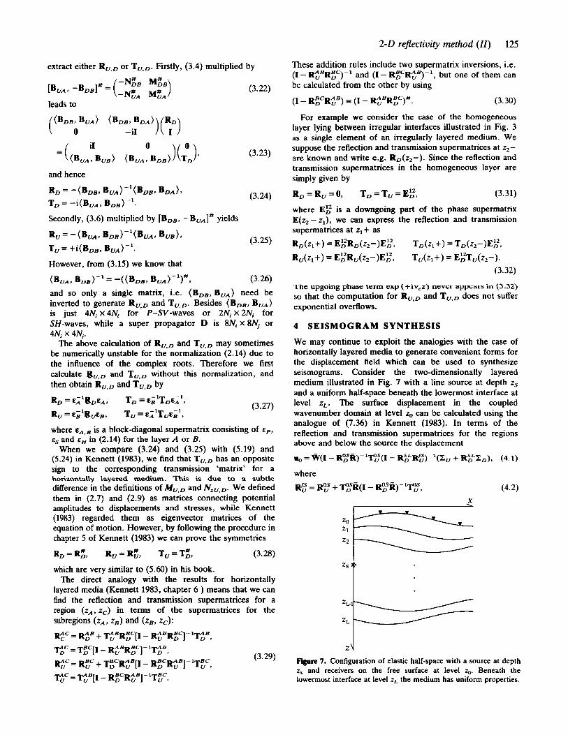
4 SEISMOGRAM SYNTHESIS We may continue to exploit the analogies with the case of horizontally layered media to generate convenient forms for the displacement field which can be used to synthesize seismograms. Consider the two-dimensionally layered medium illustrated in Fig. 7 with a line source at depth z, and a uniform half-space beneath the lowermost interface at level zL. The surface displacement in the coupled wavenumber domain at level r, can be calculated using the analogue of (7.36) in Kennett (1983). In terms of the reflection and transmission supermatrices for the regions above and below the source the displacement

U, = W(I - ~gR)-lP;(i - R","R~)-~(x, + RS,~,), (4.1) where

(4.2) RC = R F + T";R(I - RER)-'F,S, X

%we 7. Configuration of elastic half-space with a source at depth z, and receivers on the free surface at level q,. Beneath the lowermost interface at level zL the medium has uniform properties.

126 K . Koketsu, B. L. N . Kennett and H . Takenaka

and Zu,D represents the upgoing or downgoing part of the jump supervector due _‘o the source. The free-surface reflection supermatrix R and the surface amplification supermatrix W are defined by

1 = -N;;N,, w = M, + M ~ R . (4.3)

These quantities are best calculated in unnormalized form, and the normalization supermatrix E,, can be applied to give

R = GIRE,,, w = Wk. (4.4) The recursive application of the addition rules (3.29) allows us to calculate Ru,n and TU,D in the subregions (q,, zs) and (zs, I=), where an arbitrary number of layers may exist.

By means of (4.1) we can construct the response to a two-dimensionally layered medium in the transform domain, as a function of frequency w and wavenumber k. To get synthetic seismograms we numerically invert the transforms.

We now show a variety of numerical examples to demonstrate the superior performance of our new invariant embedding approach compared with the propagator technique (Koketsu 1987a,b). First we calculate the seismic response of a layered sedimentary basin to an incident plane wave. In this case z, = zL and Z, = 0. We can then calculate the surface displacement using

u, = W[I - RgR]-’p;Zu. (4.5)

The first example is the simplest one where a uniform basin (a = 1.4 km s-’, B = 0.7 km s-’, p = 2.0 g cm-’) lies above a half-space (a = 6.06 km s-’, /3 = 3.5 km s - ’ , p = 3.3gcrf3) with a vertically incident SH-wave. This is a

(km) SH (y) -Invariant Embedding --- Propagator -Finite Difference

0 20 50

0 50 , 100 150 (sec)

Figue 8. The y-component response of a uniform sedimentary basin to a vertically incident SH-wave on the free surface. The basin shown on the upper right side has an asymmetric shape and sharp corners.

variation of the well-known test case introduced by Boore, Larner & Aki (1971), but the interface has an asymmetrical shape with sharp comers. The depth of the basin h ( x ) vanes from 1 km at the edge to 6 km near the centre:

h ( x ) = D + (C/W,)X, x 5 ~ 1 ,

= D + (C/W,)(W, + w Z - X ) , ~1 < X < W, + w,, (4.6)

where D = 1 km, C = 5 km, w, = 20 km and w, = 30 km. Fig. 8 displays the y-component seismograms at the top of the basin calculated by three different methods with a common incident waveform of Ricker type

(4.7)

where b = n(t - t,)/t,,, t, = 20 s and t, = 18.3 s. The ‘finite difference’ solution was calculated using the

scheme described by Yamanaka, Seo & Samano (1989) in the time domain, while the ‘propagator’ solution was calculated using the super propagators in (2.39) and the method developed by Koketsu (1987a). The ‘invariant embedding’ approach makes use of our development in this paper. The three results agree well and it is difficult to detect any difference between the invariant embedding and propagator results. At later times the differences in the finite difference solutions arise from cumulative delays due to nhmerical dispersion. As pointed out by Bard & Bouchon (1980), the two edges of the basin generate Love waves, which travel laterally and are reflected at the opposite slopes. These correspond to major later arrivals in the seismograms.

On the Fujitsu VP-100 of the ANU Supercomputer Facility, the calculations for Fig. 8 took 12.68s for the invariant embedding method (IE), 16.95 s for the propaga- tor technique (PR) and over 30min for the finite difference code (FD). Since computing performance should depend on the Fujitsu compiler and our coding capability, we kept the same coding style and took the same values for computation parameters, such as sampling numbers and discretizing intervals etc., between IE and PR as far as possible (see Table 1). All the FFTs and matrix inversions were carried out using vector-oriented subroutines supplied by Fu jitsu. FD shows poor performance partly because of the low vectorization of its codes (compare the W U time to the CPU time on Table 2).

The VP-100 is running under an MVS/XA-compatible operating system, which supports extended memory above the 16 Mbytes boundary of basic memory. IE occupied basic memory of 340Kbytes (KB) plus extended memory of 604KB. These values are 18 per cent less than the total memory occupation of PR, and 70 per cent less than that of ED. The speed and memory advantages of the invariant embedding approach derive from the simplification of the large-scale matrix algebra in single interface problems.

The benefits of the invariant embedding technique are even more significant for P-SV-wave calculations in Fig. 9. Here the same basin and half-space as in Fig. 8 are separated by the interface

h ( x ) = D + _c [ 1 - cos [ 2n(x - : ) / w ] ] , 2

where D = 0 km, C = 1 km and w = 10 km. This is a test

2 - 0 reflectivity method (11) 127

Table 1.

Figure

8 9

10 11 12 13

Figure

8 11 13

N,, Ax: N,, At: number of sampling or sampling interval of the time-domain FlT fmax: maximum frequency to be taken into calculation

Computation parameters.

Wavefield Source Interfaces N, Ax(km) N, Ar(s) fmaX(Hz)

SH plane wave 1 26 3 28 0 0.1375

Invariant Embedding and Propagator

P-SV plane wave 1 27 0.5 29 0.1 0.7 P-SV plane wave 1 27 0.2 2’0 0.1 0.7

P-SV plane wave 2 27 0.4 29 0.1 1.0 SH line force 1 27 0.75 29 0.1 1.5

SH plane wave 3 2’ 5 28 1 0.1375

Finite difference Grid dimension Grid size(km) Time steps Step size(s)

747 X 119 0.07 14287 0.014 747 x 133 0.07 14287 0.014

1738 x 221 0.03 3691 0.006

number of sampling or sampling interval of the space-domain FlT

case introduced by Bard & Bouchon (1980). Fig. 9 displays the vertical component seismograms on the free surface calculated by IE and PR with a common incident Ricker wavelet of tp = 5 s and t, = 2.8 s. The PR calculation was carried out using the method of Koketsu (1987b). For this example IE is 45 per cent faster and takes 29 per cent smaller memory than PR.

In Fig. 9 we can again observe the lateral propagation of surface waves, but they are Rayleigh waves rather than Love waves in Fig. 8. When we look at the seismograms carefully, small differences can be found between both the results, especially in the later portions of the seismograms at distances of 0 km and 2.4 km. In the construction of the IE and PR seismograms truncation error is introduced in slightly different ways and this leads to the discrepancies in the forms of the seismograms. In Section 2 we have replaced the infinite integrals with finite sums in order to

0.0

0.8

1.6

2.4

3.2 4.0 ~

0 10 20 30 (sec) Fpn 9. The z-component response of a uniform sedimentary basin to a vertically incident P-wave on the free surface. The basin shown on the upper right side has a symmetric and smooth shape.

solve the integral equation (2.25), and the wavefield associated with wavenumbers over some threshold is truncated. Thus, too small a threshold may lead to an incomplete description of the total wavefield. Noting that

N 21c 1c

2 N , A x - A x ’ k,,,= NkAk =>--- (4.9)

we then take larger wavenumbers into the calculations of Fig. 10 by making hx smaller. However, the PR results in Fig. 10 show fictitious oscillation caused by numerical instability for large wavenumbers corresponding to evanescent waves, while the IE results are stable and show quite similar shapes to those in Fig. 9.

We next show results for more complex structures having several irregular interfaces. In the structure of Fig. 11, the basin of Fig. 8 is divided into three layers, whose physical

0 5 (km) P-sv (0)

-Invariant Embedding -Propagator 1

0 .o

0.8

I .6

2.4

3.2

4.0

0 10 20 30 (sec)

Figure 10. The same as in Fig. 9, but the displayed seismograms are calculated including larger wavenumbers than those in Fig. 9.

128 K.

(km)

5

10

20

30

40

45

(km)

Koketsu, B. L. N . Kennett and H . Takenaka

- lnvanant SH Embedding (y) ---Propagator - Finite Dfference 5 5 :m

0 20 0

-Invariant Embedding 1 ---Propagator -Finite Difference 6

SH (y)

0 50 100 150 (sec)

Figure 11. The y-component response of a layered sedimentary basin to a vertically incident SH-wave on the free surface. The basin shown on the upper right side has three layers separated by asymmetric and rough interfaces.

parameters (p, p) are (0.7 km, 2 . 0 g ~ m - ~ ) , (0.9, 2.1) and (1.5, 2.4), respectively. The shapes of the superficial interfaces are also represented by (4.6) with D = 0 or 0.5km, C = l or 3km, w,=20km and w2=30km. We

0 5 (km) P-sv (z) -Invariant Embedding -Propagator 1

0.0

0.8

1.6

2.4

3.2

4.0

0 10 20 30 (sec)

Fipre 12. The z-component response of a layer sedimentary basin to a vertically incident P-wave on the free surface. The basin shown on the upper right side has two layers separated by a symmetric and smooth interface.

calculated y-component surface displacements with the same incident wavelet as in Fig. 8, and again found that the IE and PR results displayed in Fig. 11 agree well. We can observe Love waves generated at the basin edges, but their amplitudes are rapidly reduced at each reflection. Thus there are no major arrivals after 100 s, and so time delays are not distinct in the FD result. However, a numerical artifact appears in the FD solution at around 80 s, especially in the seismogram at a distance of 40 km. Since the addition rules (3.29) involve a number of manipulations of supermatrices, the speed advantage is reduced from 25 per cent for the single-interface case in Fig. 8 to 15 per cent for this three-interface case. On the other hand, the memory advantage is a little improved from 18 to 19 per cent, because a greater number of samplings is required than the single-interface case.

In Fig. 12, a new interface, which is represented by (4.8) with D = 0 km, C = 0.5 km and w = 10 km, divides the basin of Fig. 9, and an intermediate layer (cu=2.9kms-', p = 1.6 km s-', p = 2.4 g ~ m - ~ ) is introduced. The figure displays vertical surface displacements calculated with the same incident wavelet as in Fig. 9. Similarly to the previous SH example in Fig. 11, the IE and PR results agree well, and the Rayleigh waves generated at the edge suddenly decay on the basin slope between distances of 1.6 and 2.4 km. However, the seismograms for this double-interface case include more high-frequency components than those for the single-interface case in Fig. 9. Both the speed and memory advantages are reduced from 45 and 29 per cent in Fig. 9 to 38 and 20 per cent, respectively.

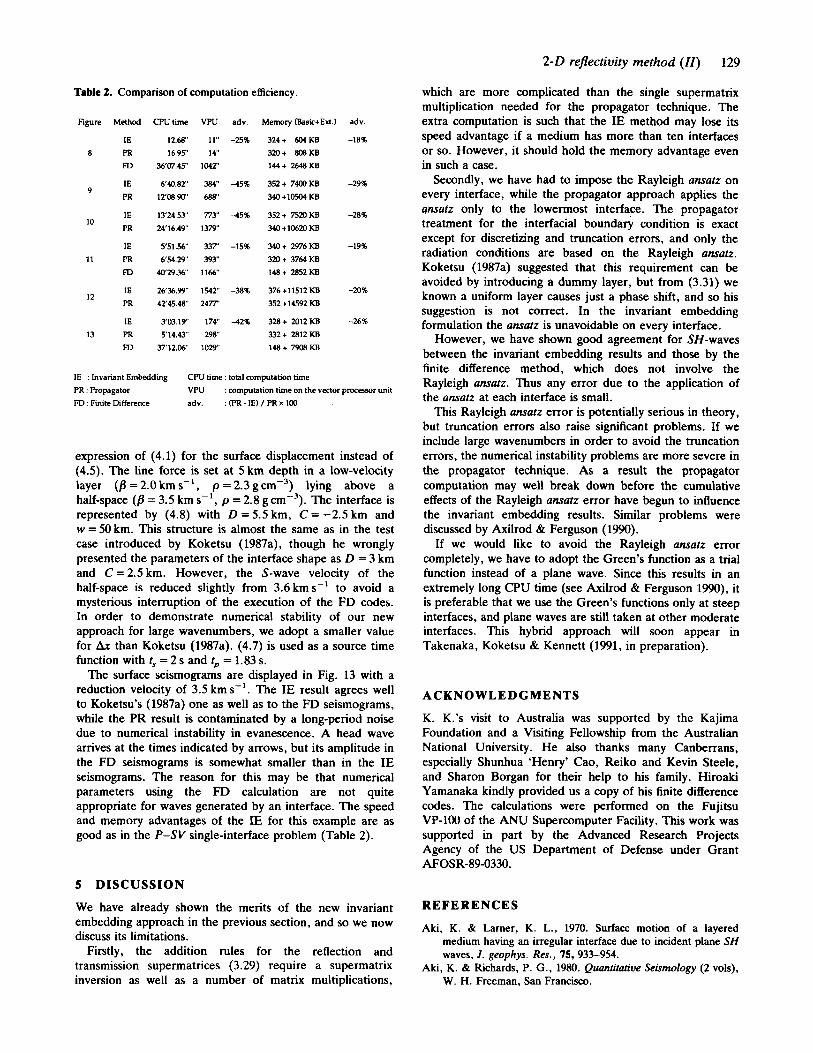
Our final example is an SH excitation problem including a transverse line force, for which we have to use the full

*----------_

__----__ 25 .----

~

0 5 10 (SeC)

Figure W. The y-component seismograms due to a line force buried in a uniform sedimentary layer at a depth of 0.5 km. The layer shown on the upper right side is bounded by a symmetric and smooth interface. All the traces are reduced with the velocity of the half-space. The arrows indicate the arrival of a head wave propagating along the interface.

2 - 0 reflectivity method (IZ) 129

which are more complicated than the single supermatrix multiplication needed for the propagator technique. The extra computation is such that the IE method may lose its speed advantage if a medium has more than ten interfaces or so. However, it should hold the memory advantage even in such a case.

Secondly, we have had to impose the Rayleigh ansatz on every interface, while the propagator approach applies the ansatz only to the lowermost interface. The propagator treatment for the interfacial boundary condition is exact except for discretizing and truncation errors, and only the radiation conditions are based on the Rayleigh ansatz. Koketsu (1987a) suggested that this requirement can be avoided by introducing a dummy layer, but from (3.31) we known a uniform layer causes just a phase shift, and so his suggestion is not correct. In the invariant embedding formulation the unsatz is unavoidable on every interface.

However, we have shown good agreement for SH-waves between the invariant embedding results and those by the finite difference method, which does not involve the Rayleigh ansatz. Thus any error due to the application of the ansatz at each interface is small.

This Rayleigh ansutz error is potentially serious in theory, but truncation errors also raise significant problems. If we include large wavenumbers in order to avoid the truncation errors, the numerical instability problems are more severe in the propagator technique. As a result the propagator computation may well break down before the cumulative effects of the Rayleigh ansatz error have begun to influence the invariant embedding results. Similar problems were discussed by Axilrod & Ferguson (1990).

If we would like to avoid the Rayleigh ansatz error completely, we have to adopt the Green’s function as a trial function instead of a plane wave. Since this results in an extremely long CPU time (see Axilrod & Ferguson 1990), it is preferable that we use the Green’s functions only at steep interfaces, and plane waves are still taken at other moderate interfaces. This hybrid approach will soon appear in Takenaka, Koketsu & Kennett (1991, in preparation).

Table 2. Comparison of computation efficiency.

Figure Method

IE 8 PR

FD

IE PR

9

IE 11 PR

m IE

j2 PR

IE 13 PR

FD

CF’Utime VPU adv.

12.68” 11” -25% 16.95 1 4

36’07.45 1042”

6‘40.82 3&2” 4 5 % 12’08.90” 688”

13’24.53 ?W 4 5 % 24‘16.49 1379”

5’51.56’ 337 -15% 6‘54.29” 3 9 3

w(y29.36” 1166“

26‘36.99- I W -38% 42‘45.40 2 4 T

3’@3.19 174 4 2 % 5’14.43 2 9 0

37’12.06’ 1029“

Memory (Basic+Ext.) adv.

324+ 604 KB -18% 320+ 808m 144+ 2648KB

352+ 7400KB -29% 340 +lo501 KB

352+ mom -2a1 340 +lo620 KB

34Q+ 2976KB -19% 320+ 3764KB 148 + 2852 KB

376 +11512 KB -20% 352 +I4592 KB

328 + 2012 KB -26% 332 + 2812 KB 1 4 8 + mKB

IE : Invariant Embedding CPU time : total computation time PR: Propagator FD : Finite Difference

VPU adv.

: computation time on the vector processor unit : (PR - IE) / PR x 100

expression of (4.1) for the surface displacement instead of (4.5). The line force is set at 5 km depth in a low-velocity layer ( f l = 2.0 km s-I, p = 2.3 g ~ m - ~ ) lying above a half-space (B = 3.5 km s-l, p = 2.8 g cm-’). The interface is represented by (4.8) with D =5.5km, C = -2.5 km and w = 50 km. This structure is almost the same as in the test case introduced by Koketsu (1987a), though he wrongly presented the parameters of the interface shape as D = 3 km and C=2.5km. However, the S-wave velocity of the half-space is reduced slightly from 3.6 kms-’ to avoid a mysterious interruption of the execution of the FD codes. In order to demonstrate numerical stability of our new approach for large wavenumbers, we adopt a smaller value for Ax than Koketsu (1987a). (4.7) is used as a source time function with ts = 2 s and tp = 1.83 s.

The surface seismograms are displayed in Fig. 13 with a reduction velocity of 3.5 km s-’. The IE result agrees well to Koketsu’s (1987a) one as well as to the FD seismograms, while the PR result is contaminated by a long-period noise due to numerical instability in evanescence. A head wave arrives at the times indicated by arrows, but its amplitude in the FD seismograms is somewhat smaller than in the IE seismograms. The reason for this may be that numerical parameters using the FD calculation are not quite appropriate for waves generated by an interface. The speed and memory advantages of the IE for this example are as good as in the P-SV single-interface problem (Table 2).

5 DISCUSSION

We have already shown the merits of the new invariant embedding approach in the previous section, and so we now discuss its limitations.

Firstly, the addition rules for the reflection and transmission supermatrices (3.29) require a supermatrix inversion as well as a number of matrix multiplications,

ACKNOWLEDGMENTS

K. K.’s visit to Australia was supported by the Kajima Foundation and a Visiting Fellowship from the Australian National University. He also thanks many Canberrans, especially Shunhua ‘Henry’ Cao, Reiko and Kevin Steele, and Sharon Borgan for their help to his family. Hiroaki Yamanaka kindly provided us a copy of his finite difference codes. The calculations were performed on the Fujitsu VP-100 of the ANU Supercomputer Facility. This work was supported in part by the Advanced Research Projects Agency of the US Department of Defense under Grant AFOSR-89-0330.

REFERENCES

Aki, K. & Lamer, K. L., 1970. Surface motion of a layered medium having an irregular interface due to incident plane SH waves, 1. geophys. Res., 75,933-954.

Aki, K. & Richards, P. G., 1980. Quantitative Seismology (2 vols), W. H. Freeman, San Francisco.

130 K. Koketsu, B. L. N . Kennett and H . Takenaka

Axilrod, H. D. & Ferguson, J. F., 1990. SH-wave scattering from a sinusoidal grating: An evaluation of four discrete wavenumber methods, Bull. seism. SOC. Am., 80, 643-655.

Bard, P.-Y. & Bouchon, M., 1980. The seismic response of sediment-filled valleys. Part 2. The case of incident P and SV waves, Bull. seism. SOC. Am., 70, 1921-1941.

Boore, D. M., Lamer, K. L. & Aki, K., 1971. Comparison of two independent methods for the solution of wave-scattering problems: Response to a sedimentary basin to vertically incident SH waves, 1. geophys. Res., 76,558-569.

Brebbia, C. A., 1978. The Boundary Element Method for Engineers, Pentech Press, London.

Campillo, M. & Bouchon, M., 1985. Synthetic SH seismograms in a laterally varying medium by the discrete wavenumber method, Geophys. 1. R. astr. SOC., 83, 307-317.

Chin, R. C. Y., Hedstrom, G. W. & Thigpen, L., 1984. Matrix methods in synthetic seismograms, Geophys. 1. R. astr. Soc.,

Dravinski, M., 1983. Scattering of plane SH waves by dipping layers of arbitrary shape, Bull. seism. SOC. Am., 73, 1303-1319.

Finlayson, B. A., 1972. The Merhod of Weighted Residuak and Variational Principles, Academic Press, New York.

Fletcher, C. A. J., 1984. Computational Galerkin Method, Springer-Verlag. New York.

Geli, L., Bard, P.-Y. & Jullien, B., 1988. The effect of topography on earthquake ground motion: A review and new results, Bull. seism. SOC. Am., 78,42-63.

Haines, A. J., 1988. Multi-source, multi-receiver synthetic seismograms for laterally heterogeneous media using F-K domain propagators, Geophys. J. Int., 95, 237-260.

Horike, M., 1988. Analysis and simulation of seismic ground motions observed by an array in a sedimentary basin, J. Phys.

77,483-502.

Earth, 36, 135-154. Kawase, H., 1988. Time-domain response of a semi-circular canyon

for incident SV, P and Rayleigh waves calculated by the discrete wavenumber boundary element method, Bull. seism. SOC. Am., 78, 1415-1437.

Kennett, B. L. N., 1972. Seismic wave scattering by obstacles on interfaces, Geophys. 1. R. mtr. Soc., 28, 249-266.

Kennett, B. L. N., 1983. Seismic Wave Propagation in Stratified Media, Cambridge University Press, Cambridge, UK.

Kennett, B. L. N., Koketsu, K. & Haines, A. J., 1990. Propagation invariants, reflection and transmission in anisotropic, laterally heterogeneous media, Geophys. J. h t . , 103, 95-101.

Koketsu, K., 1987a. 2-D reflectivity method and synthetic seismograms for irregularly layered structures-I. SH-wave generation, Geophys. J. R. astr. SOC., 89, 821-838.

Koketsu, K., 1987b. Synthetic seismograms in realistic media: a wave-theoretical approach, Bull. Earthq. Res. Inst. Tokyo, 62,

Sinchez-Sesma, F. J. & Esquivel, J. A., 1979. Ground motion on alluvial valley under the incident plane SH-waves, Bull. seism. SOC. Am., 69, 1107-1120.

Siinchez-Sesma, F. J., Herrera, I. & AvilCs, J., 1982. A boundary method for elastic wave diffraction: Application to scattering of SH waves by surface irregularities, Bull. seism. SOC. Am., 72, 473-490.

Takenaka, H., 1990. Theoretical studies on seismic wave fields in irregularly layered media, PhD thesis, Hokkaido University, Sapporo (in Japanese).

Yamanaka, H., Seo, K. & Samano, T., 1989. Effects of sedimentary layers on surface wave propagation, Bull. seism. SOC. Am., 79,631-644.

201-245.