the seismic response to overpressure: a modelling … · the seismic response to overpressure: a...

Geophysical Prospecting, 2001, 49, 523±539

The seismic response to overpressure: a modelling study based on

laboratory, well and seismic data

JoseÂ M. Carcione and Umberta Tinivella*Istituto Nazionale di Oceanografia e di Geofisica Sperimentale, Osservatorio Geofisico Sperimentale, Borgo Grotta Gigante 42C,34010 Sgonico (Trieste), Italy

Received January 2000, revision accepted March 2001

A B S T R A C T

We investigate the seismic detectability of an overpressured reservoir in the North

Sea by computing synthetic seismograms for different pore-pressure conditions. The

modelling procedure requires the construction of a geological model from seismic,

well and laboratory data. Seismic inversion and AVO techniques are used to obtain

the P-wave velocity with higher reliability than conventional velocity analysis. From

laboratory experiments, we obtain the wave velocities of the reservoir units versus

confining and pore pressures. Laboratory experiments yield an estimate of the

relationship between wave velocities and effective pressure under in situ conditions.

These measurements provide the basis for calibrating the pressure model. Over-

pressures are caused by different mechanisms. We do not consider processes such as

gas generation and diagenesis, which imply changes in phase composition, but focus

on the effects of pure pore-pressure variations. The results indicate that changes in

pore pressure can be detected with seismic methods under circumstances such as

those of moderately deep North Sea reservoirs.

I N T R O D U C T I O N

Drilling of deep gas resources is hampered by the high

risk associated with unexpected overpressure zones. Knowl-

edge of pore pressure obtained using seismic data from,

for instance, seismic-while-drilling techniques (Seisbitw,

DBSeisw, Tomexw) will help in planning the drilling process

so as to control potentially dangerous abnormal pressures.

In general, prediction of overpressure has been based on

conventional velocity analysis (e.g. Bilgeri and Ademeno

1982) and empirical models relating pore pressure to seismic

properties. Recently, Louis and Asad (1994) used a modelling

technique to analyse the amplitude variations with offset

(AVO) of pressure seals, and Pigott and Tadepalli (1996)

estimated porosities and pore pressures in clastic rocks using

AVO methods. Acoustic synthetic seismograms based on well

logs showed that a strong AVO effect is associated with steep

pressure and velocity gradients.

We study the seismic visibility of overpressure using

seismic, well and laboratory data. The analysis is intended

to provide a procedure for overpressure detection from

seismic data. We consider an area in the North Sea

sedimentary basin. This basin is 170±200 km wide and

represents a fault-bounded north-trending zone of extended

crust, flanked by the mainland of western Norway and

the Shetland Platform. The area is characterized by large

normal faults with north, northeast and northwest orien-

tations which define tilted blocks. Those flanking the

Viking Graben are shown in Fig. 1. Jurassic and older

sediments are present in the well used for this study. The

main reason for selecting this area is the fact that high

overpressure compartments were encountered during

drilling, and that even higher overpressures are expected in

future wells, down flank, towards the central Viking Graben.

The well under study is an exploration well drilled to a

total depth of 5149 mRKB (4767.4 mTVD) to test the

hydrocarbon potential of the Jurassic Brent Group, which

was encountered at about 3300 m depth. Figure 2 shows

q 2001 European Association of Geoscientists & Engineers 523

*E-mail: [email protected]

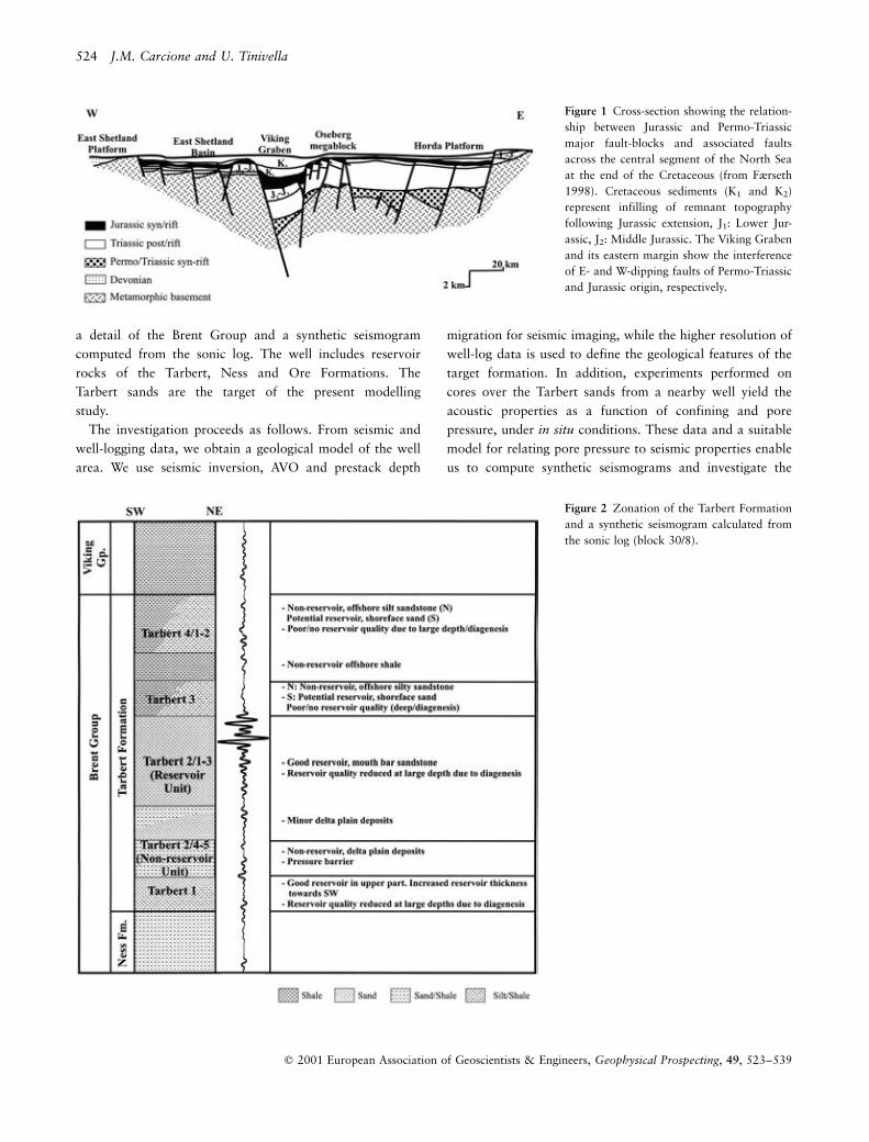
a detail of the Brent Group and a synthetic seismogram

computed from the sonic log. The well includes reservoir

rocks of the Tarbert, Ness and Ore Formations. The

Tarbert sands are the target of the present modelling

study.

The investigation proceeds as follows. From seismic and

well-logging data, we obtain a geological model of the well

area. We use seismic inversion, AVO and prestack depth

migration for seismic imaging, while the higher resolution of

well-log data is used to define the geological features of the

target formation. In addition, experiments performed on

cores over the Tarbert sands from a nearby well yield the

acoustic properties as a function of confining and pore

pressure, under in situ conditions. These data and a suitable

model for relating pore pressure to seismic properties enable

us to compute synthetic seismograms and investigate the

Figure 1 Cross-section showing the relation-

ship between Jurassic and Permo-Triassic

major fault-blocks and associated faults

across the central segment of the North Sea

at the end of the Cretaceous (from Fñrseth

1998). Cretaceous sediments (K1 and K2)

represent infilling of remnant topography

following Jurassic extension, J1: Lower Jur-

assic, J2: Middle Jurassic. The Viking Graben

and its eastern margin show the interference

of E- and W-dipping faults of Permo-Triassic

and Jurassic origin, respectively.

Figure 2 Zonation of the Tarbert Formation

and a synthetic seismogram calculated from

the sonic log (block 30/8).

524 J.M. Carcione and U. Tinivella

q 2001 European Association of Geoscientists & Engineers, Geophysical Prospecting, 49, 523±539

seismic visibility of overpressure. This work is part of the

modelling work-package for the European Union project

`Detection of overpressure zones with seismic and well data'

(ODS), and as such, we make use of data provided by the

different partners.

T H E G E O L O G I C A L M O D E L

The location of the 2D seismic line SH9502-402, crossing

well 30/8-1S, is approximately 165 km west of Bergen

(Norway). The data were acquired using a 6 km streamer

length, with a shot spacing of 25 m, a trace interval of 12.5 m

and a sampling rate of 2 ms. The standard processing

sequence applied to the data includes common-depth-point

sorting, correction for geometrical spreading, low-cut filter-

ing (to remove low-frequency noise), trace muting, and

suppression of multiples. We consider a maximum offset of

3.2 km, since larger offsets present a very low signal-to-noise

ratio. This represents a maximum angle of incidence of about

258 at the target level. The conventional stacked section, with

a multiplicity of 60, is shown in Fig. 3.

The first version of the P-wave velocity model is obtained

from the stacking velocities (Fig. 4, model 1). This model has

relatively low resolution and is not suitable for seismic

modelling analysis. A detailed interpretation of the existing

3D seismic data set in the study area, performed by one of the

partners of the ODS project, provides a suitable geological

model. Cretaceous and younger sequences are largely

unfaulted and do not require additional interpretation,

other than the usual standard procedure. The geological

modelling procedure for the structurally more complex

Jurassic sequences involved the generation of a seismic-

coherence volume to define the main reservoir units and the

associated minor faulting. The model is shown in Fig. 5

(model 2). A detailed interpretation of the target area (Fig. 6)

Figure 3 Stacked time-section for line SH9502-402.

Figure 4 Geological model obtained from a conventional velocity

analysis of seismic line SH9502-402 (model 1).

Seismic response to overpressure 525


is performed by including well-logging information (sonic

and density logs, Fig. 7). The main geological structures are: a

shallow low-velocity unit below the sea-floor (1), the Utsira

Formation (2), a diapiric sequence (Hordaland Group) (3),

the Balder Formation (4), the Cretaceous formations (5), the

Viking Group (6) and the Brent Group, i.e. the Jurassic

reservoir (7) and the Ness Formation (8). The Jurassic

sequence includes four main units of the Tarbert Formation:

Tarbert-4, Tarbert-3 (the top of the Brent Formation),

Tarbert-2 (the reservoir) and Tarbert-1. On the basis of

well-logging data, we include a high-velocity layer above the

base of the Cretaceous (HVL), two layers in Tarbert-4 and

four layers in the reservoir sands, three of which are very thin

compared with the seismic wavelength (Kallweit and Wood

1982). In this case, Backus averaging (Backus 1962) is

used to obtain the velocity field at the levels of seismic

resolution. No lateral velocity variations are assumed in

this interpretation.

In order to obtain a model with lateral velocity variations,

we use the seismic inversion algorithm of the GeoDepthq

software package (Paradigm Geophysical). Firstly, we inter-

pret the stacked section by picking the main reflectors (see

Fig. 3). These are the sea-floor (A), a shallow event (B), the

top of the Utsira Formation (C), the top of the diapiric

sequence (D), the top of the Balder Formation (E), the base

and top of the Cretaceous (F), and three events in the Jurassic

sequence (G, H and I). On the basis of these picks, the

algorithm identifies the events in the prestack domain using

coherence analysis. The velocity analysis provides the initial

model for the inversion algorithm. This uses ray tracing to

compute the moveout curves, and we choose the maximum

semblance between data and predictions. This process is

performed within a time window around the common

midpoints (CMPs) predicted by the ray-tracing algorithm.

Next, a depth section is generated using the interval velocities

obtained with the inversion technique. Finally, the model is

refined by using the horizon-based global-depth tomography

algorithm, using depth delays. These delays give information

about the residual error in moveout after prestack migration

is applied to the data. This information is used to flatten the

gathers. The degree of non-flatness yields a qualitative

estimation of the error in the determination of the model.

The tomographic algorithm uses these non-flatness estimates

and finds an updated model with minimum error. The input

to this process is the above-mentioned depth model and the

conventional depth model obtained from velocity analysis.

The final updated model obtained with the GeoDepthq

package is shown in Fig. 8 (model 3). The main differences

compared with the model shown in Fig. 5 are the presence of

lateral velocity variations and the lack of the detailed features

Figure 5 Geological model obtained from 3D seismic data and a

priori geological information around well 30/8-1S. The modelling

procedure involved the generation of a seismic-coherence volume to

define the main reservoir units and the incorporation of fault-data of

the study area (model 2).

Figure 6 Interpretation of the reservoir units, using seismic,

geological and well-logging (sonic- and density-log) information.



of the Brent Group. Figure 9 shows the P-wave velocity

profile at the well location, corresponding to model 1 (dotted

line), model 2 (thick broken line) and model 3 (thin broken

line). The velocities obtained with conventional velocity

analysis agree with the log velocities at shallow depths but

differ for deep layers (Stewart, Huddleston and Tan 1984).

In order to test the velocity models we perform 2D prestack

depth migration for each model, using the Seismic Unix

software (a public-domain package available from Colorado

School of Mines). The migrated sections are shown in Figs

10(a) (model 1), 10(b) (model 2) and 10(c) (model 3). Figure

10(d) shows a detail of the interpretation around the target

formation. Model 1 is not suitable for obtaining good

imaging of the structures. Model 3 is the best (mainly in

the target zone, between 3.1 and 3.7 km depth) since lateral

velocity variations are taken into account. The events

indicated with dots in Fig. 10(d) are multiples. The broken

lines correspond to reflections and the continuous lines to the

main fault near the well. These events cannot be appreciated

in the stacked unmigrated section (Fig. 3).

Table 1 shows the elastic properties which result from the

interpretation and well-log information. The shear-wave

velocity for layers 2±8 is given by

V S�m=s� � 2792� 0:765 V P�m=s�; �1�

where VP is the P-wave velocity. This empirical equation is

obtained by integrating the information from nearby wells,

where logging measurements of shear-wave velocity were

available. This relationship holds for brine-filled clastic

rocks. The other properties are the density r, the P-wave

and S-wave acoustic impedances IP and IS, respectively, and

Poisson's ratio s .

Amplitude variations with offset (AVO) analysis

AVO analysis is performed to obtain more information about

the elastic properties, in particular about the shear-wave

velocity of the target formation. We use two approaches: (i)

the GeoDepthq algorithm and (ii) a least-squares algorithm.

Figure 11(a) shows a CMP gather at the well location. The

top of the reservoir is indicated by an arrow in Fig. 3. This

event corresponds to the interface Tarbert-3/Tarbert-2 (see

Table 1). The AVO trend is shown in Fig. 11(b), where the

open circles mark relative minimum amplitudes of the event

picked in the time domain and the continuous line is the best-

fit curve. We consider the minimum of the event, because

there is a velocity inversion at the interface. The GeoDepthq

algorithm, based on the linearization of Zoeppritz's equa-

tions, requires the following processing sequence: geome-

trical-spreading correction, surface-consistent scaling,

correction for source and receiver directivities, correction

for source and receiver array patterns, and attenuation

compensation. We assume an average quality factor of 150

in view of the nature of the formations (SchoÈn 1996). After

applying this model-based conditioning to the data, we

analyse the variations in the amplitude versus angle of

incidence and obtain additional sections for various elastic

parameters (P- and S-wave velocity and impedance reflectiv-

ities, fluid factor, etc.). The relationship between offset x and

angle of incidence u is calculated using the approximation

x � sin�u�V 2rmst�x�

V P;

where VP is the vertical P-wave velocity of the upper layer,

Vrms is the root-mean-square velocity and t(x) is the time

at offset x (Walden 1991). The analysis indicates that

Figure 7 Sonic and density logs in well 30/8-

1S. The S-wave log is obtained from the P-

wave log by using the empirical relationship

(1).



the impedance reflectivities are more negative than the

velocity reflectivities at the Tarbert-2 units (P-wave impe-

dance reflectivity <20.077, P-wave velocity reflectivity

<20.037), in agreement with the well-log data (see Fig. 7

and Table 1).

The second AVO algorithm can be summarized as follows:

(i) selection and picking of reflectors in the CMP gather,

(ii) frequency and velocity analysis, (iii) extraction of

amplitudes versus offset and (iv) a least-squares inversion to

obtain the acoustic properties by fitting the data to the exact

theoretical reflection coefficient. We identify the top of the

reservoir (Fig. 3) and pick the events in the CMP gather (Fig.

11). A frequency analysis gives a dominant frequency of

25 Hz. After applying geometrical spreading, attenuation

(quality factor equal to 150) and overburden corrections, we

obtain the normalized reflection coefficients. They are

normalized with respect to the zero-offset reflection coeffi-

cient computed from the well-log data. We assume an

isotropic and viscoelastic rheological equation, for which it

is necessary to determine six acoustic properties: the P-wave

velocity VP, the shear-wave velocity VS and the density r,

for both the lower and upper media. We then minimize, in a

least-squares sense, the difference between the reflection

coefficient obtained from the seismic data and the

theoretical reflection coefficient (Carcione 1997). We assume

P-wave (S-wave) quality factors of 150 (100) and 30 (20) for

the upper and lower layers (SchoÈn 1996), respectively (in fact,

attenuation has a limited influence on the offsets under

consideration (Carcione, Helle and Zhao 1998)). Table 2

shows the best fit of the reflectivities using approach

(ii), compared with those obtained from the well data,

where VS is given by equation (1) without taking the presence

of gas into account (see also Fig. 7). The values are negative

since the wave velocities and density of Tarbert-3 are greater

than the wave velocities of Tarbert-2 (see Table 1). The

main difference is in the shear-wave velocity, which we

attribute to the presence of gas in Tarbert-2/1. The original

Poisson's ratio of the Tarbert-2/1 to Tarbert-2/3 units is

approximately 0.29. The AVO analysis implies a Poisson's

ratio of 0.25, which is consistent with the presence of gas

in the pore space (Khazanehdari, McCann and Sothcott

1998, paper presented at Conference on Pressure Regimes

in Sedimentary Basins and their Prediction, Del Lago resort,

Lake Conroe, Texas, USA). Therefore, the shear-wave

velocity for the Tarbert-2 units is calculated using a Poisson's

ratio of 0.25.Figure 8 Geological velocity model obtained from the interpretation

of seismic line SH9502-402 with the GeoDepthq software package

(model 3).

Figure 9 P-wave velocity profiles at the well location, corresponding

to models 1, 2 and 3.



P R E S S U R E M O D E L

First, we introduce some useful definitions of the different

pressures considered in this work. Pore pressure, also known

as formation pressure, is the in situ pressure of the fluids in

the pores. The pore pressure is equal to the hydrostatic

pressure when the pore fluids only support the weight of the

overlying pore fluids (mainly brine). The lithostatic or

confining pressure is due to the weight of overlying

sediments, including the pore fluids. In the absence of any

state of stress in the rock, the pore pressure attains lithostatic

pressure and the fluids support all the weight. However,

fractures perpendicular to the minimum compressive stress

direction appear for a given pore pressure, typically 70±90%

of the confining pressure. In this case, the fluid escapes from

the pores and pore pressure decreases. A rock is said to be

overpressured when its pore pressure is significantly greater

than the hydrostatic pressure. The difference between pore

pressure and hydrostatic pressure is called differential

pressure. Acoustic and transport properties of rocks generally

depend on effective pressure, a linear combination of pore

and confining pressures (see equation (2)). Various physical

processes cause anomalous pressures on an underground

fluid. The most common causes of overpressure are thermal

expansion of water, compaction disequilibrium and cracking,

i.e. oil-to-gas conversion (Mann and Mackenzie 1990; Luo

and Vasseur 1994).

In the following analysis we compute the variations in pore

and fluid volume, which allow the calculation of the rock

porosity and saturations as a function of pore pressure, the

independent variable. These variations take place at nearly

constant confining pressure (i.e. constant depth) and tem-

perature. The changes are due solely to the compressibility

effect, since at nearly constant temperature, thermal effects

can be neglected. The reference state, for which all the

properties are known, is the hydrostatic state. We consider

constant composition within each phase, since the aim is to

study variations due to pure pore-pressure effects rather than

changes due to variations in material composition. A pressure

model for variable composition was given by Berg and Gangi

(1999), who calculated the excess pore pressure as a function

of the fraction of kerogen converted to oil and the fraction of

oil converted to gas. This model can easily be incorporated

into the present theory.

We assume a closed rock unit at a fixed depth z and

temperature T, representing a pressure compartment, which

is characterized by an effective seal that prevents pressure

equilibration to normal hydrostatic pressure (Bradley and

Powley 1994). The lithostatic pressure for an average

sediment density rÅ is equal to pc � �rgz; where g is the

Table 1 Material properties of the North Sea model

dbsf VP VS r IP IS

Layer Medium (m) (m/s) (m/s) (kg/m3) (kg/m2s) (kg/m2s) s

0 Sea-water 0 1464 0 1040 1.464 0 0.5

1 Shallow layer 534 1890 750 1800 3.402 1.350 0.41

2 Utsira Formation 786 2030 762 1800 3.654 1.372 0.42

3 Diapiric sequence 1978 2121 832 2027 4.300 1.686 0.41

4 Balder Formation 2328 2582 1185 2271 5.864 2.691 0.37

5 Cretaceous 2945 3206 1662 2511 8.050 4.173 0.32

HVL Cretaceous 3036 4253 2457 2626 11.168 6.452 0.25

6 Viking Group 3230 3266 1699 2528 8.256 4.295 0.31

7 Tarbert-4/1 3273 3894 2184 2595 10.105 5.667 0.27

7 Tarbert-4/2 3295 3472 1862 2601 9.031 4.843 0.30

7 Tarbert-3 3324 3876 2171 2558 9.915 5.553 0.27

7 Tarbert-2/1 3380 3601 1960 2362 8.506 4.629 0.29

7 Tarbert-2/2 3391 3816 2117 2502 9.548 5.297 0.28

7 Tarbert-2/3 3420 3623 1954 2416 8.753 4.721 0.29

7 Tarbert-2/4 3438 4140 2375 2640 10.930 6.275 0.25

7 Tarbert-2/5 3450 3965 2210 2457 9.742 5.430 0.27

7 Tarbert-1 3480 4124 2365 2534 10.450 5.993 0.25

8 Ness Formation Ð 4101 2083 2538 10.408 5.287 0.32

dbsf, depth of base of group/formation/member below the sea-floor.



acceleration of gravity. On the other hand, the normal

hydrostatic pore pressure is approximately pH � rwgz; where

rw is the density of brine.

In general, seismic properties, such as wave velocity and

attenuation, depend on effective pressure,

pe � pc 2 np; �2�

where pe, pc and p are the effective, confining and pore

pressures and n # 1 is the effective stress coefficient. Note

that the effective pressure equals the confining pressure at

zero pore pressure. It is found that n < 1 for static measure-

ments of the compressibilities (Zimmerman, Somerton and

King 1986), while n is approximately linearly dependent

on the differential pressure pd � pc 2 p for dynamic experi-

ments (Gangi and Carlson 1996; Prasad and Manghnani

1997): n � n0 2 n1pd; where n0 and n1 are constant

coefficients. Using this equation, the effective pressure (2)

can be written as

pe � pc 2 �n0 2 n1pc�p 2 n1p2: �3�

We know the porosity and fluid saturations at the

hydrostatic pressure, and want to compute these quantities

at a pore pressure higher than the hydrostatic pressure.

Assuming oil, gas and brine in the pore space, the volume

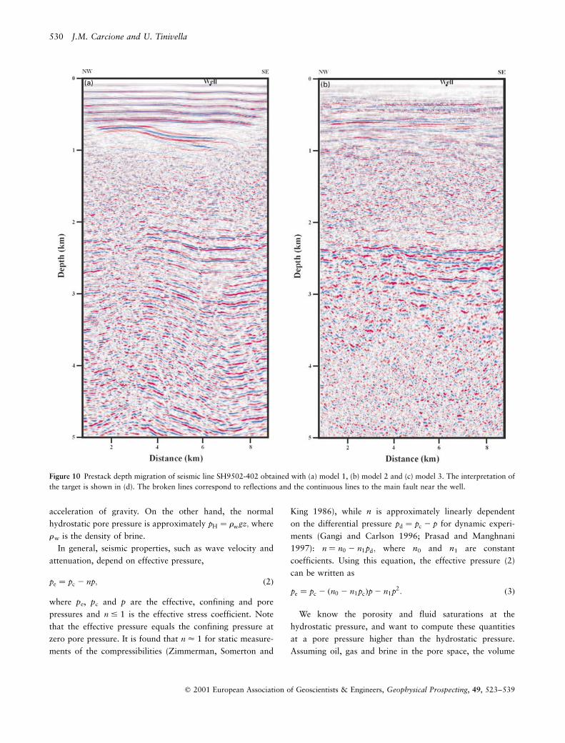
Figure 10 Prestack depth migration of seismic line SH9502-402 obtained with (a) model 1, (b) model 2 and (c) model 3. The interpretation of

the target is shown in (d). The broken lines correspond to reflections and the continuous lines to the main fault near the well.



balance is vpore � vo � vg � vw; where vpore is the pore

volume, and vo, vg and vw are the volumes of oil, gas and

brine in the pore space, respectively. Since no mass (of the

organics or the brine) leaves the pore space and the depth

remains constant, the volume changes do not depend on mass

and temperature, and we have

dvpore � 2vpore

2pe

� �dpe � 2vo

2p� 2vg

2p� 2vw

2p

� �dpe; �4�

with

cp � 21

vpore

dvpore

dpe

; co � 21

vo

dvo

dp; cg � 2

1

vg

dvg

dp;

cw � 21

vw

dvw

dp; �5�

as the compressibilities for the pore space, oil, gas and brine.

Note that the pore `senses' the effective pressure, but the fluid

`senses' the pore pressure.

We assume that the compressibilities of the oil and brine

are independent of pressure (it can be shown that the

variations are less than 10% in the range of pore pressures

investigated here (Batzle and Wang 1992)), and those of

the gas and the rock depend on pressure. Moreover, we

consider the following functional form for cp as a function of

Figure 10 Continued



effective pressure:

cp � c1p � ape � b exp�2pe=p*�; �6�

where c1p ; a , b and p* are coefficients obtained by fitting the

experimental data. Similar functional forms (6) are used to fit

experimental data of pore compressibility (Zimmerman et al.

1986; Prasad and Manghnani 1997).

Integration of equations (5) from the hydrostatic pressure

pi � pH to a given pore pressure p yields

vpore�p� � vpore;i exp�E�Dp��; �7�

vo�p� � voi exp�2coDp�; �8�

vg�p� � vgi exp 2cg

�p

pi

cg�p� dp

� ��9�

and

vw�p� � vwi exp�2cwDp�; �10�

Figure 11 (a) CMP gather at the well

location and (b) AVO trend of the top of

the reservoir. The open circles indicate the

reflection from the top of the reservoir (Brent

Formation) and the open circles in (b)

indicate the relative minimum amplitudes of

the event picked in the time domain.

Table 2 Reflectivity at the top of the reservoir

DVP/VP DVS/VS Dr /r

Well data 20.0709 20.0976 20.0766

AVO analysis 20.0708 20.0451 20.0793



where Dp � p 2 pH;

E�Dp� � 2c1p Dpe � 1

2a�p2

e 2 p2ei� � bp*�exp�2pe=p*�

2 exp�2pei=p*��;and Dpe � pe 2 pei; the index i denotes the initial (hydro-

static) state and pei is the effective pressure at the initial

state.

Using equations (7), (8)±(10), and since the initial

saturations are

Swi � vwi=vpore;i; Soi � voi=vpore;i; Sgi � vgi=vpore;i; �11�the pore-volume balance equation becomes

exp�E�Dp�� Swi exp�2cwDp� � Soi exp�2coDp�

� Sgi exp 2cg

�p

pi

cg�p� dp

� �: �12�

As the pore pressure changes from pi to p, the pore

volume changes from vpore,i to vpore,i exp[E(Dp)]. The

saturations are equal to the corresponding volumes

divided by the pore volume. Using equations (8) and (10),

the requirement that Sgi � 1 2 Swi 2 Soi gives for the oil,

brine and gas saturations,

So � Soi exp�2coDp 2 E�Dp��; �13�Sw � Swi exp�2cwDp 2 E�Dp�� 14�and

Sg � 1 2 Sw 2 So; �15�respectively. On the other hand, the fluid proportions are

fo � fSo; fw � fSw; fg � fSg; �16�where f � vpore=�vpore � vs� is the total porosity, with vs

denoting the volume of the solid part. This can be calculated

Figure 12 Regression fits to (a) dry-rock moduli Km and mm and (b)

pore compressibility cp.Figure 13 Compressional-wave velocity as a function of pore

pressure for (a) full brine saturation and (b) partial saturation. In

this case, the initial gas and brine saturations are Sgi � 0:85 and

Swi � 0:15; respectively. The confining pressure is 71.06 MPa. The

dry-rock velocities are shown as broken lines. In this case, the

horizontal axis corresponds to the confining pressure with zero pore

pressure.



from the initial porosity f i (at hydrostatic pressure), since

fi � vpore;i=�vpore;i � vs�: Thus, vs � vpore;i�1=fi 2 1� and

using (7), we obtain

f � fi exp�E�Dp��1 2 fi{1 2 exp�E�Dp��} ; �17�

assuming incompressible grains in this calculation �vs <constant�: Defining f s as the mineral matrix fraction, we

have fs � 1 2 f: The pressure model can be refined by

assuming the dependence on pressure and temperature of oil

and brine compressibilities, and the influence of sodium

chloride on brine properties. If one considers, for instance,

the empirical formulae published by Batzle and Wang (1992),

the solution can be obtained by numerical integration of the

compressibilities.

Seismic velocities

The isothermal gas bulk modulus Kg and the gas compres-

sibility cg � K21g depend on pressure. The latter can be

calculated from the van der Waals equation,

�p� ar2g��1 2 brg� � rgRT ; �18�

where p is the gas pressure, rg is the gas density, T is the

absolute temperature and R is the gas constant. Moreover, a

good approximation can be obtained using a �0:225 Pa �m3=mole�2 � 879:9 MPa �cm3=g�2 and b � 4:28 �1025 m3=mole � 2:675 cm3=g (one mole of methane, CH4,

corresponds to 16 g). Then,

cg � 1

rg

drg

dp� rgRT

�1 2 brg�22 2ar2

g

" #21

: �19�

In sandstones, the pore compressibility cp is closely related

to the bulk modulus of the matrix Km (the compressibility cp

is denoted by Cpp by Zimmerman et al. (1986) and by K21fp by

Mavko and Mukerji (1995), and Km corresponds to C21bc and

K21dry; respectively). Using the present notation, cp can be

expressed approximately as

cp � 1

Km2

1

K s

� �1

f2

1

K s; �20�

where f depends on the pore-pressure difference Dp at

constant confining pressure. Since dry-rock wave velocities

are practically frequency-independent, the seismic bulk

moduli Km and mm versus confining pressure can be obtained

from laboratory measurements in dry samples. If VP0 and VS0

are the experimental dry-rock compressional- and shear-wave

velocities, the moduli are given approximately by

Km � �1 2 f�rs V 2P0 2

4

3V 2

S0

� �; mm � �1 2 f�rsV

2S0;

�21�where r s is the grain density and f is the porosity. We recall

that Km is the rock modulus at constant pore pressure, i.e. the

case when the bulk modulus of the pore fluid is negligible

compared with the frame bulk modulus, as, for example, air

at room conditions (Mavko and Mukerji 1995).

The seismic velocities of the overpressured porous rock are

Table 3 Material properties for Tarbert-2 sandstone at 3.4 km depth

and hydrostatic pore pressure

Grain r s � 2650 kg/m3

Ks � 37 GPa

m s � 39 GPa

Fluids rg � 157 kg/m3

Kg � 92.6 MPa

hg � 0.02 � 1023 Pa s

rw � 1045 kg/m3

Kw � 2.25 GPa

hw � 1.8 � 1023 Pa s

Matrix Km � 17.95 GPa

mm � 8.77 GPa

f � 0.189

k � 10212 m2

T � 2

Table 4 Material properties of the reservoir units

VP(Log) VP(Lab) VS(Log) VS(AVO) VS(Lab) r(Log) r (Lab)

Medium (m/s) (m/s) (m/s) (m/s) (m/s) (kg/m3) (kg/m3)

Tarbert-2/1 3601 3517 1960 2079 2045 2362 2202

Tarbert-2/2 3816 3517 2117 2203 2045 2502 2202

Tarbert-2/3 3623 3517 1954 2092 2045 2416 2202

AVO, from amplitude versus offset analysis (53 MPa); Lab, from laboratory experiments (53 MPa); Log, from well-log data (33.55 MPa).



computed using Biot's theory of dynamic poroelasticity (Biot

1962; Carcione 1998), where fluid saturations and porosity

versus pore pressure are given by equations (13), (14), (15)

and (17). The velocities are given by (see Appendix)

V P^ � Re1

V *P^

!" #21

; V S � Re1

V *S

!" #21

; �22�

where V *P^ are the complex velocities of the fast (+) and slow

(2) waves, V *S is the complex shear-wave velocity and Re

denotes the real part.

S Y N T H E T I C S E I S M O G R A M S F O R

D I F F E R E N T P R E S S U R E C O N D I T I O N S

Seismic properties of the reservoir sandstone versus pore

pressure

The Tarbert-2 sandstone is located at a depth z � 3:38 km

below the sea-floor (the water depth is approximately

100 m). From density-log data, the average sediment density

from the surface to the Tarbert-2 sandstone is r��2118 kg=m3; which gives a confining pressure of pc �71:06 MPa: The hydrostatic pressure is pH � 33:55 MPa

(assuming rw � 1040 kg=m3�: The well report indicates a

temperature between 1108C and 1208C, which is consistent

with a surface temperature T0 � 108C and a geothermal

gradient G � 308C=km (on the basis of the linear relationship

T � T0 �Gz�: The pore pressure measured in the well is

53 MPa (530 bar).

The laboratory data are provided by the Institute of

Sedimentology at Reading University. On the basis of these

data and equations (21) for pc ranging from 0 to 72 MPa,

best-fit estimates of the dry-rock moduli versus confining

pressure are

Km�GPa� � 17:87� 0:011pc�MPa�2 10:15 exp�2pc�MPa�=16:51�

and

mm�GPa� � 7:58� 0:023pc�MPa�2 7:64 exp�2pc�MPa�=7:77�;

and cp in MPa is given by equation (6), with c1p � 0:1483;

a � 20:0005; b � 0:3237; p* � 9:56: The pore compressi-

bility cp is obtained from equation (20) by assuming that the

porosity is that at hydrostatic pore pressure (this approxima-

tion is supported by experimental data obtained by Dome-

nico (1977) and Han, Nur and Morgan (1986)). The best-fit

plots for Km and mm (a) and cp (b) versus pore pressure are

illustrated in Fig. 12.

In order to obtain the moduli for different combinations of

the confining and pore pressures we make the substitution

pc ! pe � pc 2 np; where we assume, following Gangi and

Carlson (1996), that n depends on differential pressure and is

given by

n � n0 2 n1pd:

This relationship of n versus differential pressure is in good

agreement with the experimental values corresponding to the

compressional-wave velocity obtained by Christensen and

Wang (1985) and Prasad and Manghnani (1997). Experi-

mental evidence indicates that n is different for each physical

property. A linear best-fit of the values provided by Reading

University yields

bulk modulus and compressibility : n0 � 1;

Figure 14 Synthetic RVSP (vertical compo-

nent of the particle velocity) obtained with

model 2 and a pore pressure of 53 MPa. The

source (drill-bit) is located in the well at 3 km

depth and the receivers are deployed at the

sea-bottom (ocean-bottom cable). The bit is

approximately 330 m above the top of the

Brent Formation.



n1 � 0:01 MPa21

and

shear modulus : n0 � 1; n1 � 0:012 MPa21:

Table 3 indicates the properties for the Tarbert-2 sandstone.

The gas properties, according to the petrophysical report of

the well, correspond to a pressure of 53 MPa. They give a

sound velocity of 768 m/s. The matrix properties correspond

to those at the initial (hydrostatic) pore pressure. The brine

density and bulk modulus are assumed to be pressure-

independent.

Figure 13(a) shows the compressional-wave velocity versus

pore pressure for a confining pressure pc � 71:06 MPa

(continuous lines), compared with the experimental values

provided by Reading University for full brine saturation

�Swi � 1:�: They also provided the velocities for different

confining and pore pressures. Knowing n, it is possible to

obtain the velocities for different combinations of the pore

and confining pressures, in particular for pc � 71:06 MPa and

variable pore pressure. Each experimental point in Fig. 13(a)

corresponds to a pore pressure p, that is a solution of the

second-degree equation (3). The velocity decreases substan-

tially with increasing pore pressure, mainly because of the

opening of compliant cracks. This information is contained in

the behaviour of the dry-rock moduli as a function of

confining pressure.

In the following, we assume an initial gas saturation Sgi �0:85 and brine saturation Swi � 0:15; which are those given

in the well report. Figure 13(b) shows the wave velocities

versus pore pressure at a confining pressure of 71.06 MPa.

The dry-rock velocities are shown as broken lines (in this

case, the horizontal axis corresponds to the confining

pressure with zero pore pressure). Because of the decrease

in density, the S-wave velocity is higher than the S-wave

velocity for full brine saturation (see Fig. 13a). The small

difference between the dry-rock and wet-rock velocities in

Fig. 13(b) indicates that in this case the presence of gas has

not had a major effect on the velocities.

The properties of the reservoir layers obtained from

seismic, well-log and laboratory data (one sample) are given

in Table 4 for a pore pressure of 53 MPa, which was the

pressure regime when the seismic data were acquired

(although the well-log velocities should correspond, in

principle, to the hydrostatic pressure 33.55 MPa because

they are obtained from open-hole measurements). Since in

this study we have both well and laboratory data, we assume

that the properties of the reservoir are those obtained with

laboratory data, as indicated in Table 4. The wave velocities

Figure 15 Difference between the 53 MPa

and hydrostatic-pressure synthetic seismo-

grams. The main reflection corresponds to

the top of the reservoir.

Figure 16 AVO trends of the first event in the difference seismo-

grams, corresponding to different pore-pressure regimes. The

continuous lines are best-fit regression curves.



of the dry rock, determined by laboratory measurements, give

estimates of the pore compressibility and bulk moduli in the

low-frequency (relaxed) regime. Since dissipation mechan-

isms are caused mainly by grain/fluid interactions, dry-rock

velocities are approximately frequency-independent (Spencer

1981).

Synthetic seismograms

We compute 2D synthetic seismograms with the source

located in the well at 3 km depth (see Fig. 6) and the receivers

deployed at the sea-bottom (ocean-bottom cable (OBC)). The

numerical experiment simulates a reverse vertical seismic

profile (RVSP), using the drill-bit as a source. Note that to

obtain real-data RVSP requires an autocorrelation of the

drill-bit data with the pilot signal travelling through the drill-

string (Aleotti et al. 1999). The synthetic seismograms are

computed with a modelling algorithm based on the velocity±

stress formulation of the isotropic-viscoelastic wave equation.

The Fourier pseudospectral method is used to calculate the

spatial derivatives and a fourth-order Runge-Kutta technique

is used to obtain the wavefield recursively in time (Carcione

1992). The numerical mesh has 231 � 231 points with a grid

spacing DX � DZ � 20 m: The source is a Ricker-type

wavelet with a dominant frequency of 25 Hz. We assume

P-wave (S-wave) quality factors of 150 (100) for all the

layers. Five synthetic seismograms have been computed,

corresponding to different pore-pressure regimes in the

reservoir: 33.55 MPa (hydrostatic pressure), 40 MPa,

53 MPa, 65 MPa and 70 MPa. The synthetic seismogram

for a pore pressure of 53 MPa (measured pressure while

drilling) is shown in Fig. 14. The first strong event is

the direct wave, which masks the reflected event from the

base of the Cretaceous. The reflection from the top of

the reservoir is located between 1.6 s and 1.75 s. Figure 15

shows the difference between the 53 MPa and hydrostatic-

pressure seismograms. Similar difference seismograms

have been obtained for 40, 65 and 70 MPa. The AVO trends

of the first event in these difference seismograms are

shown in Fig. 16, where the continuous lines are best-fit

regression curves. The behaviour is similar to that shown

in Fig. 11(b), obtained from the real-data CMP gather.

Strong and negative differential AVO effects are associated

with high pore pressures, approaching the confining pressure.

These effects are more important for near and medium

offsets.

C O N C L U S I O N S

Seismic data and a suitable rock-acoustics model, relating the

seismic properties to pore pressure, enable the determination

of overpressure in advance of drilling. This modelling study

shows the influence of high pore pressures on seismic

velocities and amplitude variations with offset. The model

relating pore pressure to seismic velocity requires calibration

with laboratory measurements of wave velocities versus

confining and pore pressures. Measurements of dry-rock

moduli and pore compressibility versus confining pressure are

essential for proper use of the Biot±Gassmann equations,

since these moduli contain implicit microstructural informa-

tion. In addition, experiments on saturated samples for

different confining and pore pressures give the effective-stress

coefficient, which enables the calculation of seismic proper-

ties versus effective pressure. On the other hand, seismic

inversion and AVO techniques can be used to obtain wave

velocities with higher reliability than conventional processing

techniques, and well-log data are essential in order to provide

a high-resolution geological model, appropriate for over-

pressure modelling studies. In the particular case of the North

Sea reservoir investigated, strong and negative differential

AVO effects are associated with overpressure. The effects are

important at high pore pressures and near and medium

offsets.

A C K N O W L E D G E M E N T S

This work was supported by the European Union under

the project `Detection of overpressure zones with seismic

and well data'. We thank our partners of the ODS

project, Hans B. Helle, Clive McCann, John J. Walsh and

Bill Martin, for their co-operation in making the data

available. We are grateful to Zvi Koren and Dan Kosloff

of Paradigm Geophysical for providing the GeoDepthq

software.

R E F E R E N C E S

Aleotti L., Poletto F., Miranda F., Corubolo P., Abramo F. and

Craglietto A. 1999. Seismic while-drilling technology: use and

analysis of the drill-bit seismic source in cross-hole survey.

Geophysical Prospecting 47, 25±39.

Backus G.E. 1962. Long-wave elastic anisotropy produced by

horizontal layering. Journal of Geophysical Research 67, 4427±

4440.

Batzle M. and Wang Z. 1992. Seismic properties of pore fluids.

Geophysics 57, 1396±1408.

Berg R.R. and Gangi A.F. 1999. Primary migration by oil-generation



microfracturing in low-permeability source rocks. Application to

the Austin chalk, Texas. AAPG Bulletin 83, 727±756.

Berryman J.G., Thigpen L. and Chin R.C.Y. 1988. Bulk elastic wave

propagation in partially saturated porous solids. Journal of the

Acoustical Society of America 84, 360±373.

Bilgeri D. and Ademeno E.B. 1982. Predicting abnormally pressured

sedimentary rocks. Geophysical Prospecting 30, 608±621.

Biot M.A. 1962. Mechanics of deformation and acoustic propagation

in porous media. Journal of Applied Physics 33, 1482±1498.

Bradley J.S. and Powley D.E. 1994. Pressure compartments in

sedimentary basins: a review. AAPG Memoir 61, 3±26.

Carcione J.M. 1992. Modeling anelastic singular surface waves in the

Earth. Geophysics 57, 781±792.

Carcione J.M. 1997. Reflection and refraction of qP-qS plane shear

waves at a plane boundary between viscoelastic transversely

isotropic media. Geophysical Journal International 129, 669±680.

Carcione J.M. 1998. Viscoelastic effective rheologies for modelling

wave propagation in porous media. Geophysical Prospecting 46,

249±270.

Carcione J.M., Helle H. and Zhao T. 1998. The effects of attenuation

and anisotropy on reflection amplitude versus offset. Geophysics

63, 1652±1658.

Christensen N.I. and Wang H.F. 1985. The influence of pore pressure

and confining pressure on dynamic elastic properties of Berea

sandstone. Geophysics 50, 207±213.

Domenico S.N. 1977. Elastic properties of unconsolidated porous

sand reservoirs. Geophysics 42, 1339±1368.

Fñrseth R.B. 1996. Interaction of Permo-Triassic and Jurassic

extensional fault-blocks during the development of the northern

Sea. Journal of the Geological Society, London 153, 931±944.

Gangi A.F. and Carlson R.L. 1996. An asperity-deformation model

for effective pressure. Tectonophysics 256, 241±251.

Han D.H., Nur A. and Morgan D. 1986. Effects of porosity and clay

content on wave velocities in sandstones. Geophysics 51, 2093±

2107.

Kallweit R.S. and Wood L.C. 1982. The limits of resolution of zero-

phase wavelets. Geophysics 47, 1035±1046.

Louis J.N. and Asad A.M. 1994. Seismic amplitude versus offset

(AVO) character of geopressured transition zones. AAPG Memoir

61, 131±137.

Luo X. and Vasseur G. 1996. Geopressuring mechanism of organic

matter cracking: numerical modeling. AAPG Bulletin 80, 856±

874.

Mann D.M. and Mackenzie A.S. 1990. Prediction of pore fluid

pressures in sedimentary basins. Marine and Petroleum Geology 7,

55±65.

Mavko G. and Mukerji T. 1995. Seismic pore space compressibility

and Gassmann's relation. Geophysics 60, 1743±1749.

Pigott J.D. and Tadepalli S.V. 1996. Direct determination of

clastic reservoir porosity and pressure from AVO inversion.

66th SEG meeting, Denver, USA, Expanded Abstracts, 1759±

1762.

Prasad M. and Manghnani M.H. 1997. Effects of pore and

differential pressure on compressional wave velocity and quality

factor in Berea and Michigan sandstones. Geophysics 62, 1163±

1176.

SchoÈn J.H. 1996. Physical Properties of Rocks. Fundamentals and

Principles of Petrophysics. Pergamon Press, Inc.

Spencer J.W., Jr. 1981. Stress relaxation at low frequencies in fluid-

saturated rocks: attenuation and modulus dispersion. Journal of

Geophysical Research 86, 1803±1812.

Stewart R.R., Huddleston P.D. and Kan T.K. 1984. Seismic versus

sonic velocities. Geophysics 49, 1153±1168.

Walden A.T. 1991. Making AVO sections more robust. Geophysical

Prospecting 39, 915±942.

Zimmerman R.W., Somerton W.H. and King M.S. 1986. Compres-

sibility of porous rocks. Journal of Geophysical Research 91,

12765±12777.

A P P E N D I X

Seismic velocities of a porous medium saturated with

hydrocarbons and brine

Biot's theory of dynamic poroelasticity is used to compute

seismic velocities, where the pore fluid is a mixture of

hydrocarbon and brine. The complex velocities of the fast (+

sign) and slow (2 sign) compressional waves and the shear

wave are given by (Biot 1962),

V *2P^ �

A ^

��A2 2 4MErcr

0q

2rcr0 �A1�

and

V *S

2 � m

rc

; �A2�

where

A �M�r 2 2arf� � r 0�E � a2M�;

rc � r 2 r2f =r

0

and

r 0 � T

frf 2

i

2pf

h

k;

with f denoting the frequency and i � ��21p

: The sediment

density is given by

r � �1 2 f�rs � frf;

where r s and r f are the solid and fluid densities, respectively;

T is the tortuosity, h is the fluid viscosity and k is the

permeability of the medium.

The elastic coefficients are given by

E � Km � 4

3mm; �A3�



M � K2s

D 2 Km; �A4�

D � K s�1� f�K sK21f 2 1��; �A5�

a � 1 2Km

K s; �A6�

with Ks being the bulk modulus of the solid grains and Kf the

bulk modulus of the hydrocarbon/brine mixture. The stiffness

E is the P-wave modulus of the dry skeleton, M is the elastic

coupling modulus between the solid and the fluid and a is the

poroelastic coefficient of effective stress.

The hydrocarbon/brine mixture behaves as a composite

fluid with properties depending on the constants of the

constituents and their relative concentrations. This problem

has been analysed by Berryman, Thigpen and Chin (1988)

and the results are given by the formulae

K f � �Soco � Sgcg � Swcw�21; �A7�

rf � Soro � Sgrg � Swrw; �A8�where ro is the density of oil, and

hf � Soho � Sghg � Swhw; �A9�where ho, hg and hw are the viscosities of the oil, gas and

brine, respectively. Equation (A9) is a good approximation

for most values of the saturations.

The phase velocity VP(S) is equal to the angular frequency

v � 2pf divided by the real wavenumber. Then we have

V P^ � Re1

V *P^

!" #21

; V S � Re1

V *S

!" #21

; �A10�

where Re denotes the real part.



the seismic response to overpressure: a modelling … · the seismic response to overpressure: a...

Documents