UNIVERSITY OF CALIFORNIA, SAN DIEGO

SCRIPPS INSTITUTION OF OCEANOGRAPHY

VISIBILITY LABORATORY

SAN DIEGO, CALIFORNIA 92152

ANALYSIS OF VISUAL STIMULUS IN AIRCRAFT

APPROACH TO LANDING OPERATIONS

Gerald D. Edwards and James L. Harris, Sr.

DISTRIBUTION OF THIS DOCUMENT IS UNLIMITED

SIO Ref. 74-8

March 1974

Final Report

NASA-Ames Research Center

Grant No. NGR-05-009-192

Approved:

<3^£ F^Cto^ . frOH* + n*,ttjL%

Scibcrt Q. Duntloy, Director Visibility Laboratory

%

Approved for Distribution:

William A. Nierenberg, Director . I Scripps Institution of Oceanography

ABSTRACT

This report analyses the visual cues available to pilots in an aircraft descent down the glide path

toward the runway. Computer-generated movies have been used in vision experiments to determine the

thresholds of judgment for correct glide path adherence. A computer software program, which accurately

duplicates the effects of daytime fog upon a scene, has been developed and gives the capability for study

of the visual function during landing operations in bad weather.

H I

CONTENTS

ABSTRACT i i i

1. INTRODUCTION 1

1.1 Visual Stimulus for Approach to Landing 1

1.2 Static Visual Cues 2

1.3 Dynamic Visual Cues 2

2. COMPUTER-GENERATED LANDING FILM EXPERIMENT 9

2.1 Runway Build Program 10

2.2 Landing Geometry 11

2.3 Experimental Technique 13

2.4 Observers 15

2.5 Experimental Data 15

2.6 Analysis 20

3. INTRODUCTION TO MOTION DETECTION THRESHOLD EXPERIMENT 25

3.1 Experimental Technique 25

3.2 Data and Analysis 27

4. INTRODUCTION TO DAYTIME FOG PROGRAM 29

4.1 Theory for Daytime Fog Program 29

4.2 Computer Program 30

4.3 Runway Visibi l i ty Range (RVR) and Alpha (a) 33

4.4 Real Fog and Computer-Generated Fog 34

5. SUMMARY AND CONCLUSIONS 39

APPENDIX - Computer Facility 41

v

1. INTRODUCTION

Accidents associated with landing operations continue to play a significant role in the overall vital

statistics of aircraft operations.' Many of these accidents have been related to bad weather conditions in

which the instrument landing system (ILS) approach has been used.

The ILS approach offers electronic guidance along the glide slope until visual contact with the runway

is made. The final phase of the landing is then made by external visual stimulus. A clear understanding

of the relative importance of the various components of the visual stimulus is essential to the determina­

tion of the weather conditions under which safe landings can be made and to the design of lighting systems

and/or runway marking systems which provide more interpretable visual stimulus.

This report describes studies in which computer generated movies of runways as viewed during land­

ing operations were used to determine thresholds of judgment as to whether the landing would be long or

short. The basic data is then examined for its interpretability in terms of the angular rate of change of the

desired point of touchdown. The report also describes efforts directed toward the generation of computer

software which allows insertion of optically realistic fog into pictures of runways as they would appear

from the cockpit.

1.1 VISUAL STIMULUS FOR APPROACH TO LANDING

The studies which have been conducted are directed toward those portions of the final approach

which determine whether the landing wil l be short or long. The visual aspects of the flare - out and

touchdown were not included in these studies. The visual cues involved in aircraft landing can be

divided into two types depending upon whether the cue is temporally static or temporally dynamic. A

static cue is one which exists at an instant of time as for example from a single photograph. A dynamic

cue is one which involves a change in the appearance of the scene with time.

1. Nnt'l Transportation Safety Board Seminar.

1

1.2 STATIC VISUAL CUES

If a runway is viewed from a point in space, information can be extracted from this static view. For

example, if the true horizon is visible then the angle between the horizontal and the point of touchdown can

be estimated, and it is therefore known that the glide slope required to reach the point of touchdown is

numerically equal to that angle.

In many cases of interest, the horizon wi l l not be visible, or if visible, wi l l be significantly different

than the true horizon. It is a matter of considerable interest to note that the true horizon need not be vis­

ible in order to make an estimate of required glide slope from a static view. The knowledge that the runway

is rectangular and horizontal i s sufficient to allow the mental extrapolation of the sides of the runway to

an intersecting point which wi l l fal l upon the true horizon. The precision with which this estimate can be

made is clearly dependent upon the location of the observer relative to the runway, the runway width and

length and the atmospheric viewing conditions.

1.3 DYNAMIC VISUAL CUES

During final approach the runway scene is in a constant state of change. One visual cue which has

long been recognized as important to aircraft landing is that when an aircraft is on a constant glide slope,

the intersection of the glide slope with the ground plane is the one point in space which does not move in

angular position throughout the final approach. Al l other points in space wi l l move angularly away from

this fixed reference point.

Figure 1 shows the basic geometrical relationships. For the purpose of our study, long landings are

defined as those where actual touchdown occurs beyond the correct touchdown point. Short landings are

defined as those where actual touchdown occurs before the correct touchdown point. To ease the analysis

of different situations the derivations wi l l be made with respect to the time remaining until touchdown, (T).

Al l angular measurements are relative to the true horizon and depression is defined as positive.

If the glide slope is assumed constant, the actual touchdown point wi l l be located below the horizon

at an angle equal to the glide slope. The altitude of the observer (h) is:

h = vT tan g (1)

where v is ground velocity, g is the glide slope, and T is the time remaining until touchdown. The

angle from the true horizon to the desired touchdown point is a:

h tan a - (2)

vT - m

vTtan g a - t a n - 1 (3)

vT - m

2

True Hor izon

Fig. 1. Glide Path Geometry.

where the miss-distance (m) is positive for long landings and negative for short landings.

The rate of change of a is found by differentiating Eq. (3),

da mvtan g

d T ( v T - m ) 2 + (vTtan g)2 (4)

Equation (4) gives the rate of change of a with respect to the time remaining to touchdown (T). We are

accustomed to thinking of rates with respect to positive time (t). Since we defined T as seconds until

touchdown, the rate of change of T is negative with respect to time:

dT = - d t (5)

and substituting in Eq. (4)

da mvtan g (6)

d t (vT - m)2 + (vTtan g)2

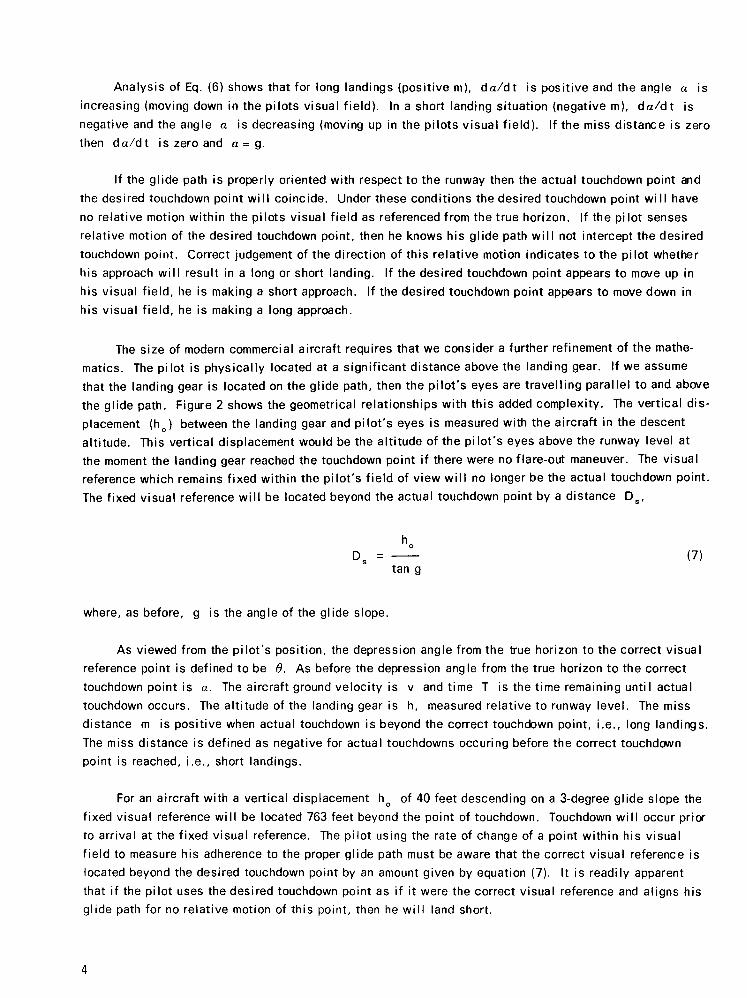
Analysis of Eq. (6) shows that for long landings (positive m), d a / d t is positive and the angle a is

increasing (moving down in the pilots visual f ield). In a short landing situation (negative m), d a / d t is

negative and the angle a is decreasing (moving up in the pilots visual f ield). If the miss distance is zero

then d a / d t is zero and a = g.

If the glide path is properly oriented with respect to the runway then the actual touchdown point and

the desired touchdown point wi l l coincide. Under these conditions the desired touchdown point wi l l have

no relative motion within the pilots visual f ield as referenced from the true horizon. If the pilot senses

relative motion of the desired touchdown point, then he knows his glide path wi l l not intercept the desired

touchdown point. Correct judgement of the direction of this relative motion indicates to the pilot whether

his approach wi l l result in a long or short landing. If the desired touchdown point appears to move up in

his visual f ield, he is making a short approach. If the desired touchdown point appears to move down in

his visual f ie ld, he is making a long approach.

The size of modern commercial aircraft requires that we consider a further refinement of the mathe­

matics. The pilot is physically located at a significant distance above the landing gear. If we assume

that the landing gear is located on the glide path, then the pi lot 's eyes are travelling parallel to and above

the glide path. Figure 2 shows the geometrical relationships with this added complexity. The vertical dis­

placement (ho) between the landing gear and pilot 's eyes is measured with the aircraft in the descent

altitude. This vertical displacement would be the altitude of the pi lot 's eyes above the runway level at

the moment the landing gear reached the touchdown point if there were no flare-out maneuver. The visual

reference which remains fixed within the pilot's f ield of view wi l l no longer be the actual touchdown point.

The fixed visual reference wi l l be located beyond the actual touchdown point by a distance D s ,

ho

Ds = — (7) tan g

where, as before, g is the angle of the glide slope.

As viewed from the pi lot 's position, the depression angle from the true horizon to the correct visual

reference point is defined to be 6. As before the depression angle from the true horizon to the correct

touchdown point is a. The aircraft ground velocity is v and time T is the time remaining until actual

touchdown occurs. The altitude of the landing gear is h, measured relative to runway level. The miss

distance m is positive when actual touchdown is beyond the correct touchdown point, i.e., long landings.

The miss distance is defined as negative for actual touchdowns occuring before the correct touchdown

point is reached, i.e., short landings.

For an aircraft with a vertical displacement ho of 40 feet descending on a 3-degree glide slope the

fixed visual reference wil l be located 763 feet beyond the point of touchdown. Touchdown wi l l occur prior

to arrival at the fixed visual reference. The pilot using the rate of change of a point within his visual

f ield to measure his adherence to the proper glide path must be aware that the correct visual reference is

located beyond the desired touchdown point by an amount given by equation (7). It is readily apparent

that if the pilot uses the desired touchdown point as if it were the correct visual reference and aligns his

glide path for no relative motion of this point, then he wi l l land short.

4

True Horizon

Correct

Actual

Correct

Fixed

Touchdown Point

Visual Reference

l , i j j r-r-r- , r >>>>•>>>*> t > j , ?j , , , , , , , , , , , , , , ,

—°s-H — °5-H - m •

• vT-

Fig. 2. Glide Path Geometry with Vertical Displacement.

From Fig. 2, the altitude of the pilot hp is

hn = h +h r (8)

and substituting Eqs. (1) and (7) then

hp = (vT + D s ) tan g (9)

The depression angle to the desired touchdown point a is

a = tan" (vT + DJ tan g

vT - m (10)

The rate of change of a is found by differentiating Eq. (10) and substituting Eq. (5),

da (m + D J v tan g (11]

d t ( v T - m ) 2 + (vT + D J 2 tan2 g

The depression angle to the correct visual reference 6 is

= tan"

(vT + D J tan g

( vT -m + D J (12)

The rate of change of 6 is found by differentiating Eq. (12) and substituting Eq. (5)

66 mv tan g (13)

dt ( v T - m + D J 2 + (vT + D J 2 t a n 2 g

Since the problem of short landings is of such immediate concern let us examine a case where the

glide path is properly aligned with the runway to affect touchdown at the desired point. If the pilot makes

no corrections to the glide path his miss distance wi l l be zero. However, let us assume that he is using

the desired touchdown point as his visual reference. Using Eq. (11) and m = 0 we find that

da

dT

Ds vtan g

m = 0 (vT)2 + (vT + D )2 tan2 g

(14)

and

da

d t

h„ v

m = 0 (vT)2 + (vT + D )2 tan2 g

(15)

Examination of Eq. (15) shows that the rate of change of a increases as the time until touchdown T

decreases. If at some point this rate of change exceeds the pilot 's threshold he wi l l interpret it as signal­

ing a departure from the correct glide path. Since a is increasing with time the touchdown point wi l l be

moving down in his visual f ield and he may well conclude that he is making a long landing. This erroneous

6

decision caused by using the desired touchdown point as a visual reference would lead to corrective action

to avoid the "long landing." The result would be a touchdown short of the desired touchdown point.

The rate of change of the depression angle of the desired touchdown point has been plotted in Fig. 3

for the case of a zero miss distance and pilot vertical displacement of 10 and 40 feet. Figure 3(a) is for a

3-degree glide slope at 200 mph while Fig. 3(b) is for the 3-degree glide slope at 135 mph. These rates in­

crease very rapidly as the range closes.

_e

20

15

10

05

3° Glide Slope h = Vertical Displacement

10 20

T (SECS)

(a) Ground Speed - 200 mph

10 20

T (SECS)

(b) Ground Speed - 135 mph

Fig. 3. Rate of Change of Touchdown Point for Correct Glide Pa th .

7

BLANK PAGE

2. COMPUTER GENERATED

LANDING FILM EXPERIMENT

An experiment was performed using Visibi l i ty Laboratory generated movies as visual stimuli. Its

purpose was to document the performance of observers charged with the task of judging adherence to a

specified glide path. The data from this experiment was used to determine thresholds of long-short judg­

ments. The information thus obtained is needed to analyze and predict conditions of weather and landing

geometries which would or could reduce, destroy, mask or change these visual cues to the extent that a

proper landing could not be made or that an improper landing would be made.

The observers were shown a series of computer-generated films depicting the last minute of descent

down a glide slope prior to touchdown. His a priori knowledge consists of the dimensions of a level run­

way, the glide slope, the ground speed, the rate of descent, and the location of the optimum touchdown

point. His visual task is to make subjective decisions as to whether the glide path in the film wi II inter­

cept the runway long or short of the desired touchdown point.

The films used as visual stimuli were generated at the Visibi l i ty Laboratory's computer image proces­

sing faci l i ty. The system software and hardware are nonreal time. The stimuli generated are therefore of

the "open-loop" type. This means that the observer can make judgments which can be recorded, but he is

unable to translate his judgments into actions which wi l l alter the dynamics of the situation.

9

2.1 RUNWAY BUILD PROGRAM

The runway build software program constructs a two-dimensional perspective view relative to the

horizon of a level rectangular runway as seen from an on-runway-axis location at a specific range and al t i ­

tude. Figure 4 shows pictorially what the software program creates. The scene generated is a stylized

runway devoid of any markings, numbers, or structural surroundings. The program requires as inputs:

1. Runway length

2. Runway width

3. Observer's altitude

4. Observer's distance from the end of the runway

5. Relative luminance of the sky

6. Relative luminance of the ground

7. Relative luminance of the runway

8. The location of the horizon in the scene

9. The angular resolution with which the scene is to be generated

10. Meteorological range, a number related to v is ib i l i ty which allows the program to

compute the proper contrast reduction for each portion of the f ield of view.

The images generated are displayed on a cathode ray tube and photographed with a 16mm Bolex

single frame movie camera. By starting with an appropriate altitude and distance and then properly incre­

menting both in accordance with the desired glide slope, the landing sequence f i lm is generated one frame

at a time. The landing is made short or long by choosing the starting altitude and range such that the glide

slope intercepts the runway long or short by the desired amount.

2.2 LANDING GEOMETRY

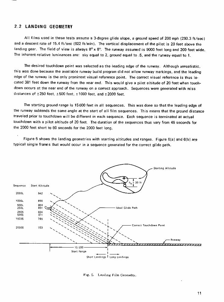
All films used in these tests assume a 3-degree glide slope, a ground speed of 200 mph (293.3 f t /sec)

and a descent rate of 15.4 ft/sec (922 ft/min). The vertical displacement of the pilot is 20 feet above the

landing gear. The f ield of view is always 8°x 8°. The runway assumed is 9000 feet long and 200 feet wide.

The inherent relative luminances are: sky equal to 2, ground equal to .5, and the runway equal to 1.

The desired touchdown point was selected as the leading edge of the runway. Although unrealistic,

this was done because the available runway build program did not allow runway markings, and the leading

edge of the runway is the only prominent visual reference point. The correct visual reference is thus lo­

cated 381 feet down the runway from the near end. This would give a pilot altitude of 20 feet when touch­

down occurs at the near end of the runway on a correct approach. Sequences were generated with miss

distances of ±250 feet, ±500 feet, ±1000 feet, and ±2000 feet.

The starting ground range is 15600 feet in all sequences. This was done so that the leading edge of

the runway subtends the same angle at the start of all fi lm sequences. This means that the ground distance

traveled prior to touchdown wi l l be different in each sequence. Each sequence is terminated at actual

touchdown with a pilot altitude of 20 feet. The duration of the sequences thus vary from 46 seconds for

the 2000 feet short to 60 seconds for the 2000 feet long.

Figure 5 shows the landing geometries with starting altitudes and ranges. Figure 6(a) and 6(b) are

typical single frames that would occur in a sequence generated for the correct glide path.

Start ing A l t i t ude

1000S

2000S

Sequence Start A l t i t ude

2000L 942

1000L 890

BOOL 250L

864 851 0 2

250S 500S

824 811

Short Landings I Long Landings

Fig. 5. Landing Film Geometry.

11

(a) Range 15600 ft (b) Range 3800 ft

Fig. 6. Computer Generated Runway, Ideal Glide Path.

We are interested in the angle from the horizon to the correct visual reference 0 and the rate of

change of this angle with respect to the time remaining until touchdown T. These equations were derived

earlier as Eqs. (12) and (13) and are plotted in Figs. 7 and 8 for the eight miss distances used in the

pyschophysics experiment. -

5 I 1 1 1 1 1 1

500L 1000L 2000L

0 10 20 30 40 50 60

T (SECONDS)

Fig. 7. Angle to Correct Visual Reference.

12

.020

.015

.010

.005 o UJ </i

u a o •5 \ •o

-.005

-.010

-.015

-.020

Fig. 8. Rate of Change of Correct Visual Reference.

The leading edge of the runway, the desired touchdown point, is a prominent, easily identified, fixa­

tion point. The angle a from the horizon to the leading edge of the runway was derived as Eq. (10), and

the rate of change of this angle with the time remaining until touchdown was derived as Eq. (11). Equa­

tions (10) and (11) are plotted in Figs. 9 and 10 for the eight miss distances used in the experiment.

2.3 EXPERIMENTAL TECHNIQUE

A free choice technique was used. The observers were requested to make high confidence decisions

even though they knew that every approach was either long or short. A complete data run consists of ten

random presentations of each landing configuration, a total of 80 landing approaches. The data run was

divided into four separate 20-minute sessions.

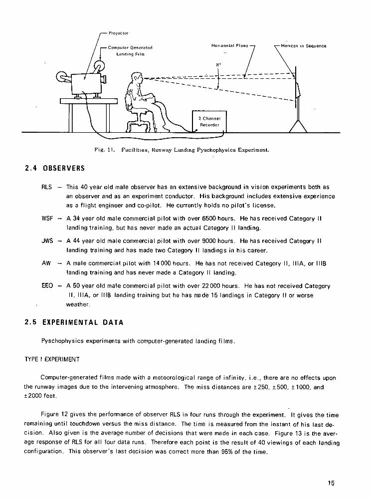
The observer is located so that the presentation on the screen subtends a f ield of view that is

8°x 8°. The horizon in the film and the eyes of the observer are located in a horizontal plane. Figure 11

shows the faci l i t ies used in the experimental setup. The observer operates a three-position toggle switch

which is time synchronized with the film presentation. Since the center position indicates no decision,

the observer uses the switch to indicate whether he believes the landing wi l l be long or short. The

observer operates the switch throughout the complete sequence so that a time record of his responses

from start to finish is made.

13

4 —

3 —

2 —

1 —

250L 500L 1000L r i

2000L

1 1

250S ^ , " ^ , 250S ^ , " ^ , 250S ^ , " ^ ,

' i l l l l ^ ^

1 0 0 0 S > ^ ^ * *

2000SyT 3° Glide Slope 200 mph

1 1 1 1 1 10 20 30

T (SECONDS)

40 50 60

Fig. 9. Angle to Correct Touchdown Point .

.020

.015

.010 —

.005 —

-.005

•010

.015

-.020

T (SEC

500S

Fig. 10. Rate of Change of Correct Touchdown Point .

14

• Projector

Horizon in Sequence

Fig. 11. Facilities, Runway Landing Pyschophysics Experiment.

2.4 OBSERVERS

RLS — This 40 year old male observer has an extensive background in vision experiments both as

an observer and as an experiment conductor. His background includes extensive experience

as a flight engineer and co-pilot. He currently holds no pilot 's license.

WSF - A 34 year old male commercial pilot with over 6500 hours. He has received Category II

landing training, but has never made an actual Category II landing.

JWS - A 44 year old male commercial pilot with over 9000 hours. He has received Category II

landing training and has made two Category II landings in his career.

AW - A male commercial pilot with 14 000 hours. He has not received Category I I , IIIA, or 1MB

landing training and has never made a Category II landing.

EEO — A 50 year old male commercial pilot with over 22 000 hours. He has not received Category

I I , IIIA, or 1MB landing training but he has made 15 landings in Category II or worse

weather.

2.5 EXPERIMENTAL DATA

Pyschophysics experiments with computer-generated landing fi lms.

TYPE I EXPERIMENT

Computer-generated films made with a meteorological range of infinity, i.e., there are no effects upon

the runway images due to the intervening atmosphere. The miss distances are ±250, ±500, ±1000, and

±2000 feet.

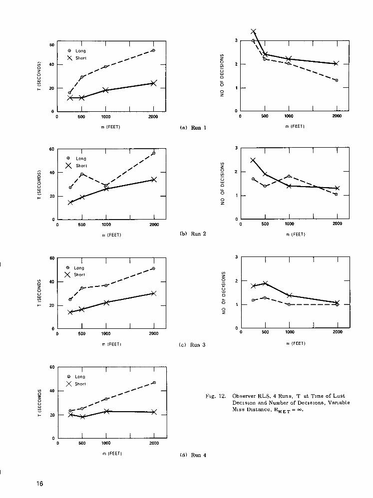
Figure 12 gives the performance of observer RLS in four runs through the experiment. It gives the time

remaining until touchdown versus the miss distance. The time is measured from the instant of his last de­

cision. Also given is the average number of decisions that were made in each case. Figure 13 is the aver­

age response of RLS for all four data runs. Therefore each point is the result of 40 viewings of each landing

configuration. This observer's last decision was correct more than 95% of the time.

15

Q 2 o

60 I I I ! © Long ^,JS>

X Short ^ » - ^ ^ "

411 *&"

.*-^^ f ~ / T^

20

1 1 1 1 500 1000

m (FEET)

2000

Z O

U u j Q

O 2

(a) Run 1

o 2 O o

60

40

_ 20 -

1 ® Long

X Short

1 1 i

s

4 ^

1 1 1 1 500 1000

m (FEET)

2000

o uj Q u. O O

(b) Run 2

Q 2 O (J

O u j D

O 2

(c) Run 3

Fig. 12. Observer RLS, 4 Runs, T at Time of Last Decision and Number of Decisions, Variable Miss Distance, R M E T = °°.

(d) Run 4

16

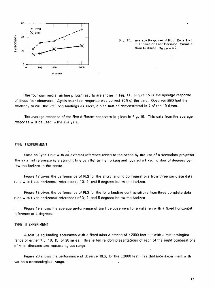
Fig. 13., Average Response of RLS, Runs 1 — 4, T at Time of Last Decision, Variable Miss Distance, R M E T = <»'

0 500 1000 2000

m (FEET

The four commercial airline pi lots' results are shown in Fig. 14. Figure 15 is the average response

of these four observers. Again their last response was correct 95% of the time. Observer EEO had the

tendency to call the 250 long landings as short, a bias that he demonstrated in 7 of the 10 times.

The average response of the five different observers is given in Fig. 16. This data from the average

response wi l l be used in the analysis.

TYPE II EXPERIMENT

Same as Type I but with an external reference added to the scene by the use of a secondary projector.

The external reference is a straight line parallel to the horizon and located a fixed number of degrees be­

low the horizon in the scene.

Figure 17 gives the performance of RLS for the short landing configurations from three complete data

runs with fixed horizontal references of 3, 4, and 5 degrees below the horizon.

Figure 18 gives the performance of RLS for the long landing configurations from three complete data

runs with fixed horizontal references of 3, 4, and 5 degrees below the horizon.

Figure 19 shows the average performance of the five observers for a data run with a fixed horizontal

reference at 4 degrees.

TYPE III EXPERIMENT

A test using landing sequences with a fixed miss distance of ±2000 feet but with a meteorological

range of either 7.5, 10, 15, or 20 miles. This is ten random presentations of each of the eight combinations

of miss distance and meteorological range.

Figure 20 shows the performance of observer RLS, for the ±2000 feet miss distance experiment with

variable meteorological range.

u u

40 — Q 2 O U

t- 20 —

I I I I 0 Long js X Short ^ ^ ^

I I I I

17

60

40

20 —

1

_ • af*

1 1 -i —

© Long

—

X Short 1 1 1

o u j

a u. O

6

500 1000

m (FEET)

2000

<a) Observer WSF

z o

o UJ

•

o z

(b) Observer JWS

z o

Q u-O

O z

(c) Observer AW

z o

u UJ

o

o z

(d) Observer EEO

Fig. 14. P i lo t Observers , T at Time of Las t Decision and Number of Decis ions , Variable Miss Dis tance , R M E T = °°.

o u o

Fitf. 15. Average Response of Four Pilot Observers, T at Time of L a s t Decision, Variable Miss Distance, R M E T = oo.

Fig. 16. Average Response of Five Observers, T at Time of Las t Decision, Variable Miss Dis tance, R M E T = °°.

o z o u

60

Q z o u

20 —

1 3 Long

I

3 1 . - " -** >®Tn

— *r S 4° ^, • "

fr' > " 9

l 1 1 1 500 1000

m (FEET)

2000

Fig. 17. Observer RLS, with External Reference, T at Time of Las t Decision, Variable Short Miss Distance, R M E T = oo.

Fig. 18. Observer RLS, with External Reference, T at Time of Las t Decision, Variable Long Miss Dis tance, RM . , _ = oo.

Q Z o o

o

60

40 —

20

1 © Long

X Short

1 1 1 . - -<S>- - ©

© - ^ ^ 2000L

— . . , itf —

> H 2000S

1 1 1 1 5 10 15 20

METEOROLOGICAL RANGE (MILES)

Fig. 19. Average Response of Four P i lo t s ,

Variable Miss Distance, R, MET

External Fig. 20. Observer RLS, T at Time of Las t Decision, Variable Meteorological Range, 2000-Foot

oo, 1 Run. Miss Dis tance.

19

2.6 ANALYSIS

If the observer was uti l izing the displacement of either the correct visual reference or the leading

edge of the runway as a primary visual cue his subjective decisions should all occur when his fixation

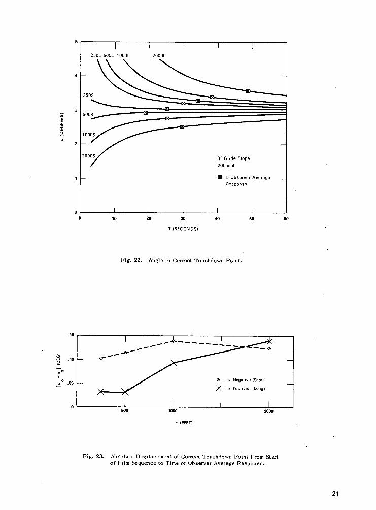
point has changed by some finite amount. In Figs. 21 and 22 the five observers average data from Fig. 16

has been indicated on the curves of Figs. 7 and 9 which show the angles to the correct visual reference

and the end of the runway.

500L 1000L 2000L

B 5 Observer Average Response

0 10 20 30 40 50 60

T (SECONDS)

Fig. 21. Angle to Correct Visual Reference.

Each of the computer-generated movies started at a time before touchdown which is a function of the

magnitude of the touchdown error. For this reason Figs. 21 and 22 do not clearly indicate the change in

angular location which has taken place between the start of the film and the time of final decision. Fig.

23 is a plot of the absolute magnitude of this angular change as a function of the miss distance. It is of

considerable interest to note that 6 of the 8 averaged data points fall within the relatively narrow range

between 0.095 and 0.14 degrees.

(/) UJ UJ

cr UJ

Q

20

13 u j Q

250L 500L 1000L 2000L

2B0S

500S

1000S

2000S

10 20

3° Glide Slope 200 mph

E3 5 Observer Average Response

30

T (SECONDS)

40 50 60

Fig. 22. Angle to Correct Touchdown Point .

.15

.05 —

X-© m Negative (Short)

X m Postivie (Long)

500 1000

m (FEET)

2000

Fig. 23. Absolute Displacement of Correct Touchdown Point From Start of Film Sequence to Time of Observer Average Response .

21

The dynamic visual cue was investigated by indicating the average observer from Fig. 16 on the

curves of Figs. 8 and 10 which show the rate of change of the angles to the correct visual reference and

the end of the runway. These are shown in Figs. 24 and 25.

.020

.015

.010

.005

-.005

.010

-.015

-.020

UJ

Q

.020

.015

.010

.005

-.005

-.010

.015 —

.020

T (SECONDS)

500S / 2000S Response

/ I / • / I

Fig. 24. Rate of Change of Correct Visual Reference. Fig. 25. Rate of Change of Correct Touchdown Point.

It should be remembered that the stylized runway in the experiments had no physical identification

of the correct visual reference that the observers could use for visual f ixation. The closest identifiable

fixation point would be the leading edge of the runway which was designated as the correct touchdown

point. If the subjective decisions were based solely on the observers ability to sense a rate of change

in the correct touchdown point then the experimental data points would all fal l on the appropriate curve

at the same absolute rate of change. Examination of Fig. 25 shows that the last decision took place at

times where the rate of change of the correct touchdown varied from .0030 to .0135 degrees per second.

An interesting check on the data can be obtained by assuming a fixed threshold for rate of change

of the leading edge of the runway and calculating expected performance. The curve shown in Fig. 26 was

made by calculating the time T at which the absolute rate of change would be .01 degrees per second.

This theoretical curve is a reasonable match to the average observer curve in Fig. 16. Since the geometry

dictates that the 250-foot short case wi l l reach the .01 degrees per second rate before the 500-foot short

case, because of the offset of the visual axis from the wheels, there is a rational reason for the observer

to show earlier detection of the 250-foot short landing than the 500-foot short landing.

22

60

in 40 Q Z o

_ 20 — -K

1 I 1 ^ x ^ Long

^^0*-*"^ Short

1 I 1 1

Fig. 26. Theoretical Response Time for d a / d t = .01 Deg/Sec , R M E T = oo.

500 1000

m (FEET)

2000

Analysis of Figs. 17, 18, and 19 confirms that the addition of a stable horizontal reference to the

scene improves the ability of the observer to make correct subjective decisions about the glide path. It

is apparent that the closer this external reference is to the place where the observer is f ixating, the

easier the visual task.

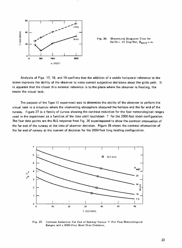
The purpose of the Type III experiment was to determine the ability of the observer to perform his

visual task in a situation where the intervening atmosphere obscured the horizon and the far end of the

runway. Figure 27 is a family of curves showing the contrast reduction for the four meteorological ranges

used in the experiment as a function of the time until touchdown T for the 2000-foot short configuration.

The four data points are the RLS response from Fig. 20 superimposed to show the contrast attenuation of

the far end of the runway at the time of observer decision. Figure 28 shows the contrast attenuation of

the far end of runway at the moment of decision for the 2000-foot long landing configuration.

6 —

4 —

3 —

Fig. 27. Contrast Reduction Far End of Runway Versus T For Four Meteorological Ranges and a 2000-Foot Short Miss Dis tance.

23

5 —

20 30 40

T (SECONDS)

Fig. 28. Contrast Reduction Far End of Runway Versus T For Four Meteorological Ranges and a 2000-Foot Long Miss Dis tance .

Examination of Figs. 27 and 28 does not show a marked dependence of decision time upon contrast

reduction of the far end of the runway, however, it should be noted that the contrast transmittance values

were not low enough to badly obscure the far end of the runway.

24

3. INTRODUCTION TO MOTION DETECTION THRESHOLD EXPERIMENT

The results of the experiments performed with the computer-generated movies seem to suggest that

the observer is able to sense that he is long or short in his landing when the leading edge of the runway

has moved in angular space by an amount equal to something on the order of 0.1 degrees. In an effort to

provide additional independent testing of this hypothesis, an experiment was performed using a horizontal

line displayed on a cathode-ray-tube to measure the angular thresholds for detection of motion.

3.1 EXPERIMENTAL TECHNIQUE

The visual stimuli was presented to the observer in a uniform field of view of 8°x 8°. This size

display is identical to the f ield of view used in the landing film experiments. The 8°x 8° f ie ld was cen­

tered in another uniform field of view of 30°to insure that no bias is introduced by extraneous visual

references such as the control knobs on the display scope.

Each data run consists of a series of presentations where the line moves away from a starting

position do with a constant velocity. After each presentation the display is returned to the starting

position and after a five second pause the next presentation occurs. Both starting position and the hori­

zontal width of the line are a constant for a complete data run.

The observer's task is to make a judgment as to the direction of travel of the horizontal line. He

is instructed to make high confidence decisions but to respond as soon as he has consciously made a

choice. It is a free choice experiment and he can change his decision at any time in the presentation.

The start of a presentation is indicated by the cessation of an audio signal.

The observer responses are made with a three position toggle switch spring loaded to the no

decision position. His decisions and the rate of motion in the display are recorded on a two-channel

time synchronized recorder in a manner similar to that used for the computer-generated landing sequences.

25

The data desired is the average time from the start of the presentation to the instant when the ob­

server makes the correct decision as to the direction of travel.

Figure 29 is a block diagram of the equipment used in the experiment. Figure 30 shows the arrange­

ment of the faci l i t ies.

DISPLAY

WIDTH

CONTROL

DISPLAY

WIDTH

CONTROL

r> / dt r> / dt

DISPLAY SCOPE

RATE

DEPENDENT

VOLTAGES

RANDOM

VOLTAGE

SELECTOR

V (

INTEGRATOR

r> / dt Horz In

Vert In

Posi t ion

RATE

DEPENDENT

VOLTAGES

RANDOM

VOLTAGE

SELECTOR

V (

INTEGRATOR

r> Horz In

Vert In

Posi t ion

RATE

DEPENDENT

VOLTAGES

RANDOM

VOLTAGE

SELECTOR

V (

INTEGRATOR

r> Horz In

Vert In

Posi t ion

RATE

DEPENDENT

VOLTAGES '

RANDOM

VOLTAGE

SELECTOR

INTEGRATOR

Horz In

Vert In

Posi t ion

RATE

DEPENDENT

VOLTAGES

RANDOM

VOLTAGE

SELECTOR

INTEGRATOR

Horz In

Vert In

Posi t ion

RATE

DEPENDENT

VOLTAGES

RANDOM

VOLTAGE

SELECTOR

INTEGRATOR

Horz In

Vert In

Posi t ion

»o RECORDER

d 0 / d t

Response OBSER

RESPO

i/ER

d 0 / d t

Response OBSER

RESPO JSE

d 0 / d t

Response

Fig. 29. Block Diagram, Motion Threshold Experiment.

UNIFORM FIELD MASK

EXPERIMENT

OPERATOR

CONTROLS

Fig. 30. Facilities, Motion Threshold Experiment.

26

3.2 DATA AND ANALYSIS

The first run was conducted with observer RLS and the line equal to the width of the display 8° and

always starting in the middle 6o = 4° The results are shown in Fig 31(a) A theoretical curve has been

added to all four graphs in this figure which indicated the performance which would correspond to detec­

tion of an angular change of 0 1 degrees

0 02 04 06 08 10 0 02 04 06 08 10

dfl /dt (DEG/SEC) dfl /dt (DEG/SEC)

(a) OBSERVER RLS 0 = 4 ° WIDTH 8° (b) OBSERVER RLS 0 - 4° WIDTH 2° o o

0 02 04 06 08 10 0 02 04 06 08 10

dfl /dt (DEG/SEC) dr /dt (DEG/SEC )

(c) OBSERVER GDE 0 = 4° WIDTH 2° (d) OBSERVER RLS fl = 6 ° WIDTH 2° o o

Fig 31 . Data, Motion Threshold Experiment.

27

It was then decided to reduce the width of the horizontal display line to more closely match the

angular subtense of the stylized runway used in the runway landing experiment. Two degrees were chosen

as the angle the 200-foot wide runway would subtend at a ground range of 11 457 feet. Three sessions of

100 presentations each were then conducted with observer RLS, thus giving us 30 trials for each of the

ten data points (5 rates and 2 directions). This data is shown in Fig. 31(b). Observer GDE participated

in one session of 100 presentations and the results are shown in Fig. 31(c).

It was then decided to move the starting point of the line closer to the lower edge of the display.

This was done in an attempt to check the dependency of the response upon the angular distance to the

closest fixed visual reference. The data for observer RLS with a starting point 6° from the top of the dis­

play is given in Fig. 31(d).

Figures 31(a), (b), (c), and (d) generally support the hypothesis that detection wi l l occur when the

line has moved by an amount on the order of 0.1 degrees which is in turn consistent with the hypothesis

that the judgments of long and short landings in the computer-generated movies were made based upon

angular movement of the leading edge of the runway.

Although the number of observations is relatively small, it is interesting to note that the two ob­

servers had opposite preferential capability with reference to the direction of motion of the line.

28

4. INTRODUCTION TO DAYTIME FOG PROGRAM

Bad weather is a contributing factor in many aircraft landing accidents. Continued study of the visual

function during landing requires that computer software programs be developed which allow the effects of

bad weather to be added to a scene. These programs can then be used both in analytic studies and in gen­

eration of visual stimuli for psychophysics experiments.

Fog is one of the most severe and important conditions related to aircraft landings and bad weather.

Therefore, a software program has been developed to duplicate the effects of fog upon any scene, the

scene being stored in the computer as a two-dimensional array of relative luminance values.

4.1 THEORY FOR DAYTIME FOG PROGRAM

There are a number of factors involved in the reduction of image quality imposed by transmission of

the light through fog. The purpose of this section is to discuss very briefly the nature of these processes

and to indicate the equations which are the basis of the computer program for insertion of fog in daytime

scenes.

Light is emitted or reflected from a point on the object of interest in such a way that it travels

toward the observer. Some of this light encounters the water droplets of the fog and is scattered. If we

assume that light which is scattered is no longer useful for image formation, then the image is determined

by knowing what portion of the light is transmitted without undergoing scatter. If the inherent luminance

of the scene is B0 then the unscattered component at a distance R wi l l be

BR = B0 e _ a R , (16)

where a is the attenuation coefficient. The constant a is the sum of both scattering and absorption co­

efficients, although the literature seems to indicate that the absorption of most fogs is small.

29

Some of the light which is scattered by only a small angle wi l l st i l l reach the observer. This is

apparent in the nighttime viewing of a small light source where one can see the glow surrounding the light.

During the daytime this glow component wi l l not be apparent, and wi l l generally be numerically negligible

and is therefore neglected. This simplification does restrict this computer program to daytime use. A

nighttime program can and probably wi l l be written, but wi l l be more complex and wi l l require more com­

puter time for execution.

The other important factor in the deterioration of image quality by fog is the addition of path lumi­

nance. Path luminance is ambient light which has been scattered by the fog in a direction toward the

observer such that it appears to be coming from the object. For a viewing situation which is homogeneous

both with respect to transmission properties and lighting geometry, the path luminance also obeys the ex­

ponential and asymptotically approaches a value called equilibrium luminance BQ when the range is

large. Mathematically,

B * = BQ (1 - e-QR) . (17)

The total luminance of the path of sight is the sum of Eqs. (16) and (17), or

B = B e~ a R +B n ( 1 - e ~ a R ) . (18)

Equation (18) is the basis of the Daytime Fog Computer Program.

4.2 COMPUTER PROGRAM

Assume that a clear weather photograph is taken of a runway scene as viewed from some point along

the approach path. This photograph is then scanned and digitized for entry into the computer. The job of

the computer program is to operate upon this numerical image in such a way as to produce a new computer

image appropriate to viewing through a specified fog condition.

Figure 32 wi l l be used in the derivation for the range at a point in the array. The origin is defined

in the upper left-hand corner of the array. The optical axis OH of the camera system is parallel to the

horizontal plane at an altitude h and is perpendicular to the fi lm plane. The infinity point in the array

H' is located at point I,J. Let us define a point P somewhere on the horizontal plane which maps onto

point P' in the array. P' is located at point i , j .

If the film were taken with a focal length of F and if the scanning aperture used to generate the

array is the same in both directions, i.e., Ax = Ay = A, then each element in the array subtends an angle

of 6 where

A 6 = 2 t a n - 1 — . (19)

2F

30

• Optical Axis

Fig. 32. Range for Runway Build Program

The unmagnified film should be viewed from a distance OH' equal to the focal length

OH' = F . (20)

The distance between any two points, i2 , j2 and i j j , , in the array is

lengthy = [ A 2 ( ! 2 - i ,)* + A2(\2 - j , ) ' ] (21)

Therefore, the length of H'P' in the array is

H'P' = A2(i - l ) ' + A2(j - J ) r (22)

and the length of OP' can be found as

OP' = (OH')2 + (H'P') (23)

31

Substituting Eqs. (20 and (22) into Eq. (23)

OP' = | F 2 + A2(i - l ) 2 + A2( j - J ) 2 | * . (24)

The range to the point P is OP. Using the geometry of similar triangles and knowing the altitude h at

which the film was taken, thus

OP h

OP' H'R (25)

but

H'R' = A(j - J ) , (26)

and therefore the range to point P is

OP = f F2 + A2(i - I)2 + A2( j - J ) 2 | ^ . (27) A(j - J )

At each point in the array there wi l l be a luminance B0(i,j). The program wi l l replace this lumi­

nance with BR(i,j), when j > J

BR(i,j) = B 0 ( i , j ) e - a R i i + B Q ( 1 - e ~ a R . i ) , (28)

and

R.. = h [F2 + A2(i - l ) 2 + A2( j - J ) 2 ] * , (29) " A ( j - J )

[F2 + A2(i - l ) 2 + A2( j - J ) 2 ]

32

and when j < J

BR(U) = B0 , (30)

since

R -

4 . 3 RUNWAY V I S I B I L I T Y RANGE (RVR) A N D ALPHA ( a )

The RVR is defined as the distance at which a standard observer can detect runway lights of a given

intensity I. The limit of detection is set by the illumination threshold of the eye according to the rela­

tionship by Allard

where

I Et = — e " a R (31)

R2

E, = Illuminance threshold cd/m2

I = Intensity of lights (cd)

R = Distance (m)

a = Attenuation coefficient (m_1)

However, the illumination threshold Et is related to the background luminance. As reported by

D. C. Thomas,2 the Blind Landing Experiment Unit, a part of the Royal Aircraft Establishment, has postu­

lated the relationship as

log Et = -5 .7 + .64 log B (32)

where B = background luminance cd/m2 .

Equations 31 and 32 can be combined to solve for the attenuation coefficient a,

log I +5.7 - .64 log B - 2 log R a = ——

R log e (33)

2. J. Sci. & Technology, Vol. 37, No. 2, 1970.

33

The high intensity runway edge lights used today have an intensity of 20000 candles. Therefore, to select

the proper attenuation coefficient a to use in the daytime fog program, the background illuminance and

the RVR of the scene must be known.

4.4 REAL FOG AND COMPUTER-GENERATED FOG

On 26 April 1973 Visibi l i ty Laboratory personnel made photographs and measured background lumi­

nance in the FAA/NASA Low Visibi l i ty Research Facility at the Richmond Field Station in Richmond,

California. This occurred during a test being conducted by NASA-Ames personnel. A Gamma Scientific

photometer with a two-degree f ield of view was used to measure the background luminance looking down

the runway at various elevation angles. Measurements were made in the clear and with fogs having RVR's

of 2400, 1200, 700, and 300 feet. This data is plotted in Fig. 33. Photographs were made at the same

time looking down the runway from the aircraft cockpit. The photographs were returned to the Visibi l i ty

Laboratory and scanned with the Optronics Scanner to get the two-dimensional arrays.

1000

u z <

o

<

X - K Clear

O-^ ) 2400 ft RVR

/ V - A 1200 ft RVR

• — D 700 ft RVR

300 ft RVR

Fog Chamber Axis

Cockpit Photometer

-10 0 10

ELEVATION ANGLE (DEGREES)

20

Fig. 33. Background Luminance, Richmond Field Station Fog Chamber, HIRL Step 5, 26 April 1973, 1700 Hours.

34

Figure 34 is the original photograph taken without fog. Selecting a background luminance value of

684 cd/m2 from Fig. 32, the attenuation coefficients a were calculated corresponding to RVR's of

2400 feet RVR, a =

1200 feet RVR, a =

700 feet RVR, a =

300 feet RVR, a =

.00774 M _ 1

.01925 M _ 1

.03805 NT1

.10925 M" 1

Fig. 34. FAA/NASA Low Visibili ty Research Faci l i ty Runway, Clear Atmosphere.

The original runway scene was then processed using the daytime fog program to add fog to the array.

The pictures taken in the fog chamber are shown for comparison to the results of the daytime

fog program,

Figure 35 RVR of 2400 feet

35

Figure 36

Figure 37

Figure 38

36

RVR of 1200 feet

RVR or 700 feet

of 300 feet

It is believed that the ability to generate computer pictures which accurately portray viewing situations

through fog can be an important tool in the quantitative evaluation of the visual stimulus involved in bad

weather landings.

37

BLANK PAGE

38

5. SUMMARY AND CONCLUSIONS

The intent of the landing studies was to attempt to determine the nature of the visual stimulus of

importance to the pilot and to quantitatively define his threshold judgments of long and short landings

The experiments performed in connection with these studies tend to suggest that long and short judg­

ments are based upon an angular change of the leading edge of the runway with the threshold of this

change being on the order of 0 1 degrees The data for the 250 and 500 foot short landing cases did

not f i t this pattern and as of the time of writing this report no explanation of these deviations has

been discovered

The independent experiment using a moving line on a catrode-ray-tube served two useful purposes

First of all it tended to confirm a visual threshold corresponding to a total angular movement on the order

of 0 1 degrees This tends to substantiate the idea that the long-short judgments are based upon motion

of the leading edge of the runway and are independent of the presence of the horizon and/or the changing

geometric pattern formed by the runway The experiment was also useful in that it did not involve either

the discrete resolution of the computer pictures nor the discrete frame-by-frame presentation of the movie

camera This suggests that neither the discrete resolution nor the discrete frame-by-frame presentation

adversely affected this experimental determination of the motion thresholds

The computer program which was written to insert fog into photographs of runway scenes has been

shown to be capable of generating very realistic fog viewing It is believed that this program wi l l be of

great value in studying the problems of visual stimulus during low-ceiling, - l ow visibi l i ty landing

situations

iv

39

BLANK PAGE

40

APPENDIX

COMPUTER FACILITY

The Visibi l i ty Laboratory computer installation, shown in Fig. 39 and 40, is an IBM System 360/44.

The physical characteristics of the IBM 360/44 are listed below.

UNIT DESCRIPTION

2044 Central Processing Unit with 1 microsecond,

32K 32-bit word core and disk storage of 1 x 10b bytes.

1442 Card Read-Punch, 400 cards/minute.

1443 Line Printer, 240 lines/minute.

2415 Magnetic Tape Unit, two drives, nine track,

15 000 bytes/second.

2841 Disk Storage Control.

2311 Disk Drive with 1316 cartridge, 7 x 106 bytes.

2701 Data Adapter Unit.

2741 Communication Terminal:

One 16-bit A/D converter

Two 16-bit contact operate banks

Three 16-bit digital input groups

Two 13-bit D/A converters

41

Fig. 39. The IBM System 360 / 44 Computer.

Fig. 40. The IBM System 360/44 Computer and the Refresh Display Console .

42