probabilistic and numerical validation of …

PROBABILISTIC AND NUMERICAL VALIDATION OFHOMOLOGY COMPUTATIONS FOR NODAL DOMAINS

SARAH DAY, WILLIAM D. KALIES, KONSTANTIN MISCHAIKOW,AND THOMAS WANNER

Abstract. Homology has long been accepted as an important computabletool for quantifying complex structures. In many applications these structures

arise as nodal domains of real-valued functions and are therefore amenable

only to a numerical study, based on suitable discretizations. Such an approachimmediately raises the question of how accurate the resulting homology com-

putations are. In this paper we present a probabilistic approach to quantifying

the validity of homology computations for nodal domains of random Fourierseries in one and two space dimensions, which furnishes explicit probabilistic a-

priori bounds for the suitability of certain discretization sizes. In addition, we

introduce a numerical method for verifying the homology computation usinginterval arithmetic.

1. Introduction

The practical need to extract low-dimensional nonlinear structures from high-dimensional data sets has led to the introduction of topological methods in statis-tical analysis, and currently there is a growing body of literature [22, 25, 10, 9, 6]that addresses the following problem: provide efficient algorithms for estimatingtopological properties of an unknown manifold X given a point-cloud data set thatlies on or near X. It should be mentioned that for some of the proposed applicationsit is reasonable to assume that the point-cloud data set is obtained via a randomsampling process.

To a large extent the emphasis of the above-mentioned papers is on the methodof estimation. From now on we restrict our attention to homology where to thebest of our knowledge the first result concerning the accuracy of such estimationis due to Niyogi, Smale, and Weinberger [21]. In this paper, the authors propose astochastic algorithm for computing the homology of a given manifold X ⊂ Rd byrandomly sampling M points from the manifold, and derive explicit bounds on theprobability that their algorithm computes the correct homology. The probabilitybound depends on the number M and a condition number 1/τ . The latter param-eter encodes both local curvature information of the manifold X, as well as global

Date: November 14, 2006.1991 Mathematics Subject Classification. Primary 60G60, 55-04; Secondary 55N99, 60G15.

Key words and phrases. Homology, random Fourier series, nodal domain.Sarah Day was partially supported by NSF grant DMS-9983660 at Cornell University and NSF

grant DMS-0441170 at MSRI. .William Kalies was partially supported by NSF grant DMS-0511208 and DOE grant 97888.

Konstantin Mischaikow was partially supported by NSF grants DMS-0511115 and DMS-0107396, by DARPA, and by DOE grant 97891.

Thomas Wanner was partially supported by NSF grant DMS-0406231 and DOE grant 97889.

1

2 S. DAY, W.D. KALIES, K. MISCHAIKOW, AND T. WANNER

separation properties. More precisely, the inverse condition number τ is the largestnumber such that the open normal bundle about X ⊂ Rd of radius r is embeddedin Rd for all r < τ .

Consider now the problem of an evolutionary system which produces complicatedspatial patterns, such as for example phase separation in materials, turbulent fluidflow, predator-prey populations in spatially explicit systems, etc. Again, theseare typically high-dimensional systems for which there is considerable interest inunderstanding the temporal changes of the low-dimensional nodal domains, i.e.,patterns, and homological methods appear to provide new techniques through whichone can explore these problems [13, 14, 18]. Notice, however, that in this settingthe topology of the level sets which define the nodal domains changes as a functionof time, and thus, there is no fixed manifold X for which one is trying to computethe homology. Furthermore, as the topology changes the condition number 1/τbecomes unbounded.

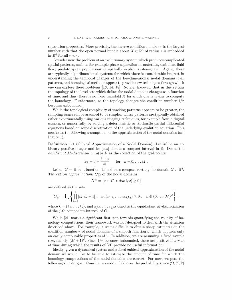
While the topological complexity of tracking patterns appears to be greater, thesampling issues can be assumed to be simpler. These patterns are typically obtainedeither experimentally using various imaging techniques, for example from a digitalcamera, or numerically by solving a deterministic or stochastic partial differentialequations based on some discretization of the underlying evolution equation. Thismotivates the following assumption on the approximation of the nodal domains (seeFigure 1).

Definition 1.1 (Cubical Approximation of a Nodal Domain). Let M be an ar-bitrary positive integer and let [a, b] denote a compact interval in R. Define theequidistant M -discretization of [a, b] as the collection of the grid points

xk = a +b− a

M, for k = 0, . . . ,M .

Let u : G → R be a function defined on a compact rectangular domain G ⊂ Rd.The cubical approximations Q±M of the nodal domains

N± = x ∈ G : ±u(t, x) ≥ 0are defined as the sets

Q±M =⋃

d∏`=1

[k`, k` + 1] : ±u(x1,k1 , . . . , xd,kd) ≥ 0 , k ∈ 0, . . . ,Md

,

where k = (k1, . . . , kd), and xj,0, . . . , xj,M denotes the equidistant M -discretizationof the j-th component interval of G.

While [21] marks a significant first step towards quantifying the validity of ho-mology computations, their framework was not designed to deal with the situationdescribed above. For example, it seems difficult to obtain sharp estimates on thecondition number τ of nodal domains of a smooth function u, which depends onlyon easily computable properties of u. In addition, we are assuming a fixed samplesize, namely (M + 1)d. Since 1/τ becomes unbounded, there are positive intervalsof time during which the results of [21] provide no useful information.

Ideally, given a dynamical system and a fixed cubical approximation of the nodaldomain we would like to be able to estimate the amount of time for which thehomology computations of the nodal domains are correct. For now, we pose thefollowing simpler goal. Consider a random field over the probability space (Ω,F , P)

VALIDATION OF HOMOLOGY COMPUTATIONS 3

Figure 1. Nodal domains of a random trigonometric polynomialin two space dimensions and their cubical approximations withM = 50.

and the compact rectangular domain G ⊂ Rd. Let M be an arbitrary positiveinteger. Approximate the random nodal domains N±(ω) of the realization u(·, ω) :G → R by cubical sets Q±M (ω) as in Definition 1.1. We are interested in thefollowing problem:

(P) Find sharp lower bounds on the probability

Pω ∈ Ω : H∗

(N±(ω)

) ∼= H∗(Q±M (ω)

)as a function of M .

As is made clear in this announcement, we approach this problem from two distinctpoints of view. The first, which is discussed in Section 2, is to obtain probabilisticlower bounds. Since it is not a priori clear that these bounds are sharp, in Sec-tion 3 we describe a numerical procedure to rigorously determine when for a givensufficiently smooth u : G → R we have H∗ (N±) ∼= H∗

(Q±M

).

We conclude this paper in Section 4 by applying the probabilistic and numericaltechniques to two problems. The first is to determine the number of subdivisions,M , needed in order to guarantee with high probability that the homology of thenodal domain of a random trigonometric polynomial is computed correctly usinga cubical approximation. The second is to study the patterns produced by thestochastic Cahn-Hilliard model for phase separation in binary alloys.

2. Probabilistic Estimates

Random fields and in particular random Fourier series have been studied exten-sively during the last few decades. See for example [1, 2, 12, 16, 19], as well as thereferences therein. With this in mind, we present an abstract probability estimatefor general random fields. Then using this abstract result we consider, separately,the case of random Fourier series for one and two space dimensions.


2.1. An Abstract Result. We begin by presenting an abstract probability esti-mate for the correctness of homology computations in the one-dimensional case.Consider a probability space (Ω,F , P), and let G = [a, b] ⊂ R denote a compactinterval. Moreover, let u : G × Ω → R denote a random field over (Ω,F , P) suchthat for P-almost all ω ∈ Ω the function u(·, ω) : G → R is continuous. In addition,assume that the following hold:

(A1) For every x ∈ G we have Pu(x) = 0 = 0.(A2) The random field is such that Pu has a double zero in G = 0.(A3) For x ∈ G and δ > 0 with x + δ ∈ G and

pσ(x, δ) = P

σ · u(x) ≥ 0 , σ · u(

x +δ

2

)≤ 0 , σ · u(x + δ) ≥ 0

there exists a constant C0 > 0 such that

pσ(x, δ) ≤ C0 · δ3 for all σ ∈ ±1 and x ∈ G with x + δ ∈ G .

Of the above assumptions, the first two are usually satisfied for reasonable randomfields. Assumption (A3), however, lies at the heart of our result, and establishingits validity generally requires some work. In particular, determining or estimatingthe constant C0 has to be done with significant care, since it has direct implicationsfor the tightness of the resulting bounds.

Under the above assumptions, we can now formulate the following result for theone-dimensional setting.

Theorem 2.1. [20, Theorem 1.3] Consider a probability space (Ω,F , P), and letG = [a, b] ⊂ R denote a compact interval. Moreover, let u : G × Ω → R denotea random field over (Ω,F , P) which satisfies all of the above assumptions. Foreach ω ∈ Ω, denote the nodal domains of u(·, ω) by N±(ω) ⊂ G, and denote theircubical approximations as in Definition 1.1 by Q±M (ω). Then for every discretizationsize M , the probability that the homologies of N±(ω) and Q±M (ω) coincide satisfies

PH∗(N±) ∼= H∗(Q±M )

≥ 1− 8C0(b− a)3

3M2,

where C0 is the constant introduced in (A3).

The above result isolates the crucial conditions which are necessary for obtainingprobabilistic estimates for homology validation in one space dimension. In principle,this result can be applied to any choice of random fields, as long as (A1), (A2),and (A3) can be verified. The third assumption is incorporated into the proof viadyadic subdivisions. Given the interval G = [a, b] the dyadic points are

dn,k := a + (b− a) · k · 2−n for all k = 0, . . . , 2n − 1 and n ∈ N0 .

Observe that (A3) is related to the asymptotic probability of sign changes at threeconsecutive dyadic points which in turn is related to the choice of M , the numberof subdivisions.

An analogous abstract result for the two-dimensional case can be obtained aswell, which also requires (A1) and (A2). However, the assumption corresponding to(A3) is presented in terms of the asymptotic probabilities of various sign configura-tions on subsets of the nine dyadic points associated with a square with edge lengthsize 21−n. Thus, we refer the reader to [20, Theorem 3.8] for a precise formulation.


Because of the applications we have in mind, we are interested in applying theseresults to explicit classes of random functions. Consider a series of the form

(2.1) u(x, ω) =∞∑

k=0

αk · gk(ω) · ϕk(x) , u : G× Ω → R ,

where G ⊂ Rd denotes a compact rectangular set, and ϕk, k ∈ N0, denotes asequence of basis functions which are specified below. Assume that the gk areindependent, identically distributed real-valued random variables over a commonprobability space (Ω,F , P). The coefficients αk denote deterministic real numbers.

2.2. The One-Dimensional Periodic Case. Random functions of the form (2.1)arise naturally in the context of partial differential equations. In this case, many ofthe characteristics of the underlying evolution equation are reflected in the choiceof the basis functions ϕk, k ∈ N0. Though in principle Theorem 2.1 applies ratherbroadly, for the sake of simplicity we restrict ourselves to evolution equations subjectto periodic boundary conditions. This leads to the following set of assumptions.

(B1) Consider the interval G = [0, 1], and assume that the basis functions in (2.1)are defined by

ϕ2k(x) = cos(2πkx) and ϕ2k−1(x) = sin(2πkx)

for arbitrary k ∈ N and x ∈ G with ϕ0(x) = 1 for x ∈ G.(B2) The random variables gk in (2.1) are defined over a common probability

space (Ω,F , P), and they are independent and normally distributed withmean 0 and variance 1.

(B3) The constants αk in (2.1) are given by α0 = a0 and

α2k = α2k−1 = ak for k ∈ N .

At least two of the constants ak, k ∈ N0, are nonzero, and we have∞∑

k=0

k6a2k < ∞ .

Observe that under the above assumptions, the constants ak are directly relatedto smoothness properties of the random function u. More precisely, one can showthat if

∞∑k=0

k2pa2k < ∞ for some p > 0 ,

then P-almost all realizations u(·, ω) are contained in the Holder space Cq[0, 1], forany real 0 < q < p. See for example [16, Section 7.4]. Furthermore, one can easilyshow that the spatial covariance function of u is given by

R(x, y) = r(x− y) =∞∑

k=0

a2k · cos(2πk(x− y)) .

In other words, under the above assumptions the random function defined in (2.1)is a homogeneous random field in the sense of [1]. This simplifies some of theconsiderations.

Turning to the problem of determining the homology of the nodal domains of uusing a spatial discretization of size M we have the following result.


Theorem 2.2. [20, Theorem 2.7] Consider the random Fourier series u definedin (2.1), and assume that (B1), (B2), and (B3) are satisfied. Let M denote anarbitrary positive integer, and let Q±M (ω) denote the cubical approximations of therandom nodal domains N±(ω) of u(·, ω) as in Definition 1.1.

Then the probability that the homology of the random nodal domains N±(ω) iscomputed correctly with the discretization of size M satisfies

PH∗(N±) ∼= H∗(Q±M )

≥ 1− π2

6M2· A0A2 −A2

1

A3/20 A

1/21

+ O

(1

M3

),

where

Ap =∞∑

k=0

k2pa2k =

1(2π)2p

· E ‖Dpxu‖2L2(0,1) ,

and E denotes the expected value of a random variable over (Ω,F , P).

Very much in the spirit of [21], our result furnishes an explicit bound on the likeli-hood of computing the correct homology. The bound depends on the discretizationsize M and global properties of the underlying function u. Unlike [21], however, thenecessary information on u can easily be computed. In fact, it is given explicitlyin terms of the coefficient sequence (ak), which in turn is related to smoothnessproperties of u. Observe, that the probability estimate involves the A2 term andhence it is necessary that u ∈ C2. In light of the importance played by the con-dition number 1/τ in [21] and its relationship to the curvature of the manifold, itis reasonable to expect that this is a minimal requirement for the computability ofhomology.

The details of the proof of Theorem 2.2 can be found in [20]. However, weremark that it involves extending results of Dunnage [11] on the zeros of randomtrigonometric polynomials.

2.3. The Two-Dimensional Periodic Case. Consider random Fourier serieson G = [0, 1]2 of the form

u(x, ω) =∞∑

k,`=0

ak,` · (gk,`,1(ω) cos(2πkx1) cos(2π`x2)

+ gk,`,2(ω) cos(2πkx1) sin(2π`x2)+ gk,`,3(ω) sin(2πkx1) cos(2π`x2)(2.2)+ gk,`,4(ω) sin(2πkx1) sin(2π`x2))

under the following assumptions.

(C1) The random variables gk,`,m in (2.2) are defined over a common probabilityspace (Ω,F , P), and they are independent and normally distributed withmean 0 and variance 1.

(C2) There are positive integers k1, `1 ∈ N and nonnegative integers k2, `2 ∈ N0

with k1 6= k2 and `1 6= `2, as well as k21 + `21 6= k2

2 + `22, such that both ak1,`1

and ak2,`2 are nonzero, and in addition∞∑

k,`=0

(k6 + `6

)a2

k,` < ∞ .


As before, the summability condition in (C2) is related to smoothness properties ofthe random field u. In fact, assumption (C2) guarantees that the function u(·, ω)has continuous partial derivatives up to order two, for P-almost all ω ∈ Ω. In thissetting, we obtain the following result.

Theorem 2.3. [20, Theorem 3.10] Consider the random Fourier series u definedin (2.2), and assume that both (C1) and (C2) are satisfied. Let M denote anarbitrary positive integer, and let Q±M (ω) denote the cubical approximations of therandom nodal domains N±(ω) of u(·, ω) as in Definition 1.1.

Then the probability that the homology of the random nodal domains N±(ω) iscomputed correctly with the discretization of size M satisfies

PH∗(N±) ∼= H∗(Q±M )

≥ 1− 1067π2

18M2· (A2,0 + A1,1 + A0,2)

2

A1/20,0 A

1/20,1 A

1/21,0 A

1/21,1

+ O

(1

M3

),

where

Ap,q =∞∑

k,`=0

k2p`2qa2k,` =

1(2π)2p+2q

· E∥∥Dp

x1Dq

x2u∥∥2

L2(G).

Establishing this result is considerably more involved than the one-dimensionalcase, details can be found in [20].

3. Numerical Homology Verification

The results of the previous section focus on the probability of correctly comput-ing the homology of the nodal domain of a random function given a fixed level ofdiscretization. The complementary question is: given a fixed function can one cor-rectly compute the homology of the nodal domains? In particular, our motivationto address this issue stems in part from a need to understand the optimality of theprobabilistic bounds given in Theorems 2.2 and 2.3. This led to the development ofnumerical techniques which rely on having explicit formulas (or at least appropriatebounds) for the function and its first and second derivatives, and when successful(we return to this point at the end of the section), produce the right homologyinformation.

To control the computational cost, the basic approach is to adaptively dividethe domain into boxes on which we verify that the sign structure on the verticescaptures the topology of the nodal domain inside of the box. More explicitly, we useu, its derivatives, and interval arithmetic to prove that the double zero conditionconsidered in the probabilistic study does not occur along appropriate rays in eachbox. Boxes in a grid are tested and are subdivided if the test does not rule out thepossibility of a double zero along appropriate rays. The result is a non-uniform gridcontaining smaller boxes as required to resolve the nodal domain (see Figure 2).

We now describe the procedure for a two-dimensional, positive nodal domainN+, and an analogous approach works for the negative nodal domain N− and thesimpler setting of one-dimensional nodal domains. The first step is to subdividethe domain evenly in each coordinate direction to obtain a uniform grid. We nextcompute the sign of u on each of the vertices of the grid. It is important to note thatall numerical computations will be performed using interval arithmetic to accountfor round-off errors. If the sign of u cannot be rigorously determined at a vertex,then to proceed further requires a modification of the grid.


Figure 2. Nodal domains of a bivariate random trigonometricpolynomial with N = 7 and boxes on which the topology can bedetermined from the corner function values.

tt

tt

+ +

+ +

(a)

tt

tt

− +

+ +

(b)

tt

tt

+ +

− −

(c)

tt

tt

− +

+ −

(d)

Figure 3. Possible sign structure up to rotation and sign inversionon the vertices of a grid element B.

For each possible vertex sign configuration on a grid element B, we now define averification step whereby we try to determine the topological structure of N+ ∩B.The verification step will depend on the sign configuration on the vertices of Bwhich falls into one of the four categories shown up to rotation and sign inversionin Figure 3. If the verification step on B fails, we subdivide B in each coordinatedirection and perform the verification step on each of the smaller boxes contained inB. This procedure continues until all boxes in the grid have passed the verificationstep, or until the grid is refined beyond a preset resolution.

Case (a): In this case, we check that u(x) > 0 for all x ∈ B. In other words,N+ ∩ B = B. This check is implemented by using interval arithmetic to evaluatean outer approximation u(B) of u(B). In practice we compute

u(B) := u(c) + Du(B) · (B − c)t

where c = (cx, cy) is the center point of B = (Bx, By), with Bx and By the intervalsof B in the x and y directions respectively, Du(B) = (∂xu(Bx, By), ∂yu(Bx, By)),


and all computations are performed using interval arithmetic to also bound round-off error. If all points in this outer approximation are strictly positive, then we haveverified that u(x) > 0 for all x ∈ B.

Cases (b),(c): To rule out the possibility of a double zero occurring along verticalsegments in Case (c) and horizontal and vertical segments in Case (b), we try toshow that u is monotone in appropriate directions. For case (c), we use intervalarithmetic to verify that u > 0 on the bottom edge of B, u < 0 on the top edgeof B, and 0 6∈ uy(B) so that u is monotone in the vertical direction. For Case (b),we analogously show that u is monotone in both the vertical and the horizontaldirection.

Case (d): The sign structure on the vertices in this case indicates that more reso-lution is required to approximate N+ ∩B. We consider a box of this sign structureto automatically fail the verification step and, therefore, it will be subdivided.

If this subdivision and verification procedure terminates successfully, meaningthat we obtain a grid where each grid element passes the corresponding verificationtest, then we have obtained a resolution sufficient for approximating N+. We definethe cubical representation N+ for the nodal domain N+ on a uniform grid whosediameter matches the smallest elements in the adaptive grid used for verification.This grid is also augmented with an extra set of boxes on the left side and bottomof the domain to account for a shift in the cubical representation introduced bythe following choice. For the cubical representation, we make the choice that thegrid element B is in N+ if and only if the vertex sign on the upper right handcorner of B, as determined by outer approximation based on interval arithmetic, ispositive. The homology of the cubical set N+ may now be computed using existingsoftware [15, 17].

The proof of the following theorem is presented in [8].

Theorem 3.1. Let N+ be the cubical representation of N+ produced by the adaptiveverification technique described above. Then H∗(N+) = H∗(N+).

It can be shown, [20, Theorem 1.2], that if the random field u : G×Ω → R overthe probability space (Ω,F , P) is P-almost surely twice differentiable and satisfiesassumptions (A1) and (A2), then with probability 1 the homology of a nodal do-main can be computed given a sufficiently fine grid. In practice, however, failurecan occur. For example, the boxes in the adaptive grid may reach a preset minimalsize so that the algorithm is terminated before the result is obtained. The adap-tive verification technique outlined above is used in [8] to study the probabilisticestimates in Theorem 2.3 in greater depth.

4. Specific Applications

In this section, we use the probabilistic and numerical techniques described aboveto study the homology of nodal sets in two specific contexts, random trigonometricpolynomials and the linearized stochastic Cahn-Hilliard model.

4.1. Random Trigonometric Polynomials. Observe that Theorem 2.2 appliesto random trigonometric polynomials

(4.1) u(x, ω) =N∑

k=1

(g2k(ω) · cos(2kπx) + g2k−1(ω) · sin(2kπx))


if the coefficients in (B3) are chosen to be ak = 1 for 1 ≤ k ≤ N , a0 = 0, andak = 0 for k > N , where N ≥ 3. In particular,

A0A2 −A21

A3/20 A

1/21

=√

6180

(N − 1)(8N + 11)√

(N + 1)(2N + 1) ∼ 4√

345

·N3

which suggests that, in order for the homology computation to be accurate withhigh confidence, we have to choose the discretization size M in such a way that

(4.2) M ∼ N3/2 for N →∞ .

A cautionary remark is that because of the relationship between cubical approxi-mations and assumption (A3), a priori Theorem 2.2 only provides an asymptoticbound. With this in mind we turn to the question of measuring the validity of theresult for “small” values of N and determining how sharp the result is.

The asymptotic behavior of the number of zeros of random trigonometric poly-nomials has been studied extensively. Specifically, one can show that as N → ∞,most trigonometric polynomials of the form (4.1) have on the order of 2N/31/2 realzeros in the interval [0, 1]. See for example [2, 12]. Thus, in order for our homologycomputation to be correct, we need to at least make sure that the discretizationsize M satisfies 1/M = O(1/N). Due to the almost certain occurrence of zeroswhich are more closely spaced, it seems implausible that this constraint would beoptimal.

To obtain better bounds we turn to the numerical techniques described in Sec-tion 3. Figure 4 contains the results for various values of N between 5 and 1000 ofthe computations of four different quantities:

(1) the expected number of zeros (red, lower-most curve),(2) the inverse of the expected minimal distance between two consecutive zeros

of the random polynomial (blue curve, second from below),(3) the prediction of Theorem 2.2 which would ensure a correctness probability

of at least 95% is given by the magenta curve (second from the top), i.e.,

M2 =8π2

9√

3·N3 ,

(4) the integer M for which 95% of the generated random polynomials havea minimal distance between consecutive zeros which is larger that 1/M(green, upper-most curve).

The fact that the curve (3) lies exactly between the curves (2) and (4) and shows thesame asymptotic growth, leads us to conjecture that (4.2) provides an appropriateratio between the number of modes and the discretization size.

The same analysis can be applied to the two-dimensional case. Again, let N ≥ 3.If the coefficients of (2.2) are chosen to be ak,` = 1 for 1 ≤ k, ` ≤ N , and ak,` = 0otherwise, then u is a bivariate random trigonometric polynomial and

(A2,0 + A1,1 + A0,2)2

A1/20,0 A

1/20,1 A

1/21,0 A

1/21,1

=1

900·(46N2 + 51N − 7

)2 ∼ 529225

·N4 .

This implies that in order for the homology computation to be accurate with highconfidence, we have to choose the discretization size M in such a way that

M ∼ N2 for N →∞ ,


101 102 103100

101

102

103

104

105

106

N

M

Figure 4. Numerical results for random trigonometric polynomi-als. Curves (1), (2), (3), (4) from bottom to top, respectively.

in contrast to the one-dimensional case. A numerical study of the accuracy of thisratio is presented in [8].

4.2. The Stochastic Cahn-Hilliard Model. One of the main motivations forour results is the study of deterministic or stochastic evolution equations. As anexample, consider the Cahn-Hilliard-Cook model which is given by

(4.3)∂u

∂t= −∆

(ε2∆u + u− u3

)+ σ · ξ in G ⊂ Rd ,

where G denotes a square domain, ξ is the generalized derivative of a suitable Q-Wiener process, and ε and σ are small positive parameters. This stochastic partialdifferential equation has been proposed as a model for phase separation in metallicalloys and produces complicated patterns, see for example [3, 4, 5, 7, 26] and thereferences therein. As we mentioned in the introduction, computational homologycan be used to quantify these complicated structures [14], and the question of choos-ing the correct discretization size M for the homology computations is of utmostimportance. Notice that if we are interested in the evolution of (4.3) originating ata random field, then for any time t > 0 the solution u(t, ·) is a random field over G.In general, however, the coefficients in the Fourier expansion of this random fieldwill be neither Gaussian nor independent. An important special case where theseproperties are realized is the linearized Cahn-Hilliard model

(4.4)∂u

∂t= −∆

(ε2∆u + u

)+ σ · ξ in G ⊂ Rd ,

provided the initial condition satisfies the assumptions of our theorems.For the sake of brevity, we demonstrate the applicability of our results on homol-

ogy validation only for the deterministic special case σ = 0 and the one-dimensionalbase domain G = (0, 1) under periodic boundary conditions, the general case canbe found in [8]. Furthermore, suppose that the initial condition u(0, ·) is a randomperiodic field as in (4.1) for an appropriate choice of N = Nε. Then for every t > 0


the solution of (4.4) with σ = 0 is given by

u(t, x, ω) =Nε∑k=1

eλkt · (g2k(ω) · cos(2kπx) + g2k−1(ω) · sin(2kπx)) ,

where λk = 4π2k2 · (1 − 4π2k2ε2) denotes the k-th eigenvalue of the linearizedCahn-Hilliard operator. Choosing Nε = br/(2πε)c, for some fixed r > 1 guaranteesthat for every small ε > 0 the initial condition contains all unstable modes, i.e., allmodes which are responsible for the formation of the complicated patterns. Again,see [8] for details.

The explicit representation of the solution u of (4.4) shows that our results forrandom Fourier series are readily applicable. Consider

S`,ε(τ) =Nε∑k=1

(2πε)2`+1k2`e2ε2λkτ ε→0−→

∫ r

0

s2`e2τs2(1−s2) ds ,

then using the notation of Theorem 2.2 we have

A0A2 −A21

A3/20 A

1/21

=Iε

(t/ε2

)8π3ε3

, where Iε(τ) =S0,ε(τ)S2,ε(τ)− S1,ε(τ)2

S0,ε(τ)3/2S1,ε(τ)1/2.

Thus, the probability estimate takes the form

PH∗(N±) = H∗(Q±)

≥ 1− 1

48πε3M2· Iε

(t/ε2

)+ O

(1

M3

).

Notice that for every fixed τ > 0 the value Iε(τ) converges as ε → 0. The above esti-mate implies that in order to compute the homology of the nodal domains correctlywith high probability, we have to choose M ∼ ε−3/2. This is in accordance withthe fact that the observed patterns exhibit a typical thickness which is proportionalto ε as ε → 0.

In order to demonstrate the accuracy of our probabilistic predictions also in thepartial differential equations case, we employ the method of validated computationsfrom [8]. For ε = 0.005 and three values of M , we computed the actual probabilitythat the first discretization interval [0, 1/M ] contains more than one zero, i.e., thatone cannot determine the correct topology of the nodal domains from the functionvalues at 0 and 1/M . According to the above discussion, this probability shouldasymptotically be given by Iε(t/ε2)/(48πε3M3) for large values of M , and this isconfirmed in the left graph of Figure 5. In fact, the asymptotic behavior predictedby Theorem 2.2 is realized almost exactly for the discretization size M = 100,and at least qualitatively for M = 50. The significantly different behavior of thecurve for M = 25 can be explained as follows. Using the results in [12] one caneasily show that the expected value EZ(t) of the number of zeros Z(t, ω) of thefunction u(t, ·, ω) is given by

EZ(t) = 2 ·

(Nε∑k=1

k2e2λkt

)1/2

·

(Nε∑k=1

e2λkt

)−1/2

.

The graph of EZ(t) is qualitatively similar to the M = 25 curve in Figure 5: Afteran initial decrease to a minimal value of 41.18 at t/ε2 ≈ 2.4, the graph increasesagain and limits to 44.94 as t →∞. Thus, the probability that the interval [0, 1/M ]for M = 25 contains more than two zeros is fairly large. In fact, the computations


0 50 100 1500

0.05

0.1

0.15

0.2

0.25

0 50 100 1500

0.05

0.1

0.15

0.2

0.25

Figure 5. Validated numerical results for the probability of a falsehomology computation in the linearized Cahn-Hilliard model (left)and the nonlinear Cahn-Hilliard model (right). From top to bot-tom the solid lines correspond to M = 25, 50, 100, the dashed lineshows the function Iε(τ) from the probabilistic estimate. All curveshave been scaled by the factor 48πε3M3.

of Figure 5 show that for t/ε2 ≈ 2.4 this probability is 59.6%, while for large t itstabilizes at 79.0%.

The right graph in Figure 5 contains analogous numerical results for the nonlin-ear Cahn-Hilliard equation (4.3), again in the deterministic situation with σ = 0.Notice that now the curve for M = 25 exhibits a marked decay starting at aroundt/ε2 ≈ 70, and the remaining curves show similar, although not as pronounced,behavior. On the other hand, for times t ≤ 70ε2 the curves in both graphs areindistinguishable, despite the fact that they were obtained from a linear and a non-linear model, respectively. Recent theoretical work has shown that in fact duringthe initial phase separation regime of the Cahn-Hilliard equation the effects of thenonlinearity are suppressed for an unexpectedly long time [3, 4, 23, 24, 26]. Theseresults have established rigorous lower bounds on the duration of the linear regime.In contrast, our results provide an upper bound on the onset of nonlinear behaviorin the Cahn-Hilliard equation, and complement our findings in [14].

References

[1] R. J. Adler. The Geometry of Random Fields. John Wiley & Sons Ltd., Chichester, 1981.[2] A. T. Bharucha-Reid and M. Sambandham. Random Polynomials. Academic Press, Orlando,

1986.

[3] D. Blomker, S. Maier-Paape, and T. Wanner. Spinodal decomposition for the Cahn-Hilliard-Cook equation. Communications in Mathematical Physics, 223(3):553–582, 2001.

[4] D. Blomker, S. Maier-Paape, and T. Wanner. Second phase spinodal decomposition for the

Cahn-Hilliard-Cook equation. Transactions of the American Mathematical Society, to appear.[5] J. W. Cahn and J. E. Hilliard. Free energy of a nonuniform system I. Interfacial free energy.

Journal of Chemical Physics, 28:258–267, 1958.

[6] G. Carlsson and V. de Silva. Topological approximation by small simplicial complexes.Preprint, 2003.


[7] H. Cook. Brownian motion in spinodal decomposition. Acta Metallurgica, 18:297–306, 1970.

[8] S. Day, W. D. Kalies, and T. Wanner. Homology computations of nodal domains: Accuracy

estimates and validation. In preparation, 2006.[9] V. de Silva and G. Carlsson. Topological estimation using witness complexes. In M. Alexa

and S. Rusinkiewicz, editors, Eurographics Symposium on Point-Based Graphics. The Euro-

graphics Association, 2004.[10] D. L. Donoho and C. Grimes. Hessian eigenmaps: Locally linear embedding techniques for

high-dimensional data. Proceedings of the National Academy of Science, 100(10):5591–5596,

2003.[11] J. E. A. Dunnage. The number of real zeros of a random trigonometric polynomial. Proceed-

ings of the London Mathematical Society, 16:53–84, 1966.

[12] K. Farahmand. Topics in Random Polynomials, volume 393 of Pitman Research Notes inMathematics. Longman, Harlow, 1998.

[13] M. Gameiro, K. Mischaikow, and W. Kalies. Topological characterization of spatial-temporalchaos. Physical Review E, 70(3):035203, 4, 2004.

[14] M. Gameiro, K. Mischaikow, and T. Wanner. Evolution of pattern complexity in the Cahn-

Hilliard theory of phase separation. Acta Materialia, 53(3):693–704, 2005.[15] T. Kaczynski, K. Mischaikow, and M. Mrozek. Computational homology, volume 157 of Ap-

plied Mathematical Sciences. Springer-Verlag, New York, 2004.

[16] J.-P. Kahane. Some Random Series of Functions. Cambridge University Press, Cambridge –London – New York, second edition, 1985.

[17] W. Kalies, M. Mrozek, and P. Pilarczyk. Computational homology project.

http://www.math.gatech.edu/~chomp/, 2006.[18] K. Krishan, M. Gameiro, K. Mischaikow, and M. F. Schatz. Homological characterization of

spiral defect chaos in Rayleigh-Benard convection. Preprint, 2005.

[19] M. B. Marcus and G. Pisier. Random Fourier Series with Applications to Harmonic Analysis,volume 101 of Annals of Mathematics Studies. Princeton University Press, Princeton, 1981.

[20] K. Mischaikow and T. Wanner. Probabilistic validation of homology computations for nodaldomains. Submitted for publication, 2006.

[21] P. Niyogi, S. Smale, and S. Weinberger. Finding the homology of submanifolds with high

confidence from random samples. Discrete and Computational Geometry, 2006. To appear.[22] S. T. Roweis and L. K. Saul. Nonlinear dimensionality reduction by locally linear embedding.

Science, 290:2323–2326, 2000.

[23] E. Sander and T. Wanner. Monte Carlo simulations for spinodal decomposition. Journal ofStatistical Physics, 95(5–6):925–948, 1999.

[24] E. Sander and T. Wanner. Unexpectedly linear behavior for the Cahn-Hilliard equation.

SIAM Journal on Applied Mathematics, 60(6):2182–2202, 2000.[25] J. B. Tenenbaum, V. de Silva, and J. C. Langford. A global geometric framework for nonlinear

dimensionality reduction. Science, 290:2319–2323, 2000.

[26] T. Wanner. Maximum norms of random sums and transient pattern formation. Transactionsof the American Mathematical Society, 356(6):2251–2279, 2004.

College of William and Mary, Department of Mathematics, P.O.Box 8795, Williams-burg, VA 23187

E-mail address: [email protected]

Department of Mathematical Sciences, Florida Atlantic University, 777 GladesRoad, Boca Raton, FL 33431


Department of Mathematics, Rutgers University, 110 Frelinghusen Rd, Piscataway,NJ 08854-8019, USA


Department of Mathematical Sciences, George Mason University, 4400 University

Drive, MS 3F2, Fairfax, VA 22030


probabilistic and numerical validation of …

Documents