14th islamic countries conference on statistical and ... · email: [email protected] abstract...
TRANSCRIPT

JOINTLY ORGANIZED BY
Islamic Countries Society of Statistical Sciences 44-A, Civic Centre, Sabzazar, Multan Road, Lahore (Pakistan) URL: http://www.isoss.net
National College of Business Administration & Economics Sub-Campus, 11/B, Gulgasht Colony, Bosan Road, Multan Pakistan. URL: www.ncbae.edu.pk
14th Islamic Countries Conference on
Statistical and Allied Sciences (ICCS-14) Theme:
Statistical Sciences for a better Governance, Building and Facing a Viable Future with Prism of Prospects
December 12-15, 2016
at
National College of Business Administration
& Economics, Sub-Campus, Multan, Pakistan
SP
ON
SO
RS
Statistics Division

ii
Copyright: © 2016, Islamic Countries Society of Statistical Sciences.
Published by: ISOSS, Lahore, Pakistan.

iii
“All papers published in the
PROCEEDINGS
were accepted after formal peer review
by the experts in the relevant field.
Dr. Munir Ahmad Editor

iv
CONTENTS
1. 012: The Role of Grid Computing Technology in 21st Century
Communications
Nadia Qasim and Muhammad Qasim Rind 1-10
2. 018: Employment Status in Federal Government of Pakistan
Amjad Javaid, Muhammad Noor-ul-Amin and Muhammad Hanif 11-24
3. 023: Nexus of Social Media with Customer Responsiveness and Customer
Satisfaction
Ayesha Farooqui, Muhammad Qasim Rind and Sharoz Khan 25-36
4. 034: Estimating the Population Mean by Mixture Regression Estimator
Muhammad Moeen, Mueen Azad, Madiha Fatima and Muhammad Hanif 37-44
5. 173: Bayesian Inference of Factor Effecting Student Satisfaction among
Hostel Living Using Method of Paired Comparison
Manan Ayoub and Taha Hasan 45-52
6. 082: An Investigation of Mental Health on Academic Success of
Secondary School Students
Zarnab Khalid and Zahida Habib 53-55
7. 083: An Efficient Mean Time Approach for Dynamic Stochastic Activity
Network using Monte Carlo Simulation
Nadeem Iqbal and Syed Anwer Hasnain 57-65
8. 087: Remote Home Temperature Control using IoT and Stochastic Process
Nauman Shah, Farkhand Shakeel Mahmood and G.R. Pasha 67-78
9. 090: F.I.R. of Diabetes Employing Fuzzy Logic in Android Operating
System
Ali Raza, Farkhand Shakeel Mahmood and Moizu Din 79-89
10. 093: Exploring Feasibility of Interface for Common Computer
Applications for Illiterate Users
Syed Saqib Raza Rizvi 91-103
11. 094: Determine the variation in Stock Prices in Honda Atlas Cars
Sadaf Noreen and Ahmad Ali 105-116
12. 095: Simulation and Performance Analysis of DSR, GRP and TORA
Ad hoc Routing Protocol
Ayesha Atta and Syed Anwer Hasnain 117-127
13. 098: A Scalable Intrusion Detection System for High Speed Networks
Usman Asghar Sandhu, Syed Anwer Hasnain, Nadeem Iqbal
and Syed Saqib Raza Rizwi 129-142
14. 103: Effect of all sectors on GDP Output Fluctuations in Pakistan
Economy
Ahmad Ali and Sadaf Noreen 143-150
15. 105: Impact of terrorism on the supply chain operations at Karachi -
Pakistan
Hashmat Ali and Faisal Afzal Siddiqui 151-158
16. 109: A Case Study of Factors affecting Money Demand in Pakistan: An
Econometric Study using Time Series data
Muhammad Yousaf and Syed Anwer Husnanin 159-167

v
17. 110: Organizational Change and Up-Gradation of Higher Education
Institutions in Pakistan through Institutional Perspective: A Case Study of
Lahore College for Women University
Nargis Akhtar, Siama Zubair and Muhammad Azam 169-178
18. 129: Modeling Stock Market Volatility using Garch Models: A Case
Study of Nairobi Securities Exchange (NSE)
Arfa Maqsood, Ntato Jeremiah Lelit and Rafia Shafi 179-192
19. 133: Impact of AID and FDI on Economic Growth (Panel Data Analysis
of Twenty Countries)
Muhammad Aftab Rafiq and Sayed Imran Shah 193-200
20. 150: Modeling and Forecasting of the General Share Index of Cement and
Oil Prices
Ammara Nawaz Cheema 201-206
21. 151: Cement Price Prediction Using Time Series Analysis
Ammara Nawaz Cheema 207-212
22. 175: Automated Fault Detection in Mobile Applications
Saira Nasir 213-222
23. 177: Quantization Based Robust Image Content Watermarking In DWT
Domain
M. Jamal, F.S. Mahmood and S. Muddassar 223-232
24. 178: Robustness of Image Content Using Non-Blind DWT-SVD Based
Watermarking Technique
Saira Mudassar, Munazah Jamal and Farkhand Shakeel Mahmood 233-238
25. 074: A Variable Sampling Plan using Simple Linear Profiles under
Repetitive Sampling Scheme
Nasrullah Khan, Madiha Mehmood, and Muhammad Aslam 239-248

1
Proc. ICCS-14, Multan, Pakistan December 12-15, 2016, Vol. 30, pp. 1-10
THE ROLE OF GRID COMPUTING TECHNOLOGY
IN 21st CENTURY COMMUNICATIONS
Nadia Qasim1 and Muhammad Qasim Rind
2
1 Computer Consultant, Agilenex Enterprise Solutions
Leeds, United Kingdom. Email: [email protected] 2
National College of Business Administration and Economics
ECC Lahore, Pakistan. Email: [email protected]
ABSTRACT
Grid computing is the collection of computer resources from multiple locations to
reach a common goal. It is considered as a distributed system with non-interactive
workloads that involve a large number of files. It is an interconnected computer system
where the machines utilize the same resources collectively. Grid computing usually
consists of one main computer that distributes information and tasks to a group of
networked computers to accomplish a common goal. Grid computing is often used to
complete complicated or tedious mathematical or scientific calculations. In this paper we
have described the research activities carried out on various aspects of the Grid
computing technology. These research activities are categorized in three areas of Grid
computing .i.e. Grid applications, Grid computing tools, Grid Architecture and Models,
which provides a comprehensive look of Grid computing development in the World. The
development in these mentioned three areas has brought substantial progress in the field
of grid technology. Finally, the research paper has highlighted current developments and
future challenges in the field of grid technology.
KEYWORDS
Grid computing, Grid applications, Grid tools, Grid Architecture, Grid Models.
1. INTRODUCTION
The ideas of the grid were brought together by Ian Foster, Carl Kesselman, and Steve
Tuecke, widely regarded as the "fathers of the grid". They led the effort to create
the Globus Toolkit incorporating not just computation management but also storage
management, security provisioning, data movement, monitoring, and a toolkit for
developing additional services based on the same infrastructure, including agreement
negotiation, notification mechanisms, trigger services, and information aggregation.
While the Globus Toolkit remains the de facto standard for building grid solutions, a
number of other tools have been built that answer some subset of services needed to
create an enterprise or global grid. In 2007 the term cloud computing came into
popularity, which is conceptually similar to the canonical Foster definition of grid
computing and earlier utility computing. Indeed, grid computing is often associated with
the delivery of cloud computing systems.

The Role of Grid Computing Technology in 21st Century Communications 2
The grid can be thought of as a distributed system with non-interactive workloads that
involve a large number of files. Grids are a form of distributed computing whereby a
"super virtual computer" is composed of many networked loosely coupled computers
acting together to perform large tasks. Grid computing combines computers from
multiple administrative domains to reach a common goal, to solve a single task, and may
then disappear just as quickly. One of the main strategies of grid computing is to
use middleware to divide and apportion pieces of a program among several computers,
sometimes up to many thousands. Grid computing involves computation in a distributed
fashion, which may also involve the aggregation of large-scale clusters.
Grid computing is a form of distributed computing based on the dynamic sharing of
resources between participants, organizations and companies to by combining them, and
thereby carrying out intensive computing applications or processing very large amounts
of data. Such applications would not be possible within a single body or company. Grid is
an infrastructure that involves the integrated and collaborative use of computers,
networks, databases and scientific instruments owned and managed by multiple
organizations.
1.1 Working of Grid Computing System
In distributed computing, different computers within the same network share one or
more resources. In the ideal grid computing system, every resource is shared, turning a
computer network into a powerful supercomputer. Grid computing systems work on the
principle of pooled resources. Let's say you and a couple of friends decide to go on a
camping trip. You own a large tent, so you've volunteered to share it with the others. One
of your friends offers to bring food and another says he'll drive the whole group up in his
wagon. Once on the trip, the three of you share your knowledge and skills to make the
trip fun and comfortable. If you had made the trip on your own, you would need more
time to assemble the resources you'd need and you probably would have had to work a lot
harder on the trip itself. A grid computing system uses that same concept: share the load
across multiple computers to complete tasks more efficiently and quickly.
Several companies and organizations are working together to create a standardized set
of rules called protocols to make it easier to set up grid computing environments. It's
possible to create a grid computing system right now and several already exist. But what's
missing is an agreed-upon approach. That means that two different grid computing
systems may not be compatible with one another, because each is working with a unique
set of protocols and tools. The emerging protocols for grid computing systems are
designed to make it easier for developers to create applications and to facilitate
communication between computers.
Grid applications often involve large amounts of data and/or computing resources that
require secure resource sharing across organizational boundaries. This makes Grid
application management and deployment a complex undertaking. Grid middle wares
provide users with seamless computing ability and uniform access to resources in the
heterogeneous Grid environment. Several software toolkits and systems have been
developed, most of which are results of academic research projects, all over the world.
There are various type girds which are given below:

Nadia and Rind 3
2. TYPES OF GRIDS
Grid is a type of parallel and distributed system that enables the sharing, selection,
and aggregation of geographically distributed "autonomous" resources dynamically at
runtime depending on their availability, capability, performance, cost, and users' quality-
of-service requirements. There are three primary types of grids which are summarized
below.
2.1 Computational Grid
A computational grid is a grid that has the processing power as the main computing
resource shared among its nodes. This is the most common type of grid and it has been
used to perform high-performance computing to tackle processing-demanding tasks.
2.2 Scavenging Grid
A scavenging grid is most commonly used with large numbers of desktop machines.
Machines are scavenged for available CPU cycles and other resources.
2.3 Data Grid
A data grid is responsible for housing and providing access to data across multiple
organizations. The Users are not concerned with where this data is located as long as they
have access to the data.
2.4 Network Grid
This is known as either a network grid or a delivery grid. The main purpose of this
grid is to provide fault-tolerant and high-performance communication services. In this
sense, each grid node works as a data router between two communication points,
providing data-caching and other facilities to speed up the communications between such
points.
3. TYPES OF GIRD RESOURCES
A grid is a collection of machines, sometimes referred to as nodes, resources,
members, donors, clients, hosts, engines, and many other such terms. They all contribute
any combination of resources to the grid as a whole. Some resources may be used by all
users of the grid, while others may have specific restrictions.
3.1 Computation
The most common resource is computing cycles provided by the processors of the
machines on the grid. The processors can vary in speed, architecture, software platform,
and other associated factors, such as memory, storage, and connectivity.

The Role of Grid Computing Technology in 21st Century Communications 4
3.2 Storage
The second most common resource used in a grid is data storage. A grid providing an
integrated view of data storage is sometimes called a data grid. Each machine on the grid
usually provides some quantity of storage for grid use, even if temporary. Storage can be
memory attached to the processor or it can be secondary storage, using hard disk drives
or other permanent storage media.
3.3 Communications
The important resource of a grid is data communication capacity. This includes
communications within the grid and external to the grid. Communications within the grid
are important for sending jobs and their required data to points within the grid. Some jobs
require a large amount of data to be processed, and it may not always reside on the
machine running the job. The bandwidth available for such communications can often be
a critical resource that can limit utilization of the grid. Thus, there is a clear need for
communication networks supporting reliable information transfer between the various
entities in the electric grid, there are many issues related to network performance,
suitability, interoperability, and security that need to be resolved.
3.5 Software and Licenses
There are many aspects to grid computing that typically are controlled through
software. These functions can be handled across a spectrum of very manual procedures to
process being handled automatically through sophisticated software. The software to
perform these functions also ranges in capabilities and availability the grid may have
software installed that may be too expensive to install on every grid machine. Using a
grid, the jobs requiring this software are sent to the particular machines on which this
software happens to be installed. When the licensing fees are significant, this approach
can save significant expenses for an organization. Platforms on the grid will often have
different architectures, operating systems, devices, capacities, and equipment. Each of
these items represents a different kind of resource that the grid can use as criteria for
assigning jobs to machines.
3.6 Scheduling of Jobs
The grid system is responsible for sending a job to a given machine to be executed. In
the simplest of grid systems, the user may select a machine suitable for running his job
and then execute a grid command that sends the job to the selected machine. More
advanced grid systems would include a job scheduler of some kind that automatically
finds the most appropriate machine on which to run any given job that is waiting to be
executed. Schedulers react to current availability of resources on the grid.
4. GLOBUS TOOLKIT ARCHITECTURE
The Grid software stack with two sample technologies such as the Globus Toolkit and
the Grid bus middleware. The Globus project provides open source software toolkit that
can be used to build computational grids and grid based applications. It allows sharing of
computing power, databases, and other resources securely across corporate, institutional

Nadia and Rind 5
and geographic boundaries without sacrificing local autonomy. The core services,
interfaces and protocols in the Globus toolkit allow users to access remote resources
seamlessly while simultaneously preserving local control over who can use resources and
when. The Globus architecture, shown in Figure 1, has three main groups of services
accessible through a security layer. These groups are Resource Management, Data
management and Information Services.
Fig. 1: The Globus Gird Architecture
4.1 The Local Services Layer
It contains the operating system services, network services like TCP/IP, cluster
scheduling services provided by Load Leveler, job-submission, query of queues, and so
on. The higher layers of the Globus model enable the integration of multiple or
heterogeneous clusters. The core services layer contains the Globus toolkit building
blocks for security, job submission, data management, and resource information
management. The high-level services and tools layer contains tools that integrate the
lower level services or implement missing functionality.
4.2 GSI Security Layer
The Grid Security Infrastructure (GSI) provides methods for authentication of Grid
users and secures communication. It is based on SSL (Secure Sockets Layer), PKI
(Public Key Infrastructure) and X.509 Certificate Architecture. The GSI provides
services, protocols and libraries to achieve the following aims for Grid security:
Single sign-on for using Grid services through user certificates
Resource authentication through host certificates
Data encryption
Authorization

The Role of Grid Computing Technology in 21st Century Communications 6
Delegation of authority and trust through proxies and certificates.
The Users gain access to resources by having their Grid certificate subjects mapped to
an account on the remote machine by its system administrators. This also requires that the
CA that signed the user certificate be trusted by the remote system.
4.3 Resource Management
The resource management package enables resource allocation through job
submission, staging of executable files, job monitoring and result gathering. The
components of Globus within this package are:
4.3.1 Globus Resource Allocation Manager (GRAM)
GRAM provides remote execution capability and reports status for the course of the
execution. A client requests a job submission to the gatekeeper daemon on the remote
host. The gatekeeper daemon checks if the client is authorized (i.e., the client certificate
is in order and there is a mapping of the certificate subject to any account on the system).
Once authentication is over, the gatekeeper starts a job manager that initiates and
monitors the job execution. Job managers are created depending on the local scheduler on
that system. GRAM interfaces to various local schedulers such as Portable Batch System
(PBS), Load Sharing Facility Load Leveler. The job details are specified through
Resource Specification Language (RSL), which is a part of GRAM. RSL provides
syntax consisting of attribute-value pairs for describing required for a job including the
minimum memory and the number of CPUs.
4.3.2 Globus Access to Secondary Storage (GASS)
GASS is a file-access mechanism that allows applications to pre-fetch and open
remote files and write them back. GASS is used for staging-in input files and executable
for a job and for retrieving output once it is done. It is also used to access the standard
output and error streams of the job. GASS uses secure HTTP based streams to channel
the data and has GSI-enabled functions to enforce access permissions for both data and
storage. Remote user account.
4.4 Information Services
The information services package provides static and dynamic properties of the nodes
that are connected to the Grid. The Globus component within this package is called
Monitoring and Discovery Service (MDS). MDS provides support for publishing and
querying of resource information. Within MDS, schema defines classes that represent
various properties of the system. MDS hasa three-tier structure at the bottom of which
are Information Providers (IPs) that gather data about resource properties and status and
translate them into the format defined by the object classes. The Grid Resource
Information Service (GRIS) forms the second tier and is a daemon (guiding force) that
runs on a single resource. GRIS responds to queries about the resource properties and
updates it’s the relevant IPs. At the topmost level, the GIIS (Grid cache at intervals
defined by the time-to-live by querying Information Index Service) indexes the resource
information provided by other GRISs and GIISs that are registered with it.

Nadia and Rind 7
4.5 Data Management
The data management package provides utilities and libraries for transmitting, storing
and managing massive data sets that are part and parcel of many scientific computing
applications. The elements of this package are:
4.5.1 Grid File Transfer Protocol (FTP)
It is an extension of the standard FTP protocol that provides secure, efficient and
reliable data movements in grid environments. In addition to standard FTP data transfer,
third-party transfer invocation and striped, functions, GridFTP provides Global System
Integrator (GSI) support for authenticated parallel and partial data transfer support.
4.5.2 Replica Location and Management
This component supports multiple locations for the same file throughout the grid.
Using the replica management functions, a file can be registered with the Replica
Location Service (RLS) and its replicas can be created and deleted. Within RLS, a file is
identified by its Logical File Name (LFN) and is registered within a logical collection.
The record for a file points to its physical locations. This information is available from
the RLS upon querying.
5. DEMONSTRATION OF GIRD APPLICATION
The Gird application is a system that takes Scalable Vector Graphics (SVG) files and
uses nodes on a grid to render a set of JPEG files representing sub-images of the
complete image. As it is a demonstration system, certain design decisions and
assumptions have been made to accelerate development. The three components of the
application system are:
5.1 Render Client
This is a Java application with a graphical interface for the user that drives the
rendering work on the grid and displays the resulting sub-images into a final large image.
There is only one running in the grid.
5.2 Render Worker
This is a Java application with no graphical user interface that converts one sub-image
of the SVG file into a JPEG file. There is one or more running on each node in the grid.
Due to the strong parallelism inherent in rendering an SVG file to multiple JPEG sub-
images, the more nodes in the grid, the faster the SVG file will be fully rendered.
5.3 Render Source Service
This is a Globus Toolkit 4 grid service, deployed into a Globus Toolkit 4 container. It
is initialized by the Render Client and hands out work instructions to Render Worker
processes on the grid. We use the following Globus Toolkit 4 features in this gird
demonstration application:

The Role of Grid Computing Technology in 21st Century Communications 8
5.4 Grid Service
A stateful Java class with methods using complex parameter passing and return
objects.
5.5 Multipoint Distribution Service (MDS)
Registration and query of nodes participating in the virtual organization
5.6 Security
Grid proxies and certificates for secure execution of tasks and file transfers
5.7 Reliable File Transfer (RFT) / Grid FTP
High-performance file transfers.
5.8 GRAM
Staging all files required for the Render Worker to the node, executing the Render
Worker, and staging back the resulting JPEG file. (http://www.w3.org/TR/SVG).
6. GIRD APPLICATIONS
Grid Computing has many application fields. The first is the improvement of
performance and the reduction of costs due to the combining of resources. The possibility
of creating virtual organizations to establish collaboration between teams with scarce and
costly data and resources is another. Scientists, who use applications that require
enormous resources in terms of computing or data processing, are large consumers of
computational grids. Grids are massively present in the automobile and aeronautical
business, where digital simulation plays an important role. In practice, grids are very
useful in crash simulations, as well as for computer-aided design. More recently, grids
have emerged in other areas with the purpose of optimizing company business. The aim
is to combine material resources for several services by reallocating them in a dynamic
way depending on performance peaks.
Knowledge-oriented activities are performed in a variety of environments such as:
Schools, Colleges, Universities, Research Institutes, large corporations, and
organizations. Each type of grid may be more or less suitable for each type of institutions.
We use grids in research and education because a computational grid provides high-
performance computing; a data grid provides large storage capacity; and a network grid
provides high throughput communication that may be useful for a variety of applications,
such as virtual conferences. Thus, the Gird computing has following benefits for
organizations:
Improve efficiency/reduce costs
Exploit under-utilized resources
Enable collaborations
Virtual resources and virtual organizations (VO)
Increase capacity and productivity

Nadia and Rind 9
Parallel processing capacity
Support heterogeneous systems
Provide reliability/availability
Access to additional resources
Resource balancing
Reduce time to results
7. SUMMARY AND CONCLUSION
Grid computing makes more resources available to more people and organizations
while allowing those responsible for the IT infrastructure to enhance resource balancing,
reliability, and manageability. Grid computing technologies are entering the mainstream
of computing in the financial services industry. Just as the internet provided a means for
explosive growth in information sharing, grid computing provides an infrastructure
leading to explosive growth in the sharing of computational resources. Grids are a form
of distributed computing whereby a “super virtual computer” is composed of many
networked loosely coupled computers acting together to perform very large tasks. and it
is used in commercial enterprises for such diverse applications as drug
discovery, economic forecasting, seismic analysis, and back office data processing in
support for e-commerce and Web services.
Grid technologies such as Globus provide capabilities and services required for secure
access and execution of a job on a resource in a uniform manner on heterogeneous
resources. However, to achieve the complete vision of Grid as a utility computing
environment, a number of challenges need to be addressed. Grid computing can play a
vital role in bridging the digital divide to some extent. Grid Computing is also an effort
toward establishing a global village in which resources will be available to all users
irrespective of their geographical location. Countries that cannot afford supercomputing
can use services provided by grid for resource intensive jobs. It will provide easier access
to data and computing intensive for smaller research groups, new sciences and
developing countries. Grid will also provide an easier access to global market.
REFERENCES
1. Kesselman, C. and Foster, I. (1999). The grid: blueprint for a future computing
infrastructure. Chapter 2 Morgan Kaufmann Publication, San Francisco, USA.
2. Berman, F., Fox, G. and Hey, A.J. (2003). Grid computing: making the global
infrastructure a reality (Vol. 2). John Wiley and Sons, New York, USA.
3. Parashar, M. and Lee, C. (2005). Proceedings of the IEEE: Special Issue on Grid
Computing, Volume 93, Issue 3, IEEE Press, New York, USA.
4. Rajkumar, B. and Srikumar, V. (2005). Computer Society India Communications-9:
A Gentle Introduction to Grid Computing and Technologies, New Dehli, India.
5. Haque, S., Memon, R.A. and Sheikh, A. (2012). Grid Technology and its Application
Developments in Perspective. International Journal of Independent Research and
Studies, 1(3), 112-117.
6. Luis. F., Fabiano, L. and Tomoari, Y. (2005). Grid Computing in Research and
Education, IBM International Technical Support Organization, IBM.com/redbooks.

The Role of Grid Computing Technology in 21st Century Communications 10
7. Bart, J., Michael, B., Kantaro, F. and Nihar, T. (2005). Introduction to gird computing
(2005) IBM International Technical Support Organization, IBM.com/redbooks.
8. Arshad, A. (2013). Grid Computing Research–Road to economic and scientific
progress for Pakistan. National University of Sciences & Technology, Rawalpindi,
Pakistan. http://computer.howstuffworks.com/grid-computing6.htm

11
Proc. ICCS-14, Multan, Pakistan December 12-15, 2016, Vol. 30, pp. 11-24
EMPLOYMENT STATUS IN FEDERAL GOVERNMENT OF PAKISTAN
Amjad Javaid1§
, Muhammad Noor-ul-Amin2 and Muhammad Hanif
3
1 Pakistan Public Administration Research Centre,
Establishment Division, Islamabad, Pakistan. 2
COMSATS Institute of Information Technology, Lahore, Pakistan. 3
National College of Business Administration and Economics,
Lahore, Pakistan. §
Corresponding Author: [email protected]
ABSTRACT
Employment is an important indicator of development even in developed countries.
Utilization of workforce of a country can be accessed through employment rate generally.
Major employment portion in Pakistan is available in the public sector just like other
countries in the world. We tried to analyze the case of Pakistan particularly with
reference to the employment in public sector at federal level. Data generated through
census of federal government civil servants and annual statistical bulletins for civil
servants as well as employees of autonomous bodies working under federal government
of Pakistan have been analyzed in this paper and conclusions are drawn regarding
employment in Pakistan at federal level including prediction for future.
KEY WORDS
Employment, public sector, civil servant, government servant, census, labour force.
1. INTRODUCTION
It is observed that there are very few articles and studies regarding public sector
employment in different countries. The reasons might be difficulty to distinguish between
public and private sector employment, hard to differentiate between their pay structures
due to changes in public sector earnings, lack of information or data, difficult to define
the objectives of public sector decision makers which are barriers to publish the studies in
this area (Köllő, 2013).
Keeping in view the above fact, we tried to probe the issue of public sector
employment in Pakistan. Government sector in any country is usually called the public
sector and the individuals serving the public sector are called the public servants as they
are providing services to the public and community. Tasmanian government (2015)
announced public sector employees those who included general public servants, teachers,
nurses, police, fire fighters, ambulance staff, doctors, state parliamentarians and senior
executive service in order to reduce public sector employment. Heap (2005) said that
public sector employees include those who are working in government sector.
All over the world it is accepted that the public sector is an important phenomena in
the economy of a country and at least 200 million people are working in the government

Employment Status in Federal Government of Pakistan 12
sector throughout the world. At world level the public sector share of employment in the
total employment remained largest about 30 per cent depending upon economic
conditions of every country (Hammouya, 1999). Bino et al. (2009) said that the public
sector has more intension to create more employment opportunities and public sector
investment is the important phase of planning. Bossaert (2005) analyzed that job security
in public sector is generally higher as compared to the private sector and a public sector
employee could hardly be dismissed from his job. Low salaries of civil servants
particularly for higher officers compensate them with their job security even in bad
economic conditions of the country.
According to Pakistan Economic Survey 2015-16, Pakistan is the 6th
populous
country in the world with 191.71 million projected population. Pakistan has 10th
largest
labour force in the world. According to the labour force survey of Pakistan 2014-15, out
of total 61.04 million labour force in the country, 3.62 million people are unemployed
while 57.42 million are employed in the country. Annual population growth rate of 1.92
percent is adding a large number of youth to the labour force every year. The young
population of any country is considered as an asset of the nation because they affect the
socioeconomic issues. They are the actual workforce and are economically active and
productive for the country but could be problematic if unemployed and their energies are
not properly utilized by the planners. Government can utilize this workforce for
economic development of the country through providing proper employment
opportunities. In this scenario how much employment opportunities are created in all the
provincial and federal governments must be analyzed. But we are restricted to the
following objectives for this paper:
OBJECTIVES
Main objectives of the study are:
1. Highlight the overall employment in Pakistan.
2. Uncover the employment opportunities in Federal Government of Pakistan.
3. Analyze the Federal Government Civil Servants working in different areas in the
Federal Government of Pakistan.
4. Analytical picture of Federal Government Employees working in Autonomous
Bodies, Corporations, Authorities etc.
5. Prediction of sanctioned posts as well as actual working strength in Federal
Government.
2. OVERALL EMPLOYMENT IN PAKISTAN
According to Pakistan Economic Survey 2015-16, the unemployment rate in the
country is 6 % which means that employment rate is 94 %. In labour force survey of
Pakistan 2014-15, the employed people are defined as all the individuals may be males or
females, having age of ten years or above who were engaged in any work at least for one
hour during the last one week i.e. seven days before the enumeration day (reference
period). They were either “paid employed” or “self-employed”. Those persons who were
permanent or regular employees but were not working during reference period due to any
reason e.g. leave, illness, family matters etc., were also treated as employed.

Javaid, Noor-ul-Amin and Hanif 13
Similarly the unemployed people are defined as all the individuals i.e. males or
females, having age of ten years or above and were reported during the reference period
i.e. last one week from interview date, who were willing to work but:
i) without any type of work i.e. not with paid or self-employment,
ii) currently available for any type of paid or self-employed work,
iii) currently not available due to illness, waiting for offer letter expected within a
month, temporarily laid off, is an apprentice or trainee etc.,
iv) during reference period of last week was seeking work.
Labour force or currently active population is defined as all the persons having age of
ten years or above who can be identified as employed or unemployed during the
reference period of one week before enumeration day. The persons who are not in the
labour force or not currently active comprised all the individuals not employed during the
reference period. Those who are not in labour force include:
(a) attending educational institutions,
(b) engaged in household duties,
(c) retired or old age,
(d) too young to work,
(e) unable to work / handicapped,
(f) agricultural landlord and / or property owner, but they do not work.
According to the labour force survey 2014-15, out of 57.42 million employed people,
the maximum employment portion goes to the salaried people (employees) having 38.7%
out of total employment. From this percentage of employees out of total employment in
Pakistan, it is highlighted that maximum employment is generated by the employees
working in different sectors of the economy in Pakistan. Although labour force survey
has reference period of one week but the employees usually work on fixed monthly
salaries who may be in government, semi government or private sectors, institutions,
departments, organizations etc. Therefore, we choose to analyze the employees working
in federal government of Pakistan. Although employees working in provincial
governments and private organizations could also be analyzed to uncover the facts. But
we have limitations in data availability and scope of the study is restricted to the
employment status in federal government of Pakistan.
3. EMPLOYMENT OPPORTUNITIES IN FEDERAL
GOVERNMENT OF PAKISTAN
Pakistan is not an industrial country and employment opportunities are very rare as
compared to industrial countries where private investment in industrial sector creates
employment for the labour force of that country. In addition to this the security
challenges are adding more to worsen the position of investment in private sector while
private sector could be a job creation hub for the country labour force. However, public
sector is contributing a lot for providing employment opportunities in Pakistan as
compared to the private sector.
The definition of employment in labour force survey of Pakistan as indicated above is
not satisfying the general perception of employment to feed a family on permanent basis.

Employment Status in Federal Government of Pakistan 14
A person who did some work for one hour during the last week since the day of
enumeration is considered as employed which is little bit confusing to general perception
regarding employed people. In order to provide food and fiber to a family on permanent
basis, someone needs a permanent employment which is provided by the public sector in
Pakistan to the maximum. Therefore, employment opportunities available in different
federal as well as provincial departments in public sector must be highlighted. In this
paper we try to analyze the employment opportunities in the federal government of
Pakistan.
There are two types of employees working in the Federal Government of Pakistan i.e.
civil servants and government servants. A civil servant is also a government servant but a
government servant is not necessarily a civil servant. Estacode-2015 defines civil servant
as: “Civil Servant means a person who is member of an All Pakistan Service or of a civil
service of the Federation, or who holds a civil post in connection with the affairs of the
Federation, including any such post connected with defence”. So following employees
are not considered as civil servants:
i) A person on deputation to the Federation from any province or other authority.
ii) A person employed on contract or work-charged basis or who is paid from the
contingencies.
iii) A person working under Factories Act 1934 but employed by the Federal
government.
iv) Army employees (paid from defence estimates).
3.1 Sanctioned and Actual Posts of Civil Servants
The total number of sanctioned posts in different departments of federal government
provides a picture of employment chances in federal government of Pakistan as civil
servant. The civil servants are usually working in different divisions of federal secretariat,
their attached or subordinates departments / offices, deputed in the provincial
governments and autonomous bodies etc. These total sanctioned posts are available for
the labour force of Pakistan and every one can compete for recruitment on these posts in
order to have a permanent employment in public sector.

Javaid, Noor-ul-Amin and Hanif 15
Table 1
Sanctioned and Actual Posts of Federal Government Civil Servants
Year Number of Posts Increase / Decrease Percent Change
Sanctioned Actual Sanctioned Actual Sanctioned Actual
1997 397219 338759
1998 431365 367841 34146 29082 8.60 8.58
1999 408704 376233 -22661 8392 -5.25 2.28
2000 413577 351716 4873 -24517 1.19 -6.52
2001 416795 383816 3218 32100 0.78 9.13
2002 398307 367069 -18488 -16747 -4.44 -4.36
2003 393290 356055 -5017 -11014 -1.26 -3.00
2004 389163 360166 -4127 4111 -1.05 1.15
2005 409711 358130 20548 -2036 5.28 -0.57
2006 419499 375932 9788 17802 2.39 4.97
2007 480086 425242 60587 49310 14.44 13.12
2008 491860 439010 11774 13768 2.45 3.24
2009 499923 447155 8063 8145 1.64 1.86
2010 509239 449964 9316 2809 1.86 0.63
2011 500572 451161 -8667 1197 -1.70 0.27
2012 497846 446816 -2726 -4345 -0.54 -0.96
2013 500382 444521 2536 -2295 0.51 -0.51
2014 510455 438921 10073 -5600 2.01 -1.26
2015 520382 444517 9927 5596 1.94 1.27
According to the different Statistical Bulletins of Federal Government Employees, the
sanctioned posts and actual working strength of different posts for civil servants have
been indicated in the Table-1. This table reveals that total sanctioned posts for civil
employees were 397219 in 1997 which were increased by 34146 (8.6 %) posts in one
year and approached 431365 sanctioned posts in 1998 which was a big jump in the
sanctioned posts to create new employment opportunities in the public sector. After that a
mix trend of increase and decrease was remained in sanctioned posts till 2006. In 2007
there was a remarkable increase of 60587 sanctioned pots of civil employees in federal
government and the total sanctioned posts increased up to 480086 posts with 14.44 %
increase from the last year. In the following years with mix trend of increase and decrease
total 520382 sanctioned posts were observed in 2015. In short overall 31 % sanctioned
posts were increased from 1997 to 2015 during last 19 years to create new employment
opportunities in the federal government of Pakistan.
Out of total sanctioned posts for civil servants how many were filled during the same
year in which posts were created, by employing labour force of Pakistan. Table-1 also
shows the actual strength of federal government civil employees working in different
Ministries / Divisions / Departments / Organizations in the Federal Government of
Pakistan.

Employment Status in Federal Government of Pakistan 16
Table-1 also provides interesting information that how many people were employed
as civil servants every year in the federal government of Pakistan. In the year of 1997
there were 338759 civil employees actually working in the federal government which
were increased by 8.58 % in one year and total working strength approached 367841
posts in 1998. In indicates that 29028 people were recruited as civil servants by the
federal government during one year. After that a mix trend of increase and decrease is
shown till 2006. However, in 2007 the federal government provided employment to the
49310 people as civil servants with an increase of 13.12 % from the previous year.
Ultimately in 2015 the federal government employed 5596 more people as compared to
previous year. Overall actual working civil servants were increased form 338759 in 1997
to 444517 working employees in 2015 with an increase of 31.22 % during last 19 years.
It means that the increased sanctioned posts were filled by fresh recruitments during this
period by the federal government.
3.2 Federal Government Civil Servants by Basic Scales and Sex
According to fifteenth Census of Federal Government Civil Servants, total 410777
civil servants are working in different Ministries / Divisions / Departments /
Organizations in the federal government of Pakistan. This number includes bureaucrats as
well as technocrats who are federal government civil servants and are working in the
federal government as well as in provinces including Gilgit Baltistan and Azad State of
Jammu & Kashmir, foreign missions etc. These civil servants are also working on
deputation in autonomous bodies and in some cases also in provinces. Table-2 provides
information about male and female federal government civil servants working in different
scales according to the fifteenth Census of Federal Government Civil Servants in
Pakistan.
Table-2 uncovers that out of total 410777 federal government civil servants, there are
391297 (95.26 % ) male employees and 19480 (4.74 %) are female employees working
throughout the country. If we look into their scale wise distribution, it becomes clear that
out of total civil servants 18130 (4.41 %) are working in BS 17 to 22 out of which 14787
(81.56 %) are male employees while 3343 (18.44%) are female employees. However, out
of total civil servants, major portion comprising 392647 (95.59 %) employees are
working in BS 1 to 16. Among federal government civil servants working in BS 1 to 16,
there are 376510 (95.89 %) male employees and 16137 (4.11 %) female employees
working throughout the country.

Javaid, Noor-ul-Amin and Hanif 17
Table 2
Basic Scale and Sex Wise Distribution of Civil Servants
Basic Scale Male Female Total Percent Share
22 88 3 91 0.50
21 344 14 358 1.97
20 862 66 928 5.12
19 2129 337 2466 13.60
18 4202 834 5036 27.78
17 7162 2089 9251 51.03
Sub-total-i 14787 3343 18130 100.00
16 11918 3560 15478 3.94
15 5478 436 5914 1.51
14 18199 3490 21689 5.52
13 2550 17 2567 0.65
12 5835 141 5976 1.52
11 5948 316 6264 1.60
10 3586 305 3891 0.99
9 28899 3708 32607 8.30
8 13054 81 13135 3.35
7 41115 740 41855 10.66
6 36438 162 36600 9.32
5 126942 743 127685 32.52
4 10761 111 10872 2.77
3 10091 446 10537 2.68
2 40596 1208 41804 10.65
1 15100 673 15773 4.02
Sub-total-ii 376510 16137 392647 100.00
G. Total (i + ii) 391297 19480 410777
Percentage 95.26 4.74 100
Further analysis of Table-2 highlights that out of total officers working in BS 17 to
22, there are only 0.50% working in BS-22, 1.97% are working in BS-21, 5.12% are
working in BS-20, 13.60% in BS-19, 27.78% in BS-18 and a majority of 51.03% are
working in BS-17. Share of civil servants working in BS 17 to 22, is also shown in
Figure-1 through a pie chart for every basic scale.
When we look into the civil servants working in basic scales 1 to 16, it could be
analyzed from Table-2 that out of total employees working in these scales, maximum
employees comprising 32.52 % are working in BS-5. However, 10.66 % civil servants
are working in BS-7, 10.65 % are in BS-2, 9.32 % are in BS-6, 8.30 % are in BS-9 and
5.52 % are working in BS-14. The employees working in other scales are less than five
percent in each scale among the category of employees working in basic scales 1 to 16.

Employment Status in Federal Government of Pakistan 18
Figure 1: Share of Basic Scales for Civil Servants Working in BS-17 to 22
3.3 Sanctioned and Actual Posts of Employees Working in Autonomous Institutions
In addition to civil employees working in federal government, there are many other
federal government employees working in autonomous / semi-autonomous bodies /
corporations under the federal government e.g. WAPDA, National Highway Authority,
and Printing Corporation of Pakistan Press etc. Many civil servants are also working in
these organizations on deputation. However, these bodies make recruitments of even
gazetted posts by themselves and not through Federal Public Service Commission. Their
employees are also called government employees working in public sector but they are
not civil servants. Table-3 shows the sanctioned posts and actual working strength of
employees in autonomous / semi-autonomous bodies / corporations under the federal
government.
Table-3 tells us that total sanctioned posts in autonomous bodies working under the
federal government were 513910 in 1999 which were decreased or sometimes increased
in coming years till 2008. In 2009 new jobs for 43768 people were created as compared
to previous year with an annual increase of 11.92 %. After 2009 every year new posts
were created and sanctioned posts were increased in coming years. This trend shows that
in autonomous bodies new posts were created with the passage of time. This type of trend
is also observed for actual working strength of employees in autonomous bodies.
BS-22 ( [VALUE] % )
BS-21 ( [VALUE] % )
BS-20 ( [VALUE] % )
BS-19 ( [VALUE] % )
BS-18 ( [VALUE] % )
BS-17 ( [VALUE] % )

Javaid, Noor-ul-Amin and Hanif 19
Table 3
Sanctioned and Actual Posts in Autonomous Bodies of Federal Government
Year Number of Posts Increase / Decrease Percent Change
Sanctioned Actual Sanctioned Actual Sanctioned Actual
1999 513910 462091
2000 502249 445665 -11661 -16426 -2.27 -3.55
2001 491027 429969 -11222 -15696 -2.23 -3.52
2002 475107 413882 -15920 -16087 -3.24 -3.74
2003 478608 417622 3501 3740 0.74 0.90
2004 442984 398161 -35624 -19461 -7.44 -4.66
2005 437778 389923 -5206 -8238 -1.18 -2.07
2006 385595 330531 -52183 -59392 -11.92 -15.23
2007 387497 332012 1902 1481 0.49 0.45
2008 367180 340820 -20317 8808 -5.24 2.65
2009 410948 349924 43768 9104 11.92 2.67
2010 425269 369285 14321 19361 3.48 5.53
2011 429518 375697 4249 6412 1.00 1.74
2012 444173 380151 14655 4454 3.41 1.19
2013 450338 385939 6165 5788 1.39 1.52
2014 447135 377556 -3203 -8383 -0.71 -2.17
The actual working strength of federal government employees in autonomous bodies
was 462091 in 1999 which was increased or decreased in coming years till 2008. In 2009
new recruitments of 9104 people were made in autonomous organizations while in 2010
with an increase of 5.53 % new recruitments of 19361 people were matured. After that
every year an increase in the recruitments is observed from the table.
However, since 1999 to 2014, the total sanctioned posts as well as actual working
employees in autonomous bodies were reduced from 513910 to 447135 and from 462091
to 377556 respectively. It may be due to policies of autonomous organizations to reduce
or increase the staff from time to time.
3.4 Collective Employment Status in Pakistan at Federal Level
In order to have total employees in the federal government, we make sum of civil
servants working throughout the country and employees working in autonomous / semi-
autonomous bodies / corporations under the federal government. When we analyze the
employment status as a whole in the federal government of Pakistan including civil
employees as well as employees of autonomous bodies, it becomes clear that overall
position of employment in federal government improved with the passage of time as
shown in bar chart given in Figure-2. We observe that total sanctioned posts in federal
government were 915826 in the year of 2000 which were increased up to 957590 in 2014
in spite devolution plan as result of 18th
amendment. The bar chart also shows that total
working strength in Pakistan at federal level was 797381 in the year of 2000 which was
increased up to 816477 employees in 2014. Overall position of sanctioned as well as
working strength of federal government employees improved within the specified period
and more people got their jobs in public sector.

Employment Status in Federal Government of Pakistan 20
Figure 2: Total Employees in Federal Government of Pakistan
According to the 18th
amendment in the constitution of Pakistan many subjects were
transferred from federal government to the provincial governments and as result 17
federal ministries were devolved in three phases which was the biggest restructuring
exercise in Pakistan since 1947 (Statistical Bulletin 2011-12). According to the bulletin,
17115 federal government employees were absorbed in the provincial governments and
403 employees were transferred to the FATA / Gilgit Baltistan and Azad State of Jammu
& Kashmir. In spite of that biggest devolution at federal level, regular retirements of the
employees, sometimes ban on recruitment of non-gazetted posts, the number of working
employees were increased after 14 years which shows that new employment
opportunities were created by the government at federal level.
Bar chart also indicates that for a period of six years from 2001 to 2006 there was a
decreasing trend in employment opportunities at federal level regarding sanctioned as
well as actual working strength of the employees. However, since 2007 to onward there is
an increasing trend in the employment opportunities regarding sanctioned and actual
working employees at federal level from year to year.
3.5 Female Employees at Federal Level in Pakistan
Government of Pakistan has provided equal opportunities for females to search a job
on merit in any organization at federal level. Females also have additional chances to get
jobs against female quota wherever applicable and they have 100 % jobs in female
educational institutions. Data given in Table-4 show the position of female employment
at federal level in Pakistan for the last ten years.
9158
26
9078
22
8734
14
8718
98
8321
47
8474
89
8050
94
8675
83
8590
40
9108
71
9345
08
9300
90
9420
19
9507
20
9575
90
7973
81
8137
85
7809
51
7736
77
7583
27
7480
53
7064
63
7572
54
7798
30
7970
79
8192
49
8268
58
8269
67
8304
60
8164
77
0
200000
400000
600000
800000
1000000
1200000
Sanctioned Actual

Javaid, Noor-ul-Amin and Hanif 21
Table 4
Year Wise Female Employees in Federal Government of Pakistan
Year Civil Female
Employees
Female Employees in
Autonomous Bodies
Total Female
Employees
Increase /
Decrease
Percent
Change
2006 17488 10309 27797
2007 18130 10787 28917 1120 4.03
2008 19000 10985 29985 1068 3.69
2009 20257 13045 33302 3317 11.06
2010 21133 15114 36247 2945 8.84
2011 19994 16236 36230 -17 -0.05
2012 20022 17129 37151 921 2.54
2013 20426 17206 37632 481 1.29
2014 21629 17901 39530 1898 5.04
2015 23298 18000 41298 1768 4.47
Female employees as civil servants were 17488 in 2006 and were increased every
year till 2015 except a minor decrease in 2011. Female civil employees in federal
government have increased from 17488 to 23298 in 2015 which is an increase of 33.22 %
during this period. In autonomous bodies female employees were 10309 in 2006 which
increased up to 18000 in 2015. The total female employees in federal government were
27797 in 2006 and after ten years this number has been increased up to 41298 in 2015
with an increase of 48.57 % during this period which shows a sufficient increase in ten
years. When we look into the year to year change in female employees, it becomes clear
that female employees were increased every year except 2011 which shows a minor
decrease of 0.05 which is negligible. From these figures we can say that the federal
government has provided sufficient opportunities of employment to the females.
It is pertinent to mention that there is no gender disparity in federal government of
Pakistan regarding pay, allowances and other benefits. A male and female are getting
equal befits if both are working in the same pay scale in public sector.
In order to see the picture of increase and decrease from year to year in number of
female employees working in federal government of Pakistan, we have presented the data
in bar chart in Figure-3 for the easement of the readers.
Figure-3 clearly indicates that female employees are increasing year to year in the
government sector in Pakistan. They are provided good working environment, job
security, salaries according to basic scales, and other benefits as per rules of government
employees in Pakistan.

Employment Status in Federal Government of Pakistan 22
Figure 3: Female Employees in Federal Government
4. PREDICTED EMPLOYMENT OPPORTUNITIES
IN FEDERAL GOVERNMENT
Prediction of employment opportunities in the federal government of Pakistan
provides us an idea to know about the future prospects of employment in the country. The
expected future sanctioned and actual working posts provide a chance of preparation to
the job seekers for their expected future jobs. We use simple regression model for
prediction of sanctioned and actual working posts in the federal government of Pakistan.
The simple regression model is:
Y X ,
where Y is number of sanctioned posts and number of actual posts while X is number of
years i.e. time and is the error term. We use the data of total sanctioned and actual
working posts in government sector as shown in Figure-2 for the last 15 years from 2000
to 2014. When we run the regression in excel using data for total sanctioned posts and
resultantly putting the values of intercept and slope, we get the fitted line as:
ˆ 847646 5762sy x (for sanctioned posts).
Similarly for actual working posts the fitted line is:
ˆ 759405 3681ay x (for actual working posts).
Using these fitted lines ˆsy for sanctioned and ˆ
ay for actual posts, we predict
sanctioned as well as actual working posts in the federal government of Pakistan for next
six years till 2020 as given in Table-5.
27797 28917 29985 33302
36247 36230 37151 37632 39530
41298
2006 2007 2008 2009 2010 2011 2012 2013 2014 2015
Years

Javaid, Noor-ul-Amin and Hanif 23
Table 5
Predicted Posts for Future
Time Sanctioned Posts Actual Posts
2015 939838 818301
2016 945600 821982
2017 951362 825663
2018 957124 829344
2019 962886 833025
2020 968648 836706
Table-5 predicted that there will be 968648 sanctioned posts in government sector and
hopefully 836706 posts will be filled till 2020 in federal government of Pakistan.
5. CONCLUSION
Government of Pakistan is facing a great challenge of unemployment in the country
due to increasing labour force every year. There are 3.62 million unemployed people in
the country. Public sector is the major source of employment and people feel more
security in government jobs even with low salaries all over the world. In Pakistan
government is the major sector for employment and government has created new
employment opportunities for our labour force in the country.
With the passage of time government has created new jobs which is shown by
increased sanctioned posts in the data analysis period. Similarly increased strength of
actual working employees also proves that government has continually recruited new
employees in the federal organizations with the passage of time. The predicted values of
sanctioned as well as actual posts also reveal increasing trends for future. Female
employees also increased every year in the federal government organizations. From
increasing trends of federal government employees we can conclude that government is
the major agency for employment for the labour force of Pakistan and people prefer to
become government employee as compared to other jobs.
REFERENCES
1. Annual Statistical Bulletin of Employees of Autonomous / Semi-Autonomous Bodies
/Corporations under the Federal Government (different issues). Pakistan Public
Administration Research Centre, Establishment Division, Islamabad, Pakistan.
2. Annual Statistical Bulletin of Federal Government Employees (different issues).
Pakistan Public Administration Research Centre, Establishment Division, Islamabad,
Pakistan.
3. Bino, P.G.D., Bhirdikar, K., Shabnam, S., Mukherjee, P., Krishna, M., Bharadwaj, R.,
Purandaran, K. and Murthy, R.V. (2009). India labour market 2008, TATA Institute
of Social Sciences, Deonar, Mumbai, India.
4. Bossaert, D. (2005). The flexibilisation of the employment status of civil servants:
From life tenure to more flexible employment relations? European Institute of Public
Administration, Luxembourg.
5. Estacode (2015). Pakistan Public Administration Research Centre, Establishment
Division, Islamabad, Pakistan.

Employment Status in Federal Government of Pakistan 24
6. Fifteenth Census of Federal Government Civil Servants, Pakistan Public
Administration Research Centre, Establishment Division, Islamabad, Pakistan.
7. Government of Pakistan (2015). Labour Force Survey 2014-15, Pakistan Bureau of
Statistics, Islamabad.
8. Government of Pakistan (2016), Pakistan Economic Survey 2015-16, Ministry of
Finance, Islamabad.
9. Hammouya, M. (1999). Statistics on public sector employment: methodology,
structures and trends. Bureau of Statistics, ILO, Geneva.
10. Heap, D. (2005). Characteristics of people employed in the public sector. National
Statistics feature, Office for National Statistics, UK.
11. Köllő, J. (2013). What do we know about public sector employment? Hungry.
Tasmanian Government (2015). General government sector employment status
update.

25
Proc. ICCS-14, Multan, Pakistan December 12-15, 2016, Vol. 30, pp. 25-36
NEXUS OF SOCIAL MEDIA WITH CUSTOMER RESPONSIVENESS
AND CUSTOMER SATISFACTION
Ayesha Farooqui, Muhammad Qasim Rind and Sharoz Khan
National College of Business Administration and Economics, ECC, Lahore, Pakistan
Email: [email protected]
ABSTRACT
Social Media is becoming most popular and efficient source for doing e-business
nowadays. The aim of this paper is to find out the relationship between use of social
media and customer responsiveness and also the relationship between social media use
and customer satisfaction. This study is a quantitative research and causal research in
nature. Data was collected from the social media users for buying the products and
availing services with the help of five point Likert scale questionnaire. 150 online
questionnaires were distributed among the users of social media and simple random
sampling technique was used for this purpose. For testing the hypothesis of the study
SPSS version 24th
was used. The first finding shows that social media use and customer
responsiveness has positive relationship and the second findings relate to the relationship
between social media use and customer satisfaction also shows positive relationship. For
the future study, demographics of the study can be used to check the moderation affect.
KEY WORDS
Social Media, Responsiveness, Customer satisfaction.
1. INTRODUCTION
Social media have transformed the buying and selling habits of people and facilitate
them by providing ease of online commerce. On the one hand social media is used for
social connections among each other and on the other side it is also used for e-commerce.
According to American Marketing Association (AMA), social media is an acronym for
"ask me anything," which originated in a popular subedit where users will use the term to
prompt questions from other users. Customer satisfaction refers to what is the customer
expect and perceived from services or goods, expectation plays a vital role and are
derived from personal experiences. Customer satisfaction is defined as the number of
customers, or percentage of total customers, whose reported experience with a firm, its
product, or its services exceeds specified satisfaction goals. Responsiveness is willing to
help customers and provide prompt services. These dimensions emphasize attentiveness
and promptness in dealing with customer‟s request, questions, complaints and problems.
The Proliferation of social media platforms provide individuals with multiple choices
of information sources, especially for risk and health message. In broad terms,
incorporating the use of social media in customer interaction is a logical progression for

Nexus of Social Media with Customer Responsiveness and Customer Satisfaction 26
firms to expand communications with their customers (Avlonistis & Panagopoulos,
2010). For instance, trade media encourage the use of Social media (Writhman, 2013).
Social media may have implications on customer satisfaction. In general, with increased
interaction and contact with firms, power is shifting from seller to buyer (Prahalad &
Ramaswamy, 2004). An increase in buyer seller collaboration and co-creation of
knowledge and value has replaced buyers on more equal footing with sellers. As such
customers may hold higher expectation of these interactions and engagements, such that
firm and customers contact with employee must adapt and risk alienating or losing their
customer base. The social media enables greater responsiveness and satisfaction. The
findings of this research paper provide a springboard for additional research, and the
practical implications are many.
In previous study, the relationship between use of social media, responsiveness and
customer satisfaction were measured in salesperson's point of view in which there are
chances of biasness while measuring the customer satisfaction and responsiveness
(Agnihotri, et al., 2015). In this study, use of social media, customer satisfaction and
customer responsiveness were measured in customers' view point.
Social media is an emerging networking channel of new era. As, the use of social
media is growing quickly for social connections, in the same way it is also rapidly getting
famous in business world for doing business on fast track. The problem statement of this
study is to check the relationship of social media use with customer satisfaction and
customer responsiveness in customers' view point.
2. OBJECTIVES OF STUDY
i) To find out the social media applications used for online buying of products and
services.
ii) To find out the relationship between social media use and customer
responsiveness.
iii) To find out the relationship between social media use and customer satisfaction
The main objectives of this research are to investigate the following questions:
a) Do customers use social media applications for buying products and services?
b) Does relationship exist between social media use and customer responsiveness?
c) Does relationship exist between social media use and customer satisfaction?
3. LITERATURE REVIEW
Social media is cluster of communicating, cooperative, and community oriented
structure made upon “the conceptual and technical grounds of Web 2.0” (Mayfield, 2008;
Kaplan & Haenlien, 2010). These systems have not only become significant information
sources in daily life, but have become more significant for business. Social media contain
social networking applications like Facebook and Google, micro blogging like Twitter,
Blogs, Wikis, and media sharing websites like YouTube and Flickr. Social media is a part
of the Web 2.0 development, which is described by user-generated particles, online
identity creation, and interactive networking. Social media has a mainly interesting
capacity for electronic participation (Bertot et al., 2010).

Farooqui, Rind, Khan 27
Social media applications have presented innovative customers oriented tools that
help customers to build network with others in their social links and with businesses that
become network members (Hermkens, 2013). Some of the social media platforms are
blogs, discussion forums, users-created communities, and user generated content sites
(Lehmkuhl, 2014). More specifically, applications like LinkedIn, Facebook, and Twitter
have transformed from completely customer-specific to customer-oriented tools that
permit organizations to take part in the interactions between network members (Tranior,
2012).
According to a recent report by McKinsey, the speed of adoption of social media
applications (SMA) such as LINE, WeChat, Facebook and Whatsapp by companies is
increasing rapidly over time (McKinsey & Company, 2014). SMA can be used to create a
home page to make announcements, to share text, image and videos, to message and to
set up groups for communications with customers and business partners. Companies,
especially those in the industrial markets, can utilize SMA to achieve a variety of
business purposes. Companies now use SMA to communicate with their customers and
suppliers, to build relationships and trust, and to identify prospective trading partners
(Shih, 2009), as well as to promote brands and to support the creation of brand
communities (Kaplan, 2012; Leek & Christodoulides, 2011). For example, companies
can create business accounts to promote their products and to share information with
customers via their social media pages (Järvinen & Taiminen). As reported, one third of
B2B marketers are using SMA for generating product demand (B2B Marketing, 2014).
Responsiveness is the dimension of Service Quality which is defined as “the willingness
to help customers and to provide prompt service” (Fitsimmons, 2011).
An organization‟s customer responsiveness, or its capacity to retort swiftly to
customers‟ needs and wants, is critical for continuous accomplishments. In this new era
the needs of customer are continuously evolving. To achieve the competitive advantages
a company should monitor and respond effectively and efficiently according to
continuous evolving needs of customers. Organizations that are more responsive to their
customer needs are more likely to achieve a more loyal and sustainable customer base
(Jayachandarran, 2004; Krasnikov, 2008). The ability to response quickly to customers‟
needs may also have a positive the firm‟s performance because it provides the firm with a
first-mover advantages (Kerien, et al., 1992). According to Wilson et al, 2008,
responsiveness is essential when interacting on Social Media. Customer responsiveness is
the ability of a business to recognize and respond to changing customer needs.
Responsiveness with reliability, by identifying salespeople who promptly returning
phones calls, following up on commitments, fulfilling customer‟s requests and remaining
available when needed (Ahearne, 2007).
Customer satisfaction is essential for consideration because it refers to the final
satisfaction for a customer (Grewal & Sharma, 1991). Oliver (1999) defined customer
satisfaction as “the consumer‟s fulfillment response, the degree to which the level of
fulfillment is pleasant or unpleasant” and is being influenced throughout the entire sales
process, from pre-purchase product expectation (Eggart & Ulaga, 2002). Resolving a
customer effectively has a strong impact on customer satisfaction and loyalty.
(Wilson, et al., 2008). Providing a better service to customer is essential to ensuring the

Nexus of Social Media with Customer Responsiveness and Customer Satisfaction 28
customer satisfaction. The companies who are using social media for business have better
service quality and their customers are satisfied with their services (Lopez, 2013).
4. FRAMEWORK OF THE STUDY
5. HYPOTHESIS DEVELOPMENT
H1 There is a significant relationship between a customer‟s use of social media and
customer responsiveness.
H2 There is a significant relationship between a customer‟s use of social media and
customer satisfaction.
6. RESEARCH METHODOLOGY
There are three research methodologies qualitative, quantitative and mixed method.
Quantitative research method is used by the researcher to find the outcomes of the study.
The objectives of this research study are; i) to find out the social media applications used
for online buying of products and services, ii) to find out the relationship between social
media use and customer responsiveness, and iii) to find out the relationship between
social media use and customer satisfaction.
7. RESEARCH DESIGN
This is a non-experimental quantitative research that gives direction and framework to
entire research study. The research design is prospective research design in which
researcher will assess that there is a relationship of social media use with customer
responsiveness and customer satisfaction. This study setting is the cross sectional
quantitative and logic of research is deductive.The data was collected from those
personals who are using social media for buying the products and services in Pakistan.
8. SAMPLING FOR STUDY
To collect data, online survey was conducted through convenience sampling
technique. Online Questionnaires were distributed among 150 respondents in which 100
were returned and 70 were found useful. The sample size was estimated equal to 70
respondents based on sample required by structural equation modeling that should be five
times the number of questions in the questionnaire (Teimouri, et al., 2016).
Social Media
Usage
Customer
Satisfaction
Customer
Responsiveness
Independent Variable
Dependent Variable
H1
Dependent Variable
H2

Farooqui, Rind, Khan 29
9. DATA COLLECTION TOOL
Data is collected through adapted questionnaire. It measured the variables of this
study on Five point Likret Scale which starts from 1 – „always‟, 2 – „Often‟,
3 – „Sometimes‟, 4 – „Rarely‟ to 5 – „Never‟. There are two parts of the questionnaire.
First contains demographic information of the respondents and the second part contains
13 questions that measure the variables of study. The first part consists of demographic
that includes gender, age group, marital status, education, career occupation, and social
media application. Total numbers of respondents were 100 in which 70 were valid. Age
of users were lying in the range of 20 years and below, 21 to 30 years, 31 to 40 years, 41
to 50 years, 51 to 60 years, and above 60 years. The education level is given from High
School to Doctorate Degree and additionally Professional Degree was also given there.
There were different career occupations mentioned and Social Media Applications were
also mentioned in the instruments that includes Facebook, Twitter, Instagram, Flicker,
LinkedIn, and other. Second part contains the indicators for measurement of variables;
Social media use is an independent variable that was measured by using the 3
items of questions (Agnintori et al., 2009).
Customer responsiveness is first dependent variable that was measured by using
the 5 items of questions. This questionnaire was built by Olorunniwo et al., (2006)
and used in another research (Takahashi).
Customer satisfaction is second dependent variable that was measured by using
the 5 items of questions. This questionnaire was built by Olorunniwo et al., (2006)
and used in another research (Takahashi).
10. DATA ANALYSIS
Statistical Product for Social Sciences Version 24th
(SPSS) was used for the analysis
of data. The responses of social media users for e-commerce were gathered through
questionnaire, entered in the SPSS 24. In this research study for quantitative research
method, it is necessary to apply the statistical tests for the analysis. Following statistical
tests are conducted through SPSS;
i) Frequency Analysis
ii) Descriptive Statistics
iii) Reliability Statistics
iv) Correlation Analysis
v) Linear Regression

Nexus of Social Media with Customer Responsiveness and Customer Satisfaction 30
10.1 Frequency Test Statistics
Table 1
Frequency Statistics of Respondents
Valid Frequency Percent
Social Media Applications
Facebook 34 48.6
Twitter 18 25.7
Instagram 7 10.0
Flicker 1 1.4
Linked In 6 8.6
Whatsapp 4 5.7
Total 70 100.0
Gender
Male 39 55.7
Female 31 44.3
Total 70 100.0
Marital Status
Married 10 14.3
Single 59 84.3
Divorce 1 1.4
Total 70 100.0
Age in years
Under 20 8 11.4
21 to 30 56 80.0
31 to 40 5 7.1
Above 60 1 1.4
Total 70 100.0
Educational Background
High School 1 1.4
Bachelor's Degree 16 22.9
Master's Degree 43 61.4
Doctorate Degree 5 7.1
Professional Degree 4 5.7
Others 1 1.4
Total 70 100.0
Professional Career
Student 37 52.9
Teacher 11 15.7
Self-Employed 8 11.4
Housewife 1 1.4
Others 13 18.6
Total 70 100.0

Farooqui, Rind, Khan 31
Table 1 depicts the frequency analysis of demographic information of the
respondents. There were total 70 respondents that used social media applications for
buying products and availing services, in which 34 users of Facebook, 18 users of
Twitter, 7 users of Instagram, 1 user of Flicker, and 6 users of LinkedIn, and 4 users of
Whatsapp. So, most of the people were used Facebook for buying products and availing
services. 39 males and 31 females were used social media applications, which shows that
56% and 44% respectively, in which 10 were married, 59 were single, and 1 was
divorced respondent. Responses show that 8 users were laid in the range of under 20
years, 56 users in 21 to 30 years, 5 users in 31 to 40 years, and the rest was laid in above
60 years. They were belonging from different educational background i.e. 1 user from
High School, 16 users from Bachelor‟s Degree, 43 users from Master‟s Degree, 5 users
from Doctorate Degree, 4 users from Professional Degree, and the rest 1 user was belong
to other category. 37 students were used social media application, teachers were 11, self-
employed were 7, one of them was house wife, and 13 were laid in others category.
10.2 Reliability Scale and Descriptive Statistics
The reliability of all the variables was checked by using the SPSS 24th
version. The
reliability scales of all constructs were measured by Cronbach‟s Alpha values and its
acceptable value is 0.70. The purpose of descriptive statistics test is to get a general view
of the data and the distributions of the constructs by basic statistics, such as mean and
standard deviation.
Table 2
Reliability Statistics, Mean, and Standard Deviation
The Table 2 illustrates the reliability statistics of the variables. From the above table,
the cronbach‟s alpha of social media use has 0.721 of 3 indicators, customer satisfaction
has 0.921 of 5 indicators and customer responsiveness has 0.813 of 5 indicators. Mean
values of each construct were calculated by averaging scores of items included in each
construct. Mean of social media use, customer responsiveness, and customer satisfaction
were 2.35, 2.32, and 2.57 respectively. Standard deviation of social media use, customer
responsiveness, and customer satisfaction were 0.919, 0.714, and 1.05 respectively.
10.3 Correlation Coefficients
Correlation coefficient measures the strength and the direction of a linear relationship
between two variables. The correlation coefficient lies between +1 to -1. A correlation
greater than 0.8 is generally described as strong, whereas a correlation less than 0.5 is
generally described as weak and correlation lies between 0.8 to 0.5 shows moderate
strength.
Variables Cronbach’s
Alpha No. of Items Mean
Std.
Deviation
All Variables .904 13
Social Media Use .721 03 2.3476 .91935
Customer Satisfaction .921 05 2.5686 1.04709
Customer Responsiveness .813 05 2.3171 .71383

Nexus of Social Media with Customer Responsiveness and Customer Satisfaction 32
Table 3
Correlation Coefficients
Sr.
No. Variables 1 2 3
1 Customer Responsiveness 1
2 Customer Satisfaction .453** 1
3 Social Media Use .519** .643** 1
**. Correlation is significant at the 0.01 level (2-tailed).
Table 3 depicts the correlation coefficient between variables. All constructs are
positively correlated with each other. There was moderate correlation between social
media use and customer satisfaction with the value of 0.643 and social media use and
customer responsiveness with the value of 0.519. Weak correlation between customer
responsiveness and customer satisfaction with the value of 0.453.
10.4 Testing of Hypothesis
H1 predicted that significant relationship exists between a customer‟s use of social
media and customer responsiveness. H2 predicted that significant relationship
exists between a customer‟s use of social media and customer satisfaction. To test
the hypothesis, linear regression analysis was performed in SPSS 24th
.
H1 There is a significant relationship between a customer‟s use of social media and
customer satisfaction.
Table 4
Model Summary–Testing of H1
Model R R Square (R2) Adjusted R Square
Std. Error of
the Estimate
1 .519a .269 .258 .61481
a. Predictors: (Constant), Social Media Use
b. Dependent Variable: Customer Responsiveness
Table 4 shows the model summary and overall fit statistics. In above table R value
depicts the correlation between social media use and customer responsiveness. We find
that the adjusted R² of our model 1 is 0.258 with the R² = .269 that means that the linear
regression explains 26.9% of the variance in customer responsiveness is due to social
media use.

Farooqui, Rind, Khan 33
Table 5
ANOVA-Testing of H1
Model Sum of
Squares Df
Mean
Square F Sig.
1 Regression 9.456 1 9.456 25.015 .000b
Residual 25.704 68 .378
Total 35.159 69
a. Dependent Variable: Customer Responsiveness
b. Predictors: (Constant), Social Media Use
Table 5 illustrates the p-value for significance of the relationship between social
media use and customer responsiveness. From the above table, p-value=0.000 that is less
than 0.05 and results considered highly significant. So, there is a linear relationship
between social media use and customer responsiveness.
Table 6
Beta Coefficient-Testing of H1
Model
Unstandardized
Coefficients
Standardized
Coefficients T Sig.
B Std. Error Beta
1 (Constant) 1.372 .203 6.765 .000
Social Media Use .403 .081 .519 5.002 .000
a. Dependent Variable: Responsiveness
Table 6 shows the beta coefficient for the actual regression equation. Positive beta
coefficient = 0.519 that is significant at 0.000 level. So, H1 is accepted.
H2: There is a significant relationship between social media use and customer
satisfaction.
Table 7
Model Summary-Testing of H2
Model R R Square
(R2)
Adjusted R
Square
Std. Error
of the
Estimate
2 .643a .413 .405 .80795
a. Predictors: (Constant), Social Media Use
b. Dependent Variable: Customer Satisfaction
In Table 7, R value depicts the correlation between social media use and customer
satisfaction. The adjusted R² of our model 2 is 0.643 with the R² = .413 which means that
the linear regression explains 41.3% of the variance in customer satisfaction is due to
social media use.

Nexus of Social Media with Customer Responsiveness and Customer Satisfaction 34
Table 8
ANOVA-Testing of H2
Model Sum of
Squares df
Mean
Square F Sig.
2
Regression 31.261 1 31.261 47.889 .000b
Residual 44.390 68 .653
Total 75.651 69
a. Dependent Variable: Customer Satisfaction
b. Predictors: (Constant), Social Media Use
Table 8 illustrates the p-value for significance of the relationship between social
media use and customer responsiveness. From the above table, p-value=0.000 that is less
than 0.05 and results considered highly significant. So, there is a linear relationship
between social media use and customer satisfaction.
Table 9
Beta Coefficient-Testing of H2
Model
Unstandardized
Coefficients
Standardized
Coefficients t Sig.
B Std. Error Beta
2 (Constant) .850 .266 3.189 .002
Social Media Use .732 .106 .643 6.920 .000
a. Dependent Variable: Customer Satisfaction
Table 9 shows positive beta coefficient = 0.732 that is significant at 0.000 level. So,
H2 is also accepted.
11. DISCUSSION AND CONCLUSION
Previous studies showed that social media enhance the customer satisfaction
(Agnihotri et al., 2015) and the customer services (Takahashi). The current study
examined the relationship between one independent variable i.e. „Social Media Use‟ and
two dependent variables i.e. „Customer Responsiveness‟ and „Customer Satisfaction‟.
Results shows that social media use has relationship with customer responsiveness and
customer satisfaction.
Firstly, frequency statistics was performed to test the demographic information and
found that male users are more than female users with ratio of 56:44. Facebook is most
familiar SMA. 53% are students among all and 84% are unmarried who using social
media for buying products and availing services. 80% of the users are lying in the range
of 21 to 30 years. Secondly, reliability scale was measured and found that the data was
reliable with 0.904 cronbach‟s alpha Thirdly, correlation coefficient was also performed
which shows that correlation between social media use and customer satisfaction is more
as compare to relationship between social media use and customer responsiveness. While
there is weak correlation between customer responsiveness and customer satisfaction.

Farooqui, Rind, Khan 35
To test the hypothesis of the study, linear regression was conducted and induced that
social media use has positive relationship with customer responsiveness and customer
satisfaction. So, H1 and H2 are accepted. Furthermore, it is concluded from the obtained
results that the relationship between social media use and customer satisfaction is more
positively strong than the relationship between social media use and customer
responsiveness.
12. LIMITATIONS AND FUTURE DIRECTIONS
The findings reported here are valid, there are many limitations to this study and on
the basis these limitations there are few future directions given below;
Due to the short time period sample size of the study was too small; in future
sample size can be enhanced.
Further sub dimensions of social media use did not discuss in the current research,
in future researcher can measure its dimensions as well.
Demographics of the study can be used to check the moderation affect.
REFERENCES
1. Agnihotri, R., Dingus, R., Hu, M.Y. and Krush, M.T. (2016). Social media:
Influencing customer satisfaction in B2B sales. Industrial Marketing Management, 53, 172-180.
2. Santos Bernardes, E. and Hanna, M.D. (2009). A theoretical review of flexibility,
agility and responsiveness in the operations management literature: Toward a
conceptual definition of customer responsiveness. International Journal of
Operations & Production Management, 29(1), 30-53.
3. Kietzmann, J.H., Hermkens, K., McCarthy, I.P. and Silvestre, B.S. (2011). Social
media? Get serious! Understanding the functional building blocks of social media. Business horizons, 54(3), 241-251.
4. Lin, X., Spence, P.R., and Lachlan, K.A. (2016). Social media and credibility
indicators: The effect of influence cues. Computers in Human Behavior, 63, 264-271.
5. Lopez, L.J. (2013). Social media is a way to enhance customer service. Master‟s
Thesis. Copenhagen Business School.
6. Lehmkuhl, T. (2014). Towards Social CRM-A Model for Deploying Web 2.0 in
Customer Relationship Management. Doctoral Dissertation, School of Management,
University of St. Gallen.
7. Lin, X., Spence, P.R. and Lachlan, K.A. (2016). Social media and credibility
indicators: The effect of influence cues. Computers in Human Behavior, 63, 264-271.
8. Lin, X., Spence, P.R. and Lachlan, K.A. (2016). Social media and credibility
indicators: The effect of influence cues. Computers in Human Behavior, 63, 264-271.
9. Oliver, R. (1999). Whence Consumer Loyalty (Special issue), Journal of Marketing,
63, 33-44.
10. Agnihotri, R., Dingus, R., Hu, M.Y. and Krush, M.T. (2016). Social media:
Influencing customer satisfaction in B2B sales. Industrial Marketing Management, 53, 172-180.

Nexus of Social Media with Customer Responsiveness and Customer Satisfaction 36
11. Takahashi, K. (2010). Service Quality, Customer Satisfaction, and Behavior Intention
in Service Factory and Professional Service-An Exploratory Research in Japanese
Airline Service and Hair Salon Service. Kobe, Japan.
12. Teimouri, H., Fanae, N., Jenab, K., Khoury, S. and Moslehpour, S. (2016). Studying
the relationship between brand personality and customer loyalty: A case study of
Samsung mobile phone. International Journal of Business and Management, 11(2),
1-10.
13. Wilson, A., Zeithami, V.A., Bitner, M.J., and Gremler, D.D. (2008). Service
Marketing: Integrating customer focus across the firm. Berkshire: McGraw-Hill
Higher Education.

37
Proc. ICCS-14, Multan, Pakistan December 12-15, 2016, Vol. 30, pp. 37-44
ESTIMATING THE POPULATION MEAN BY
MIXTURE REGRESSION ESTIMATOR
Muhammad Moeen1§
, Mueen Azad1, Madiha Fatima
1
and Muhammad Hanif2
1 University of Management and Technology, Lahore, Pakistan
2 National College of Business Administration and Economics,
Lahore, Pakistan. §
Corresponding Author: [email protected]
ABSTRACT
In this paper a Mixture Regression Estimators (Full Information case) for two phase
sampling have been proposed by using information on auxiliary variables and attributes
simultaneously. The mean square error of the estimators have been derived. Efficiency
comparisons have been made with two phase mixture ratio estimators proposed by
Waweru et al. (2014).
KEYWORD
Auxiliary attributes, mixture regression estimators, Point bi-serial correlation, sample
design, Estimation procedure
1. INTRODUCTION
Regression and Ratio estimation make use of population totals or means for auxiliary
variables and attributes to improve the weighting from sample values to population
estimates. The purpose of employing these estimation techniques is to increase efficiency
and precision of the estimators by using information available on auxiliary
variables/attributes. The estimation procedure is suitable under the assumption of a high
correlation between the auxiliary variables/attributes and the main variable Y. The two-
phase sampling technique is appropriate if information on the auxiliary variable is easily
and cheaply available relative to the variable of interest. Two-phase sampling is required
in the absence of the knowledge on the population mean of the auxiliary variable. This
sampling design can be used to reduce potential data collection costs by taking advantage
of relationships between variables that are expensive to observe (Y) and those that are
relatively inexpensive to observe. Examples may refer to the estimation of the mean yield
of wheat per acre where the auxiliary variables and attributes associated with the yield of
wheat include fertility of land, water availability, type of seed, amount of rainfall, type
and quantity of fertilizer etc. or estimating mean weight of a population along with the
auxiliary variables associated may be age, height, gender, education etc. The estimation
process includes these variables and attributes by integrating with the main variable and
constructs ratio, regression or product estimators of the population mean under single
phase and two phase sampling.

Estimating the Population Mean by Mixture Regression Estimator 38
2. NOTATIONS
1. N: Size of Population,
2. rn : Size of rth
phase sample, (r = 1,2).
3. Y : Mean of the study variable Y.
4. ry : Sample mean of the study variable Y for the r
th phase.
5. i rx : Sample mean of the auxiliary variable Xi (i=1,2) for the rth
phase (r =1,2).
Let a simple random sample of size n units without replacement is to be drawn from a
population of N units to estimate the population mean of the variable Y. Let there be two auxiliary variables X1 and X2 available and the let the population may be completely
dichotomized with respect to presence or absence of an attribute ij , 1,2.j Assuming
that the attribute ij
takes only values ‘0’ or ‘1’ accordingly as:
ij = 1 if the thi unit of the population possesses attribute.
= 0 otherwise.
Let for the auxiliary attribute j ,
1
N
ijji
A
: total number of units in the population possessing attribute j .
1
ijji
na
: total number of units in the sample possessing attribute
jj
AP
N : proportion of units in the population possessing attribute j .
j
j
r
rr
ap
n : proportion of units in the sample possessing attribute j .
Let
1 2 1 21 2
1 1 1 1, ; .
n N n N
r
yry Y e , j r
xj rx X e , j rjrj
p P e ,
where r
ye , j r
xe and j r
e are assumed to be very small sampling errors respectively. It
is assumed:
0r j r j r
y xE e E e E e for r =1,2.
2 2 2r yy r
E e =θ Y C , ii r
2 2 2x xe =θX CE ,
jj r
2 2 2τ r j τe =θ P CE ,

Muhammad Moeen et al. 39
j j jr j rτ
2 2y r y τ pbE(e e )=θ YPC C ρ ,
j i j ji r j rx τ
2 2r x τ
ixp bE(e e )=θ XPC C ρ ,
1
1
1j
N
y i ij ji
S y Y PN
, 1
1
1k j
N
x ik ij ji
S x X PN
y j j jP b y yS S S : point bi-serial correlation coefficient between auxiliary
attribute and study variable.
x j i j i jiP b x xS S S : point bi-serial correlation coefficient between j
th auxiliary
attribute and ith
auxiliary variable.
jsQ ( 1 1jsQ ): Phi coefficient between attributesj
τ and s
τ
1 1,x : matrix of point bi-serial correlations between one auxiliary variable and
one auxiliary attribute.
1x,τ : matrix of point bi-serial correlations between two auxiliary variables and
one auxiliary attribute and correlations among two auxiliary variables.
1
.x,τky x
: matrix of point bi-serial correlations.
1
.,xjy
: matrix of point bi-serial correlations and phi coefficients.
1qa : vector of coefficients
1rb : vector of coefficients
1rc : vector of correlation coefficients and a point bi-serial correlation coefficient.
1qd : vector of point bi-serial correlation coefficients and a correlation coefficient.
3. SOME PREVIOUS ESTIMATORS
Citation of literature gyrates around incorporating of auxiliary variables and attributes
independently with the main variable to form efficient estimators. Cochran [1] proposed a
ratio estimator using one auxiliary variable under single phase sampling. Hansen et al. [2]
proposed a regression estimator to estimate population mean by using one auxiliary
variable in single phase sampling. Samiuddin and Hanif [3] and Ahmad [4] proposed
ratio and regression estimators using multi auxiliary variables in single-phase and two
phase sampling. Singh et al. [5] used an auxiliary attribute and proposed a ratio estimator
in single phase sampling. Hanif et al. [6] and Hanif et al. [7] proposed family of
regression and ratio type estimators using multi auxiliary attributes in single-phase and
two phase sampling. Moeen et al. [8] (2012) combined auxiliary variables and attributes
with the study variable and proposed mixture ratio and regression estimators in single

Estimating the Population Mean by Mixture Regression Estimator 40
phase sampling. Waweru et al. [9] extended the technique of Moeen et al. [8] and
proposed mixture ratio estimators for estimating population mean by using information
on auxiliary variables and attributes simultaneously in two-phase sampling under full,
partial and no information cases and analyzed the properties of the estimators.
In this paper we will propose Mixture Regression Estimators under Full Information
case Samiuddin and Hanif [10] for two phase sampling by using information on auxiliary
variables and attributes simultaneously.
4. THE PROPOSED ESTIMATORS
4.1 Mixture Regression Estimators in Two Phase Sampling Full Information Case
Theorem 4.1.1
Let 1 2t be a mixture regression estimator based on one auxiliary variable and one
auxiliary attribute:
1 1 1 11 2 1 2 1 2
y+β X x +α P p .t
(4.4.1)
The mean square error of 1 2t is given by:
1 1
1 1
2 22 y
4 2 y,τ ,xτ ,x
θ Y CMSE = |Δ | .
|Δ |t
(4.4.2)
Proof:
Using the usual assumptions and procedure we obtain the mean square error of 1 2t as,
1 2 1 2
2
1 τ 1 x1 2α e β eyMSE t E e
, (4.4.3)
The maximum values of 1 and 1β are,
1 1
11 1
,,
τ x1
1+1
1 y.τ τ x1
y
C |P Δt
1 Δ|
YC
(4.4.4)
and
1
1 1
2+1
y.xτ ,x
1 1 1
y
τ ,x
1 Δ1= .YC
XC |Δ |xβ
(4.4.5)
Substituting the values of 1 and 1 in (5.8.3) and on simplifying we obtain,
1 1
1 1
2 22 y
1 2 y,τ ,xτ ,x
θ Y CMSE = |Δ | .
|Δ |t
(4.4.6)
1 1
2 2 22 y1 2 τ ,x
MSE =θ Y C 1- .y
t
Arora and Lal [11]
The proof is complete.

Muhammad Moeen et al. 41
The estimated mean square error of 1 2t may be written in a straight forward manner
as:
1 1
2 2 22 y1 2 τ ,x
ˆ ˆMSE =θ y c 1- .y
t
(4.4.7)
Theorem 4.1.2
Let 2 2t be a mixture regression estimator based on one auxiliary variable and two
auxiliary attributes:
2
1 1 i i2 2 1 2 i 2i=1
y+β X x + α P p .t
(4.5.1)
The mean square error of 2 2t is given by:
1 2 1
1 2 1
2 22 y
2 2 y,τ ,τ ,xτ ,τ ,x
θ Y CMSE |Δ | .
|Δ |t
(4.5.2)
Proof:
Using the usual assumptions and procedure we obtain the mean square error of
2 2t as,
i 2 1 2
22
i τ 1 x2 2i=1
α e β e .yMSE t E e
(4.5.3)
The maximum values of 1 2 , and 1β are,
1
1 2 11 1 2 1
1 1y.
, ,1 t τ ,τ ,x
1
YC1 Δ
P C |Δ |α y
x
(4.5.4)
1
1 2 12 1 2 1
2 1y
., ,
2 t τ ,τ ,x
2
YC1 Δ
P C |Δ |α y
x
(4.5.5)
and
1
1 2 1
3+1
y.xτ ,τ ,x
1 1 2 1
y
x τ ,τ ,x
1 Δ1
YC.
XC |Δ |β
(4.5.6)
Substituting the values of 1 , 2 and 1 in (4.5.3) and on simplifying we obtain,
1 2 1
1 2 1
2 22 y
2 2 y,τ ,τ ,xτ ,τ ,x
θ Y CMSE |Δ | .
|Δ |t
(4.4.6)
1 2 1
2 2 22 y2 2 τ ,τ ,x
MSE θ Y C 1- .y
t
The proof is complete.

Estimating the Population Mean by Mixture Regression Estimator 42
The estimated mean square error of 2 2t may be written in a straight forward manner as:
1 2 1
1 2 1
2 22
5 2 y,τ ,τ ,x
τ ,τ ,x
θˆˆMSE |Δ | .
ˆ|Δ |
yy ct
(4.5.7)
Theorem 4.1.3
Let 3 2t
be a mixture regression estimator based on two auxiliary variables and one
auxiliary attribute:
2
i i 1 16 2 i 2 1 2i=1
y+ β X x +α P p .t
(4.6.1)
The mean square error of 3 2t
is given by:
1 2 1
1 2 1
2 22 y
3 2 y,τ ,τ ,xτ ,τ ,x
θ Y CMSE |Δ | .
|Δ |t
(4.6.2)
Proof:
Using the usual procedure as adopted in previous sections we obtain the mean square
error of 3 2t as,
i 2 1 2
22
i x3 2i=1
β e α eyMSE t E e
, (4.6.3)
The maximum values of 1 , 1β and 2β are,
1
1 2 1
1+1
y.xx ,x ,τ
1 1 2 1
y,1
1 x x ,x ,τ
-1 ΔYC
X C |Δ |
(4.6.4)
2
1 2 1
2+1
2 y.xx ,x ,τ
2 1 2 1
y
2 x x ,x ,τ
-1 ΔYC
X C |Δ |
(4.6.5)
and
1
1 2 1
3+1
1 y.x ,x ,τ
1 1 2 1
y
1 t x ,x ,τ
-1 ΔYC
= .P C |Δ |
(4.6.6)
Substituting the values of 1 , 1β and 2β in (5.10.3) and on simplifying we obtain,
1 2 1
1 2 1
2 2y
3 2 y,x ,x ,x ,x ,
θY CMSE |Δ | .
|Δ |t
(4.6.7)
1 2 1
2 2 22 y3 2 x ,x τ
MSE θ Y C 1- .y
t

Muhammad Moeen et al. 43
The proof is complete.
The estimated mean square error of 3 2t may be written in a straight forward manner
as:
1 2 1
1 2 1
2 2
3 2 y,x ,x ,
x ,x ,
θˆˆMSE |Δ | .
ˆ|Δ |
yy ct
~ (4.6.8)
1 2 1
2 2 22 y3 2 x ,x τ
ˆMSE θ y c 1- .y
t
6. SIMULATION STUDY FOR COMPARISON
The proposed estimators are compared with Waweru et al. (2014) ratio estimators.
We obtain the mean square errors and relative efficiency of the proposed estimators by
taking a hypothetical population of 2000 units for the study variable Y, the auxiliary
variables X1 and X2 and auxiliary attributes τ1 and τ2. A first phase sample of size n1=80
and second phase sample of size n2=40 were selected. 250 simulations were performed.
The percentage relative efficiency has been compute by using the formula:
r
m r
m r
MSE tEff. t = *100
MSE t
w
”
The mean square errors and percentage relative efficiencies were computed. It was
found out that the proposed estimators were more efficient than Waweru et al. [9] ratio
estimators. See Appendix.
REFERENCES
1. Cochran, W.G. (1940). The estimation of the yields of the cereal experiments by
sampling for the ratio of grain to total produce. J. Agri. Sc., 30, 262-275.
2. Hansen, M.H., Hurwitz, W.N. and Madow, W.G. (1953). Sample Survey Methods and
Theory. (Vol. 2) John Wiley, New York.
3. Samiuddin, M. and Hanif, M. (2006). Estimation in Two-Phase Sampling with
complete and incomplete information. Proc. 8th
Islamic Countries Conference on
Statistical Sciences, 13, 479-495.
4. Ahmad, Z. (2008). Generalized Multivariate Ratio and Regression Estimators for
Multi-phase sampling. Unpublished Ph.D. thesis, National College of Business
Administration and Economics, Lahore.
5. Singh, R., Chauhan, P., Sawan, N. and Smarandache, F. (2008). Ratio Estimators in
Simple Random Sampling Using Information on Auxiliary Attribute. Pak. J. Stat.
Oper. Res., 4(1), 47-53.
6. Hanif, M., Haq, I. and Shahbaz, M.Q. (2009). On a New Family of Estimators using
Multiple Auxiliary Attributes. World Applied Sciences Journal, 7(11), 1419-1422.

Estimating the Population Mean by Mixture Regression Estimator 44
7. Hanif, M., Haq, I. and Shahbaz, M.Q. (2010). Ratio Estimators using Multiple
Auxiliary Attributes. World Applied Sciences Journal, 8(1), 133-136.
8. Moeen, M., Shahbaz, M.Q. and Hanif, M. (2012). Mixture Ratio and Regression
Estimators using Multi-auxiliary Variables and Attributes in Single Phase Sampling.
World Applied Sciences Journal, 18(11), 1518-1526.
9. Waweru, P.M., Kung’u, J. and Kahiri, J. (2014). Mixture Ratio Estimators Using
Multi-Auxiliary Variables and Attributes for Two-Phase Sampling. Open Journal of
Statistics, 4(09), 776-788.
10. Simiuddin, M. and Hanif, M. (2007) Estimation of Population Mean in Single and
Two Phase Sampling with or without Additional Information. Pak. J. Statist., 23,
99-118.
11. Arora, S. and Lal, B. (1989). New Mathematical Statistics. Satya Prakashan, New
Delhi.

45
Proc. ICCS-14, Multan, Pakistan
December 12-15, 2016, Vol. 30, pp. 45-52
BAYESIAN INFERENCE OF FACTOR EFFECTING STUDENT
SATISFACTION AMONG HOSTEL LIVING
USING METHOD OF PAIRED COMPARISON
Manan Ayoub and Taha Hasan
Department of Statistics, University of Gujrat, Gujrat, Pakistan
Email: [email protected]
ABSTRACT
A sensitive issue all over the world is student fulfillment among hostel student. Like
other Pakistan University is also facing the same problem since a long time. A variety of
researches have accepted several condition and situation that explore various factors that
affecting the students’ stratification among hostel student. The objective of this research
has to identifying the important influencing factors of affecting students’ satisfaction
among hostel student and rank over them. This research considers the Bayesian inference
for the factors affecting the students’ satisfaction among hostel student. Bayes’ estimators
are computed which reflects the overall worth probabilities for each factors. The ranking
is done and posterior analytical probabilities are computed for each of the twenty one
pairs of factors affecting the students’ satisfaction among hostel student for future single
comparisons of each pair. Results for analysis are computed in C language and programs
coding are designed for seven parameters’ inference. Furthermore’ to ensure the
appropriateness of the model, the goodness of fit criteria is used as used by Aslam
(2002).
KEY WORDS
Hostel; Student; Factor.
1. INTRODUCTION
A hostel is referred to a place where people can stay when their house is located far
from the educational institution and which is considered necessary to students' needs.
Hostel is built with some institutional or formal characteristics and where students have
access to the university entertaining facilities (Khozaei, Ayub, Hassan & Khozaei, 2010).
Life in a maintainable on-campus hostel makes students more independent as they share
room with at most four students at one time. Maintainable on-campus hostel life also
makes them smart, active, disciplined, tolerant and entertained with other students and
roommates, sharing space and facilities (Khozaei et al., 2010).
1.1 Hostels Location
Rinn (2010) found that students favored living on-campus because of its suitability,
including walking distance to lecture halls, not having to wake up too early for a morning
class and also the expediency of taking a shower between classes or going back to the
hostel to get a forgotten item.

Bayesian Inference of Factor Effecting Student Satisfaction… 46
1.2 Hostels Facilities Hostels include necessary bedroom units with other shared facilities such as
bathrooms, toilets, laundry, kitchens, common lounges and cafeterias located either per
floor level, per block or for the whole student housing somewhere to live (Amole, 2009).
1.3 Attitude and Satisfaction
Residence fulfillment contributes to university students’ overall life satisfaction
(Sirgy2007). However, Stauss and Neuhaus (1997) noted that it is impractical for a
person to be truly fulfilled with his/her life only by estimating a stay in a hostel.
RESULTS AND DISCUSSION
In this chapter the data is investigated by Bayesian technique. Posterior means using
Uniform prior distribution is gained. The posterior predictive probabilities are calculated
for future single comparisons of each pair of Factor effecting student satisfaction among
hostel living. The model goodness of fit is also obtained. Results are shown in the
respective table with interpretation. The data is collected from hostel students of
university of Gujrat and Punjab university Gujranwala campus.
‘C’ language is used for programming of complex integrations of seven factors given
in the appendix. The data of paired comparisons for seven factor of student’s satisfaction
about hostel life is given below in Table 1 as follow:
Factors Nij Nji
Sb,sp 18 12
Sb,ne 15 15
Sb,hs 12 18
Sb,hf 14 16
Sb.hm 14 16
Sb,ef 14 16
sp,ne 10 20
sp,hs 12 18
sp,hf 14 16
sp,hm 11 19
sp,ef 13 17
ne,hs 15 15
ne,hf 14 16
ne,Hm 12 18
ne,ef 14 16
hs,hf 16 14
hs,Hm 13 17
hs,ef 15 15
hf,hm 15 15
hf,ef 15 15
Hm,ef 12 18

Ayoub and Hasan 47
From Table : 1 ‘Sb’ denote the Student behavior, ‘SP’ denote the student personality,
‘NE’ denote the Negative Effect , ‘HS’ denote the hostel security, ‘HF’ denotes the
Hostel facility, ‘EF’ denote the Entertainment facility, and ‘HM’ denote the hostel
management. Nij denotes the number of preferences of 1st
factor, and Nji denotes the
number of preferences for 2nd
factor for each pair of factors respectively.
2. POSTERIOR MEAN
Student
Behavior
Student
Personality
Negative
Effect
Hostel
Security
Health
Facility
Hostel
Management
Entertainment
Facility
0.12290 0.10952 0.14695 0.15806 0.15093 0.16081 0.15083
This table interprets the result of hostel students of university of Gujrat and Punjab
university Gujranwala campus. That probability shows the preferences of students on
factor affecting students’ on hostel life. Also display the within preference of the
difference factors affecting students’ on hostel life that probability shows the preference
of the factor affecting students’ hostel life which one has most (least) probability attain
that is the factor has more preferred from the hostel students of university of Gujrat and
Punjab University of Gujranwala campus. That factor is greater who has maximum
probability to achieve has strong roots because the hostel students of university of Gujrat
and Punjab university Gujranwala campus have preferred. In this table result of student
behavior is 0.12290 and it is 12.29% out of 100%. Result of student Personality is
0.10952 and it is 10.95% out of 100%. Result of Negative effect is 014695 out of 100%
and further so on.
3. RANKING OF FACTOR AFFECTING STUDENTS’
SATISFACTION AMONG HOSTEL LIVING
Factors Affecting Students’
Academic Performance
Expected Probabilities
( ) Rank
Student Behavior 0.12290 (6)
student Personality 0.10952 (7)
Negative effect 0.14695 (5)
Hostel security 0.15806 (2)
Health facility 0.15093 (3)
Hostel management 0.16081 (1)
Entertainment facility 0.15083 (4)
In this table Hostel Management have height probability so give him rank 1 hostel
security have less than management probability so give him rank 2 according to hostel
students. This table shows the ranking of the factor effecting student satisfaction among
hostel living. The hostel students of university of Gujrat and University of Punjab
Gujranwala campus more preferred the Hostel management as an affecting factor that has
the maximum probability of the preference that probability is 0.16081so we give the first

Bayesian Inference of Factor Effecting Student Satisfaction… 48
rank order of the Hostel management and the second rank goes to the Hostel security the
preferences probability is 0.15806 that probability is less than these Hostel management
so give the second rank and the further third, fourth, fifth. Sixth and seventh order is
given to the according Student Behavior, student Personality, Negative effect, Hostel
security, Health facility, Hostel management and Entertainment facility. We also know
that has less probability of the preferences of the first one so we gave the less order or
rank to the first one. In this table we can see the more preferred affecting factor of
students’ academic performance is Hostel management and have a strong position and
that less preferred effecting factor of satisfaction among hostel living is student
Personality most hostel students of University of Gujrat and Punjab university
Gujranwala campus are not preferred that factor have a weak position. Expected
probabilities of the preferences is a long term probabilities we know that the .
4. POSTERIOR PREDICTIVE PROBABILITIES FOR FACTOR EFFECTING
STUDENT SATISFACTION AMONG HOSTEL LIVING
P(ij) Estimate P(ji)=1-P(ij) Estimate
P(12) 0.574426 P(21) 0.425574
P(13) 0.481356 P(31) 0.518644
P(14) 0.462561 P(41) 0.537439
P(15) 0.476655 P(51) 0.523345
P(16) 0.453221 P(61) 0.546779
P(17) 0.453221 P(71) 0.546779
P(23) 0.407451 P(32) 0.592549
P(24) 0.389376 P(42) 0.610624
P(25) 0.402912 P(52) 0.597088
P(26) 0.380467 P(62) 0.619533
P(27) 0.380467 P(72) 0.619533
P(34) 0.481153 P(43) 0.518847
P(35) 0.495291 P(53) 0.504709
P(36) 0.471768 P(63) 0.528232
P(37) 0.471768 P(73) 0.528232
P(45) 0.514143 P(54) 0.485857
P(46) 0.490596 P(64) 0.509404
P(47) 0.490596 P(74) 0.509404
P(56) 0.476466 P(65) 0.523534
P(57) 0.476466 P(75) 0.523534
P(67) 0.5 P(76) 0.5

Ayoub and Hasan 49
From the above table we also see that in a single comparison the first factor is Student
Behavior having 0.574426 probabilities i.e. hostel students of university of Gujrat and
university of Punjab preference of this factor is 57.44% out of 100%. Student Personality
has the probability 0.425574 i.e. hostel students of university of Gujrat and university of
Punjab preference of this factor is 42.55%. From this single pair of factors affecting the
students’ satisfaction among hostel we can see Student Behavior has greater preference
than the Student Personality. In second pair factors affecting students’ satisfaction among
hostel student Behavior has 0.481356 probabilities i.e. hostel students of university of
Gujrat and university of Punjab of preference of this factor is 48.13% out of 100%.
Negative effect has the probability 0.462561 i.e. hostel students of university of Gujrat
and university of Punjab preference of this factor is 46.25% and in this pair of factors
affecting students’ satisfaction among hostel student behavior have greater preference
than the Hostel management. From the third pair of factors affecting the students’
satisfaction among hostel student behavior has 0.462561 probability i.e. students of
university of Gujrat preference of this factor is 46.25% out of 100%. Entrainment facility
has the probability 0.546779 an i.e. hostel students of university of Gujrat and university
of Punjab preference of this factor is 54.67% and in this pair of factors affecting students’
satisfaction among hostel student personality have greater preference than the
Entertainment facility .From the four pair of factors affecting the students’ satisfaction
among hostel student personality has 0.592549 probability i.e. hostel students of
university of Gujrat and university of Punjab preference of this factor is 59.29% out of
100%. Hostel management has the probability 0.5233345 i.e. hostel students of university
of Gujrat and university of Punjab preference of this factor is 52.33% and in this pair of
factors affecting students’ satisfaction among hostel student personality have greater
preference than the Entertainment facility. From the five pair of factors affecting the
students’ satisfaction among hostel student behavior has 0.5433 probability i.e. students
of university of Gujrat preference of this factor is 54.33% out of 100%. Entertainment
facility has the probability 0.55533 an i.e. hostel students of university of Gujrat and
university of Punjab preference of this factor is 55.533% and in this pair of factors
affecting students’ satisfaction among hostel student. Student behavior has greater
preference than the Health Facility. From the next pair of factors affecting the students’
satisfaction among hostel student, Student behavior has 0.5432 probabilities i.e. hostel
students of university of Gujrat and university of Punjab preference of this factor is
54.32% out of 100% and so on.

Bayesian Inference of Factor Effecting Student Satisfaction… 50
(Observed and Expected Number of Preferences of Factor for hostel Students)
Xij Xji
18 15.86352 12 14.13648
15 13.66315 15 16.33685
12 13.12286 18 16.87714
14 13.46456 16 16.53544
14 12.99566 16 17.00434
14 13.46948 16 16.53052
10 12.17565 20 16.33685
12 11.69419 18 16.87714
14 11.99869 16 16.53544
11 11.58084 19 17.00434
13 12.00307 17 16.53052
15 15.69085 15 16.87714
14 16.0994 16 16.53544
12 15.53875 18 17.00434
14 16.10529 16 16.53052
16 17.31658 14 16.53544
13 16.71355 17 17.00434
15 17.32291 15 16.53052
15 15.95961 15 17.00434
15 16.54148 15 16.53052
12 17.6243 18 17.643
The null and alternative hypotheses are as follow;
: The model is good fit of the data
: The model does not fit the data
We calculate the expected frequencies by the following formula
= ( )
For all i<j
Appendix A (Table A5)
The level of significance is 5%
The test statistic follows the Chi-Square distribution as
= {( )
( )
}

Ayoub and Hasan 51
We follow the consideration by Aslam (2002) about the degree of freedom in which
he considered the choice of degree of freedom by this formula d.f = m (m-2) =48.
In table xij denoted the observed number of preference of ith
university compared with
jth
University. Similarly xji denoted the observed number of preference for jth
university
compared with ith
University. The term denotes the expected number of preference for
ith
university compared with jth University and denotes the expected number of
preference for jth university the Chi-Square test statistic value as
=9.07385539
The table value is =49.4579
Since the doesn’t not fall in the criteria region that is
So as a conclusion we have no evidence to reject the null hypothesis. We conclude
that the model is good fit the data.
4. CONCLUSION
The Hostel students of University of Gujrat most preferred the Hostel Management
factor that has the highest worth probability, and the second rank goes to the Hostel
Security that probability is less than one so give the second rank and the future third,
fourth, fifth, sixth and seventh order is given to according Health facility, Entertainment
facility, Negative effect, Student Behavior and student Personality. The most preferred
factor of the students’ Satisfaction about Hostel living is Hostel Management most Hostel
students of University of Gujrat preferred this factor and have a strong influence on the
factors affecting students’ Satisfaction about Hostel living and that less preferred that
factor and have a weak influence on the factor affecting students’ Satisfaction about
Hostel living is Student Personality most students of University of Gujrat are not
preferred that factor and have a weak influence on affecting students’ Satisfaction about
Hostel living.
5. RECOMMENDATION
In this paper paired comparisons methodology is considered. It can be further
generalized to the multiple comparisons experimentations.
In our study we analyzed the preferences of factor effecting student satisfaction
among hostel living for which the opinions were collected from the hostel students
of university of Gujrat and hostel student of Punjab university of Gujranwala
campus. In future research may be conduct from faculty.
Ranking of factor effecting student satisfaction among hostel living within
Pakistan students is done and can be attained for different countries facing that
kind of problem.

Bayesian Inference of Factor Effecting Student Satisfaction… 52
REFERENCES
1. Najib, N.U.M. and Tabassi, A.A. (2015). Living in On-campus Student Housing:
Students’ Behavioural Intentions and Students’ Personal Attainments. Procedia-
Social and Behavioral Sciences, 170, 494-503.
2. Suki, N.M. and Chowdhury, I.A. (2015). Students’ Attitude and Satisfaction Living in
Sustainable On-Campus Hostels. Malaysian Journal of Business and Economics
(MJBE), 2(1).
3. Mansoor, U. (2013). Impact of hostel students' satisfaction on their academic
performance in Sri Lankan universities: an empirical study in two universities in
eastern province. Faculty of Management and Commerce South Eastern University of
Sri Lanka Oluvil# 32360 Sri Lanka.
4. Khozaei, F., Ayub, N., Hassan, A.S. and Khozaei, Z. (2010). The factors predicting
students' satisfaction with university hostels, case study, Universiti Sains Malaysia.
Asian Culture and History, 2(2), 148-158.
5. Ajayi, M., Nwosu, A. and Ajani, Y. (2015). Students'satisfaction with hostel facilities
in federal university of technology, akure, nigeria. European Scientific Journal,
11(34), 402-415.
6. Botha, F., Snowball, J., de Klerk, V. and Radloff, S. (2015). Determinants of student
satisfaction with campus residence life at a South African university A New Research
Agenda for Improvements in Quality of Life (pp. 17-35): Springer.
7. Iftikhar, A. and Ajmal, A. (2015). A Qualitative Study Investigating the Impact of
Hostel Life. International Journal of Emergency Mental Health and Human
Resilience, 17(2), 511-515.

53
Proc. ICCS-14, Multan, Pakistan December 12-15, 2016, Vol. 30, pp. 53-55
AN INVESTIGATION OF MENTAL HEALTH ON ACADEMIC
SUCCESS OF SECONDARY SCHOOL STUDENTS
Zarnab Khalid and Zahida Habib
University of Education, Town Ship Campus, Lahore, Pakistan
Email: [email protected]
ABSTRACT
This study is done to investigate the impact of mental health of secondary school
students and its impact on academic success of those students. Researcher conducted this
study, to see how strongly mental health influence the success of secondary school
students. The basic purpose of this study was to find the comparison between mental
health of males and female’s student of both sectors (private & public). School students
the study was descriptive in nature. The questionnaire consisted of 29 items and
administered on 106 secondary school students in order to know their judge their mental
health. A total no. of 106 questionnaires was used for analyzing data. Sample was
collected from 10 different secondary schools of Lahore. Sample of the students was
taken by using convenient sampling technique. In which 62 were male and 44 were
female students. SPSS was used to analyze the data by using mean score to see the
prevalence of responses t-test and ANOVA were used to measure the difference among
the mental health of male and female students, after checking the performance within the
groups and between the groups, within the groups students shows better result and males
students mental health is better than females students.
INTRODUCTION
As a developing country, Pakistan need good education to meet the challenges
today’s world. Education is imparted at school. A school is an organization established
with specific aims, to promoting different level of skills and knowledge and developing
certain attitudes among school organizational member. We spend a good deal of time
class 1 to 10 included the age of children 5-16 years, at school. What we learn is going to
affect over mental and physical health & dealing with people and handling the problems
in life. C. Muse-Burke J.L (2010). Education is the process of learning new knowledge,
ideas and skills for adjustment of students in society. Education is future oriented. It is
about mental health development and physical growth. Thus, the accepts of thinking we
tend to focus upon is academic records. As, we have stressed, much thinking is common,
especially at secondary level. Education take us into conscious world. It involves
activities that are intended to stimulate thinking, to foster learning of the mental health is
good then learning is improved Tracey (March 2016).
In this study we analyze the connection between mental health and detailed measures
of academic success of secondary school students.

An Investigation of Mental Health on Academic Success…. 54
Human believed that, Healthy mind is healthy soul. For this purpose the mental health
of individuals is very important. As the studies show that in the modern economy, school
education has become an increasingly important component of polishing the human (Ezra
Golberstein, 1990). When individuals have better mental health then they can
substantially earn higher (Jaeger & Page, 1996) (Kane & Rouse, 1995) thus better living
is dependent upon better good mental health (Cutler & Lleras-Muney, 2006); (Ross &
Murkowski, 1999). Previous studies have considered a range of factors and academic and
social involvement that affect remaining in and completing school (Tinto, 1998).
Mental disorders frequently have first beginning shortly before or during the typical
school age range (15&16), yet relatively little is known about the link between mental
health and academic success in school (Kessler et al., 2005). Understanding this
connection could be valuable due to the many ways in which secondary school settings
can reach young people. We examine how symptoms of mental disorders predict
academic outcomes during secondary school using unique data collected at a large,
academically competitive, public schools. In this research, we focus on the most
common types of mental disorders among adolescent: depression, anxiety disorders, and
peer relationship. We link the survey data on mental health to academic measures
collected from the different schools.
RESEARCH QUESTIONS
To assess the mental health of male and female secondary school students.
To assess whether mental health has an impact upon the academic success of
secondary school students.
METHODOLOGY
The study was a survey type study/ research. After collecting data from secondary
student’s researcher analyze data by using SPSS. This study yield measurable facts and
statistics. The measurable facts were acquired through questioners. Mean and standard
deviation of each statement was calculated. For measuring the difference between mental
health of public and private, Male and female students of secondary school T-TEST and
ANOVA were used. Analysis of variance was applied to measure the difference between
mentality of public and private, male and female students of Lahore.
DISCUSSION
The purpose of this study was to evaluate the mental Health at Secondary Level. The
basic aim of the research was to know the comparison of mental health of males and
females at public and private sector. Nordquist (2016) found that good mental health
can easily take decisions easily even in difficult circumstances they seems much
confident than mentally disturb students. “WHO” explains that especially in developing
countries, mental health services are much underfunded. Most resources are channeled
into treating and caring for mentally ill patients, rather than on any combined mental
health system.

Zarnab and Zahida 55
CONCLUSION
The conclusion of this study is drawn on the basis of the findings of the research on
mental health of secondary school students. Researcher concludes that male’s mental
health was better result instead of female students.
It is observed that Majority students are confident during their study tenure.
They said that sometimes they have difficulty to solve any problem but mostly
they said that they can solve their problems own self.
Males and female mental health shows directional hypothesis. because male’s
mental health is higher than females.
Mostly students said that they are not interested in co-operating with community
work.
Mostly students have negative remarks about their friends and family. They said
that they never hale respect from them.
REFERENCES
1. Boettcher, J., Åström, V., Påhlsson, D., Schenström, O., Andersson, G. and Carlbring,
P. (2014). Internet-based mindfulness treatment for anxiety disorders: a randomized
controlled trial. Behavior therapy, 45(2), 241-253.
2. Cutler, D. and Lleras-Muneym A. (2006). Education and Health: Evaluation Theories
and Evidence. NBER WP #12352.
3. Ross and Murkowski (1999). Social Class and Mental Illness. Social Science Med.
Author Manuscript, New York: Wiley.
4. Nordquist, C. Christian MediLexicon, “Mental Health Problems in Adults”,
November, 2016.
5. Kostanski, “A Skill beyond School Review of Korea, OECD Reviews of Vocational
Education and Training Publishing center. p. 29. Retrieved. OECD 21 April 2013.

An Investigation of Mental Health on Academic Success…. 56

57
Proc. ICCS-14, Multan, Pakistan December 12-15, 2016, Vol. 30, pp. 57-65
AN EFFICIENT MEAN TIME APPROACH FOR DYNAMIC STOCHASTIC
ACTIVITY NETWORK USING MONTE CARLO SIMULATION
Nadeem Iqbal and Syed Anwer Hasnain
National College of Business Administration & Economics, Lahore, Pakistan
Email: [email protected]
ABSTRACT
Analytical methods are excellent for the solution of many real world problems. But
time and again such situations are encountered with when they are humble to deliver any
tangible results. Such situations are usually addressed by the computational approaches.
State-of-the-art Monte Carlo simulation approach is an offshoot of such approaches. On
the other hand, stochastic activity networks are extensively being used to model and
analyze the behavior of many real time projects. Real time systems are highly costly and
it’s always better to know its characteristics a priori before building and launching them.
Some real time projects are so critical that their failure can claim a huge financial loss
leading to many deaths in worst cases, the crash of a plane, for instance. In other
disciplines like software engineering, various other techniques have been used for the
analysis of the completion time of a project, but they are plagued with problems. Monte
Carlo simulation technique has already been applied on stochastic activity networks to
find the mean time but with a constraint of fixed network. One has to perform a lot of
work followed by doing extensive mathematical calculation like developing node-
incidence matrix. We are extending the input functionality of the already developed
algorithm which will cater the network of any arbitrary nodes and edges at the execution
time. In other words, the existing framework works only on some fixed static network.
Our work will tailor the algorithm in such a way that it would be able to tackle the
dynamic network of any arbitrary number of nodes and edges. Moreover, user will be
asked to provide the minimum and maximum time limits an activity can take. Through
random number generation, the time will be allocated to the given edge. So, our work
will find the a priori statistic of mean time of the completion of any stochastic activity
network with arbitrary number of nodes and edges. This will help a lot in saving the
precious time and money. Further, since humans are intrinsically error prone, our
framework will venture to automate the input functionality thus minimizing the chances
of any potential error.
KEYWORDS
Modeling, Monte Carlo simulation, meantime, random numbers, a priori, stochastic
activity networks, recursive algorithm.

An Efficient Mean Time Approach for Dynamic Stochastic Activity Network… 58
1. INTRODUCTION
The discipline of mathematics is replete with the plethora of analytical techniques for
the solution of many real world problems (Chapra & Canale, 2015). But frequently such
scenarios arise in which these techniques are not sufficient. To gracefully cope with those
problems, we have to resort to the computational approaches, one of them being the
approach of Monte Carlo simulation (Leemis & Park, 2004). Traditionally, computational
approaches are viewed as complementary to their analytical counterparts. The values of
physical quantities are usually obtained either through measurement or by the help of
different formulae. But sometimes a deadlock ensues due to the lack of both of these
things. Monte Carlo simulation approach is a very smart and interesting technique to
rescue us from such grim scenarios. Before embarking upon the crux of our paper, we
would like to shed some light on the philosophy and working of Monte Carlo simulation
approach. Monte Carlo simulation is a four-pronged strategy comprising of the following
steps:
To define the domain of possible input values
To randomly generate the inputs in that domain
To do a deterministic calculation by coming up with some suitable formula or
equation
To analyze or aggregate our results
By complying with the above-mentioned steps, one can find the value of the required
physical quantity. Monte Carlo simulation is usually applied in the randomized
algorithms (Cormen, Leiserson, & Rivest, 2001). Randomized algorithms are those which
incorporate at least one variable which is random in character. In these algorithms,
random numbers are used. These random numbers are not random per se (Park & Miller,
1988). Rather, they are pseudo random numbers. In the deep hard core of their
implementation, they are deterministic. Monte Carlo simulation requires these random
numbers for their implementation. Monte Carlo simulation is a vast field of
computational algorithms that require repeatedly generated random numbers to get the
required numerical results. In many situations, it is almost impossible to come up with a
well-defined closed-form expression or it is not viable to apply some algorithm which is
deterministic in character. Normally, we resort to the Monte Carlo simulation to handle
the situation. These approaches are also used in those phenomena in which there is a
tremendous amount of uncertainty, calculating the risk in the businesses, for example.
Monte Carlo simulation approach has been successfully applied in the plethora of
problems like economics (Boyle, 1977) and finance (Jäckel, 2002) . The use of computers
has opened the new vistas of approaching the ancient problems. For instance, in (Avigad,
2010), the author has discussed the different ways that how computers can be used in the
scientific and mathematical inquiry.
Project management and production management are two very important fields
for handling projects. Project management is such a field of study which is meant for the
management and analysis of the projects (Leemis & Park, 2004). Project management
analyzes only those projects which typically occur only one time. In sharp contrast to
that, production management is related to producing items which recur. There is a
leniency in production management in the sense that their failures are forgivable whereas,
there is no flexibility of failure in project management. Projects which fail cause a lot of

Iqbal and Hasnain 59
loss. Normally, all the projects are broken down into different activities. In the field of
project management, the sequencing of these activities is a very important task (Homem--
de--Mello, 2007). For example, when a building is constructed, first of all foundation is
built then the seats are installed. One has to develop a precedence relationship among the
different activities. Of course, some activities can’t be started unless all other activities
have not been completed. Different networks are designed to visually explain the
precedence relationship. A network is a mathematical model consisting of nodes and arcs.
Arcs denote the different activities and the nodes are for the different delays unless all
other dependent activities have not been completed. Figure 1 denotes a network with the
minimum and maximum duration times.
Figure 1: A Stochastic Activity Network with Minimum
and Maximum Duration Times
Nodes and activities refer to the important points in the life of a project. Nodes refer
to the maximum completion time of all the prior activities and the starting time of all the
exiting activities, whereas the arcs refer to the durations of the different activities. The
figure 1 above denotes a stochastic activity network. The weights of the edges are for the
time to complete the network. Now the main theme of our paper is to randomly generate
all possible values of these edges and to calculate the mean time to complete the entire
project. Now, we require some suitable data structure to model the above stochastic
activity network. The matrix is one of the best candidates for this purpose. Below in the
equation (1) is the node incidence matrix which models our network. The number of rows
is exactly equal to the number of nodes of the given network. Every column corresponds
to one edge of the network. There is exactly one 1 and one -1. 1 denotes the starting or
source node and -1 refers to the ending or destination node of the network. Zero is
inserted in all the other irrelevant entries.

An Efficient Mean Time Approach for Dynamic Stochastic Activity Network… 60
N =
[
]
---(1)
The analysis of those projects in which the activity durations are deterministic is very
simple. But in many real world problems, we have a different scenario, i.e., the durations
of different activities is not deterministic, rather they are stochastic or probabilistic in
character. Here in our paper, we have generated the random numbers for the activity
durations. Sometimes, projects disregarding the deadlines have to incur different
penalties. In the same fashion, they are given different bonuses if they get completed
before the deadlines. So we are justified in saying that the correct analysis of a project
bears immense repercussions both financially and for the goodwill of the company.
Normally there are three stages of any simulation work (Leemis & Park, 2004). On
the first stage, we develop the philosophical or conceptual understanding of the problem
we are working on. Once it is refined, then we come up with the underpinning
mathematical formulae and notations and if the situation dictates, we also have to develop
some algorithms and lastly we require some number crunching gadgetry and of course,
our ubiquitous computer system is there for this purpose.
2. LITERATURE REVIEW
The algorithms to calculate the distribution of the longest path length of a stochastic
activity network with continuous activity durations have already developed in (Jing-Quan
Li, 2006). They not only calculated the mean time for the completion of the stochastic
activity networks but they also calculated the probability for each path to be the critical
path. They used three techniques for this purpose, i.e., recursive algorithms for Monte
Carlo simulation, series-parallel reduction and lastly the conditioning. Further, they
illustrated the different examples for the practical effectiveness and utilization of the
techniques under discussion.
Program Evaluation and Review Technique (PERT) was developed in the 1950’s
(Homem--de--Mello, 2007). U.S govt. applied PERT for the sake of planning and later on
scheduling the Polaris Ballistic Missile. In this way, PERT began to be used as a
framework for planning and scheduling different projects. This PERT is being
extensively used in defense and industry and it is helping a lot for planning different
projects. The underlying philosophy behind its usage is that a task can be decomposed
into a number of activities. These activities depend on some other activities. A graph is
the most suited structure to represent PERT. For example, node is used to represent
different activities and the edges represent the completion time. The project starts from
some initial node and, of course, it ends at some terminal node. All these nodes and edges
are collectively dubbed as activity network. If activity times are fixed, the duration of the
completion time of the project is determined by the longest path of the network. But, the

Iqbal and Hasnain 61
moment, we don’t know the fixed duration times for the completion of activities, we have
to resort towards the probabilistic analysis of the projects. And this has already been done
but with a fixed network in (Jing-Quan Li, 2006).
In our work, we have used the random variables for the realization of our purpose.
However, a probability programming language named as APPL (Glen, Evans, & Leemis,
2001) is available. This language can be used to manipulate the random variables in
different tasks. In this package, different tasks can be performed by using the different
features which are available in this package. In probability theory, a large number of
axioms and theorems exist which can be used for the solution of a large number of
problems. In static simulation models, different techniques have already been applied
(Homem--de--Mello, 2007). They discussed the problem to estimate the probabilities of
those events which are very rare in the context of static simulation models. Lastly, they
also discussed the algorithms which can be implemented.
In (Sargent, 2005), they discussed the verification and validation of the simulation
models. This is not sufficient to develop the simulation models. Once, they have been
developed, both verification and validation is very essential. These both terms connote
very interesting concepts regarding the projects. Verification is actually to investigate that
whether what we envisioned in our project, whether that purpose has been realized or not.
As for as the validation is concerned, it tries to probe whether we have developed the
right model or not. Both these requirements are quintessential for the successful
execution of the different projects.
The importance and utility of the random number generators have been extensively
discussed in (Park & Miller, 1988). The good generation of random numbers lies at the
heart of the philosophy of Monte Carlo simulation. If the random numbers are not really
random per se, then the departure from the correct results is sure. Although, great strides
have been made in the generation of correct random numbers, but at the heart of their
core, they are actually deterministic in character. However, different statistical tests have
been applied to inspect their efficacy. Lehmer gave a very satisfactory algorithm for the
generation of random numbers (Park & Miller, 1988). This algorithm remained robust in
the different statistical tests which were applied on this algorithm.
In (Wilson & Goldsman, 2001), they have discussed at length the important work of
Alan Pritsker. He made important contributions in joining the theory and practice of
computer simulation. He was much interested in bringing the latest developments in
science and engineering to the field of modeling and simulation.
3. SIMULATION
Simulation is the state of the art technique. It is extensively being used in virtually every
scientific and engineering field. Stochastic activity networks are extensively being used to
model and analyze the behavior of different projects. The problem with the traditional
techniques of critical path method is that they always work on paths of some fixed weight
edges. The existing work gives a solution of this problem but the algorithm used by them
works only on some fixed network. Moreover, there is no upper and lower limit of the time
consumed given by them. Our framework tailors the existing algorithm in two ways, i.e.,
firstly, one can give any number of nodes and edges, and secondly, both lower and upper
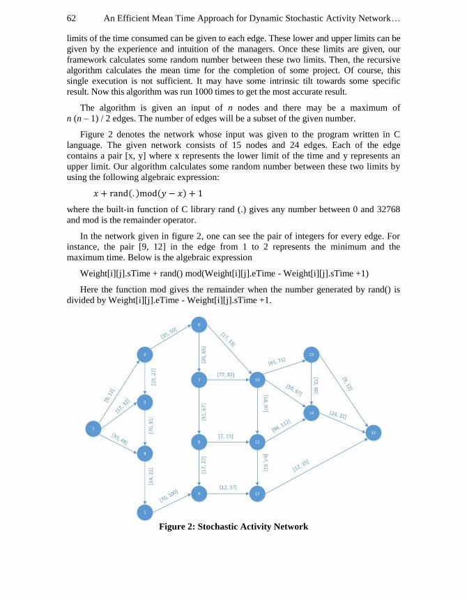
An Efficient Mean Time Approach for Dynamic Stochastic Activity Network… 62
limits of the time consumed can be given to each edge. These lower and upper limits can be
given by the experience and intuition of the managers. Once these limits are given, our
framework calculates some random number between these two limits. Then, the recursive
algorithm calculates the mean time for the completion of some project. Of course, this
single execution is not sufficient. It may have some intrinsic tilt towards some specific
result. Now this algorithm was run 1000 times to get the most accurate result.
The algorithm is given an input of n nodes and there may be a maximum of
n (n – 1) / 2 edges. The number of edges will be a subset of the given number.
Figure 2 denotes the network whose input was given to the program written in C
language. The given network consists of 15 nodes and 24 edges. Each of the edge
contains a pair [x, y] where x represents the lower limit of the time and y represents an
upper limit. Our algorithm calculates some random number between these two limits by
using the following algebraic expression:
( ) ( )
where the built-in function of C library rand (.) gives any number between 0 and 32768
and mod is the remainder operator.
In the network given in figure 2, one can see the pair of integers for every edge. For
instance, the pair [9, 12] in the edge from 1 to 2 represents the minimum and the
maximum time. Below is the algebraic expression
Weight[i][j].sTime + rand() mod(Weight[i][j].eTime - Weight[i][j].sTime +1)
Here the function mod gives the remainder when the number generated by rand() is
divided by Weight[i][j].eTime - Weight[i][j].sTime +1.
Figure 2: Stochastic Activity Network

Iqbal and Hasnain 63
Following is the corresponding node incidence matrix which models the given
network:
N =
[
]
---(2)
Following is the recursive algorithm that calculates the mean time for the completion
of all the activities:
MeanTime( integer NodeNumber)
1. k = 1; // this is the index for the columns of node-incidence matrix
2. l = 0; // this is the index for the predecessors to any node j
3. tMax = 0; // this is the initialization of the longest time of all paths to node j
4. while (l < numPredecessor(NodeNumber) )
5. if ( N[j, k] == -1)
6. i = 1;
7. while ( N[i, k] ≠ 1)
8. i++;
9. t = MeanTime (i) + Weight[i][j].sTime + rand() mod(Weight[i][j].eTime
- Weight[i][j].sTime
+1 );
10. if ( t >= tMax )
11. tMax = t;
12. l++;
13. k++;
14. return tMax;

An Efficient Mean Time Approach for Dynamic Stochastic Activity Network… 64
4. RESULTS
After simulating the program 1000 times, we got the results shown in the table 1
below. The more one simulates the program, the more better and refined results will
come out. This is the recurrent theme of the Monte Carlo simulation. The minimum taken
by our network during the simulation is 338 days whereas the maximum time taken by
the network is 449 days. The mean time calculated by the recursive algorithm is 395.42
days. This time is the result of the execution of the simulation for 1000 times as stated
earlier.
5. CONCLUSION AND FUTURE DIRECTIONS
In this paper, we used the Monte Carlo simulation for the calculation of the mean time
of the completion of a project. Although, the reported simulation has already been
successfully applied but it was plagued with the problem of some fixed network. The
main contribution of our paper is to tailor the recursive algorithm in such a way that it
could cope with network of any arbitrary size. In the previous work, we had to do the
drudgery of mathematical calculations, but through our contribution, it will remain no
longer. Our work can be extended if the probability of each path to be critical is also
calculated.
Table 1
Simulation Results
Sim
#
Mean
Time
Sim
#
Mean
Time
Sim
#
Mean
Time
Sim
#
Mean
Time
Sim
#
Mean
Time
Sim
#
Mean
Time
1 356.21 201 389.27 401 383.23 601 386.12 801 402.87 981 383.06
2 421.80 202 402.56 402 407.21 602 390.12 802 392.19 982 394.75
3 401.23 203 409.31 403 390.72 603 412.43 803 400.23 983 393.21
4 360.89 204 377.89 404 399.67 604 400.21 804 395.18 984 392.36
5 389.32 205 398.09 405 402.12 605 387.89 805 399.72 985 395.83
6 400.62 206 390.23 406 410.86 606 397.12 806 398.37 986 390.19
7 370.88 207 410.65 407 400.56 607 401.28 807 410.53 987 395.27
8 405.62 208 412.34 408 398.21 608 404.18 808 403.23 988 394.70
9 350.22 209 399.00 409 385.87 609 397.16 809 388.39 989 393.39
10 407.45 210 415.62 410 402.17 610 404.28 810 399.20 990 395.12
11 351.23 211 398.27 411 398.40 611 397.81 811 402.29 991 396.92
12 388.87 212 378.90 412 408.17 612 401.34 812 403.29 992 393.82
13 412.39 213 387.12 413 389.42 613 387.67 813 395.32 993 394.76
14 387.29 214 402.78 414 409.23 614 408.27 814 378.62 994 395.24
15 423.80 215 397.12 415 378.21 615 383.12 815 399.90 995 393.21
16 378.76 216 406.22 416 390.49 616 390.12 816 401.00 996 393.23
17 402.16 217 387.25 417 399.17 617 387.22 817 402.64 997 396.22
18 398.51 218 399.12 418 403.42 618 389.08 818 398.29 998 396.87
19 340.62 219 423.21 419 385.12 619 402.18 819 393.21 999 394.12
20 378.21 220 412.34 420 402.38 620 399.09 820 402.12 1000 395.42

Iqbal and Hasnain 65
REFERENCES
1. Avigad, J. (2010). Computers in Mathematical Inquiry. The Philosophy of
Mathematical Practice. https://doi.org/10.1093/acprof:oso/9780199296453.003.0012
2. Boyle, P. (1977). Options: a {M}onte {C}arlo approach. Journal of Financial
Economics, 4(3), 323-338. https://doi.org/10.1016/0304-405X(77)90005-8
3. Chapra, S.C. and Canale, R.P. (2015). Numerical methods for engineers. Mathematics
and Computers in Simulation, 33(3), 260.
https://doi.org/10.1016/0378-4754(91)90127-O
4. Cormen, T.H., Leiserson, C.E. and Rivest, R.L. (2001). Introduction to Algorithms,
Second Edition. Computer (Vol. 7). https://doi.org/10.2307/2583667
5. Glen, A.G., Evans, D.L. and Leemis, L.M. (2001). APPL: A probability programming
language. American Statistician (Vol. 8795).
https://doi.org/10.1198/000313001750358509
6. Homem-de-Mello, T. (2007). A study on the cross-entropy method for rare event
probability estimation. INFORMS Journal on Computing, 19(3), 381-394.
https://doi.org/10.1287/ijoc.1060.0176
7. Jäckel, P. (2002). Monte Carlo methods in finance. Book, (November), xvi, 222.
https://doi.org/10.1080/14697680400008601
8. Jing-Quan Li, P.B.M. and D.B. (2006). The k-Degree Cayley Graph and its
Topological Properties. Networks, 47(1), 26-36. https://doi.org/10.1002/net
9. Leemis, L. and Park, S. (2004). Discrete-Event Simulation : a First Course,
(December).
10. Park, S.K. and Miller, K.W. (1988). Random number generators: good ones are hard
to find. Communications of the ACM, 31(10), 1192-1201.
https://doi.org/10.1145/63039.63042
11. Sargent, R. (2005). Verification and validation of simulation models. Proceedings of
the 37th Conference on Winter Simulation, (mimic), 130-143.
https://doi.org/10.1109/WSC.2000.899697
12. Wilson, J.R. and Goldsman, D. (2001). Alan Pritsker's multifaceted career: theory,
practice, education, entrepreneurship, and service. Iie Transactions, 33(3), 139-147.

An Efficient Mean Time Approach for Dynamic Stochastic Activity Network… 66

67
Proc. ICCS-14, Multan, Pakistan
December 12-15, 2016, Vol. 30, pp. 67-78
REMOTE HOME TEMPERATURE CONTROL
USING IOT AND STOCHASTIC PROCESS
Nauman Shah, Farkhand Shakeel Mahmood and G.R. Pasha
National College of Business Administration and Economics
Multan, Pakistan
ABSTRACT
A luxurious, peaceful and comfortable home is the dream of every human being.
Humans struggle a lot to make their homes comfortable and more manageable. In doing
so, their prime priority is to set the home temperature that is more suitable for
comfortable living. Home temperature mostly depends upon the outside weather
conditions. Therefore, setting the suitable living temperature for the home each time
according to the weather conditions outside can be a hectic job for the home owner. On
top of all, once the temperature is set than owner will have to wait until the home
temperature changes from current temperature to desired one. This thing not only leads
towards the uncomfortable living environment plus it also adds some undesirable effects
on the owner’s mood.
To overcome all these hurdles an algorithm was designed and implemented. We
managed these devices from anywhere using our cellphone and saved the energy
consumed by these devices.
By means of Information Technology and Statistical Approaches like IoT (Internet of
Things) and Statistical Stochastic Process (Markov Chain) respectively, we managed the
home temperature efficiently and overcome expected problems. Temperature sensors
were used to sense the outside temperature conditions. Stochastic Processes controller
based on Markov Chain were designed to adjustment the home temperature w.r.t. outside
temperature conditions.
1. INTRODUCTION
There is no place like home in this world. Everybody struggles to make their home
more decorative, manageable, and comfortable. For that purpose they install different
electronic devices in their homes. These electronic devices can make the home look well
decorated and very comfortable. The most important device is the air-conditioner. Air
conditioners available today are used to control the temperature of the home according to
the single temperature value set by the owner/operator. Unfortunately, this thing seems
unrealistic and it is not understandable by most of owners. Because it is really difficult
for the owner to tell the exact temperature value that should suite his/her mood and
comfort level.
So, there should be a human friendly, easy to use, and personalized way for the home
owner to manage the temperature of his/her home according to his/her mood. On top of
all, air conditioners are heavy duty electronic devices and the cost of electricity is too

Remote Home Temperature Control using IoT and Stochastic Process 68
high now a day. Therefore there should also be a way to save the energy consumed by
these devices.
So, by using fuzzy logic a solution will be provided to the home owner that would
empower him to set the temperature of home by using easy to use and understandable
temperature benchmarks like: cold, warm, hot, very hot, cold, and very cold. Then, by the
use of IoT technology and Statistical Stochastic Process, the owner will be able to control
the home temperature by using his smart phone anywhere in the world.
2. RELATED WORK
The proposed research is based on two most widely used technologies those are
Fuzzy Logic and IoT. Fuzzy logic is an approach to computing based on "degrees of
truth" rather than the usual "true or false" (1 or 0) Boolean logic on which the modern
computer is based (“Fuzzy logic - Wikipedia,” 2016). A lot of work has done on fuzzy
logic. Fuzzy logic is designed and implemented in microcontroller without using any
special software tool (Hanamane et al., 2006). Different microprocessor based circuits
can be used to implement the Fuzzy Logic like 8085 based circuit (Hanamane et al.,
2006). The reason for using fuzzy logic in control applications stems from the idea of
modeling uncertainties in the knowledge of a system’s behavior through fuzzy sets and
rules that are vaguely or ambiguously specified (Aguilar et al., 2009). Fuzzy logic can
also be implemented by using Java language then it can be used in all the Java supported
hardware and microcontrollers (“jFuzzyLogic,” 2016). Arduino is Java based open-
source electronics hardware platform that supports the low cost and easy to use
implementation (Kumar et al., 2016). Arduino and Java technology can be used together
to create a low cost Fuzzy Logic controller with the support of IoT (He, 2016).
The IoT links objects to the Internet, enabling data and insights never available before
(“Internet of Things (IoT) - Cisco,” 2016). Internet of Things (IoT) is when the Internet
and networks expand to places such as manufacturing floors, energy grids, healthcare
facilities, and transportation (“Internet of Things (IoT) - Cisco,” 2016). By the use of IoT
and Arduino the home owner would be able to check the temperature and would be able
to manage the temperature of home regardless of time and place (Ra et al., 2016). The
main factor IoT concept is the integration of different technologies. The IoT is
empowered by the hottest developments in RFID, smart sensors, communication
technologies, and Internet protocols (Shah, 2016).
According to Hanamane, 2006 a hardware was developed which is used to control
temperature through fuzzy logic by ON-time of the heater through PPI 8255. The actual
temperature is read by the thermistor and it is compared with the temperature set by the
user. Microprocessor based control circuit is used to implement fuzzy controller.
Hasim, 2012 designed a fuzzy logic controller to control water bath temperature, it
will control temperature of water in real time, that means that the temperature of the
water will be controlled while bathing. It uses the MATLAB Fuzzy Logic Toolbox to get
the goal achieved. For designing of a fuzzy controller the 4x4 matrix rule is followed.
Yu, 2010 proposed a fuzzy rule based system that successfully incorporates the
flexibility of human decision making by means of the use of fuzzy set theory using

Shah, Mahmood and Pasha 69
algorithms and different linear programming techniques. Plus, an evolvable hardware is
also designed for making fuzzy controller more capable. The basic property of the
evolvable hardware is to dynamically change its architecture and behavior according to
the environment in which it is running.
To implement the automatic temperature setting in Textile Air Conditioning and
monitoring system on the basis of IoT, three subsystems were composed by H. Chen,
2015. These subsystems were: remote monitoring subsystem, database subsystem, and
local monitoring subsystem. The system uses GPRS communication and computer
networks to control the data both remotely and locally. The humidity and temperature
control has been done by the use of Fuzzy Controller.
Temperature control can be implemented in Green House by using adaptive method
based on fuzzy logic control (L. Chen et al, 2013). To get the greenhouse the exact and
desired temperature the mathematic model is constructed first. After that the MATLAB is
used with Simulink tools to implement the fuzzy logic controller. L. Chen, 2013 has
programmed the fuzzy controller by using the Visual Basic to control the greenhouse.
By the use of Arduino UNO a very low cost soil moisture check sensor can be
designed (Kumar et al., 2016). It is really difficult for the farmers to purchase the devices
to check the moisture level in the soil. The right moisture level in the soil guarantees the
higher crop yields. In case of inappropriate moisture level the system will guide the
farmer to give or stop the water supply to the crops.
A lot of work has been done on food monitoring during cooking and packing. But, for
monitoring the quality of the food while transporting the food to different
locations/destinations there is a need for some improvement in the standards.
Maksimović, Vujović et al., 2015 has ensured the monitoring of the food safety and
traceability while transportation of the food from one place to another. This is a low cost
IoT solution that helps the managers to have an eye on the food even when it is being
transported to some other location all the way.
IoT is being used most widely in home automation and in creating smart buildings.
Different protocols are used in home automation, like: ZigBee, Wi-Fi, and Bluetooth. The
problem is that the existing home equipment often require network communication
enabled power plugs or devices. These devices use some unique communication protocol
defined by the company. Therefore these devices are not able to communicate with other
devices. In Ra et al., 2016, has solved this problem by using Smart Home Automation
Framework (SHAF). Here Ruspberry Pi and ZigBee is used as the smart home server.
Client is the android and windows smartphone.
In IoT the network and sensor performance is a really very critical thing. Network
components and sensors works as the integral part of IoT. By using the soft computing
technologies like Fuzzy Logic the performance of network and sensors can be improved a
lot. Maksimović at al., 2015 used the soft computing technologies for the detection and
monitoring of the residential based fire is being done very efficiently.
Internet of things defines the worldwide network of smart objects those can
communicate with each other on the computer network and get the information on the
basis of the sensors attached with them. This information can be accessed anywhere in

Remote Home Temperature Control using IoT and Stochastic Process 70
the world by the use of computer networks. These objects keeps on interacting with each
other and it requires more power. The more these sensors are efficient the less power they
will consume. Choice of the algorithms to program these objects also plays an important
role in power/energy consumption. Vujovic et al., 2015 designed a prototype sensor node
with fuzzy logic for decision making process is built and tested in real time.
Singhala et al., 2014 proposed a room temperature controller designed by using fuzzy
logic controller. Here the first job of temperature control is to set the temperature up to
the required temperature and second job of temperature control is to insure that the
temperate is according to the desired value. The desired output is get by using the
feedback controller. MATLAB is used here to design the Fuzzy Controller.
The short fuzzy logic tutorial is designed by Yildiz, 2010 that helps the starters to
design the fuzzy logic controller. It explains that the crisp inputs are taken and then it is
converted to the fuzzy set using the fuzzy linguistic variables, terms and member
functions. This thing is called fuzzification (Yildiz, 2010). Than on the basis of rules
inference is made. In the end by the use of defuzzification process the fuzzy output is
mapped to the crisp output. It also identifies the way to control the temperature of the air
conditioner.
Fuzzy logic technique is used to design the solution for multi-parameter and non-
linear control model (Isizoh et al., 2012). It makes the solutions efficient than the
traditional control design techniques. Here microcontroller, temperature sensor, and the
operational amplifier, analogue to digital converter, display and output interface circuit
are used to design the fuzzy logic based temperature control system.
Yao et al., 2015 stated that the buildings in United States consume 74% of electricity
of the country. The number of energy efficient buildings is very less and their
performance is unsatisfactory. Therefore there is a huge loss due to this huge electricity
consumption. Plus the emission of greenhouse gases is resulting in the more polluted
environment. Yao, 2015 offers to increase the efficiency and effectiveness of the
buildings by installing smart building IoT features and putting them on to the solar
power. As, at the day time the building will get the energy form the Sun and will also
store that energy in the battery so that that energy could be consumed later on. And when
the day light begins to wash away, the buildings are converted automatically to the
battery source those were charged all day long, as at night the consumption of the
electricity is lower comparing to the consumption of electricity at day time.
3. STOCHASTIC PROCESS
Stochastic process is statistical model which deals with random variable. In this
process the changings in a system depend on the random variable which is taken as input
and given as output. The initial state in stochastic process is important because depending
on this state many other states can be derived. Next states in a system can be derived
through prior and current state. Stochastic process can be used widely in different fields
for verifying results of data for example in stock exchange, signals such as speech audio
and video, medical data like blood pressure and temperature control.

Shah, Mahmood and Pasha 71
Markov Chain or Markoff Chain
is a probabilistic process which
satisfies Markov property. Basic
statement of Markov chain is if one
can have the knowledge about the
current status of the system than by
this only piece of information we can
predict the future of the system.
Because of these special features
of stochastic process we are using
this approach in our system for
controlling temperature and adjusting
it accordingly.
4. FUZZY CONTROLLER
Fuzzy Controller is a system in which
fuzzy logic is implemented for calculating
the results. Fuzzy controller is built after
following some major principles
described below.
4.1 Fuzzification
Input variables of fuzzy system are
mapped by sets of membership functions
known as fuzzy sets. In our system the
fuzzy sets related to temperature are too-
cold, cold, warm, Hot, too-hot. Fuzzy sets
and fuzzy membership functions are two
important points to understand. As we
have set 40°C<TEMP<80°C then if
temperature is 40 it did not belong to hot
but in fuzzy set it belong to hot with 0
membership function. And if temperature
rises like 60°C<TEMP<80°C then
membership function will be 0.98. The
crisp input values are converted into
fuzzy values and this process of
conversion is called fuzzification.
Fig 1: Stochastic Process Controller
Fig 2: Fuzzy Logic System
Start
Input
Convert input to Fuzzy Set using MFs and Linguistic Vars
Draw Inference on Rules Basis
Convert fuzzy output using MFs
Output
End

Remote Home Temperature Control using IoT and Stochastic Process 72
4.2 Membership Functions:
Membership functions is curve built in MATLAB and are used to mapped
membership values between 0 and 1. They actually show how input space is mapped to
membership value. Membership function for inside temperature, outside temperature and
set temperature are given below.
4.2.1 Inside Temperature Membership Function:
We will give inside temperature as input variable. The figure shows that temperature
less than 24°C will be cold and temperature between 24°C and 26°C is warm and above
that will be hot.
Fig 3: Inside Temperature
4.2.2 Outside Temperature Membership Function:
We will give outside temperature as output variable. The figure shows that
temperature less than 24°C will be cold and after that variability in temperature is shown.
Fig 4: Outside Temperature

Shah, Mahmood and Pasha 73
4.2.3 Set Temperature Membership Function:
If temperature is given in between 0°C and 24°C then hot air will be set and if
temperature is greater than 26°C then cold air will be set.
Fig 5: Set Temperature
4.3 Fuzzy Rules
Fuzzy rules are implemented by using simple IF ELSE logic. These rules are used for
controlling the output variable. The heating and cooling will be turned on by the
Temperature Controller on the basis of inside home temperature.
Fig 6: Fuzzy Rules for Setting Temperature
A graph is also drawn in MATLAB for clearing fuzzy rules.

Remote Home Temperature Control using IoT and Stochastic Process 74
Fig 7: Fuzzy Rules Graph
4.4 Inference
Fuzzy Inference involves membership functions, fuzzy rules and logical operators.
Mapping from given input to an output using fuzzy logic is fuzzy inference. This diagram
is showing the surface view and inference of fuzzy system.
Fig 8: Surface View of Temperature Control System
4.5 Defuzzification
Combining all result and given a single output is called defuzzification.
5. IMPLEMENTATION OF WORK
The system will take two inputs by the use of temperature sensor TMP-36. One
temperature sensor will be placed outside to monitor the outside temperature and one
temperature sensor will be placed inside the room to sense the temperature of the room.
Both temperature sensors will send the inputs to the following two components:
1. Fuzzy Controller
2. IoT Controller (Arduino Ethernet Shield)

Shah, Mahmood and Pasha 75
Fig 9: Structure of Proposed Temperature Control System
The fuzzy controller will convert both of the input temperatures to the user
understandable output by using the linguistic variables and member functions.
Temperatures will be converted to either Very Cold, Cold, Warm, Hot, and Very Hot.
After converting the temperatures the fuzzy controller will choose and suggest the output
temperature that would be most appropriate for the home. Fuzzy controller will send that
temperature to the Stochastic Controller.
Stochastic Controller is attached directly with the home appliances (Fan, Heater, and
Air Conditioner) and it is responsible for controlling these devices on the basis of the
output gained from the Fuzzy Controller. Stochastic Controller is implemented by using
Markov Chains.
Fig 10: Implementation of the Fuzzy/Stochastic Temperature Controller

Remote Home Temperature Control using IoT and Stochastic Process 76
The stochastic controller, located inside the room, will adjust the most feasible and
comfortable room/home temperature according to the states defined in the Markov Curve.
The following states are defined in our Stochastic Controller:
1. Turn ON Heating Air
2. Turn OFF Heating Hair
3. Turn ON Cool Air
4. Turn OFF Cool Air
5. Turn ON Fan/Exhaust
6. Turn OFF Fan/Exhaust
All the room temperature controllers and devices do not consider the outside
temperature to control the home temperature. Here the point is: if because of just turning
on the exhaust the home environment can be made more feasible for living than why
there is a need to turn on the heating and cooling to make room temperature stable? And
surely this saves a lot of energy consumption. So, the Stochastic Controller will keep on
switching the Fan/Exhaust if the fuzzy controller believes that the temperature can be
maintained by just using the exhaust. This thing will make the home environment natural
and will also reduce the energy consumption.
Both of the controllers in our system are connected to the Arduino Ethernet Shield
that is connected to the internet and publishing the statuses of the Stochastic Controller
and temperature conditions of the inside and outside temperatures. By the use of Arduino
and Ethernet shield we have made it possible for our Temperature Controller to enable
the Internet of Things (IoT) technology. Because of this the current temperature of the
home and outside can be checked no matter wherever the home owner is. Second, the
working and performance of the Air Conditioning devices is also accessible regardless of
the location.
6. CONCLUSION
In the Temperature Controlling Systems available today, there is not any option to
control the home temperature on the basis of the outside weather. Our temperature
controller, by the use of Fuzzy Logic, Markov Chain, and IoT techniques makes it
possible to design an efficient and power saving air conditioning controller device. Fuzzy
Controller is designed for managing home temperature. The theme is to use the fresh air
if it is feasible to change the home temperature. Simulations and testing have been shown
in paper which is done in MATLAB. Stochastic process controller is setting temperature
of inside according to outside weather. Through practical implementations of fuzzy
controller and stochastic process controller it is seen that with affordable budget we can
design an efficient and power efficient system that is also compatible with IoT
technology.

Shah, Mahmood and Pasha 77
REFERENCES
1. Aguilar, R. M., Muñoz, V. and Callero, Y. (2012). Control application using fuzzy
logic: Design of a fuzzy temperature controller. INTECH Open Access Publisher.
2. Chen, H. (2015). Implementation of Textile Air Conditioning Intelligent Monitoring
System Based on Internet of Things. International Journal of Smart Home, 9(12),
267-278.
3. Chen, L., Zhang, H. and Du, S. (2013). Greenhouse Temperature Control System
Based on Fuzzy Theory. 2013 Third International Conference on Instrumentation,
Measurement, Computer, Communication and Control, 1673-1677.
http://doi.org/10.1109/IMCCC.2013.370
4. Wikipedia (2016). Fuzzy logic. Retrived on October 10, 2016 from
https://en.wikipedia.org/wiki/Fuzzy_logic
5. Hanamane, M.D., Mudholkar, R.R., Jadhav, B.T. and Sawant, S.R. (2006).
Implementation of fuzzy temperature control using microprocessor. Journal of
Scientific & Industrial Research, 65, 142-147.
6. Hasim, N., Aras, M. S. M., Ab Rashid, M.Z., Kassim, A.M. and Abdullah, S.S.
(2012). Development of fuzzy logic water bath temperature controller using
MATLAB. In IEEE International Conference on Control System, Computing and
Engineering (ICCSCE), (pp. 11-16).
7. He, J., Atabekov, A., & Haddad, H. M. (2016, August). Internet-of-Things Based
Smart Resource Management System: A Case Study Intelligent Chair System.
In 25th
International Conference on Computer Communication and Networks
(ICCCN), (pp. 1-6).
8. Internet of Things (IoT)-Cisco. (2016). Retrieved on October 10, 2016, from
www.cisco.com/c/en/us/solutions/internet-of-things/overview.html
9. Isizoh, A.N., Okide, S., Anazia, A. and Ogu, C. (2012). Temperature Control System
Using Fuzzy Logic Technique. International Journal, 1(3), 27-31.
10. Fuzzy Logic (2016). Retrieved on January 1, 2016, from jfuzzylogic.sourceforge.net
11. Kumar, M.S., Chandra, T.R., Kumar, D.P. and Manikandan, M.S. (2016). Monitoring
moisture of soil using low cost homemade Soil Moisture Sensor and Arduino UNO,
4-7.
12. Kumar, M.S., Chandra, T.R., Kumar, D.P. and Manikandan, M.S. (2016). Monitoring
moisture of soil using low cost homemade Soil moisture sensor and Arduino UNO. In 3rd International Conference on Advanced Computing and Communication Systems
(ICACCS), 1, 1-4.
13. Maksimović, M., Vujović, V. and Omanović-Mikličanin, E. (2015). A low cost
internet of things solution for traceability and monitoring food safety during
transportation. CEUR Workshop Proceedings, 1498, 583-593.
14. Maksimović, M., Vujović, V., Perišić, B. and Milošević, V. (2015). Developing a
fuzzy logic based system for monitoring and early detection of residential fire based
on thermistor sensors. Computer Science and Information Systems, 12(1), 63-89.
15. Ra, H. K., Jeong, S., Yoon, H. J., & Son, S. H. (2016, August). SHAF: Framework for
Smart Home Sensing and Actuation. In 22nd
International Conference on Embedded
and Real-Time Computing Systems and Applications (RTCSA), 258-258.
16. Shah, S.H. (2016). A Survey : Internet of Things ( IOT ) Technologies , Applications
and Challenges, i, 381-385.

Remote Home Temperature Control using IoT and Stochastic Process 78
17. Shah, S.H. and Yaqoob, I. (2016). A survey: Internet of Things (IOT) technologies,
applications and challenges. In Smart Energy Grid Engineering (SEGE), 381-385.
18. Singhala, P., Shah, D.N. and Patel, B. (2014). Temperature Control using Fuzzy
Logic. International Journal of Instrumentation and Control Systems (IJICS), 4(1),
1-10.
19. Vujovic, V., Jokic, S. and Maksimovic, M. (2015). Power Efficiency analysis in
Internet of Things Sensor nodes. In Proceedings of the 2nd Int. Electron. Conf. Sens.
Appl., Sciforum Electronic Conference Series, Vol. 2, 2015, D005.
20. Yao, L., Lai, C.C. and Lim, W.H. (2015). Home Energy Management System Based
on Photovoltaic System. 2015 IEEE International Conference on Data Science and
Data Intensive Systems, 644-650.
21. Yildiz, Z.C. (2010). A Short Fuzzy Logic Tutorial, (Figure 2), 1-6. Retrieved from
http://cs.bilkent.edu.tr/~zeynep/files/short_fuzzy_logic_tutorial.pdf
22. Yu, H. (2010). Design of Fuzzy Logic Controllers Based on Evolvable Hardware
Platform. 2010 Fourth International Conference on Genetic and Evolutionary
Computing, 2, 864-867.

79
Proc. ICCS-14, Multan, Pakistan
December 12-15, 2016, Vol. 30, pp. 79-89
F.I.R. OF DIABETES EMPLOYING FUZZY LOGIC
IN ANDROID OPERATING SYSTEM
Ali Raza, Farkhand Shakeel Mahmood and Moizu Din
National College of Business Administration and Economics, Multan, Pakistan
Email: [email protected] and [email protected]
ABSTRACT
In the past, diagnosis of a disease was done by medical experts. Then computer came
and some medical decision support system (MDSS) were introduced to accomplish the
task. Now a days, computers are being replaced by portable devices including cell phones
and tablets gradually. These devices use Android and iOS as their operating systems. In
such circumstances, an application of MDSS is required that can give first information
report (FIR) about a disease to a person without going to a doctor.
In this work, we focused on diabetes. Non pathological data of a person and standards
of World Health Organization (W.H.O) were used to get FIR. Different fuzzy rules were
made to design an inference engine. It was developed in Android framework. This work
fulfills the need of MDSS and gives FIR to a lay person about his diabetic condition at
any time and any place.
KEY WORDS
Diabetes, Fuzzy Logic, Android, iOS, MDSS, Non-pathological.
1. INTRODUCTION
Information is very important and vital part of this world. It makes us to be civilized
and have a better power of decision. It also plays a fundamental role in the progress of
this world. In the light of information, we can make our lives better, prosper and healthy.
That's the reason that peoples or researchers have a race to get more information and facts
and spread it out to the other peoples to make their lives better.
Today, technology is going to be common and affordable to almost every person.
Spread of this technology has adverse effect on our life style. That's why human becomes
the victim of different chronic diseases specially Diabetes Mellitus. According to World
Health Organization (W.H.O), 194 million peoples in this world are suffering from this
disease. According to a prediction of W.H.O, the number of diabetic patients can be
increased up to 300 million in 2025. This number is alarming situation for this world. To
control this number, we will have to predict or detect their diabetes at early stage.
Now a days, mobile technology has a great progress and is using by almost every
person of this world. Android phones also become a part of people's life. By using the
apps of this android phones, we can make our lives easy and better. This work is also an
effort to detect Diabetes Mellitus at its early stage and give the suggestion to patients to
visit doctor for further treatment and pathological tests.

F.I.R. of diabetes Employing Fuzzy Logic in Android Operating System 80
A lot of work has been done by many researchers in Diabetes Detection. But I used
fuzzy logic for this purpose. Although a lot of work is done in this field. But the specialty
of this work is the use of non pathological data, android technology and fuzzy set
operators. A new algorithm is also designed. This algorithm will take five inputs from the
users. After getting input, it will process these inputs by using fuzzy logic. In processing,
different fuzzy operators will be implemented and then defuzzify it.
1.1 Purpose of this Work The purpose of this work is to inform the peoples about the initial status of their
diabetic condition. Following persons can get benefit from the purposed system:-
Everyone who is health conscious
The persons who are so busy in their daily life
The persons who are in remote areas
1.2 Assumptions: m kj
1. Only adults are focused in this research
2. Normal person are considered. Lactating or Pregnant women are not considered in
this research
3. All the data is based upon the normal conditions e.g. normal temperature or normal
life style of a person
2. LITERATURE REVIEW
A plenty of work has been done on fuzzy logic, medical diagnosis, android operating
systems and diabetes detection. Many books and research articles of these field are also
published.
Zadeh [15] introduced the fuzzy logic in 1964. In his work, he purposed the degree of
vagueness in the contrast of traditional logic crisp where completely true and completely
false were considered.
Kosko [6] discussed the past, present and future of fuzzy logic. The author described
the fuzzy principal that everything in fuzzy is a matter of degree.
Wiriyasuttiwong and Narkbuakaew [14] purposed a medical knowledge base system
(MKBS) for diagnosis from symptoms and signs. It was made to support medical
knowledge construction about a disease based on production rules.
Licata [7] described a clinical case in the light of fuzzy logic. An inference engine for
a person suffering from many diseases was developed and showed that fuzzy logic is
much better than probabilistic analysis.
Balanacia et al. [2] discussed about the correct diagnosis and assessment of Breast
cancer Risk. Different fuzzy variables were discussed under fuzzy rules and risk factor of
Breast Cancer was also determined.
Soundararajan et al. [11] developed a decision support system based on fuzzy logic to
detect Tuberculosis. Work on detecting the risk of tuberculosis was also done in this
paper. The algorithm defined in this paper was based on fuzzy rules.

Raza, Mahmood and Moizu Din 81
Pervin and Abhari [9] worked on Fuzzy Database for Heart Disease Diagnosis. An
algorithm was developed based on different fuzzy variables and heart condition was
calculated here.
Efosa et al. [4] worked on diagnosis and therapy of HIV/AIDS. For diagnosis and
therapy of these diseases, Fuzzy logic and data mining approaches were used.
Margret et al. [8] worked on the design of a Diabetic Diagnosis System. For this
purpose, simple Rough Sets in symptoms were used. An algorithm is also designed and
system is implemented to diagnose diabetes.
Bodhe et al. [3] purposed a Health Care System. In their work, patient diagnostic
system was purposed by using android operating system. They used client server model
for communication with the users. Their purposed system tells about the degree of
severity of illness.
Sreedevi et al. [13] introduced a model of Diabetes diagnosis. In their work, a
Threshold Genetic Algorithm was used for Diagnosis of Diabetes using Minkowski
Distance Method.
Giri and Todmal [4] worked on diabetes prediction. For this purpose, they used
Neural Network, Fuzzy Logic and Gaussian Kernel Method in Prognosis of Diabetes.
Akter and Shorif [1] developed a new database management system with user friendly
interface. They used android operating system for this purpose.
Sonawane and Patil [13] made a system for prediabetic patients. They used genetic
programming to detect the pre diabetes. The purposed system worked in two portions i.e.
one for training data and second one was for classification of the available features.
Jain and Raheja [9] worked for improving the Prediction Rate of Diabetes using
Fuzzy Expert System. They first convert the experimental data set into crisp values and
then from crisp into fuzzy values. The system provides knowledge about diabetes after
fuzzification by applying different rules.
3. PURPOSED SYSTEM
Fig. 1: Inference Engine

F.I.R. of diabetes Employing Fuzzy Logic in Android Operating System 82
Plenty of work is done on medical diagnosis. Different applications are also made by
different developers. But they mostly used pathological calculations. In this work, we
only used early symptoms of different risk factors. No pathological values are used here.
Methodology used in the this algorithm is Fuzzy Logic. Here we used different ranges of
a fuzzy variables. Different fuzzy rules and defuzzification are also the part of this
inference engine i.e. Matlab is used to handle these fuzzy ranges and their linguistic
variables. In Matlab following variables with their ranges are defined:-
3.1 Variables In the above defined inference engine, we have following fuzzy variables with ranges
of their values.
i) Input Variable 1
Water_Intake_Glasses with member function (Below, Normal, High and Very High).
Range of Fuzzy Values that are Defined Over this Variable is given below in the
Table.
Table 1
S# Input Field Name Values Range Fuzzy Linguistic Variable
1 Water_Intake_Glasses
< 5 Below
5-11 Normal
12-15 High
> 15 Very High
Fig. 2: Member Ship Function for input variable (Water_Intake_Glasses)
ii) Input Variable 2
Urination Times with member function (Below, Normal, High and Very High) Range
of fuzzy values that are defined over this variable is given below in the table:

Raza, Mahmood and Moizu Din 83
Table 2
S# Input Field Name Values Range Fuzzy Linguistic Variable
2 Urination Times
<4 Below
4-9 Normal
10-14 High
>14 Very High
Fig. 3: Member Ship Function for Input Variable (Urination Times)
iii) Input Variable 3
Unexpected Weight Loss Kg with member function (Ignore, Normal, High and Very
High). Range of fuzzy values that are defined over this variable is given below in the
Table.
Table 3
S# Input Field Name Values Range Fuzzy Linguistic Variable
3 Unexpected Weight
Loss Kg
<2 Ignore
2-4.5 Normal
5-8 High
>8 Very High
Fig. 4: Membership Function for Input Variable (Unexpected Weight Loss kg)

F.I.R. of diabetes Employing Fuzzy Logic in Android Operating System 84
iv) Input Variable 4
Cuts Wounds Healing Time Days with member function (Early, Normal, Late and
Very Late). Range of fuzzy values that are defined over this variable is given below in
the Table.
Table 4
S# Input Field Name Values Range Fuzzy Linguistic Variable
4 Cuts Wounds Healing
Time Days
<5 Early
5-12 Normal
13-18 Late
>18 Very Late
Fig. 5: Member Ship Function for input variable (Cuts Wounds Healing Time Days)
v) Input Variable 5 Hunger with member function (Low, Normal, Sharpe and Extreme). Range of fuzzy
values that are defined over this variable is given below in the Table.
Table 5
S# Input Field Name Values Range Fuzzy Linguistic Variable
5 Hunger Insensitivity
1 Low
2 Normal
3 Sharpe
4 Extreme

Raza, Mahmood and Moizu Din 85
Fig. 6: Member Ship Function for input variable (Hunger Intensitivity)
vi) Output Variable 6
Prediabetic Condition with member function (Healthy, At Risk and Prediabetic).
Prediabetic are the patients who have glucose level above the normal but below the
diabetic condition. Range of fuzzy values that are defined over this variable is given
below in the graph:
Fig. 7: Member Ship Function for output variable (Prediabetic Condition)
This output is calculated with some fuzzy rules. These rules contain 5 variables with
different intensive value ranges. These rules with different variables and algorithm are
given in the Table 6.
3.2 Algorithm
Each variable Range has 20% contribution in prediabetic situation. These ranges are
defuzzified and produces output in the form of crisp logic i.e.0 or 1. The criteria of output
is if the input of 2 variables belong to two upper classes, then there is "Healthy" is
selected as outcome. While if value of 3 variables belongs to two upper classes, then it
will produce "At Risk" and if the value of 4 or 5 variables belong to two upper classes,
then it will show "Prediabetic".

F.I.R. of diabetes Employing Fuzzy Logic in Android Operating System 86
Table 6
S# Detail Description
1 Input
Variables
1. Water_Intake_Glasseds
2. Urination_Times
3. Unexpected_Wright_Loss_kg
4. Cut_Wounds_Healing_Times_Days
5. Hunger_Insensitivity
2 Output
Variables
1. Healthy
2. At_Risk_being_Prediabetic
3. Prediabetic
3 Methodology Fuzzy logic with linguistic variables having
ranges expressed in member functions
4 Algorithm
Button_Click()
Start Integer Risk factor=0
if (Water_Intake_Glasseds is equal to
"High" OR "Very High" )
Risk factor=Risk factor+2;
if (Urination_Times is equal to "High"
OR "Very High" )
Risk factor=Risk factor+2;
if (Unexpected_Wright_Loss_kg is
equal to "High" OR "Very High" )
Risk factor=Risk factor+2;
if (Cut_Wounds_Healing_Times_Days is
equal to "Late" OR "Very Late" )
Risk factor=Risk factor+2;
if (Hunger_Insensitivity is equal to
"Sharpe" OR "Extreme" )
Risk factor=Risk factor+2;
if (Risk factor<5)
Display Toast "You are Healthy"
else if (Risk factor<7)
Display Toast "You have a risk
of being Pre-Diabetic"
else if (Risk factor>7)
Display Toast "You are Pre-
Diabetic.
Plz go to
doctor for further proceedings."
End

Raza, Mahmood and Moizu Din 87
For this purpose, different fuzzy rules are defined. Some of them are given below:-
3.3 Purposed System Implementation:-
A system was also developed in java by using android studio (2.1.3v). The snapshots
of the different states of developed system are given below:
5554:Nexus_5X_API_23 5554:Nexus_5X_API_23
Fig. 10: Initial State of the System Fig. 11: Healthy State
5554:Nexus_5X_API_23 5554:Nexus_5X_API_23
Fig. 12: Risk of being Prediabetic State Fig. 13: Prediabetic State

F.I.R. of diabetes Employing Fuzzy Logic in Android Operating System 88
3.4. Result and Discussion The developed system was tested on different peoples including normal and diabetic
patients. They used the application and gave good response in the sense of satisfaction.
More than 98% peoples seemed to accept the result and were satisfied. Following table
shows the result of testing.
Table 7
Total Persons Healthy At Risk Prediabetic
237 95 40 102
4. CONCLUSION AND FUTURE WORK
In this work, an android base system is defined with the help of Matlab fuzzy tool. In
this system, we used 5 risk factors including urine, thirst, Cuts and Wound Healing Time,
Hunger and Un expected Weight Loss of diabetes. Here we defined some fuzzy values,
then we made inference engine with some rules. Then we defuzzified the variable values
and make the crisp logic from these fuzzy variables.
The case study that we choose for this paper is diabetes. This work only tells that
either one is pre diabetic or not. My next Plan is to include pathological data and make it
more useful for medical practitioners.
There is also a plan that same technique will also be applied to detect Heart diseases
in further work. Medicines prescription can also be added in this work as future
enhancement.
REFERENCES
1. Akter, M., and Uddin, M.S. (2015). Android-based Diabetes Management
System. International Journal of Computer Applications, 110(10), 5-9.
2. Balanică, V., Dumitrache, I., Caramihai, M., Rae, W. and Herbst, C. (2011).
Evaluation of breast cancer risk by using fuzzy logic. University Politehnica of
Bucharest Scientific Bulletin, Series C, 73(1), 53-64.
3. Bodhe, M.K.D., Sawant, R.R. and Kazi, M.A. (2014). A Proposed Mobile Based
Health Care System for Patient Diagnosis using Android OS. International Journal of
Computer Science and Mobile Computing, 3(5), 422-427.
4. Efosa, C.E., Akinyokun, O.C. and Olatubosun, O. (2013). Online Fuzzy Logic
Knowledge Warehousing and Mining Model for the Diagnosis and Therapy of
HIV/AIDS. International Journal of Computational Science and Information
Technology, 1, 27-40.
5. Giri, T.N. and Todmal, S.R. (2015). Prognosis of diabetes using neural network,
fuzzy logic, gaussian kernel method. International Journal of Computer
Applications, 124(10), 33-36.
7. Jain, V., & Raheja, S. (2015). Improving the Prediction Rate of Diabetes using Fuzzy
Expert System. International Journal of Information Technology and Computer
Science (IJITCS), 7(10), 84-91.
6. Kosko, B. (1993). Fuzzy Thinking, Re-Print Edition, New York: Hyperion.

Raza, Mahmood and Moizu Din 89
8. Licata, G. (2010). Employing Fuzzy Logic in the Diagnosis of a Clinical Case.
Health, 2, 211-224.
9. Margret, A.S., Clara, L.J., Jeevitha, P. and Nandhini, R.T. (2013). Design of a
diabetic diagnosis system using rough sets. Cybernetics and Information
Technologies, 13, 124-139.
10. Parvin, R. and Abhari, A. (2012). Fuzzy database for heart disease diagnosis. In The
Proceedings of Medical Processes Modeling and Simulation (MPMS) of the 2012
Autumn Simulation Multi-Conference (SCS/AutumnSim'12.
11. Sonawane, R. and Patil, S. (2015). Diabetes Detection using Genetic Programming.
International Journal of Computer Applications, 127, 12-16.
12. Soundararajan, K., Sureshkumar, S. and Anusuya, C. (2012). Diagnostics Decision
Support System for Tuberculosis using Fuzzy Logic. International Journal of
Computer Science and Information Technology & Security, 2, 684-689.
13. Sreedevi E. and Padmavathamma M.,(2015), A Threshold Genetic Algorithm for
Diagnosis of Diabetes using Minkowski Distance Method. International Journal of
Innovative Research in Science, Engineering and Technology, 4, 5596-5601.
14. Wiriyasuttiwong W. and Narkbuakaew W. (2009). Medical Knowledge-Based
System for Diagnosis from Symptoms and Signs, International Journal of Applied
Biomedical Engineering, 2, 54-59.
15. Zadeh L.A. (1965). Fuzzy sets. Information and Control, 8(3), 338-353.

F.I.R. of diabetes Employing Fuzzy Logic in Android Operating System 90

91
Proc. ICCS-14, Multan, Pakistan December 12-15, 2016, Vol. 30, pp. 91-103
EXPLORING FEASIBILITY OF INTERFACE FOR COMMON
COMPUTER APPLICATIONS FOR ILLITERATE USERS
Syed Saqib Raza Rizvi
National College of Business Administration and Economics, Lahore, Pakistan
Email: [email protected]
ABSTRACT
Eight hundred million people in the world are illiterate they not only resides in
developing countries, this is a matter of concern that 43% of United Sates population is
functionally Illiterate. They are excluded from the benefits which computers provides
because there illiteracy is the biggest hurdle for understanding and taking advantages
from these modern and complex machines. To empower everyone and make computer
more accessible for this type of user group we designed and evaluated a prototype of
interface for common computer applications. To reach final prototype our early designed
prototype which will be based on the illiterate users need and mental model would be
refined over two usability iterations. Before starting the studies we well understood
design needs for illiterate and low literacy population from prior studies. We also
explored the understanding and special needs of illiterate users, we further discussed
some software design recommendations for software designers and developers.
GENERAL TERMS
User Interface, Design.
KEYWORDS
Illiterate, User Interface, Design, Human Factors.
1. INTRODUCTION
U.N. defines an illiterate person as someone who can “…with understanding both
read write a short simple statements in his or her everyday life” (Frisca 2012). Around
800 million people in the world are illiterate (Dew 2013; Frisca 2012; Knoche 2012) that
mean they don’t even know how to read or write simple sentences even using their
mother tongue. Illiterate population not only reside in developing countries, even
developed countries like U.S.A has 43% of population which is functionally illiterate
(Choudry 2012; Knoche 2012). Low literacy and low education are linked to other
disadvantages like poverty, unemployment and low-socioeconomic status (Choudry
2012; Medhi 2009).
To empower illiterate community world-wide so that they could also take advantage
from modern day technologies. A computer based application has been developed which
is providing an interface for common computing applications. In the recent past, many
studies have been conducted to empower illiterate and semi-illiterate users worldwide but

Exploring Feasibility of Interface for Common Computer Applications… 92
most of the research work has focused mobile applications. Studies have shown that
people with low literacy skills find mobile phones easy to operate and learn rather the
desktop computers (Chaudry 2012), but this study was conducted in year 2007 mobile
phones at that time were not as complicated as today, more over many American adults
with low-income access internet from there smart phones rather than computers (Chaudry
2012). Also the increase in mobile subscription, which was estimated 91.8% and 73.5%
inhabitants of developing countries and even in Africa respectively (Belay 2016).
Emergence of new manufacturers also increased availability of smart phones and there
market cost is less than 100 USD also mobile phones consumes very less power than
computers to work and energy is one of the most biggest problem in developing regions
like Africa (Agarwal 2013) and Asia. The rate of mobile phone usage is increasing even
in poor community (Medhi 2009). After all studies and researches still usability remains a
major hurdle for illiterate and semi-illiterate population (Medhi 2011; Mahmood 2014).
For designing our application we had used computers instead of smartphone for
different reasons. Our application contains different multimedia supported features which
include video and audio help support for the user which slightly increased the size of our
designed application, limited memory, space and less hardware capabilities of mobile
phones were not able to run our application properly (Belay 2016). If we put all the
support features online it would had brought difficulty to our users because of high cost
and minimum coverage of wireless internet world-wide. Another reason for developing
computer application instead of mobile is cost, in developing countries smartphones with
greater hardware specifications and software capabilities are still expensive roughly
estimated cost above 100 USD (Agarwal 2013; Frisca 2012), but a desktop computer
with above average hardware capabilities is not more than 60 USD. Moreover Chipchase
et al. argued in against of making smartphones and applications for illiterate users which
were visible and recognizable by others because it can stigmatize a user (Knoche 2012),
therefore Kristin et al. proposed system was based upon values-sensitive design (Dew
2013) to avoid stigmatic issues, this is also another very important reason to design
computer based application rather than mobile based.
The goal of this paper is to explore the feasibility of our application, which contains
interface for common usable computer applications, our goal is to make this computer
based application accessible for population with less to no literacy. We adapted User
Centered design policy, we designed and built the application totally according to user’s
needs and capabilities which we understood during our study. We had also discussed
some user interface design recommendations for illiterate and semi-illiterate population
latter on.
We conducted our study in three phases. In the first phase we interviewed illiterate
people and tried to find their needs and explored there understanding about computers to
understand user’s mental model, and from the information obtained from the first phase
we developed first prototype. In second phase of our study we trained the participant
about how to use the application, we also noticed the difficulties and coping strategies
which they used for performing different tasks which were given to them. We also noted
there suggestions regarding to the user interface, in short in the second phase participants
performed usability testing. In the third phase of our study we developed a refined
prototype based on the observation and recommendations given by our participants in

Syed Saqib Raza Rizvi 93
phase two, then again we asked participants to perform some tasks, and on the basis of
the observation of third phase, we reached to our final prototype by some minor changes
and modifications based on observation of third phase. On the basis of our studies we
discussed some user interface design recommendations for illiterate users. Our study was
focused on illiterate users in Pakistan which is the sixth most populous country in the
world and second largest country in South East Asia after India with illiteracy rate of
79% (Mahmood 2014). We hope that our findings with the illiterate people in Pakistan
will generalize to illiterate people in the developing regions especially in South Asia. We
named our application CompABC we will refer our designed application from this name
after on.
2. BACKGROUND
Many researches have been conducted around the world to facilitate illiterate people
by addressing user interface design issues and provide interactive interfaces. Frisca et al.
provided asynchronous communication through text messages by allowing illiterate users
in Switzerland to listen received messages and compose messages by augmenting words
with text initiated text-to-speech support (Frisca 2012). Form Chipchase et al. work it is
proven that illiterate users even feel it difficult even to dial a number for outgoing call
from their mobile phones, moreover Chipchase et al argued about the associated
stigmatic issues of illiterate people and use of audio instead of text, Chipchase et al also
find that some icons in an application are miss understood by the users he also gave some
useful suggestions as well (Chipchase 2015). Medhi et al. found that text is not helpful
for the user interfaces for illiterate population she recommended multimedia (video and
audio) support (Prasad 2008; Medhi 2009) and live operator (Medhi 2011). Zainab et al.
argued to enhance websites visually by audio, video and sound to make them more
interactive for illiterate users (Mahmood 2014). Sheetal et al. argued to combine voice
communication with graphical interfaces (Agarwal 2013). Knoche et al. explained the
coping strategies of mobile usage by illiterate population that how they deal with text,
they argued that the use of text is necessary in the mobile phone user interfaces,
according to them it will make mobile phone more usable (Knoche 2012). Benish et al.
preferred non-text based GUI widgets with large radio buttons according to them it was
more useful for navigation form one screen to another by illiterate participants. Ahmed et
al. showed how illiterate people interact with technical artifacts, he further defined usage
pattern of these artifacts illiterate participants included in the research which would help
to further design the user interfaces for illiterate population in future (Ahmed 2013). Dew
et al. argued to build technology on the basis of value-sensitive design in order to avoid
stigmatic issues (Dew 2013). Belay et al. showed design trends and problems form
designers perspective in developing countries, they also classify mobile user group
according to their literacy level (Belay 2016). Motofone F3 was introduces by Motorola,
which was especially designed for illiterate people. It has many qualities like, audio
feedback function, e-ink screen which is useful to read mobile screen even in bright
sunlight, with a battery timing of 30 days (standby) and cost about 20 USD, but it was not
success (Frisca 2012).

Exploring Feasibility of Interface for Common Computer Applications… 94
3. STUDY 1
We conducted interviews illiterate people in Pakistan to know their needs and
understanding about computers, in order to understand the design needs for this
community. We got access to them through a factory in Pakistan, because most of
illiterate community works in factories, our desired population could easily be found in
places like that. We told the managers of the factory about the intentions and the
objectives of our research. Managers and officials of the factory although were very high
qualified but found it very hard to understand what will come out of the study and how
could it benefit the illiterate community, but at the end they were convinced when we
explained overall objective of our study that how it would be helpful for illiterate
community to learn computer and may raise their level of living.
3.1 Participants We took a total of twenty participants consisting of ten men and ten women. The
average age of our participants was 38.2 years. Most of them were working in packing
and loading department .There average income was 120 USD per month. They came to
get job in the city from different rural parts of the country. None of them were more
qualified from 5th
standard. In term of level of computer knowledge seven participants
never had used computers before remaining thirteen had some exposure. Two of them
were having smartphones with average specifications, remaining of them were using
simple mobile phones with keypads. This observation helped us to understand the
technology exposure of our participants.
3.2 Phase 1
We started by introducing the objectives of our research, and motivating them that
how beneficial they could be for their community by providing such a valuable
information. We appreciated there efforts. Collecting information from the participants
was not an easy task because some of our participants have no or very less technology
exposure, so before conducting the interviews we also helped them by elaborating their
ideas and views in 30 minutes group discussion. Then we conducted semi-structured 20-
30 minute interview with every participant individually, The interview script included the
general discussion about computers, to understand the user’s thinking and understanding
about computers to generate mental model, in this phase of our study we wanted to know
that what they want to do from computers and how could computers became helpful for
them if they learn the skills. After that we were interested to know that without proper
reading and writing skill how they manage their day to day work and how they use all
other technical artifacts like mobile phones, ATM’s, or any other facilities which require
reading and writing skills, to understand their individual coping strategies. This phase
was quiet helpful for us to understand the special requirements of illiterate participants
because we have to design CompABC according to the set of requirements specified by
them as they were representing the whole populations.
3.2.1 Results In our early questions we tried to find out the users most important needs. In our early
questions we find that 11 participants (4m, 7f) asked about “facebook”, we further

Syed Saqib Raza Rizvi 95
discussed the phenomena of social media with them but they have no knowledge about
social media at all. All they wanted was to make “friends” on social media and to meet
and interact with new people. Facebook is very good social media platform but still it is
not easily accessible by illiterate community. Designing a social media application was
beyond the scope of our study. Further 12 (8m, 4f) out of 20 participants agreed that
doing e-mail would be their second most important priority to their friends who have
computers and are using internet. 14 out of 20 (6m, 8f) participants showed there interest
towards watching movies and listening songs. 8 out of 20 (6m, 2f) participant were
interested in playing computer games. 7 participants (3m, 4f) female participant were
interested to manage their photos. 8 participants (6m, 2f) shared that they feel difficult to
manage their contacts phone numbers and addresses in their mobile phone. 6 participants
(5m, 1f) participant shown their interest to read and search different chapters and verses
of Holy Quran.
3.2.2 Conclusion
Form the results of phase 1 we noticed that all participants were belonging to almost
same age group but male participants, have different requirements from female
participants. Male participants were more focused on some serious aspects of computing
like e-mails, contact book etc., On the other hand female participants were more
interested towards social media, movies and photos. In this phase we also understood the
requirements priorities of illiterate people.
3.3 First Prototype
The aim of first study was to understand user’s requirements and to generate user’s
mental model. The first prototype is designed on the basis of prior researches (Prasad
2008; Chaudry 2012; Knoche 2012; Medhi 2009; Medhi 2011; Ahmed 2013; Agarwal
2013; Frisca 2012; Mahmood 2014) and participant’s feedback. In first prototype we
0
2
4
6
8
10
12
14
16
SocialMedia
E-mail Movies Games Photos Contact HolyQuran
Others
Male Female

Exploring Feasibility of Interface for Common Computer Applications… 96
covered six major requirements suggested by the participants except the social media
application. First prototype has got video and audio help on screen. Video help will be
active when user click on the help box. Audio help is activated on every step taken by
user automatically, user can take help from audio and video support whenever he/she
needs by clicking on help controls. The study required participants to perform task-based
interactions each task can be done by not more than three simple steps, design of tasks
follows linear navigation structure (Ahmed 2013). We used hand drawn icons on every
button for more understanding (Chipchase 2015), also buttons used in first prototype are
providing multiple information in form of color, text, icon image and number (Ahmed
2013). Buttons are designed to provide multiple information to help the participants
because every person has unique text coping strategy, some memorize numbers very
well, and similarly text and colors would be helpful for others. Icons are also providing
meaning full information about each button. Text from the application is not completely
removed as suggested by Knoche et al. (Knoche 2012). Figure 1(a) illustrates the main
screen which shows six different features available in first prototype. Figure 1(b)
illustrate the Contact-book.
Fig. 1(a): Main Screen

Syed Saqib Raza Rizvi 97
Fig. 1(b): Contact Book
The Contact-book is a unique feature provided by CompABC. In our first studies
participants reported that they use notebooks or diaries to write contact numbers of their
friends because it was very difficult for them to store a number in their mobile phone.
Even if they save a contact number in their phone, they feel it very difficult to retrieve the
phone number of particular contact because they are not able to read the name of the
contact. Keeping this problem in mind we suggested a unique method to save the contact
numbers. This idea would be more functional and helpful when it will be implemented on
designing mobile phones applications for illiterate user. Most of illiterate people
including our participants was familiar with numbers (digits). We provided them a user
interface same as mobile phone keypad so they can write a phone number by simply
clicking on to the buttons or they can type the contact number from keyboard. After this
CompABC provide wide range of hand drawn and simple images which correlate the
contact’s name, and the image which will be helpful for illiterate people to remember the
contact name. Figure 1(b) is illustrating an example where user can save up to four
different type of images to correlate the contact’s name, for example Figure 1(b) clearly
showing that contacts characteristics that he wear glasses, having beard, he also has a
motorcycle and he is a plumber. This characterization of contact gives enough
information about a contact.
Email is another exciting feature provided by CompABC its mechanism is similar to
the system which Prasad et al. (Prasad 2008) proposed. We also proposed video email
instead of text based email, because speech to text converting systems are not very
accurate and feasible, especially when you are designing an application for such
population which is completely or almost technology illiterate. Figure 2(a) and
Figure 2(b) is illustrating that how email functionality would be accessible by users.

Exploring Feasibility of Interface for Common Computer Applications… 98
Fig. 2(a): Compose Email Screen
Fig. 2(b): Compose Email Screen
Similarly CompABC provide other features like Movies, Photos, Games and Holy
Quran. The easiest way to search movies and photos was the “thumbnail view” (Ahmed
2013), we also used this technique in which user can select a video or photo easily and
efficiently. The search between different movies and photos would become difficult if the
length of the list increases, in this study we did not suggested any efficient searching
technique. Users have to scroll down to select their desired videos or photos.

Syed Saqib Raza Rizvi 99
4. STUDY 2
In this phase of our research we again involved our previous participants. Study 2
started after five days of finishing study 1. One female and one male participant didn’t
showed up. In the first 30-45 minutes we demonstrated our application to our
participants, and trained them how to use this application in a group session. After the
group session, we started conducting experiments with each participants individually. A
trainer was also available to each participant, for basic guidance and to observe there
usage and coping patterns carefully. Participants was assigned by different tasks. After
the completion of each experiment with the participant, we questioned about their
experience. We were interested to know which factors in the user interface were more
helpful and which were causing problems for them. This study was conducted in three
phases, first we trained our participants, then we assigned different tasks and observe
there usability strategy, and at the last we collected there suggestions to design final
prototype. After conducting individual experiments and observation of participants we
got the following results.
4.1 Results
4.1.1 Video Help
14 out of 18 participants (8m, 6f) preferred video help instead of asking help from
trainer or using audio help. 2 participants which used audio help instead of video help,
but they appreciated video help.
4.1.2 Audio Help
3 out 18 participants (2m, 1f) prefer audio help instead of video help. We further
observed that participants using audio help are taking more time to finish a task, as
compared to participants using video help frequently.
4.1.3 Multi-Informational Buttons
Almost every participant used buttons easily. 5 of our participants did not understood
the concept of buttons first but with the minimum training of mouse drag and mouse click
by the trainer, they were able to click the buttons properly for completion of their
assigned tasks. The buttons which were providing multiple information about themselves
in form of icon, text, color and number. 6 out of 9 female participants said that they
remembered a button from the color. 2 female participants said that they remembered a
button by the picture of icon. 1 said that she remembered the icon with color and number.
5 out of 9 male participants said that they remember the button with the button number. 2
male participants said that icons helped them because they were giving information
which was so straight forward, 1 male participant tried to remember the color of every
button and 1 tried to remember the text.
4.1.4 Video E-mail
Participants feel it very difficult to send email, because they did not understand
properly how to record a message first. While executing this task participants used a lot
of help from audio, video and trainer. They were confused which button is used to start
recording video message and which button will be helpful for stop recording.

Exploring Feasibility of Interface for Common Computer Applications… 100
4.1.5 Contact Book
14 participants (7m, 7f) saved a contact number using contact book by taking help
from their trainer. 2 participants (1m, 1f) finished their task with taking help from video
and audio. 2 (1m, 1f) participants were not able to finish their task.
4.1.6 Thumbnail videos and photos
15 out of 18 (7m, 8f) participants completed their task of opening videos and photos
very easily. Only 3 of them find it hard to find a photo or videos because of mouse scroll.
4.1.7 Home Button
In our training session we described or participants that whenever they became
confuse or they did not find any way to perform the assigned task they could press “home
button”, which will take them to the first or home screen, so they can start over again. 9
participants used this button.
4.2 Conclusion
First prototype was designed according to the requirements of participants, which
were representing whole population of illiterate people in Pakistan. 8 participants asked
about “facebook” but we convinced them that our latter versions will have social media
application for our users. 10 participants were satisfied from the features of CompABC.
In Study 2 we observe that participants choose different help options, but in most of
the cases we observe that audio help was distracting our participants to perform a specific
task. Instead of using their memory they started listening to the audio help again and
again. They started making correlation between audio and video help instead of using
their own memory. Video help was used and was far more helpful then audio help or
available trainer. Use of multi-informational buttons was helpful, we observed that most
of female participant remembered buttons by colors and most of male participants tried to
remember buttons by numbers, but use of many buttons on same screen make it difficult
to remember a specific button. To design our final prototype we had make some major
changes in e-mail, audio support and buttons. Rest of the features like video help, contact
button, thumbnail videos and photos and others requires minor or no change.
5. FINAL PROTOTYPE
Final prototype was designed on the basis of conclusion drawn from study 2. Final
Prototype is revised version of first prototype. In the final prototype, audio help is
completely eliminated as it was not proved enough helpful in presence of video help.
Video help was more refined. In Email, three buttons were replaced with one button.
Only the button required to complete a task would appear on the screen, otherwise it will
not be visible to user. Figure 3(a) and 3(b) illustrate the new update in CompABC, E-mail
section.

Syed Saqib Raza Rizvi 101
Fig. 3(a) Showing Button Require to Record Message
Fig. 3(b) Showing Button Require to Send Message
6. STUDY 3
In phase invited our participants again but this time we include only ten participants
(5m, 5f) because they were the participants which felt difficulty to some areas where we
had brought major change. 8 (4m, 4f) out of 10 participants were satisfied with the
changes. 2 participant were feeling difficulty in saving a contact number in Contact Book.
7. DISCUSSION
The aim of this study was to develop such application which were not only usable but
on the same time accessible for illiterate community. As for designing CompABC, we

Exploring Feasibility of Interface for Common Computer Applications… 102
identified the appropriate requirements and design foundation to build an application. We
hired illiterate participants with little or either no computer skill. Here are some design
recommendations for illiterate people based on our findings.
7.1 Design Recommendations
Our study shows the requirements of illiterate population of Pakistan, We are sure
that our findings will help to generalize the problem of designing user interface for low
illiteracy population worldwide. On the basis of our study we suggest the following
design recommendations:
1. Every person, either literate or illiterate have different set of requirements.
2. Male and female participants have different set of requirements moreover they
have separate coping strategies. Male participants’ tries to memorize user control
via text or number and female participants tried to memorize the controls via
colors.
3. Instead of designing multiple applications for illiterate users we have to design
single application which fulfill their most of their requirements.
4. The applications should be designed homogeneously i.e. they have identical user
interfaces for illiterate users worldwide.
5. Audio help is not useful when video help is available, try to implement video help.
6. With extra help available users did not try to use their memory or coping skill they
try to take help, which reduce learnability.
7. User Controls especially buttons should be providing multiple information inform
of icon, color, text and number etc. which facilitate user to adopt his own coping
strategy.
8. Many user controls like buttons, text boxes on the same screen make users
confuse.
9. The idea of Contact Book which is implemented by us first time, can be useful in
pictorial passwords, and social media applications design for illiterate users.
7.2 Future Work
The work presented here is just the start of what is required from to identify the
requirements and user interface design needs of illiterate population. We carried out our
study with very small sample and in future the study should be carry out with relatively
large sample. CompABC is providing an interface to very basic applications, in future
CompABC should have more features like social media application with a messenger and
word processing application which uses text to speech and speech to text technology,
which assist this community more. We are planning to port upcoming versions of
CompABC on Android platform.
8. ACKNOWLEDGEMENTS
We thanks all of our participants, without their help the study was not possible.

Syed Saqib Raza Rizvi 103
REFERENCES
1. Chaudry, B.M. (2012). Mobile Interface Design for Low-Literacy Population. In:
Proceeding of ACM Miami, Florida.
2. Chipchase, J. Understanding non-literacy as a barrier to mobile phone
communication. http://research.nokia/bluesky/non-literacy-001-2005/index.html
3. Dew, K. (2013). Karaoke: An Assistive Alternative Interface for Illiterate Mobile
Device Users. In: Extended Abstracts, ACM Paris, France.
4. Belay, E.G., McCrickard, D.S. and Besufekad, S.A. (2016). Mobile User Interaction
Development for Low-Literacy Trends and Recurrent Design Problems: A
Perspective from Designers in Developing Country. In International Conference on
Cross-Cultural Design (pp. 409-417). Springer International Publishing.
5. Friscira, E., Knoche, H., Huang, J. (2012). Getting in touch with text: designing a
mobile phone application for illiterate users to harness SMS. In: Proceedings of ACM
Second Annual Symposium on Computing for Development (DEV), Atlanta Georgia.
6. Ishtique. S. and Zaber, M. Usage of Mobile Phones by Illiterate People. In:
Proceedings of ACM Bangalore, India
7. Knoche, H. and Huang, J. (2012). Text is not the enemy: How illiterate’ use their
mobile phones. In: Proceeding ACM, Austin Texas.
8. Mahmood, Z. (2014). Content Management and User Interface for Uneducated
People. In: Springer International Publishing Switzerland, 432-441.
9. Medhi, I., Prasad, A., Toyama, K. (2008). Ravin: Exploring the Feasibility of Video
Mail for Illiterate Users. In: Computer Science. Microsoft Research India, University
of Toranto, Microsoft Research India Bangalore.
10. Medhi, I. and Toyama, K. (2009). A Comparison of Mobile Money-Transfer UI’s for
Non-literate and Semi-Literate User. In: ACM proceedings Boston, Massachusetts.
11. Medhi, I. and Toyama, K. (2011). Design Mobile Interfaces for Novice and Low-
Literacy Users. In ACM Transactions o Human Computer Interaction, 18(1),
Article 2.
12. Agarwal, S.K. (2013). Visual Conversational Interfaces to Empower Low-Literacy
Users. In: International Federation of Information Processing, 729-736.

Exploring Feasibility of Interface for Common Computer Applications… 104

105
Proc. ICCS-14, Multan, Pakistan
December 12-15, 2016, Vol. 30, pp. 105-116
DETERMINE THE VARIATION IN STOCK PRICES
IN HONDA ATLAS CARS
Sadaf Noreen and Ahmad Ali
University of Sargodha, Lahore, Pakistan
Email: [email protected]
ABSTRACT
In this study, we examine the impact of volume stock prices by utilizing the other
stock prices (Open, low high, close) of Honda Atlas Cars. We used the information from
1 January 2010 to 1 August 2016. Augmented Dickey Fuller (ADF) test has been used to
the essential estimation of the records. In this mentoring, dynamics models are used for
evaluation. Outcomes disclose that stock prices of low, high, close, open are the key
determinants of Stock prices of volume. This study looks into that every one of these
factors are discovered quantifiably noteworthy with positive (+) signs. It creates the
impression that these factors have significant impact on Volume stock prices of Honda
Atlas Cars.
KEYWORDS
Volume stock prices, opening prices, closing prices, low prices, high prices.
1. INTRODUCTION
The corporation came into existence in 1992 by a dual endeavor of two leading
companies of Japan and Pakistan which are Honda motors Japan and Atlas cars Pakistan
and become listed on all three stock exchanges of Pakistan. Honda motors becomes
parent company by gaining 51% stocks of the corporation. Honda Atlas’s key business is
to manufacture & assemble cars, provide these to end users, provide sufficient stock of
spare parts throughout the country and provide after sales services. The corporation has
launched the latest models of its best-selling products ―Honda CR-V, Honda CR-Z,
Honda HR-V, Honda Civic (four models), Honda City Aspire (four models) and Honda
City (four models)‖.
Vision Statement:
―Striving to be a company that society wants to exist by sharing joys with people
throughout the world creating products that maximize the joy of customers, with speed,
affordability and low CO2‖.
Honda Atlas enrolled an advantageous development in car offers because the
affiliation finished to provide 27% greater vehicles (2009: 11,144 - 2010: 14, 120) as
opposed to the 28% drop it found within the principle year (Jun-Jul offers figures) actual
gamers like Indus vehicles and Pak Suzuki in like way indicated exceptional alternate in
plans by means of 49% and 41% autonomously. The little bit of the pie of Honda Atlas

Determine the variation in Stock Prices in Honda Atlas Cars 106
however has contracted 10% whilst confirmed up distinctively in connection to 11% in
2009. Indus vehicles little bit of the general enterprise stretched out from 35% to 37%
from 2009-10 on the again of stable Toyota Corolla interest and guides of motion, Pak
Suzuki is enthusiastic at 52% while Dewan vehicles dropped from 2% to at least one% in
mild of frail gives in their pervasive get Shehzore.
Table 1
Trends and Growth in Honda Atlas Cars
Last annual EPS (based on 2016 final)is 24.90 up to 2017 Q1, price to earning P/E
(based on 2016 final) 15.86 up to 2017 Q1 Exp Earning Growth (based on 2017 Q1)
18.23% based on 2017 Q1.
This study takes the impact of volume stock Prices by using the other stock prices
(Open, low high, close) of HONDA ATLAS CARS. Results reveal that stock prices of
low, high, close, open are the key determinants of Stock price of volume. This study
investigates that every one of these variables are discovered quantifiably critical and have
a (+) signs. This shows that this variables have critical effect on Volume stock costs of
Honda Atlas Cars.
Specification of Variables:
Vol is a volume stock prices of a HONDA ATLAS CARS is utilized as dependent
variable. The volume is consistently reported as the amount of shares that changed hands
in the midst of a given day. Volume is the important technical analysis indicator through
this we can measure the relative worth of market change. When the markets have a strong
price movement, then the strength of that movement depends on the volume for that
period. The more prominent the volume amid the value move, the more noteworthy the
move The typical volume of a security over a more drawn out time allotment is the total
aggregate traded that period, separated by the length of the period and low (LP) high
(HP) close (CP) Open (OP) as an independent variable. I have a built information by
taking verifiable stocks information on the websites of Honda atlas cars in Pak rupee
covering a time of Jan 2010 to August 2016.

Noreen and Ali 107
1) Volume
Volume is a standout amongst the most fundamental and valuable ideas to
comprehend when exchanging stocks. Volume is characterized as, "the amount of
stocks or agreements switched a security or a whole market amid a given
timeframe.
2) Closing Stock Price
The end cost is the last cost at which a security is traded on a given trading day.
The end cost addresses the most uncommon valuation of a security until trading
starts again on the accompanying trading day.
3) Opening Stock Price
The opening expenses is the expense at which a collateral, first exchanges upon
the opening of a trade on a given exchanging day.
4) Low Stock Price
Today's low is minimal cost at which a stock trades through the range of a trading
day. Today's low is consistently lower than the opening or closing expense.
5) High Stock Value
Today's high is the most elevated cost at which a stock traded over the range of
the day. Today's high is ordinarily higher than the end or opening expense.
2. LITERATURE REVIEW
Immeasurable studies have been directed by famous scientist. In this way, the audit of
couple of imperative studies is along these lines clarified.
LaBarr. A (2014) Unpredictability estimation assumes an imperative part in the fields
of stat and finance. A wide range of methods address the issue of assessing instability of
financial resources. Autoregressive conditional heteroscedasticity (ARCH) models and
the related summed up ARCH models are mainstream models for instability. This paper
will present the requirement for instability demonstrating and additionally present the
system of ARCH and GARCH models. A brief discourse about the structure of ARCH
and GARCH models will then be contrasted with other instability demonstrating
procedures.
Engle. R (1982) Customary econometric models expect a steady one-period forecast
changes. To sum up this improbable presumption, another class of stochastic procedures
called autoregressive conditional heteroscedastic (ARCH) procedures are presented in
this paper. These are mean zero, serially uncorrelated procedures with noncontact
changes restrictive on the past, however steady unrestricted fluctuations. For such
procedures, the later past gives data about the one-time frame forecast fluctuation. A
relapse model is then presented with unsettling influences taking after an ARCH
procedure. Most extreme probability estimators are depicted and a basic scoring cycle
detailed. Customary minimum squares keeps up its optimality properties in this set-up,
yet greatest probability is more effective. The relative proficiency is computed and can be
limitless. To test whether the aggravations take after an ARCH procedure, the Lagrange
multiplier method is utilized. The test is construct essentially with respect to the
autocorrelation of the squared OLS residuals. This model is utilized to gauge the methods

Determine the variation in Stock Prices in Honda Atlas Cars 108
and fluctuations of swelling in the U.K. The ARCH impact is observed to be noteworthy
and the evaluated differences increment significantly amid the disorganized seventies.
Starks. L (1988) This paper investigates the observational relationship between
supreme stock value changes and exchanging volume in the share trading system.
Utilizing Granger causality tests we find that there is a huge causal relationship between
supreme value changes and volume at the firm level and that this relationship is more
grounded in periods encompassing income declarations. We see this as proposing that
data landing takes after a successive instead of a simultaneous procedure, in spite of the
fact that the outcomes don't bolster an extraordinary variant of either data entry display.
Bar, K.M. et al., (2015) The concentrate experimentally examined the effect of
sectoral unpredictability on the monetary development of India utilizing yearly time
arrangement information for the years 1970-2011. It is endeavored to discover that to
what surviving instability in monetary development rate of India is connected with
unpredictability in development rate of various segments. ADF unit root test is utilized to
check the stationarity of the information. Autoregressive Conditional Heteroscedasticity
(ARCH) and General Autoregressive Conditional Heteroscedasticity (GARCH) have
been utilized for assessing the instability as a part of development rate of GDP and
segments. To see the effect of sectoral instability on financial development rate Ordinary
Least Square (OLS) has been utilized. At long last to appraise the dependability of the
model Cumulative Sum (CUSUM) and Cumulative Sum of Square (CUSUMSQ) tests
have been utilized. The outcomes clarify the presence of volatility in financial
development rate to a more noteworthy degree. The horticulture segment, fares and
imports likewise change to a more noteworthy degree. The outcomes have additionally
demonstrated that slacked time of development rate of yield, farming division and
additionally benefits area influences the present time frame's development rate of yield.
Moreover, the outcomes uncovered that unpredictability in administrations segment
contributes most astounding towards instability in monetary development rate when
contrasted with different divisions and unpredictability in fares area impact the financial
development vacillations adversely.
Rogers & Zhou (2007) In prior reviews, the estimation of the unpredictability of a
stock utilizing information on the day by day opening, closing, high and low costs has
been produced; the additional information in the high and low costs can be fused to
produce unprejudiced (or near-impartial) estimators with significantly bring down
variance than the basic open-close estimator. This paper handles the more troublesome
assignment of evaluating the connection of two stocks in view of the everyday opening,
closing, high and low costs of each. In the event that we could accept that we saw the
high and low estimations of some direct blend of the two log costs, then we could utilize
the univariate comes about by means of polarization, however this is not information that
is accessible. The real issue is all the more difficult; we pre sent a fair estimator which
parts the difference
Z. Leon (2007) on this paper we concentrate on the dynamic dating among
exchanging volume, instability, and stock returns at the universal securities exchanges. In
the first place, we look at the part of volume and unpredictability in the individual
securities exchange flow utilizing an example of ten noteworthy created stock exchanges.

Noreen and Ali 109
Next, we extend our investigation to a numerous business sector structure, taking into
account a substantial example of cross-recorded firms. Our examination depends on each
semi-nonparametric (flexible Fourier form) and parametric structures. Our significant
discoveries are as per the following. To start with, we discover no confirmation of the
exchanging volume influencing the sequential relationship of securities exchange returns,
as anticipated through (Campbell et al. (1993). Next, the share trading system
unpredictability had an adverse (–) and measurably noteworthy effect on the serial
connection of the share trading system returns, predictable through the confident (+)
input exchanging ideal of (Sentana and Wadhwani (1992)). Third, the slacked
exchanging capacity is emphatically identified with money markets unpredictability,
supporting the data stream hypothesis. Fourth, we discover the exchanging volume to
have both a monetarily and measurably noteworthy effect on the value revelation process
and the co-development between the universal securities exchanges. In general, these
discoveries propose the significance of the exchanging volume as a data variable.
3. METHODOLOGY AND DATA ANALYSIS
Distinctive studies like Awan. Z (2011), Zeb. N (2014), Khalid Mushtaq et al. (2014),
Junaid Ahmed et al. (2011) Salman Azam Joiya et al. (2013) has utilized diverse
components for model investigation however this study joins the most vital elements of
volume of Honda Atlas Cars. This education has been demonstrated the four consistent
variables through elements of volume.
For the examination time arrangement information has been utilized for the period
1 January 2010 to 1 August 2016 got from source: Google finance Time-arrangement
information is frequently covering a unit root alternately is non-stationary. ARDL
evaluation are workable if in a model every one of the variables are non-stationary on
level or some variables are stationary on level 1(0) or some are on 1st difference 1(1). It’s
a standard form of OLS techniques which incorporate Lags of both the prominent
variable (volume) and non-prominent variables (open, low, high, close) as repressors
(Greene, 2008). To check stationary properties of the information Increased Argument
Dickey Fuller (ADF) unit root test has been connected. That indicate volume and high is
stationary on 1(0) and remaining all the explanatorily variable are on 1(1). The
unpredictability of the variables under dialog i.e. low, high, open, and close and volume
are evaluated by Generalized Autoregressive Conditional Heteroscedasticity (GARCH).
GARCH models have gotten to be vital instrument in the examination of time
arrangement information, especially in monetary application. These models are
particularly valuable when the objective of the study is to break down the future
volatility. In the wake of evaluating unpredictability in every one of the variables
standard form of Ordinary Least Square technique ARDL is utilized to check the
relationship between unpredictability in Volume, low, high, close open To quantify the
unpredictability in the variables, The essential adaptation of the least squares shows that,
the expected estimation of all error terms when squared, is the same at any given point.
This is said to be homoscedasticity and due to this statement that is the concentration of
ARCH/GARCH models. Information in which the fluctuations of the error terms are not
equivalent, in which the error terms may sensibly be anticipated that would be bigger for

Determine the variation in Stock Prices in Honda Atlas Cars 110
a few points or scopes of the information than for others, are said to undergo from
heteroskedasticity. GARCH (1, 1) model [20] has been utilized.
The GARCH (1,1) is a standard certification in which the 1st number indicates to what
number of autoregressive lags or ARCH terms show up in the equation, while the
2nd
number indicates to what number of moving average lags are determined which here
is regularly called the quantity of GARCH terms. Some of the time models with more
than one lags are expected to discover great fluctuation figures
The broad form of GARCH (p, q) model is:
Yt a Xt µt
2
1 1
q P
t i t i j t ji j
h h
ht is the variance parameter that relies on the past value of stuns which show with the
square of residual lag term and the past values of ht is shows with the lag of ht terms.
P demonstrate the structure of GARCH and q demonstrate the structure of ARCH model.
GARCH (1, 1) is the modest type of GARCH (p, q) demonstrate. Difference equation for
GARCH (1, 1) version is:
20 1 1 1 1t t th h u
In our model the different equation are molded for to check the variation volume,
open low, high, close. For the estimation of variation GARCH (1,1) model is applied.
ARDL technique is utilized to check the impact of volatility in Volume through
individual explanatory variables.
1) Impact of closing stock prices on volume.
2) Impact of opening stock prices on volume.
3) Impact of low stock prices on volume.
4) Impact of high stock prices on volume.
5) Impact of all explanatory variables on volume.
V = β0 + β1 CP + β2 CP(-1) + β3 vol(-1) + µt
V = β0 + β1 OP + β2 OP(-1) + β3 vol(-1) + µt
V= β0 + β1 LP + β2 LP(-1) + β3 vol(-1) + µt
V = β0 + β1 HP + β2 HP(-1) + β3 vol(-1) + µt
Vol = β0 + β1 OP + β2 OP(-1)+ β3 LP + β4 LP(-1)
+ β5 CP + β6 CP(-1)+ β7 HP + β vol(-1) + µt
where vol_ shows variation, V = Volume of stock, OP = opening stock prices,
CP = closing stock prices, HP =High stock prices, LP = Low stock prices, µt = error
term.
ARDL Regression Analysis
To check the relationship between volume and what is the impact on volume by the
variation in its determinants ARDL techniques is utilized. we used ARDL analysis by

Noreen and Ali 111
taking volume as dependent variable and open low high close as independent and
outcomes indicates that open low close have a significant impact on volume expect high
which are not statistically significant .2616 > 0.05. R2 is 36% which shows is very low
variation in volume and the Adj R2 = .3631 which is used to observe the effect of new
independent variables in the model. D.W = 2.03 which is lie between 1.5 to 2.5 that’s
shows there is no auto correlation between the residuals and SC and HQ is 28.90, 28.91
that shows the complication of the model.
Table 2
ARDL MODELS
Variables Coefficient Std .Error T. Static Prob. Variables Coefficient Std. Error T. Static Prob.
C 775760 109957.9 7.0551 0 C 784595.8 106804.4 7.3461 0
HIGH -97260 22811 -4.2637 0 LOW -229433 22428.87 -10.2294 0
HIGH(-1) 84234 22822.59 3.7171 0.0002 LOW(-1) 216228.7 22502.9 9.60892 0
VOLUME(-1) 0.4866 0.021417 22.719 0 VOLUME(-1) 0.504066 0.021019 23.9811 0
R2 = 26%, D.W = 2.04, HC/SC = 29.03 R2 = 30%, D.W = 2.05, HC/SC = 28.98
Variables Coefficient Std. Error T. Static Prob. Variables Coefficient Std. Error T. Static Prob.
C 792099 108928.6 7.2717 0 C 782690.1 109373.6 7.15612 0
CLOSE -1E+05 22719.25 -5.7189 0 OPEN -143512 23799.4 -6.03005 0
CLOSE(-1) 116889 22756.22 5.1366 0 OPEN(-1) 130795.4 23821.01 5.49076 0
VOLUME(-1) 0.4897 0.021345 22.944 0 VOLUME(-1) 0.487097 0.021319 22.8485 0
R2 = 27%, D.W = 2.05, HC/SC = 29.03 R2 = 27%, D.W = 2.05, HC/SC = 29.03
Dependent Variable: VOLUME Variable Coefficient Std. Error t-Statistic Prob.
C 563597.8 144541.4 3.89921 0.0001 OPEN 477835 60803.57 7.85867 0
LOW -1152910 76607.98 -15.049 0 CLOSE 539397 58335.22 9.24651 0 HIGH 3211.392 2859.763 1.12296 0.2616
OPEN(-1) -132556 56449.63 -2.3482 0.019 LOW(-1) 252721.6 60749.32 4.16007 0
VOLUME(-1) 0.489516 0.020871 23.4548 0
R-Squared 0.365888 HC 28.9015 D.W. 2.036459 SC 28.918
Adj. R2 0.363193
Vol = 563597.8 + 477835 OP -132556 OP(-1)-1552910 LP
+ 252721 LP(-1)+ 539397 CP+ 3211.39 HP + .489516 vol(-1) + µt
Volatility in Variables
Empirical outcomes of volatility in elements under examination acquired through
ARCH and GARCH process are accounted for in Table 1. From the outcomes in Table 1
the difference models acquired from GARCH (1,1) for vol _V is:
ht = 1.5611+ 0.093190ht-1 + 0.244626u^2t-1+ µt

Determine the variation in Stock Prices in Honda Atlas Cars 112
The experimental results reported above are acquired from GARCH (1, 1)
demonstrate. For accommodation we have indicated ARCH parameter by a and GARCH
parameter by β. To check the volatility the estimation of ARCH and GARCH coefficients
are included, i.e. (a+β) if the whole is near 1 it shows that highly quantifiable of volatility
stuns in volume if near to 0 it means low quantifiable of volatility stuns in volume. Model
indicates that (a+β) the sum of square of residual lag term and the lag of variance terms is
equal to .33 which is close to zero that shows volume have a low quantifiable volatility
stuns. And the R2 is 25% that indicates the variation in volume is low and Durbin
Watson is 2.14 that indicates no auto correlation between the residuals And the ARCH
and GARCH are statistically significant.
Table 3
Variance Acquire from GARCH (1,1) Model
Variables Coefficient Std .Error z-static Prob. Variables Coefficient Std. Error z-static Prob.
Dependent Variable: VOLUME Variance Equation
Dependent Variable: Close Variance Equation
C 1.56E+11 2.07E+10 7.546845 0 C 0.01456 0.0045 3.228727 0.0012
RESID(-1)^2 0.09319 0.02716 3.431188 0.0006 RESID(-1)^2 0.048006 0.010052 4.775771 0
GARCH(-1) 0.244626 0.097464 2.509911 0.0121 GARCH(-1) 0.898681 0.024186 37.15687 0
Dependent Variable: Open
Dependent Variable: Low
C 0.006116 0.00192 3.18605 0.0014 C 0.021024 0.005252 4.003056 0.0001
RESID(-1)^2 0.046797 0.008462 5.530566 0 RESID(-1)^2 0.061583 0.012532 4.913887 0
GARCH(-1) 0.928887 0.013768 67.465 0 GARCH(-1) 0.861895 0.029629 29.08911 0
Variables Coefficient Std .Error z-static Prob.
Dependent Variable: High Variance Equation
C 9.61E-06 1.91E-06 5.021613 0
RESID(-1)^2 0.098623 0.00863 11.42764 0
GARCH(-1) 0.863527 0.013382 64.52882 0
Variance model is Vol_Opening Stock Prices
ht = 0.006116+ 0.046797ht-1 + 0.928887u^2t-1+ µt
Like as above model (a+β) the sum of square of residual lag term a and the lag of
variance terms β is equal to .97 which is close to 1 that shows opening stock prices have a
highly quantifiable volatility stuns. And the R2 is 98% that indicates the variation in
volume is high and Durbin Watson is 1.88 that indicates no auto correlation between the
residuals and the ARCH and GARCH Are statistically significant.
Variance Model is Vol_Closing Stock Prices
ht = 0.014530+ 0.048006ht-1 +0.898681u^2t-1+ µt
Like as above model (a+β) the sum of square of residual lag term a and the lag of
variance terms β is equal to .95 which is close to 1 that shows closing stock prices have a
highly quantifiable volatility stuns. And the R2 is 98% that indicates the variation in

Noreen and Ali 113
volume is low and Durbin Watson is 2.09 that indicates no auto correlation between the
residuals and the ARCH and GARCH Are statistically significant
Variance Model is Vol_Low Stock Prices
ht = 0.021024+ 0.061583ht-1 +0.861895u^2t-1+ µt
Like as above model (a+β) the sum of square of residual lag term a and the lag of
variance terms β is equal to .92 which is close to 1 that shows low stock prices have a
highly quantifiable volatility stuns. And the R2 is 98% that indicates the variation in
volume is low and Durbin Watson is 1.92 that indicates no auto correlation between the
residuals and the ARCH and GARCH Are statistically significant
Variance Model is Vol_High Stock Prices
ht = 9.61E-06+ 0.098623ht-1 + 0.863527u^2t-1+ µt
Like as above model (a+β) the sum of square of residual lag term a and the lag of
variance terms β is equal to .95 which is close to 1 that shows high stock prices have a
highly quantifiable volatility stuns. And the R2 is 98% that indicates the variation in
volume is low and Durbin Watson is 2.04 that indicates no auto correlation between the
residuals and the ARCH and GARCH Are statistically significant
4. DISCUSSION
When the no of exchange shares in greater and the prices is also greater that’s shows
it’s a good sign and if the no of exchange shares is greater and the prices of stocks going
down that’s indicate something is harmful. Because price tells us about a direction
whether we purchase such stock or sell it and volume tells us how many buyer and seller
are exit of a particular stock
Here volume volatility graph shows that a gradual development upward with steady
volume this shows the ongoing upward trend There may be a customer in the market who
is persistently purchasing shares while attempting to not attract in an excess of
consideration. Volume graph shows Honda atlas car shares prices not in resistances
position but at 1000 greater the volume, and the prices of stocks is also greater and after a
periods goes below and touch support line but now it again in upward trend that’s shows
a good sign. Price and volume have a strong relation because volume travel with the
pattern of price if the pattern of prices travel upward in graph at point( 500 to 1000)
volume shows increment trend but at point 1250 Prices travel upward but the volume
shows go downward trend it is an indication that the pattern is beginning to lose its legs
and may soon end.
At point 1250 when closing price is high that indicates the pressure of buying and at
point 250 when opening price is high indicates the pressure of selling and at point 250
when opening and low prices move at same level indicates buyer control and at point
1250 when closing and high prices same indicates seller control.
By analyzing price and volume for a couple days will give you a thought regarding
general path of the market and with some ability, you can detect the warning signs that an
adjustment in pattern is coming.

Determine the variation in Stock Prices in Honda Atlas Cars 114
Conditional Volatility Graph by GARCH (1,1) of Volume and its Determinants
Volume Low
0.0
0.2
0.4
0.6
0.8
1.0
1.2
1.4
1.6
1.8
250 500 750 1000 1250 1500
Conditional variance
.0000
.0002
.0004
.0006
.0008
.0010
.0012
.0014
250 500 750 1000 1250 1500
Conditional variance
Open
High
.0000
.0001
.0002
.0003
.0004
.0005
.0006
.0007
.0008
250 500 750 1000 1250 1500
Conditional variance
.000
.001
.002
.003
.004
.005
.006
.007
250 500 750 1000 1250 1500
Conditional variance
Close
.0000
.0002
.0004
.0006
.0008
.0010
250 500 750 1000 1250 1500
Conditional variance

Noreen and Ali 115
5. CONCLUSION AND LIMITATION FOR FUTURE RESEARCH
This review highlights a few restrictions that may give roads to future research.
This review concentrate on particular organization volume — specifically, Honda atlas
cars — yet future studies could unquestionably explore how stocks prices effect on
volume of a no of organization's other organization may impact the impact depicted thus.
This study explores Price and volume have a significant relation because volume travel
with the pattern if the pattern of prices travel upward in graph at point (500 to 1000)
volume ought to increment but at point 1250 Prices travel upward but the volume shows
go downward trend it is an indication that the pattern is beginning to lose its legs and may
soon end. By analyzing price and volume for a couple days will give you a thought
regarding general path of the market and with some ability, you can detect the warning
signs that an adjustment in pattern is coming.
6. ACKNOWLEDGEMENT
As a matter of first I am gratitude to ALLAH ALMIGHTY who is the gracious and
the most forgiving who give me the bravery to complete my research paper.
I offer extremely special praise for our adored HOLY PROPHET HAZRAT
MUHAMMAD (S.A.W) who is the image of information and direction for humankind
overall.
I wish to express my appreciation to my supervisor Dr. Muhammad Noor-ul-Amin for
this constructive exhortation, bearing remarks and expert direction. I am likewise to a
great degree tankful to all the authors of the references of research paper.
Much appreciation and love to my parent’s. Who gave much assistance both
monetary and passionate and give up their costly time satisfaction wellbeing and
numerous things for my prosperity and bright future. Thanks for their endless love and
strengthens and guided me through the difficult circumstances when I was staying away
from home
REFERENCES
1. LaBarr, A. (2014). Volatility Estimation through ARCH/GARCH Modeling. SAS
Global Forum.
2. Engle, R.F. (1982). Autoregressive Conditional Heteroscedasticity with Estimates of
the Variances of United Kingdom Inflation. Journal of the Econometric Society,
50(4), 987-1007.
3. Starks, L. (1988). An empirical analysis of the stock price-volume relationship.
Journal of Banking and Finance, 12, 31-41.
4. Ritab, S.A.K. and Ajlouni, M.M. (2007). Narrow Price Limit and Stock Price
Volatility: Empirical Evidence from Amman Stock Exchange. International Research
Journal of Finance and Economics, 8, 163-180.
5. Rogers, L.C.G. and Zhou, F. (2007). Estimating correlation from high, low, opening
and closing prices. Annals of Applied Probability, 1, 504-512.

Determine the variation in Stock Prices in Honda Atlas Cars 116
6. Al-Jafari, M.K. and Tliti, A. (2013). An Empirical Investigation of the Relationship
between Stock Return and Trading Volume. Journal of Applied Finance & Banking,
3(3), 45-64.
7. Tim, B. (1986). Generalized Autoregressive Conditional Heteroskedasticity. Journal
of Econometrics, 31, 307-327.
8. Tim, B. and Jeffrey, M.J. (1992). Quasi-Maximum Likelihood Estimation and
Inference in Dynamic Models with Time- Varying Covariances. Econometric
Reviews, 11(2), 143-172.
9. Robert, F.E. (1982). Autoregressive Conditional Heteroscedasticity with Estimates of
the Variance of United Kingdom Inflation. Econometrica, 50(4), 987-1007.
10. Robert, F.R. and Victor, N. (1993). Measuring and Testing the Impact of News on
Volatility. Journal of Finance, 48, 1749-1778

117
Proc. ICCS-14, Multan, Pakistan December 12-15, 2016, Vol. 30, pp. 117-127
SIMULATION AND PERFORMANCE ANALYSIS OF DSR, GRP
AND TORA AD HOC ROUTING PROTOCOL
Ayesha Atta and Syed Anwer Hasnain
National College of Business Administration & Economics, Lahore. Pakistan
Email: [email protected]; [email protected]
ABSTRACT
MANET (Mobile AdHoc Network) is a collection of mobile nodes that are connected
by wireless without any support of centralized control. These nodes are move freely and
independently anywhere in the network in any direction. Due to its dynamic nature, each
node acts as a router and is responsible for route the data between nodes. So, to select the
suitable protocol is a challenging task in mobile ad hoc network. To analyze the
performance of different routing protocol it is useful to route the data in different protocol
using different metrics as each routing protocol has its own working and structure. In this
paper three routing protocols of mobile adhoc network namely DSR, GRP and TORA are
tested. OPNET Modeler 14.0 Simulator is used to evaluate the performance of these
routing protocols with the help of three different metrics named as End-To-End Delay,
Network Load and Through put. Simulation results show that the performance of GRP is
better than others.
KEYWORDS
MANET, DSR, GRP, TORA, OPNET.
1. INTRODUCTION
Mobile Ad Hoc Network is a prominent wireless technology achieves the researcher
consideration to explore the Mobile Ad Hoc network. Each node in the Mobile Ad Hoc
Network is connected to other node with the help of wireless link and developed an
infrastructure less multi-hop wireless network. Due to the limited range of transmission
each node in the network work as a router or host to communicate its nearby nodes and
transfer the data. The main challenge of Mobile Ad Hoc Network is to route the packets
efficiently over the network. In the process of routing, the data is sent from one node to
another in the form of packets and each node maintained its routing table and updates it
when changes occur in the network. Routing tables are used to find the destination node
for the delivery of packets.
The nodes in the network are not directly connected to other node and in this
case, route discovery is started to find the route to send data packets from one node to
another. Different routing protocols are used for the discovery of route to send data
packets to its destination from a source. The purpose of routing protocols is to find an
efficient routing for route discovery and packets delivery.

Simulation and Performance Analysis of DSR, GRP… 118
When we deployed the MANET, it has different topology change for the reason that it
requires a reliable and efficient routing protocol. MANET is categorized into two groups,
Reactive Mobile Ad hoc Network Protocol (RMP), Proactive Mobile Ad hoc Network
Protocol (PMP), where the aforesaid network protocols combine to form a new network
protocol named as Hybrid Mobile Ad hoc Network Protocol (HMP).
2. ROUTING PROTOCOLS
Routing protocols in mobile ad hoc network are mainly categorized as follows:
A. Proactive Routing Protocols (PMP)
The PMP is also called a table driven protocol. It is useful to identify the layout of
network from time to time. To detect the most appropriate route in a network, the
routing table is maintained at every node, from the source to the destination with
lesser delay. The information in the routing table is updated continuously when a
node in a network is not so proactive. These protocols are not appropriate for high
speed nodes movement, as the information about routing cannot be updated in the
routing table.
B. Reactive Routing Protocols (RMP)
RMP is also called an on-demand routing protocol. In these protocols when source
wants to communicate, routes can be found with other node. RMP is suitable where
the movement of nodes is high and the data is not transmitted continuously.
C. Hybrid Routing Protocols
Hybrid Protocol is a combination of PMP and RMP. Every node in the close region
act reactively and outside that region, it acts proactively. Network is categorized into
different zones and assigned a unique id named as zone ID, which is helpful to
identify the physical location of node on network. Hybrid routing protocol provide a
minimum routing overhead in forwarding of data packets source to destination.
Dynamic source routing protocol (DSR)
Dynamic Source Routing Protocol is a kind of reactive routing protocol that is also
named as on demand routing protocol. It is an efficient and simple source routing
protocol and it can be used in multihop wireless ad hoc networks. The route cashe in
DSR is regularly updated for the availability of new routes. If it found any new routes
then the nodes will send the packet to that new available route. The data packet in the
network has detailed about the direction of route. So, the route information is sent in the
data packet from the sender to reach its destination.
To find the route, this information helps to avoid the finding of route periodically.
Two mechanisms are used in DSR protocol, one is route discovery and the other one is
route maintenance. In Route Discovery Mechanism, a node in a network wants to send a
message to any particular destination in two types of i.e. route request and route reply.
Node broadcast the RREQ packet in the network when it needs to communicate with
other node. In the range where the message is broadcasting, its neighbor node takes this
RREQ packet and inserts its own address in it and after that it rebroadcast this RREQ
packet in the network. If the RREQ message reaches to the destination, that route will
called a specific destination. If the message did not reach to the destination then the node

Atta and Hasnain 119
that received the RREQ, will check the previous route, whether it was used by the
specific destination or not.
Temporally ordered routing algorithm (TORA)
Temporally ordered routing algorithm (TORA) is one of the reactive protocol that is
also called as link reversal protocol. In MANET routing protocols, one of the main
problem is congestion that is due to the high mobility of nodes in the network. There are
three basic operations used in TORA protocol viz. route maintenance, route creation, and
route erasure. In route creation operation, the directions are assigned to link in the portion
of undirected network; with the help of metric height nodes that build a DAG (directed
acyclic graph), routed at destination. All the messages flow downstream in the network
from a higher height node to a lower height node; and flow upstream in the network from
a lower height node to a higher height node. Two packets named as (QRY) query and
(UPD) update are used for the discovery of route. When a node has no link in
downstream way with the destination route then in this case, it will broadcast the query
(QRY) packet in the network. In the network, this QRY will be transmitted until it has a
destination or a node that has a route. This node then again broadcasts the packet UPD to
the node that contains the height of node. This process will help for building multiple
routes in the network. In the phase of route maintenance, it refer the management of
changes occur “in topology in the network”, in such a way that in a certain period of time
the routes are reestablished to the destination.
Gathering Based Routing Protocol (GRP)
In MANET the geographic routing is the most suitable routing strategy because of its
scalability i.e.; there is no need to manage the explicit routes. Gathering-based Routing
Protocol is the mixture of Proactive Routing Protocol (PRP) and Reactive Routing
protocol (RRP). Whereas reactive routing protocols are not appropriate for real-time
communication because the benefit is that it can decrease the overhead of routing when
traffic of network is static and light.
The function of GRP in MANET is to quickly gather the information without
overheads about the network at a source node. The source node in the routing procedure
transmits a destination query through the network, when the destination will get the query
then it transmits a packet using protocol named as Network Information Gathering (NIG)
to the network. Many nodes in the network named as Effective Outgoing Links (EIL),
where the packet of Network Information Gathering does not reach; and the routers
transmit this information to these Effective Outgoing Links. Finally, a packet of NIG
reaches at source node and it does acquire all network information [17,18]. The main
benefit of GRP is that it does not need to maintain the routing tables or route building
before and during the forward process.
3. SIMULATION TOOL
In this research, a network simulator named as OPNET Modeler 14.0 (Optimized
Network Engineering Tool) is used. It gives different solutions for network and the
application management. Three scenarios are used to simulate and each simulations
display the necessary results to check the performance of DSR, GRP and TORA. Three

Simulation and Performance Analysis of DSR, GRP… 120
parameters are considered in the evaluation of these protocols; those metrics are delay,
network load, and throughput. Below table 1 shows the summarize view of parameter
details.
Table 1
Simulation Parameters
Parameters Value
Simulator OPNET Modeler 14.0
Number of Nodes 10,25,50
Maximum Speed 10 m/s
Simulation Time 20 minutes
Pause Time 60 sec
Environment Size 2000X2000
Traffic Type FTP
Mobility Model Random
4. PERFORMANCE METRICS
Different parameters are used for the evaluation of routing protocol performance.
Each parameter has different behavior on the overall performance of network. The
parameters used in the evaluation of routing protocols are throughput, network load and
delay. In the communication network these parameter plays an important role for the
consideration of evaluation. So, in any communication network these parameters have a
strong impact in the selection of an efficient or best routing.
1. DELAY
The time between the source and destination message reception is the packet of end-
to-end delay and in this time, packet goes across to the network. In the network, all
the delays are known as packet end-to-end delays, and they are measured in seconds.
Sometimes this delay expressed as latency that has a same meaning as delay. Packet
delay is sensitive to some applications i.e. voice. So, in the network, voice needs a
low average delay. Due to different activities, delay in the network increases and the
packet end-to-end delay show that how the routing protocol completely adjusts to
different limitations in the network to provide reliability in it.
2. NETWORK LOAD
Network load is the high traffic in the network and it is not easy to handle. It can be
represented in bit/sec. Many techniques have been introduced to improve the network
efficiency and to easily manage high traffic and make a better network. MANET
routing packets affected by the high network load and slow down the packet delivery
for reaching to the channel [27] that results the collisions of these control packets.
3. THROUGHPUT
From sender to destination, the ratio of total data reaches is known as throughput; and
it can be expressed as bits or bytes per sec (bit/sec or byte/sec). In the network, if
many changes occur in the topology then few factors affect the throughput as
unreliable communication between nodes, limited energy and limited bandwidth. In
every network a high throughput is an unconditional choice.

Atta and Hasnain 121
5. SIMULATION AND PERFORMANCE ANALYSIS
In this paper, three different scenarios are used for simulation to evaluate the
performance of adhoc routing protocols named as DSR, GRP and TORA under the
metrics of throughput, delay and network load. 10, 25 and 50 mobile nodes are used with
one fixed WLAN server. For the simulation, a network size of 2000x2000 meters was
considered. Later, addressing of IPv4 was given to all nodes in the network.
Figure 1: Delay in 10 Nodes Scenario
In Figure 1 a senario of 10 mobile nodes is simulated by using the metric delay.
Graph shows that TORA is maximum in delay and GRP is best in delay than others .
Figure 2: Network Load in 10 Nodes Scenario

Simulation and Performance Analysis of DSR, GRP… 122
Above graph (Figure 2) depicts that on the basis of network load in 10 mobile nodes,
TORA is maximum whereas in this metric GRP is perform best.
Figure 3: Throughput in 10 Nodes Scenario
Above graph (Figure 3) shows the throughput in 10 mobile nodes. In this graph GRP
has maximum value and TORA shows good results.
Figure 4: Delay in 25 Nodes Scenario

Atta and Hasnain 123
In Figure 4, performances of different protocols for 25 mobile nodes are presented on
the basis of parameter delay. TORA shows maximum value and the GRP performs well
in this scenario.
Figure 5: Network Load in 25 Nodes Scenario
In Figure 5, performances of different protocols for 25 mobile nodes are presented on
the basis of parameter network load. GRP shows maximum value while DSR performs
well in this scenario.
Figure 6: Throughput in 25 Nodes Scenario

Simulation and Performance Analysis of DSR, GRP… 124
In Figure 6, performances of different protocols for 25 mobile nodes are presented on
the basis of parameter throughput. GRP shows maximum value and the TORA performs
well in this scenario.
Figure 7: Delay in 50 Nodes Scenario
In Figure 7, performances of different protocols for 50 mobile nodes are presented on
the basis of parameter delay. TORA shows maximum value and the GRP and DSR both
perform well in this scenario.
Figure 8: Network Load in 50 Nodes Scenario

Atta and Hasnain 125
In Figure 8, performances of different protocols for 25 mobile nodes are presented on
the basis of parameter network load. GRP shows maximum value whereas TORA
performs well in this scenario.
Figure 9. Throughput in 50 Nodes Scenario
In Figure 9 performances of different protocols for 25 mobile nodes are presented on
the basis of parameter throughput. GRP shows maximum value while the TORA
performs well in this scenario.
Here table 2 shows the average value of all protocols with the parameters in three
scenarios.
Table 2
Resultant Values
Nodes Parameters DSR GRP TORA
10
Delay (sec) 0.0025 0.0020 0.0032
Network Load (bit/sec) 2150 1740 2460
Throughput (bit/sec) 2400 9600 2000
25
Delay (sec) 0.0032 0.003 0.0112
Network Load (bit/sec) 4100 4900 4400
Throughput (bit/sec) 5900 9800 5100
50
Delay (sec) 0 0 9.9
Network Load (bit/sec) 12,900 14,100 3500
Throughput (bit/sec) 9100 13,100 4000

Simulation and Performance Analysis of DSR, GRP… 126
6. CONCLUSION
This study was conducted for the performance analysis and simulation study of three
routing protocols viz. DSR, GRP and TORA. Routing protocols perform a noticeable role
in the communication; different routing protocols have different behaviors for the reason
that the selection of routing protocol is difficult because the appropriate routing protocols
enhance the reliability of network. The simulation study of our study is mainly focused
on of three routing protocols viz. DSR, GRP and TORA using the traffic FTP to check
the behavior against three parameters viz. delay, network load and throughput. Our
purpose was to evaluate the performance of above mentioned parameters in these three
routing protocols in MANET. The selection of most effective and consistent protocol is
not an easy task. In the simulation work, we check the behaviors of all the routing
protocols in different numbers of mobile nodes. From the analysis of 10 mobile nodes,
GRP routing protocols showed the best performance as compared to DSR and TORA in
all the above mentioned parameters. In 25 mobile nodes, again GRP is better in Delay
while DSR is best in network load and TORA is best in throughput as compared to DSR
and GRP. Finally in 50 mobile nodes, GRP is again at best in delay while TORA is
performing well as compared to DSR and GRP. In MANET the control packets in routing
is affected by high network load.
REFERENCES
1. Xie, J., Quesada, L.G. and Jiang, Y. (2007). A threshold-based hybrid routing
protocol for MANET. In 4th International Symposium on Wireless Communication
Systems, ISWCS 2007. (622-626).
2. Beijar, N. (2002). Zone routing protocol (ZRP). Networking Laboratory, Helsinki
University of Technology, Finland, 9, 1-12.
3. Talooki, V.N., & Ziarati, K. (2006). Performance comparison of routing protocols for
mobile ad hoc networks. In Asia-Pacific Conference on Communications 2006,
APCC'06, 1-5.
4. Bertocchi, F., Bergamo, P., Mazzini, G. and Zorzi, M. (2003). Performance
comparison of routing protocols for ad hoc networks. In Global Telecommunications
Conference 2003. GLOBECOM'03, Vol. 2, 1033-1037.
5. Hassan, A.M., Youssef, M.I. and Zahra, M.M. (2006). Evaluation of Ad Hoc Routing
Protocols in Real Simulation Environments. In The International Conference on
Computer Engineering and Systems 2006, 288-293.
6. Usop, N.S.M., Abdullah, A. and Abidin, A.F.A. (2009). Performance evaluation of
AODV, DSDV & DSR routing protocol in grid environment. IJCSNS International
Journal of Computer Science and Network Security, 9(7), 261-268.
7. Rahman, M.A., Islam, M.S. and Talevski, A. (2009). Performance measurement of
various routing protocols in ad-hoc network. In Proceedings of the International
Multi-Conference of Engineers and Computer Scientists (Vol. 1, pp. 18-20).
8. Garg, M.K., Vir, D. and Agarwal, S.K. (2013). Simulation analysis of AODV, DSR
and ZRP routing protocols in manet using qualnet 5.0 simulator. International
Journal of Scientific and Research Publications, 3(3), 1-6.

Atta and Hasnain 127
9. Bilandi, N., Verma, H.K. and Kumar, N. (2013). Comparative analysis of ad hoc
routing protocols based on user's point of view. In 2013 IEEE 3rd International
Advance Computing Conference (IACC), 243-248.
10. Gandhi, S., Chaubey, N., Tada, N. and Trivedi, S. (2012). Scenario-based
performance comparison of reactive, proactive & Hybrid protocols in MANET. In
2012 International Conference on Computer Communication and Informatics
(ICCCI), 1-5.
11. Mahavidyalaya, K.G. (2012). Performance Evaluation of Reactive, Proactive and
Hybrid Routing Protocols Based on Network Size for MANET. International Journal
of Computer Science and Security (IJCSS), 6(1), 34.
12. Soujanya, B., Sitamahalakshmi, T. and Divakar, C. (2011). Study of routing protocols
in mobile ad-hoc networks. International Journal of Engineering Science and
Technology, 3(4), 2622-2631.
13. Radwan, A.A.A., Mahmoud, T.M. and Houssein, E.H. (2011). Evaluation comparison
of some ad hoc networks routing protocols. Egyptian Informatics Journal, 12(2),
95-106.
14. Fan, Y.Q., Wang, L.Z. and Zhou, L. (2010). The Comparison and Simulation of Ad
Hoc Network Routing Protocol Based on NS2. Journal of Networks, 5(4), 435-442.
15. Johnson, D.B., Maltz, D.A. and Broch, J. (2006). DSR: the dynamic source routing
protocol for multi-hop wireless ad hoc networks. Ad hoc Networking, 139172.
16. Palanisamy, N.K. (1992). Modular Implementation of Temporally Ordered Routing
Algorithm. Masters’s thesis, Bharathidasan University, India, 1992. Online available
at http://systems.cs.colorado.edu/Networking/ToraClick/nandesh-thesis.pdf
17. Ahn, C.W. (2006). Gathering-based routing protocol in mobile ad hoc networks.
Computer Communications, 30(1), 202-206.
18. Boukerche, A., Turgut, B., Aydin, N., Ahmad, M.Z., Bölöni, L. and Turgut, D.
(2011). Routing protocols in ad hoc networks: A survey. Computer Networks, 55(13),
3032-3080.
19. Vineela, A. and Rao, K.V. (2011, March). Secure geographic routing protocol in
MANETs. In 2011 International Conference on Emerging Trends in Electrical and
Computer Technology (ICETECT), 1063-1069.
20. Stojmenovic, I., Russell, M. and Vukojevic, B. (2000). Depth first search and location
based localized routing and QoS routing in wireless networks. In Proceedings 2000
International Conference on Parallel Processing, 173-180.
21. Navas, J.C. and Imielinski, T. (1997). GeoCast—geographic addressing and routing.
In Proceedings of the 3rd annual ACM/IEEE International Conference on Mobile
Computing and Networking, 66-76.
22. Bourdoucen, H., Al Naamany, A. and Al Kalbani, A. (2009). Impact of Implementing
VPN to Secure Wireless LAN. International Journal of Computer and Information
Engineering, 3, 1.

Simulation and Performance Analysis of DSR, GRP… 128

129
Proc. ICCS-14, Multan, Pakistan December 12-15, 2016, Vol. 30, pp. 129-142
A SCALABLE INTRUSION DETECTION SYSTEM
FOR HIGH SPEED NETWORKS
Usman Asghar Sandhu, Syed Anwer Hasnain, Nadeem Iqbal
and Syed Saqib Raza Rizwi
National College of Business Administration & Economics, Lahore, Pakistan
Email: [email protected]
ABSTRACT
As the network growing so fast there is a need such mechanism that provides network
security and such a way to increase the bandwidth, performance, memory and hardware
utilization. Traditional centralized techniques to analyze the traffic were not scalable to
increase the performance of network. In recent years few Distributed architecture have
been used for dedicated network but they do not have a capability of scalable in high
speed network. Our distributed architecture is scalable and 11 times faster than the
centralized architecture. Our approach is based on switch based traffic splitting that
distributes the load among sensors to increase the speed of intrusion detection in high
speed network environment.
KEYWORDS
Scalability, Distributed Architecture, Intrusion Detection, Intrusion Prevention, High
Speed Networks.
BACKGROUND
Backbone network speed has reached up to 10 GB so it is difficult for single network
Intrusion Detection System to monitor the whole traffic and respond in real time against
attack. In this paper we investigate on parallel Intrusion Detection System in distributed
environment for high speed network [18,21] to enhance the network Intrusion Detection
System efficiency and performance for high speed network. The Distributed architecture
is the better choice [19,29].
1. INTRODUCTION
The usual sentiment in administrations is that Intrusion Detection Systems (IDS) will
be overcome very fast in near future. Now the things are much more applicable Intrusion
Prevention System (IPS). IPSs is the evolution of the IDSs, not a new technology and
supplanted by firewalls of network layer filtering to make a more effective filtering of
malicious storage. Objective to know about the both IDS and IPS systems and the
evolution from IDS to IPS in organization as well as experiment with the present
common conditions such as in open source IDS, Snort, & ip tables [30].

A Scalable Intrusion Detection System for High Speed Networks 130
2. INTRUSION DETECTION SYSTEM
Attackers sign are determined by monitoring a computer system or a network and this
process is called intrusion detection [1]. Or it may be defined as they are software,
hardware or their combination which are used to determine the attackers activity caused
by authorized users and accessing the system from internet. The misuse of given
privileges by the users. Intrusion Detection Systems (IDSs) are products use for
monitoring and analyzing process these products may be software or hardware. The
efficiently of IDS differ depending upon their complexity. IDS may use both signatures
and anomaly-based techniques [1,2]. The security system should be designed as which
prevent the unauthorized resources and data access to the system. At present complete
preventing breaches of security are not realistic. We can try to detect the attacker’s
attempts and can also repair the damages caused by them. This branch of research field is
called intrusion detection system.
2.1 Purpose and Benefit of IDS
The main function to detect an attacker is to prevent the problems caused by
undetected attackers. An effective security control program is formed to support security
infrastructure. More efficient control system gives more efficient security information.
The techniques which increase the effectiveness of an organizing policy is called
appropriate technology. The most important quality of intrusion detection at present time
is to detect an attacker’s attempt.
When an attack is going to be attacked and being able to take sudden action
significantly develop the odds of successfully stopping intrusions and detecting attacker’s
attempts to their source. Real-time signals consist having all activities involving the
connected devices and the lead of system is applicable to interpret different events and
diagnose exact attacks. Most traditional IDSs happen through a network- or a host-based
approach toward identification and protecting against intrusions [2]. IDSs detect for
attack signatures, specific patterns that ordinarily indicate malicious intent or suspicious
activity and exactly effective IDS will use these techniques [31].
3. TYPES OF COMPUTER IDS
Commonly two kinds of IDS are used to detect the attacker on a network.
3.1 Network Based IDSs
Most common attacks are dependent upon the commercial circumstances and by use
of IDSs detection of canalization and capture of the hackers is point out. One network-
based IDS can lead a number of fragments for more than one host to catch and detect the
hacker by only concentration of a single network and provide security. A set of single-
purpose sensors or hosts keeps at various points in a network depending upon IDS based
networks. Monitoring of network traffic and local or public analysis of performance is
carry on by approach of these units and reports to a central console for the unsaved
performance [3]. If sensors are unlimited, They can provide more safety against the
attacks because of their making according to the "stealth" mode and detector cannot judge
the exact location and system is safe [32].

Usman Asghar Sandhu et al. 131
3.1.1 Advantages of Network-Based IDSs:
Some well-organized network-based IDSs can lead a wide variety of network.
The development of network-based IDSs has small effect on a previous network.
Network-based IDSs are commonly passive devices use for a network wire
without dealing with the normal operation of a network, so it is easy to set again a
network consisting of network-based lDSs with less effort.
Network-based lDSs can form protected against attack and become unseen to
most intruders.
3.1.2 Disadvantages of Network-Based IDSs
• Network-based IDSs cannot detect an attack during high traffic because they are
not able to process all packets at a large scale or busy network. By converting
IDSs completely in hardware vendors are trying to solve this problem as it is more
efficient form [3] packet analysis is necessary to detect both smaller attacks and
attacks with a little computing resource which reduce detection effectiveness by
forcing vendors.
• Network-based IDSs are not applicable on modern switch based-networks. A
network is subdivided by switches into small parts and is interconnected by these
switches. Sometimes a network-based IDSs monitoring is limited to a single host
because all switches cannot monitor universally. In such leading ports a single
port cannot monitor all traffic traversing the switch.
• Corrupt information is not detected by Network-based IDSs and use of virtual
private networks by organizations increases this problem.
• Most network-based lDSs only detect an attack but cannot tell about the success
of attack. After the attack the administrator check each attack to determine its
penetration. Some attacks cause fragmenting packets which cause the IDSs crash
and unstable [33].
3.2 Host-Based IDSs
Collection of the observation in the system depends upon the Host-based lDSs for
those applications or characters which are depending upon it in a real subset. Great
reliability and accuracy in the determination of the processes and methods used by the
user permitting the specific system to save it from the intrusion is a benefit of Host-based
lDSs. It can also detect the out coming attacks going to be interrupting a file or systems
which are becoming target by the attackers not like the network based IDSs.
Two types of the sources to compensate the information and then their utilization
along with the audit trails, and system logs are usually present in the Host-based lDSs.
The host is protected more affectively by using the Host-based lDSs because it save the
system more deeply and operate the mechanism internally by activated it internally. So
these are much easier to handle and so small to not depending upon the audit trails. Some
host based IDSs are form in such a manner to allow only a single centralized
management to report its outer structure to console the way of many users. While at the
same place the other activates massages to detect the network management systems [23].

A Scalable Intrusion Detection System for High Speed Networks 132
3.2.1 Advantages of Host Base IDS
Ability to lead incidents from local to a resource the system user depending upon
host based IDSs can point out by it if they are not detected.
Operation of an environment in a network which is already interrupted before or
after the information of host to being encrypted is generated depending upon host
based IDSs.
Switched networks are unaffected by Host-based IDSs.
These happen as inconsistencies in execution methodology that could help in
detection of the Trojan horse or other or other intruders when the Host-based JOSs
operated as audit trials.
3.2.2 Disadvantages of Host-based IDS
These are complex to manage or controlled for the configuration and for leading
till the information is collected for the analysis of the data. So host based IDSs
may be easily determined by the host targeting and attack for the detection.
Scanning and surveillance for the internal system is not for the detection for a
network is not more reliable by using the Host-based IDSs because it only can
point out those attacks which are caused by the system and these are not
applicable for different denial-of-service attacks. The amount of information can
be get, as the requirement additional local storage on the host when host-based
IDSs use operating system audit trails as an information source.
The infliction caused by the performance cost on the monitored systems because
Host-based IDSs utilize the computing resources of the hosts they are leading.
4. INTRUSION PREVENTION SYSTEMS
To detect the attack of application of a host are seen through the Intrusion Detection
Systems (IDS) [4J because they not save any system from external harms due to the
system which is not new now. Its aim is not only to protect the system from the attacks .It
also removed them from the system. If we know the working of a firewall then we can
suppose it as the combination of both firewall.
In the construction of the building to save the spread of fires [5, 9] and this is the idea
behind it and within the network they perform same sort of activities. In an
administration normally from the outside network to the internal network in sense of
network these may transfer from building to building. Decision to pass out the package of
IP for the examination of destination for IP addresses and port figures depending in both
the directions according to the firewall [5, 9. 13] and it protect the traffic coming inside
and outside from a system.
Operating the IP usage addresses and ports and their consideration is a very simple
type of the firewall in information reading but the contents or data stored in the packet is
not checked by it [10,13]. Hence due to the detection of the packet to attempt the
application layer information is the benefit of it. For the prevention from the attack
combination of the power of filtering that a firewall has is described. For these objectives
lPSs are supposed to be among the promising of network technologies [12].

Usman Asghar Sandhu et al. 133
IPS is also subdivided like IDSs and also consist of include Network Based IPS
(NIPS) and Host Based IPS (HIPS) and their detail is also very similar as compared to the
IDSs.
5. IDS VS. IPS
Due to the heavily attacks by the intruders the organization are more rapidly use the
IPS solution as compared to the IDSs because complete block of the system’s intrusions
is necessary to lead as well as IDSs in a system works [6]. Although legitimate traffic is
mostly stop just as malicious network is, many host organizations trust that the
advantages often outweigh the downsides, mostly when assuming the specific destruction
that an experienced intruder or attacker can have on an administration [I2]. Blocking of
legitimate traffic is the main problem of the IPSs but it is not only limited for these, other
systems also face this problem. Hundred percent precision of the data is impossible and
to get it the security system will show the false positive. So good traffic blocking must be
introduced by the system or host organization for allowing some benefits to the system
and some false negative values for the determination to check the data.
6. SWITCHING TECHNOLOGIES
Two main technologies can be used in parallel Intrusion Detection System.
6.1 Traffic Splitting Traffic splitting design mainly focuses on the flow of traffic. Traffic principals are:
(a) same sensor will receive the same packets of attack.
(b) Works in real time [20,21].
6.2 Load Balance
Load Balancing principals are: assign the load among each sensor that can be done by
traffic splitting [22]. This approach requires high speed network devices that work with
high traffic. This approach will make the management easy for overall system [23,24].
7. PARALLELISM TECHNIQUES
Four techniques that are used in this literature to improve the performance of
Intrusion Detection System are:
7.1 Packet Level Parallelism
Each packet sends across dependent sensors and each sensor has a complete set of
rules. Round Robin algorithm is used for traffic splitting. This technique gives the
guaranty of load balancing and the session analyzer is used for analysis that maintains all
the information of incoming and outgoing packets just like database [25].
7.2 Session Level Parallelism
Different sessions are split to different independent sensors and one session is
independent from another session. Session splitter is used for load balancing based on
round Robin like algorithm but this technique does guaranteed load balancing [26,27].

A Scalable Intrusion Detection System for High Speed Networks 134
7.3 Rule Level Parallelism It defines a set of rules in each sensor. In this scenario traffic duplicator is used to
send all the packets on each sensor. Each sensor checks the packets for that they are
abused or not. If it is malicious then it will forward malicious packet to the central
authority otherwise it will process it and then forward to the Local Area Network. If the
administrator defines the rules perfect then it guarantees a load balancing [28].
7.4 Component level Parallelism
Traffic is divided into components that are isolated. Each sensor processes its relevant
component just like pipelining technique. E-g first sensor reads the packet, second sensor
process it and the third sensor validate the attack and take an appropriate action.
Figure 1: Component Level Parallelism

Usman Asghar Sandhu et al. 135
8. A DISTRIBUTED INTRUSION DETECTION SYSTEM (IDS)
ARCHITECTURE
8.1 Design Challenge
In order to implement and design the new architecture or model, we should consider
the main challenges in high speed and real time environment.
8.1.1 Scalability As the network is growing so fast, the IDS have to handle a large amount of traffic
load. So the IDS design should ne extendable and more flexible to accommodate the
incoming changes in network.
8.1.2 Fault Tolerance
The IDS design should have a capability to transfer its load when one sensor fails
down in case of attack and hardware failure or overloaded.
8.1.3 Statefull Analysis
In order to perform stateful analysis by traffic splitting, it should be ensure that one
attacked or malicious packet is sent to only one sensor not to all. Honeypot is used to
perform in depth analysis that discovers the technique and objective of attacker.
8.2 Architecture Design
The network router/switch splits the incoming traffic that is coming from outside of
the network and sends it to the IDS sensor based on destination port. E-g FTP packets
will be sent to FTP sensor and FTP sensor will select only that packets. Each sensor
configured with rules in the basis on destination port number mean FTP sensor will only
execute FTP rules for incoming FTP traffic. When any sensor detects an attack it will
execute it and send it to the controller device (TSM) as an alarm. Otherwise it will
forward to the LAN.
8.3 Benefits
This model does not need any special hardware. So it is easy to manage and deploy in
existing environment. This Distributed IDS is very efficient, easy and simple to design
for high speed network to meet their needs. The splitting mechanism reduces the traffic
burden on IDS sensor because it will only execute the incoming packets coming from
switch. Automatic security can be applied against attack for defense in real time.
Otherwise administrator can be configured thee desired security actions itself.

A Scalable Intrusion Detection System for High Speed Networks 136
Figure 2: Traffic Splitting
9. PERFORMANCE STUDY
We use three architectures to measure the performance of our optimized architecture.
9.1 Four Scenarios
There are four types of architecture.
9.1.1 Centralized architecture In this architecture which consist on all the snort rules that are configured only on one
sensor and all the traffic fed into single sensor.

Usman Asghar Sandhu et al. 137
Figure 3: IPS Connected Inline
9.1.2 Rule-Based Architecture
This architecture consists on seven sensors. Each sensor configured in a way that
contain only a part of rule-set and all the rule-sets that multiple sensor contains depends
on destination port of traffic.
9.1.3 Data-Based Architecture
This architecture also consists on seven sensors and each sensor contains the whole
rule-set and a part of whole traffic goes through each sensor. Data will be split on switch
according to the destination port.
9.1.4 Optimized Architecture
Optimized architecture also consists on seven sensors and each sensor contains a part
of rule-set and all the sensor use only a part of whole traffic.
10. TESTED
Seven sensors are used to compose this test. Each sensor has Intel core i3 CPU M 380
@ 2.53 GHz RAM 2.00 GB. System type: 64 bit operating system (Win 7) using
snort 2.9 ………
According to traffic splitting on port basis the rules of snort configured into seven files
and each file contains a set of rules that will further applied to the given range of port. E-
g number one file that fed with a part of rule applied to the range of port [0-80] as a
destination port. Tcp and udp packets are not included. In practical scenario, Snort is
embed with thee given dump file, configure in a way that it can process specific number
of packets. Each sensor examined 15 times. For each run processing time, the number of
processed packets and generated alerts is kept. Then tool an average of processing time
for each run. After each run snort database and log apply as empty. The maximum and
minimum processing time is taken for each run.

A Scalable Intrusion Detection System for High Speed Networks 138
11. PERFORMANCE ANALYSIS
A comparison between rule-based architecture and centralized architecture is
picturized in Figure 4. The X-axis is the number of processed packets by the snort and the
Y-axis is the processing time of processed packets. A normal behavior of centralized
architecture is shown by a linear curve. In this rule-based scenario, all the sensors contain
a part of rule-set and the whole dump file is fed into it. An additional feature of snort port
filter is added to select particular packets that are matched to sensor port. In order to
process 100000 packets by the sensor, snort will filter and read more than 100000 packets
because there are more than 100000 packets in dump file but have to process only
100000 because rule-based sensor will only get those packets from dump file that are
configured for rule-set.
Figure 4: Comparison between Role-Based Architecture
and Centralized Architecture
For example if we want to process 150000 packets which require 50 seconds but
there are more than 150000 packets that need to be process by the sensor with the help of
filter. The maximum number of packets is 1092915. So the maximum and minimum
curve shows the maximum and minimum processing time between seven sensors.
Figure 5 shows the comparison between centralized and data-based architecture.
Same axis is used as previous figure. Each sensor is configured with the range of port so
traffic is split according to the port. The maximum and minimum curve shows the result.

Usman Asghar Sandhu et al. 139
The centralized architecture gives the best result from 700000 to 1600000 packets
because of port that assign to it or due to rule-set that are configured.
Figure 5: Comparison between Data-Based Architecture
and Centralized Architecture
The centralized architecture generates 461 alerts with 700000 packets in which 143
are belongs to port 80 and the rule-set are for this particular port is 2400 but data-based
architecture generates 128 alerts against 700000 packets with 1681 rules by sensor num
one. Thee alerts are against ICMP packets.
The figure 6 is a comparison between the centralized architecture and the optimized
architecture. In optimized architecture each sensor fed with a part of traffic and fed with a
part of rule-set. The optimized architecture is much better than centralized architecture
after processing of 1600000 packets. Because if ICMP packets that produce all alerts and
decrease the packets processing time. Thee optimized architecture is much suitable for
large scale network as we discussed above because it require only 15 seconds against
4800000 packets but centralized architecture require 162 seconds against 48000000
packets. So the optimized architecture is 11 times faster than centralized architecture. The
maximum and minimum curve shows the maximum and minimum processing time. e.g.
if we process 600000 packets then the maximum processing time will be 8 seconds which
shows the load on each sensor that is not balanced. This is due to the sensor three who
generates 1000 alerts against 600000 packets and sensor one generated only 87 alerts.

A Scalable Intrusion Detection System for High Speed Networks 140
Figure 6: Comparison of optimized and Centralized Architecture
An optimized architecture is based on the technique of traffic splitting between
sensors and the particular rule-set based on port number that leads to n-load balancing
architecture. So we have to adopt same mechanism which split the balance traffic or load
on each sensor to make the architecture much faster.
11. CONCLUSION
The result of our study shows that our optimized distributed Intrusion Detection
System Architecture efficiently detects the intrusion for high speed network. Switch
based splitting provides greater flexibility and scalability. So out Intrusion Detection
System effectively monitor a large traffic and helps to detect the attack and vulnerability
against security violations. In future we will propose a load-balanced architecture that
will increase the utilization of each sensor and we will also consider such mechanism that
reduces or decreases the false alarm so that our Intrusion Detection System could perform
better than before.
REFERENCES
1. Patel, A., Qassim, Q. and Wills, C. (2010). A survey of intrusion detection and
prevention systems. Information Management & Computer Security, 18(4), 277-290.
2. Awodele, O., Idowu, S., Anjorin, O. and Joshua, V.J. (2009). A multi-layered
approach to the design of intelligent intrusion detection and prevention system
(IIDPS). Issues in Informing Science and Information Technology, 6(1), 631-47.

Usman Asghar Sandhu et al. 141
3. Chee, J. (2008). Host intrusion prevention systems and beyond. Intrusion Detection
and Prevention In-sourced or Out-sourced, SANS Institute.
4. Guimaraes, M. and Murray, M. (2008). Overview of intrusion detection and intrusion
prevention. In Proceedings of the 5th annual conference on Information security
curriculum development (44-46).
5. Shibli, M.A. and Muftic, S. (2008). Intrusion Detection and Prevention System using
Secure Mobile Agents. In IEEE International Conference on Security and
Cryptography, 107-113.
6. Wagner, D. and Soto, P. (2002). Mimicry attacks on host-based intrusion detection
systems. In Proceedings of the 9th
ACM Conference on Computer and
Communications Security, 255-264.
7. Harley Kozushko “Intrusion Detection: Host-Based and Network-Based Intrusion
Detection Systems” (2003).
8. Tan, L. and Sherwood, T. (2005). A high throughput string matching architecture for
intrusion detection and prevention. In ACM SIGARCH Computer Architecture News,
33(2), 112-122. IEEE Computer Society.
9. S. Mrdovic, E. Zajko (2005). Secured Intrusion Detection System Infrastructure,
University of Sarajevo/Faculty of Electrical Engineering, Sarajevo, Bosnia and
Herzegovina (ICAT 2005).
10. Bai, Y. and Kobayashi, H. (2003). Intrusion detection systems: technology and
development. In 17th
International Conference on Advanced Information Networking
and Applications, AINA 2003, 710-715.
11. Han, S.J. and Cho, S.B. (2003). Combining multiple host-based detectors using
decision tree. In Australasian Joint Conference on Artificial Intelligence (208-220).
Springer Berlin Heidelberg.
12. Janakiraman, R., Waldvogel, M. and Zhang, Q. (2003). Indra: A peer-to-peer
approach to network intrusion detection and prevention. In Proceedings of Twelfth
IEEE International Workshops on Enabling Technologies: Infrastructure for
Collaborative Enterprises, WET ICE 2003, 226-231.
13. Laureano, M., Maziero, C. and Jamhour, E. (2007). Protecting host-based intrusion
detectors through virtual machines. Computer Networks, 51(5), 1275-1283.
14. Carlson, M. and Scharlott, A. (2006). Intrusion detection and prevention systems. CS536 Data Communication and Computer Networks Final Paper.
15. Smith, M., Durkin, S. and Tan, K. (2006). A design for building an IPS using open
source products. White paper. SANS Institute.
16. Sundaram, A. (2004). An Introduction to Intrusion Detection. ACM 1996.
17. Sun, Q.D., Zhang, D.Y., Gao, P. and Zhang, X. (2004). Study of Parallel IDS Load
Balancing Algorithm. Mini-micro Systems, 25(12), 2215-2217.
18. Jiang, W., Song, H. and Dai, Y. (2005). Real-time intrusion detection for high-speed
networks. Computers & Security, 24(4), 287-294.
19. Abbes, T., Haloi, A. and Rusinowitch, M. (2004). High Performance Intrusion
Detection using Traffic Classification. In International Conference on Advances in
Intelligent Systems-Theory and Applications-AISTA 2004.
20. T. Abbes, A. Bouhoula, and M. Rusinowitch. (2007). A traffic classification
algorithm for intrusion detection. In AINA Workshops (1), 188-193.

A Scalable Intrusion Detection System for High Speed Networks 142
21. Schaelicke, L., Wheeler, K. and Freeland, C. (2005). SPANIDS: a scalable network
intrusion detection loadbalancer. In Proceedings of the 2nd Conference on Computing
Frontiers, 315-322. ACM.
22. Charitakis, I., Anagnostakis, K. and Markatos, E. (2003). An active traffic splitter
architecture for intrusion detection. In 11th IEEE/ACM International Symposium on Modeling, Analysis and Simulation of Computer Telecommunications Systems,
MASCOTS 2003. (pp. 238-241). IEEE.
23. Wheeler, K.B. (2005). Load Balancing for High-speed Parallel Network Intrusion
Detection, Doctoral dissertation, University of Notre Dame.
24. Shanklin, S.D. and Lathem, G. S. (2005). Parallel intrusion detection sensors with
load balancing for high speed networks. U.S. Patent 6,954,775.
25. Kruegel, C., Valeur, F., Vigna, G. and Kemmerer, R. (2002). Stateful intrusion
detection for high-speed network’s. In Proceedings. 2002 IEEE Symposium on
Security and Privacy, 285-293.
26. Schuff, D.L., Choe, Y.R. and Pai, V.S. (2008). Conservative vs. optimistic
parallelization of stateful network intrusion detection. In IEEE International
Symposium on Performance Analysis of Systems and software, ISPASS 2008, 32-43.
27. Alam, M.S., Javed, Q., Akbar, M., Rehman, M.R.U. and Anwer, M.B. (2004).
Adaptive load balancing architecture for snort. In International Networking and
Communication Conference, INCC 2004, 48-52.
28. Kurundkar, G.D., Naik, N.A. and Khamitkar, S.D. (2012). Network intrusion
detection using Snort. International Journal of Engineering Research and
Applications, 2(2), 1288-1296.
29. Aydın, M.A., Zaim, A.H. and Ceylan, K.G. (2009). A hybrid intrusion detection
system design for computer network security. Computers & Electrical Engineering,
35(3), 517-526.
30. Vasiliadis, G., Antonatos, S., Polychronakis, M., Markatos, E.P. and Ioannidis, S.
(2008). Gnort: High performance network intrusion detection using graphics
processors. In International Workshop on Recent Advances in Intrusion Detection,
116-134. Springer Berlin Heidelberg.
31. Foschini, L., Thapliyal, A.V., Cavallaro, L., Kruegel, C. and Vigna, G. (2008). A
parallel architecture for stateful, high-speed intrusion detection. In International
Conference on Information Systems Security, (203-220). Springer Berlin Heidelberg.
32. Ashoor, A.S. and Gore, S. (2011). Importance of intrusion detection system (IDS).
International Journal of Scientific and Engineering Research, 2(1), 1-4.

143
Proc. ICCS-14, Multan, Pakistan
December 12-15, 2016, Vol. 30, pp. 143-150
EFFECT OF ALL SECTORS ON GDP OUTPUT FLUCTUATIONS
IN PAKISTAN ECONOMY
Ahmad Ali and Sadaf Noreen
University of Sargodha, Lahore, Pakistan
Email: [email protected]
ABSTRACT
By taking the values of the years 1951-2008 we found that all the small parts of GDP
and their changes impact the progress of Pakistan. Study found that all sectors relate to
each other and effect growth rate. ADF unit root test use to check the stationary of the
variables and found that all variables are stationary on level. VAR model are used to
check the effect of variables. Furthermore a simple regression run on all variables to
check the how results on GDP. The result explains that Agriculture sector is very
important for Pakistan and has a big portion in GDP and after this manufacturing sector
as compare to others. All others variables effect at moderate level.
KEYWORDS
Economics Growth Industrial Sector Agriculture Sector Volatility in Growth.
1. INTRODUCTION
The high economic growth rate is an indicator of good functioning of an economy.
Shares of economic sectors in Gross Domestic Product (GDP) have been recognized as
key parameters for economic growth rate as well as economic development of the
countries. The share of agriculture in GDP has traditionally been dominated in a pre-
industrialized economy while the other two prominent sectors i.e. industry and service
remained comparatively modest. Since the 1970s Asian countries have experienced
remarkable structural changes through industrial development. Pakistan economy has
also experienced remarkable structural transformation in composition of GDP. However,
the growth of GDP has not revealed a smooth upward trend over a long period rather the
growth of economy has been accompanied by tremendous volatility and instability not
only at the national level but also at cross state level. In course of structural
transformation the services sector enjoyed a comparatively advantage in playing a
leading role towards the achievements of remarkable GDP growth rate such that the
services sector led growth has been inaugurated as service sector revolution in Pakistan
economy.
2. LITERATURE
Sabir and Ahmed (1983) concentrated on the effect of structural adjustment policies
on TFP, reasoned that, in spite of the fact that the normal development in general
economy has declined from GDP and private and non-private venture, utilizing quarterly

Effect of All Sectors on GDP Output Fluctuations in Pakistan Economy 144
national salary and GDP Information for the period 1959-1992. Comes about
demonstrated that private venture causes, be that as it may, is not brought about by GDP,
while non-private venture does not bring about, be that as it may, is created by GDP.
They inferred that lodging leads and different sorts of Venture slack the business cycle.
Tse and Ganesan (1997) additionally utilized the same econometric strategy (Granger
causality test) to decide the causal relationship between development streams and GDP
utilizing quarterly Hong Kong information from 1983 to 1989. They found that the GDP
drives the development stream and not bad habit versa.
Sabir and Ahmed (2002) concentrated on the effect of structural adjustment policies
on TFP, inferred that, despite the fact that, the normal development in general TFP of the
general economy has declined from 2.8 percent in the pre-change period (1973-88) to 0.7
percent, in the post-change period (1988-2002), in the assembling division it declined
from 5.9 percent to 1.9 percent, separately amid these two periods. Likewise, their
outcomes show that amid pre-and post-change periods, the relative commitment of TFP
to general esteem included has declined from 48 percent for every annum to 16 percent
per annum though in the assembling esteem included its commitment has declined from
79 percent for each annum to 45 percent for each annum. They too seen that human
capital has been the main consideration that added to TFP development amid these
periods.
Hoque and Musa (2002) found that period somewhere around 1994 and 2001; the
IPOs of Dhaka Stock Exchange (DSE) was to a great extent under estimated at 285.21
percent. At a similar period the level of under estimating in Malaysia was 46.44 percent.
IMF (2002) had registered TFP of the general economy of Pakistan for the period 1961-
2001. The discoveries demonstrate that, by and large, TFP experienced negative
development in the 1960s, positive in the 1970s and 1980. Be that as it may, in the 1990s
the development decrease to only 0.6 percent for every annum. Besides, human and
physical capital has basically reinforced the GDP development amid this period.
Pasha et al., (2002) called attention to that the development of TFP of the producing
part demonstrates a diligence declining pattern amid 1973-98, normal yearly
development rate of TFP declined from 9.4 percent amid 1968-83 to small 1.4 percent
amid 1993-98 for each annum commitment of TFP in general monetary development that
was 55 percent amid 1968-83 declined to as low as 16 percent. They assist reasoned that
human capital has played a driving part in the development of TFP of assembling area, of
the 4.6 percent annum development of TFP amid 1973-98, 1.8 percent was the
commitment by human capital.
Wizarat (2002) registered total factor production (TFP) of the vast scale fabricating
division for the period 1951-91. Her outcomes demonstrate an increment in TFP incline.
Also, she found that the commitment of TFP to financial development has been negative
(- 27 percent), by and large, amid the period 1955-91. As per her study financial
development was to a great extent driven by capital (88 percent) and work (40 percent).
Iffat Ara (2004) evaluated the aggressiveness of assembling segment of Pakistan by
looking at the pattern in the development of variable and non-figure input costs with that
of fare cost furthermore took a gander at the pattern in the development of efficiency. She
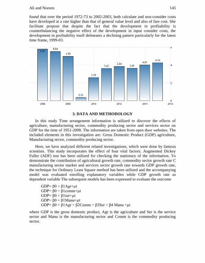
Ali and Noreen 145
found that over the period 1972-73 to 2002-2003, both calculate and non-consider costs
have developed at a rate higher than that of general value level and also of fare cost. She
facilitate propose that despite the fact that the development in profitability is
counterbalancing the negative effect of the development in input consider costs, the
development in profitability itself delineates a declining pattern particularly for the latest
time frame, 1999-03.
3. DATA AND METHODOLOGY
In this study Time arrangement information is utilized to discover the effects of
agriculture, manufacturing sector, commodity producing sector and services sector on
GDP for the time of 1951-2008. The information are taken from open door websites. The
included elements in this investigation are: Gross Domestic Product (GDP) agriculture,
Manufacturing sector, commodity producing sector.
Here, we have analyzed different related investigations, which were done by famous
scientists. This study incorporates the effect of four vital factors. Augmented Dickey
Fuller (ADF) test has been utilized for checking the stationary of the information. To
demonstrate the contribution of agricultural growth rate, commodity sector growth rate C
manufacturing sector market and services sector growth rate towards GDP growth rate,
the technique for Ordinary Least Square method has been utilized and the accompanying
model was evaluated enrolling explanatory variables while GDP growth rate as
dependent variable The subsequent models has been expressed to evaluate the outcome
GDP= β0 + β1Agr+µt
GDP= β0 + β1comm+µt
GDP= β0 + β1ser+µt
GDP= β0 + β1Manu+µt
GDP= β0 + β1Agr + β2Comm + β3Ser + β4 Manu +µt
where GDP is the gross domestic product, Agr is the agriculture and Ser is the service
sector and Manu is the manufacturing sector and Comm is the commodity producing
sector.

Effect of All Sectors on GDP Output Fluctuations in Pakistan Economy 146
3.1 Hypothesis
To direct our observational investigation we have figured an arrangement of working
hypothesis which take a solid adaptation of the engine to developed hypothesis for
purpose of departure. We take the log returns of all values before analyzing them.
a) Effect of Agriculture on GDP
b) Effect of Commodity on GDP
c) Effect of Manufacturing on GDP
d) Effect of all variables on GDP
Table 1
Regression Results of Relationship between AGR and Explanatory Variables
a) Effect of Agr on GDP
b) Effect of Comm on GDP
c) Effect of Manu on GDP

Ali and Noreen 147
d) Effects of all sectors on GDP
Variable Coefficient Std. Error t-Statistic Prob.
C 1.889579 0.385607 4.900275 0.0000 Agriculture 0.063503 0.092113 0.689400 0.4936 Manufacturing 0.100405 0.067633 1.484559 0.1436 Commodity Producing Sect 0.469883 0.124337 3.779124 0.0004
R-squared 0.750786 Mean dependent var 5.154561 Adjusted R-squared 0.736680 S.D. dependent var 2.477988 S.E. of regression 1.271573 Akaike info criterion 3.385978 Sum squared resid 85.69560 Schwarz criterion 3.529350 Log likelihood -92.50038 Hannan-Quinn criter. 3.441697 F-statistic 53.22294 Durbin-Watson stat 1.574803 Prob(F-statistic) 0.000000
Dependent Variable: GDP Method: Least Squares Date: 01/06/17 Time: 00:11 Sample: 1 57 Included observations: 57
Regression outcomes with explanatory variables are given in Table II. The outcomes
indicate that 1% expansion in the manufacturing growth rate acquires 10.04% expansion
in GDP growth rate. 1% expansion in the commodity sector growth rate acquires 46.96%
expansion in GDP growth rate. 1% expansion in the agriculture growth rate acquires
6.35% expansion in GDP growth rate. The coefficients are significantly at both 1% and
5% level of significance as demonstrated by low estimations of "P" in Table II. Results
indicates that due to agriculture the variation in DGP is 49% and due to commodity
sector is 73% and manufacturing sector is 26%.
The high estimation of R-square (0.75) which shows that 75% variation in GDP
explained by explanatory variables proposes that the fit is great and the included
independent variables are accountable elements for changes in GDP growth rate.
Durbin-Watson esteem (1.57) suggests positive serial autocorrelation. The Durbin
Watson measurement is utilized to tests for 1st order autocorrelation in the residuals in
regression analysis The Durbin-Watson value is lie between 1.5 and 2.5. here D.W value
is 1.57 which is closed to 1.5 implies that there is no autocorrelation in the residuals.
Values moving toward 1.5 demonstrate positive autocorrelation between the residuals.
GDP = 1.889579 + 0.063503Agr + 0.469883Comm + 0.100405Manu + µt

Effect of All Sectors on GDP Output Fluctuations in Pakistan Economy 148
(A) (B)
(C)
Graph A shows that there is a liner relationship between GDP and commodity
producing sector because trend exits means mean doesn’t same and the variance is not
constant and not all the values is move in same fluctuation and there is no seasonality is
exit and no outlier exits because some values are from the data
Graph B shows that there is a liner relationship between GDP and manufacturing
sector of economy because trend exits means mean doesn’t same and the variance is not
constant and not all the values is move in same fluctuation and there is no seasonality is
exit and no outlier exits because some values are from the data
Graph C shows that there is a liner relationship between GDP and agriculture sectors
because trend exits means mean doesn’t same and the variance is not constant and not all
the values is move in same fluctuation and there is no seasonality is exit and no outlier
exits because some values are from the data.

Ali and Noreen 149
Results of ADF Test
Variables t-Statistic Levels Conclusion
Gdp -6.90831 0.00 0(0)
Agr -9.747127 0.00 0(0)
Manu -4.348654 0.001 0(0)
Ser -5.995383 0.00 0(0)
Comm -7.943284 -7.94 0(0)
ADF (augmented dickey fuller test) is used to check the stationary of data for
acceptance or rejection of null hypothesis. Here results shows that all the variables are
stationary on levels and have a significant value on level. That shows null hypothesis is
not rejected because t*<critical test values means unit root does exit data in stationary on
level. After completing the observation that all variables are stationary on level.
3.2 Discussion
Volatility in Growth of Agriculture Sector:
The fluctuation in agriculture sector positively influenced the volatility of national
output growth. For overall economic development agriculture sectors considered key
determinants for economic progress. Earning of foreign exchange, generating income,
enhancing food production agriculture sector play a vital role in it. The economy cannot
function and survive without the without agriculture and industry because both are the
two hands of economy.
Volatility in Growth of Manufacturing Sector
The fluctuation in manufacturing sector is also positively influenced the volatility of
national output growth. For overall economic development manufacturing sectors also
considered key determinants for economic progress commodity producing sector
Volatility in Growth of commodity producing sector
The fluctuation in commodity producing sector is also positively influenced the
volatility of national output growth. For overall economic development commodity
producing sector also considered key determinants for economic progress commodity
producing sector.
4. CONCLUSION
The fundamental target of the study to check the fluctuations in national output by the
contribution of volatility. The volatility in sectors has been findings by this study. The
effect of agriculture, commodity producing sector and manufacturing sector on volatility
in national output is highly significant. The fluctuation in agriculture sector,
manufacturing sector and commodity producing sectors are positively influenced the
volatility of national output growth. For overall economic development all sectors
considered key determinants for economic progress. Earning of foreign exchange,
generating income, enhancing food production agriculture sector play a vital role in it.
The economy cannot function and survive without the without agriculture sector,
manufacturing sector and commodity producing sectors because all are the two hands of
economy.

Effect of All Sectors on GDP Output Fluctuations in Pakistan Economy 150
5. ACKNOWLEDGEMENT
I am utilizing this chance to express my appreciation to everybody who strengthened
me over the span of this M.Phil. projects. I am grateful for their trying direction,
pricelessly useful feedback and friendly advice amid the venture work. I am genuinely
appreciative to them for sharing their honest and enlightening perspectives on various
issues identified with the venture.
REFERENCES
1. So, H.M., Tse, R.Y.C. and Ganesan, S. (1997). Estimating the influence of transport
on house prices: evidence from Hong Kong. Journal of Property Valuation and
Investment, 15(1), 40-47.
2. Pasha, H.A., Ghaus, A. and Hyder, K. (2002). The slowing down of the growth of
total factor productivity in Pakistan. Social Policy and Development Centre Report
No. 44.
3. Shahida, W. (2002). The Rise and fall of Industrial Productivity in Pakistan. Oxford
University Press, Karachi.
4. Iffat, A. (2004). Is Pakistan’s manufacturing sector competitive? The Pakistan
Development Review, 43(4-2), 685-706.

151
Proc. ICCS-14, Multan, Pakistan
December 12-15, 2016, Vol. 30, pp. 151-158
IMPACT OF TERRORISM ON THE SUPPLY CHAIN OPERATIONS
AT KARACHI - PAKISTAN
Hashmat Ali1 and Faisal Afzal Siddiqui
2
1 Department of Management Science, Bahria University,
Karachi, Pakistan. Email: [email protected] 2 Business Research Consultants, Karachi, Pakistan
Email: [email protected]
ABSTRACT
In the aftermath of 9/11 terrorist attacks on the US World Trade Centers, a paradigm
shift has come to surface with regard to security threats to the inbound and outbound
logistics, the seller-purchaser relations, suppliers, clients and partners, in both the public
and private sectors’ commercial and trade activities. Today indiscriminate terrorist acts in
any form and kind can be expected anywhere.
This study is an effort to estimate the impact of terrorism on supply chain operations
in Karachi - Pakistan. The respondents are the supply chain managers from different
organizations across diverse industries from Karachi. The sample size is 100 respondents.
This study found that terrorism is damaging the supply chain operations and
organizations face crisis due halt in their supply chain operations in Karachi. The study
recommends the steps for institutional development regarding mitigating the impact of
terrorism on the supply chains operations.
KEYWORDS
Supply chain operations, crisis, terrorism, inbound, outbound, mitigation Karachi.
1. INTRODUCTION
In the aftermath of September 11th
terrorist attacks on the US World Trade Centers, a
paradigm shift has come to surface with regard to security threats to the inbound and
outbound logistics, the seller-purchaser relations, suppliers, clients and partners, in both
the public and private sectors’ commercial and trade activities. Soon after the attacks,
organizations working on “Just-in-Time” (JIT) lines, experienced huge losses as a result
of stoppage or inordinate delay in receipt of their inbound supplies (raw material)
required to transform same into finished goods required by their valued customers.
Today indiscriminate terrorist acts in any form and kind can be expected anywhere
e.g. Public Places, Motels/Hotels, Production/Manufacturing units, Under construction/
Private Buildings, Schools/Colleges, Health care centers, Militaries facilities/
installations, Pharmaceutical Companies, shipping/aircrafts, commercial/electronics
market and state owned offices/premises which can be sources of supplies/materials and
can definitely impact the supply of goods and services to industries. It has, therefore,

Impact of terrorism on the supply chain operations at Karachi - Pakistan 152
become a challenge for Supply Chain Managers to anticipate terrorism acts, plan
countermeasures towards it, plan, test and implement strategic preparedness steps.
The paper attempts to recognize the essential elements of supply chain operations at
Karachi which are impacted due to terrorism. This study differs in several aspects from
the prevailing surveys under taken on the subject. Few of the distinctive aspects are that it
uses actual data collected from the diverse business industries at Karachi. Previous
researches on the subject have observed the commercials arenas on a much lesser
frequency data. Therefore, this survey is unique in the sense that it is Karachi specific.
We have examined the effect of terrorism on each essential element which harms the
smooth supply chain operations.
2. LITERATURE REVIEW
Although studies are available discussing the causes of various uncertainties in supply
chains due one reasons or the other and impact of terrorism on financial markets,
economy and business etc., however no work related to our topic is available. The
empirical literature indicates that the impact of terrorism on supply chain operations is
multifaceted.
Gary and Michael (2008) declare the object of terrorist activities is to terrorize the
general public and build pressure on governments to achieve a political goal. Terrorism
has directly or indirectly affected the world businesses and the terror attacks have a big
impact on international supply chain. Due to the fear of terrorist activities the supply
chain has especially failed to deliver the goods effectively and efficiently.
Yi et al. (2011) identifies flexible supply chain in a stable environment using multiple
instances of the textile and apparel companies in China. The study shows the result of
four important strategies for supply chain to be flexible in an unstable environment,
innovation, operating efficiently and traditional response.
Soon after the terrorist attacks on 11th
September 2001, various companies including
Ford were compelled to stop their assembly lines intermittently, supply of raw materials
and spares etc. were stopped at the border of Canada and Mexico due security clearance.
Resultantly the companies lost large quantity of production units. Ford lost 12,000 units
of its production. The companies like Toyota which were working on JIT inventory
discipline halted production with a few hours subsequent to the attack. According to the
wall Street Journal (2001), due to disruption of steering sensors on account of shut down
of air travel from Germany, production in one of its plants in Princeton, Indian (IN),
came to a halt within 15 hours of the event of 9/11.
Tafur (2011) considers the grave impact of terrorism on the flow of international trade
from the United States and other countries. Supply chain activities in ports and in
oceans/seas is the single most important factor in the supply chain of the nation and these
have not been saved from terrorist attacks.
According to Ahmad et al. (2013) safety and security are the issues most important to
the tourist while traveling, and the first priority is that they consider to be protected from
the dangers.

Ali and Siddiqui 153
Dean et al. (2010) investigates how to minimize the risks faced by global sourcing
and selecting the best supplier in an environment of uncertainty through the use of
multiple criteria optimization technique, natural disasters, terrorist, social, political,
culture, labor and other variables. The author suggests that these tools contribute to a high
grade risk and businessmen are to make strategies to eliminate or reduce its impact on the
supply chain and business.
Claudia (2013) argues that can you imagine life without the places where we gather?
These are convenient places; places where we want to go, free to go. In airports,
stadiums, railway stations, cinemas, parks etc. you can control access. You have a part to
play to ensure freedom does not make you vulnerable. When people gather together
freely, it offers an opportunity for those who want to cause chaos.
Konova (2012) discusses many qualitative studies have been carried out against
terrorism and the events of September 11, 2001 have generated interest in the "war on
terror" discourse further. Focusing on different aspects of the phenomenon, scholars have
studied both the reasons and consequences.
Manuj and Mentzer (2008) investigates the risk mitigating approaches in the
international and domestic supply chain more important than before because they
consider global supply chain exposed to more threat than domestic one. The authors use
experimental research methods by interviewing senior executive through fourteen
detailed interviews with senior executives of manufacturing companies. The study
discloses 6 vital strategies for mitigating global sourcing risks.
Blos et al. (2009) analyze the risks faced by today’s supply chain and its mitigating
management throughout the operations of supply chain studying the electronics industry
and cars in Brazil. The study confirms that mitigating and controlling the risks and threats
to the supply chain operations ensure increase in company’s profitability and drastically
decreasing its losses.
Wei and Yang (2012) examine the role of risk management in the effectiveness of the
security in the supply chain operations from the shipping company for containers in
Taiwan. The results showed that all the variables (the management of relations with
suppliers over the long term, management and exchange of information, and the
reduction of accidents in the shipment and management skills) have a positive and
significant influence on the working of security matters whereas positive effect on
clearance can be ensured through engaging trusted, registered and pre-qualified supplier
through sustaining good business relations.
While finding out the impact of terrorism on the supply chains operations at Karachi,
the Dependent Variable (DV), we categorized the impact into eight distinct Independent
Variables (IVs). Keeping in view the impact of terrorism, whether directly or indirectly,
on the supply chain operations at Karachi, following model has been made in support of
the study.

Impact of terrorism on the supply chain operations at Karachi - Pakistan 154
3. THEORETICAL FRAMEWORK
INDEPENDENT VARIABLES DEPENDENT VARIABLE
4. OBJECTIVES
The objective of undertaking this study is to analyze whether terrorism has any
impact on the supply chain operations at Karachi - Pakistan. The topic of threat and risks
to the supply chain due terrorism has been studied by the researchers around the globe.
They have studied it from different perspectives i.e. risks faced by global sourcing,
supply chain internationally and domestic resource mobility. All the researchers have
deduced some conclusions from their studies. Most of the researchers have studied this
topic from a qualitative angle as they showed the impact terrorism brings in qualified
terms.
WEEK GLOBAL BUSINESS RELATIONS
INCREASED SAFETY STOCK LEVELS
SHORTAGE OF TRANSPORT
STOPPAGE OF PRODUCTION
DISRUPTION OF RAW MATERIALS
PRICE HIKE
STOPPAGE OF FDI
HIGH COST OF INPUTS
CAPITAL TRANSFER
INFRASTRUCTURE LOSS
COST OF SECURITY EQUIPMENT
RIVAL BENEFIT
SUPPLY
CHAIN
OPERATIONS

Ali and Siddiqui 155
5. RESEARCH DESIGN
Sampling Procedure
Keeping in view the data, a number of organizations were identified, short listed and
randomized in to a representative unit of about 10 Industries. Keeping in view the
requirement for the data a comprehensive study device was designed, with due reference
to prevailing terrorism threat to business sector in Karachi - Pakistan. This research is
specific to the existing threat of terrorism being experienced by business sector and the
events already taken place in Karachi - Pakistan.
Data Source
One hundred organizations were shortlisted from ten different sectors, consisting of
local and multi-national organizations including SMEs. The shortlisted industries
comprised of consumer products/services, leather and shoes, energy and fuel, fertilizer
and chemical, building and cement, pharmaceuticals, textile, financial companies,
IT/Telecom etc.
After identifying the potential respondents, questionnaires were sent directly to them.
After a gap of 3-4 days, a trained data collector personally visited the respondents to
clarify the queries, if any, and collect the filled survey forms. The factors of flexibility
and adaptability were catered for in the methodology.
Statistical Tool Used Multiple regression analysis was used through the well-known software package
SPSS version 20 to assess the impact of the IVs on the DV.
6. RESULTS
We estimated the impact of terrorists’ activities on the supply chain operations
through eight independent variables. A total of four out of the eight categories have
negative impact on the supply chain operations. The below tables show the results;
Table 1: Model Summary
Model R R Square Adjusted R Square Std. Error of the Estimate
1 .482a .232 .164 26.52100
a. Predictors: (Constant), Rival country takes benefit, Increasing level of Safety Stock,
Cost on purchase of Sec Eqpt, Stoppage of Production, Infrastructure Loss, Distrust
in Global Bus Relations, Disruption of raw material, Increase in Cost of Inputs.
b. Dependent Variable: Supply Chain Operations
Model Summary Table
R² =.232 taken as a set, the predictors (IVs 1-8) account for 23% of variance in DV.
It does not show how much individual IV accounts for.R² is significant if greater than
zero (0).

Impact of terrorism on the supply chain operations at Karachi - Pakistan 156
Table 2: ANOVA
Model Sum of Squares Df Mean Square F Sig.
1
Regression 19318.906 8 2414.863 3.433 .002b
Residual 64006.094 91 703.364
Total 83325.000 99
a. Dependent Variable: Supply Chain Operations
b. Predictors: (Constant), Rival country takes benefit, Increasing level of Safety Stock,
Cost on purchase of Sec Eqpt, Stoppage of Production, Infrastructure Loss, Distrust in
Global Bus Relations, Disruption of raw material, Increase in Cost of Inputs
ANOVA Table (test using alpha = .05)
The overall regression model is significant
F(8,91) = 3.433, p=.002, R²=.232
Table 3: Coefficients
Model
Unstandardized
Coefficients
Standardized
Coefficients t Sig.
Collinearity
Statistics
B Std.
Error Beta Tolerance VIF
1 (Constant) 168.930 42.117 4.011 .000
Disruption of raw
material -29.930 12.188 -.387 -2.456 .016 .339 2.948
Stoppage of
Production 12.876 5.631 .243 2.287 .025 .745 1.342
Increasing level of
Safety Stock -31.739 10.837 -.381 -2.929 .004 .499 2.004
Increase in Cost of
Inputs 53.881 19.333 .589 2.787 .006 .189 5.293
Infrastructure Loss 3.302 6.816 .058 .484 .629 .595 1.680
Cost on purchase of
Sec Eqpt .609 3.388 .018 .180 .858 .821 1.217
Distrust in Global
Bus Relations -30.038 17.790 -.311 -1.688 .095 .249 4.009
Rival country takes
benefit -8.128 7.108 -.117 -1.144 .256 .811 1.233
a. Dependent Variable: Supply Chain Operations
Coefficient Table
(Test each predictor at alpha=.05)
1. Disruption of raw material sig. (p=.016)
2. Stoppage of production sig. (p=.025)
3. Increased safety stock levels sig. (p=.004)
4. High cost of inputs sig. (p=.006)
5. Infrastructure loss not sig. (p=.629)
6. Cost of security equipment not sig. (p=.858)
7. Weak global business relations not sig. (p=.095)
8. Rival benefit not sig. (p=.256)

Ali and Siddiqui 157
7. OVERALL ANALYSIS
A multiple liner regression was calculated to predict “Supply chain Operations” (DV)
based on Disruption of Raw Materials (IV1), Stoppage of Production (IV2), Increased
Safety Stock Levels (IV3), High Cost of Inputs (IV4), Infrastructure Loss (IV5), Cost of
Security Equipment (IV6), Weak Global Business Relations (IV7) and rival Benefit
(IV8). A significant regression equation was found (F (8,91) = 3.433, p = .002), with an
R² of .232.
Participants’ predicted (DV) is equal to 168.930 – 8.128 (IV8) – 30.038 (IV7)+ .609
(IV6) +3.302 (IV5) + 53.881 (IV4) – 31.739 (IV3) + 12.876 (IV2), - 29.930 (IV1),
whereas all (IVs) are coded or measured as 1 = Strongly Disagreed, 2 = Disagreed,
3 = Neutral, 4 = Agreed and 5 = Strongly Agreed.
Participant’s weight increased 168.930 [DV unit of measure] for each IV.IV1, IV2,
IV3, and IV4, were found significant predictors of DV.
8. COMMENTS AND CONCLUSIONS
Aim of the investigation was to assess the impact of terrorism on the supply chain
operations at Karachi - Pakistan. The findings of the regression model enable us to
conclude; that the supply chain operations at Karachi - Pakistan have been badly affected
by the prevailing uncertainty due terrorism. The volatile security situation has badly and
significantly damaged the effectiveness of the fundamentals (raw material, transportation,
production, global business relations, costs of inputs, price hike etc) of supply chain
operations. Result of the study is matching the theoretical framework and meeting the
expectations. The upward pace of terrorism is, undoubtedly, badly affecting the business
and affecting the country’s economy. Businesses will continue to be targets of the
terrorist activities mainly to weaken the financial position of the country.
9. ACKNOWLEDGEMENT
All thanks to ALLAH ALMIGHTY, the benevolent and compassionate, who blessed
me with the power & capabilities and remained contented on all intricacies found during
the successful completion of my task. I extend my special thanks to my Supervisor for his
encouraging response and guidance to make my Research Project a real learning
experience. I also acknowledge my parents and kids for their prayers, my Wife for her
throughout support in fulfilling social life obligations and teachers for their guidance
because I think all these are indispensable for success in every stage of life.
REFERENCES
1. AlBattat, A.R. and Mat Som, A.P. (2013). Emergency preparedness for disasters and
crises in the hotel industry. SAGE Open, 3(3), 2158244013505604.
2. Claudia Aradau (2013). CBRNE hardening of Airports, Shopping Malls and Luxury
hotels & resorts. CBRNE E-Journal News Letterrorism Issue, 50, 2013.
3. Konova, E. (2013). Rhetoric Techniques of Labeling of Environmentalists as
"Terrorists": the Case of the Earth Liberation Front in the United States of America,
1996-2006.

Impact of terrorism on the supply chain operations at Karachi - Pakistan 158
4. Yang, C.C. and Wei, H.H. (2013). The effect of supply chain security management on
security performance in container shipping operations. Supply Chain Management:
An International Journal, 18(1), 74-85.
5. Tafur Altiok (2011). Port security/safety, risk analysis, and modeling Ann Oper Res
(2011). Springer Science & Business Media, LLC 2011.
6. Yi, C.Y., Ngai, E.W.T. and Moon, K.L. (2011). Supply chain flexibility in an
uncertain environment: exploratory findings from five case studies. Supply Chain
Management: An International Journal, 16(4), 271-283.
7. Deane, J.K., Craighead, C.W. and Ragsdale, C.T. (2009). Mitigating environmental
and density risk in global sourcing. International Journal of Physical Distribution &
Logistics Management, 39(10), 861-883.
8. Natarajarathinam, M., Capar, I. and Narayanan, A. (2009). Managing supply chains in
times of crisis: a review of literature and insights. International Journal of Physical
Distribution & Logistics Management, 39(7), 535-573.
9. Blos, M.F., Quaddus, M., Wee, H.M. and Watanabe, K. (2009). Supply chain risk
management (SCRM): a case study on the automotive and electronic industries in
Brazil. Supply Chain Management: An International Journal, 14(4), 247-252.
10. Knight, G.A., Czinkota, M.R., and Liesch, P. (2008). Terrorism and International
Business, Working Paper, 1-23.
11. Manuj, I. and Mentzer, J.T. (2008). Global supply chain risk management strategies.
International Journal of Physical Distribution & Logistics Management, 38(3),
192-223.
12. Khalid, S. (2008). Trend forecasting for stability in supply chains. Journal of Business
Research, 61, 1113-1124.
13. Kros, J.F., Falasca, M. and Nadler, S.S. (2006). Impact of just-in-time inventory
systems on OEM suppliers. Industrial Management & Data Systems, 106(2),
224-241.

159
Proc. ICCS-14, Multan, Pakistan
December 12-15, 2016, Vol. 30, pp. 159-167
A CASE STUDY OF FACTORS AFFECTING MONEY DEMAND IN
PAKISTAN: AN ECONOMETRIC STUDY USING TIME SERIES DATA
Muhammad Yousaf1 and Syed Anwer Husnanin
2
1 Punjab Education Foundation, Lahore, Pakistan
Email: [email protected] 2
National College of Business Administration and Economics
Lahore, Pakistan. Email: [email protected]
ABSTRACT
Money demand function plays a key role in monetary policy formulation. In this
paper, we have examined the determinants of money demand function in Pakistan using
time series data from 1972 to 2010. By using the OLS estimation technique, important
findings of this paper i.e. population growth, per capita income and financial innovation
are positively affecting demand for money. While inflation rate and exchange rate are
negatively related to money demand in Pakistan. Breusch – Godfrey serial correlations
LM test shows no problem of autocorrelation in both the models. Ramsey RESET test
examines that model is correctly specified. On the basis of results demand of money may
be controlled through controlling inflation, population growth rate, per capita income,
exchange rate and financial innovation.
KEYWORDS
Population Growth, Financial Innovation, Exchange rate, Ordinary Least Square
Method.
1. INTRODUCTION
Everlasting rises of developing countries are worldwide economic crises that become
a new challenge for them. World Bank is becoming a source of financial help but many
millions of the people are focusing on this financial aid. This economic chaos is
spreading speedily and the filter of it is prevailing in the all of the World, together with
Asian countries. Losing investors’ wealth is an obstacle among Asian countries. Panic
selling of goods becomes alarming in the stock markets of the world and become a cause
of falling worldwide capital markets. A situation in which the money supply will be more
than the demand for money represents financial crises. One main factor that affects the
amount of demands for money is the uncertain circumstances of the financial market that
economic representatives want to keep.
Demand for Money is currently an important policy implication debate in the world
especially in Asia. A well specified demand for money has a greater importance for the
regulation of stable monetary as well as much more important for Pakistan economy. The
demand for money arises from two important functions of money. The first is that money
acts as medium of exchange and the second is that it is a store of value. Thus individuals
and businesses wish to hold money partly in cash and partly in the form of assets. There

A Case Study of Factors affecting Money Demand in Pakistan:…. 160
are three approaches to demand for money; the Classical, the Keynesian, and the post –
Keynesian. The classical economists did not explicitly formulate demand for money
theory but their views are inherent in the quantity theory of money.
The purpose of the study is to examine the determinants of money demand function
based on broad and narrow money on the economy of Pakistan. After the theoretical
framework in first section, the rest of the paper is organized as follows; Section second
discusses literature review, Section third presents the data and methodological issues,
section forth is consisting upon results and discussion and finally Section five is
regarding conclusions and policy recommendations.
2. LITERATURE REVIEW
A vast literature is available on the topic money demand function nationally as well as
internationally. This section summarizes few of them as follows. Fisher (1911)
emphasized on the transactions demand for money in terms of velocity of circulation of
money. This is because money acts as a medium of exchange and facilitates the exchange
of goods and services. Transactions demand for money is determined by the level of full
employment income. This is because the classical believed in Say’s Law whereby supply
created its own demand, assuming the full employment level of income. Thus the demand
for money in Fisher’s approach is a constant proportion of the level of transactions which
in turn bears a constant relationship to the level of national income. Further, the demand
for money is linked to the volume of trade going on in an economy at any time. People
hold money to buy goods and services, to earn interest and to provide against unforeseen
events.
Keynes (1936) abandoned the classical view that velocity was a constant and
developed a theory of money demand that emphasized the importance of interest rates.
His theory of the demand for money which he called the liquidity preference theory asked
the question: Why do individuals hold money? He postulated that there are three motives
behind the demand for money: the transactions motive, the precautionary motive and the
speculative motive. Transactions and Precautionary demand for money is a positive
function of income but speculative demand for money is inversely influenced by interest
rate.
Baumol (1952) analyzed the interest elasticity of the transactions demand for money
on the basis of his inventory theoretical approach. He showed that the relation between
transactions demand and income is neither linear nor proportional. Rather, changes in
income lead to less than proportionate changes in the transactions demand for money.
Tobin (1956) formulated the risk aversion theory of liquidity preference based on
portfolio selection. This theory removed two major defects of the Keynesian theory of
liquidity preference. One, Keynes’s liquidity preference function depended on the
inelasticity of expectations of future interest rates and two individuals hold either money
or bonds. His theory did not depend on the elasticity of expectations of future interest
rates but proceeds on the assumption that the expected value of capital gain or loss from
holding interest – bearing assets is always zero. Moreover, it explains that an individual’s
portfolio was holding money and bonds rather than only one at a time.

Yousaf and Husnanin 161
Friedman (1956) recognized that people want to hold a certain amount of real money
balances. His real money demand function was a function of wealth (permanent Income),
expected return on money, expected return on bonds, expected return on equity and
expected inflation rate.
Rehman and Afzal (2003) empirically the impact of black market exchange rate on
demand for money in Pakistan where official and black market exchange rate operates
side by side due to exchange control. They gathered time series data during 1972-2000
following autoregressive and Distributed lag model for estimation. The authors
concluded that real income peroxide by industrial production and black market exchange
rate were increasingly affected by desired holding of real money balances and inflation
was negatively influenced by desired holding of real money balances. They suggested
that M2 monetary aggregate was the right aggregate to be considered for affective policy
formulation.
Qayyum (2005) explored to estimate the dynamic demand for money function in
Pakistan that could be used for policy analysis. They gathered time series data during
1960-1999 following Johansen co-integration technique. They concluded rate of inflation
was negatively inducing in long run money demand function. Long run income was
positively related to money demand function.
Khan and Sajjid (2005) had investigated both the long run and short run relationship
between real money balances, real income, inflation rate, foreign investment rate and real
effective exchange rate, They utilized time series data during 1982-2002 following auto
regressive distributed lag approach for estimation. The study concluded that real GDP
was giving positive effect on nominal money balances. Interest rate and Inflation were
negatively related to nominal money balances. They suggested rebalancing effect
resulting from variations in the real exchange rate that played a key role in Pakistan’s
money demand behavior.
Valadkhani (2008) examined the long and short run determinants of the demand for
money in six countries .They collected panel data during 1975-2002. They concluded that
real income had positively related to demand for real balances and interest rate spread.
Inflation rate, real effective exchange rate and real interest rate were negatively related to
demand for real balances. They suggested real M2 was a predictable monetary aggregate.
They estimated long run income elasticity for all six countries exceeded unity.
Arshad (2008) made to reformulate and estimate the MABP for Pakistan. They made
use of time series data during 1962 to 2005 following the Fully Modified Ordinary Least
Square method and Johansen cointegration technique for estimation. The Author
concluded that real income and real exchange rate were positively related to the money
demand function in real term, and interest rate was negatively related to the money
demand function in real term. They suggested that inverse relationship between foreign
reserve and domestic credit recommend that the authorities may restrict the borrowing
from the State Bank of Pakistan.
Hye et al. (2009) had explored to estimate the association between exchange rates,
stock prices, and demand for money function in Pakistan. They made use of time series
data during 1971 to 2006 following Johansen co-integration technique for estimation. The
A Case Study of Factors affecting Money Demand in Pakistan:…. 162
authors concluded that economic activity, inflation and stock prices were positively
influencing money demand and exchange rate and interest rate had negative affect on
money demand. The analysis recommended an increase in stock price dictated an easier
monetary policy to prevent a given nominal income or inflation target being undershot.
Omer (2010) evaluated to contribute to the ongoing debate; should central bank of
Pakistan adopted the inflation targeting or continued with the monetary targeting as a
monetary policy strategy. They collected time series data and employed Auto regressive
and Distributed lag model for estimation. The analysis concluded that real permanent
income per capita, real interest and expected inflation were directly affecting income
velocity of money and transitory income was negatively affecting to income velocity of
money. They suggested monetary authorities of Pakistan Mo and M2 as nominal anchors
for operational and intermediate targets respectively while it had never used M1 officially
for policy purpose.
Rutayisire (2010) explored to estimate the function of demand for money in short run
and in long run for Rwanda economy. He utilized time series data during 1980-2005
following Johansen co-integration technique for estimation. They concluded that Log of
real income was inducing M2. Central bank financing rate, the London interbank offered
rate and the anticipated fluctuation of RWF exchange rate representing money
depreciation were negatively influencing the log of M2. They suggested no significant
role of interest rates in the demand for money in Rwanda. This suggested that the
refinancing rate and BNR’S key interest rate had no effect on the composition of people’s
portfolio.
Sarwar et al. (2010) evaluated the money demand function that played a key role in
monitory policy formulation. They utilized time series data following Auto regressive
and Distributed lag model for estimation. The study concluded that log of real GDP and
log of financial innovation were directly related to reserve money and price was
negatively influenced by reserve money.
Suliman and Dafaalla (2011) made attempt to test the existence of stable money
demand function in Soudan. The analysis collected time series data during 1960-2010
following co-integration technique for estimation. The study concluded that real income
was affecting effecting on demand for real money balances and Inflation and exchange
rate were negatively affecting to demand for real money balances. They recommended
that it was possible to use the narrow money aggregate as target of monetary policy in
Sudan
3. DATA AND METHODOLOGY
To analyze the factors determining money demand, the empirical equations are being
modeled as below;
0 1 2 3 4 5
0 1 2 3 4 5
2
0
M POPG PCI INF FINO ER
M POPG PCI INF FINO ER
In the above mentioned models, we have used the following variables.

Yousaf and Husnanin 163
Dependent Variable
M2 = Broad Money
M0 = Narrow Money
Explanatory Variables
POPG = Population Growth rate
PCI = Per Capita Income
INF = Inflation rate
FINO = Financial Innovation
ER = Exchange rate
and = Error Terms
' , 's s = Coefficients of variables
The current paper has utilized time series annual data for the time period from 1972 to
2010. The main sources of data are Handbook of statistics on Pakistan Economy 2010,
Economic Survey of Pakistan (2010 – 11) and Statistical Year book 2010. We have
employed Ordinary Least Square method to examine coefficients of regression equation
and then applied some Diagnostic tests to find out Econometric problems. On the basis of
Past studies and Hypothesis, the expected signs of explanatory variables are shown in the
following Table 1.
Table 1
Expected Signs
4. RESULTS AND DISCUSSION
In Table 2, values for Mean, Minimum, Maximum and Standard Deviation are given
corresponding to the variables. In the above table M2 and M0 are dependent variable and
POPG, PCI, INF, FINO and ER are independent variables. The sample size comprises of
38 observations from the period of 1972 to 2010. The minimum and maximum values of
M2 are 5137205 and 22059 respectively, whereas the mean value is 1040628 and
standard deviation is 1372136. POPG having minimum value is equal to 2.07, maximum
value is 3.24, mean value is 2.66 and standard deviation is 0.32. PCI has minimum value
1012.60, maximum value 75024.85, mean value 16927.07 and standard deviation
18711.36. Minimum and maximum values are respectively 2.46 and 23.87; similarly
mean and standard deviation are 9.94 and 5.12). Mean, Standard Deviation, minimum
and maximum values are respectively 0.40, 0.04, 0.29 and 0.46. Minimum and maximum
Variables Expected Sign
Population Growth Positive
Per Capita Income Positive
Inflation Negative
Financial Innovation Positive
Exchange Rate Negative

A Case Study of Factors affecting Money Demand in Pakistan:…. 164
values are 8.50 and 83.80 respectively. Whereas mean value is 31.29 and standard
deviation is 22.48. The minimum and maximum values of M0 are 8138 and 8138
respectively. Mean value is 335011.30 and standard deviation is 411813.60.
Table 2
Descriptive Statistics
M2 M0 POPG PCI INF FINO ER
Mean 1040628.0 335011.3 2.66 16927.07 9.94 0.40 31.29
Median 370947.5 155023.0 2.57 8571.28 9.39 0.40 22.75
Maximum 5137205.0 1507581.0 3.24 75024.85 23.87 0.46 83.80
Minimum 22059.0 8138.0 2.07 1012.60 2.46 0.29 8.50
Std. Dev. 1372136.0 411813.6 0.32 18711.36 5.12 0.04 22.48
Table 3 and 4 reports estimated results of regression model, in which columns 1, 2, 3,
4 and 5 respectively denote Variables, Coefficients, Standard Errors, T – Statistics, and
Probability values. Diagnostic tests are also mentioned at the end of table with their Null
Hypothesis, F – Statistics and probability values.
With regards to population growth, that is positively related to demand for broad and
narrow money with statistically significant coefficient. The rationale behind this
relationship is that when population is increased, there will be more people to consume
and it would lead to higher demand for broad and narrow money. Due to increase of one
percent population growth, demand for money will increase by rupees 395050 or 88952
on the average. Per capita income, it suggests positive relationship with broad and narrow
money having significant coefficient. Demand for broad and narrow money will increase
by rupees 93 or 24 if per capita income is increased by 1 rupee on the average. Reason
may be that more per person income lead to higher demand for broad and narrow money.
This result is matched with the study of Muhammad Omer (2010).
In this study, inflation rate is found to have negative relationship with demand for
broad and narrow money. It is statistically insignificant in both the models. Keeping
money income fixed when inflation rate increased, goods and services will be more
expansive, and it would be difficult for people to sustain their life style so ultimately
demand for broad and narrow money will decline. This relationship is consistent with the
studies of Khan and Sajjid (2005), Qayyum (2005), Rehman and Afzal (2003), Suliman
and Dafaalla (2011), Valadkhani (2008).
Financial innovation has positive sign in both the models and it is statistically
significant because its probability is less than 0.10. If financial innovation rate is
increased by one point then demand for money will increase by rupees 2188510 or
587854 on the average. While easy financial developments and sophistications in modes
of payments and lesser user cost in term of time and money for drawing the money
positively affect the demand for money. Our result is matched with the study of Sarwar et
al. (2010).

Yousaf and Husnanin 165
Table 3
Regression Estimates of Demand for Broad Money
Variable Coefficient Std. Error t-Statistic Prob.
C -1966300 482806.40 -4.07 0.00
POPG 395050.60 113058.50 3.49 0.00
PCI 93.07 3.04 30.53 0.00
INF -2051.63 3677.48 -0.55 0.58
FINO 2188510 561501.80 3.89 0.00
ER -15312.09 2722.13 -5.62 0.00
R-squared 0.79 F-statistic 1638.31
Adjusted R-squared 0.78 Durbin-Watson stat 1.94
Diagnostic Tests
Breusch-Godfrey Serial Correlation LM Test
F-statistic 1.16 Probability 0.28
Obs*R-squared 1.38 Probability 0.24
Null hypothesis: there is no problem of autocorrelation.
Ramsey RESET Test:
F-statistic 2.28 Probability 0.14
Log likelihood ratio 2.69 Probability 0.10
Null hypothesis: regression model is correctly specified.
Exchange rate is negatively related to demand for broad and narrow money. It is
statistically significant because its probability is less than 0.10. If exchange rate will
increase by one point then demand for broad and narrow money will decrease by rupees
15312 or 2273 on the average. Reason may be that due to increase in exchange rate,
foreign goods and services will be expansive for domestic customers, imports will
decline and ultimately it will affect demand for money in negative direction. Our results
are similar to comparable with the studies of Hye et al. (2009), Suliman and Dafaalla
(2011), and Valadkhani (2008).
Co-efficient of determination (R2
= 0.79, 78) shows that the 79 and 78 percent
variations in the dependent variable is explained variations in explanatory variables.
F – Statistics 1638.317 and the probability 0.00, explain that the overall regression model
is statistically significant. Durbin Watson statistics is 1.94 or 2.15, which is around 2
therefore there is no autocorrelation in the regression models. Bruesch – Godfrey Serial
Correlation test (Probability > 0.10) may not reject the null hypothesis and confirms the
absence of autocorrelation problem from the regression model. Ramsey RESET Test
(Probability > 0.10) also explains that regression models are correctly specified.

A Case Study of Factors affecting Money Demand in Pakistan:…. 166
Table 4
Regression estimates of Demand for Narrow Money
Variable Coefficient Std. Error t-Statistic Prob.
C -485508.70 190951.50 -2.54 0.01
POPG 88952.70 44715.02 1.98 0.05
PCI 24.99 1.20 20.73 0.00
INF -442.94 1454.45 -0.30 0.76
FINO 587854.70 222075.80 2.64 0.01
ER -2273.22 1076.61 -2.11 0.04
R-squared 0.78 F-statistic 940.70
Adjusted R-squared 0.77 Durbin-Watson stat 2.15
Diagnostic Tests
Breusch-Godfrey Serial Correlation LM Test
F-statistic 2.09 Probability 0.14
Obs*R-squared 4.66 Probability 0.09
Null hypothesis: there is no problem of autocorrelation.
Ramsey RESET Test
F-statistic 0.82 Probability 0.37
Log likelihood ratio 0.99 Probability 0.31
Null hypothesis: regression model is correctly specified.
5. CONCLUSIONS AND POLICY RECOMMENDATIONS
The study examines factors affecting money demand function on the economy of
Pakistan. Population growth, per capita income and financial innovation are found to
have positive influence on demand for money in Pakistan. Due to increase in population
growth and per capita income, people will consume more on goods and services. To
consume more, they need more money and ultimately demand for narrow and broad
money will increase. Financial innovation is positively related to money demand, as there
is financial innovation people want to purchase financial instruments (bonds, equity),
therefore people will demand money and money demand will increase. On the other side,
two most important variables; exchange rate and inflation are concluded to affect demand
for broad and narrow money indirectly in Pakistan. Reason may be that keeping income
constant, due to increase in price level, people can purchase less goods and services and
will demand less money. While an increase in exchange rate makes imports more costly,
people will consume less on imported items and will demand less as previous.

Yousaf and Husnanin 167
On the basis of results, the study suggests some policy implications that responsible
authorities should control population growth rate and per capita income because more
demand for goods and services will lead to higher price level which will affect the poor
nation of economy. Financial innovation is necessary element for the nation, as it leads to
higher internal savings, investment and exports as well. Inflation is harmful for
stabilization of the economy it should be controlled.
REFERENCES
1. Arshad, M.K. (2008). Long run and short run dynamics of foreign reserves and
domestic credit in Pakistan. International Journal of Applied Econometrics and
Quantitative Studies, 5(1), 61-84.
2. Baumol, W.J. (1952). Transactions demand for cash: An inventory theoretic
approach. Quarterly journal of Economics, 66, 545-556.
3. Fisher, I. (1911). The Purchasing Power of Money.
4. Friedman, M. (1956). The Quantity theory of Money: A Restatement. In Studies in
the Quantity theory of Money. University of Chicago Press, 9-21.
5. Hye, Q.M.A., Wasti, S.K.A., Khatoon, N. and Imran, K. (2009). Relationship
between stock prices, exchange rate and demand for money in Pakistan. Middle
Eastern Finance and Economics, 3, 89-96.
6. Jhingan, M.L. (2004). Monetary Economics, 6th
Edition.
7. Keynes, J.M. (1936). The General theory of Employment, Interest, and Money.
8. Khan, M.A., and Sajjid, M.Z. (2005). The exchange rate and monetary dynamics in
Pakistan: An Autoregressive Distributed Lag Model (ARDL) Approach. The Lahore
Journal of Economics, 10(2), 87-99.
9. Omer, M. (2010). Velocity of money functions in Pakistan and lessons for monetary
policy. SBP Research Bulletin, 6(2), 37-55.
10. Qayyum, A. (2005). Modeling the demand for money in Pakistan. The Pakistan
Development Review, 44(3), 233-252.
11. Ratayisire, M.J. (2010). Economic Liberalization, Monetary policy and money
demand in Rwanda 1980-2005. AERC Research Paper, 193, 1-30.
12. Rehman, H., and Afzal, M. (2003). The black market exchange rate and stability of
Demand for money in Pakistan: A Cointegration Analysis. Pakistan Economic and
Social Review, 41(1&2), 13-28.
13. Sarwar, H., Hussain, Z. and Sarwar, M. (2010). Money demand functions for
Pakistan. Pakistan Economic and Social Review, 48(1), 1-20.
14. Suliman, S. Z. and Dafaalla, H. A. (2011). An econometric analysis of money demand
function in Sudan 1960 - 2010. Journal of Economics and International Finance,
3(16), 793-800.
15. Tobin, J. (1956). The Interest Elasticity of the Transactions demand for Cash. Review
of Economics and Statistics, 38, 241-247.
16. Valadkhani, A. (2008). Long and short run determinants of demand for money in the
Asian Pacific countries: An Empirical Panel Investigation. Annals of economics and
Finance, 9(1), 47-60.

A Case Study of Factors affecting Money Demand in Pakistan:…. 168

169
Proc. ICCS-14, Multan, Pakistan
December 12-15, 2016, Vol. 30, pp. 169-178
ORGANIZATIONAL CHANGE AND UP-GRADATION
OF HIGHER EDUCATION INSTITUTIONS IN PAKISTAN
THROUGH INSTITUTIONAL PERSPECTIVE:
A CASE STUDY OF LAHORE COLLEGE FOR WOMEN UNIVERSITY
Nargis Akhtar1, Siama Zubair
2 and Muhammad Azam
2
1 Lecturer, Comsats Institute of Information Technology,
Vehari, Pakistan. Email: [email protected] 2 University of the Punjab, Lahore, Pakistan.
Email: [email protected]
ABSTRACT
The up-gradation of higher education institution in Pakistan is the continuation of the
change agenda of the government started in 1990‟s under the new public management
(NPM) reforms. Higher education institutions in general and policy making institutions
including Higher Education Commission of Pakistan in particular are focusing more on
restructuring the higher education institutions through various methods such as up-
gradation.
The present study evaluated up-gradation of Lahore College for women to a
University. Case study method was utilized for this research project. Twelve in-depth
interviews were conducted including Registrar, Deputy Registrar, Head of Departments,
Dean of faculty and Faculty members to collect the primary data. Using interpretive
perspective up-gradation process and changes introduced in University were discovered.
Theoretical rationalization of phenomenon is also elaborated in the light of institutional
theory and social political and agency pressures.
KEYWORDS
Up-gradation, New Public Management.
INTRODUCTION
Educational infrastructures of Western countries have encountered a big wave of
reforms, resulting in great improvements in the administration of higher educational
institutions. The systematic implementation of these reforms has affected the whole
world. Since education is a global phenomenon, the developing countries have begun to
feel the pressures in maintaining international standards of education and restructuring
their institutions according to higher education standards set by international institutions
(NEP, 2009; Azam, 2007).
In the pursuit of this reform agenda Higher Education Commission of Pakistan has
given guidelines to education institutions to adopt a standard set of practices to align with
international standards of education (Jahangir, 2008). Many higher education institutions

Organizational Change and Up-Gradation of higher education institutions… 170
are restructuring themselves in the light of Higher Education Commission guidance by
reforming and up-grading (Raouf, 2006).
The present study is conducted to study the changes introduces in LCWU after up-
gradation of a college to university. The major aim of the study is to observe
What changes are introduced in the administration of LCWU after up-gradation?
How up-gradation is carried out in LCWU?
LITERATURE REVIEW
In 1970‟s and 1980‟s transitional and developing countries of the world has observed
a wave of public sector management reforms. The major focus of these reforms was on
the role and institutionalization process of the countries and in introducing market
principles of profit maximization and greater efficiency in public sectors. These reforms
were started in developed nations and implemented on developing countries through
aided schemes of International Monetary fund and World Bank (Hughes, 1998).
The reasons behind these reforms were manifold including financial crisis and
enlarged size of government that raised serious questions on the role of state especially
when economy was derailing. In West, failure of Keynesian welfare state was basic
reason to introduce some new and innovative ways of governing. The fiscal crisis of
1970s and 1980s played important role in redefining responsibility of state and
introducing market principles of profitability and competition in government sector
(Marini, 1971). These techniques are being introduced in developing countries to
strengthen their unstable governments and to support them in establishing a sustainable
legal environment (OECD, 1993). NPM (new public management) is the label given to
these practices and techniques (Hood, 1991).
The vital element of NPM is the attempt to initiate or suggest the efficient ways of
work by introducing incentives and linking performance with promotion in public sector.
The primary supposition is that public sector can be more efficient by introducing private
sector principles of competition (Metcalfe and Richards, 1991).
BASIC CONCEPT OF NPM
The term is defined as:
“An innovative set of practices to deal with the public issues in a participative
way to increase efficiency in minimum possible time (OECD, 1993).”
NPM is collection of up to date ideas and practices that hunt for utilizing efficient
ways of service delivery. The basic idea is reforming structures in government sector by
introducing market base mechanisms and healthy competition (Denhardt & Denhardt
2003).These changing efforts were started in 1980s from that time this concept of change
and reforming governments is being practiced around the world with great success. NPM
focused on innovation, accountability, openness, organizational change, clarity, time
management, smart learning, project management, performance linkages, incentives and
flat structures (Gruening, 2001; Larbi, 1999; Polidano, 1999; Batley 1999; Pollitt &
Sorin, 2011).

Nargis, Siama and Azam 171
ORGANIZATIONAL CHANGE
NPM focuses on reforming organizations through organizational change.
Organizational change has always been a focus of the governments in the developing
world. As developing countries are facing issues of unstable political environment, weak
institutional structures and derailing economies. The administrative reforms introduced
under NPM agenda are apprehensive and encouraging for organizational change. These
reforms are more focused on structural and functional changes in developing countries in
order to change their organizational setup according to changing world. Education is the
most important tool for bringing change in developing countries. So; changes are
introduced through Higher Education in developing countries. Demand for education
grows as society undergoes development. Education teaches people and gives them
wisdom. During reform process education sector is the most important sector to be
considered and plays a vital role in development. So, while introducing reforms public
educational institutions cannot be neglected and these institutions should be introduced a
systematic reforms in order to make development process successful (Gabriele, 2000).
Western countries have introduced drastic changes in structure and pattern of higher
education during last twenty years. They introduced business sector practices to the
educational institutions to enhance their efficiency. They also encouraged developing
countries to embrace these trends education by offering funded higher education to their
students and by developing associations with their institutions. They also demanded
higher education institutions to change their structures according to international
standards to compete the developed countries in the field of education (Altbach &
Ogawa, 2001; Teichler, 2003).
DEFINING CHANGE MANAGEMENT
Change management is defined in a numerous ways in literature change is termed as
altering organizations and introducing innovations in its structures and functions (Hayes,
2007). Management of change is defined as proper execution of new practices and
successful implementation of new methods with overcoming resistance (Danielson,
2008).
THEORIES OF ORGANIZATION CHANGE
The literature of organization change is enriched with different theories that
elaborates basic components of change and illustrates processes and stages through which
an organization passes while introducing change (Gabriele, 2000).All these points
towards an “ideal-based, holistic, long-lasting, participatory, accessible, fine-tune, and
emancipator” circumstances. Though there are a lot of theories of change management
but theories that illustrate education institutional changes are institutional, free market
and round table theory.
Institutional Change Theory:
The major focus of this theory is on introducing change in order to make organization
legitimate. This theory was proposed by John Meyer and colleagues in the 1970‟s and
described that organizations work in relation with their environment. They interact with
the other organizations and institutes working in the similar environment. They exchange

Organizational Change and Up-Gradation of higher education institutions… 172
goods and services with each other and also learn ways of working in specific
surroundings. Each society has its distinct norms and values. These norms and values
shape the behavior of people and also the institutions of the society. There are certain
activities and behaviors which are approved in every society and people living in that
society are required to conform to these norms and values to be accepted in the culture.
The basic assumption of institutional theory lies in the idea that norms and values of
society shape organizational composition and organizations adopt structures approved by
the norms of the society to be accepted in the society. Institutional theory is also defined
as „the pressure exerted by the environment on an organizational structure and behavior,
it explains the ways how societal rules and norms outline organizational actions (Huerta
and Zuckerman, 2009).
Free Market Theory:
This theory states that all the institutions are in constant struggle and they compete
with each other and as a result of this competition changes occur. This theory states that
all organizations seek to achieve excellence and have equal chances of success so they
compete with other organization in getting success. The supporter of this theory proposes
that organization success or failure is dependent upon its own effort.
Adnett and Davies (2000) and Lubienski (2006) proposed the concept of free markets
for educational institutions and states that organizations are guided by their own wishes
and have to face competition and market pressures.(Lubienski, 2006).The concept of free
markets in educational institution was criticized by Eyal as the idea of free markets if
introduce in educational institutions will cause failure as mechanisms of this system will
not allow to create conditions necessary for change hence causing inertia in any system
leading to disaster( Eyal, 2009).
Roundtable Theory:
The roundtable theory (RT) proposes the concept of shared leadership for an
educational institution.The theory revolves around the idea that decision making should
be participative and leaders should involve all stakeholders in this process (Gabriele,
2002).Theory presents the idea that by involving stakeholders in decision making process
resistance to change can be overcome. It will generate more commitment and will make
implementation of change easy. It also focuses on continuing change efforts by
introducing one after the other hence changing whole organization.
Universal Expansion and Increasing Demand for Higher Education:
Education is the most important source of development (Chakrabarti & Lester, 2002).
The assembly of United Nations gives an outline of basic human rights which include
education, health and basic necessities of life. They said that basic necessities should be
provided all the citizens without any discrimination and principle of equality should be
followed. They include education in basic human rights list and states that all have equal
right to education.
Article 26 clarifies that
“Everyone has the right to education (UN, Universal Declaration of Human Rights,
1948).”

Nargis, Siama and Azam 173
Demand for higher education has been doubled during the last ten (10) years. In 2004,
there were 132 million students registered worldwide while it was 68 million in
1991(Van der Wende, 2007). Most of this enlargement has been in Africa, Asia, Latin
America and the Caribbean, the Arab countries, and in Eastern and Central Europe. In
China and India enrolments in the past 10 years has been doubled. In many countries, this
trend is found in youth and young adults but in others, such as Canada, New Zealand, and
the United Kingdom, a considerable number of older adults have also been entering the
system (Tremblay and Basri, 2005). In 2006 in Canada, for example, the bulk of part-
time students (approximately 190,000 of 275,000) were 25 years old or older
(Association of Universities and Colleges of Canada) Worldwide participation rates in
higher education are increasing (Tremblay and Basri, 2005).
Rationale for Expansion, Up-gradation of Higher Education Institutions:
The right to a primary and secondary education has long been acknowledged, but the
suggestion that higher education is also a human right has also become widely received
around the globe. This prospect has awaken from the cross-cultural and increasingly
universal conviction that education offers hope for employment, a better life for one‟s
self and one‟s children, and accomplishment of one‟s personal aspirations. Thus, while
population growth and demand for entrance are beyond the capacity of institutions to
serve, we have at the same time raising expectations of people that access to education is
their right. This disparity brings an added pressure on the efforts of governments and
institutions to determine in order to evade further social unrest (Nicholas H. Allen, in
written correspondence with ICDE, December 5, 2009)
Clearly, the probable growth of the universal population of competent people to
proceed from high school to higher education will yield a momentous increase in demand
that cannot be met by present capability or infrastructure. According to a report in order
to meet this ever increasing demand of higher education Asia, South America, and Africa
would have to build tens of thousands of traditional universities, each accommodating
40,000 students. To meet this demand of people for higher education up-gradation,
expansion, distance learning is the best solution (Neave, 1988).
Theoretical framework:
Theoretical framework intends at explaining the up-gradation in Lahore College for
Women University. As discussed in literature review NPM is the broader paradigm
marked with sweeping transformations in the delivery of public services and governance
mechanism of public sector institutions. NPM focused on changing the organization by
introducing innovation, accountability, openness, organizational change, clarity, time
management, smart learning, project management, performance linkages, incentives and
flat structures. Change is encouraged by reforming structures, introducing market base
mechanisms and healthy competition thus; change management is a sub component of the
extensive NPM paradigm. There are different theories that elaborate basic components of
change and illustrate processes and stages which an organization experiences while
introducing change (Gabriele, 2000).According to Garbiele the theories that illustrate
education institutional changes are institutional, free market and round table theory.
However, institutional theory is the most important theory that explains the forces and
processes while discussing change in an educational institution.

Organizational Change and Up-Gradation of higher education institutions… 174
Institutional Theory:
The basic idea of this theory is postulation i.e. the norms and values of society outline
organizational composition and organizations adopt certain structures that are approved
by the norms of the society. Institutional theory is also defined as „the pressure exerted by
the environment on an organizational structure and behavior, it explains the ways how
societal rules and norms shape the organizational actions (Huerta and Zuckerman, 2009).
Organizations do not work in isolation as, they are part of the environment and are
liable to follow the rules and regulations set by guiding forces. So organizations shape
their structures according to the norms and values of the cultures in which they operate
and they have to adopt practices required by them in order to get legitimacy. Therefore,
Institutionalization is referred as the adoption of required organizational structures and
practices in order to get legitimacy (Scott, 1994). There are three renowned institutional
pressures: social, political and agency pressure.
Social pressures are referred to as the pressure exerted by the competitors and other
institutions in the society and forces to adopt similar practices (Scott, 1994).Society is
basically collection of institutions. There are different set of organizations present in
every society. Organizations working for similar goals form a social group e.g.
manufacturing organizations, multinational organizations, educational institutes etc. In
every social group similar institutes grouped together. These groups are guided by some
norms and values which are accepted by all the members in the group. These are social
obligations and expected behavior of the society. These are guided by wishes of the
society. One has to accept these values to live and be acknowledged in a society. These
societal rules and expectations are termed as social pressure (Zuker, 1989).
Political pressures are exerted by the distinctive political structure of the country.
Each country has its unique political culture. The whole infrastructure of the country is
designed according to it‟s the political structure. Government policies are formulated in
the light of political environment. These policies are guidelines for the working of all the
units within a country. Political pressures are specifically affected by the government
policy which imposes similar changes in all institutions and focus on adoption of same
activities for all the units in one industry (DiMaggio, 1995).
Agency pressure refers to as institutional strain and requirement that affect the
flexibility of organizations in choosing systems or to establish a particular department
(Paauwe, 2003). Agencies are referred as regulatory authorities. These authorities prepare
laws and rules to promote desired behaviors. They put constrains and demanded the
institution to fulfill requirements to attain a particular position. Organizations are legally
responsible to fulfill the demands of these agencies in order to acquire legality (Ostrom
and Picht, 1988).
These three pressures constitute the institutional profile of a sector in the country.
These pressures guide and motivate the institutions in the process of development.
Organizations respond differently to this pressures. Upgradation, expansion and
development are the reactions to these driving forces. The proposed theoretical model for
the study is given on the next page

Nargis, Siama and Azam 175
Theoretical Framework
* Human Resource Management
**Quality Enhancement Cell
RESEARCH METHODOLOGY
The research is aimed to study the changes introduced after up-gradation of college to
university. Considering the objective of the study an interpretive research design is used
to find answers to research questions. According to Merriam (2009) interpretive study is
an attempt to describe an existing phenomenon in the light of information provided by the
participants. Qualitative research methodology is used in the study because explanatory
requirements of a study are satisfied with qualitative approach. Qualitative research
provides explanation of a social phenomenon (yin, 2003). A case study approach is
adopted to have detailed analysis of the event. Case study is defined as detailed, in-depth
study of specific event or an organization to have better understanding and. The present
study is conducted at Lahore College for women university (LCWU), an educational
institution. Administrative staff and faculty members are the population for the study.
Purposive sampling is used to select the respondents. In purposive sampling “sample is
chosen on the basis of their distinctiveness (Denzin & Lincoln, 2000). During selection
those respondents are selected who have been working in the university for more than 10
years and have experienced these changes in order to have most relevant information.
Individuals at key administrative positions, Dean, Head of departments, faculty members,
administrative staff and Registrar are selected as respondents. Primary data is collected
through interviews. In qualitative research finest way to collect data is interviews.
Interviews are exchange of words and ideas between two individuals about an event
(Macnabb, 2012).An unstructured interview guide is used for data collection.
NPM (New Public Management)
Organizational Change
Institutional Change Theory
Up-Gradation
Social Pressure
Political Pressure
Agency Pressure
* HRM Practices ** QEC Departmentalization

Organizational Change and Up-Gradation of higher education institutions… 176
FINDINGS AND DISCUSSION
As it is described in theoretical framework, paradigm of NPM is the motivating force
of current public sector reforms in developing countries (Dunsire, 1995). International
funding institutions i.e. World Bank and IMF played a significant role in implementing
these reforms in developing countries. These funding institutions strengthen the NPM
reforms by institutionalizing these changing efforts. As higher education is largely funded
by international institutions so, the structure and pattern of higher education institution
has also undergone transformation. The expansion of higher education institutions is the
continuation of this sequence of reforming public sector under New Public Management
(Altbach & Rumbley, 2009; Lin, 2005).In Pakistan NPM reforms are implemented by the
international funding institutions. Reforms introduced in the education sector of the
country are also part of this NPM reform agenda (Jadoon & Jabeen, 2000). Higher
education at first was supervised by Inter-University Board in Pakistan that was altered
into University Grants Commission in 1974. Then its name and establishment were
changed under the reforms introduced by NPM as Higher Education Commission in 2002
with more authority and independence in order to improve quality and worth of higher
education in Pakistan.
As discussed in theoretical framework major focus of the reforms introduced by NPM
agenda was on changing organizations. (Gabriele, 2000).The up-gradation of college to
university has also introduced several administrative, managerial and structural
changing‟s. After up-gradation and achieving the status of university, Lahore College for
Women University has introduced changes in organizational structures and departments.
The university has two wings i.e. Academic and Administrative. Vice chancellor, Dean,
Head of department/institute/college/centre are concerning authorities for managing
academic affairs. Heads of departments are answerable to the respective Deans. Dean has
been delegated some financial and administrative powers. They can also hire visiting
faculty and lower staff.
The statutory bodies of the university to deal with administrative and academic affairs
are
Syndicate
Academic council
Committee of control
Board of faculty
University has four faculties which have their own board headed by the respective
Deans. University has established a research centre under the supervision of committee of
control to promote and guide quality research, a planning committee for scheduling
development plans, selection board to help in hiring competent faculty, affiliation
committee and a discipline committee. All these developments are made under the
guidance given in the up-gradation act. New faculty positions have been introduced and
targeted the commencement of fund-raising activities. Moreover prominent set of
responses at the main campus(Lahore campus) level are to modify the academic structure
by adding, or conversely by deleting, courses, degree programs, and departments.
Institutional theory is based on the idea that norms and values of society devise
organizational composition and organizations adopt structures approved by the norms of

Nargis, Siama and Azam 177
the society to be accepted in the society (Huerta and Zuckerman, 2007). Therefore,
Institutionalization is referred as the adoption of required organizational structures and
practices in order to get legitimacy (Scott, 1994). It proposes that policy institutions force
the organization to adopt certain activities.
The up-gradation process of LCWU is directed by the aspiration of getting
legitimacy. It was a long continuous process started in the year 1990, the administrative
and financial autonomy was given to the institution, and this proved to be the turning
point in the history of LCWU. The very same year, on 13th August 1990, it was declared
as a Degree-Awarding Institution. And finally on 10th
September 2002 the institution was
granted the status of a Women University. University is governed under the Lahore
College for Women University ordinance, 2002 which became act in 2004.
The process of up-gradation was directed by HEC guidelines. In response to HEC
requirements, measures have been adopted by the university after up-gradation to
strengthen its academic capabilities. Special attention has been devoted to the
management of human resources. Registrar office has been established to perform the
recruitment and selection activities. Finance and treasury department has been established
to deal with compensation and monetary affairs of the university. Quality enhancement
cell QEC have been established to compare and check the quality of research and
publication.
REFERENCES
1. Altbach, P.G. (2001) Research and Training in Higher Education: The State of the
Art, Higher Education in Europe, 27, 153-168.
2. Chakrabarti A.K. and Lester R.K. (2001). Regional Economic Development:
Comparative Case Studies in the US and Finland, MIT Working Paper, IPC.
3. Danielson, L.M. (2008). Making reflective practice more concrete through reflective
decision making. The Educational Forum, 72(1), 129-137.
4. Denhardt, J.V. (2006). The Role of Democratic Values. Administration & Society, 38,
556-565.
5. DiMaggio, P.J. (1995). Comments on" What theory is not". Administrative Science
Quarterly, 40(3), 391-397.
6. Dunsire, A. (1995). Administrative theory in the 1980s: A Viewpoint. Public
Administration, 73, 17-40.
7. Eyal, O. (2009). Degeneracy, resilience and free markets in educational innovation.
Systems Research & Behavioral Science, 26(4), 487-491.
8. Gabriele, S.F. (2002). The “roundtable” for school learning and planning groups:
Planting a seed for systemic renewal. Kybernetes:Special Double Issue: Systems and
Cybernetics: New…, 31(9/10), 1361-1368. Retrieved from
"http://www.weteachwelearn.org/2010/01/change-theories-in-education/"
9. George A.L. (1999). The Public Management Approach and Crisis States. United
Nation Research Institute for Social Development.
10. Gruening, G. (2001). Origin and theoretical basis of New Public Management.
International Public Management Journal, 4(1), 1-25.
11. Hayes, J. (2010). The Theory and Practice of Change Management (3rd
ed.), Palgrave
Macmillan.

Organizational Change and Up-Gradation of higher education institutions… 178
12. Hood, C. (1991). A public management for all seasons? Public Administration, 69,
3-19.
13. Huerta, L. and Zuckerman, A. (2009). An institutional theory analysis of charter
schools: Addressing institutional challenges to scale. Peabody Journal of Education,
84(3), 414-431.
14. Hughes, O.E. (1998). Public Management and Administration, MacMillan Press,
London.
15. Jadoon, Z.I. and Jabeen, N. (2000). The Impact of Total Quality Management on
Human Resource Management. Pakistan Management Review, 37(2), 63-69.
16. Jahangir, K. (2008). Management of Higher Education Reforms in Pakistan: An
Implementation Perspective. National University of Modern Languages Press,
Islamabad, Pakistan.
17. Lubienski, C. (2006). Incentives for school diversification: Competition and
promotional patterns in local education markets. Journal of School Choice, 1(2), 1-31.
18. Marini, F. (1971). Toward a new public administration: the Minnow brook
perspective, University of Alabama Press.
19. McNabb, D.E. (2012). Research methods in public administration and nonprofit
management: Quantitative and Qualitative Approaches. ME Sharpe.
20. Merriam, S.B. (2009). Qualitative research: A Guide to Design and Implementation.
John Wiley & Sons.
21. Neave, G. (1988). On the cultivation of quality, efficiency and enterprise: An
overview of recent trends in higher education in Western Europe. European Journal
of Education, 23(1/2), 7-23.
22. Nicholas A., M.A. (2009). Global trends in higher education, adult and distance
learning. ICDE.
23. OECD. (1993). OECD Economic Surveys. PECD pblishing.
24. Paauwe, J. and Boselie, P. (2003). Challenging „strategic HRM‟ and the relevance of
the institutional setting. Human Resource Management Journal, 13(3), 56-70.
25. Raouf, A. (2006), Self Assessment Manual: Higher Education Commission.
Government of Pakistan, Islamabad.
26. Scott, W.R. and Meyer, J.W. (1994). Institutional environments and organizations:
Structural complexity and individualism. Sage.
27. Tremblay, K. (2005). Academic Mobility and Immigration. Journal of Studies in
International Education, 9(3), 196-228.
28. Marginson, S. and Van der Wende, M. (2007). Globalisation and Higher Education.
OECD Education Working Papers No. 8. OECD Publishing (NJ1).
29. Yin, R.K. (2003). Case Study Research: Design and Methods (3rd Ed.). Thousand
Oaks, CA: Sage.
30. Zucker, L.G. (1989). Combining institutional theory and population ecology: No
legitimacy, no history. American Sociological Review, 54(4), 542-545.

179
Proc. ICCS-14, Multan, Pakistan
December 12-15, 2016, Vol. 30, pp. 179-192
MODELING STOCK MARKET VOLATILITY USING GARCH MODELS:
A CASE STUDY OF NAIROBI SECURITIES EXCHANGE (NSE)
Arfa Maqsood, Ntato Jeremiah Lelit and Rafia Shafi
Department of Statistics, University of Karachi, Karachi, Pakistan
Email: [email protected]
ABSTRACT
The aim of this paper is to use the General Autoregressive Conditional
Heteroscedastic (GARCH) type models for the estimation of volatility of the daily returns
of the Kenyan stock market: that is Nairobi Stock Exchange (NSE). The conditional
variance is estimated using the data from January 2013 to May 2016. We employ both
symmetric and asymmetric models to capture the most common features of the stock
markets like leverage effect and volatility clustering. The results show that the volatility
process is highly persistent thus giving evidence of the existence of risk premium for the
NSE index return series. This in turn supports the positive correlation hypothesis: that is
between volatility and expected stock returns. Another fact shown by the results is that
the asymmetric GARCH models provide better fit for NSE than the symmetric models.
This proves the presence of leverage effect in the NSE and high volatility of index return
series.
1. INTRODUCTION
Modeling and forecasting volatility in financial time series has become an area that
has attracted a lot of research in both empirical and theoretical aspects. In this situation,
the models established to capture the variations in conditional mean of financial time
series become no longer useful and hence, the performance of such mean models is
reduced to give accuracy in estimation process. Engle (1982) first identified this dilemma
and presented an equation of variance which helps to capture the volatility in the series.
He observed the autoregressive effect in conditional variance and suggested an
autoregressive conditional heteroscedasticity (ARCH) process using lag disturbances.
Since the publication of ARCH model on the subject, there has been a lot of research
work done in this area. Some limitations of ARCH model are identified and listed by
Brooks (2008), and Tsay (2010). The empirical evidence based on Engle’s work showed
that an ARCH process of high order is needed to capture the dynamic behavior of
conditional variance. Thus, Bollerslev (1986) proposed an extension of the ARCH type
models which is called Generalized Autoregressive Conditional Heteroscedasticity
(GARCH) model. The GARCH model has fulfilled this requirement since it is based on
an infinite ARCH specifications. Many useful properties of GARCH models are given by
Posedel (2005), Enders (2004), and Patterson (2000).
ARCH and GARCH models are used to capture both volatility and leptokurtosis. The
so called ―leverage effect‖ is also often observed in the financial time series (see Black
(1976)). This usually occurs when stock price changes are negatively correlated with

Modeling Stock Market Volatility using Garch Models:… 180
changes in volatility. Since ARCH and GARCH models are symmetric in nature, they fail
to capture leverage effect. In order to address this problem, many nonlinear extensions of
the GARCH models have been proposed. These include asymmetric class of GARCH
models such as exponential GARCH (EGARCH) model by Nelson (1991), the so-called
GJR model by Glosten et al. (1993) and the power GARCH (PGARCH) model by Ding,
et al. (1993). In the light of these observations in the financial time series, a wide range of
varying variance models have been used to estimate and predict volatility.
Financial time series have the property of thick tails which are thicker than those of
normal distribution. The other problem encountered by the GARCH models is that they
do not fully embrace this property of thick/heavy tails which is so much evident in the
behavior of financial time series. To address this problem, again Bollerslev (1987),
Baillie and Bollerslev (1989) used the Student’s t-distribution and non-normal
distribution. Liu and Brorsen (1995) used an asymmetric stable density to capture
skewness. Fernandez and Steel (1998) used the skewed Student’s t-distribution to model
both skewness and kurtosis.
Today, the emphasis is mostly given towards the application of heteroscedastic
models to the financial data. A large number of empirical studies have been accomplished
to address the concept of volatility of stock markets using the family of ARCH/GARCH
processes. The progress in such studies are provided for the purpose of estimation and
prediction of the conditional variance of stock returns over the specified period. For
instance, the reader might get benefit from the research done by Ahmed and Suliman
(2011), Naimy (2013), Shamiri and Isa (2009), and Kalu (2010). They used some models
from GARCH family both symmetric and asymmetric to capture the stock market
volatility. Ahmed and Suliman (2011) worked with the reference of Sudan stock market,
while Kalu (2010) provides the volatility analysis of Nigerian stock exchange. Modeling
volatility of Paris stock market using GARCH (1,1) and compared with exponential
weighted moving average (EWMA) was done by Naimy (2013). Similarly, Shamiri and
Isa (2009) provide the comparison of usual GARCH model with the non linear
asymmetric NAGARCH models based on Malaysian stock market. Another study by
Wagala et al. (2012), considers the Nairobi securities exchange (NSE) weekly returns
using ARCH-type models. See also Sharma and Vipul (2016).
The main objective of this paper is to model stock returns volatility for the Kenya’s
Nairobi Securities Exchange (NSE), by applying different univariate specifications of
GARCH type models. The rest of this paper is organized as follows. Following this
introduction, Section 2 provides a brief review of the methodology of modeling volatility
using some well-known symmetric and asymmetric GARCH models. A general overview
of Nairobi Securities Exchange is provided in section 3. The description of data and
summary statistics are also presented in the same section. The results of the estimated
GARCH models are discussed in section 3.3. Lastly, section 4 concludes the paper.
2. METHODOLOGY OF MODELING VOLATILITY
Since the development of GARCH models, a number of extensions and variants have
been proposed. These variants are well classified in one of the two broad classes of
symmetric and asymmetric GARCH models. Before we discuss these extensions, let us

Maqsood, Lelit and Shafi 181
assume some notations that are useful to describe the general GARCH framework. Let
t denote a real valued discrete time stochastic process and t is the information set of
all information through time t. We define the model that contains the features of both
conditional mean and conditional variance as given below.
tttt rEr )/( 1 ; ),0(~ 2tt N (1)
Equation (1) can be rewritten as
tttr (2)
Here, )/( 1 ttt rE is the expression used to model the conditional mean of tr
given that the information through time t-1. The error is assumed to be non-constant
quantity with respect to time and thus given by
ttt a (3)
Where )/( 1 ttt rV and )1 ,0(~ Nat . Keeping equation (2) as for modeling
the conditional mean of return, we briefly present a number of specifications of GARCH
models to represent the situations for expressing the conditional variance. These are
given by the following sub-sections.
2.1. Symmetric GARCH Models
In the symmetric GARCH models, the conditional variance only depends on the
magnitude of the underlying asset and not on the sign. This ignores the effect raised by
the positive or negative asset on conditional variance. The widely used symmetric
GARCH models include generalized autoregressive conditional heteroscedasticity
(GARCH) model and GARCH in mean model. These are discussed below.
GARCH Models
A generalized autoregressive conditional heteroscedasticity (GARCH) model is the
first and basic symmetric model developed by Bollerslev (1986). It is defined as the
linear function of past squared residuals and the lagged conditional variances as given
below
p
i
iti
q
i
itit
1
2
1
20
2 (4)
Where 0 is the constant term, q ., . . ,, 21 are the parameters or coefficients of
ARCH specifications, and p ., . . ,, 21 are the parameters or coefficients of GARCH
specifications. The q and p are the respective orders of ARCH and GARCH processes.
The simplest specification of this model is GARCH (1,1) model, that is,
2
112
1102
ttt (5)

Modeling Stock Market Volatility using Garch Models:… 182
GARCH-in-Mean (GARCH-M) Model
Another well known symmetric model is GARCH in Mean (GARCH-M) model
developed by Engle, et al. (1987). In most of the financial markets, we expect risk to be
compensated by a higher return and hence the return of a security may depend on its
volatility. To model such phenomenon one might consider GARCH-M model. This
variant of GARCH family allows the conditional mean of return series to depend on its
conditional variance. A simple GARCH-M (1,1) model is defined by the two equations,
the one for conditional mean is given by
tttr where 2tt (6)
The equation for conditional variance is same as provided by the GARCH (p, q)
model in equation (4) and its specific case GARCH (1,1) by equation (5).
2.2 Asymmetric GARCH Models
This section deals with the asymmetric models that are extensively motivated by the
need to distinguish between good news and bad news and their impact on volatility in
financial markets. Engle, and Ng, (1993) introduced the news impact curve and
summarized the effect of a shock interpreted as negative shocks (bad news) or a positive
shock (good news) on the time varying conditional variance. For many stock returns,
there is a negative correlation between the current return and the future volatility. The
tendency of volatility to decline when return rises and to rise when return falls is called
the leverage effect. Symmetric models fail to explain the leverage effect due to
incapability of conditional variance to respond asymmetrically. Consequently, many
asymmetric variants of GARCH models have been established to deal with this
phenomena. Some of them are discussed below.
Exponential GARCH (EGARCH) Models
Nelson (1991) proposed the exponential GARCH (EGARCH) models particularly
designed to allow asymmetric effect between positive and negative asset returns. The
EGARCH (p, q) specification is given by
q
i it
iti
p
i
iti
q
i it
itit
11
2
1
02 )log()log(
(7)
Where i is the asymmetric or leverage effect parameter. The value of conditional
variance will be positive even if the parameters are negative because it models the log of
conditional variance. If the relationship between the current return and future volatility is
negative then will be negative and hence the leverage effect is confined.
Threshold GARCH (TGARCH) Models
Another important volatility model commonly used to handle the leverage effect is
the threshold GARCH (TGARCH) model. This model is developed by Glosten,

Maqsood, Lelit and Shafi 183
Jagannathan, and Runkle in 1993 so that it is also called GJR model (see Zakoian
(1994)). The TGARCH (p, q) framework of conditional variance is given by
q
i
ititi
p
i
iti
q
i
itit I1
2
1
2
1
20
2 (8)
Where 0 ,1 itit ifI , otherwise 0itI , and i is the parameter of leverage
effect. If 0i , the model collapses to the classical GARCH (p, q) process. Otherwise,
when the shock is positive, the effect on volatility is )0 (i.e. iti I , and when the
shock is negative, the effect on volatility is )1 (i.e. itii I . Hence, we can say
that for 0i , the effect of bad news have larger impact on conditional variance than
does good news.
Power GARCH (PGARCH) Model
Ding, et al. (1993) proposed a variant to asymmetric GARCH models and provided
with power GARCH (PGARCH) models. Unlike the GARCH family, we are able to
model both the conditional standard deviation as well as conditional variance. The
PGARCH (p,q) specification is as under;
p
i
iti
q
i
itiitit
11
0 (9)
Where is the parameter for power term such that 0 . For 2 , the model
simply becomes a standard GARCH model that allows for leverage effect. For 1 , we
deal with the model used to estimate the conditional standard deviation rather conditional
variance.
3. MODELING VOLATILITY OF NAIROBI SECURITIES EXCHANGE
3.1 An Overview of Nairobi Securities Exchange
Nairobi Securities Exchange is the only stock exchange of Kenya. It is abbreviated as
NSE. It was started as Nairobi Stock Exchange in 1954 as a voluntary association of
stockbrokers in the European community registered under the Societies Act. This was
when Kenya was still a British colony. It changed its name to Nairobi Securities
Exchange in July 2011. It is based in Nairobi the capital city of Kenya. The principle
index of NSE is the NSE 25 Share Index. It uses the local currency (Kenyan shilling) for
its operations and on 24th
October 2014, it had a market capitalization of about Ksh
2.248 trillion. NSE is the leading securities exchange in East Africa.
Securities traded in NSE are ordinary shares and investment units. There are other
products also available and being traded at the NSE which include derivative securities
and debt securities which include government bonds. NEXT is the Nairobi Securities
Exchange Derivatives market where members can trade future contracts across variety of

Modeling Stock Market Volatility using Garch Models:… 184
asset classes such as equities, currencies and fixed income securities. It is regulated by
the Central Bank of Kenya (CBK).
The self-listing of NSE stock through an IPO on 27th
June 2014, made the NSE to join
the Johannesburg Stock Exchange being the only exchange in Africa that is self-listed. In
March 2015, the NSE officially joined the United Nations Sustainable Stock Exchanges
(SSE) initiative whereby they made a voluntary pledge to inform their stakeholders of the
importance of integrating sustainability in their capital markets.
3.2. Data Description and Basic Statistics
The time series data used for modeling volatility in this paper is the daily closing
prices of Nairobi Securities Exchange (NSE) index over the period from 18th March
2013 to 18th
February 2016, resulting in total observations of 730 excluding public
holidays. The daily returns (rt) are calculated as the continuously compounded returns
which are the first differences of log prices of NSE-Index of successive days:
1
logt
tt
p
pr
Figure 1: Time Plot of NSE dAily Return Series
Where tp and 1tp are respectively the closing market index of NSE at the current
day and previous day. Various descriptive statistics are calculated and reported in table
1. This is in order to specify the descriptive properties of the daily NSE return series ( tr )
during the period of the study. The mean return is 0.000297 with the standard deviation
of 0.007429. There is also an excess in kurtosis as can be seen clearly. A high value of
kurtosis 52.377 indicates a leptokurtic distribution that is an apparent departure from
normality. Another important test of normality is the Jarque-Bera (JB) statistic, which
confirms the null hypothesis of normality for the daily NSE returns should be rejected at
1% level of significance. We can thus summarize that the NSE return series do not
conform to normality but actually tend to have positive skewness (i.e. the distribution has
-0.05
-0.04
-0.03
-0.02
-0.01
0
0.01
0.02
0.03
0.04
0.05
19
-Mar
-13
19
-May
-13
19
-Ju
l-1
3
19
-Se
p-1
3
19
-No
v-1
3
19
-Jan
-14
19
-Mar
-14
19
-May
-14
19
-Ju
l-1
4
19
-Se
p-1
4
19
-No
v-1
4
19
-Jan
-15
19
-Mar
-15
19
-May
-15
19
-Ju
l-1
5
19
-Se
p-1
5
19
-No
v-1
5
19
-Jan
-16R
etu
rn
Time

Maqsood, Lelit and Shafi 185
a thick tail). The plot of NSE daily returns is displayed in figure 1. We observe a large
swing in the period of April 2015 with maximum and minimum returns are respectively
0.0373 and -0.0374.
3.3. Analysis of NSE Return
In order to analyze the return series, the first step is to check the stationary scenario of
return series. For this purpose, we employed the familiar Augmented Dickey Fuller
(ADF) test and Phillips Perron (PP) test for original series ( tp ) and the return series ( tr ).
The test results are presented in table 2. The series ( tp ) is not stationary, however the
results for return ( tr ) led towards the rejection of null hypothesis of unit root, and hence
stationarity is present in return series.
Table 1
Various descriptive statistics of NSE daily return series
Descriptive Statistics Values
Mean
Median
Maximum
Minimum
Standard Deviation
Skewness
Kurtosis
Jarque –Bera (Prob.)
0.000129
1.08e-05
0.03735
-0.03749
0.00322
-0.11621
52.2665
73727.59 (0.0000)
Table 2
Results of Unit Root Test for Original NSE Index Series, and NSE Return Series
Time Series Test
Statistic P-value
Critical Values Durbin-Watson
1% 5% Test
Augmented Dickey Fuller Test
NSE Prices -2.354 0.155 -3.3439 -2.865 2.130
NSE Return -28.042* 0.000 -3.439 -2.865 1.991
Phillips Perron Test
NSE Prices -2.357 0.154 -3.3439 -2.865 2.130
NSE Return -28.043* 0.000 -3.439 -2.865 1.991
*Significant at both levels of 1% and 5%
It is important to examine the residuals to find the evidence of possible
heteroscedasticity before applying the methodology of modeling conditional variance. In
order to test the presence of heteroscedasticity in the residuals of NSE index returns
series, the Lagrange Multiplier (LM) test is applied to test the hypothesis that
q ....21 , where q is the order of ARCH effect. The test procedure entails

Modeling Stock Market Volatility using Garch Models:… 186
first obtaining the residuals t from the ordinary least square regression of the
conditional mean equation which might be an autoregressive (AR) process, moving
average (MA) process, or a combination of the two processes termed as ARMA process.
We assume a constant mean model for modeling the conditional mean and the LM test is
applied to compute the test statistic value 2TR , where T is the number of observations
and 2R is the coefficient of multiple correlation obtained from regressing the squared
residuals on q own lagged values. The test statistic is evaluated against chi-square ꭕ2(q)
distribution (see Patterson (2000) for details on ARCH-LM test). The results of LM test
for various ARCH order q are presented in table 3, which provide strong evidence of
rejecting the null hypothesis of constant variance for all lags included. Rejecting H0
indicates the presence of ARCH effect in the residuals series and therefore we can
conclude that the variance of the return of NSE index is no-constant for all periods
specified.
Once the volatility is confirmed in data, we proceed our analysis further to estimate
the parameters of both conditional mean and conditional variance equations. For this
purpose, we employed the symmetric and asymmetric GARCH models including
GARCH(1,1), GARCH-M(1,1), EGARCH(1,1), TGARCH(1,1), and PGARCH(1,1). The
estimation procedure uses the Broyden-Fletcher-Goldfarb—Shanno (BFGS) optimization
method useful for solving unconstrained non-linear problems. The estimation results are
presented in table 4. The constant mean parameter in mean equation is not significant in
any of these underlying models. However, we observe the significant constant ( 0 ),
significant ARCH effect ( 1 ), and significant GARCH effect ( 1 ) in conditional
variance equation of GARCH (1,1), GARCH-M (1,1), EGARCH (1,1), and TGARCH
(1,1). There is an insignificant contribution of GARCH effect in conditional mean of
GARCH-M (1,1) model and also the estimates of conditional variance equations in
GARCH(1,1), and GARCH-M(1,1) are observed similar. Therefore, due to insignificant
GARCH in mean model one has to prefer the simple parsimonious GARCH (1,1) model.
The estimated power parameter ( ) in Power GARCH model is found to be 3.697 which
is significant at 5% level. However, PGARCH model provides only significant GARCH
effect and does not offer the considerable contribution of lag squared disturbances that is
the ARCH effect. The leverage effect ( ) is estimated for three asymmetric GARCH
models taking the values 0.0506, -0.1076, and 0.165 respectively for EGARCH,
TGARCH, and PGARCH models. We found significance only for TGARCH (1,1)
process that confirms the leverage effect.
Table 3
Results of ARCH-LM Test for Different Values of q
ARCH order
q
Test Statistic
TR2
Probability
1
2
3
166.942
216.89
236.186
0.0000
0.0000
0.0000

Maqsood, Lelit and Shafi 187
Table 4
Estimation results of GARCH (1,1), GARCH-M (1,1), EGARCH (1,1),
TGARCH (1,1), and PGARCH (1,1 ) models
GARCH (1,1)
00014.0tr
2
12
162 **4964.0**1082.0**1058.3 ttt
GARCH-M (1,1)
2047.32000426.0 ttr
2
12
162 **455.0**1113.0**1091.3 ttt
EGARCH (1,1)
00023.0tr
1
121
1
12 0506.0)log(1007.0**2484.0**656.10)log(
t
tt
t
tt
TGARCH (1,1)
00013.0tr
12
12
12
162 *1076.0**5472.0**1388.0**10278.3 ttttt I
PGARCH (1,1)
00013.0tr
*3.697 where,;*3756.0165.00528.010118.2 11110
tttt
* Significant at 5% level
** Significant at 1% level
Table 5
Some Accuracy measures for different
specifications of GARCH Models
GARCH Models AIC SC RMSE
GARCH (1,1)
GARCH=M (1,1)
EGARCH (1,1)
TGARCH (1,1)
PGARCH (1,1)
-8.8247
-8.8228
-8.8173
-8.8268
-8.8318
-8.7995
-8.7913
-8.7858
-8.7953
-8.7940
0.0032
0.0031
0.0032
0.0032
0.0032

Modeling Stock Market Volatility using Garch Models:… 188
Figure 2(a): Plot of Observed and Estimated NSE Prices
from GARCH(1,1) Model
Figure 2(b): Plot of Observed and Estimated NSE prices
from GARCH-M (1,1) Model
3500
4000
4500
5000
5500
6000
19
-Mar
-13
19
-May
-13
19
-Ju
l-1
3
19
-Sep
-13
19
-No
v-1
3
19
-Jan
-14
19
-Mar
-14
19
-May
-14
19
-Ju
l-1
4
19
-Sep
-14
19
-No
v-1
4
19
-Jan
-15
19
-Mar
-15
19
-May
-15
19
-Ju
l-1
5
19
-Sep
-15
19
-No
v-1
5
19
-Jan
-16Ob
serv
ed
an
d E
stim
ate
d N
SE in
de
x
Time
Observed NSE
Estimated NSE
3500
4000
4500
5000
5500
6000
Ob
serv
ed
an
d E
stim
ate
d N
SE in
de
x
Time
Observed NSE
Estimated NSE

Maqsood, Lelit and Shafi 189
Figure 2(c): Plot of Observed and Estimated NSE Prices
from EGARCH(1,1) Model
Figure 2(d): Plot of Observed and Estimated NSE Prices
from TGARCH(1,1) Model
3500
4000
4500
5000
5500
6000
Ob
serv
ed
an
d E
stim
ate
d N
SE in
de
x
Time
Observed NSE
Estimated NSE
3500
4000
4500
5000
5500
6000
19
-Mar
-13
19
-May
-13
19
-Ju
l-1
3
19
-Sep
-13
19
-No
v-1
3
19
-Jan
-14
19
-Mar
-14
19
-May
-14
19
-Ju
l-1
4
19
-Sep
-14
19
-No
v-1
4
19
-Jan
-15
19
-Mar
-15
19
-May
-15
19
-Ju
l-1
5
19
-Sep
-15
19
-No
v-1
5
19
-Jan
-16
Ob
serv
ed
an
d E
stim
ate
d N
SE In
de
x
Time
Observed NSE
Estimated NSE

Modeling Stock Market Volatility using Garch Models:… 190
Figure 2(e): Plot of Observed and Estimated NSE Prices
from PGARCH(1,1) Model
The performance of these estimated models are determined on the basis of some
accuracy measures. In our study, we compute the Akaike information criteria (AIC),
Schwarz criteria (SC),and Root mean square error (RMSE). The results are displayed in
table 5. A look on the table reveals that there is not much differences seen among the
values of accuracy measures obtained for all of five estimated models. Based on these
measures, we may suggest that TGARCH (1,1) is more suitable process to capture the
main features of NSE return like the volatility and the leverage effect. We plot the
observed and estimated NSE prices for the period from 19th
March 2013 to 18th
February
2016 in figure 2(a-e). These graphs show a close match to the data exhibiting that these
estimated econometric models provide a good fit to the observed NSE time series.
4. CONCLUSION
In this paper, we presented an empirical study to model the Nairobi securities
exchange (NSE) using the family of GARCH models. Among many symmetric and
asymmetric type heteroscedastic processes, we estimated GARCH(1,1), GARCH-M(1,1),
EGARCH(1,1), TGRACH(1,1), and PGARCH(1,1) models. On one hand, the presence
of volatility clustering is strongly confined from all these estimated models as we
obtained the significant estimates corresponding to ARCH effect and GARCH effect
parameters. The leverage effect in NSE return is also confirmed on the other hand. The
asymmetric TGARCH (1,1) model has the significant estimates of leverage effect and by
this we might say that the TGARCH(1,1) model is more appropriate in term of capturing
the volatility clustering and leverage effect of the NSE stock market.
3500
4000
4500
5000
5500
6000
19
-Mar
-13
19
-May
-13
19
-Ju
l-1
3
19
-Sep
-13
19
-No
v-1
3
19
-Jan
-14
19
-Mar
-14
19
-May
-14
19
-Ju
l-1
4
19
-Sep
-14
19
-No
v-1
4
19
-Jan
-15
19
-Mar
-15
19
-May
-15
19
-Ju
l-1
5
19
-Sep
-15
19
-No
v-1
5
19
-Jan
-16
Ob
serv
ed
an
d E
stim
ate
d N
SE in
de
x
Time
Observed NSE
Estimated NSE

Maqsood, Lelit and Shafi 191
REFERENCES
1. Ahmed, A.E.M. and Suliman, S.Z., (2011). Modeling Stock Market Volatility Using
GARCH Models Evidence from Sudan. International Journal of Business and Social
Science, 2(23), 114-130.
2. Baillie, R. and Bollerslev, T. (1989). Common Stochastic Trends in a System of
Exchange Rates. Journal of Monetary Economics, 44, 167-181.
3. Black, F. (1976). Studies of Stock Market Volatility Changes. Proceedings of the
American Statistical Association, Business and Economic Statistics Section,
177-181.
4. Bollerslev, T. (1986). Generalized Autoregressive Conditional Heteroscedasticity.
Journal of Econometrics, 31, 307-327.
5. Bollerslev, T. (1987). A Conditionally Heteroscedastic Time Series Model for
Speculative Prices and Rates of Return. The Review of Economics and Statistics, 69,
542-547.
6. Brooks, C. (2008). Introductory Econometrics for Finance, Second Ed., Cambridge
University Press.
7. Ding, Z., Engle, R. and Granger, C. (1993). Long Memory Properties of Stock
Market Returns and a New Model. Journal of Empirical Finance, 1(1), 83-106.
8. Enders, W. (2004). Applied Econometric Time Series, 2nd Edition, Wiley Series in
Probability and Statistics.
9. Engle, R. (1982). Autoregressive Conditional Heteroscedasticity with Estimates of
the Variance of United Kingdom Inflation. Econometrica, 50(1), 987-1007.
10. Engle, R., Lilien, D. and Robins, R. (1987). Estimating Time Varying Risk Premia in
the Term Structure: The ARCH-M Model. Econometrica, 55, 391-407.
11. Engle, R. and Ng, V.K., (1993). Measuring and Testing the Impact of News on
Volatility. The Journal of Finance, 48(5), 1749-1778.
12. Fernandez, C. and Steel, M. (1998). On Bayesian Modeling of Fat Tails and
Skewness. Journal of the American Statistical Association, 93, 359-371.
13. Glosten, L., Jagannathan, R. and Runkle, D. (1993). On the Relation between the
Expected Value and the Volatility of the Nominal Excess Returns on Stocks. Journal
of Finance, 48(5), 1779-1791.
14. Kalu O.E. (2010). Modeling Stock Returns Volatility in Nigeria Using GARCH
Models. Munich Personal RePEc Archive, MPRA Paper No. 22723.
15. Liu, S. and Brorsen, B. (1995). Maximum Likelihood Estimation of a GARCH-
stable Model. Journal of Applied Econometrics, 10, 273-285.
16. Naimy, V.Y. (2013). Parameterization of GARCH (1,1) for Stock Market. American
Journal of Mathematics and Statistics, 3(6), 357-361.
17. Nelson, D. (1991). Conditional Heteroskedasticity in Asset Returns: A New
Approach. Econometrica, 59(2), 347-370.

Modeling Stock Market Volatility using Garch Models:… 192
18. Patterson, K. (2000). An Introduction to Aplied Econometrics: A Time Series
Approach, Macmillan Press Ltd.
19. Posedel, P. (2005). Properties and Estimation of GARCH (1,1) Model. Metodolski
zvezki, 2(2), 243-257.
20. Shamiri, A. and Isa, Z. (2009). Modeling and Forecasting Volatility of the Malaysian
Stock Markets. Journal of Mathematics and Statistics, 5(3), 234-240.
21. Sharma, P. and Vipul (2016). Forecasting Stock Market Volatility Using Realized
GARCH Model: International Evidence. The Quarterly Review of Economics and
Finance, 59, 222-230.
22. Tsay, R.S. (2010). Analysis of Financial Time Series, 3rd
Ed., John Wiley & Sons,
Inc.
23. Wagala, A., Nassiuma, D., Islam, A.S. and Mwangi, J.W. (2012). Volatility
Modeling of the Nairobi Securities Exchange Weekly Returns Using the Arch-Type
Models. International Journal of Applied Science and Technology, 2(3), 165-174.
24. Zakoian, J. (1994). Threshold Heteroscedastic Models. Journal of Economic
Dynamics and Control, 18, 931-944.

193
Proc. ICCS-14, Multan, Pakistan
December 12-15, 2016, Vol. 30, pp. 193-200
IMPACT OF AID AND FDI ON ECONOMIC GROWTH
(PANEL DATA ANALYSIS OF TWENTY COUNTRIES)
Muhammad Aftab Rafiq and Sayed Imran Shah
Department of Economics, National College of Business Administration & Economic
Bahawalpur Campus, Pakistan
Email: [email protected]
ABSTRACT
A lot of the studies have conducted over the different periods to analyze the effect of
aid and the FDI on the economic growth. They are having the different results due to the
different countries and different variables used in the studies, our study analysis of the
twenty different countries some are poor and some are developing from Asia and Africa.
Our objective of this study is to explore the relation of AID, Foreign Direct Investment
(FDI) and Exports and their impact on economics growth of the countries. We use the
panel data analysis technique and multilevel mixed effect model for estimation of data.
Data of 31 years from 1982-2012 under study. This study concluded that over all models
is statistically significant. Over all models explains the variation in the GDP due to FDI,
AID and Exports of goods and services. There is the positive relationship between ODA
(Official Development Assistance) and GDP (Gross Domestic Product) and FDI (Foreign
direct investment) and GDP (Gross Domestic Product) have also the positive relationship.
The relation between export of goods and services with the GDP (Gross Domestic
Product) also positive and significant it plays important role to raise the level of income
(GDP) in the economies.
KEYWORDS
ODA (Official Development Assistance), FDI (Foreign Direct Investment), Exports
of goods and services, GDP, Panel data, Multilevel Mixed effect model.
INTRODUCTION
Official aid refers to aid flows from official donors to countries and territories in part
II of developing countries and territories. Official aid is provided under terms and
conditions similar to those the DAC list of recipients: more advanced countries of Central
and Eastern Europe, Net the countries of the former Soviet Union, and certain advanced
for ODA. (World Bank)
After the World War II lots of the destruction in the European countries they are not
have the saving and the investment income level is also very low. So, they can’t have
built the infrastructure again. Actually they need the capital and they do not have enough
resources to meet the basic needs. They are effected by hunger malnutrition low level of
income to meet the expenditure they have the two option either they have to take the loan
are getting the aid from the developed countries to meet their basic need. In this case
Africa and Asia are also the same situation level of the income is too low and low level of

Impact of Aid and FDI on Economic Growth…. 194
the living so as a result their excess to the clean water and sanitation facilities is too low.
The government of the African due to lack of utilization of the resources does not have
the capability to meet the gap between income and the expenditures. A lot of the
countries’ government due to that reason do not have income to fight against the
malnutrition and hunger, infant mortality rate and the infrastructure low level of the
saving and the investment. So they have to go to the aid of agencies; the world bilateral
agencies like IMF and the WORLD BANK meet the gap between income and
expenditures situation in the Asian courtiers like Pakistan India and Bangladesh also
getting the aid to meet the gap of income and expenditures so as to mitigate the severity
of the gap. Poor HDI and a lot of flood and the famines force the government to get the
foreign aid. Many of the studies have been performed for the analysis the relationship of
the growth and the aid they have the different its vary from country to country and the
used of the variables is also different in the studies. Our study is also the extension of
analysis of the impact of foreign aid FDI, Exports of goods and services on economic
growth. Over the twenty different countries we use the panel data analysis technique our
the period of the 31 years from 1982-2012
OBJECTIVE OF THE STUDY
Objective of our study is to research the following questions
1. Is Exports promoting the GDP Growth in the poor and developing economies?
2. Effect of the FDI on the economic is growth of the economies.
3. Effect of the aid (ODA) over the economy of the Asian and the African countries.
LITERATURE REVIEW
Adeyemi et al., (2014) checks the impact of the foreign aid impact growth rate in the
Africa. He uses the real GDP per capita from 1996-2010 as a dependent variable gross
fixed capital formation, labor force input, official development assistance, institutional
quality use as the independent variable and uses Generalized Method of Moments
(GMM) technique. He concludes that foreign aid does not significantly influence GDP
per capita in Sub-Saharan Africa and the data shows that the other factor like rule of law,
control of corruption, human capital improve then the effects of the aid will be improved
on Africa economy.
Mehta (2014) studies the impact of the foreign aid and the growth over the period of
2000 to 2012, he uses Official development assistance variable as the dependent variable
and GDP Growth, inflation and infant mortality he concludes that when the foreign aid
increases then the GDP declines and the inflation rises with the increase in the foreign aid
inflow number of infant deaths decline with the increase in the foreign aid foreign aid has
overall negative affect on economic growth of Pakistan.
Tombofa et al., (2013) studies the relationship of the growth debt and foreign time
series data of the 1981-2010 of the real GDP growth as the dependent variable
Domestic debt, External debt, (net official development assistance) as the independent
variable using the ordinary least squares econometric technique the data concludes
relationship between each Of these variables and economic growth is complicated.
Increased external debt is leading to decrease in economic growth. Increased foreign aid

Rafiq and Shah 195
and domestic Debt (however, within the official limits) lead to higher real Gross domestic
product.
Ekanayake (2009) see the foreign aid on economic growth in developing countries he
get the data of 85 developing countries from 1980 to 2007 using the variables real GDP
per capita as the dependent variable and growth rate of population, investment of country,
AID, initial level of GDP, inflation rate . The growth rate of population is a proxy for the
growth as the independent variable by using the panel least squares estimation method he
concludes that foreign aid has the mixed effect on the growth of the different countries.
Hansen and Tarp (2000) analyzed the effect of the foreign aid of the growth in the
real GDP per capita as the dependent variable by using the method of the Generalized
method of moments its shows that aid increase then GDP also increases and also the aid
has the decreasing returns and also the aid effectiveness also change as change in the
variables if the investment and the human capital control then there is no positive effect
of the aid on growth.
EROĞLU and YAVUZ (2009) study about the effect of the foreign aid of the LDC,
she show that donor countries foreign aid increase tying it show that negative effect of
the foreign aid on the growth rate, balance of the payment and the employment.
Lohani (2004) studies the effect by using the method of the least square HDI as the
dependent variable and the social aid, foreign Direct investment, domestic investment,
military expenditure, GDP per Capita as the independent variables the results show that
FDI, Domestic investment and GDP per capita have the positive effect on the human
development but the Aid and the military expenditure have the negative effects.
Abouraia ( 2O14) study on the Philippines by using the OLS regression technique and
economic Growth as the dependent variable and FDI, ODA per capita, social aid as the
independent variables the data concludes that FDI and AID has the positive impact on the
growth of the Philippines and the current system support the lower saving to gain more
aid.
Sameem (2013) uses the three elements ODA, Growth and the policies to check there
impact on the each other it concluded that it’s the not the contract relationship and
ambiguous results some positive some negative without any policy condition.
Mallaye and Thierry(2013) uses the sample of 34 couturiers and data of 20 year from
1990 to 2010 by using the technique of the OLS and taking the (growth rate) as the
dependent variable Aid (ODA)as A Percentage of the GDP, X. The data concludes that it
is an ambiguous result if we neglect the governance there is the negative impact on the
growth and aid but if the governance includes in the model then the results become
positive on growth.
MANTY (2013) study on the west African countries using the GDP as the dependent
variable and the AID, FDI, Inflation, as the independent variables panel co integration
technique apply the results show that there is the long run relationship between growth
and aid. And also the results of relations vary from country to country.
Easterly (2003) by using the TSLS, OLS methodology they concluded that impact of
the aid is puzzled and ambiguous the amount did not use properly and the donors just

Impact of Aid and FDI on Economic Growth…. 196
want to help the few of the people of country, at some of the time but not all the time to
give benefits to the poor.
Durbar yet et al (1998) he uses the growth as dependent variable and SAV: Domestic
savings as a percentage of GDP.WOPEN: percentage of GDP.PRIV: Total net private
capital flows as a percentage of GDP, FAIDOECD: Official Development Assistance
(DAC), percentage of the gross domestic product (GDP) as the independent variable by
using the augmented Fischer-Easterly type model, cross-section and panel data
techniques on the data he obtain results that aid has some positive impact on the growth
of the countries if there is the strong and good policy environment .
Alabi (2014) studies the African countries he uses the foreign agricultural aid (FA).
As the dependent variable and the agricultural GDP (AG) as the independent variables
concludes that agriculture have the positive impact over the real growth of the agriculture
sector in the Africa the study also says that agriculture productivity will be improved due
to the foreign aid and the crop losses also reduced.
Mullick (2004) studies on the Pakistan war against terrorism and benefit and the
losses of the aid and the growth of the Pakistan economy after the 9/11 attacks he use the
percentage change in the real GDP dependent variables and the economic aid from the
US, total investment, foreign reserves, unemployment rate, stock exchange index as the
independent variables and Log-Log Ordinary Least Squares analysis used him he
concludes that economic factor like the growth and the aid has the positive impact after
analyses the cost and benefit of the aid he say the aid is best interest of the both of the
countries and Pakistan have to fight against war and terror.
Mubarak (2008) is the foreign assistance is good for the Pakistan uses the GDP
Growth dependent variable in the article the External debt as % of GDP, External aid,
Aid % of GDP debt as the independent variables concluded that Pakistan will be better
off by the using the aid it will be get more benefit if the aid is stable and in the control of
the government authority the source of the aid should me stable if there source will not be
stable it will adverse effect on the economy of the Pakistan
Data and Methodology
In our model we get the data of the twenty different countries of Africa and the Asia
(Name of Countries are attached in annexure) from 1982 to 2012 for period of 31 years
we uses the panel data of 4 variables ODA GDP Export of good and the services and
foreign direct investment list of the countries is listed under all the variables data in the us
dollar all the data is gather from the world bank data source (world Bank development
indicator)
Model:-
GDP = (ODA, FDI, X) …………….………………………………… (i)
GDP = Gross Domestic Product
FDI = Foreign Direct Investment
X = Exports of goods and services
ODA = Official Development Assistance

Rafiq and Shah 197
Definitions of the Variables
Gross Domestic Product
GDP of the country is the production of the country at the domestic it is the
production by the residents of the country the data of the GDP is taken from World
Development Indicator data base in us dollars.
Foreign Direct Investment
Foreign direct investment inflow is the flow of the foreign capital in the from of
investment.
To get the benefit from the reporting country it’s the cross border investment one
country firm or the residential to the other country the data taken from the World
Development Indicator (WDI)in us dollars.
Exports of Goods And Services
All the exports of goods and the other services given by the country to the world
residents are called the exports. It involves all the services and goods like transports,
insurances and traveling and much more all the data about exports of goods and services
taken from the World Development Indicator (WDI) in US dollars.
Official Development Assistance
ODA is simple we say that the aid. Aid is given by the some country or some
multinational organizations to the poor country for the development and welfare and
some of the cases the political motive it can also a loan on the concessional term the data
of ODA is taken from the World Development Indicator (WDI) in the current us dollars
Econometric Models
Model
GDP = β o+ β1 ODA + β2 X + β3FDi+ ε………………….…………… (ii)
Model Estimation
We get the panel data of 20 countries including the Asia and Africa we firstly get the
data from the WDI data base data of the all the variables in current us dollars we firstly
convert all the data in the pooled from and then apply the multilevel mixed effect model
on the data then taken the results firstly we have discuss the model.
1. Fixed effect :(intercept and slop) tells that the population study as the whole this
effect are have the just like the intercept and slops in the conventional regression
analysis
2. Random effect: up and the down over the population intercept and slop which are
used to describes the sub population these effect can be vary across the sub
population
3. Mixed effect: is use for the multilevel modeling growth curve analysis panel data
analysis also used for the time series and cross sectional data and more complex
model.

Impact of Aid and FDI on Economic Growth…. 198
Mixed effect model =Fixed effect model +Random effect model
Mixed Effect Model
A multilevel mixed effect model is a statistical model containing both fixed effects
and random effects. These models are helpful in a broad diversity of disciplines in the
physical, natural science and social sciences. It is too much useful in settings where
recurrent and frequent measurements are prepared on the same statistical units
(longitudinal study), and whenever where measurements are made on clusters of related
statistical units. This is to much useful for handling with missing values, mixed effects
models are often favorite over traditional methods such as repeated measures ANOVA.
Multilevel mixed effect models are now used in education research or geographical
research, if we want to estimate separately the variation between pupils within the same
school, and the variation between schools. In psychological fields, the multiple levels are
items in an instrument, individuals, and families. In sociological fields, multilevel models
are used to examine individuals entrenched within regions or countries. In organizational
psychology research, data from individuals must often be nested within teams or other
functional units. Different co variables may be relevant on different levels. It can also be
used for longitudinal studies, as with growth studies, to separate changes within one
individual and differences between individuals.
Matrix notation of mixed effect model is as below
Y X Zu
Y is a known vector of observations, with mean ( ) ;E y X
is an unknown vector of fixed effects
u is an unknown vector of random effects, with mean ( ) 0E u and
variance –covariant matrix var( )u G ;
is an unknown vector of random errors, with mean 0E and
variance var( ) R
X and Z are known design matrices relating the observations y to
and u , respectively.
RESULTS AND INTERPRETATION
After apply the multilevel mixed effect model we get the results table of the results
are shown below our whole model is significant because Prob > chi2 = 0.0000
The entire variables are significant because the probability value is less than the 5 %
Value of the (ODA) P>|z| is zero its show that the variable is significant because its prob
value is less than the 5% so our included variable have the influence on our dependent
variable significantly and have the positive coefficient .Value of the coefficient is 45.56878
which indicate that if ODA will increases value of the GDP 45.56878 us dollars. Value of
the (FDI) P>|z| is zero its show that the variable is significant because its prob value is less
than the 5% so our included variable have the influence on our dependent variable GDP and
have the positive coefficient. Value of the coefficient is 24.27495 which indicate that if FDI

Rafiq and Shah 199
will increases value of the GDP (24.27495) us dollars. Value of the (Export) P>|z| is zero its
show that the variable is significant because its prob value is less than the 5% so our
included variable have the influence on our dependent variable GDP and have the positive
coefficient. Value of the coefficient is (.0001535) which indicate that if Export will
increases value of the GDP (.0001535) us dollars.
Mixed-effects ML regression Number of obs = 1620
Wald chi2 (4) = 11419.25
Log likelihood = -16824.272 Prob> chi2 = 0.0000
Results of Multilevel Mixed Effect Model:
GDP [Dependent Variable]
Variables Coefficients Std. Err. P- values Z
ODA 45.56878 8.034792 0.000 5.67
FDI 24.27495 .2370654 0.000 102.40
Export 0.0001535 .0000334 0.000 4.59
CONCLUSION AND POLICY RECOMMENDATION
The impact of our paper study is ODA (Official Development Assistance), FDI (Foreign direct investment) and Exports of goods and services on the GDP(Gross Domestic Product).Data collected for31 years from 1982-2012 from World Bank data base. After analysis of the data and using multilevel mixed effect model we concluded that FDI and export of goods and services and ODA are significant in over model because probe value is less the 5 %. There is positive impact of ODA on the economy’s growth of the country. So if the aid is utilized properly then it will improve the production and income of the countries. FDI (Foreign direct investment) is also significant and has the positive impact on the economy. It means that FDI have the directly impact on the GDP. And if the FDI increases then the production level also increased in the country. Exports of the good and services also play an important role in the production process and to raise the level of the GDP. Export of the countries has the positive impact on the economic growth of the country Positive impact of the exports of goods and services on the GDP growth of the countries. If a country wants to raise the level of the income and growth they have to improve the level of exports of goods and services, FDI. And if the ODA is utilized properly and use of the aid the raise the efficiency of the institution then ODA also play a tremendous role to raise the level of income and the growth of the economies.
REFERENCES
1. Abouraia, M.K. (2014). Impact of foreign aid in economic development of
developing countries: A case of Philippines. European Journal of Business and Social
Sciences, 3(4), 166-180.
2. Alabi, R.A. (2014). Impact of agricultural foreign aid on agricultural growth in sub-saharan Africa: A dynamic specification (Vol. 6). Intl Food Policy Res Inst.
3. Durbarry, R., Gemmell, N. and Greenaway, D. (1998). New Evidence on the Impact of Foreign aid on economic growth. CREDIT Research Paper. Centre for Research in Economic Development and International Trade, University of Nottingham.

Impact of Aid and FDI on Economic Growth…. 200
4. Easterly, W. (2003). Can foreign aid buy growth? The journal of economic perspectives, 17(3), 23-48.
5. Ekanayake, E.M. and Chatrna, D. (2009). The effect of foreign aid on economic growth in developing countries. Journal of International Business and Cultural Studies, 1-13.
6. Hansen, H. and Tarp, F. (2001). Aid and growth regressions. Journal of Development Economics, 64, 547-70.
7. Jones, Y.M. (2013). Testing the foreign aid led growth hypothesis in West Africa . Working paper in Management. Birkbeck University of London, Malet Street, London.
8. Lohani, S. (2004). Effect of Foreign Aid on Development: Does More money bring more development. The faculty at Illinois Wesleyan University, Honor Project Paper 18.
9. Mallaye, D. and Thierry, U.Y. (2013). Heterogeneity of the effects of aid on economic growth in sub-Saharan Africa: Comparative evidence from stable and post-conflict countries (No. 179). Working Paper.
10. Mehta, A.M. (2014). Impact of Foreign Aid on Economic Growth: A Study of Decades. Inter Disciplinary Journal of Contemporary Research in Business, 5(11), 294-303.
11. Mullick, H. (2004). US foreign aid and economic growth: A post-9/11 case study of
Pakistan as a key ally in the war against terrorism. In Published in the Proceedings to
the Pennsylvania Economic Association Conference Summer. 12. Ogundipe, A.A., Ojeaga, P. and Ogundipe, O.M. (2014). Is Aid Really Dead?
Evidence from Sub-Saharan Africa. International Journal of Humanities and Social Science, Vol. 4, No. 10(1).
13. Sameem. M.S. (2013). Foreign Aid, Economic Growth, and Policies. Southern Illinois University Carbondale OPEN SIUC Paper 422. http://opensiuc.lib.siu.edu/gs_rp/422.
14. Tombofa, S.S., Edoumiekumo, S.G. and Obudah, B.C. (2013). Foreign Aid, Debt and Growth Nexus in Nigeria. Research Journal of Economics, Business and ICT, 8(2),
15. Eroğlu, Ö. and Yavuz, A. (2009). The role of foreign aid in economic development of
developing countries. Economic Development and Cultural Change, 18, 313-27.
ANNEXURE
S# Name of Country S# Name of Country
1 Egypt 11 India
2 Kenya 12 Sri Lanka
3 Tunisia 13 Pakistan
4 Algeria 14 Nigeria
5 China 15 Jordan
6 Chad 16 Indonesia
7 Thailand 17 Zimbabwe
8 Malaysia 18 Zambia
9 Philippines 19 Saudi Arabia
10 Bangladesh 20 Turkey

201
Proc. ICCS-14, Multan, Pakistan
December 12-15, 2016, Vol. 30, pp. 201-206
MODELING AND FORECASTING OF THE GENERAL SHARE INDEX
OF CEMENT AND OIL PRICES
Ammara Nawaz Cheema
Department of Mathematics, Air University, Islamabad, Pakistan
Email: [email protected]
ABSTRACT
The aim of this study is to determine the model for the general share index of cement
and oil prices in Pakistan. Here we have the time series data of cement and oil prices
from Jan, 1990 to Aug 2015. Firstly we have check the stationary of the data, the HEGY
test is used for testing the seasonal and the non-seasonal unit roots. Box-Pierce
Q-Statistic, Breusch-Godfrey Serial Correlation LM test are used for testing the white
noise of the error term and serial correlation respectively. We find that there are more
than one potential model which fit to this data, but the final and best model is selected
using the criteria of the AIC, BIC and RMSE. At the end we have forecast observation
for the suitable selected model. Since the forecasted values through the fitted model is
close to the original values so we conclude that our fitted model is a good model.
KEYWORDS
Stationary, HEGY test, unit roots, Box-Pierce Q-Statistic, Breusch-Godfrey Serial
Correlation LM test.
1. INTRODUCTION
Pakistan Oilfields Limited is a growth oriented leading exploration and Production
Company of Pakistan. Prediction is an interesting area of research making researchers in
the domain field always desiring to improve existing predictive models. Institutions and
individuals are empowered to make investment decisions and ability to plan and develop
effective strategy about their daily and future endevours Adebiyi et al., (2014). This
remains a motivating factor for researchers to evolve and develop new predictive models
Atsalakis (2011).
In the past years several models and techniques had been developed to oil price
prediction. Among them are artificial neural networks (ANNs) model which are very
popular due to its ability to learn patterns from data and infer solution from unknown data
(see Mitra (2009); Atsalakis and Kimon (2009); Mohamed(2010)). In recent time,
ARIMA models are from statistical models perspectives.
Moreover, it is reported in literature that prediction can be done from two
perspectives: statistical and artificial intelligence techniques Wang (2012). ARIMA
models are known to be robust and efficient in financial time series forecasting especially
short-term prediction (see Kyungjoo, et al., (2007); Merh, et al., (2010); Sterba and
Hilovska (2010)). It has been extensively used in field of economics and finance. Other

Modeling and Forecasting of the General Share Index of Cement and Oil Prices 202
statistics models are regression method, generalized autoregressive conditional
heteroskedasticity (GARCH). Many researchers used ARIMA model for forecasting
includes Javier (2003); Rangan and Titida (2006); Khasel, et al., (2009); Lee (2011);
Khashei, et al., (2012); Wang (2012). The rest of the paper is organized as follows.
Section 2 presents brief methodology and discusses the experimental results obtained.
The paper is concluded in section 3.
2. METHODOLOGY
Data collected the assigned monthly series of general index of oil prices from Jan,
1980 to Aug 2014 from the monthly bulletins of Federal Bureau of Statistics. Before
doing further calculations we change all the values to the same base year. Here we have
values with 5 different base years i.e. (1969-70), (1975-76), (1980-81), (1990-91), (2000-
01), (2010-11). We change all the values to the base year of (1980-81). We change base
year by taking the ratio of the overlapping value of index number. Then we multiply or
divide, accordingly, that ratio by the values which are desired to be changed. First of all
we check what type of model we run i.e. include intercept term or not, Include trend
component in the model or not. First we run equation without intercept & trend.
∆ Yt = Yt-1 + Vt (1)
where ∆ is first difference of the Yt, t is time trend and Yt-1 is the lag of Yt .Vt is the error
term.
Table 1
Model Without Intercept
Variable Coefficient Std. Error t-Statistic Prob.
Y(-1) -0.008081 0.020540 -0.393419 0.6949
R-squared -0.002875 Mean dependent var 3.025758
Adjusted R-squared -0.002875 S.D. dependent var 45.54092
S.E. of regression 45.60634 Akaike info criterion 10.48802
Sum squared resid 203834.0 Schwarz criterion 10.51423
Log likelihood -518.1570 Durbin-Watson stat 1.999555
As the coefficient of Yt-1 is positive, so we have to include intercept in our model and
estimate the equation by OLS, now the equation is
∆ Yt = u +Yt-1 + Vt (2)
Table 2
Model With Intercept
Variable Coefficient Std. Error t-Statistic Prob.
C 13.92552 7.972460 1.746703 0.0839
Y(-1) -0.059396 0.035726 -1.662559 0.0996
R-squared 0.027706 Mean dependent var 3.025758
Adjusted R-squared 0.017683 S.D. dependent var 45.54092
S.E. of regression 45.13648 Akaike info criterion 10.47725
Sum squared resid 197618.2 Schwarz criterion 10.52968
Log likelihood -516.6241 F-statistic 2.764102
Durbin-Watson stat 1.959475 Prob (F-statistic) 0.099629

Ammara Nawaz Cheema 203
As Table 2 shows that the coefficient of Yt-1 is positive, so we have to include the
intercept term. Before applying the unit root test we check that errors are white noise or
not. For this we use Breusch-Godfrey Serial Correlation LM Test. Hypothesis stated as:
Ho: The residual term is white noise.
H1: The residual term is not white noise.
Table 3
Breusch-Godfrey Serial Correlation LM Test
F-statistic 0.034195 Probability 0.853682
Obs*R-squared 0.035251 Probability 0.851070
Variable Coefficient Std. Error t-Statistic Prob.
C 0.451500 8.376200 0.053903 0.9571
Y(-1) -0.002427 0.038228 -0.063485 0.9495
RESID(-1) 0.020138 0.108901 0.184920 0.8537
R-squared 0.000356 Mean dependent var -5.02E-16
Adjusted R-squared -0.020470 S.D. dependent var 44.90560
S.E. of regression 45.36287 Akaike info criterion 10.49710
Sum squared resid 197547.9 Schwarz criterion 10.57574
Log likelihood -516.6064 F-statistic 0.017098
Durbin-Watson stat 1.992314 Prob(F-statistic) 0.983051
Table 3 indicates that p-value associated with F-statistic is greater than α so we accept
Ho and conclude that error term is white noise.
Now we apply ADF test to check the presence or absence of unit root. For this
hypothesis is as:
Ho: Unit root exist.
H1: Unit root not exist.
Table 4
ADF Test Testing For Unit Root
ADF Test Statistic -1.699067 1% Critical Value* -3.4972
5% Critical Value -2.8906
10% Critical Value -2.5821
*MacKinnon critical values for rejection of hypothesis of a unit root.
Variable Coefficient Std. Error t-Statistic Prob.
Z(-1) -0.060626 0.035682 -1.699067 0.0925
C 14.29558 8.082913 1.768618 0.0801
R-squared 0.028901 Mean dependent var 2.964646
Adjusted R-squared 0.018890 S.D. dependent var 45.87814
S.E. of regression 45.44277 Akaike info criterion 10.49078
Sum squared resid 200309.4 Schwarz criterion 10.54321
Log likelihood -517.2936 F-statistic 2.886830
Durbin-Watson stat 1.988803 Prob(F-statistic) 0.092512

Modeling and Forecasting of the General Share Index of Cement and Oil Prices 204
Hence the value of ADF test statistic is less than the critical values in absolute terms
so we conclude the presence of unit root & even after taking care of possible
autocorrelation in error term, the series is non-stationary.
Testing for stationarity on first difference, the following equation runs:
∆ Yt = u +∆ Yt-1 + Vt (3)
Firstly we test that regression is sufficient, means errors are white noise. For the
purpose, serial correlation LM test to check white noise of error term is used and
hypothesis is defined as:
Ho: The residual term is white noise.
Table 5
Breusch-Godfrey Serial Correlation LM Test
F-statistic 0.678432 Probability 0.412190
Obs*R-squared 0.694894 Probability 0.404505
Variable Coefficient Std. Error t-Statistic Prob.
C -18.59320 23.05043 -0.806631 0.4219
D(Y(-1)) 6.147034 7.463682 0.823593 0.4122
RESID(-1) -6.148123 7.464303 -0.823670 0.4122
R-squared 0.007091 Mean dependent var -6.53E-16
Adjusted R-squared -0.013813 S.D. dependent var 45.77077
S.E. of regression 46.08579 Akaike info criterion 10.52902
Sum squared resid 201770.5 Schwarz criterion 10.60815
Log likelihood -512.9220 F-statistic 0.339216
Durbin-Watson stat 2.031107 Prob(F-statistic) 0.713188
As we observe from the table 5 that p-value associated with F-statistic is greater than
α so we accept Ho and conclude that error term of the oil price series is white noise at
first difference.
For the unit root testing ADF test is applied to check the presence or absence of unit
root. Hypothesis is stated as:
Ho: Unit root exist

Ammara Nawaz Cheema 205
Table 6
ADF Test Unit Root Testing
ADF Test Statistic -9.904673 1% Critical Value* -3.4979
5% Critical Value -2.8909
10% Critical Value -2.5822
*MacKinnon critical values for rejection of hypothesis of a unit root.
Augmented Dickey-Fuller Test Equation
Variable Coefficient Std. Error t-Statistic Prob.
D(Y(-1)) -1.011935 0.102167 -9.904673 0.0000
C 3.090155 4.656414 0.663634 0.5085
R-squared 0.505416 Mean dependent var 0.247959
Adjusted R-squared 0.500264 S.D. dependent var 65.08309
S.E. of regression 46.00854 Akaike info criterion 10.51573
Sum squared resid 203211.4 Schwarz criterion 10.56848
Log likelihood -513.2707 F-statistic 98.10255
Durbin-Watson stat 2.000054 Prob(F-statistic) 0.000000
The value of ADF test statistic is greater than the critical values in absolute terms for
the given data series so we reject the presence of unit root; hence the oil price series is
stationary at first difference.
3. FITTED MODEL
Series stationary at first difference indicates the ARIMA fitting. We run different
models of the oil price series and the best fitted model on the differenced series is
ARIMA(1,1,2). Since we have only one model through which series of error term
becomes white noise.
4. COMMENTS AND CONCLUSION
This paper presents extensive process of building ARIMA model for oil price
prediction. The experimental results obtained with best ARIMA model demonstrated the
potential of ARIMA models to predict oil prices satisfactory. This could guide investors
in oil field to make profitable investment decisions. With the results obtained ARIMA
models can compete reasonably well with emerging forecasting techniques.
REFERENCES
1. Atsalakis, G.S., Dimitrakakis, E.M. and Zopounidis, C.D. (2011). Elliott Wave
Theory and neuro-fuzzy systems, in stock market prediction: The WASP system.
Expert Systems with Applications, 38(8), 9196-9206.
2. Mitra, S.K. (2009). Optimal combination of trading rules using neural networks.
International Business Research, 2(1), 86-99.
3. Atsalakis, G.S. and Valavanis, K.P. (2009). Forecasting stock market short-term
trends using a neuro-fuzzy based methodology. Expert Systems with Applications,
36(7), 10696-10707.

Modeling and Forecasting of the General Share Index of Cement and Oil Prices 206
4. Mohamed, M.M. (2009). Forecasting stock exchange movements using neural
networks: empirical evidence from Kuwait. Expert Systems with Applications, 27(9),
6302-6309.
5. Wang, J.J., Wang, J.Z., Zhang, Z.G. and Guo, S.P. (2012). Stock index forecasting
based on a hybrid model. Omega, 40(6), 758-766.
6. Kyungjoo, L., Sehwan, Y. and John, J.J. (2007). Neural network model vs. SARIMA
model in forecasting Korean stock price index. Issues in Information Systems, 8(2),
372-378.
7. Merh, N., Saxena, V.P. and Pardasani, K.R. (2010). A comparison between hybrid
approaches of ANN and ARIMA for Indian stock trend forecasting. Business
Intelligence Journal, 3(2), 23-43.
8. Sterba, J. and Hilovska, K. (2010). The implementation of hybrid ARIMA neural
network prediction model for aggregate water consumption prediction. Journal of
Applied Mathematics, 3(3), 123-131.
9. Contreras, J., Espinola, R., Nogales, F.J. and Conejo, A.J. (2003). ARIMA models to
predict next-day electricity prices. IEEE transactions on power systems, 18(3), 1014-
1020.
10. Rangan, N. and Titida, N. (2006). ARIMA model for forecasting oil palm price. In
Proceedings of the 2nd IMT-GT Regional Conference on Mathematics, Statistics and
Applications, Universiti Sains Malaysia.
11. Khashei, M., Bijari, M. and Ardali, G.A.R. (2009). Improvement of auto-regressive
integrated moving average models using fuzzy logic and artificial neural networks
(ANNs). Neurocomputing, 72(4), 956-967.
12. Lee, C.M. and Ko, C.N. (2011). Short-term load forecasting using lifting scheme and
ARIMA models. Expert Systems with Applications, 38(5), 5902-5911.
13. Khashei, M., Bijari, M. and Ardali, G.A.R. (2012). Hybridization of autoregressive
integrated moving average (ARIMA) with probabilistic neural networks (PNNs).
Computers & Industrial Engineering, 63(1), 37-45.
14. Wang, C.C. (2011). A comparison study between fuzzy time series model and
ARIMA model for forecasting Taiwan export. Expert Systems with Applications,
38(8), 9296-9304.

207
Proc. ICCS-14, Multan, Pakistan
December 12-15, 2016, Vol. 30, pp. 207-212
CEMENT PRICE PREDICTION USING TIME SERIES ANALYSIS
Ammara Nawaz Cheema
Department of Mathematics, Air University, Islamabad, Pakistan
Email: [email protected]
ABSTRACT
Cement industry, has a special place in most countries. Close relationship between
cement industry and the construction indicates the fundamental importance of this
product in the economy of each country. Having a reliable forecast of the price of this
product becomes very valuable in the future. The main objective of this study is to assess
the cement stock price prediction using time series model. In this study, the stock price of
cement has been predicted using prediction methods.
1. INTRODUCTION
The usage of time series models is twofold: Obtain an understanding of the
underlying forces and structure that produced the observed data, Fit a model and proceed
to forecasting, monitoring or even feedback and feed forward control. The early research
in this field focused on the use of preliminary rather than final data. Cole (1969) gives
evidence that certain types of forecasts were strongly affected by data. She found that
“the use of preliminary rather than revised data resulted in a doubling of the forecast
error”. Moreover, Diebold and Rudebusch (1991) looked at the importance of data
revisions for the index of leading indicators. They found that the use of real-time data
was crucial, since the variables included in the index of leading indicators were chosen
expost. Their results were supported by the work of Robertson and Tallman (1998a),
indicates that a VAR that uses real-time data from the index of leading indicators
produces no better forecasts for industrial production than an AR model using ust lagged
data on industrial production.
Numerous researchers have voiced concerns about data revisions. Denton and Kuiper
(1965) agreed with Coles results that the use of preliminary (rather than final) data led to
large forecast errors, but Trivellato and Rettore (1986) found effects that were much more
modest. Stekler (1967) discussed there was some value in early data releases even though
they contained errors. Howrey (1978) noted that it was important to adjust for the fact
that data within aparticular vintage have been revised to differing degrees. Howrey
(1996) compared forecasts of the level of GNP to forecasts of growth rates, finding the
former more sensitive to data revisions than the latter. Swanson (1996) investigated
optimal model selection for a number of variables using real-time data. Robertson and
Tallman (1998b) evaluated alternative VAR model specifications for forecasting major
macroeconomic variables using a real-time data set. Real-time data have also been used
by Koenig and Dolmas (1997) and Koenig et al., (1999) in developing a method for
forecasting real output growth using monthly data.

Cement Price Prediction using Time Series Analysis 208
2. METHODOLOGY
The fitting of time series models can be an ambitious undertaking. There are many
methods of model fitting including the Box-Jenkins ARIMA models, Box-Jenkins
Multivariate Models, Holt-Winters Exponential Smoothing (single, double). Data
collected the assigned monthly series of general index of cement prices from Jan, 1980 to
Aug 2014 from the monthly bulletins of Federal Bureau of Statistics. Total No of units
are 23. 4 units are in the public sector, while the remaining 19 units are owned by the
private sector. Two of the four units in the public sector (Mustehkam Cement Ltd. &
A.C. Rohri Cement Ltd.) had to close down their operation due to stiff competition and
heavy cost of production. Total installed capacity is over 17 million tons. Total domestic
demand is approximately 9.6 million tons which is only 56% of the installed capacity.
In provision wise distribution, three additional cement plants with installed capacity
of over 2.1 million tons are in the final stages of completion despite the available excess
capacity in this sector. The table shows installation of new cement factories and
expansion of the existing facilities during the current decade.
D.G. K Cement Limited
Company profile: D.G. Khan Cement Company Limited
Ticker: DGKC
Exchanges: KAR
2012Sale: 7,955,700,000
Major Industry: CONSTRUCTION
Sub Industry: CEMENT PRODUCERS
Country: PAKISTAN
Employees: 665
Analysis (for D.G.K. Cement)
First of all we check what type of model we run i.e. include intercept term or not,
trend component in the model or not. First we run equation without intercept & trend.
∆ Yt = Yt-1 + Vt
where ∆ is first difference of the Yt , t is time ternd and Yt-1 is the lag of Yt .Vt is the error
term.
Table 1
Model 1
Variable Coefficient Std. Error t-Statistic Prob.
Y(-1) -0.000531 0.014989 -0.035411 0.9718
R-squared -0.008321 Mean dependent var 0.650500
Adjusted R-squared -0.008321 S.D. dependent var 7.161586
S.E. of regression 7.191320 Akaike info criterion 6.793576
Sum squared resid 5119.793 Schwarz criterion 6.819628
Log likelihood -338.6788 Durbin-Watson stat 1.260838

Ammara Nawaz Cheema 209
As a result indicates that the coefficient of Yt-1 is positive, so we have to include
intercept in our model and estimate the equation by OLS. Now the equation is
∆ Yt = u +Yt-1 + Vt
Table 2
Model 2
Variable Coefficient Std. Error t-Statistic Prob.
C 1.224488 0.970987 1.261076 0.2103
Y(-1) -0.017741 0.020238 -0.876620 0.3828
R-squared 0.007780 Mean dependent var 0.650500
Adjusted R-squared -0.002344 S.D. dependent var 7.161586
S.E. of regression 7.169975 Akaike info criterion 6.797479
Sum squared resid 5038.037 Schwarz criterion 6.849582
Log likelihood -337.8739 F-statistic 0.768462
Durbin-Watson stat 1.260305 Prob(F-statistic) 0.382837
As table shows that the coefficient of Yt-1 is positive, so we have to include the
intercept term. So, before applying the unit root test we check that errors are white noise
or not. For this we use Breusch-Godfrey Serial Correlation LM Test which formulates
following hypothesis:
H0: The residual term is white noise.
H1: The residual term is not white noise.
Table 3
Breusch-Godfrey Serial Correlation LM Test
F-statistic 14.92391 Probability 0.000202
Obs*R-squared 13.33398 Probability 0.000261
Variable Coefficient Std. Error t-Statistic Prob.
C 0.496210 0.917618 0.540759 0.5899
Y(-1) -0.017081 0.019446 -0.878349 0.3819
RESID(-1) 0.383394 0.099244 3.863147 0.0002
R-squared 0.133340 Mean dependent var 2.84E-16
Adjusted R-squared 0.115470 S.D. dependent var 7.133671
S.E. of regression 6.709177 Akaike info criterion 6.674370
Sum squared resid 4366.266 Schwarz criterion 6.752526
Log likelihood -330.7185 F-statistic 7.461954
Durbin-Watson stat 1.851192 Prob(F-statistic) 0.000968

Cement Price Prediction using Time Series Analysis 210
Here p-value associated with F-statistic is less than α so we reject Ho and conclude
that error term is not white noise. Now we cannot apply ADF test on the cement price
series, to check the presence or absence of unit root because error term is not white noise.
Hence there is need to testing for stationary on first difference for the purpose we run the
following model:
∆ Yt = u +∆ Yt-1 + Vt
First we have to check the white noise of the error term at first difference series then
apply the ADF test. With the help of LM test regression has sufficient means errors of
white noise run for the following hypothesis:
H0: The residual term is white noise.
H1: The residual term is not white noise.
Serial correlation LM test to check white noise of error term is given below
Table 4
Breusch-Godfrey Serial Correlation LM Test
F-statistic 3.869473 Probability 0.052059
Obs*R-squared 3.835785 Probability 0.050169
Variable Coefficient Std. Error t-Statistic Prob.
C 0.340279 0.697808 0.487639 0.6269
D(Y(-1)) -0.501939 0.272679 -1.840772 0.0687
RESID(-1) 0.566764 0.288122 1.967098 0.0521
R-squared 0.038745 Mean dependent var 1.08E-16
Adjusted R-squared 0.018719 S.D. dependent var 6.745194
S.E. of regression 6.681763 Akaike info criterion 6.666475
Sum squared resid 4286.012 Schwarz criterion 6.745115
Log likelihood -326.9905 F-statistic 1.934737
Durbin-Watson stat 2.018795 Prob(F-statistic) 0.150054
As we see from the table that p-value associated with F-statistic is greater than α so
we accept Ho and conclude that error term is white noise at first difference of the cement
price series which indicates ARIMA type model. To fit the appropriate ARIMA we have
to check the stationary of the first difference series. So, we apply ADF test to check the
presence or absence of unit root.
H0: Unit root exist
H1: Unit root not exist.

Ammara Nawaz Cheema 211
ADF Test Statistic -6.592662 1% Critical Value* -3.4972
5% Critical Value -2.8906
10% Critical Value -2.5821
Augmented Dickey-Fuller Test Equation
Variable Coefficient Std. Error t-Statistic Prob.
D(Y(-1)) -0.643136 0.097553 -6.592662 0.0000
C 0.381142 0.685953 0.555638 0.5797
R-squared 0.309428 Mean dependent var -0.138889
Adjusted R-squared 0.302308 S.D. dependent var 8.116893
S.E. of regression 6.779874 Akaike info criterion 6.685789
Sum squared resid 4458.769 Schwarz criterion 6.738216
Log likelihood -328.9466 F-statistic 43.46319
Durbin-Watson stat 1.833831 Prob(F-statistic) 0.000000
The value of ADF test statistic is greater than the critical values in absolute terms so
we reject the presence of unit root; hence the series is stationary at first difference. For
the given data series appropriate modeling is the ARIMA. Different lag models can be
run to pick the best one for the prediction of cement price series.
3. COMMENTS AND CONCLUSION
We have investigated the usefulness of time series tools for the prediction of cement
prices. The following facts seem to emerge: the predictions are almost equivalent with
respect to the model of the cement prices. However, the main benefit of the fitted model
seems to be the greater flexibility for generalizations. Further research is required to tie in
input variables of material costs based on leading cost indicators and to explore how the
effects of sudden events can be realized and hopefully predicted, if possible.
REFERENCES
1. Cole, R. (1969). Data errors and forecasting accuracy. In: Mincer, J. (Ed.), Economic
Forecasts and Expectations: Analyses of Forecasting Behavior and Performance.
National Bureau of Economic Research, New York, pp. 47-82.
2. Croushore, D., Stark, T. (1999a). Does data vintage matter for forecasting? Federal
Reserve Bank of Philadelphia Working Paper 99-15, October.
3. Croushore, D., Stark, T., (1999b). A real-time data set for macroeconomists: Does the
data vintage matter? Federal Reserve Bank of Philadelphia Working Paper, 99-21,
December. Forthcoming in Review of Economics and Statistics.

Cement Price Prediction using Time Series Analysis 212
4. Croushore, D., Stark, T. (2001). A real-time data set for macroeconomists. Journal of
Econometrics, 105,111-130.
5. Denton, F.T., Kuiper, J. (1965). The effect of measurement errors on parameter
estimates and forecasts: A case study based on the Canadian preliminary national
accounts. Review of Economics and Statistics, 47(May), 198-206.
6. Diebold, F.X. and Mariano, R.S., 1995. Comparing predictive accuracy. Journal of
Business and Economic Statistics, 13(July), 253-263.

213
Proc. ICCS-14, Multan, Pakistan
December 12-15, 2016, Vol. 30, pp. 213-222
AUTOMATED FAULT DETECTION IN MOBILE APPLICATIONS
Saira Nasir
National College of Business Administration and Economics, Multan, Pakistan
Email: [email protected]
ABSTRACT
In the previous years, we have been cooperating with an exponential development of
the cell phones business sector. In 2011, the quantity of gadgets sent surpassed the
quantity of PCs. In spite of this business sector development and the changes made to the
portable architectures, troubleshooting versatile applications are still manual, mistake
inclined and a tedious undertaking. While the dependability of an application can be
incredibly enhanced by widely testing and troubleshooting it, this procedure regularly
clashes with economic situations. Shortcoming limitations have been a dynamic range of
exploration, prompting the formation of a few devices, for example, Tarantula and
GZOLTAR. Range based Fault Localization (SFL)- the strategy behind the sketched out
apparatuses- is a factual troubleshooting system that depends on code scope data. In any
case, the implanted way of cell phones represents some specific difficulties; in this way,
not many have been accounted for in the territory of versatile programming. This theory
proposes a way to deal with the difficulties displayed by the cell phones structural
engineering.
The methodology, named MZOLTAR, had been applied on the models to suit both
the Android system Lollipop and the new Marshmallow version, consolidates static
(utilizing Lint) and element examinations (utilizing SFL) of portable applications so as to
deliver an analytic report to recognize potential surrenders rapidly. Moreover, the
strategy offers a graphical representation of the explanatory report, making it less
difficult to understand. To review the authenticity and execution of MZOLTAR, a trial
appraisal was performed, by mixing deficiencies into 4 bona fide open-source Android
applications. The results exhibit that the strategy requires low runtime overhead (5.75%
all things considered), while the analyzer needs to audit 5 portions overall to find the
weakness. Also, it displays that Lint helps revealing bugs that would largely go
undetected by the SFL issue control strategy. In those cases, the joining with Lint reduced
the amount of portions to explore by 99.9% overall.
KEYWORDS
MZOLTAR, GZOLTAR, SFL, Lint, ASM, Android SDK, Static Analysis, Dynamic
Analysis, Emulator.
1. INTRODUCTION
In present days, selling cell phones with multiple functions has become a very
profitable and developing enterprise. It is even larger now that the one for PCs, as the
number of importations from 2015 show. The rival companies Apple’s IOS and Google’s

Automated Fault Detection in Mobile Applications 214
Android are the principal systems used for smart phones, and have been so for the past 8
years. The former owns only a small part of the market (13%), while the latter is the
undoubted winner with an 82% of the shares. This information clearly shows how
systems and ideologies change, particularly regarding technology and, as a result, the
areas that produce software need to keep up-to-date.
The procedure for this is composed of four steps: crafting, use, assessment and
liberation (see Figure 1.1).
Figure 1.1: Software Development Process
On the other hand, not all the forms of assessment are going to be implemented in the
testing phase. It means that a new one needs to be incorporated into the mentioned
procedure, as transforming the way it is implemented so as to make sure the app
functions properly and accordingly to the way it was specified. As a result, a period is set
up, and if the assessment phase (individual or multiple) is not effective, a debugging one
would follow so as to correct and smooth any issues. Afterwards, the app would go
through the evaluation phase once more. The process of taking out the bugs is not a
smooth one since not only it is prone to mistakes in the software cycle, but also is time
(and also other supplies) consuming.
Taking all these into account, this last process needs to have cheaper costs so as to be
able to attain greater traits by spending less money. The information about this area is
little, so taking the bugs out of cell phone’s apps is neither a systematized nor an efficient
activity. The crucial objective behind this research paper is to make the aforementioned
process smoother, making it more reliable and efficient and making it quicker for its
delivery in the market.
OBJECTIVES
Because the technological inventions are limited, these questionnaires were devised:
• Are the MZOLTAR’s instruments futile?
• Does MZOLTAR provide valid diagnoses for Android cell phones and tablets?
• If it is integrated with Lint, is the quality of the report better?
Requirements/ Design
Implementation
Testing
Release
Debugging

Saira Nasir 215
In order to tackle these inquiries, this study was devised together with a methodology
that is based on the combination of SFL and Lint.
In addition, the devised methodology will provide the pictures mentioned above that
will present the non-mobile and mobile investigations. In the end, an information analysis
to evaluate MZoltar’s progress and show its validity was used so the methods save time
and ease the validity problems that software developers have to confront, enhancing the
apps’ reliability.
2. METHODOLOGY
2.1 Testing Android Applications
Android SDK provides a testing framework that amplifies J Unit with features that
offer accessibility to Android’s component systems and facilitates the application of a
variety of testing strategies. The framework for the testing of Android apps is
summarized in Figure 2.1. The implementation framework, as well as Monkey Runner,
Robotium and Monkey tools, will be examined in this segment.
Figure 2.1: Android test framework diagram
2.2 Automated Debugging and Testing
One kind of automatic debugging, statistical debugging, provides program’s statistical
models, which are used for tracking program bugs. Those models present the correlations
between a program’s behaviour and an execution’s failure or success. This approach
helps developers to figure out the bugs’ root causes, since it correlates program

Automated Fault Detection in Mobile Applications 216
misbehaviour with its failures and then presents the irregularities (if any) of a selected
component.
In this segment, the SFL debugging approach, together with other statistical tools will
be explained.
2.3 Spectrum-Based Fault Localization (SFL)
This technique is, as the name says, a spectrum-based fault localization method, being
considered one of the most efficient tools. This technique makes use of a productive
analysis method, relying on program spectrum (program execution data) from former
runs to equate the components of the software with the observable failures, determining
the potential deficiencies of each one of the components. Passed runs comprise
executions that are completed correctly, whereas failed runs comprise executions with a
detected error. Program Spectrum offers a collection of information that point out the
software components that were hit while running.
2.4 Research Methodologies
In order to develop the apps by the use of SFL, some decisions have to be taken (see
Figure 2.2). It is important to remark that most of these models have been adapted from
the models of Ferreira Machado (2013).
Figure 2.2: Tool execution phases
2.5 Developmental Procedures and Tools GZOLTAR, Tarantula, or EzUnit offer finding faulty spectrum. The first two offer
visuals so as to make it easy to see the mistakes. The third one provides lines in colour to
visualize the scores.

Saira Nasir 217
3. RESULTS
The study tries to provide an answer to this questionnaire:
1. Is MZoltar futile?
2. Does it render appropriate diagnoses in Android’s platforms?
3. If combining it with Lint, is it more efficient?
3.1 Experimental Setup
Different cell phones and programs were used to answer these questions. Table 3.1
Shows information about:
• a sample for motivation is Char Count
• Google Authenticator has two steps in making itself authentic.
By the use of Code Analyzer, the Stream of Code (LOC) was OBTAINED. The
assessment of the apps was done with it, and the Android background was the one
utilized to assess the information got by the JaCoCo. EclEmma was applied afterwards,
together with the Eclipse.
Some popular mistakes were put into each device, creating a background that made it
possible to activate or not the mistakes, by the utilization of Instrumentation Test Runner,
named MZoltar Test Runner. After that, the apps were played several times in {(f,g) | f ∈
{1,2,3,5}∧ g ∈ {1,2,3,5,10}}, where f is the number of mistakes that were put and g is
the number of tests assessment, taking into account that they could fail or not. Assessing
independently is time consuming, so our aim is to assess the results when putting many
tests into play at the same time.
3.2 Evaluation Metric
When assessing how well this method had worked, we consider an adapted model of
Ferreira Machado (2013), in which the diagnosis quality Cd, that calculates how many the
test parts needs to examine so as to find the problem . The value of Cd for the real fault d∗
is the average of the ranks with a result alike.
In all the cases we put into use, again utilizing the one at-a-time method.

Automated Fault Detection in Mobile Applications 218
3.3 Experimental Results
In this part we show the results got and the answers to the questions.
RQ1: Is MZoltar Futile?
Table 3.1 discusses the time that it took the users to execute it, with an average of
5.75%, so it is not futile.
Table 3.2
Execution Times
Subject Original Instrumented Overhead
Char Count 1.72s 1.78s 3%
Connect Bot 1.15s 1.25s 9%
Google Authenticator 60.49s 57.26s 6%
Star Droid 12.60s 13.34s 6%
RQ2: Does it render appropriate diagnoses in Android’s platforms?
In Figure 3.1 we can see the diagnoses for Cd for the 8 problems that are usually
found. At least 5 parts have to be examined before discovering an issue, which proves
that SFL is good when diagnosing, even when Android has resource constraints. As a
result Cd’s efficiency is decreased as well as N.
In Figure 3.2 we can see what happens to Cd when categorizes many test – between 5
and 10 at the same time. For Char Count and Connect Bot, the Cd goes up, but for Google
Auth and Star Droid Cd the number is stable, since they do not need to start the VM
again. For instance, when 10 tests were put into play, the execution overhead decreased
in a 78%, but losing diagnoses’ accuracy in 73%.
RQ3: If Combining it with lint, is it more efficient?
Table 3.3 depicts how these issues were ignored by SFL, rendering a big high Cd.
When taking SLF into account, static and dynamic analysis together rendered a reduction
of 99.9% (σ = 0.21)
Table 3.3
Cd comparison with and without Lint
Subject SFL SFL + Lint
Bug 1 Bug 2 Bug 1 Bug 2
Char Count 124 124 0 1
Connect Bot 30812 30812 31 20
Google Authenticator 3513 3513 2 2
Star Droid 12672 12672 16 13

Saira Nasir 219
Figure 3.1 Diagnostic Accuracy dC

Automated Fault Detection in Mobile Applications 220
Figure 3.2
4. COMMENTS AND CONCLUSION
4.1 Related Work
Finally, the mechanisms to debugging processes in Android are not efficient and
involve a complicated method; an automatic methodology would certainly made the
process easier and more reliable. There are still some problems when using these methods
for devices, since they are not available for mobile apps, and manual techniques have to
be applied. As a result, MZoltar is a good solution by automatizing the process,
combining it with SFL and Lint.

Saira Nasir 221
4.2 Methodologies These techniques help in easing the problems when using them. Some factors are crucial like efficacy, scalability and losing information when the time comes to choosing which techniques are going to be applied. In addition, JaCoCo was used in the instrumental section, together with the ATF so as to produce coverage information documents, acquiring them from ADB. Finally, Lint method was added to enhance the existing one, since the permission examination was old and did not function when considering the distinct Andriod versions, particularly in Lollipop or in the upcoming Marshmallow.
4.3 Empirical Evaluation Results The framework used to gather the information was overhead of 6.75% ± 2.35% on average, and the validity of diagnoses was alike the one of general-purpose apps [15]. Moreover, we examined the option of gathering assessment to ease the time consumed in executions, getting a reduction of 79% ± 8.36%, but losing reliability of diagnoses in 70% ± 9%. In addition, the integration of Lint with MZoltar was valuable; since it improves the limitations the SFL carry. As regards the Android particular problems, this framework could reduce several parts that designers require to examine so as to find problems by 98.7% ± 0.34%.
4.4 Main Contributions The crucial findings of this study are:
• showing how relevant the problems of faulty findings is;
• looking for an automatized technique for debugging and locating issues.
• A coefficient (Lint coefficient Lc) , mapping the report yielded by Lint to a 0 − 1 scale, to (i) identifies the problems of an app and integrates it with dynamism;
• MZoltar is efficient particularly in mobile devices.
Particularly, utilizing both types of analysis has not been treated in depth before.
4.5 Conclusion In future, I would try to offer MZoltar in the Android Studio IDE and to other devices as well, probably IOS and Windows Phone, and also in Android upcoming new version, Marshmallow. In addition, Lint hides some problems that could end up being bugs, even when those may not cause the failure of the app. Furthermore, some problems will only be important if they meet very particular points, so they are not likely to be turned into bugs. Hence, comprehending the problems that can cause faulties in apps is one of the features I intend to raise awareness about. In addition, the range of colours that was implemented for the graphics is still to be enhanced; tough they were clear, the research was not intended for the visuals, so a new client research should be conducted and decide which is the better for designers. Finally, Google reported results showed that the debugging process is decreased taking into account how old they are.
ACKNOWLEDGEMENT
I would like to express my sincere gratitude and thankfulness to the editor, the associate editor, and the examiners for their academic guidance and their valuable contribution.

Automated Fault Detection in Mobile Applications 222
REFERENCES
1. Anand, S., Naik, M., Harrold, M.J. and Yang, H. (2012). Automated concolic testing
of smartphone apps. In Proceedings of the ACM SIGSOFT 20th International
Symposium on the Foundations of Software Engineering (p. 59).
2. Avizienis, A., Laprie, J.C., Randell, B. and Landwehr, C. (2004). Basic concepts and
taxonomy of dependable and secure computing. IEEE Transactions on Dependable
and Secure Computing, 1(1), 11-33.
3. Gonzalez-Sanchez, A., Piel, E., Gross, H.G. and van Gemund, A.J. (2010).
Prioritizing tests for software fault localization. In 10th
International Conference on
Quality Software (QSIC), 42-51.
4. Hamill, M. and Goseva-Popstojanova, K. (2009). Common trends in software fault
and failure data. IEEE Transactions on Software Engineering, 35(4), 484-496.
5. Hu, C. and Neamtiu, I. (2011). Automating GUI testing for Android applications. In Proceedings of the 6th International Workshop on Automation of Software Test,
77-83.
6. Maunder, C.M. and Tulloss, R.E. (1990). The test access port and boundary scan
architecture (pp. 242-247). Los Alamitos/Washington, DC: IEEE Computer Society
Press.
7. Jiang, B., Long, X., Gao, X., Liu, Z. and Chan, W.K. (2011). FLOMA: Statistical
fault localization for mobile embedded system. In 3rd
International Conference on
Advanced Computer Control (ICACC), 396-400.
8. Jones, J.A. and Harrold, M.J. (2005). Empirical evaluation of the tarantula automatic
fault-localization technique. In Proceedings of the 20th
IEEE/ACM International
Conference on Automated Software Engineering, 273-282.
9. Joorabchi, M.E., Mesbah, A. and Kruchten, P. (2013). Real challenges in mobile app
development. In ACM/IEEE International Symposium on Empirical Software
Engineering and Measurement, 15-24.
10. Pascual, G.G., Pinto, M. and Fuentes, L. (2013). Run-time adaptation of mobile
applications using genetic algorithms. In ICSE Workshop on Software Engineering
for Adaptive and Self-Managing Systems (SEAMS), 73-82.
11. Steimann, F., Frenkel, M. and Abreu, R. (2013). Threats to the validity and value of
empirical assessments of the accuracy of coverage-based fault locators. In Proceedings of the 2013 International Symposium on Software Testing and Analysis,
314-324.
12. Tassey, G. (2002). The economic impacts of inadequate infrastructure for software
testing. National Institute of Standards and Technology, RTI Project, 7007(011).
13. Wong, W.E., Debroy, V., Li, Y. and Gao, R. (2012, June). Software fault localization
using DStar (D*). In IEEE Sixth International Conference on Software Security and
Reliability (SERE), 21-30.
14. Zoeteweij, P., Abreu, R., Golsteijn, R. and Van Gemund, A.J. (2007). Diagnosis of
embedded software using program spectra. In 14th Annual IEEE International
Conference and Workshops on the Engineering of Computer-Based Systems.
ECBS'07, 213-220.

223
Proc. ICCS-14, Multan, Pakistan
December 12-15, 2016, Vol. 30, pp. 223-232
QUANTIZATION BASED ROBUST IMAGE CONTENT
WATERMARKING IN DWT DOMAIN
Munazah Jamal, Farkhand Shakeel Mahmood and Saira Mudassar
National College of Business Administration and Economics, Multan, Pakistan
Email: [email protected]
ABSTRACT
Digital Image Watermarking (DIW) is a technique that is used for the protection of
digital images from illegitimate manipulations. Basic difference between the
watermarking and encryption is that watermarking permits the user to view, access and
construe the signal (image) but is responsive for protection of the ownership of the data.
To increase the robustness, apply the watermarking technique to all high-frequency sub-
bands coefficients which are above a level adaptive threshold. To measure the association
among the wavelet coefficients of a corrupted watermarked image and the watermark on
which threshold is applied, the embedded watermark can be detected. By testing a variety
of legal and prohibited image processing operations including consistent and Gaussian
noise addition, median filtering, cropping, it efficiently indicate that the embedded
watermark is robust against various solidity attacks.
KEYWORDS
Digital image watermarking, Discrete Wavelet Transform (DWT), Threshold,
Corrupted Image, Decomposition.
I. INTRODUCTION
Digital image watermarking is the technique in which the data that is embedded is
basically depicted as watermark and it will be embedded in the interactive multimedia
objects such that, it can be detected or extracted to make a contention about the object
[1]. Different applicatory areas for digital watermarking includes broadcast monitoring,
finger-printing, indexing, medical applications, rather than only copy control and
copyright legitimacy. The most important properties are robustness and imperceptibility
to design and mount a new watermarking algorithm in relevant areas. [2].Following
techniques are used for embedding the watermark: spatial domain and transform domain
watermarking. Precisely, the spatial domain is the way on which watermark is embedded
by mitigating the pixel values in the original image. The data bits are embedded into the
least significant bit-plane of the host image[3].Both the domains are comparable; in the
second case, the coefficients of transforms such as discrete cosine transform
(DCT),discrete Fourier transform (DFT), or discrete wavelet transform (DWT) are
modified [4]. Watermark detection is classified into 3 categories: non-blind, blind, and
semi-blind watermarking.
In Non-blind watermarking, host image is necessary for perceiving the watermark.

Quantization based Robust Image Content Watermarking in DWT Domain 224
In Blind technique, host image is not necessary to retrieve the watermark.
In Semi-blind watermarking technique, the watermarked script is necessary for
recognition.
II. PREVIOUS WORK
Watermarking technology has a key role in the prevention of copyright infringement
because it allows the user to hardly notice the watermark or sometimes totally perceptible.
The technique is usually implemented on the major sub-parts of the host image, i.e.
modification in low frequency band or subbands will results in the effective and robust
image. The information is encoded in the low subbands. This helps in the progress of
watermarking schemes that are to be embedded in the frequency domain. Most of the image
transforms were measured like DCT (Discrete Cosine Transform), DHT (Discrete Hartley
Transform). With the help of the homogeny process of JPEG2000, Moving from DCT to
DWT domain, it becomes more mesmerizing to perform watermarking and make the image
more robust rather than DCT. A translucent and robust watermark should be such that the
watermark is perceptible in the original image.
It is fascinating approach that helps for tracing copyright infringements and for
authentication. Currently, digital watermarking has wide area of research and has different
applications such as broadcast supervision, owner identification (proofs of own image), data
validation, help to protect from copying, and file renovation. Watermark images can be
embedded in both spatial domain and frequency domain, but it is describable that spatial
domain is less stout to attacks rather than in frequency domain. Different techniques works
in frequency domain in which the image can be transformed using DCT, DWT, DFT and
the frequency coefficients embeds the watermarks image onto the transformed image.
Addition of the watermark to different subbands of the host image, the quality should be
enhanced and by adding the qualitative value of noise in those bands outranged by the
decomposition of the image, the watermarked image quality will remain preserved in very
efficient manner. It is highly-adaptive way, which will increase the robustness of the image
even after applying some kinds of distortions i.e. image solidity, geometric attacks, and
noise accumulation. The discrete wavelet transform (DWT) converts a signal into low (L)
and high (H) frequency sub- bands. The image can be partitioned by performing a DWT in
both vertical and horizontal directions, that will result into one low frequency sub-band
(LL) and three high frequency sub- bands (LH, HL, and HH).
Similarly, a few wavelet-based algorithm were intended for the embedding of the
watermark signal into the lower level sub-bands. An important way to protect rational
properties of digital media is digital watermarking. Digital watermarking figures out the
problem of how to protect copyright. And it is the key for the shelter of permissible rights
of digital content owner and customer.
Discrete Wavelet Transform:
Wavelet Transform is a contemporary technique normally used in digital image
processing, solidity attacks, watermarking etc. Transforms on small waves, called
wavelet, are basically of changeable frequency and limited duration. A wavelet series is a
depiction of a four-sided figure integrable function by a certain ortho-normal sequence
generated by a wavelet.

Munazah, Mahmood and Saira 225
Figure 1: Coefficients in Subbands
Wavelet-based Watermarking Schemes:
Basically the overview of wavelet based watermarking schemes, the popularly
accommodated algorithms is taken into a general gibbet by dissecting the algorithms into
common practical modes and hence calculating a decisive embedding form that is as
follows:
I′m,n = Im,n + ∆m,n, (1)
where
I′m,n is the modified coefficient at (m,n) position, Im,n is the coefficient to be modified
and ∆m,n is the modification due to watermark embedding. These modification algorithms
were broadly categorized into two groups.
Direct modification
Quantization based modification.
Watermarking algorithms are also divided into two categories. Blind watermarking
and Non-Blind Watermarking. Because of the nature of embedding algorithms, most of
the direct modification algorithms are laid in non-blind category whereas most of the
quantization based schemes are referred as blind.
Original Image
LL2 HL2
HL1
LH2 HH2
LH1 HH1

Quantization based Robust Image Content Watermarking in DWT Domain 226
III. SYSTEM DESCRIPTION
The block diagram of the proposed image adaptive watermarking algorithm is shown
in figure 2. The figure below shows, the proposed watermarking algorithm divides in
three main steps. In the first step, the image is decomposed into n-levels wavelet
decomposition coefficients. As Daubechies is in wide-use in most common image
processing techniques that is why, these filters belong to our concerned technique as
basic function. In the next step, the watermark embedding takes place, in which the most
significant parts of the original image is embedded by the wavelet coefficients.
Figure 2: High Level Block of the System
Let Ỉ, V, V* indicate the wavelet coefficients of the cover image, the original
watermark image, and the weighted watermark of the image, respectively. Hence,
V*(x,y) = I (x,y) * V(x,y)
where Ỉ, the watermark image contains the wavelet coefficient coefficients and V*
defines the threshold of the original watermark image. In the next step, inverse wavelet
transform is applied and will result in the watermarked image that is computed to produce
the watermarked coefficients of the cover image, the designing of the weighting function
and thresholding schemes are made in such a way that it results in a robust algorithm, that
is used to preserve the image quality in efficient way. In the former step, that is
watermark detection step, the computation is carried out, in which the wavelet
representations of the received image and the cover image are calculated. After that,
subtraction between both the coefficients of the image are take out, and a binary image is
(helps in the extraction of the existing watermark from the received image)(V*). In
addition, as in [7, 8] the additive Gaussian noise is also calculated by thresholding error.
At the end, it is concluded that the probability distribution of the original watermark is
approximately same to that of extracted watermark.
Image
Wavelet Decomposition
Watermark Image
Thresholding and Alpha Blending
Wavelet Composition
Watermarked Image

Munazah, Mahmood and Saira 227
IV. EXPERIMENTAL RESULTS
The experimentations describes that the watermarked image are liable towards this
proposed scheme against common image processing attacks. 512x512 RGB images are
first transformed to grayscale images that are used as cover image and watermark image
correspondingly. Different images are shown as follows.
Original Images
Corrupted Images

Quantization based Robust Image Content Watermarking in DWT Domain 228
Differences
Watermarked Image
Histogram for Original image

Munazah, Mahmood and Saira 229
Histogram of Watermarked Image
Decomposition Tree Formation

Quantization based Robust Image Content Watermarking in DWT Domain 230
Decomposition at Level-2
Decomposed co-efficients and compression
The above method defines the frequency domain is embedded in a pseudo-random
sequence of real numbers in a preferred set of DCT coefficients.The watermark is
selectively added in the preferred coefficients with the significant image energy in the
discrete wavelet transform(DWT) domain in such a way that it will help in ensuring the
non- erasability of the watermark. Experimentation shows that the watermarked image is
robust to different signal processing techniques and geometric distortions. Results

Munazah, Mahmood and Saira 231
demonstrate that the anticipated scheme works effieciently for the extraction of the
qualitative watermark various image processing attacks like JPEG compression, average
filtering, median filtering and cropping.
The original image and the watermark are nearly same but some difference in the
pixel will occur. The calculated value will be given according to the experiment
performed.
Threshold value 9.4549
SNR Signal-to-Noise Ratio 27.0484
PSNR Peak Signal-to-Noise Ratio 32.3577
The range of PSNR values are considered adequate if it remains in between 30-40 dB,
and the experiments figures out that the watermark embedding algorithm is flourishing
enough to be used in several applications. PSNR greater than 40, will lead to dimness of
an image. This scheme(non-blind) is to be believed as the most robust than the other
schemes as it exchanges very little information and requires access to secret material.
V: ACKNOWLEDGEMENT
The completion of this undertaking would not be possible without participation and
inspiration of so many people whose names all may not be enumerated. Their
contributions are greatly appreciated and sincerely acknowledged. However I would like
to express my deep appreciation to the Directorate of Research Centre of National
College of Business Administration and Economics Multan, for their endless support, i.e.
technical and financial support.
REFERENCES
1. Palanivel, M. and Shanmugam, A. (2012). Improved performance by parametrizing
wavelet filters for digital image watermarking. Signal & Image Processing, 3(1), 29.
2. Al-Afandy, K.A., EL-Rabaie, E.S.M., El-Samie, F.E.A., Faragallah, O.S.,
ELmhalaway, A. and Shehata, A.M. (2016). Robust Color Image Watermarking
Technique Using DWT and Homomorphic based SVD, ISSN 1687-398X, Volume
16(3), ICGST LLC, Delaware, USA.
3. Mangaiyarkarasi, P. and Arulselvi, S. (2012). Robust color image watermarking
technique based on DWT and ICA. Int. J. Comput. Appl., 44(23), 6-12.
4. Al-Afandy, K.A., Faragallah, O.S., EL-Rabaie, E.S.M., El-Samie, F.E.A. and
ELmhalawy, A. (2016). Efficient color image watermarking using homomorphic
based SVD in DWT domain. In Fourth International Japan-Egypt Conference on
Electronics, Communications and Computers (JEC-ECC), 43-47.
5. Babu, A. (2014). Wavelet Based Image Watermarking. International Journal of
Engineering Research and Applications, 4(7), 38-42.
6. Shahid, A., Badsha, S., Kabeer, M., Ahsan, J. and Mahmud, M. (2012). A Non-Blind
Watermarking Scheme for Gray Scale Images in Discrete Wavelet Transform Domain
using Two Subbands, International Journal of Computer Science Issues, 9(5)(1),
101-109.

Quantization based Robust Image Content Watermarking in DWT Domain 232
7. Kii, H., Onishi, J. and Ozawa, S. (1999). The digital watermarking method by using
both patchwork and DCT. In IEEE International Conference on Multimedia
Computing and Systems, 1, 895-899.
8. Rassem, T.H., Makbol, N.M. and Khoo, B.E. (2016). Performance evaluation of
RDWT-SVD and DWT-SVD watermarking schemes. In M.H.R.O. Abdullah, Y.H.
Min, N.A.M. Bashar and S.M.F.S.A. Nasir (Eds.), AIP Conference Proceedings, 1774(1), 050021). AIP Publishing.
9. Lewis, S. and Knowles, G. (1992). Image compression using the 2-D wavelet
transform. IEEE Transactions of Image Processing, 1(2), 244-250.
10. Bhowmik, D. and Abhayaratne, C. (2013). Scalable watermark extraction for real-
time authentication of JPEG 2000 images. J. Real-Time Image Process, 8(3),
307-325.
11. Bhowmik, D. and Abhayaratne, C. (2012). Distortion constrained robustness scalable
watermarking. In Proc. IET Conf. Image Process, Jul, 1-6.
12. Bhowmik, D. and Abhayaratne, C. (2012). Robust watermarking for scalable image
coding-based content adaptation. In Proc. IET Conf. Image Process. pp. 1-6.
13. Bhowmik D. and Abhayaratne C. (2012). 2D+t wavelet domain video watermarking.
Adv. Multimedia, 2012, Art. No. 973418.
14. Wang, H.J.M. and Kuo, C.C.J. (1997). High-fidelity image compression with
multithreshold wavelet coding (MTWC). In Optical Science, Engineering and
Instrumentation '97 (pp. 383-392). International Society for Optics and Photonics.
15. Said, A. and Pearlman, W.A. (1996). A new, fast, and efficient image codec based on
set partitioning in hierarchical trees. IEEE Trans. on Circuits and Systems for Video
Technology, 243-250.
16. Nikita Kashyap N. and Sinha, G.R. (2012). Image Watermarking Using 3-Level
Discrete Wavelet Transform (DWT). I.J. Modern Education and Computer Science,
3, 50-56.
17. Brannock, E., Weeks, M. and Harrison, R. (2008). Watermarking with wavelets:
simplicity leads to robustness. In Southeastcon, 2008. IEEE (587-592).
18. Agarwal, N. and Goyal, A.K. (2007). Robust watermarking in transform domain
using edge detection technique. In IEEE International Conference on Computational
Intelligence and Multimedia Applications, 4, 59-63.
19. Shen, B., Sethi, I.K. and Bhaskaran, V. (1998). DCT domain alpha blending. In Proceedings of International Conference on Image Processing, ICIP 98. 1,
857-861.
20. Narang, M. and Vashisth, S. (2013). Digital watermarking using discrete wavelet
transform. International Journal of Computer Applications, 74(20), 34-38.
21. Yusof, Y. and Khalifa, O.O. (2007). Digital watermarking for digital images using
wavelet transform. In IEEE International Conference on Telecommunications and
Malaysia International Conference on Communications, ICT-MICC, 665-669.
22. Xi'an, Z. (2008). A semi-fragile digital watermarking algorithm in wavelet transform
domain based on Arnold transform. In 9th International Conference on Signal
Processing, ICSP 2008, 2217-2220.

233
Proc. ICCS-14, Multan, Pakistan
December 12-15, 2016, Vol. 30, pp. 233-238
ROBUSTNESS OF IMAGE CONTENT USING NON-BLIND DWT-SVD
BASED WATERMARKING TECHNIQUE
Saira Mudassar, Munazah Jamal and Farkhand Shakeel Mahmood
National College of Business Administration and Economics, Multan, Pakistan
Email: [email protected]
ABSTRACT
The security of the multimedia file is one of the central concerns in online trade and
communication. Non-blind watermarking scheme is based on Discrete Wavelet
Transformation (DWT) and Singular Value Decomposition (SVD). It is used for the
strongly robustness and authenticity of digital image against various attacks through
embedding and extracting watermarking into host image.
The DWT recovered embedded information efficiently. It is completely secured
because the embedded information is not visible to any non-authorized person. Using
DWT- SVD technique the color components of host and watermark image were separated
into R, G and B channels first. For watermarking process a threshold values from R
planes of watermark image was integrated into R channel of the host image. A reverse
system was applied to retrieve the watermark. The results were also analyzed with PSNR
and NC values and showed robustness against unintentional attacks. This method gave
much more satisfactory results on jpeg compression rotation and cropping than that of
previous methods.
1. INTRODUCTION
Over the past two decades, there has been a tremendous growth in computer networks
and more specifically, the World Wide Web. This along with the exceptional increase in
Computer performance has facilitated extensive distribution of multimedia data such as
images over the internet quite easily. Publishers, artists, and photographers, however,
may be unwilling to distribute pictures over the Internet due to a lack of security, images
can be easily duplicated and distributed without the owner’s consent. Digital watermarks
have been proposed as a way to tackle this tough issue. In a traditional watermarking the
watermark is intended to be visible due to identifying the manufacturing attacks.
The digital watermarking is intended to be imperceptible in the noise tolerant signal
of image, audio and video file in such way that the host data does not distort and also
provides a possible solution to the problem of easy editing and duplication of images,
since it makes possible to identify the author of an image by embedding secret
information in it [2]. Digital watermarking need to be within an acceptable limit and
robust when different types of processing is applied in digital content namely adding
noise, cropping, compression, resizing [1].

Robustness of Image Content using Non-blind DWT-SVD…. 234
Ideal properties of a digital watermark:
1. A digital watermark should be imperceptible, meaning that it should be
perceptually invisible to prevent obstruction of the original image.
2. Watermarks should be robust to filtering, additive noise, compression, cropping
and other forms of image manipulations.
BLOCK DIAGRAM FOR WATERMARKING
Watermarking Scheme
Watermarks can be categorized into blind, semi-blind and non-blind schemes [15].
There are mainly two general methods for watermarking which are commonly known
as spatial domain technique and frequency domain technique. Insert the watermark in
spatial domain done by direct change the brightness values of pixels through methods
like LSB. Watermark in frequency domain inserted in coefficients of transformation
domain [4][20]. The Sample Transformations of this domain can be noted to discrete
wavelet transformation (DWT), discrete cosine transformation (DCT), Discrete Fourier
transformation (DFT), integer wavelet domain (IWT) [14]. The obtained frequency
component is then modified to hide the watermark. The RGB, YIQ and YUV color space
are used for embedding watermark in host image. The Discrete Wavelet Transformation
(DWT) function is combined with the Singular Value Decomposition (SVD) for
embedding the watermark in the YUV color space.
In the proposed method, the R planes of the watermark is converted using thresholds.
Then combined with SVD and DWT to embed data in frequency domain of cover image.
2. RELATED WORK
Some researchers have used DCT, DWT and SVD technique on the R, G and B
components of a host and watermark image. The watermarking technique used with SVD
overcomes the weakness that was found in other methods [4].The technique of converting
the RGB color components first into the YIQ color component and then embedding the
watermark image into Y and Q color space is shown by Sun and Yu [5]. Gunjal and Mali
proposed embedding watermark in all YIQ, RGB and YUV color channels [6].
3. PROPOSED WORK
The R, G and B planes of host image and watermark image are separated first. Then
the R plane is used for embedding. A threshold technique is applied to R planes of
watermark image and then 2D-DWT technique to R planes of cover image to decompose
into four band of frequency namely LL, LH, HL and HH. The LL3 (Approximation
Watermark
Original
Data
Embedding
Procedure
Watermarked
Image

Mudassar, Jamal and Mahmood 235
Coefficient) of fourth level decomposition increases the PNSR by reducing the effect of
noise on the cover image. SVD technique is applied on LL3 band of original image and R
planes of watermark image. The equation for embedding is:
Swmi = Sori + Swm (1)
Apply inverse SVD and inverse DWT to obtain the customized band R. Then
construct watermarked image. The embedding procedure is shown through the figure 1.
Fig 1: Embedding Process
Fig. 2: Extraction Process
Extraction Process
The watermark and the cover picture are extracted applying the reverse process on the
watermarked image. The extraction procedure is described below:
Separate Rwmi, Gwmi and Bwmi planes from the watermarked image. Decompose
Rwmi planes four times to receive WLL3 band. Apply SVD on WLL3 band and perform

Robustness of Image Content using Non-blind DWT-SVD…. 236
the equation SEWM = SWMI - SORI to receive watermark. The SEWM is the extracted
watermark. SWMI has come from watermarked image and SORI from cover image.
Apply inversed SVD, inversed DWT and threshold technique to re-construct the
watermark image. The extraction formula is exposed through the figure 2.
Original images Watermarks Watermarked one step decompositions
4. COMMENTS AND CONCLUSION
In our experiment we have used a watermark to embed into a cover image to
construct the watermarked image. Figure-3 shows the watermarked image derived with
Cover image and watermark image. The performance of the proposed algorithm is
measured through the obtained values. The peak signal to noise ratio (PSNR) and
normalized correlation (NC) are used as the performance criteria. The table-1 describes
PSNR values between watermarked image and attacked image. It also demonstrates the
NC values of original watermark and the extracted watermark from attacked image. The
PNSR value shows the intensity of noise added on the watermarked image through
different types of noise attacks. The lower is PSNR, the higher is the noise added in
watermarked image. The higher is normalized correlation (NC) the better is the similarity
between original and extracted watermark image.
Noise PSNR for Original and
Watermarked Image
NC for Original and
Watermarked Image
Gaussian 54.0387 1.0
Motion 38.364 0.9996
Average 39.4771 1.0
Prewitt 8.2853 0.9940
Un-sharp 34.9559 0.995
Log 8.0648 0.9926
Cropping 11.1895 0.9902
Rotate (90) 11.087 0.9941

Mudassar, Jamal and Mahmood 237
5. ACKNOWLEDGEMENT
The completion of this undertaking would not be possible without participation
inpiration of so many people whose names all may not be enumerated. Their
contribution are greatly appreciated and sincerely acknowledge. However I would like to
express my deep appreciation to the Directorate of Research Centre of Natıonal College
of Busıness and Economıcs Multan, for their endless support, i.e technical and financial
support.
REFERENCES
1. Salama, A., Atta, R., Rizk, R. and Wanes, F. (2011). A robust digital image
watermarking technique based on wavelet transform. In IEEE International
Conference on System Engineering and Technology (ICSET), 100-105.
2. Dharwadkar, N.V. and Amberker, B.B. (2010). An efficient non-blind watermarking
scheme for color images using discrete wavelet transformation. International Journal
of Computer Applications, 2(3), 60-66.
3. Andrews, D., Bickel, P.J., Hampel, F., Huber, P., Rogers, W. and Tukey, J.W. (1972).
Robust Estimates of Location: Survey and Advances. Princeton, N.J.: Princeton
University Press, 83-98. 4. Barni, M., Bartolini, F., Cappellini, V. and Piva, A. (1998). A DCT-domain system
for robust image watermarking. Signal Processing, 66(3), 357-372.
5. Shahraeini, S. and Yaghoobi, M. (2011). A robust digital image watermarking
approach against jpeg compression attack based on hybrid fractal-wavelet. Proc. of
International Conference on Computer Communication and Management CSIT, 5,
616-622. IACSIT Press, Singapore.
6. Ram, B. (2013). Digital image watermarking technique using discrete wavelet
transform and discrete cosine transform. International journal of Advancements in
Research & Technology, 2(4), 19-27.
7. http://www.cl.cam.ac.uk/~fapp2/watermarking/stirmar k/index
8. Al-Afandy, K.A., EL-Rabaie, E.S.M., El-Samie, F.E.A., Faragallah, O.S.,
ELmhalaway, A. and Shehata, A.M. (2016). Robust Color Image Watermarking
Technique Using DWT and Homomorphic based SVD. In The International
Congress for global Science and Technology (p. 9).
9. Liu, R. and Tan, T. (2002). An SVD-based watermarking scheme for protecting
rightful ownership. IEEE Transactions on Multimedia, 4(1), 121-128.
10. Rahman, A. and Rabbi, M.F. (2015). Non-Blind DWT-SVD based Watermarking
Technique for RGB Image. Global Journal of Research in Engineering, 15(4).
11. Mishra, J., Patil, M.V. and Chitode, J.S. (2013). An effective audio watermarking
using DWT-SVD. International Journal of Computer Applications, 70(8), 6-11.
12. Navas, K.A., Ajay, M.C., Lekshmi, M., Archana, T.S. and Sasikumar, M. (2008).
DWT-DCT-SVD based watermarking. In IEEE 3rd International Conference on
Communication Systems Software and Middleware and Workshops, COMSWARE
2008. 271-274.
13. Poonkuntran, S. and Rajesh, R.S. (2011). A messy watermarking for medical image
authentication. In IEEE International Conference on Communications and Signal
Processing (ICCSP), 418-422.

Robustness of Image Content using Non-blind DWT-SVD…. 238
14. Singh, P. and Chadha, R.S. (2013). A Survey of Digital Watermarking Techniques,
applications and Attacks. International Journal of Engineering and Innovative
Technology (IJEIT), 2(9), 165-175.
15. Rajani, A. and Ramashri, T. (2011). Image watermarking algorithm using DCT, SVD
and edge detection technique. International Journal of Engineering Research and
Applications, 1(4), 1828-1834.
16. Shahraeini, S. and Yaghoobi, M. (2011). A robust digital image watermarking
approach against JPEG compression attack based on hybrid fractal-wavelet. In
International Conference on Computer Communication and Management, Vol. 1101,
p. 2011.
17. Santhi, V. and Thangavelu, A. (2009). DWT-SVD combined full band robust
watermarking technique for color images in YUV color space. International Journal
of Computer Theory and Engineering, 1(4), 424-429.
18. Sleit, A., Abusharkh, S., Etoom, R. and Khero, Y. (2012). An enhanced semi-blind
DWT - SVD based water marking technique for digital images. The Imaging Science
Journal, 60(1), 29-38.
19. Hajjara, S., Abdallah, M. and Hudaib, A. (2009). Digital image watermarking using
Localized Biorthogonal wavelets. European Journal of Scientific Research, 26(4),
594-608.
20. Surekha, B. and Swamy, G.N. (2013). Sensitive Digital Image Watermarking for
Copyright Protection. International Journal Network Security, 15(2), 113-121.
21. Velusamy, S., Gopal, L., Bhatnagar, S. and Varadarajan, S. (2008). An efficient ad
recommendation system for TV programs. Multimedia Systems, 14(2),
73-87.
22. Yager, R.R. (2003). Fuzzy logic methods in recommender systems. Fuzzy Sets and
Systems, 136(2), 133-149.

239
Proc. ICCS-14, Multan, Pakistan
December 12-15, 2016, Vol. 30, pp. 239-248
A VARIABLE SAMPLING PLAN USING SIMPLE LINEAR
PROFILES UNDER REPETITIVE SAMPLING SCHEME
Nasrullah Khan1, Madiha Mehmood
2, and Muhammad Aslam
3
1 Department of Statistics, University of Veterinary and Animal Sciences
Lahore, Pakistan. Email: [email protected] 2
Department of Statistics, GC University Lahore 54000, Pakistan.
Email: [email protected] 3
Department of Statistics, Faculty of Science, King Abdulaziz University
Jeddah 21551, Saudi Arabia. Email: [email protected]
ABSTRACT
In this article a variable sampling plan based upon simple linear profile is proposed by
using the repetitive sampling scheme. The optimum plan parameters of proposed plan are
determined by using the two point approach, by satisfying the producer and consumer
risk at optimum point by minimizing the average sample size (ASN). The comparison of
the proposed sampling plan is carried out with single sampling plan using linear profile in
term ASN. The proposed plan is more efficient in minimizing ASN.
KEYWORDS
Repetitive sampling; average sample number; producers’ risk; consumers’ risk;
process yield; linear profiles.
1. INTRODUCTION
The statistical quality control comprises of the technique that involve in the process
improvement and enhancing the quality of product. In this regard quality control is
subdivided in three different sub sections the control chart used during the manufacturing
process in order to control the variation, the second major tool used is the experimental
design that is applied to see the most critical characteristics and to find out the optimum
parameters for the maximization of the product with maximization of profit and
minimization of cost. The sampling plan is the main toll that is implemented to assure
that the product is according to specifications that are set by producer and consumer
respectively.
The development of sampling plan is usually made on the basis of quality
characteristic of the interest, on this base the sampling plan are classified as Attribute and
variable sampling plan. Lieberman and Resnikoff (1955) developed a sampling plan for
variable quality characteristic, whereas the sampling plan for a quality characteristic
following the normal distribution was developed by Owen (1967). In order to enhance the
performance of sampling plan Daudin (1992) developed a double sampling plan on the
bases of sample mean. The idea of repetitive sampling plan was introduced bySherman
(1965) whereas the designing of sampling plan and plan parameter estimation procedure

A Variable Sampling Plan Using Simple Linear Profiles…. 240
is available. For more detailed work on variable repetitive sampling schemes
seeRadhakrishnan and Mallika (2010).
Ebadi and Shahriari (2013) developed a criteria for the monitoring of process
capability where the quality characteristic of interest is expressed in term of linear profile.
Further for the detail of process capability index for a multivariate linear profile see
Ebadi and Amiri (2012)for further detail of linear profile see (Hosseinifard and Abbasi
(2012); Zahra Hosseinifard and Abbasi (2012); Zhu and Lin (2009)).
Hosseinifard and Abbasi (2012) discussed the use of process capability index
with nonlinear regression profiles.Wang (2014a) developed a procedure for 100(1- α) %
lower confidence bound for process yield using simple linear profiles , they also
elaborated that optimization procedure estimated values are closest to the target
values and have smaller standard deviations than and . Here in this paper we
developed a sampling plan for the process yield using the linear profile under repetitive
sampling scheme. The plan parameters n, ka and kr are estimated by the two point
approach by simultaneously satisfying the producer’s risk and consumer’s risk
respectively by suing the simulation approach for the parameters estimation.
2. DETERMINING THE DISTRIBUTION OF
Profile monitoring is used in control charts in a case where the quality of a process or
product can be characterized by a functional relationship between an explained variable
and one or more controlled variables. The profile monitoring considers the case in which
the profiles can be adequately represented by a simple linear regression model.
; ;
where is the level of independent variables, and 's are independently distributed
normal random variables with 0 mean and variance
In 1994, Boyles developed the Process Capability Index
{
(
)
(
)}
{
(
)
(
)} (2.1)
where, ( )
;
( )
;
( )
;
Process yield is recognized as the most fundamental and common criterion used in
the manufacturing industry for measuring process performance. Process Yield is
= ( )
Wang (2014a) suggested that a process yield for simple linear profiles is given as,
*
( )+ (2.2)

Khan, Mehmood, and Aslam 241
∑
=
∑ (
) (2.3)
( ∑ (
)
( ) ) (2.4)
Wang (2014b) further modified the above statistic as
( ( )
( ) ) (2.5)
where,
,
( ) ( )
-
In our study we consider the distribution of process yield expressed in step 2.5.
3. DESIGN OF PROPOSED PLAN
The working procedure of our proposed sampling plan is elaborated in the following
steps:
Step 1: Select a random sample of size from the product lot and compute .
Step 2: Accept the lot and stop the procedure if
Step 3: Reject the lot and halt the process if
Step 4: Otherwise, repeat step 1 so that the lot sentencing decision can be carried
out by taking random sample of repeatdly.
Probability of Acceptance:
In order to evaluate the working procedure of the proposed sampling plan first we
compute the probability of lot acceptance bases on the single random sample as
( )
(
√ ( )
[ ( )]
)
(3.1)
Probability of Rejection:
A lot will be rejected if the estimated value of from a random sample of size
would be less than the , thus the lot rejection probability under single sample is
( )
(
√ ( )
[ ( )]
)
(3.2)
The OC function in case of variable repetitive sampling is given by:

A Variable Sampling Plan Using Simple Linear Profiles…. 242
( )
(3.3)
The average sample number (ASN) of the plan is given by:
(3.4)
The plan parameters are estimated by satisfying the Producer’s risk at Acceptance
Quality Level (AQL) so that the it would greater than :
( )
(
√ ( )
* ( )+
)
(
√ ( )
* ( )+
)
(
√ ( )
* ( )+
)
(3.5)
The acceptance of lot for the consumer of the lots lot tolerance percent defective
(LTPD) level should be smaller than :
( )
(
√ ( )
[ ( )] )
(
√ ( )
[ ( )] )
(
√ ( )
[ ( )] )
(3.6)
The plan parameters are estimated by satisfying the two above stated risk by
minimizing the average sample number (ASN) at LTPD level by simulation study under
the following constraints:
Minimize ASN (P2)
Subject to ( ) and ( ) (3.7)
where 0
The plan parameters are determined and for various level of AQL and LTPD using R
algorithm and tables are given
4. ANALYSIS AND DELIBERATIONS
The parameters of the proposed repetitive sampling plan (n, ka, kr) are obtained by
means of the optimization procedure problem expressed in equation (3.7). Table 1
exhibits the parameters (n, ka, and kr) of the proposed repetitive sampling plan with
different values of the risks (α, β). From table 1to 4, following trends were observed.

Khan, Mehmood, and Aslam 243
a. It is quite evident from the table 1 to 4 that with repetitive sampling plans sample
sizes decrease as compare to single sampling plan with increasing values of risks
(α, β) and for different values of k ( 2 or 4), , . For instance from Table
1 with k=2(levels of independent variable), =1.33, =1, α =0.10 and
β = 0.10 the sample size for single sampling plan is 110, but for repetitive
sampling plan the sample size is 32.
b. For fixed levels of independent variable (k=2), and with increasing
values of the risks (α, β), ASN decreases. From table 1 with =1.33, = 1,
α = 0.01 and β =0.01, the value of ASN = 57.3761 and when β = 0.1 the value of
ASN decreases to 34.4622.
c. For fixed values of the risks (α, β) and with an increase in the values of and
, ASN also increases. For example from table 1 the value of ASN = 57.3761
when =1.33 and =1 with values of risks α=0.01 and β =0.01, but from
table 3 when =1.5 and =1.33 for the same values of the risks the value
of ASN is 505.8677.
d. It was also observed other things remaining constant but if “k” number of levels of
independent variable increases from 2 to 4, ASN decreases, For instance from
table 1 if =1.33, =1, α =0.01, β =0.010 the value of ASN is 57.3761
but from table 2 for k= 4, with other values remaining constant the value of the
ASN = 42.5077.
4.1 The Power Curves for the Sampling Plans The power curve is used in the direction to illustrate the discriminatory power for
sampling plans, which plots the probability of rejecting a batch versus the range of
process yield using simple linear profiles at various quality levels From the power curves
shown in Figure 4.1 it is quite evident that the curve of the proposed plan for k=4 is
below with the single sampling plan curve which indicates that the repetitive sampling
plan has less probability of rejection than single sample plan.
5. PRACTICAL EXAMPLE
In order to demonstrate how the proposed repetitive sampling plan works real life
example from the work of Wang (2014a) is used. The data given measures the worth of
the laptops fan product at four levels of the pulse width modulated at some point in
voltage test confidential using simple linear profiles. For determining the yield of the
product, there are used 128 samples (n) and PWMK=4 (four levels of explanatory
variable). In this study explanatory variable (revolution per minute) have four levels of
the pulse width modulated. Specification limits are given below for each level of the
explanatory variable.
j LSL USL Target Sample Means S.D
1 0.2 1450 1850 1650 1582.13 36.03 1.2802
2 0.4 2300 2700 2500 2459.08 33.13 1.6533
3 0.7 3550 3950 3750 3759.07 27.86 2.3164
4 1.0 4800 5200 5000 4831.23 30.69 0.9882

A Variable Sampling Plan Using Simple Linear Profiles…. 244
Process yield is 99.9605659% and by using equations (2.2, 2.3) the value of is
1.1813.
*
( )+
(2.2)
∑
=
∑ ( ( ) )
(2.3)
In the characteristic from the consumer and producer the value of =1.5 and
= 1.33 for K=4 with α = 0.01 and β = 0.05, we ascertain the related parameters
(n, ka, kr) are (103, 1.5156, 1.2852) form Table 4.
The 103 observations are in operation from the batch at random from the (Wang
(2014a)). Since the estimated value of is 1.1813 and is less than the critical value of
1.2852. So, the batch will be excluded or rejected by the consumer.
Table 1
k=2(Levels of Independent Variable) with =1.33, =1
α β
Single Sampling
Plan Repetitive Sampling Plans
N n ka kr ASN
0.01
0.01
0.025
0.05
0.075
0.1
110
96
85
78
73
32
27
24
21
20
1.3142
1.3040
1.2968
1.3163
1.2939
0.9141
0.9036
0.8818
0.8411
0.8525
57.3761
45.9917
39.7055
38.8300
34.4622
0.025
0.01
0.025
0.05
0.075
0.1
91
78
68
62
57
30
27
20
18
16
1.3255
1.2808
1.3176
1.3171
1.3266
0.9776
0.9665
0.8849
0.8738
0.8430
58.0303
40.7789
37.2868
33.5144
31.4010
0.05
0.01
0.025
0.05
0.075
0.1
75
64
55
50
46
27
24
19
15
14
1.3028
1.2594
1.2970
1.3296
1.3212
1.0136
0.9684
0.9530
0.8852
0.8786
45.4171
34.4236
31.8737
29.7846
26.6952
0.075
0.01
0.025
0.05
0.075
0.1
66
56
47
42
39
25
19
17
16
13
1.3114
1.3236
1.3122
1.3118
1.3208
1.0312
0.9764
0.9672
0.9481
0.9000
44.0456
36.2375
30.6307
28.8959
24.6473
0.10
0.01
0.025
0.05
0.075
0.1
60
50
42
37
34
23
19
17
13
12
1.3245
1.3168
1.2869
1.3248
1.3269
1.0229
1.0043
1.0097
0.9411
0.9053
43.7754
34.6806
27.0040
24.8118
23.2789

Khan, Mehmood, and Aslam 245
Table 2
k=4 (Levels of Independent Variable) with =1.33 , =1
Α β
Single Sampling
Plan
Repetitive Sampling
Plans
n n ka kr ASN
0.01
0.01
0.025
0.05
0.075
0.1
87
76
69
63
59
25
23
21
20
16
1.3066
1.2886
1.2890
1.2733
1.3100
0.9118
0.9008
0.8696
0.8860
0.8171
42.5073
35.5312
32.8160
29.1769
28.5440
0.025
0.01
0.025
0.05
0.075
0.1
71
62
54
50
46
21
19
16
15
14
1.3142
1.2965
1.3108
1.3015
1.3176
0.9469
0.9264
0.8833
0.8809
0.8552
37.8212
31.1529
28.6401
25.6906
24.1124
0.05
0.01
0.025
0.05
0.075
0.1
59
51
44
40
37
20
17
15
13
11
1.3152
1.2994
1.2287
1.3139
1.3242
0.9623
0.9556
0.9431
0.9003
0.8574
36.8268
28.4843
23.9761
23.8287
21.3135
0.075
0.01
0.025
0.05
0.075
0.1
52
44
37
34
31
19
15
13
11
10
1.3236
1.3284
1.3111
1.3288
1.3231
0.9764
0.9690
0.9518
0.9032
0.8944
36.3300
29.4947
23.3693
21.7147
19.1934
0.10
0.01
0.025
0.05
0.075
0.1
47
39
33
29
27
18
15
12
10
9
1.3116
1.3142
1.3187
1.3274
1.3286
1.0368
0.9865
0.9455
0.9255
0..8975
31..6968
27.1779
22.3719
19.4696
17.6473

A Variable Sampling Plan Using Simple Linear Profiles…. 246
Table 3
k=2 (Levels of Independent Variable) with =1.5 , =1.33
α β
Single Sampling
Plan
Repetitive Sampling
Plans
n n ka kr ASN
0.01
0.01
0.025
0.05
0.075
0.1
649
557
485
439
407
143
130
116
103
90
1.5418
1.5289
1.5193
1.5237
1.5137
1.2629
1.2646
1.2561
1.2406
1.2303
505.8677
368.4057
285.4518
262.9395
242.1860
0.025
0.01
0.025
0.05
0.075
0.1
545
461
395
354
325
124
121
108
97
85
1.4919
1.5249
1.5223
1.5150
1.5199
1.2570
1.2897
1.2625
1.2696
1.2494
228.7276
318.7260
272.1728
222.2832
202.2832
0.05
0.01
0.025
0.05
0.075
0.1
462
385
325
288
261
141
112
93
90
69
1.5198
1.5304
1.5266
1.5118
1.5388
1.3276
1.2912
1.2799
1.2820
1.2515
350.3775
310.3317
237.9041
196.6874
187.7962
0.075
0.01
0.025
0.05
0.075
0.1
412
340
283
249
224
134
107
81
74
65
1.5238
1.5266
1.5366
1.5406
1.5321
1.3388
1.3106
1.2872
1.2683
1.2713
342.66365
276.3590
221.6467
208.9088
162.7559
0.10
0.01
0.025
0.05
0.075
0.1
375
307
253
221
197
132
104
75
70
56
1.5214
1.5227
1.5381
1.5291
1.5301
1.3513
1.3286
1.3001
1.2782
1.2911
309.8212
249.4983
200.2143
183.9976
159.3349

Khan, Mehmood, and Aslam 247
Table 4
k=4 (Levels of Independent Variable) with = 1.5, =1.33
Α β
Single Sampling
Plan
Repetitive Sampling
Plans
n n ka kr ASN
0.01
0.01
0.025
0.05
0.075
0.1
556
478
416
378
350
140
121
103
92
86
1.5162
1.5127
1.5156
1.5181
1.5160
1.2906
1.2779
1.2582
1.2447
1.2367
345.2807
280.4870
244.2635
221.9899
201.5562
0.025
0.01
0.025
0.05
0.075
0.1
465
394
338
304
279
131
123
99
85
76
1.4928
1.4982
1.5135
1.5067
1.5143
1.3195
1.3124
1.2671
1.2717
1.2537
240.6680
239.1915
227.9003
179.7834
172.2547
0.05
0.01
0.025
0.05
0.075
0.1
394
329
278
247
224
124
104
99
82
76
1.5381
1.5102
1.5140
1.5160
1.5207
1.3062
1.3105
1.2954
1.2678
1.2633
389.2978
228.5295
222.1346
185.7882
178.3221
0.075
0.01
0.025
0.05
0.075
0.1
351
290
242
213
192
121
109
91
70
65
1.5392
1.5208
1.5209
1.5354
1.5321
1.3092
1.3199
1.2932
1.2763
1.2713
391.5963
261.8156
216.3930
183.4733
162.7559

A Variable Sampling Plan Using Simple Linear Profiles…. 248
6. CONCLUSION
In this papers a sampling plan for the process yield using the simple linear regression
is proposed under the repetitive sampling scheme. The optimum plan parameters are
estimated using the two point approach. The application of the proposed plan is discussed
by using a real life example. The efficacy of the proposed repetitive sampling plan for
linear profile is compared with the existing single plan in term of ASN. The proposed
plan is more efficient in term of sample size and thus is more effective in term of cost,
time and efficiency. Thus it advisable for the practitioners to use this plan as compared to
single sampling plan for linear profile.
REFERENCES
1. Daudin, J. (1992). Double sampling X charts. Journal of Quality Technology, 24(2),
78-87.
2. Ebadi, M. and Amiri, A. (2012). Evaluation of process capability in multivariate
simple linear profiles. Scientia Iranica, 19(6), 1960-1968.
3. Ebadi, M. and Shahriari, H. (2013). A process capability index for simple linear
profile. The International Journal of Advanced Manufacturing Technology, 64(5-8),
857-865.
4. Hosseinifard, S.Z. and Abbasi, B. (2012). Process capability analysis in non normal
linear regression profiles. Communications in Statistics-Simulation and
Computation, 41(10), 1761-1784.
5. Lieberman, G.J. and Resnikoff, G.J. (1955). Sampling Plans for Inspection by
Variables*. Journal of the American Statistical Association, 50(270), 457-516.
6. Owen, D. (1967). Variables sampling plans based on the normal distribution.
Technometrics, 9(3), 417-423.
7. Radhakrishnan, R. and Mallika, M. (2010). Construction and selection of repetitive
group sampling plan indexed through convex combination of AOQL and MAAOQ.
Journal of Statistical Theory and Applications 9(4), 499-506.
8. Sherman, R.E. (1965). Design and evaluation of a repetitive group sampling plan.
Technometrics, 7(1), 11-21.
9. Wang, F.-K. (2014a). A process yield for simple linear profiles. Quality Engineering,
26(3), 311-318.
10. Wang, F.K. (2014b). The difference test statistic for two suppliers with linear
profiles. Quality and Reliability Engineering International.
11. Zahra Hosseinifard, S. and Abbasi, B. (2012). Evaluation of process capability
indices of linear profiles. International Journal of Quality & Reliability
Management, 29(2), 162-176.
12. Zhu, J. and Lin, D. K. (2009). "Monitoring the slopes of linear profiles." Quality
Engineering, 22(1), 1-12.