14sb: improving the accuracy of protein side chain and ... · pdf filechain and backbone...

ff14SB: Improving the accuracy of protein side

chain and backbone parameters from ff99SB:

Supporting Information

James Maier,†,¶ Carmenza Martinez,‡,¶ Koushik Kasavajhala,‡,¶ Lauren

Wickstrom,† Kevin Hauser,‡,¶ and Carlos Simmerling∗,‡,†,¶

Graduate Program in Biochemistry and Structural Biology, Stony Brook University, Stony

Brook, NY 11794, United States of America, and Department of Chemistry, Stony Brook

University, Stony Brook, NY 11794, United States of America

E-mail: [email protected]

Phone: +1 (631) 632-1336. Fax: +1 (631) 632-5405

This supplement contains additional information concerning generation of the backbone

and side chain modifications. The supplement also contains the details of building HBSP and

testing results for HBSP and K19. Then, representative structures from cluster analysis and

NOE violations, divided into backbone-backbone, backbone-side chain, and side chain-side

chain restraints, are reported for CLN025. Analyses of side chain scalar coupling convergence

and backbone dependence are presented. Then, testing of the AMBER12-bundled ff12SB is

compared with ff14SB presented in the main text. Finally, a table of the ff14SB parameters

is included.∗To whom correspondence should be addressed†Graduate Program in Biochemistry and Structural Biology, Stony Brook University, Stony Brook, NY

11794, United States of America‡Department of Chemistry, Stony Brook University, Stony Brook, NY 11794, United States of America¶Laufer Center for Physical and Quantitative Biology, Stony Brook University, Stony Brook, NY 11794,

United States of America

1

Additional training information

Sparse grids for long side chains

For amino acids with long side chains for which a comprehensive grid-based approach was

intractable, broad distributions of structures were still desirable. We therefore used simu-

lations maintained at 500 K by a Langevin thermostat to efficiently explore the moderately

accessible conformation space of lysine, arginine, glutamate, glutamic acid, glutamine, and

methionine dipeptides for 100 ns. Restraints of 2× 103 kcal/mol/rad on φ and ψ maintained

the backbone throughout. In a vacuum, the side chains would predominantly sample one or

two conformations stabilized by electrostatic interactions with the backbone. To avoid such

electrostatic traps, a 4r dielectric was applied. The simulations were integrated with a 1 fs

timestep. Structures were saved every 2 fs to capture short-lived transitions.

The resulting structures were then mapped onto multi-dimensional grids across all side

chain dihedrals, for each amino acid at each of α and β backbone conformations, spaced

10◦ in each side chain dihedral. To ensure a relatively even distribution of conformations,

only the five lowest potential energy structures were saved at each grid point. In this way,

only extremely sparse conformations (with 4 or less frames each representing 2 fs of a 100 ns

simulation) were less represented. Five hundred of these saved structures were then randomly

extracted from each grid.

To generate sets of structures that varied principally in side chain conformation, mi-

nor differences in backbone conformation had to be reconciled. For each set of struc-

tures, the average value of every backbone dihedral was determined. Each structure was

minimized for 100 000 cycles using ff99SB, with incremental restraints on the dihedrals

describing all four-atom torsions within the backbone to their average values at weights

of 100 kcal/mol/rad2, 500 kcal/mol/rad2, 1× 103 kcal/mol/rad2, 5× 103 kcal/mol/rad2, and

then 1× 104 kcal/mol/rad2, for 500 cycles each, and finally 1.5× 104 kcal/mol/rad2 for the

remainder of minimization. Side chain restraints were included as described in the main

2

text. The methyl groups at the N- and C-termini, due to their C3 symmetry, were not re-

strained to their average values but to −5◦ for one of the H−C−C−N and 60◦ for one of the

C−N−C−H dihedrals.The simulations generated some structures with challenging sterics or

electrostatics, where atoms were within close proximity. One concern is that the molecular

mechanical model employs charges that are fixed for a dielectric. A second concern is that

the r−12 Lennard-Jones approximation of repulsion is an unphysical mathematical conve-

nience (the dispersive r−6 squared) that may be too hard at close range. We did not want

to fit the errors of fixed charges in a vacuum, nor possible MM repulsion artifacts. Thus,

structures where the distances between atoms not in a bond or angle breached the sum of

their van der Waals radii1 divided by 1.3 were eliminated. The scaling factor 1.3 was chosen

empirically as a value that left a reasonable number of structures in the training set but

targeted those with the greatest degree of contact.

A second non-bonded filter specifically targeted strong electrostatic interactions. When

the Coulombic energy between a side chain particle pair exceeded 42 kcal/mol in magnitude,

the interaction was evaluated “very strong” and the structure was discarded from the training

set. As with the inter-atomic scaling factor, 42 was chosen for its qualitative ability to re-

move the most extreme of electrostatic interactions. Any number between 40 and 43 kcal/mol

selected conformations with the greatest degree of side chain-backbone electrostatic inter-

actions, but 42 received preference based on previous work.2 For this Coulombic energy

evaluation, the Cornell et al. 3,4 RESP charge set and MP2/6-31+G** Mulliken charges were

considered.

Structures with energies more than 30 kcal/mol greater than the minimum energy for

that combination of amino acid and backbone conformation were considered overly strained

and were also therefore removed from the training. The final number of conformations for

each amino acid is tabulated in Table S4 on page 14.

Quantum calculations for the above residues were carried out using Gaussian 985 using

default options.

3

Fitting details

Six populations of 63 individuals each were created: two with ff99SB parameters, two with

zero parameters, and two with random parameters created with different random seeds.

Each set of populations was then subjected to a series of evolutions using random seeds

314 159 and 271 828, carried out using GAlib.6 An elitist regime maintained the fittest tenth

of the population from one generation to the next. Initially, each population evolved for

200 000 generations at a mutation rate of 0.01 and crossover rate of 0.8. Mutation rate

defined the probability with which a given parameter pair—amplitude and phase shift—will

mutate. Upon mutation, the random value was used to determine whether the amplitude or

the phase shift will change. Perturbation to amplitude, mutateBy , depended upon mutation

rate and the random number, by the relation in Equation (1), where random is a random

number between 0 and 1, and mutRate is the mutation rate:

mutateBy =

random/mutRate − 0.5, random < mutRate

0, random ≥ mutRate

(1)

This scheme alternated with a second, where all changes to amplitude were 0.001 kcal/mol

in magnitude. If perturbing the phase shift, the lowest bit of the random number determined

whether the phase shift would be 0 or 180 degrees.

To narrowly locate sets of parameters that minimize error after the first 200 000 genera-

tions, each population was continued with a mutation rate of 0.005 and crossover rate of 0.8

with the second scheme, then 0.002 and 0.8 with the first and second scheme, and finally

0.001 and 0.8 with the first and second scheme until convergence.

Convergence was evaluated as a run starting from ff99SB finding the same steady (less

than 0.001 improvement in 10 000 generations) solution as a run starting from zero or random

parameters. Solutions were considered the same if the correction energy profile scanned every

10◦ was identical within 0.01 kcal/mol.

4

Fitting χ1 N-Cα-Xβ-Xγ and C-Cα-Xβ-Xγ parameters required consideration of the sp3

hybridization of the α-carbon. Multiple three-fold dihedral corrections cannot be partitioned

between the N and the C, as they are rotated 120◦ relative to the Cα-Xβ bond; the same

three-fold correction must be applied to both. In the AMBER12-bundled ff12SB, we did not

account for this, and so amplitudes like the three-fold around χ1 were of arbitrary magnitude,

with potentially undesirable effects on small peptides like Val3 and loop regions. Other

periodicity terms, however, were trained separately, such as one-fold corrections around χ1

describing whether the side chain γ substituent should be placed gauche to the N, the C, or

both.

Where amino acids had planar moieties, however, there were multiple sets of 4-atom

combinations with dihedrals offset by 180◦. In these cases, it was necessary to choose a

single set of atom types to apply corrections to, as a 180◦ offset means odd-periodicity terms

will be out-of-phase, and have exactly opposite effects, while even-periodicity terms will be

in-phase, and thus cannot be distinguished. In the case of amide and carboxylic groups

sharing atom types, we only fit the terms correcting C-C-C-OH and C-C-C-N, as these are

distinct between the two.

In the case of histidine, the various atom types of the different protonation states required

us to fit multiple corrections. Histidine has two χ2 non-hydrogen dihedrals, to the Nδ and

to the Cδ. Histidine Nδ1 and Cδ2 are atom types NA and CV in δ-protonated histidine,

NB and CW in ε-protonated histidine, and NA and CW in ionic histidine. Since only δ-

protonated histidine possessed a χ2 CV and only ε-protonated histidine possessed a χ2 NB,

it seemed logical to fit one of these χ2 corrections independently, while fitting the remaining

two protonation states with two sets of corrections. We tried both and chose fitting Hie

separately as the combination that best fit the quantum data.

5

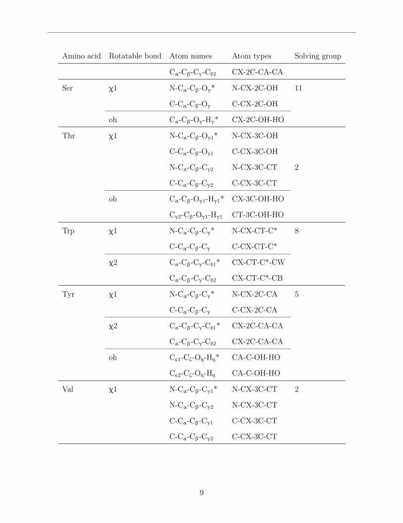
Table S1: The amino acids and the bonds that have been corrected, the four atom combi-nations, and the atom types of each correction that has been modified. This table has thesame contents as Table S2 on page 10, but sorted by amino acid.

Amino acid Rotatable bond Atom names Atom types Solving group

Arg χ1 N-Cα-Cβ-Cγ* N-CX-C8-C8 6

C-Cα-Cβ-Cγ C-CX-C8-C8

χ2 Cα-Cβ-Cγ-Cδ* CX-C8-C8-C8

χ3 Cβ-Cγ-Cδ-Nε* C8-C8-C8-N2

χ4 Cγ-Cδ-Nε-Cζ* C8-C8-N2-CA

Ash χ1 N-Cα-Cβ-Cγ* N-CX-2C-C 3

C-Cα-Cβ-Cγ C-CX-2C-C

χ2 Cα-Cβ-Cγ-Oδ1* CX-2C-C-O

Cα-Cβ-Cγ-Oδ2 CX-2C-C-OH

oh Cβ-Cγ-Oδ2-Hδ2* 2C-C-OH-HO

Asn χ1 N-Cα-Cβ-Cγ* N-CX-2C-C 3

C-Cα-Cβ-Cγ C-CX-2C-C

χ2 Cα-Cβ-Cγ-Oδ1* CX-2C-C-O

Cα-Cβ-Cγ-Nδ2 CX-2C-C-N

Asp χ1 N-Cα-Cβ-Cγ* N-CX-2C-CO 9

C-Cα-Cβ-Cγ C-CX-2C-CO

χ2 Cα-Cβ-Cγ-Oδ1* CX-CS-CO-O2

Cα-Cβ-Cγ-Oδ2 CX-CS-CO-O2

Cys χ1 N-Cα-Cβ-Sγ* N-CX-2C-SH 7

C-Cα-Cβ-Sγ C-CX-2C-SH

χ2 Cα-Cβ-Sγ-Hγ* CX-2C-SH-HS

Cyx χ1 N-Cα-Cβ-Sγ* N-CX-2C-S 0

C-Cα-Cβ-Sγ C-CX-2C-S

6


χ2 Cα-Cβ-Sγ-Sγ′* CX-2C-S-S

χSS Cβ-Sγ-Sγ′-Cβ′* 2C-S-S-2C

Glh χ1 N-Cα-Cβ-Cγ* N-CX-2C-2C 1

C-Cα-Cβ-Cγ C-CX-2C-2C

χ2 Cα-Cβ-Cγ-Cδ* CX-2C-2C-C

χ3 Cβ-Cγ-Cδ-Oε1* 2C-2C-C-OH

Cβ-Cγ-Cδ-Oε2 2C-2C-C-OH

Gln χ1 N-Cα-Cβ-Cγ* N-CX-2C-2C 1


χ2 Cα-Cβ-Cγ-Cδ* CX-2C-2C-C

χ3 Cβ-Cγ-Cδ-Oε1* 2C-2C-C-O

Cβ-Cγ-Cδ-Nε2 2C-2C-C-N

Glu χ1 N-Cα-Cβ-Cγ* N-CX-2C-2C 1


χ2 Cα-Cβ-Cγ-Cδ* CX-2C-2C-CO

χ3 Cβ-Cγ-Cδ-Oε1* 2C-2C-C-O2

Cβ-Cγ-Cδ-Oε2 2C-2C-C-O2

Hid χ1 N-Cα-Cβ-Cγ* N-CX-CT-CC 4

C-Cα-Cβ-Cγ C-CX-CT-CC

χ2 Cα-Cβ-Cγ-Nδ1* CX-CT-CC-NA

Cα-Cβ-Cγ-Cδ2 CX-CT-CC-CV

Hie χ1 N-Cα-Cβ-Cγ* N-CX-CT-CC 4


χ2 Cα-Cβ-Cγ-Nδ1* CX-CT-CC-NB

Cα-Cβ-Cγ-Cδ2 CX-CT-CC-CW

Hip χ1 N-Cα-Cβ-Cγ* N-CX-CT-CC 4

7



χ2 Cα-Cβ-Cγ-Nδ1* CX-CT-CC-NA

Cα-Cβ-Cγ-Cδ2 CX-CT-CC-CW

Ile χ1 N-Cα-Cβ-Cγ1* N-CX-3C-2C

C-Cα-Cβ-Cγ1 C-CX-3C-2C

N-Cα-Cβ-Cγ2 N-CX-3C-CT 2

C-Cα-Cβ-Cγ2 C-CX-3C-CT

χ2 Cα-Cβ-Cγ1-Cδ1* CX-3C-2C-CT

Cγ2-Cβ-Cγ1-Cδ1 CT-3C-2C-CT

Leu χ1 N-Cα-Cβ-Cγ* N-CX-2C-3C 10


χ2 Cα-Cβ-Cγ-Cδ1* CX-CS-3C-CT

Cα-Cβ-Cγ-Cδ2 CX-CS-3C-CT

Lys χ1 N-Cα-Cβ-Cγ* N-CX-C8-C8 6

C-Cα-Cβ-Cγ C-CX-C8-C8

χ2 Cα-Cβ-Cγ-Cδ* CX-C8-C8-C8

χ3 Cβ-Cγ-Cδ-Cε* C8-C8-C8-C8

χ4 Cγ-Cδ-Cε-Nζ* C8-C8-C8-N3

Met χ1 N-Cα-Cβ-Cγ* N-CX-2C-2C 1


χ2 Cα-Cβ-Cγ-Sδ* CX-2C-2C-S

χ3 Cβ-Cγ-Sδ-Cε* 2C-2C-S-CT

Phe χ1 N-Cα-Cβ-Cγ* N-CX-2C-CA 5

C-Cα-Cβ-Cγ C-CX-2C-CA

χ2 Cα-Cβ-Cγ-Cδ1* CX-2C-CA-CA

8


Cα-Cβ-Cγ-Cδ2 CX-2C-CA-CA

Ser χ1 N-Cα-Cβ-Oγ* N-CX-2C-OH 11

C-Cα-Cβ-Oγ C-CX-2C-OH

oh Cα-Cβ-Oγ-Hγ* CX-2C-OH-HO

Thr χ1 N-Cα-Cβ-Oγ1* N-CX-3C-OH

C-Cα-Cβ-Oγ1 C-CX-3C-OH

N-Cα-Cβ-Cγ2 N-CX-3C-CT 2


oh Cα-Cβ-Oγ1-Hγ1* CX-3C-OH-HO

Cγ2-Cβ-Oγ1-Hγ1 CT-3C-OH-HO

Trp χ1 N-Cα-Cβ-Cγ* N-CX-CT-C* 8

C-Cα-Cβ-Cγ C-CX-CT-C*

χ2 Cα-Cβ-Cγ-Cδ1* CX-CT-C*-CW

Cα-Cβ-Cγ-Cδ2 CX-CT-C*-CB

Tyr χ1 N-Cα-Cβ-Cγ* N-CX-2C-CA 5

C-Cα-Cβ-Cγ C-CX-2C-CA

χ2 Cα-Cβ-Cγ-Cδ1* CX-2C-CA-CA

Cα-Cβ-Cγ-Cδ2 CX-2C-CA-CA

oh Cε1-Cζ-Oη-Hη* CA-C-OH-HO

Cε2-Cζ-Oη-Hη CA-C-OH-HO

Val χ1 N-Cα-Cβ-Cγ1* N-CX-3C-CT 2

N-Cα-Cβ-Cγ2 N-CX-3C-CT



9

Table S2: The atom types of each correction modified, the residues, bonds, and 4-atom namecombinations affected

Dihedral atom types Rotamers affected Dihedral atom names

N-CX-C8-C8 Arg χ1 N-Cα-Cβ-Cγ

Lys χ1

C-CX-C8-C8 Arg χ1 C-Cα-Cβ-Cγ

Lys χ1

CX-C8-C8-C8 Arg χ2 Cα-Cβ-Cγ-Cδ

Lys χ2

C8-C8-C8-C8 Lys χ3 Cβ-Cγ-Cδ-Cε

C8-C8-C8-N3 Lys χ4 Cγ-Cδ-Cε-Nζ

C8-C8-C8-N2 Arg χ3 Cβ-Cγ-Cδ-Nε

C8-C8-N2-CA Arg χ4 Cγ-Cδ-Nε-Cζ

N-CX-2C-SH Cys χ1 N-Cα-Cβ-Sγ

C-CX-2C-SH Cys χ1 C-Cα-Cβ-Sγ

CX-2C-SH-HS Cys χ2 Cα-Cβ-Sγ-Hγ

N-CX-2C-S Cyx χ1 N-Cα-Cβ-Sγ

C-CX-2C-S Cyx χ1 C-Cα-Cβ-Sγ

CX-2C-S-S Cyx χ2 Cα-Cβ-Sγ-Sγ′

2C-S-S-2C Cyx χSS Cβ-Sγ-Sγ′-Cβ′

N-CX-CT-C* Trp χ1 N-Cα-Cβ-Cγ

C-CX-CT-C* Trp χ1 C-Cα-Cβ-Cγ

CX-CT-C*-CW Trp χ2 Cα-Cβ-Cγ-Cδ1

CX-CT-C*-CB Trp χ2 Cα-Cβ-Cγ-Cδ2

N-CX-2C-CO Asp χ1 N-Cα-Cβ-Cγ

C-CX-2C-CO Asp χ1 C-Cα-Cβ-Cγ

CX-CS-CO-O2 Asp χ2 Cα-Cβ-Cγ-Oδ1

10


Cα-Cβ-Cγ-Oδ2

N-CX-2C-C Ash χ1 N-Cα-Cβ-Cγ

Asn χ1

C-CX-2C-C Ash χ1 C-Cα-Cβ-Cγ

Asn χ1

CX-2C-C-O Ash χ2 Cα-Cβ-Cγ-Oδ1

Asn χ2

CX-2C-C-OH Ash χ2 Cα-Cβ-Cγ-Oδ2

CX-2C-C-N Asn χ2 Cα-Cβ-Cγ-Nδ2

N-CX-2C-OH Ser χ1 N-Cα-Cβ-Oγ

C-CX-2C-OH Ser χ1 C-Cα-Cβ-Oγ

CX-2C-OH-HO Ser oh Cα-Cβ-Oγ-Hγ

N-CX-2C-3C Leu χ1 N-Cα-Cβ-Cγ

C-CX-2C-3C Leu χ1 C-Cα-Cβ-Cγ

CX-CS-3C-CT Leu χ2 Cα-Cβ-Cγ-Cδ1

Cα-Cβ-Cγ-Cδ2

N-CX-3C-CT Ile χ1 N-Cα-Cβ-Cγ2

Thr χ1

Val χ1 N-Cα-Cβ-Cγ1

N-Cα-Cβ-Cγ2

C-CX-3C-CT Ile χ1 C-Cα-Cβ-Cγ2

Thr χ1

Val χ1 C-Cα-Cβ-Cγ1

C-Cα-Cβ-Cγ2

N-CX-3C-2C Ile χ1 N-Cα-Cβ-Cγ1

11


C-CX-3C-2C Ile χ1 C-Cα-Cβ-Cγ1

N-CX-3C-OH Thr χ1 N-Cα-Cβ-Oγ1

C-CX-3C-OH Thr χ1 C-Cα-Cβ-Oγ1

CX-3C-2C-CT Ile χ2 Cα-Cβ-Cγ1-Cδ1

CT-3C-2C-CT Ile χ2 Cγ2-Cβ-Cγ1-Cδ1

CX-3C-OH-HO Thr oh Cα-Cβ-Oγ1-Hγ1

N-CX-2C-CA Phe χ1 N-Cα-Cβ-Cγ

Tyr χ1

C-CX-2C-CA Phe χ1 C-Cα-Cβ-Cγ

Tyr χ1

CX-2C-CA-CA Phe χ2 Cα-Cβ-Cγ-Cδ1

Tyr χ2 Cα-Cβ-Cγ-Cδ2

CA-C-OH-HO Tyr oh Cε1-Cζ-Oη-Hη

Cε2-Cζ-Oη-Hη

N-CX-CT-CC Hid χ1 N-Cα-Cβ-Cγ

Hie χ1

Hip χ1

C-CX-CT-CC Hid χ1 C-Cα-Cβ-Cγ

Hie χ1

Hip χ1

CX-CT-CC-NA Hid χ2 Cα-Cβ-Cγ-Nδ1

Hip χ2

CX-CT-CC-NB Hie χ2 Cα-Cβ-Cγ-Nδ1

CX-CT-CC-CV Hid χ2 Cα-Cβ-Cγ-Cδ2

CX-CT-CC-CW Hie χ2 Cα-Cβ-Cγ-Cδ2

12


Hip χ2

N-CX-2C-2C Glh χ1 N-Cα-Cβ-Cγ

Gln χ1

Glu χ1

Met χ1

C-CX-2C-2C Glh χ1 C-Cα-Cβ-Cγ

Gln χ1

Glu χ1

Met χ1

CX-2C-2C-C Glh χ2 Cα-Cβ-Cγ-Cδ

Gln χ2

2C-2C-C-OH Glh χ3 Cβ-Cγ-Cδ-Oε2

2C-2C-C-N Gln χ3 Cβ-Cγ-Cδ-Nε2

CX-2C-2C-CO Glu χ2 Cα-Cβ-Cγ-Cδ

2C-2C-C-O2 Glu χ3 Cβ-Cγ-Cδ-Oε1

Cβ-Cγ-Cδ-Oε2

CX-2C-2C-S Met χ2 Cα-Cβ-Cγ-Sδ

2C-2C-S-CT Met χ3 Cβ-Cγ-Sδ-Cε

13

Table S3: Objective values O for each of the solving groups

Solving group Amino acids Off99SB Off14SB # params # structures # pairs0 Cyx 1.5 1.2 20 1548 784 4941 Glh Gln Glu Met 1.6 1.1 39 2986 587 6992 Ile Thr Val 1.2 0.8 52 1368 210 5643 Ash Asn 2.0 1.1 25 1800 435 8524 Hid Hie Hip 1.3 1.0 24 1944 313 9565 Phe Tyr 1.7 0.8 20 1224 187 3086 Arg Lys 1.5 1.1 28 1656 345 5317 Cys 1.3 1.0 16 648 104 6528 Trp 1.3 1.0 20 648 104 6529 Asp 2.5 0.9 16 648 104 652

10 Leu 1.2 0.9 16 648 104 65211 Ser 1.4 0.9 16 648 104 652

Table S4: Distribution of REEs in terms of mean, standard deviation (stdev), minimum(min), and maximum (max), for ff99SB or ff14SB side chain parameters, against the confor-mations of each amino acid (AA) and backbone conformation (BB). ‘# confs’ is the numberof conformations in each set.

ff99SB ff14SB

AA BB#

confsmean stdev min max mean stdev min max

Arg α 396 1.41 1.07 0.00 6.97 1.06 0.86 0.00 7.87

Arg β 355 1.50 1.23 0.00 8.71 1.06 0.96 0.00 8.10

Ash α 576 1.87 1.44 0.00 10.51 1.22 0.96 0.00 7.76

Ash β 576 2.06 1.55 0.00 10.71 0.96 0.78 0.00 7.21

Asn α 324 1.99 1.50 0.00 8.70 1.06 0.79 0.00 4.86

Asn β 324 1.97 1.44 0.00 9.02 0.97 0.73 0.00 4.62

Asp α 324 2.63 1.95 0.00 10.65 1.11 0.85 0.00 4.63

Asp β 324 2.46 1.76 0.00 8.76 0.73 0.68 0.00 4.43

Cys α 324 1.42 1.17 0.00 7.11 1.14 1.02 0.00 5.43

Cys β 324 1.15 0.84 0.00 5.14 0.91 0.68 0.00 3.95

Glh α 436 1.63 1.25 0.00 9.29 1.23 1.01 0.00 7.53

14

ff99SB ff14SB

AA BB#


Glh β 420 1.48 1.11 0.00 7.14 0.92 0.73 0.00 4.88

Gln α 313 1.69 1.30 0.00 8.18 1.23 0.92 0.00 6.49

Gln β 282 1.29 1.03 0.00 7.01 0.91 0.70 0.00 4.52

Glu α 284 1.96 1.48 0.00 7.62 1.26 0.97 0.00 5.95

Glu β 271 2.03 1.52 0.00 8.40 1.29 1.00 0.00 6.31

Hid α 324 1.09 0.83 0.00 5.52 0.76 0.56 0.00 3.71

Hid β 324 1.24 0.99 0.00 6.66 0.79 0.65 0.00 4.14

Hie α 324 1.24 0.99 0.00 7.51 0.92 0.69 0.00 4.52

Hie β 324 1.37 1.00 0.00 6.11 0.99 0.72 0.00 3.98

Hip α 324 1.55 1.18 0.00 6.24 1.46 1.08 0.00 6.24

Hip β 324 1.36 1.03 0.00 7.02 1.04 0.82 0.00 6.45

Ile α 324 1.64 1.20 0.00 6.60 0.97 0.73 0.00 4.62

Ile β 324 1.17 0.87 0.00 5.40 0.77 0.58 0.00 3.42

Leu α 324 1.19 0.87 0.00 4.86 1.01 0.78 0.00 4.45

Leu β 324 1.28 0.93 0.00 4.87 0.76 0.56 0.00 3.30

Lys α 466 1.66 1.34 0.00 8.07 1.30 1.08 0.00 7.80

Lys β 439 1.38 1.09 0.00 8.07 0.96 0.79 0.00 6.17

Met α 483 1.33 1.10 0.00 8.01 1.16 0.96 0.00 7.30

Met β 497 1.22 1.01 0.00 7.96 1.02 0.85 0.00 6.82

Phe α 324 0.86 0.70 0.00 4.47 0.88 0.67 0.00 4.24

Phe β 324 0.98 0.75 0.00 4.08 0.77 0.60 0.00 3.56

Ser α 324 1.68 1.26 0.00 7.67 1.01 0.75 0.00 4.50

Ser β 324 1.17 0.88 0.00 5.00 0.71 0.53 0.00 3.04

Thr α 324 1.58 1.16 0.00 6.37 0.92 0.73 0.00 4.14

15

ff99SB ff14SB

AA BB#


Thr β 324 1.22 0.89 0.00 5.00 0.81 0.63 0.00 3.51

Trp α 324 1.37 1.15 0.00 9.76 1.13 1.12 0.00 11.54

Trp β 324 1.25 1.02 0.00 8.26 0.91 0.95 0.00 8.81

Tyr α 288 2.44 1.92 0.00 8.63 0.83 0.62 0.00 3.82

Tyr β 288 2.45 1.92 0.00 8.85 0.73 0.55 0.00 3.43

Val α 36 1.17 0.86 0.00 3.37 0.77 0.58 0.00 2.77

Val β 36 0.53 0.37 0.00 1.44 0.36 0.32 0.00 1.08

16

Alanine dipeptide PMFs

Figure S1: PMFs of alanine dipeptide in TIP3P water simulated with A) ff99SB, B) mod1φ,C) mod1φ2ψ, and D) mod3φ.

Defining EQM and EMM

Ideally, one should start with relatively close agreement between ff99SB and

MP2/6-31+G**//HF/6-31G* energies (low AAE), with similar errors between different

backbone conformations (low BBD), if dihedral parameters are to reconcile errors with-

out explicit coupling to the backbone conformation. According to the penultimate rotamer

library7, the side chains of aspartate and asparagine depend most on backbone conforma-

tion; we thus chose them for initial testing of how the energy calculations impact coupling

17

between side chain and backbone dihedral parameters.

Restraining all backbone dihedrals and re-optimizing the QM structure with MM be-

fore calculating energy yielded both the lowest AAE (2.55± 0.09 kcal mol−1 for Asp and

1.98± 0.01 kcal mol−1 for Asn, error bars reflect difference between α and β backbone con-

text) and lowest BBD (1.35± 0.01 kcal mol−1 for Asp and 1.42± 0.03 kcal mol−1 for Asn,

error bars reflect difference between two staggered halves of structures), as shown in Fig-

ure S2 on the following page. At the opposite extreme, restraining just φ and ψ and using the

QM structures to calculate MM energies resulted in the greatest AAE (3.45±0.13 kcal mol−1

for Asp and 3.09 ± 0.74 kcal mol−1 for Asn) and BBD (2.23± 0.02 kcal mol−1 for Asp and

3.90± 0.08 kcal mol−1 for Asn). Fundamental differences in the modeling of bonded and non-

bonded interactions between QM and MM are likely exacerbated when the QM-optimized

structures are evaluated in MM without re-optimization; these differences manifest as larger

errors in MM energy, as well as less transferability between backbone contexts. Restraining

all possible combinations of four-atoms describing each dihedral in both the backbone and

side chain was also attempted (this approach led to the ff12SB parameter set, see Section

on page 42), but restraining all 4-atom dihedrals in the side chains prevented relaxation of

angle terms in MM optimization, leading to increased error that likely would not be present

in a simulation when steric clashes can be alleviated through adjustment of covalent struc-

ture. Based on these results, we made the decision to restrain all backbone dihedrals during

structure optimization, but only the defining dihedrals for side chains, and to re-optimize the

QM structures with the MM model (using the same restraints) prior to calculation of MM

energies. These energies were used in the calculation of the objective function in Equation

(6).

18

Figure S2: AAE vs. BBD of aspartate and asparagine, calculating MM energies of QMstructures and restraining: φ and ψ (red crosses) or all backbone dihedrals (blue stars); orcalculating MM energies of MM re-optimized structures and restraining: φ and ψ (green‘X’s) or all backbone dihedrals (purple squares). The latter provides the lowest AAE values,as well as the best intrinsic transferability between backbone conformations. Error bars inAAE indicate difference between AAE calculated in the α or β backbone context, and BBDusing half of the structures.

19

Backbone modification

We changed the backbone potential to enhance helical sampling and scalar couplings8 in

Ala5. To be sure we corrected the appropriate backbone potential or combination of backbone

potentials, we perturbed φ and ψ backbone potentials and then combined all pairs of φ and

ψ potentials.

Modifications to φ potentials targeted both scalar coupling deviations and helical sam-

pling. Too high HN-H scalar couplings suggest too many structures near φ = −120◦, where

this scalar coupling is maximal. This transition was destabilized by increasing the n = 3 φ′

amplitude from 0.4 kcal/mol to 0.6 kcal/mol or 0.8 kcal/mol, modifications (mods) referred

to as 3φ and 4φ, respectively. Not enough helical content, particularly ppII, also suggests

that helices are not stable enough relative to strands. Helices were stabilized by decreasing

the n = 2 φ′ amplitude from 2 kcal/mol to 1.8 kcal/mol, yielding mod1φ and 2φ when added

to mod3φ and 4φ, respectively.

As another work suggested that helical undersampling results from errors in ψ, not φ,

we also explored several ψ corrections. Two simply stabilize α relative to β and ppII. The

first stabilizes ψ in the vicinity of −45◦ to −40◦ by increasing the ψ′ n = 1 amplitude

from 0.2 kcal/mol to 0.3 kcal/mol and phase shifting by −60◦, denoted by 4ψ. The second

favors structures centered on the eclipsed ψ of 0◦ by increasing the n = 1 ψ amplitude from

0.45 kcal/mol to 0.6 kcal/mol or 0.7 kcal/mol, the former of which constitutes modification

3ψ. Modification 2ψ was formed from mod3ψ by making structures centered around ψ of

±45◦ and ±135◦ more favorable by introducing a ψ′ n = 4 term with amplitude 0.4 kcal/mol

and phase shift of 120◦. Starting with this change together with the 0.7 kcal/mol amplitude

variation of the second basic ψ correction, we stabilized structures near ψ of −30◦ and 150◦

and destabilized structures near −120◦ and 60◦, increasing the barriers, by increasing the ψ′

n = 2 amplitude from 0.2 kcal/mol to 0.5 kcal/mol, this conglomerate referred to as mod1ψ.

Each of the φ variants was then combined with each of the ψ variants, including ff99SB

φ and ψ corrections. Thus we formed 24 ff99SB variants to evaluate which works best.

20

Table S5: Revisions to φ′

Correction termForce field V 1′/2 V 2′/2 V 3′/2

ff99SB 2.0 2.0 0.4mod1φ 2.0 1.8 0.8mod2φ 2.0 1.8 0.6mod3φ 2.0 2.0 0.8mod4φ 2.0 2.0 0.6mod5φ 1.8 2.0 0.8

ff99SB and candidate changes to the φ′ correction mod1-5φ. Phase shift is 0◦. Parameterschanged from ff99SB are colored blue.

Table S6: Revisions to ψ(′)

Force fieldCorrection term ff99SB mod1ψ mod2ψ mod3ψ mod4ψ

V 1/2 -0.45 -0.70 -0.60 -0.60 -0.45V 2/2 -1.58 -1.58 -1.58 -1.58 -1.58V 3/2 -0.55 -0.55 -0.55 -0.55 -0.55V 1′/2 0.20 0.20 0.20 0.20 0.30a

V 2′/2 0.20 0.50 0.20 0.20 0.20V 3′/2 0.40 0.40 0.40 0.40 0.40V 4′/2 0 0.40b 0.40b 0 0

a. Phase shift of −60◦

b. Phase shift of 120◦

ff99SB and candidate changes to ψ and ψ′ corrections. Negative amplitude indicates phaseshift of 180◦. The mod4ψ ψ′ n = 1 correction has a phase shift of −60◦. The mod1ψ andmod2ψ ψ′ n = 4 corrections have a phase shift of 120◦. Parameters changed from ff99SB

are colored blue.

21

Building hydrogen bond surrogate peptide

We restrained the hydrogen bond between the Ac1:CO and the A5:HN. Two criteria were

used to identify an appropriate Ac1:O - A5:HN restraint distance. First, the PDB was sur-

veyed for proteins whose structure was determined by X-ray crystallography at a resolution

of <0.9 A, to provide hydrogen atom positions. Next, we looked at those proteins which had

an α-helix length of 40–50 amino acids so that a large number of backbone helical hydro-

gen bonds would be present. One suitable structure was found satisfying these two criteria,

Pichia pastoris aquaporin Aqy1 (PDB ID: 3ZOJ),9 which was resolved at 0.88 A and had 106

backbone helical hydrogen bonds. We histogrammed the length of all the backbone α-helical

hydrogen bonds. The peak of the histogram of these distances was observed at 2.03 A. To

find the optimal weight for restraining the Ac1:O - A5:HN bond distance, test simulations

were run for 160.0 ns using ff99SB10 using different weights and the histogram of the Ac1:O

- A5:HN distance was plotted (Figure S3 on the following page). Using a restraint weight

of 100.0 kcal/mol/A2 provides a peak at 2.03 A with similar distribution to that found in

3ZOJ, and hence, was used for production runs. The authors note that the distribution is

likely narrower for a crystal structure than expected from room-temperature dynamics; as

the goal is to emulate a covalent bond, referring to a crystal structure may be reasonable.

22

Figure S3: The Ac1:O - A5:HN distance probability distribution using different weights.The units of the weights are in kcal/mol/A2. The distribution of hydrogen bond distancesobserved in 3ZOJ is shown in gray.

23

Additional testing analysis

K19 per-residue helicity analysis

Figure S4: The helicity of each residue in K19, according to ff99SB (gray), mod1φ (red),mod1φ2ψ, mod3φ, and CSDs11 (black). The force field helicity was determined from φ/ψangles, as described in the Methods section of the main text. The mod1φ simulations are inbest agreement with experimental CSDs.11

CLN025

Table S7: Sum of the NOE violations from the restraints determined in Ref 12 for CLN025,for each simulation using ff14SB and ff99SB starting from linear and native conformations.*FF=force field

aaaaaaaaFF*

run linear native1 2 3 4 1 2 3 4

ff14SB 3.6 1.8 3.7 2.4 2.1 1.8 1.5 2.1ff99SB 2.4 3.8 3.3 2.7 3.3 1.8 2.5 4.9

24

Figure S5: Licorice structures of CLN025. The NMR structure closest to the ensembleaverage,12 colored by atom (A); the centroid of cluster 0, the native-like cluster, colored black(B); the centroid of cluster 1, where a shift in hydrogen bonding accompanies extension ofthe C-terminus of the second strand past the N-terminus of the first strand and flipping ofW9 to the opposite side of the hairpin from Y2, against which it stacks in the NMR structureand cluster 0, and P4, which stacks against Y2, colored blue (C). Large licorice indicatesatoms used in the clustering mask; smaller licorice atoms were omitted from clustering.

25

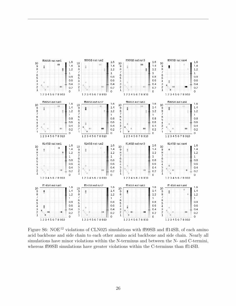
Figure S6: NOE12 violations of CLN025 simulations with ff99SB and ff14SB, of each aminoacid backbone and side chain to each other amino acid backbone and side chain. Nearly allsimulations have minor violations within the N-terminus and between the N- and C-termini,whereas ff99SB simulations have greater violations within the C-terminus than ff14SB.

26

Protein backbone RMSDs

Figure S7: GB3 backbone (N, Cα, C) RMSD to 1P7E13 for four runs of ff99SB (top row),ff99SB-ILDN (second row), ff14SBonlysc (third row), and ff14SB (fourth row). The proba-bility density function (pdf) and cumulative distribution function (cdf) are plotted for eachforce field in the bottom row.

27

Figure S8: BPTI backbone (N, Cα, C) RMSD to 5PTI14 for four runs of ff99SB (toprow), ff99SB-ILDN (second row), ff14SBonlysc (third row), and ff14SB (fourth row). Theprobability density function (pdf) and cumulative distribution function (cdf) are plotted foreach force field in the bottom row.

28

Figure S9: Ubiquitin backbone (N, Cα, C) RMSD to 1UBQ15 for four runs of ff99SB (toprow), ff99SB-ILDN (second row), ff14SBonlysc (third row), and ff14SB (fourth row). Theprobability density function (pdf) and cumulative distribution function (cdf) are plotted foreach force field in the bottom row.

29

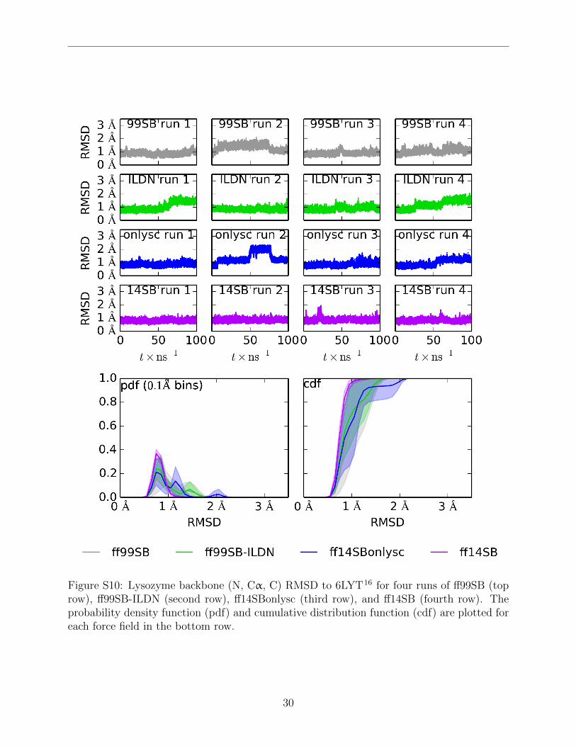
Figure S10: Lysozyme backbone (N, Cα, C) RMSD to 6LYT16 for four runs of ff99SB (toprow), ff99SB-ILDN (second row), ff14SBonlysc (third row), and ff14SB (fourth row). Theprobability density function (pdf) and cumulative distribution function (cdf) are plotted foreach force field in the bottom row.

30

Protein ramachandran histograms

-90°

90°

Gln2 Tyr3 Lys4 Leu5 Val6 Ile7 Asn8 Gly9 Lys10

-90°

90°

Thr11 Leu12 Lys13 Gly14 Glu15 Thr16 Thr17 Thr18 Lys19 Ala20

-90°

90°

Val21 Asp22 Ala23 Glu24 Thr25 Ala26 Glu27 Lys28 Ala29 Phe30

-90°

90°

Lys31 Gln32 Tyr33 Ala34 Asn35 Asp36 Asn37 Gly38 Val39 Asp40

-90°

90°

Gly41 Val42 Trp43 Thr44 Tyr45 Asp46 Asp47 Ala48 Thr49 Lys50

-90° 90°

-90°

90°

Thr51

-90° 90°

Phe52

-90° 90°

Thr53

-90° 90°

Val54

-90° 90°

Thr55

-90° 90° -90° 90° -90° 90° -90° 90° -90° 90°

Figure S11: Ramachandran histograms of each residue in GB3 from four simulations eachwith ff99SB (red) and ff14SB (blue)

31

-90°

90°

Pro2 Asp3 Phe4 Cyx5 Leu6 Glu7 Pro8 Pro9 Tyr10

-90°

90°

Thr11 Gly12 Pro13 Cyx14 Lys15 Ala16 Arg17 Ile18 Ile19 Arg20

-90°

90°

Tyr21 Phe22 Tyr23 Asn24 Ala25 Lys26 Ala27 Gly28 Leu29 Cyx30

-90°

90°

Gln31 Thr32 Phe33 Val34 Tyr35 Gly36 Gly37 Cyx38 Arg39 Ala40

-90°

90°

Lys41 Arg42 Asn43 Asn44 Phe45 Lys46 Ser47 Ala48 Glu49 Asp50

-90° 90°

-90°

90°

Cyx51

-90° 90°

Met52

-90° 90°

Arg53

-90° 90°

Thr54

-90° 90°

Cyx55

-90° 90°

Gly56

-90° 90°

Gly57

-90° 90° -90° 90° -90° 90°

Figure S12: Ramachandran histograms of each residue in bovine pancreatic trypsin inhibitorfrom four simulations each with ff99SB (red) and ff14SB (blue)

32

-90°

90°

Gln2 Ile3 Phe4 Val5 Lys6 Thr7 Leu8 Thr9 Gly10

-90°

90°

Lys11 Thr12 Ile13 Thr14 Leu15 Glu16 Val17 Glu18 Pro19 Ser20

-90°

90°

Asp21 Thr22 Ile23 Glu24 Asn25 Val26 Lys27 Ala28 Lys29 Ile30

-90°

90°

Gln31 Asp32 Lys33 Glu34 Gly35 Ile36 Pro37 Pro38 Asp39 Gln40

-90°

90°

Gln41 Arg42 Leu43 Ile44 Phe45 Ala46 Gly47 Lys48 Gln49 Leu50

-90°

90°

Glu51 Asp52 Gly53 Arg54 Thr55 Leu56 Ser57 Asp58 Tyr59 Asn60

-90°

90°

Ile61 Gln62 Lys63 Glu64 Ser65 Thr66 Leu67 Hip68 Leu69 Val70

-90° 90°

-90°

90°

Leu71

-90° 90°

Arg72

-90° 90°

Leu73

-90° 90°

Arg74

-90° 90°

Gly75

-90° 90° -90° 90° -90° 90° -90° 90° -90° 90°

Figure S13: Ramachandran histograms of each residue in ubiquitin from four simulationseach with ff99SB (red) and ff14SB (blue)

33

-90°

90°

Val2 Phe3 Gly4 Arg5 Cyx6 Glu7 Leu8 Ala9 Ala10

-90°

90°

Ala11 Met12 Lys13 Arg14 Hip15 Gly16 Leu17 Asp18 Asn19 Tyr20

-90°

90°

Arg21 Gly22 Tyr23 Ser24 Leu25 Gly26 Asn27 Trp28 Val29 Cyx30

-90°

90°

Ala31 Ala32 Lys33 Phe34 Glu35 Ser36 Asn37 Phe38 Asn39 Thr40

-90°

90°

Gln41 Ala42 Thr43 Asn44 Arg45 Asn46 Thr47 Asp48 Gly49 Ser50

-90°

90°

Thr51 Asp52 Tyr53 Gly54 Ile55 Leu56 Gln57 Ile58 Asn59 Ser60

-90°

90°

Arg61 Trp62 Trp63 Cyx64 Asn65 Asp66 Gly67 Arg68 Thr69 Pro70

-90°

90°

Gly71 Ser72 Arg73 Asn74 Leu75 Cyx76 Asn77 Ile78 Pro79 Cyx80

-90°

90°

Ser81 Ala82 Leu83 Leu84 Ser85 Ser86 Asp87 Ile88 Thr89 Ala90

-90° 90°

-90°

90°

Ser91

-90° 90°

Val92

-90° 90°

Asn93

-90° 90°

Cyx94

-90° 90°

Ala95

-90° 90°

Lys96

-90° 90°

Lys97

-90° 90°

Ile98

-90° 90°

Val99

-90° 90°

Ser100

Figure S14: Ramachandran histograms of each residue in lysozyme from four simulationseach with ff99SB (red) and ff14SB (blue), for residues 2 to 100.

34

-90°

90°

Asp101 Gly102 Asn103 Gly104 Met105 Asn106 Ala107 Trp108 Val109 Ala110

-90°

90°

Trp111 Arg112 Asn113 Arg114 Cyx115 Lys116 Gly117 Thr118 Asp119 Val120

-90° 90°

-90°

90°

Gln121

-90° 90°

Ala122

-90° 90°

Trp123

-90° 90°

Ile124

-90° 90°

Arg125

-90° 90°

Gly126

-90° 90°

Cyx127

-90° 90°

Arg128

-90° 90° -90° 90°

Figure S15: Ramachandran histograms of each residue in lysozyme from four simulationseach with ff99SB (red) and ff14SB (blue), for residues 101 to 128.

Significance analysis

One way to incorporate statistical significance into analyzing force field differences is to plot

the average difference in errors for all scalar couplings whose comparison satisfies any of a

range of p-values. Those that satisfy lower p-values may be considered more informative

than those that only satisfy higher p-values. The probability that distributions are not

different was approximated by Welch’s t-test17. The p-value was calculated using the survival

function of the SciPy18,19 stats module, based on t as in Equation (2) with µFF and SEFF

corresponding to the average normalized error and standard error of the mean normalized

error, respectively, for each force field FF , and degrees of freedom approximated by the

Welch-Satterthwaite equation17,20, (Equation (3); n1, being 3 for all force fields, enters the

numerator).

t = (µff14SB − µff99SB−ILDN)(SE 2

ff14SB − SE 2ff99SB−ILDN

)− 12 (2)

d .f . =3(SE 2

ff14SB + SE 2ff99SB−ILDN

)2)

SE 4ff14SB + SE 4

ff99SB−ILDN

(3)

35

Figure S16: Left column: all average normalized errors (ANE, defined in main text) accordingto ff99SB-ILDN21 (x-axis) and ff14SB (y-axis). Middle column: a subset of the errors wherethe uncertainties do not cross the equivalence line. Right column: the average difference innormalized error from ff99SB-ILDN to ff14SB (y-axis) for normalized errors with significanceof p < P (x-axis). Top row: GB3 (A-C). Second row: ubiquitin (D-F). Third row: lysozyme(G-I). Bottom row: BPTI (J-L).

36

Backbone dependence

As ubiquitin D32 was the most statistically different between the two force fields, we at-

tempted to decompose its simulation accuracy according to fitting method, potentially pro-

viding insight to guide future parameter optimization efforts. First, we used ff14SB aspartate

side chain parameters in ff99SB-ILDN to ensure that aspartate side chain parameters are

responsible for observed differences. This significantly reduced the D32 ANE to a value com-

parable to ff14SB (0.077± 0.006), confirming direct influence of the Asp parameters on D32

dynamics. The most obvious methodological difference that could explain this phenomenon

is the inclusion of helical backbone structures in training. We repeated the optimization

for solving group 10 (containing just aspartate), but using only β backbone conformations

in Equation (5). Simulations using these parameters still resulted in rather low ANE of

0.070± 0.008, suggesting that this particular improvement was not due to inclusion of fit-

ting for both backbone conformations. A second possibility is that our fitting protocols

had several differences compared to ff99SB-ILDN, such as weighting of squared QM-MM

energy differences by QM energy in the ff99SB-ILDN fitting, which could introduce bias if

positions of side chain rotamer minima are coupled to backbone conformation. Another pro-

tocol difference is that ff14SB parameters used two 4-atom dihedrals to describe χ1, while

ff99SB-ILDN fit only one set. We refit parameters for solving group 10 using the ff14SB

protocol but with the aspartate QM and MM energies published by Lindorff-Larsen et al. 21 .

With the resulting parameters, sampling of D32 was not improved compared to ff99SB-ILDN

(ANE = 0.42 ± 0.07), suggesting that the D32 performance is related to differences in the

QM benchmarks used to train the two force fields rather than the optimization protocol.

Although both data sets used a 2D scan of χ1 and χ2, the resulting energies are influenced

by the level of QM theory and the restraints used to generate potential energy surfaces for

fitting. To test the influence of restraints, we used the potential energy surfaces that we

generated with different structure optimization methods to test backbone-dependence (Fig-

ure 3). We therefore retrained solving group 10 parameters based on potential energy scans

37

of only β, or α and β conformations, using the combinations of restraints and QM or MM

optimized structures as carried out for Figure S2 on page 19. The ANE of D32, and of

all aspartates in ubiquitin, were plotted against the BBD of each method in Figure S17 on

the following page. For the parameters trained using only β dipeptides, the BBD of each

method forwardly predicts the error of D32 obtained using those parameters. This suggests

that how the structures in a potential energy surface are generated can significantly alter

their transferability. In fact, the combination matching ff99SB-ILDN (restraining only φ and

ψ, using QM structures for MM energies) also provided comparable results to ff99SB-ILDN

(ANE of 0.32± 0.11), suggesting that the deviation in MD from solvated protein NMR data

can be traced to the restraint method used during parameter development. The largest er-

rors arise when using QM structures for MM energies with fewer restraints; these errors are

reduced when both α and β dipeptides are used in fitting, perhaps because artifacts from

backbone interactions are lessened when requiring that the parameters work in multiple

backbone contexts (for example, D32 ANE is reduced from 0.32± 0.11 with β-only training

to 0.067± 0.007 using both α and β). Although we examined only one location in detail

(D32), the same trend holds when considering all Asp residues in ubiquitin (Figure S17 on

the next page). These results on agreement between MD and NMR also mirror the findings

in Figure S2 on page 19, where the ability to reproduce QM energies (AAE) showed a sim-

ilar dependence on BBD for different restraint methods. Taken together, the results show

not only the sensitivity of the model to restraint method, but also reinforce that improved

reproduction of gas-phase QM dipeptide energies leads to a better match to NMR data for

proteins simulations in water.

If we expand the backbone-dependent comparison to consider all ILDN residues within he-

lices versus all those without, we observe the same trends of ff14SB backbone-independence.

The average errors of all I, L, D, and N residues in helices were 0.18 ± 0.01 with ff99SB-

ILDN and 0.13± 0.01 with ff14SB. On the other hand, the average errors of all ILD and N

residues not in helices were 0.11 ± 0.01 with both force fields. This indicates that overall

38

Figure S17: Simulated average normalized error (ANE) of ubiquitin (Ubq) D32 and all Ubqaspartate (Asp), with parameters developed from β or α and β conformations of aspartatedipeptides with restraints on all backbone dihedrals (BB) or only φ and ψ (φψ), and withmolecular mechanics energies calculated for molecular mechanics structures (MM(MM)),or quantum mechanics structures (MM(QM)), versus backbone dependence on the x-axis.Parameters from β dipeptides with less backbone-dependent errors against quantum me-chanics also exhibit lower errors against helical D32 scalar couplings. Training with α and βconformations performs comparably or, as in MM(QM)/φψ, better against scalar couplings.

39

errors for side chains in helical context are improved with ff14SB relative to ff99SB-ILDN,

and that in ff14SB these errors are similar in magnitude to the non-helical side chain errors

for both force fields. It seems reasonable to conclude that this improved transferability in

ff14SB arises directly from the training of ff14SB against more transferable energy targets

than other options tested, with multiple backbone conformations.

Order parameter calculations using 2, 4, and 8 ns windows

In addition to the order parameter calculations reported in the main text, we calculated

order parameters for GB3, ubiqutin, and lysozyme using iRED22 with 2, 4, and 8 ns win-

dows, consistent with previous work by Li and Bruschweiler 23 (ubiquitin and lysozyme) and

Markwick et al. 24 (GB3). According to this analysis, all force fields are within 0.05 RMSD

of experimental S2, with subtle differences between them.

Several turns or loops increased in order with ff14SB. In the cases of loops L1 and L4 in

lysozyme, this increased order better reproduces experimental order parameters. Turn T3 in

GB3 and loop L3 in lysozyme, however, may have become too ordered although the differ-

ences are within precision errors. L3 begins with S85, which is 0.16± 0.04 too ordered. With

ff99SB, S85 was already 0.10± 0.02 too ordered, meanwhile D87 was 0.09± 0.02 too disor-

dered with ff99SB but only 0.05± 0.01 too ordered with ff14SB. Naturally, these estimates

depend on both the accuracy of the iRED method and the uncertainty in the simulations

and experiments; absolute comparisons against the experimental S2 differing by 0.06± 0.04

should not be overemphasized. But as a trend, there appears to be slightly less flexibility in

loops in ff14SB compared to ff99SB, both aiding and lessening agreement between iRED and

experimental order parameters. We conclude that ff14SB maintained ff99SB order parameter

reproduction on average, but with subtle reduction in flexibility.

40

Figure S18: Order parameters from NMR compared to those back calculated by iRED forff99SB, ff99SB-ILDN, and ff14SB simulations of GB3, ubiquitin, and lysozyme. Error barsrepresent the standard deviation of average values from four independent runs. The toppanels show differences between simulation and experiment, while the lowest panels showaverage data for each secondary structure region, following Hornak et al. 10 .

41

ff12SB

The ff12SB that was bundled with AMBER1225 differs from ff14SB presented here in three

ways. First, all four-atom dihedrals were frozen in the ff12SB training set structure mini-

mization. This was done to reduce the influence of conformations with strong electrostatic

interactions that resulted in different geometric distortions (e.g., in the amide planarity)

between the QM and MM structures. This helped reduce the effect of strong electrostatics

in residues like aspartate, but prevented covalent relaxation of steric clashes. By restraining

only one 4-atom set per side chain rotatable bond in the ff14SB training set, but continuing

to restrain all 4-atom sets in the backbone, the effect of electrostatic interactions was dimin-

ished while reducing the steric clashes in the training set, enabling a finer fit to quantum

energies and subsequently better agreement with experimental scalar couplings.

A second problem arose when fitting corrections for different 4-atom sets describing rota-

tion around the same bond, in which the periodicity of the corrections and the offsets between

the 4-atom sets meant the corrections were in-phase (e.g., the N- and C- contributions to

χ1 are separated by 120◦, and thus the 3-fold corrections are in-phase). As corrections with

such a relation have the ability to cancel, many of these corrections had large and potentially

arbitrary magnitudes. In very small peptides like Val3, χ1 corrections were observed to alter

the relative positions of the main chain N and C, affecting backbone dynamics in ways that

are difficult to predict. Therefore, corrections that are in-phase were forced to be identical

to each other in ff14SB.

Third, ff12SB side chain corrections allowed phase shifts other than 0◦ or 180◦. While

this permitted slightly better agreement with quantum energies in some cases, it prohibits

use of the same parameters as molecules change chirality, for example from l- to d-amino

acids. Stereoisomers of a molecule should have the same energy, as they are i-symmetric

with respect to each other. As all the dihedral angles negate in a stereoisomer, the phase

shifts in dihedral corrections must also be negated. But a phase shift of 180◦ is equivalent to

−180◦, whereas 0◦ cannot be negated. Thus 0◦/180◦ phase shifts avoid complications when

42

inverting chirality. Therefore, ff14SB corrections only employ 0◦/180◦ phase shifts.

The difference in ff12SB and ff14SB training sets is significant for a few residues. In

Figure S19, we show the errors of ff12SB and ff14SB against the sets of energies used to train

each. Naturally, errors are lowest for each force field against its own training set. But ff12SB

reproduces the energies of several residues in the ff14SB training set notably poorly. Whereas

ff14SB is at most 1.2± 0.1 times the error of ff99SB (for threonine) against the ff12SB

training set, ff12SB has 2.2± 0.4 times the error of ff99SB against ff14SB phenylalanine

targets. After that, ff12SB has 1.8± 0.0 times the error for valine, 1.7± 0.1 times for

tryptophan, and 1.4± 0.2 times for threonine. The ff12SB training generated parameters

less appropriate for the ff14SB target energies of several residues than ff99SB.

Figure S19: The errors of ff99SB (gray), ff12SB (tomato red), and ff14SB (purple) againstthe quantum mechanics energies used to train ff12SB (A) and ff14SB (B).

What’s important is how such differences in the training affect accuracy of simulations in

real systems. In Figure S20 on the following page, we illustrate some of these differences in

GB3, ubiquitin, and lysozyme in terms of normalized error versus χ1 scalar couplings.21,26–32

In fact, some residues improved dramatically, with aspartate and threonine normalized scalar

43

coupling errors being 39± 7 % and 34± 8 % better with ff14SB, respectively. Lysine, argi-

nine, isoleucine, serine, valine, leucine, and tyrosine also improve by 29± 7 %, 22± 15 %,

20± 11 %, 19± 8 %, 16± 12 %, 14± 12 %, and 8± 2 %, although some of these differences

approach insignificance. Phenylalanine and tryptophan are worse by 17± 2 % and 5± 2 %,

respectively, though the normalized errors in ff14SB are still quite small—0.08± 0.00 and

0.10± 0.00 for phenylalanine and tryptophan, respectively. Altogether, ff14SB better re-

produces side chain scalar couplings by 17± 3 % with a normalized error of 0.13± 0.00,

compared with ff12SB’s normalized error of 0.16± 0.00.

Figure S20: The mean absolute errors of simulations with ff99SB (gray), ff12SB (tomatored), and ff14SB (purple) compared to experimental J couplings, normalized by Karpluscurve range, of all residues and each residue horizontally in all and each of GB3, ubiquitin(Ubq), and lysozyme (Lys) vertically. Error bars represent the standard error in the meanabsolute errors of each independent run.

List of parameters

Table S8: ff14SB parameters

Correction n = 4 n = 3 n = 2 n = 1

C -CX-2C-SH 0.075 0.251 -0.337 -0.269

44

Table S8: continued


N -CX-2C-SH 0.033 0.251 -0.486 0.154

N3-CX-2C-SH 0.033 0.251 -0.486 0.154

CX-2C-SH-HS 0.030 0.252 0.612 0.092

C -CX-2C-CO 0.154 0.058 -0.459 0.424

N -CX-2C-CO 0.089 0.058 -0.647 -2.154

N3-CX-2C-CO 0.089 0.058 -0.647 -2.154

CX-2C-CO-O2 -0.031 -0.769

C -CX-2C-C 0.107 0.033 -0.303 1.046

N -CX-2C-C 0.059 0.033 -0.297 -0.688

N3-CX-2C-C 0.059 0.033 -0.297 -0.688

CX-2C-C -O 0.000

CX-2C-C -OH -0.199 0.008 -0.575 -1.199

2C-C -OH-HO 0.113 0.479 -2.706 -0.448

CX-2C-C -N 0.008 -0.301 -0.485 -0.828

C -CX-CT-CC 0.025 0.219 -0.244 -0.143

N -CX-CT-CC 0.089 0.219 -0.221 -0.306

N3-CX-CT-CC 0.089 0.219 -0.221 -0.306

CX-CT-CC-NA -0.037 0.686 -0.392 -0.16

CX-CT-CC-CV -0.01 -0.122 0.750 -0.674

CX-CT-CC-NB -0.047 0.740 0.204 0.690

C -CX-3C-CT 0.112 0.148 -0.289 -0.406

C -CX-3C-2C 0.115 0.113 -0.735 0.162

N -CX-3C-CT -0.001 0.148 -0.216 0.337

N -CX-3C-2C -0.097 0.113 -0.144 0.310

45

Table S8: continued


N3-CX-3C-CT -0.001 0.148 -0.216 0.337

N3-CX-3C-2C -0.097 0.113 -0.144 0.310

CX-3C-2C-CT 0.230 0.107 0.053 0.447

CT-3C-2C-CT 0.224 0.107 -0.077 0.202

C -CX-3C-OH 0.156 0.315 -0.119 -0.697

N -CX-3C-OH 0.095 0.315 0.006 0.674

N3-CX-3C-OH 0.095 0.315 0.006 0.674

CX-3C-OH-HO 0.013 0.236 0.251 -0.006

CT-3C-OH-HO 0.048 0.236 -0.079 0.643

C -CX-2C-3C 0.190 0.144 -0.62 0.706

N -CX-2C-3C 0.073 0.144 -0.259 0.098

N3-CX-2C-3C 0.073 0.144 -0.259 0.098

CX-2C-3C-CT 0.179 0.142 -0.027 0.379

C -CX-2C-OH 0.129 0.401 -0.218 -0.661

N -CX-2C-OH 0.160 0.401 -0.246 0.666

N3-CX-2C-OH 0.160 0.401 -0.246 0.666

CX-2C-OH-HO 0.007 0.267 0.444 0.211

C -CX-CT-C* 0.074 0.234 -0.353 -0.017

N -CX-CT-C* 0.031 0.234 -0.313 0.079

N3-CX-CT-C* 0.031 0.234 -0.313 0.079

CX-CT-C*-CB -0.095 0.819 0.408 0.365

CX-CT-C*-CW 0.000 0.000 0.000 0.000

C -CX-CT-CA -0.012 0.192 -0.469 0.055

N -CX-CT-CA -0.007 0.192 -0.29 -0.012

46

Table S8: continued


N3-CX-CT-CA -0.007 0.192 -0.29 -0.012

CX-CT-CA-CA -0.048 0.000 -0.069 0.000

CA-C -OH-HO 0.065 0.000 -0.883 0.000

C -CX-2C-2C 0.145 0.144 -0.393 -0.421

N -CX-2C-2C 0.078 0.144 -0.184 -0.1

N3-CX-2C-2C 0.078 0.144 -0.184 -0.1

CX-2C-2C-C 0.138 -0.412 0.083 -0.196

2C-2C-C -O 0.000

2C-2C-C -OH -0.066 -0.025 -1.104 -0.824

2C-2C-C -N 0.042 -0.085 -0.845 -0.609

CX-2C-2C-CO -0.056 -0.608 -0.222 -1.367

2C-2C-CO-O2 0.064 -0.390

CX-2C-2C-S 0.028 0.016 0.245 0.417

2C-2C-S -CT 0.057 0.414 0.442 -0.247

C -CX-2C-S 0.278 0.323 -0.394 0.602

N -CX-2C-S 0.064 0.323 -0.021 0.469

N3-CX-2C-S 0.064 0.323 -0.021 0.469

CX-2C-S -S -0.135 0.302 0.666 0.056

2C-S -S -2C 0.379 0.682 4.480 0.420

References

(1) Bondi, A. J. Phys. Chem. 1964, 68, 441–451.

(2) Adams, D. The Hitchhiker’s Guide to the Galaxy ; The Hitchhiker’s Guide to the Galaxy;

Pan Books, 1979.

47

(3) Cornell, W. D.; Cieplak, P.; Bayly, C. I.; Gould, I. R.; Merz, K. M.; Ferguson, D. M.;

Spellmeyer, D. C.; Fox, T.; Caldwell, J. W.; Kollman, P. A. J. Am. Chem. Soc. 1995,

117, 5179–5197.

(4) Bayly, C. I.; Cieplak, P.; Cornell, W.; Kollman, P. A. J. Phys. Chem. 1993, 97, 10269–

10280.

(5) Frisch, M. J. et al. Gaussian 98. 1998.

(6) Wall, M. Mechanical Engineering Department, Massachusetts Institute of Technology

1996,

(7) Lovell, S. C.; Word, J. M.; Richardson, J. S.; Richardson, D. C. Proteins: Struct.,

Funct., Genet. 2000, 40, 389–408.

(8) Graf, J.; Nguyen, P. H.; Stock, G.; Schwalbe, H. J. Am. Chem. Soc. 2007, 129, 1179–

1189.

(9) Kosinska Eriksson, U.; Fischer, G.; Friemann, R.; Enkavi, G.; Tajkhorshid, E.;

Neutze, R. Science 2013, 340, 1346–1349.

(10) Hornak, V.; Abel, R.; Okur, A.; Strockbine, B.; Roitberg, A.; Simmerling, C. Proteins:

Struct., Funct., Bioinf. 2006, 65, 712–725.

(11) Song, K.; Stewart, J. M.; Fesinmeyer, R. M.; Andersen, N. H.; Simmerling, C. Biopoly-

mers 2008, 89, 747–760.

(12) Honda, S.; Akiba, T.; Kato, Y. S.; Sawada, Y.; Sekijima, M.; Ishimura, M.; Ooishi, A.;

Watanabe, H.; Odahara, T.; Harata, K. J. Am. Chem. Soc. 2008, 130, 15327–15331.

(13) Ulmer, T. S.; Ramirez, B. E.; Delaglio, F.; Bax, A. J. Am. Chem. Soc. 2003, 125,

9179–9191.

(14) Wlodawer, A.; Walter, J.; Huber, R.; Sjlin, L. J. Mol. Biol. 1984, 180, 301 – 329.

48

(15) Vijay-Kumar, S.; Bugg, C. E.; Cook, W. J. J. Mol. Biol. 1987, 194, 531–544.

(16) Young, A. C. M.; Dewan, J. C.; Nave, C.; Tilton, R. F. J. Appl. Crystallogr. 1993, 26,

309–319.

(17) Welch, B. L. Biometrika 1947, 34, 28–35.

(18) Travis, E. O. Comput. Sci. Eng. 2007, 9, 10–20.

(19) Jones, E.; Oliphant, T.; Peterson, P. SciPy: Open Source Scientific Tools for Python.

2001.

(20) Satterthwaite, F. E. Biometrics 1946, 2, 110–4.

(21) Lindorff-Larsen, K.; Piana, S.; Palmo, K.; Maragakis, P.; Klepeis, J. L.; Dror, R. O.;

Shaw, D. E. Proteins: Struct., Funct., Bioinf. 2010, 78, 1950–1958.

(22) Prompers, J. J.; Bruschweiler, R. J. Am. Chem. Soc. 2002, 124, 4522–4534.

(23) Li, D.-W.; Bruschweiler, R. J. Chem. Theory Comp. 2011, 7, 1773–1782.

(24) Markwick, P. R. L.; Bouvignies, G.; Blackledge, M. J. Am. Chem. Soc. 2007, 129,

4724–4730.

(25) Case, D. A.; Cheatham, T. E.; Darden, H.; Gohlke, R.; Luo, R.; Merz, K. M.;

Jr., A., Onufriev; Simmerling, C.; Wang, B.; Woods, R. J. Comp. Chem. 2005, 26,

1668–1688.

(26) Berndt, K. D.; Gntert, P.; Orbons, L. P.; Wthrich, K. J. Mol. Biol. 1992, 227, 757 –

775.

(27) Grimshaw, S. Novel approaches to characterizing native and denatured proteins by

NMR.

(28) Hu, J.-S.; Bax, A. J. Am. Chem. Soc. 1997, 119, 6360–6368.

49

(29) Chou, J. J.; Case, D. A.; Bax, A. J. Am. Chem. Soc. 2003, 125, 8959–66.

(30) Miclet, E.; Boisbouvier, J.; Bax, A. J. Biomol. NMR 2005, 31, 201–216.

(31) Schwalbe, H.; Grimshaw, S. B.; Spencer, A.; Buck, M.; Boyd, J.; Dobson, C. M.;

Redfield, C.; Smith, L. J. Protein Sci. 2001, 10, 677–688.

(32) Smith, L. J.; Sutcliffe, M. J.; Redfield, C.; Dobson, C. M. Biochemistry 1991, 30,

986–996.

50

14sb: improving the accuracy of protein side chain and ... · pdf filechain and backbone...

Documents